Fast Shared-Memory Algorithms for Computing theMinimum Spanning Forest of Sparse Graphs

David A. Bader∗ Guojing Cong

{dbader, cong }@ece.unm.eduElectrical and Computer Engineering Department

The University of New MexicoAlbuquerque, NM 87131

October 3, 2003

Abstract

Minimum Spanning Tree (MST) is one of the most studied combinatorial problems withpractical applications in VLSI layout, wireless communication, and distributed networks, re-cent problems in biology and medicine such as cancer detection, medical imaging, and pro-teomics, and national security and bioterrorism such as detecting the spread of toxins throughpopulations in the case of biological/chemical warfare. Most of the previous attempts forimproving the speed of MST using parallel computing are too complicated to implement orperform well only on special graphs with regular structure. In this paper we design and im-plement four parallel MST algorithms (three variations of Bor˚uvka plus our new approach)for arbitrary sparse graphs that for the first time give speedup when compared with thebestsequential algorithm. In fact, our algorithms also solve the minimum spanning forest prob-lem. We provide an experimental study of our algorithms on symmetric multiprocessors suchas IBM’s p690/Regatta and Sun’s Enterprise servers. Our new implementation achieves goodspeedups over a wide range of input graphs with regular and irregular structures, including thegraphs used by previous parallel MST studies. For example, on an arbitrary random graph with1M vertices and 20M edges, we have a speedup of 5 using 8 processors. The source code forthese algorithms is freely-available from our web sitehpc.ece.unm.edu .

Keywords: Parallel Graph Algorithms, Shared Memory, High-Performance Algorithm Engineer-ing.

∗This work was supported in part by NSF Grants CAREER ACI-00-93039, ITR ACI-00-81404, DEB-99-10123,ITR EIA-01-21377, Biocomplexity DEB-01-20709, and ITR EF/BIO 03-31654.

1

1 Introduction

Given an undirected connected graphG with n vertices andm edges, the minimum spanning tree(MST) problem finds a spanning tree with the minimum sum of edge weights. MST is one of themost studied combinatorial problems with practical applications in VLSI layout, wireless com-munication, and distributed networks [23, 31, 32], recent problems in biology and medicine suchas cancer detection [4, 19, 20, 22], medical imaging [2], and proteomics [26, 11], and nationalsecurity and bioterrorism such as detecting the spread of toxins through populations in the case ofbiological/chemical warfare [5].

While several theoretic results are known for solving MST in parallel, many are consideredimpractical because they are too complicated and have large constant factors hidden in the asymp-totic complexity. Pettie and Ramachandran [28] designed a randomized, time-work optimal MSTalgorithm for the EREW PRAM. Coleet. al. [9, 8] and Poon and Ramachandran [29] earlier hadrandomized linear-work algorithms on CRCW PRAM and EREW PRAM. Chong, Han and Lam[6] gave a deterministic EREW PRAM algorithm that runs in logarithmic time with a linear num-ber of processors. On the BSP model, Adleret. al. [1] presented a communication-optimal MSTalgorithm. Katrielet. al. [18] have recently developed a new pipelined algorithm that uses thecycle property and provide an experimental evaluation on the special-purpose NEC SX-5 vectorcomputer. In this paper we present our implementations of MST algorithms on shared-memorymultiprocessors that achieve for the first time in practice reasonable speedups over a wide rangeof input graphs, including arbitrary sparse graphs, a challenging problem. In fact, ifG is not con-nected, our algorithms find the MST of each connected component, hence solving the minimumspanning forest problem.

We start with the design and implementation of a parallel Bor˚uvka’s algorithm. Bor˚uvka’s al-gorithm is one of the earliest MST approaches, and the Bor˚uvka iteration (or its variants) serves asa basis for several of the more complicated parallel MST algorithms, hence its efficient implemen-tation is critical for parallel MST. Three steps characterize a Bor˚uvka iteration:find-min, connect-components, andcompact-graph. Find-min andconnect-componentsare simple and straightfor-ward to implement, and thecompact-graphstep performs bookkeeping that is often left as a trivialexercise to the reader. J´aJa [16] describes a compact-graph algorithm for dense inputs. For sparsegraphs, though, the compact-graph step often is the most expensive step in the Bor˚uvka itera-tion. Section 2 explores different ways to implement the compact-graph step, then proposes a newdata structure for representing sparse graphs that can dramatically reduce the running time of thecompact-graph step with a small cost to the find-min step. The analysis of these approaches isgiven in Section 3.

In Section 4 we present a new parallel MST algorithm for symmetric multiprocessors (SMPs)that marries the Prim and Bor˚uvka approaches. In fact, the algorithm when run on one processorbehaves as Prim’s, and onn processors becomes Bor˚uvka’s, and runs as a hybrid combination for1 < p < n, wherep is the number of processors.

Our target architecture is symmetric multiprocessors (SMPs). Most of the new high-performancecomputers are clusters of SMPs having from 2 to over 100 processors per node. In SMPs, proces-sors operate in a true, hardware-based, shared-memory environment. SMP computers bring usmuch closer to PRAM, yet it is by no means the PRAM used in theoretical work—synchronization

2

cannot be taken for granted, memory bandwidth is limited, and the number of processors is farsmaller than that assumed in PRAM algorithms. Designing and implementing parallel algorithmsfor SMPs requires special considerations that are crucial to a fast and efficient implementation.For example, memory bandwidth often limits the scalability and locality must be exploited tomake good use of cache. This paper presents the first results of actual parallel speedup for findingan MST of irregular, arbitrary sparse graphs when compared to the best known sequential algo-rithm. In Section 5 we detail the experimental evaluation, describe the input data sets and testingenvironment, and present the empirical results. Finally, Section 6 provides our conclusions andfuture work.

1.1 Related Experimental Studies

Although several fast PRAM MST algorithms exist, to our knowledge there is no parallel imple-mentation of MST that achieves significant speedup on sparse, irregular graphs when comparedagainst the best sequential implementation.

Chung and Condon [7] implement parallel Bor˚uvka’s algorithm on the CM-5. On a 16-processor machine, for geometric, structured graphs with 32,000 vertices and average degree 9and graphs with fewer vertices but higher average degree, their code achieve a relative parallelspeedup of about 4, on 16-processors, over the sequential Bor˚uvka’s algorithm, which was already2–3 times slower than their sequential Kruskal algorithm.

Dehne and G¨otz [10] studied practical parallel algorithms for MST using the BSP model. Theyimplement a dense Bor˚uvka parallel algorithm, on a 16-processor Parsytec CC-48, that workswell for sufficiently dense input graphs. Using a fixed-sized input graph with 1,000 vertices and400,000 edges, their code achieve a maximum speedup of 6.1 using 16 processors for a randomdense graph. Their algorithm is not suitable for the more challenging sparse graphs.

2 Designing Data Structures for Parallel Boruvka’s Algorithmson SMPs

Boruvka’s minimum spanning tree algorithm lends itself more naturally to parallelization, sinceother approaches like Prim and Kruskal are inherently sequential, with Prim growing a singleMST one branch at a time, while Kruskal scanning the graph’s edges in a linear fashion. Threesteps comprise each iteration of parallel Bor˚uvka’s algorithm:

1. find-min : for each vertexv label the incident edge with the smallest weight to be in the MST.

2. connect-components: identify connected components of the induced graph with edgesfound in Step 1.

3. compact-graph: compact each connected component into a single supervertex, remove self-loops and multiple edges; and re-label the vertices for consistency.

Steps 1 and 2 (find-min and connect-components) are relatively simple and straightforward; in[7], Chung and Condon discuss an efficient approach using pointer-jumping on distributed memory

3

machines, and load balancing among the processors as the algorithm progresses. Simple schemesfor load-balancing suffice to distribute the work roughly evenly to each processor. For pointer-jumping, although the approaches proposed in [7] can be applied to shared-memory machines,experimental results show that this step only takes a small fraction of the total running time.

Step 3 (compact-graph) shrinks the connected components and relabels the vertices. For densegraphs that can be represented by an adjacency matrix, J´aJa [16] describes a simple and efficientimplementation for this step. For sparse graphs this step often consumes the most time yet no de-tailed discussion appears in the literature. In the following subsections we describe our design ofthree Boruvka approaches that use different data structures, and compare the performance of eachimplementation.

2.1 Bor-EL: Edge List Representation with Global Edge Sort

In this implementation of Bor˚uvka’s algorithm (designatedBor-EL ), we use the edge list repre-sentation of graphs, with each edge(u,v) appearing twice in the list for both directions(u,v) and(v,u). An elegant implementation of the compact-graph step sorts the edge list (using an efficientparallel sample sort [14]) with the supervertex of the first endpoint as the primary key, the super-vertex of the second endpoint as the secondary key, and the edge weight as the tertiary key. Whensorting completes, all of the self-loops and multiple edges between two supervertices appear inconsecutive locations, and can be merged efficiently using parallel prefix-sums.

2.2 Bor-AL: Adjacency List Representation with Two-Level Sort

With the adjacency list representation (but using the more cache-friendly adjacency arrays [27])each entry of an index array of vertices points to a list of its incident edges. The compact-graphstep first sorts the vertex array according to the supervertex label, then concurrently sorts eachvertex’s adjacency list using the supervertex of the other endpoint of the edge as the key. Aftersorting, the set of vertices with the same supervertex label are contiguous in the array, and can bemerged efficiently. We call this approachBor-AL .

BothBor-EL andBor-AL achieve the same goal that self-loops and multiple edges are movedto consecutive locations to be merged.Bor-EL uses one call to sample sort whileBor-AL callsa smaller parallel sort and then a number of concurrent sequential sorts. We make the followingalgorithm engineering choices for the sequential sorts used in this approach. The O

(n2)

insertionsort is generally considered a bad choice for sequential sort, yet for small inputs, it outperformsO(nlogn) sorts. Profiling shows that there could be many short lists to be sorted for very sparsegraph. For example, for one of our input random graph with 1M vertices, 6M edges, 80% of all311,535 lists to be sorted have between 1 to 100 elements. We use insertion sort for these shortlists. For longer lists we use a non-recursive O(nlogn) merge sort.

Bor-ALM is an alternative adjacency list implementation of Bor˚uvka’s approach for Sun So-laris 9 that uses our own memory management routines for dynamic memory allocation rather thanusing the system heap. While the algorithm and data structures inBor-ALM are identical to thatof Bor-AL , we allocate private data structures using a separate memory segment for each thread

4

to reduce contention to kernel data structures, rather than using the systemmalloc() that managesthe heap in a single segment and causes contention for a shared kernel lock.

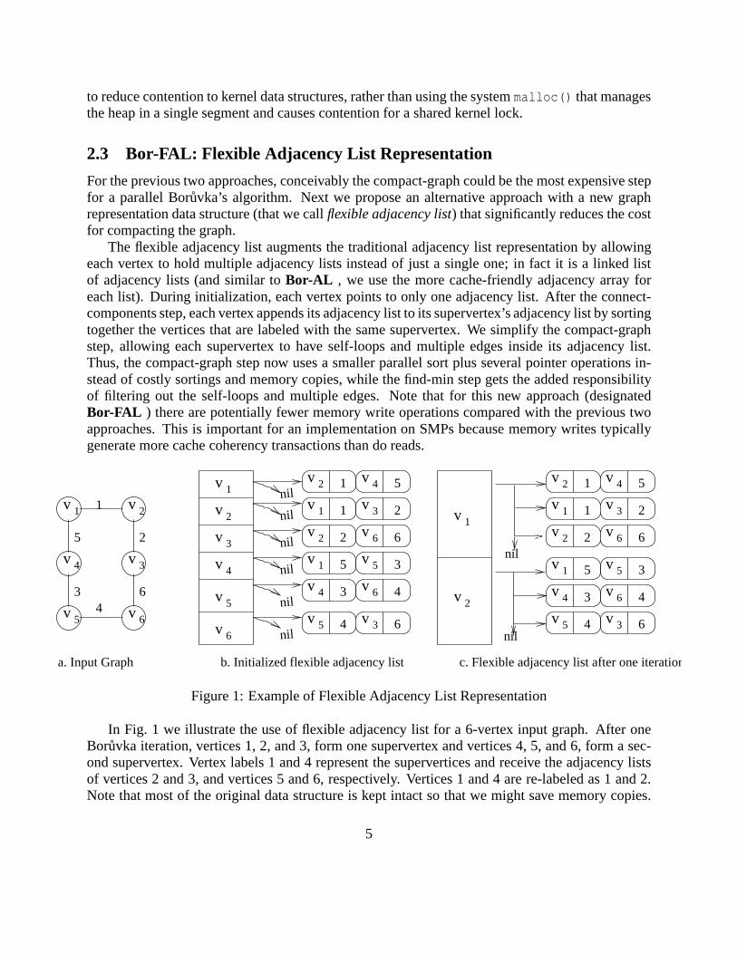
2.3 Bor-FAL: Flexible Adjacency List Representation

For the previous two approaches, conceivably the compact-graph could be the most expensive stepfor a parallel Bor˚uvka’s algorithm. Next we propose an alternative approach with a new graphrepresentation data structure (that we callflexible adjacency list) that significantly reduces the costfor compacting the graph.

The flexible adjacency list augments the traditional adjacency list representation by allowingeach vertex to hold multiple adjacency lists instead of just a single one; in fact it is a linked listof adjacency lists (and similar toBor-AL , we use the more cache-friendly adjacency array foreach list). During initialization, each vertex points to only one adjacency list. After the connect-components step, each vertex appends its adjacency list to its supervertex’s adjacency list by sortingtogether the vertices that are labeled with the same supervertex. We simplify the compact-graphstep, allowing each supervertex to have self-loops and multiple edges inside its adjacency list.Thus, the compact-graph step now uses a smaller parallel sort plus several pointer operations in-stead of costly sortings and memory copies, while the find-min step gets the added responsibilityof filtering out the self-loops and multiple edges. Note that for this new approach (designatedBor-FAL ) there are potentially fewer memory write operations compared with the previous twoapproaches. This is important for an implementation on SMPs because memory writes typicallygenerate more cache coherency transactions than do reads.

nil

1 5

1 2

2 6

5 3

3 4

4 6

1 5

1 2

2 6

5 3

3 4

4 6

nil

b. Initialized flexible adjacency list c. Flexible adjacency list after one iteration

nil

nil

nil

1

34

5 2

6

a. Input Graph

nil

nil

nil

v 4

v 5 v 6

v 2 v 4

v 1

v 2 v 6

v 1

v 4

v 1

v 2

v 3

v 4

v 5

v 6

v 1

v 2

v 1

v 3

v 2

v

5

v 6

v 5 v 3

v

5 v 3

v 3

v 5

v 6

v 2 v 4

v 1

v 2 v 6

v 3

v 1

v 4

Figure 1: Example of Flexible Adjacency List Representation

In Fig. 1 we illustrate the use of flexible adjacency list for a 6-vertex input graph. After oneBoruvka iteration, vertices 1, 2, and 3, form one supervertex and vertices 4, 5, and 6, form a sec-ond supervertex. Vertex labels 1 and 4 represent the supervertices and receive the adjacency listsof vertices 2 and 3, and vertices 5 and 6, respectively. Vertices 1 and 4 are re-labeled as 1 and 2.Note that most of the original data structure is kept intact so that we might save memory copies.

5

Instead of re-labeling vertices in the adjacency list, we maintain a separate lookup table that holdsthe supervertex label for each vertex. We easily obtain this table from the connect-componentsstep. The find-min step uses this table to filter out self-loops and multiple edges.

3 Analysis

Here we analyze the complexities of the different Bor˚uvka variants. Helman and J´aJa’s SMPcomplexity model [14] provides a reasonable framework for the realistic analysis that favors cache-friendly algorithms by penalizing non-contiguous memory accesses. Under this model, there aretwo parts to an algorithm’s complexity,ME the memory access complexity andTC the computationcomplexity. TheME term is the number of non-contiguous memory accesses, theTC term is therunning time. TheME term recognizes the effect that memory accesses have over an algorithm’sperformance. Parameters of the model includes the problem sizen and the number of processorsp.

For a sparse graphG with n vertices andm edges, as the algorithm iterates, the number ofvertices decreases by at least half in each iteration, so there are in total logn iterations for all of theBoruvka variants.

First we consider the complexity ofBor-EL . The find-min and connect-component steps arestraightforward, their aggregate complexity in one iteration is (assuming balanced load amongprocessors) is characterized by:

T(n, p) = 〈ME ; TC〉=⟨

n+nlognp

; O(

m+nlognp

)⟩. (1)

The parallel sample sort that we use inBor-EL for compact-graph has the complexity of

T(n, p) = 〈ME ; TC〉=⟨(

4+2clog l

p

logz

)lp

; O(

lp logl

)⟩(2)

with high probability wherel is the length of the list andc andz are constants related to cachesize and sampling ratio [14]. Aggregating the cost of sorting and the cost of manipulating the datastructure, we summarize the cost for compact-graph by

T(n, p) = 〈ME ; TC〉=⟨(

4+2clog(2m/p)

logz

)2mp

; O(

2mp log2m

)⟩. (3)

The value ofm decreases with each successive iteration dependent on the topology and edgeweight assignment of the input graph. Because the number of vertices is reduced by at least halfeach iteration,m decreases by at leastn

2 edges each iteration. For the sake of simplifying the anal-ysis, though, we usem unchanged as the number of edges during each iteration; clearly an upperbound of the worst case. Hence, the complexity ofBor-EL is given as

T(n, p) = 〈ME ; TC〉=⟨(

8m+n+nlognp

+4mclog(2m/p)

plogz

)logn ; O

(mp logmlogn

)⟩. (4)

6

We base this assumption on the following observation. For random sparse graphsm decreasesslowly in the first several iterations ofBor-EL , and the graph becomes denser (asn decreases at afaster rate thanm) until a certain point,m decreases drastically. Table 1 illustrates howm changesfor two random sparse graphs.

G1 = 1,000,000 vertices, 600,006 edgesG2 = 10,000 vertices, 30,024 edges

iteration 2m decrease % dec. m/n 2m decrease % dec. m/n

1 12000012 N/A N/A 6.0 60048 N/A N/A 3.02 10498332 1501680 12.5% 21.0 44782 15266 25.4% 8.93 10052640 445692 4.2% 98.1 34378 10404 23.2% 33.54 8332722 1719918 17.2% 472.8 6376 28002 80.5% 35.05 1446156 6886566 82.6% 534.8 156 6220 97.6% 6.06 40968 1405188 97.2% 100.9 2 154 98.7% 0.57 756 40212 98.2% 13.58 12 744 98.4% 1.5

Table 1: Example of the rate of decrease of the numberm of edges for two random sparse graphs.The 2m column gives the size of the edge list, thedecreasecolumn shows how much the size ofthe edge list decreases in the current iteration, the% dec.column gives the percentage that the sizeof the edge list decreases in the current iteration, andm/n shows the density of the graph.

In Table 1 for graphG1, 8 iterations are needed for Bor˚uvka’s algorithm. Until the 4th itera-tion, m is still more than half of its initial value. Yet at the next iteration,m drastically reduces toabout 1/10 of its initial value. Similar behavior is also observed forG2. As for a quite substantialnumber of iterationsm decreases slowly, for simplicity it is reasonable to assume thatm remainsunchanged (an upper bound for the actualm).

Table 1 also suggests that instead of growing a spanning tree for a relatively denser graph, if wecan exclude heavy edges in the early stages of the algorithm and decreasem, we may have a moreefficient parallel implementation for many input graphs because we might be able to greatly reducethe size of the edge list. After all, for a graph withm/n≥ 2, more than half of the edges are not inthe MST. In fact several MST algorithms exclude edges from the graph using the “cycle” property.Coleet al. [8] present a linear-work algorithm that first uses random sampling to find a spanningforestF of graphG, then identifies the heavy edges toF and excludes them from the final MST.The algorithm presented in [17], an inherently sequential procedure, also excludes edges accordingto the “cycle” property of MST.

Without going into the input-dependent details of how vertex degrees change as the Bor˚uvkavariants progress, we compare the complexity of the first iteration ofBor-AL with Bor-EL be-cause in each iteration these approaches compute similar results in different ways. ForBor-AL thecomplexity of the first iteration is

T(n, p) = 〈ME ; TC〉=⟨(

8n+5m+nlognp

+2nclog(n/p)+2mclog(m/n)

plogz

); O(

np logm+ m

p log(m/n))⟩

.

(5)

7

While for Bor-EL , the complexity of the first iteration is

T(n, p) = 〈ME ; TC〉=⟨(

8m+n+nlognp

+4mclog(2m/p)

plogz

); O(

mp logm

)⟩. (6)

We see thatBor-AL is a faster algorithm thanBor-EL , as expected, since the input forBor-AL is “bucketed” into adjacency lists, versusBor-EL that is an unordered list of edges, and sortingeach bucket first inBor-AL saves unnecessary comparisons between edges that have no verticesin common. We can consider the complexity ofBor-EL then to be an upper bound ofBor-AL .

In Bor-FAL n reduces at least by half whilem stays the same. Compact-graph first sorts thenvertices, then assigns O(n) pointers to append each vertex’s adjacency list to its supervertex’s. For

each processor, sorting takes O(

np logn

)time, and assigning pointers takes O(n/p) time assuming

each processor gets to assign roughly the same amount of pointers. Updating the lookup tablecosts each processor O(n/p) time. Asn decreases at least by half, the aggregate running time forcompact-graph is:

TC(n, p)cg =1p

logn

∑i=0

n2i log

n2i +

2p

logn

∑i=0

n2i = O

(nlogn

p

),ME(n, p)cg≤ 8n

p+

4cnlog(n/p)plogz

. (7)

With Bor-FAL , to find the smallest weight edge for the supervertices, all them edges willbe checked, each processor covering O(m/p) edges. The aggregate running time isTC(n, p) f m =O(mlogn/p) and the memory access complexity isME(n, p) f m = m/p. For the finding connected

component step, each processor takesTcc = O(

nlog np

)time, andME(n, p)cc≤ 2nlogn.

The complexity for the whole Bor˚uvka’s algorithm is:

T(n, p) = T(n, p) f m+T(n, p)cc+T(n, p)cg (8)

≤⟨

8n+2nlogn+mlognp

+4cnlog(n/p)

plogz; O(

m+np logn

)⟩

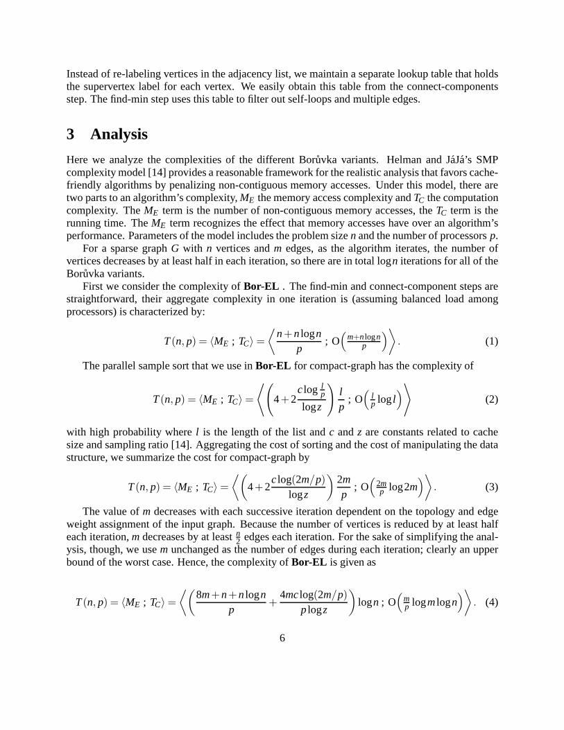
It would be interesting and important to check how well our analysis and claim fit with theactual experiments. Detailed performance results are presented in Section 5, here we show thatBor-AL in practice runs faster thanBor-EL and Bor-FAL greatly reduces the compact-graphtime. Fig. 2 shows for the three approaches the breakdown of the running time for the three steps.

Immediately we can see that forBor-EL andBor-AL the compact-graph step dominates therunning time.Bor-EL takes much more time thanBor-AL , and only gets worse when the graphsget denser. In contrast the execution time of compact-graph step ofBor-FAL is greatly reduced,in the experimental section with a random graph of 1M vertices and 10M edges, it is over 50 timesfaster thanBor-EL , and over 7 times faster thanBor-AL . Actually the execution time of thecompact-graph step ofBor-FAL is almost the same for the three input graphs because it only de-pends on the number of vertices. As predicted, the execution time of the find-min step ofBor-FALincreases. And the connect-components step only takes a small fraction of the execution time forall approaches.

8

Figure 2: Breakdown of the running time for the three steps of the three approaches. Stack barsare organized into three groups by the input graphs that are random graphs with fixed 1M verticesand 4M, 6M and 10M edges respectively. Inside each group, the bars from left-to-right representBor-EL , Bor-AL , Bor-ALM , andBor-FAL , respectively.

9

4 A New Parallel MST Algorithm For Shared-Memory

In this section we present a new non-deterministic shared-memory algorithm for finding a mini-mum spanning tree/forest that is quite different from Bor˚uvka’s approach in that it uses multiple,coordinated instances of Prim’s sequential algorithm running on the graph’s shared data structure.In fact, the new approach marries Prim’s algorithm (known as an efficient sequential algorithm forMST) with that of the naturally parallel Bor˚uvka approach. In our new algorithm essentially we leteach processor simultaneously run Prim’s algorithm from different starting vertices. We say a treeis growingwhen there exists a lightweight edge that connects the tree to a vertex not yet in anothertree, andmatureotherwise. When all of the vertices have been incorporated into mature subtrees,we contract each subtree into a supervertex and call the approach recursively until only one super-vertex remains. When the problem size is small enough, one processor solves the remaining prob-lem using the best sequential MST algorithm. If no edges remain between supervertices, we haltthe algorithm and return the minimum spanning forest. The detailed algorithm is given in Alg. 1.

In Alg. 1, step 1 initializes each vertex as uncolored and unvisited. A processorcolorsa vertexif it is the first processor to insert it into a heap, and labels a vertex asvisitedwhen it is extractedfrom the heap; i.e., the edge associated with the vertex has been selected to be in the MST. In step 2(Alg. 2) each processor first searches its own portion of the list for uncolored vertices from whichto start Prim’s algorithm. In each iteration a processor chooses a unique color (different from otherprocessors’ colors or the colors it has used before) as its own color. After extracting the minimumelement from the heap, the processor checks whether the element is colored by itself, and if not, acollision with another processor occurs (meaning multiple processors try to color this element ina race) , the processor stops growing the current sub-MST. Otherwise it continues. In Appendix Bwe prove that Alg. 1 finds an MST of the graph.

The algorithm as given may not keep all of the processors equally busy, since each may visita different number of vertices during an iteration. We balance the load simply by using the workstealing technique as follows. When a processor completes its partition ofn

p vertices, an unfinishedpartition is randomly selected, and processing begins from a decreasing pointer that marks the endof the unprocessed list. It is theoretically possible that no edges are selected for the growing trees,and hence, no progress made during an iteration of the algorithm (although this case is highly un-likely in practice). For example, if the input containedn

p cycles, with cyclei defined as vertices{i n

p,(i+1) np, . . . ,(i+ p−1) n

p}, for 0≤ i < np, and if the processors are perfectly synchronized, each

vertex would be a singleton in its own mature tree. A practical solution that guarantees progresswith high probability is to randomly reorder the vertex set, which can be done simply in paralleland without added asymptotic complexity [30].

4.1 Analysis

Our new parallel MST algorithm possesses an interesting feature: when run on one processor thealgorithm behaves as Prim’s, and onn processors becomes Bor˚uvka’s, and runs as a hybrid combi-nation for 1< p < n, wherep is the number of processors. In addition, our new algorithm is novelwhen compared with Bor˚uvka’s approach in the following ways.

10

Input : GraphG = (V,E) represented by adjacency listA with n = |V|nb: the base problem size to be solved sequentially.

Output : MSF for graphGbegin

while n > nb and m> n−1 do1. Initialized thecolor andvisitedarraysfor v← i n

p to (i +1) np−1 do

color[v] = 0,visited[v] = 02. Run Alg. 2.3. for v← i n

p to (i +1) np−1 do

if visited[v] = 0 then find the lightest incident edgee to v, and labele to be inMST

4. With the found MST edges, run connected components on the induced graph,and shrink each component into a supervertex5. Setn← the number of supervertices; andm← the number of edges between thesupervertices

6. if m> n−1 then solve the problem on one processorelseselect remainingm edgesend

Algorithm 1: Parallel algorithm for new MSF approach, for processorpi , for (0≤ i ≤ p−1).Assume w.l.o.g. thatp dividesn evenly.

11

Input : (1) p processors, each with processor IDpi , (2) a partition of adjacency list for eachprocessor (3) arraycolor andvisited

Output : A spanning forest that is part of graphG’s MSTbegin

1. for v← i np to (i +1) n

p−1 do1.1 if color[v] 6= 0 then v is already colored, continue1.2n = n+1, my color = np+ pi , color[v] = my color1.3 insertv into heapH1.4while H is not emptydo

w = heapextractmin(H)if (color[w] 6= my color) OR (any neighbor u of w hascolor other than0 ormy color) then breakif visited[w] = 0 then

visited[w] = 1, and label the corresponding edgeeas in MSTfor each neighbor u of wdo

if color[u] = 0 then color[u] = my colorif u in heap Hthen heapdecreasekey(u,h)elseheapinsert(u,H)

end

Algorithm 2: Parallel algorithm for new MST approach based on Prim’s that finds parts ofMST, for processorpi , for (0≤ i ≤ p−1). Assume w.l.o.g. thatp dividesn evenly.

12

1. Each ofp processors in our algorithm finds for its starting vertex the smallest-weight edge,contracts that edge, and then finds the smallest-weight edge again for the contracted super-vertex. We do not find all the smallest-weight edges for all vertices, synchronize, and thencompact as in the parallel Bor˚uvka’s algorithm.

2. Our algorithm adapts for any numberp of processors in a practical way for SMPs, wherep is often much less thann, rather than in parallel implementations of Bor˚uvka’s approachthat appear as PRAM emulations withp coarse-grained processors that emulaten virtualprocessors.

The performance of our new algorithm is dependent on its granularitynp, for 1≤ p≤ n. The

worst-case is when the granularity is small, i.e., a granularity of 1 whenp = n and the approachturns to Boruvka . Hence, the worst case complexities are similar to that of the parallel Bor˚uvkavariants analyzed previously. Yet in practice we expect our algorithm to perform better than parallelBoruvka’s algorithm on sparse graphs because their lower connectivity implies that our algorithmbehaves likep simultaneous copies of Prim’s algorithm with some synchronization overhead.

5 Experimental Results

This section summarizes the experimental results of our implementations and compares our re-sults with previous experimental results. We tested our shared-memory implementation on the SunE4500, a uniform-memory-access (UMA) shared memory parallel machine with 14 UltraSPARCII 400MHz processors and 14 GB of memory. Each processor has 16 Kbytes of direct-mapped data(L1) cache and 4 Mbytes of external (L2) cache. The algorithms are implemented using POSIXthreads and a library of parallel primitives developed by our group [3].

5.1 Experimental Data

Next we describe the collection of sparse graph generators that we use to compare the perfor-mance of the parallel minimum spanning tree graph algorithms. Our generators include severalemployed in previous experimental studies of parallel graph algorithms for related problems. Forinstance, we include the2D60and3D40mesh topologies used in the connected component studiesof [13, 21, 15, 12], the random graphs used by [13, 7, 15, 12], and the geometric graphs used by[13, 15, 21, 12, 7].

• Regular and Irregular MeshesComputational science applications for physics-based sim-ulations and computer vision commonly use mesh-based graphs. All of the edge weights areuniformly random.

– 2D MeshThe vertices of the graph are placed on a 2D mesh, with each vertex con-nected to its four neighbors whenever they exist.

– 2D602D mesh with the probability of 60% for each edge to be present.– 3D403D mesh with the probability of 40% for each edge to be present.

13

• Structured Graphs These graphs are used by Chung and Condon (see [7] for detailed de-scriptions) to study the performance of parallel Bor˚uvka’s algorithm. They have recursivestructures that correspond to the iteration of Bor˚uvka’s algorithm and are degenerate (theinput is already a tree).

– str0 At each iteration withn vertices, two vertices form a pair. So with Bor˚uvka’salgorithm, the number of vertices decrease exactly by a half in each iteration. In termof the number of iterations,str0 is a worst case for parallel Bor˚uvka’s algorithm.

– str1 At each iteration withn vertices,√

n vertices form a linear chain.– str2 At each iteration withn vertices,n/2 vertices form linear chain, and the othern/2

form pairs.– str3 At each iteration withn vertices,

√n vertices form a complete binary tree.

• Random Graph We create a random graph ofn vertices andmedges by randomly addingmunique edges to the vertex set. Several software packages generate random graphs this way,including LEDA [24]. The edge weights are selected uniformly and at random.

• Geometric GraphsIn these graphs, we give each vertex a fixed degreek. Moret and Shapiro[25] use these in their empirical study of sequential MST algorithms.

5.2 Performance Results and Analysis

In this section we offer a collection of our performance results that demonstrate for the first timea parallel minimum spanning tree implementation that exhibits speedup when compared with thebest sequential approach over a wide range of sparse input graphs. We implemented three sequen-tial algorithms: Prim’s algorithm with binary heap, Kruskal’s algorithm with non-recursive mergesort (which in our experiments has superior performance over qsort, GNU quicksort, and recursivemerge sort for large inputs) and themlogm Boruvka’s algorithm.

Previous studies such as [7] compare their parallel implementations with sequential Bor˚uvka(even though they reported that sequential Bor˚uvka was several times slower than other MST algo-rithms) and Kruskal’s algorithm. We observe Prim’s algorithm can be 3 times faster than Kruskal’salgorithm for some inputs. Density of the graphs is not the only determining factor of the perfor-mance ranking of the three sequential algorithms. Different assignment of edge weights is alsoimportant. Fig. 3 shows the performance rankings of the three sequential algorithms over a rangeof our input graphs.

In our performance results we specify which sequential algorithm achieves the best result forthe input and use this algorithm when determining parallel speedup. In our experimental stud-ies,Bor-EL , Bor-AL , Bor-ALM , andBor-FAL , are the parallel Bor˚uvka variants using edgelists, adjacency lists, adjacency lists and our memory management, and flexible adjacency lists,respectively.MST-BC is our new minimum spanning forest parallel algorithm.

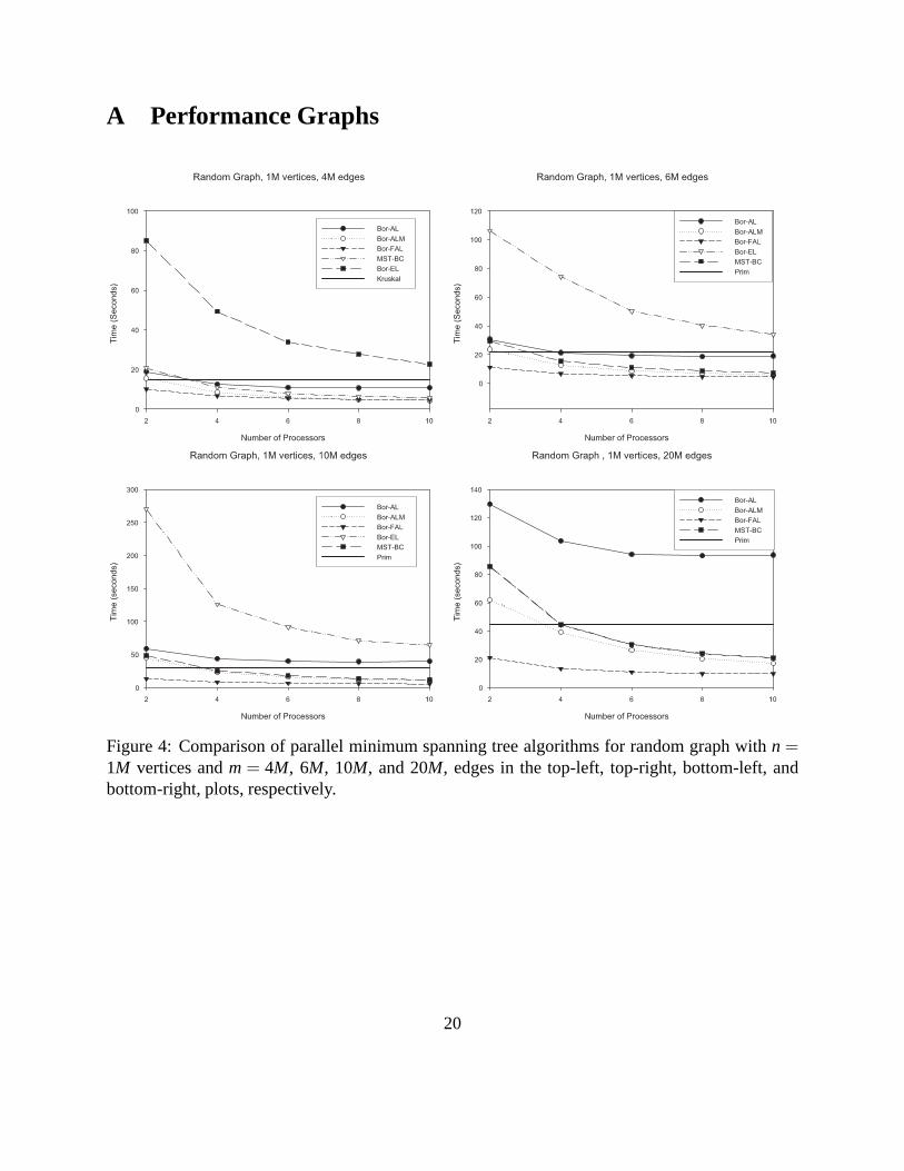
In Appendix A we present a summary of our performance results. The performance plots inFig. 4 are for the random graphs, in Fig. 5 are for the regular and irregular meshes (mesh,2D60, and3D40) and a geometric graph withk = 6, and in Fig. 6 are for the structured graphs. In these plots,

14

Figure 3: Different performance rankings for the three sequential algorithms over different inputgraph types.

15

the thick horizontal line represents the time taken for the best sequential MST algorithm (named ineach legend) to find a solution on the same input graph using a single processor on the Sun E4500.

For the random, sparse graphs, we find that our Bor˚uvka variant with flexible adjacency listsoften has superior performance, with a speedup of approximately 5 using 8 processors over thebest sequential algorithm (Prim’s in this case). In the regular and irregular meshes, the adjacencylist representation with our memory management (Bor-ALM ) often is the best performing parallelapproach with parallel speedups near 6 for 8 processors. Finally, for the structured graphs thatare worst-cases for Bor˚uvka algorithms, our new MST algorithm often is the only approach thatruns faster than the sequential algorithm, although speedups are more modest with at most 4 for 8processors in some instances.

6 Conclusions and Future Work

In summary, we present optimistic results that for the first time, show that parallel minimum span-ning tree algorithms run efficiently on parallel symmetric multiprocessors for graphs with irregulartopologies. We present a new nondeterministic MST algorithm that uses a load balancing schemebased upon work stealing that, unlike Bor˚uvka variants, gives some speedup compared with thebest sequential algorithms on several structured inputs that are hard to achieve parallel speedup.Through comparison with the best sequential implementation, we see our implementations ex-hibiting parallel speedup, which is remarkable to note since the sequential algorithm has very lowoverhead. Further, these results provide optimistic evidence that complex graph problems thathave efficient PRAM solutions, but often no known efficient parallel implementations, may scalegracefully on SMPs. Our future work includes validating these experiments on larger SMPs, andsince the code is portable, on other vendors’ platforms. We plan to apply the techniques discussedin this paper to other related graph problems, for instance, maximum flow, connected components,and planarity testing algorithms, for symmetric multiprocessors.

16

References

[1] M. Adler, W. Dittrich, B. Juurlink, M. Kutylowski, and I. Rieping. Communication-optimalparallel minimum spanning tree algorithms. InProc. 10th Ann. Symp. Parallel Algorithmsand Architectures (SPAA-98), pages 27–36, Newport, RI, June 1998. ACM.

[2] L. An, Q.S. Xiang, and S. Chavez. A fast implementation of the minimum spanning treemethod for phase unwrapping.IEEE Trans. Med. Imaging, 19(8):805–808, 2000.

[3] D. A. Bader and J. J´aJa. SIMPLE: A methodology for programming high performance algo-rithms on clusters of symmetric multiprocessors (SMPs).J. Parallel & Distributed Comput.,58(1):92–108, 1999.

[4] M. Brinkhuis, G.A. Meijer, P.J. van Diest, L.T. Schuurmans, and J.P. Baak. Minimum span-ning tree analysis in advanced ovarian carcinoma.Anal. Quant. Cytol. Histol., 19(3):194–201,1997.

[5] C. Chen and S. Morris. Visualizing evolving networks: Minimum spanning trees versuspathfinder networks. InIEEE Symp. on Information Visualization, Seattle, WA, October2003. to appear.

[6] K. W. Chong, Y. Han, and T. W. Lam. Concurrent threads and optimal parallel minimumspanning tree algorithm.J. ACM, 48:297–323, 2001.

[7] S. Chung and A. Condon. Parallel implementation of Bor˚uvka’s minimum spanning treealgorithm. InProc. 10th Int’l Parallel Processing Symp. (IPPS’96), pages 302–315, April1996.

[8] R. Cole, P.N. Klein, and R. E. Tarjan. Finding minimum spanning forests in logarithmic timeand linear work using random sampling. InProc. 8th Ann. Symp. Parallel Algorithms andArchitectures (SPAA-96), pages 243–250, Newport, RI, June 1996. ACM.

[9] R. Cole, P.N. Klein, and R.E. Tarjan. A linear-work parallel algorithm for finding minimumspanning trees. InProc. 6th Ann. Symp. Parallel Algorithms and Architectures (SPAA-94),pages 11–15, Newport, RI, June 1994. ACM.

[10] F. Dehne and S. G¨otz. Practical parallel algorithms for minimum spanning trees. InWork-shop on Advances in Parallel and Distributed Systems, pages 366–371, West Lafayette, IN,October 1998. co-located with the 17th IEEE Symp. on Reliable Distributed Systems.

[11] J.C. Dore, J. Gilbert, E. Bignon, A. Crastes de Paulet, T. Ojasoo, M. Pons, J.P. Raynaud, andJ.F. Miquel. Multivariate analysis by the minimum spanning tree method of the structuraldeterminants of diphenylethylenes and triphenylacrylonitriles implicated in estrogen receptorbinding, protein kinase C activity, and MCF7 cell proliferation.J. Med. Chem., 35(3):573–583, 1992.

17

[12] S. Goddard, S. Kumar, and J.F. Prins. Connected components algorithms for mesh-connectedparallel computers. In S. N. Bhatt, editor,Parallel Algorithms: 3rd DIMACS ImplementationChallenge October 17-19, 1994, volume 30 ofDIMACS Series in Discrete Mathematics andTheoretical Computer Science, pages 43–58. American Mathematical Society, 1997.

[13] J. Greiner. A comparison of data-parallel algorithms for connected components. InProc. 6thAnn. Symp. Parallel Algorithms and Architectures (SPAA-94), pages 16–25, Cape May, NJ,June 1994.

[14] D. R. Helman and J. J´aJa. Designing practical efficient algorithms for symmetric multiproces-sors. InAlgorithm Engineering and Experimentation (ALENEX’99), volume 1619 ofLectureNotes in Computer Science, pages 37–56, Baltimore, MD, January 1999. Springer-Verlag.

[15] T.-S. Hsu, V. Ramachandran, and N. Dean. Parallel implementation of algorithms for findingconnected components in graphs. In S. N. Bhatt, editor,Parallel Algorithms: 3rd DIMACSImplementation Challenge October 17-19, 1994, volume 30 ofDIMACS Series in DiscreteMathematics and Theoretical Computer Science, pages 23–41. American Mathematical So-ciety, 1997.

[16] J. JaJa. An Introduction to Parallel Algorithms. Addison-Wesley Publishing Company, NewYork, 1992.

[17] I. Katriel, P. Sanders, and J. L. Tr¨aff. A practical minimum spanning tree algorithm usingthe cycle property. Technical Report MPI-I-2002-1-003, MPI Informatik, Germany, October2002.

[18] I. Katriel, P. Sanders, and J. L. Tr¨aff. A practical minimum spanning tree algorithm usingthe cycle property. In11th Ann. European Symp. on Algorithms (ESA 2003), Budapest,September 2003. to appear.

[19] K. Kayser, S.D. Jacinto, G. Bohm, P. Frits, W.P. Kunze, A. Nehrlich, and H.J. Gabius. Appli-cation of computer-assisted morphometry to the analysis of prenatal development of humanlung. Anat. Histol. Embryol., 26(2):135–139, 1997.

[20] K. Kayser, H. Stute, and M. Tacke. Minimum spanning tree, integrated optical density andlymph node metastasis in bronchial carcinoma.Anal. Cell Pathol., 5(4):225–234, 1993.

[21] A. Krishnamurthy, S. S. Lumetta, D. E. Culler, and K. Yelick. Connected components ondistributed memory machines. In S. N. Bhatt, editor,Parallel Algorithms: 3rd DIMACSImplementation Challenge October 17-19, 1994, volume 30 ofDIMACS Series in DiscreteMathematics and Theoretical Computer Science, pages 1–21. American Mathematical Soci-ety, 1997.

18

[22] M. Matos, B.N. Raby, J.M. Zahm, M. Polette, P. Birembaut, and N. Bonnet. Cell migrationand proliferation are not discriminatory factors in the in vitro sociologic behavior of bronchialepithelial cell lines.Cell Motility and the Cytoskeleton, 53(1):53–65, 2002.

[23] S. Meguerdichian, F. Koushanfar, M. Potkonjak, and M. Srivastava. Coverage problems inwireless ad-hoc sensor networks. InProc. INFOCOM ’01, pages 1380–1387, Anchorage,AK, April 2001. IEEE Press.

[24] K. Mehlhorn and S. N¨aher.The LEDA Platform of Combinatorial and Geometric Computing.Cambridge University Press, 1999.

[25] B.M.E. Moret and H.D. Shapiro. An empirical assessment of algorithms for constructinga minimal spanning tree. InDIMACS Monographs in Discrete Mathematics and Theoreti-cal Computer Science: Computational Support for Discrete Mathematics15, pages 99–117.American Mathematical Society, 1994.

[26] V. Olman, D. Xu, and Y. Xu. Identification of regulatory binding sites using minimum span-ning trees. InProc. 8th Pacific Symp. Biocomputing (PSB 2003), pages 327–338, Hawaii,2003. World Scientific Pub.

[27] J. Park, M. Penner, and V.K. Prasanna. Optimizing graph algorithms for improved cacheperformance. InProc. Int’l Parallel and Distributed Processing Symp. (IPDPS 2002), FortLauderdale, FL, April 2002.

[28] S. Pettie and V. Ramachandran. A randomized time-work optimal parallel algorithm forfinding a minimum spanning forest.SIAM J. Comput., 31(6):1879–1895, 2002.

[29] C.K. Poon and V. Ramachandran. A randomized linear work EREW PRAM algorithm tofind a minimum spanning forest. InProc. 8th Int’l Symp. Algorithms and Computation(ISAAC’97), volume 1350 ofLecture Notes in Computer Science, pages 212–222. Springer-Verlag, 1997.

[30] P. Sanders. Random permutations on distributed, external and hierarchical memory.Infor-mation Processing Letters, 67(6):305–309, 1998.

[31] Y.-C. Tseng, T.T.-Y. Juang, and M.-C. Du. Building a multicasting tree in a high-speednetwork. IEEE Concurrency, 6(4):57–67, 1998.

[32] S.Q. Zheng, J.S. Lim, and S.S. Iyengar. Routing using implicit connection graphs. In9thInt’l Conf. on VLSI Design: VLSI in Mobile Communication, Bangalore, India, January 1996.IEEE Computer Society Press.

19

A Performance Graphs

Figure 4: Comparison of parallel minimum spanning tree algorithms for random graph withn =1M vertices andm = 4M, 6M, 10M, and 20M, edges in the top-left, top-right, bottom-left, andbottom-right, plots, respectively.

20

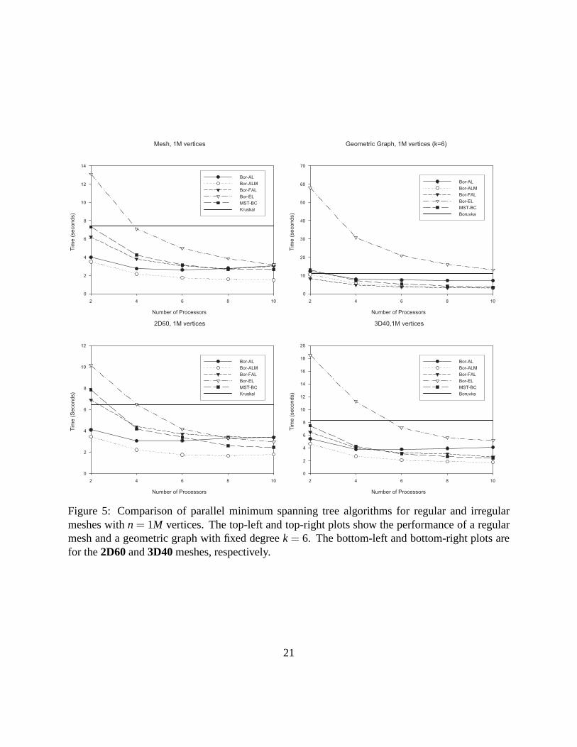
Figure 5: Comparison of parallel minimum spanning tree algorithms for regular and irregularmeshes withn = 1M vertices. The top-left and top-right plots show the performance of a regularmesh and a geometric graph with fixed degreek = 6. The bottom-left and bottom-right plots arefor the2D60and3D40meshes, respectively.

21

Figure 6: Comparison of parallel minimum spanning tree algorithms for the structured graphsstr0,str1, str2, andstr3, in the top-left, top-right, bottom-left, and bottom-right, plots, respectively.

22

B Proofs

We prove that Alg. 1 finds a MST of the graph. Note that we assume without loss of generalitythat all the edges have distinct weights.

Lemma 1 On an SMP with sequential memory consistency, subtrees grown by Alg. 2 do not toucheach other, in other words, no two subtrees share a vertex.

Proof: Step 1.4 of Alg. 2 grows subtrees following the fashion of Prim’s algorithm. Supposetwo subtreesT1 andT2 share one vertexv. We have two cases:

• case 1:T1 andT2 could be two trees grown by one processor, or

• case 2: each tree is grown by a different processor.

v will be included in a processor’s subtree only if when it is extracted from the heap and foundto be colored as the processor’s current color (Step 1.4 of Alg. 2).

(case 1) IfT1 andT2 are grown by the same processorpi (also assume without loss of generalityT1 is grown beforeT2 in iterationsk1 andk2 respectively withk1 < k2), and processorpi choosesa unique color to color the vertices (Step 1.2 of Alg. 2), thenv is coloredk1p+ i in T1, and latercolored again inT2 with a different colork2p+ i. As before coloring a vertex, each processorwill first checks whether it has already been colored (Step 1.1 of Alg. 2), this means when pro-cessorpi checks whetherv has been colored, it does not see the previous coloring. This is a clearcontradiction of sequential memory consistency.

(case 2) Assume thatv is a vertex found in two treesT1 andT2 grown by two processorsp1 andp2, respectively. We denotetv as the time thatv is colored. Suppose whenv is added toT1, it isconnected to vertexv1, and when it is added toT2, it is connected tov2. Sincev is connected tov1

andv2, we have thattv1 < tv andtv2 < tv. Also tv < tv1 andtv < tv2 since after addingv to T1 we havenot seen the coloring ofv2 yet, and similarly after addingv to T2 we have not seen the coloringof v1 yet. This is a contradiction of step 1.4 in Alg. 2, and hence, a vertex will not be included inmore than one growing tree.

2

Lemma 2 No cycles are formed by the edges found in Alg. 1.

Proof: In Step 2 of Alg. 1, each processor grows sub-trees. Following lemma. 1, no cycles areformed among these trees. Step 5 of Alg. 1 is the only other step that labels edges, and the edgesfound in this step do not form cycles among themselves (otherwise it is a direct contradiction of thecorrectness of Bor˚uvka’s algorithm). Also these edges do not form any cycles with the sub-treesgrown in step 2. To see this, note that each of these edges has at least one endpoint that is notshared by any of the sub-trees, so the sub-trees can be treated as “vertices.” Supposel such edgesandm subtrees form a cycle, we havel edges andl + m vertices, which meansm= 0. Similarly

23

edges found in step 5 do not connect two subtrees together, but may increase the sizes of subtrees.2

Lemma 3 Edges found in Alg. 1 are in the MST.

Proof: Consider a single iteration of Alg. 1 on graphG. Assume after step 5, we run parallelBoruvka’s algorithm to get the minimum spanning tree for the reduced graph. Now we prove thatfor the spanning treeT we get fromG, every edgee of G that is not inT is aT-heavy edge. Letsconsider the following cases:

• Two endpoints ofe are in two different subtrees. Obviouslye is T-heavy because we runBoruvka’s algorithm to get the minimum spanning tree of the reduced graph (in which eachsubtree is now a vertex) .

• Two endpointsu, v of e are in the same sub-tree that is generated by step 1.4. According toPrim’s algorithme is T-heavy.

• Two endpointsu,v of eare in the same sub-tree,u is in the part grown by step 1.4 andv is inpart grown by step 3. It is easy to prove thate has larger weight than all the weights of theedges along the path fromu to v in T.

• Two endpointsu, v are in the the same subtree, bothu andv are in parts generated by step 5.Againe is T-heavy.

In summary, we have a spanning treeT, yet all the edges ofG that are not inT areT-heavy, soTis a MST.2

Theorem 1 For connected graph G, Alg. 1 finds the MST of G.

Proof:Theorem 1 follows by repeatedly applying Lemma 3.2

24