Approximation Algorithms for Minimum-Loadk-Facility Location

Sara Ahmadian∗1, Babak Behsaz2, Zachary Friggstad2, Amin Jorati2,Mohammad R. Salavatipour†2, and Chaitanya Swamy‡1

1 Department of Combinatorics and Optimization, University of WaterlooWaterloo, ON, Canada, N2L 3G1sahamdian,cswamy@math.uwaterloo.ca

2 Department of Computing Science, University of AlbertaEdmonton, AB, Canada, T6G 2E8behsaz,zacharyf,jorati,mrs@ualberta.ca

AbstractWe consider a facility-location problem that abstracts settings where the cost of serving the clients as-signed to a facility is incurred by the facility. Formally, we consider the minimum-load k-facility location(MLkFL) problem, which is defined as follows. We have a set F of facilities, a set C of clients, andan integer k ≥ 0. Assigning client j to a facility f incurs a connection cost d(f, j). The goal is toopen a set F ⊆ F of k facilities, and assign each client j to a facility f(j) ∈ F so as to minimizemaxf∈F

∑j∈C:f(j)=f d(f, j); we call

∑j∈C:f(j)=f d(f, j) the load of facility f . This problem was

studied under the name of min-max star cover in [6, 2], who (among other results) gave bicriteria ap-proximation algorithms for MLkFL for when F = C. MLkFL is rather poorly understood, and only anO(k)-approximation is currently known for MLkFL, even for line metrics.

Our main result is the first polynomial time approximation scheme (PTAS) for MLkFL on line metrics(note that no non-trivial true approximation of any kind was known for this metric). Complementing this,we prove that MLkFL is strongly NP-hard on line metrics. We also devise a quasi-PTAS for MLkFLon tree metrics. MLkFL turns out to be surprisingly challenging even on line metrics, and resilient toattack by the variety of techniques that have been successfully applied to facility-location problems. Forinstance, we show that: (a) even a configuration-style LP-relaxation has a bad integrality gap; and (b) amulti-swap k-median style local-search heuristic has a bad locality gap. Thus, we need to devise variousnovel techniques to attack MLkFL.

Our PTAS for line metrics consists of two main ingredients. First, we prove that there always exists anear-optimal solution possessing some nice structural properties. A novel aspect of this proof is that wefirst move to a mixed-integer LP (MILP) encoding the problem, and argue that a MILP-solution minim-izing a certain potential function possesses the desired structure, and then use a rounding algorithm forthe generalized-assignment problem to “transfer” this structure to the rounded integer solution. Comple-menting this, we show that these structural properties enable one to find such a structured solution viadynamic programming.

1998 ACM Subject Classification F.2.2 Nonnumerical Algorithms and Problems

Keywords and phrases approximation algorithms, min-max star cover, facility location, line metrics

Digital Object Identifier 10.4230/LIPIcs.xxx.yyy.p

∗ Supported by the last author’s NSERC grant 327620-09.† Supported by NSERC.‡ Supported in part by NSERC grant 327620-09, an NSERC Discovery Accelerator Supplement Award, and an

Ontario Early Researcher Award.

© Sara Ahmadian, Babak Behsaz, Zachary Friggstad, Amin Jorati, Mohammad R. Salavatipour, and Chaitanya Swamy;licensed under Creative Commons License CC-BY

Conference title on which this volume is based on.Editors: Billy Editor and Bill Editors; pp. 1–16

Leibniz International Proceedings in InformaticsSchloss Dagstuhl – Leibniz-Zentrum für Informatik, Dagstuhl Publishing, Germany

2 Approximation Algorithms for Minimum-Load k-Facility Location

1 Introduction

Facility-location (FL) problems have been widely studied in the Operations Research and ComputerScience communities (see, e.g., [13] and the survey [16]), and have a wide range of applications.These problems are typically described in terms of an underlying set of clients that require service,and a candidate set of facilities that provide service to these clients. The goal is to determine whichfacilities to open, and decide how to assign clients to open facilities to minimize some combinationof the facility-opening and client-connection (a.k.a service) costs. An oft-cited prototypical exampleis that of a company wanting to decide where to locate its warehouses/distribution centers so as toserve its customers in a cost-effective manner.

We consider settings where the cost of serving the clients assigned to a facility is incurred bythe facility; for instance, in the above example, each warehouse may be responsible for supplyingits clients and hence bears a cost equal to the total cost of servicing its clients. In such settings, it isnatural to consider the problem of minimizing the maximum cost borne by any facility. Formalizingthis, we consider the following mathematical model. We are given a set F of facilities, a set C ofclients, and an integer k ≥ 0. Assigning client j to a facility f incurs a connection or service costd(f, j). There are no facility-opening costs. The goal is to open k facilities from F and assign eachclient j to an open facility f(j) so as to minimize the maximum load of an open facility, wherethe load of an open facility f is defined as

∑j∈C:f(j)=f d(f, j); that is, the load of f is the total

connection cost incurred for the clients assigned to it. We call this the minimum-load k-facilitylocation (MLkFL) problem. As is common in the study of facility-location problems, we assumethat the clients and facilities lie in a common metric space, so the d(f, j)s form a metric.

Despite the extensive amount of literature on facility-location problems, there is surprisinglylittle amount of work on MLkFL and it remains a rather poorly understood problem (see [15]). Onecan infer that the problem is NP-hard, even when the set of open facilities is fixed, via a reductionfrom the makespan-minimization problem on parallel machines, and that an O(k)-approximationcan be obtained by running any of the various O(1)-approximation algorithms for k-median [4, 9,8, 3, 12] (where one seeks to minimize the sum of the facility loads). No better approximationalgorithms are known for MLkFL even on line metrics, and this was mentioned as an open problemin [15]. The only work on approximation algorithms for this problem that we are aware of is due toEven et al. [6] and Arkin et al. [2], who refer to this problem as min-max star cover (where F = C).1

Both works obtain bicriteria approximation algorithms for MLkFL in general metrics, which meansthat the algorithm returns a solution with near-optimal maximum load but may need to open morethan k facilities. For MLkFL on star metrics and whenF = C, someO(1)-approximation algorithmsfollow from work on minimum-makespan scheduling and [6, 2] (see “Related work”).

1.1 Our results.

We completely resolve the status of min-load k-FL on line metrics. As we elaborate below (see“Our techniques”), MLkFL turns out to be surprisingly challenging even on line metrics, and seemsresilient to attack by the variety of techniques that have been successfully applied to facility-locationproblems, including LP-rounding, local search, and primal-dual methods. Our main result is that des-pite these difficulties, one can devise a polynomial-time approximation scheme (PTAS) for MLkFLon line metrics (Theorem 1). As mentioned earlier, this is the first approximation algorithm forMLkFL on line metrics that achieves anything better than an O(k)-approximation.

We also consider MLkFL in tree metrics (Section 4). First, we observe that the quasi-PTAS

1 Jorati [10], in his Master’s thesis, obtained a preliminary version of some of our current results.

S. Ahmadian, B. Behsaz, Z. Friggstad, A. Jorati, M. R. Salavatipour, and C. Swamy 3

obtained by Jorati [10] for line metrics extends to yield a quasi-PTAS (QPTAS) for tree metrics(Theorem 9). Next, we consider the special case of star metrics, but in the more-general settingwhere clients may have non-uniform integer demands Djj∈C and the demand of a client maybe split integrally between several open facilities. We now define the load of a facility f to be∑j xfjd(f, j), where xfj ∈ Z≥0 is the amount of j’s demand that is assigned to f . We devise a

14-approximation algorithm for MLkFL on star metrics with non-uniform demands (Theorem 10).Notice that when we restrict the metric to be a star metric, we cannot create colocated copies of aclient (without destroying the star topology), which makes the setting with non-uniform demandsstrictly more general than the unit-demand setting.

In Section 5, we obtain various computational-complexity and integrality-gap lower bounds forMLkFL. Complementing our PTAS, we show (Theorem 11) that MLkFL is strongly NP-hard online metrics (and hence, a PTAS is the best approximation that one can hope to achieve in polytimeunless P =NP). We also show that MLkFL is APX-hard in the Euclidean plane (Theorem 12). Finally,we justify our comment about the difficulty of tackling MLkFL via the various LP-based methodsdeveloped for facility-location problems by showing that even a configuration-style LP-relaxation forMLkFL—where we “guess” the optimum value B and have a variable xf,S for every facility f andevery possible set S of clients such that

∑j∈S d(f, j) ≤ B—has an integrality gap of Ω(k/ log k)

even for line metrics (Theorem 13). Note that the configuration LP is stronger than the natural LP-relaxation for MLkFL. Moreover, this holds even if the graph consisting of the edges (j, f) suchthat d(j, f) ≤ B—call these feasible edges—is connected. This is in contrast with capacitated k-center [5, 1], where a large integrality gap for the natural LP arises due to the fact that the graph offeasible edges is disconnected.

1.2 Our techniques.

Before detailing the techniques underlying our PTAS for line metrics, we describe some of thedifficulties encountered in applying the machinery developed for (other) facility-location problemsto MLkFL (even on line metrics). One prominent source of techniques for facility location are LP-based methods. However, our integrality-gap lower bound for line metrics points to the difficulty inleveraging such LP-based insights. In fact, we do not know of any LP-relaxation for MLkFL witha constant integrality gap even on line metrics. An approach that often comes to the rescue for FLproblems when there is no known good LP-relaxation (e.g., capacitated FL) is local search, howeverthe min-max nature of MLkFL makes it difficult to exploit this. In particular, one can come upwith simple examples where a k-median style multi-swap local-search does not yield any boundedapproximation ratio even for line metrics.

Given these difficulties, one needs to find new venues of attack for MLkFL. Our PTAS for linemetrics consists of two main ingredients. First, we prove that there always exists a near-optimalsolution possessing some nice structural properties (Section 3.1). Namely, the collection of intervalscorresponding to “small” client assignments forms a laminar family. We prove this by “fractionallyuncrossing” the small client assignments while preserving the loads at each facility, so the resultingfractional assignment does not contain large strictly fractional assignments. This solution is thenrounded using the rounding algorithm of [17] for the generalized assignment problem (GAP), andthis rounding procedure preserves the laminarity property for small assignments.

Second, we show in Section 3.2 that these structural properties enable one to find such a struc-tured solution via dynamic programming (DP). Roughly speaking, the DP pieces together solutionsto subproblems in a way that corresponds to the tree-like structure of a laminar family. To handlethe unstructured large client assignments, the DP carries enough information about how large clientscross the boundary of the subproblem being considered.

4 Approximation Algorithms for Minimum-Load k-Facility Location

1.3 Related work.

There is a wealth of literature on facility-location problems (see, e.g., [13, 16]); we limit ourselvesto the work that is relevant to MLkFL. As mentioned earlier, Even et al. [6] and Arkin et al. [2] arethe only two previous works that study MLkFL (under the name min-max star cover). They viewthe problem as one where we seek to cover the nodes of a graph by stars (hence the name min-maxstar cover), and obtain bicriteria guarantees. Viewed from this perspective, MLkFL falls into theclass of problems where we seek to cover nodes of an underlying graph using certain combinatorialobjects. Even et al. and Arkin et al. consider various other min-max problems—where the numberof covering objects is fixed and we seek to minimize the maximum cost of an object—in this genre.Both works devise a 4-approximation algorithm when the covering objects are trees (see also [14]),and Even et al. obtain the same approximation for the rooted problem where the roots of the trees arefixed. Arkin et al. obtain an O(1)-approximation when the covering objects are paths or walks. Theapproximation guarantees for min-max tree cover were improved by Khani and Salavatipour [11].All of these works also consider the version of the problem where we fix the maximum cost of acovering object and seek to minimize the number of covering objects used.

For MLkFL on star metrics, when F = C, certain results follow from some known results andthe above min-max results. For example, it is not hard to show that MLkFL, even with non-unitdemands, can be reduced to the makespan-minimization problem on parallel machines while losinga factor of 2.2 Since the latter problem admits a PTAS [7], this yields a (2 + ε)-approximationalgorithm for MLkFL on star metrics when F = C. When F = C and with unit demands, one canalso infer that (for star metrics) the objective value of any solution for min-max tree cover (viewedin terms of the node-sets of the trees) is within a constant factor of its objective value for min-maxstar cover. (This is simply because for any set S of nodes, the cost of the best star spanning S isat most twice the cost of the minimum spanning tree for S.) These correspondences however breakdown when F 6= C, even for unit demands. Our 14-approximation algorithm for star metrics worksfor arbitrary F , C sets and non-unit (equivalently, non-uniform) demands.

As with the k-median and k-center problems, MLkFL can also be motivated and viewed as aclustering problem: we seek to cluster points in a metric space around k centers, so to minimize themaximum load (or “star cost”) of a cluster. Whereas MLkFL and k-center are min-max clusteringproblems, where the quality is measured by the maximum cost (under some metric) of a cluster, k-median is a min-sum clustering problem, where the clustering quality is measured by summing thecost of each cluster.

Finally, observe that if we fix the set of k open facilities, then the problem of determining theclient assignments is a special case of GAP. There is a well-known 2-approximation algorithm forGAP [17]. As noted earlier, this algorithm plays a role in the analysis of our PTAS for line metrics(but not the algorithm itself), when we reason about the existence of well-structured near-optimalsolutions.

2 Problem definition

In the minimum-load k-facility location (MLkFL) problem, we are given a set of clients C and a set offacilitiesF in a given metric space d. The distance between any pair of points i, j ∈ C∪F is denotedby d(i, j). Additionally we are given an integer k ≥ 1. The goal is to select k facilities f1, . . . , fk

2 If we require that all k facilities lie at the root r of the star, then the resulting problem is precisely amakespan-minimization problem on k parallel machines. Given a partition C1, . . . , Ck of the client-set ob-tained by solving this problem, we can simply open, for each Ci, a facility at the node in Ci that is closest tor. This increases the maximum load by a factor of at most 2.

S. Ahmadian, B. Behsaz, Z. Friggstad, A. Jorati, M. R. Salavatipour, and C. Swamy 5

to open and assign each client j to an open facility so as to minimize maxki=1∑j∈C:f(j)=i d(i, j),

where f(j) is the facility to which client j is assigned. We use the terms facility and center inter-changeably. We frequently use the term star to refer to a pair (f, S), where f is an open facility inthe solution and S ⊆ C is the collection of clients assigned to f ; we also refer to f as the center ofthis star. The cost of this star, which is the load of facility f , is

∑j∈S d(f, j). Thus, our goal is to

find k stars, (f1, S1), (f2, S2), . . . , (fk, Sk), centered at facilities so that they “cover” all the clients(i.e. C = ∪ki=1Si) and the maximum load of a facility (or cost of the star) is minimized. Throughout,we use OPT to denote an optimum solution and Lopt to denote its cost.

3 A PTAS for line metrics

In this section we focus on MLkFL on line metrics and prove Theorem 1. Here, each client/facilityi ∈ C ∪ F is located at some rational point vi ∈ R. It may be that vi = vj for i 6= j, for instancewhen we have collocated clients. To simplify notation we use the term “point” to refer to a client orfacility i ∈ C ∪ F as well as to its location vi. The distance d(i, j) between points i, j ∈ C ∪ F issimply |vi− vj |. We assume that |C ∪F| = n and that 0 ≤ v1 ≤ v2 ≤ . . . ≤ vn. For a star (f, S) ina MLkFL solution and for any v ∈ S, say that the open interval with endpoints f and v is an arm ofthe star (f, S) and we say that f covers v. For S′ ⊆ S, we sometimes use the phrase “load of f byS′” to refer to the sum of the lengths of arms of f to the clients in S′. The main result of this sectionis the following theorem.

I Theorem 1. There is a (1 + ε)-approximation algorithm for MLkFL on line metrics for anyconstant 0 < ε ≤ 1.

Our high-level approach is similar to other min-max problems. Namely, we present an algorithmthat, given a guess B on the optimum solution value, will either certify that B < Lopt or else finda solution with cost not much more than B. Our main technical result, which immediately yieldsTheorem 1 is the following.

I Theorem 2. Let Π = (C ∪ F , d, k) be a given MLkFL instance on a line metric. For anyconstant 0 < ε ≤ 1 and any B ≥ 0, there is a polynomial-time algorithm A that either finds afeasible solution with cost at most (1 + 18ε) · B or declares that no feasible solution with cost atmost B exists. If B ≥ Lopt , then it always finds a feasible solution with cost at most (1 + 18ε) ·B.

We show how to complete the proof of Theorem 1, assuming Theorem 2 is true.

Proof. Set ε := ε/18. We use binary search to find a value B ≤ Lopt such that algorithm A fromTheorem 2 finds a solution with cost ≤ (1 + 18ε) ·B ≤ (1 + 18ε) · Lopt . Return this solution.

Since the points vi are rational and since n · vn is clearly an upper bound on the optimumsolution, then we may perform the binary search over integers α ∈ [0, nvn∆] where ∆ is such thatvi∆ ∈ Z for each point i. For each such value α in the binary search, we try algorithmA with valueB = α

∆ .

In what follows, we describe algorithm A. We will assume that B ≥ Lopt and show how to finda solution with cost at most (1+18ε)·B. Let SB denote a collection of stars (f1, S1), . . . , (fk, Sk)with cost at most B. In the remainder of this section, we will describe some preprocessing steps thatsimplify the structure of the problem. In Section 3.1 we prove that a well-structured near-optimumsolution exists and in Section 3.2 we describe a dynamic programming algorithm that finds such anear-optimum well-structured solution.

Without loss of generality, we assume that 1/ε is an integer. We start with some preprocessingsteps. Note that d(i, f) ≤ B for any i ∈ S of a star (f, S) in SB . So, if the distance of two

6 Approximation Algorithms for Minimum-Load k-Facility Location

consecutive points on the line is more than B then we can decompose an instance into instanceswhere the distance of any two consecutive points is at most B. For each of the resulting instancesΠ′, we find the smallest k′ such that running the subsequent algorithm on the instance with k′ insteadof k finds a solution with cost at most (1 + 18ε)B. Since we are assuming B ≥ Lopt , then the sumof these k′ values over the subinstances is at most k. Note that in each subinstance Π′ we can assume0 ≤ vi ≤ n ·B for each point vi.

Next, we perform a standard scaling of distances. Move every point i ∈ C ∪ F left to itsnearest integer multiple of εB

n and then multiply this new point by nεB . That is, move i from vi to

bvi · n/εBc. Denote the new position of client/facility i by v′i. The following describes how theoptimum solutions to the original and new locations relate.

I Lemma 3. The optimum solution has cost at most (1 + 1/ε) · n in the instance given by the newpositions v′. Furthermore, any solution with cost at most (1+αε) ·(1+1/ε) ·n for the new positionshas cost at most (1 + (2 + 2α)ε) ·B in the original instance.

Proof. After sliding each point vi left to its nearest integer multiple of εBn , the distance between

any two points changes by at most εBn . Therefore, the load of any star changes by at most εB so eachstar has load at most (1+ ε)B. Finally, after multiplying all points by n

εB we have that the maximumload of any star is at most (1 + 1/ε) · n.

Now consider any solution with cost at most (1 +α · ε) · (1 + 1/ε) ·n. Scaling the points v′ backby εB/n produces a solution with cost at most (1 + α · ε)(1 + ε) · εB ≤ (1 + (1 + 2α)ε) ·B. Thensliding, any two points i, j back to their original positions vi, vj changes their distance by at mostεB/n, so doing this for all points changes the cost of any star by at most εB. The resulting stars thenhave cost at most (1 + (2 + 2α)ε) ·B.

In subsequent sections, we describe a (1 + 8ε)-approximation for any one of the subinstances Π′of Π, except we use the new points v′i. By Lemma 3, this gives us a solution to Π with cost at most(1 + 18ε)B, proving Theorem 2. To simplify notation, we use vi to refer to the new location of pointi ∈ C ∪ F (i.e. rename v′i to vi). Similarly, the notation d(i, j) for i, j ∈ C ∪ F refers to these newdistances |v′i − v′j | and B denotes the new budget (1 + 1/ε) · n. From now on, we assume our giveninstance Π of MLkFL satisfies the following properties: a) Each point vi is an integer between 0 and(1 + 1/ε) · n2, b) There is a solution SB with cost at most B = (1 + 1/ε) · n.

3.1 Structure of Near Optimum Solutions

In this section, we show that there is a near-optimum solution to the instance Π with clients andfacilities C ∪ F that has some suitable structural properties. In Section 3.2, we will find such asolution using a dynamic programming approach.

We denote the open interval between two points vi and vj on the line by Ii,j and call this thearm between i and j (assuming that one of i, j is a client and the other is a facility). An arm Ii,j islarge if d(i, j) > εB and is small otherwise. We say that two arms Ii,j and Ii′,j′ cross if Ii,j is notcontained in Ii′,j′ or vice versa, and Ii,j ∩ Ii′,j′ 6= ∅.

A well-formed solution for an MLkFL instance is a solution in which the small arms betweenclients and their assigned facilities (centers) do not cross. We show that there exists a low cost well-formed solution in two steps. First, we demonstrate the existence of a fractional solution where thereare k (integral) facilities and the clients are assigned to these centers fractionally. This will be suchthat the fractional load of each facility is still at most B, all strictly fractional arms in the supporthave length at most 2εB, and that all small arms in the support of the solution do not cross.

Second, we use a rounding algorithm for the Generalized Assignment Problem (GAP) by Shmoysand Tardos [17] to round such a fractional solution to an integral solution with cost at most (1+2ε)B.

S. Ahmadian, B. Behsaz, Z. Friggstad, A. Jorati, M. R. Salavatipour, and C. Swamy 7

We emphasize that that this rounding algorithm is not a part of our algorithm, it is only used todemonstrate the existence of a well-structured solution.

For the first step, we will consider a fractional uncrossing argument to eliminate crossings. In-stead of proving the fractional uncrossing process eventually terminates, we will instead provide apotential function that strictly decreases in a fractional uncrossing. This potential function is the ob-jective function of a mixed integer-linear program below; thus an optimal solution will not containany crossings between small arms its support.

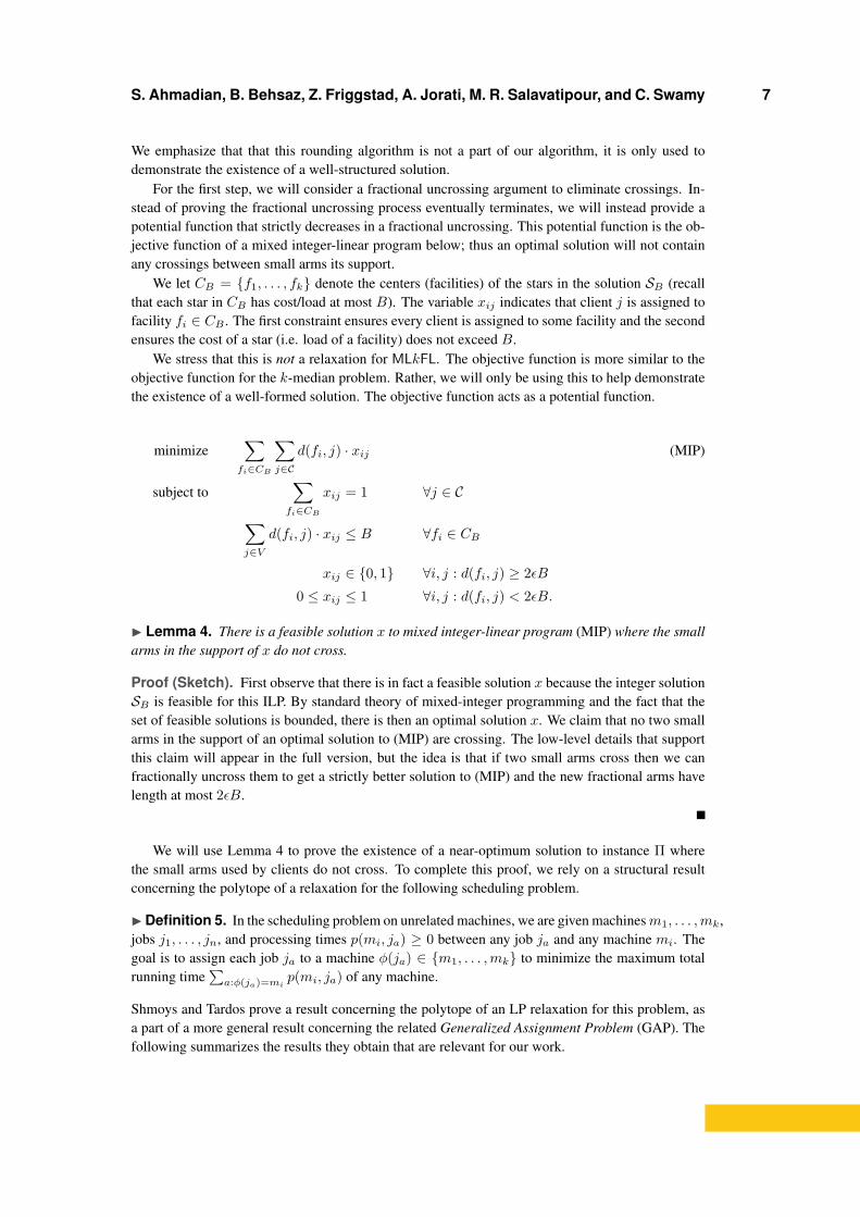
We let CB = f1, . . . , fk denote the centers (facilities) of the stars in the solution SB (recallthat each star in CB has cost/load at most B). The variable xij indicates that client j is assigned tofacility fi ∈ CB . The first constraint ensures every client is assigned to some facility and the secondensures the cost of a star (i.e. load of a facility) does not exceed B.

We stress that this is not a relaxation for MLkFL. The objective function is more similar to theobjective function for the k-median problem. Rather, we will only be using this to help demonstratethe existence of a well-formed solution. The objective function acts as a potential function.

minimize∑fi∈CB

∑j∈C

d(fi, j) · xij (MIP)

subject to∑fi∈CB

xij = 1 ∀j ∈ C

∑j∈V

d(fi, j) · xij ≤ B ∀fi ∈ CB

xij ∈ 0, 1 ∀i, j : d(fi, j) ≥ 2εB0 ≤ xij ≤ 1 ∀i, j : d(fi, j) < 2εB.

I Lemma 4. There is a feasible solution x to mixed integer-linear program (MIP) where the smallarms in the support of x do not cross.

Proof (Sketch). First observe that there is in fact a feasible solution x because the integer solutionSB is feasible for this ILP. By standard theory of mixed-integer programming and the fact that theset of feasible solutions is bounded, there is then an optimal solution x. We claim that no two smallarms in the support of an optimal solution to (MIP) are crossing. The low-level details that supportthis claim will appear in the full version, but the idea is that if two small arms cross then we canfractionally uncross them to get a strictly better solution to (MIP) and the new fractional arms havelength at most 2εB.

We will use Lemma 4 to prove the existence of a near-optimum solution to instance Π wherethe small arms used by clients do not cross. To complete this proof, we rely on a structural resultconcerning the polytope of a relaxation for the following scheduling problem.

IDefinition 5. In the scheduling problem on unrelated machines, we are given machinesm1, . . . ,mk,jobs j1, . . . , jn, and processing times p(mi, ja) ≥ 0 between any job ja and any machine mi. Thegoal is to assign each job ja to a machine φ(ja) ∈ m1, . . . ,mk to minimize the maximum totalrunning time

∑a:φ(ja)=mi p(mi, ja) of any machine.

Shmoys and Tardos prove a result concerning the polytope of an LP relaxation for this problem, asa part of a more general result concerning the related Generalized Assignment Problem (GAP). Thefollowing summarizes the results they obtain that are relevant for our work.

8 Approximation Algorithms for Minimum-Load k-Facility Location

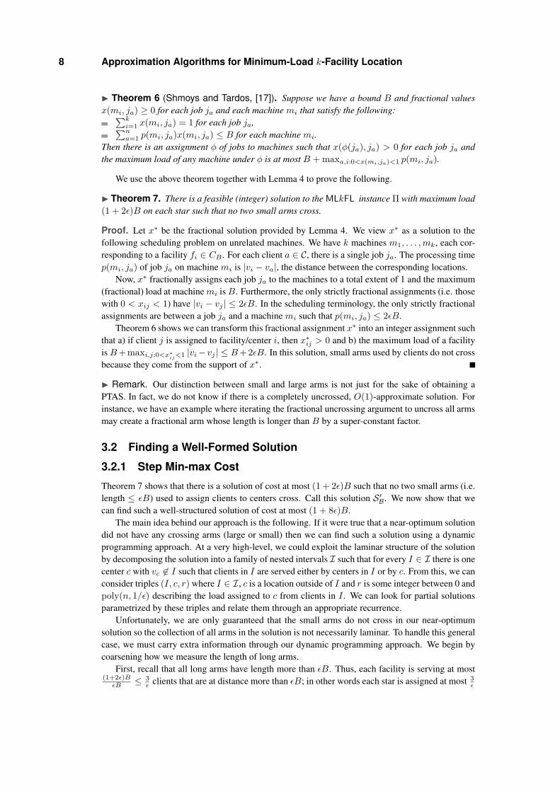
I Theorem 6 (Shmoys and Tardos, [17]). Suppose we have a bound B and fractional valuesx(mi, ja) ≥ 0 for each job ja and each machine mi that satisfy the following:∑k

i=1 x(mi, ja) = 1 for each job ja,∑na=1 p(mi, ja)x(mi, ja) ≤ B for each machine mi.

Then there is an assignment φ of jobs to machines such that x(φ(ja), ja) > 0 for each job ja andthe maximum load of any machine under φ is at most B + maxa,i:0<x(mi,ja)<1 p(mi, ja).

We use the above theorem together with Lemma 4 to prove the following.

I Theorem 7. There is a feasible (integer) solution to the MLkFL instance Π with maximum load(1 + 2ε)B on each star such that no two small arms cross.

Proof. Let x∗ be the fractional solution provided by Lemma 4. We view x∗ as a solution to thefollowing scheduling problem on unrelated machines. We have k machines m1, . . . ,mk, each cor-responding to a facility fi ∈ CB . For each client a ∈ C, there is a single job ja. The processing timep(mi, ja) of job ja on machine mi is |vi − va|, the distance between the corresponding locations.

Now, x∗ fractionally assigns each job ja to the machines to a total extent of 1 and the maximum(fractional) load at machinemi isB. Furthermore, the only strictly fractional assignments (i.e. thosewith 0 < xij < 1) have |vi − vj | ≤ 2εB. In the scheduling terminology, the only strictly fractionalassignments are between a job ja and a machine mi such that p(mi, ja) ≤ 2εB.

Theorem 6 shows we can transform this fractional assignment x∗ into an integer assignment suchthat a) if client j is assigned to facility/center i, then x∗ij > 0 and b) the maximum load of a facilityis B+ maxi,j:0<x∗

ij<1 |vi−vj | ≤ B+ 2εB. In this solution, small arms used by clients do not cross

because they come from the support of x∗.

I Remark. Our distinction between small and large arms is not just for the sake of obtaining aPTAS. In fact, we do not know if there is a completely uncrossed, O(1)-approximate solution. Forinstance, we have an example where iterating the fractional uncrossing argument to uncross all armsmay create a fractional arm whose length is longer than B by a super-constant factor.

3.2 Finding a Well-Formed Solution

3.2.1 Step Min-max Cost

Theorem 7 shows that there is a solution of cost at most (1 + 2ε)B such that no two small arms (i.e.length ≤ εB) used to assign clients to centers cross. Call this solution S ′B. We now show that wecan find such a well-structured solution of cost at most (1 + 8ε)B.

The main idea behind our approach is the following. If it were true that a near-optimum solutiondid not have any crossing arms (large or small) then we can find such a solution using a dynamicprogramming approach. At a very high-level, we could exploit the laminar structure of the solutionby decomposing the solution into a family of nested intervals I such that for every I ∈ I there is onecenter c with vc 6∈ I such that clients in I are served either by centers in I or by c. From this, we canconsider triples (I, c, r) where I ∈ I, c is a location outside of I and r is some integer between 0 andpoly(n, 1/ε) describing the load assigned to c from clients in I . We can look for partial solutionsparametrized by these triples and relate them through an appropriate recurrence.

Unfortunately, we are only guaranteed that the small arms do not cross in our near-optimumsolution so the collection of all arms in the solution is not necessarily laminar. To handle this generalcase, we must carry extra information through our dynamic programming approach. We begin bycoarsening how we measure the length of long arms.

First, recall that all long arms have length more than εB. Thus, each facility is serving at most(1+2ε)BεB ≤ 3

ε clients that are at distance more than εB; in other words each star is assigned at most 3ε

S. Ahmadian, B. Behsaz, Z. Friggstad, A. Jorati, M. R. Salavatipour, and C. Swamy 9

long arms in the solution provided by Theorem 7. Say that one such long arm is between client j andcenter i. If we moved both j and i left to their nearest integer multiples of ε2B, then their distancechanges by at most ε2B. If this is done for all long arms assigned to a center i, then the total load ofcenter i due to long arms changes by at most 3εB.

Now, notice that this way to measure the distance between client j and center i is simply ε2Btimes the number of integer multiples of ε2B that lie in the half-open interval (vi, vj ] if vi <vj or (vj , vi] if vj < vi. In the dynamic programming algorithm described below, we will usethis coarse method to measure the distance of long arms and call this the perceived cost of thestar. More specifically, the perceived cost of a star (f, S) is the total cost of the small arms plus∑j∈S:If,j long |v′′f − v′′j | where v′′i is the nearest multiple of ε2B to the left of vi. The following is

proved using arguments similar to the proof of Lemma 3, recalling that every star in S ′B has at most3/ε long arms.

I Lemma 8. The perceived cost of every star in S ′B is at most (1 + 5ε)B. Furthermore, any starwith perceived cost at most (1+5ε)B and at most 3/ε long arms has (actual) cost at most (1+8ε)B.

Our dynamic programming algorithm will find a solution with perceived cost at most (1 + 5ε)Band at most 3/ε large arms per star, so the actual cost will be at most (1 + 8ε)B.

3.2.2 Dynamic Programming

Before we formally define the subproblems of dynamic programming, we discuss the structure of awell-formed solution, say S. We call a client covered by a small (large) arm a small client (largeclient), respectively. Let the small span or s-span of a star be the interval, possibly empty, formedfrom the left most to the right most small client in this star. Since the small arms do not intersect inS, for any two s-spans I1 and I2 of two stars, either I1 ∩ I2 = ∅ or I1 ⊆ I2 or I2 ⊆ I1. Therefore,the ⊆ relation between s-span of stars in S defines a laminar family (a forest like structure).

Also, consider the restriction of S to the interval Ii,j for two arbitrary points vi and vj . Assumethat an arm has a direction and goes from the center of the star (i.e. the facility) to the client that itcovers. There are some large arms that enter or leave this interval from vi or vj . There are two typesof arms: the arms that enter the interval Ii,j from vi or vj or the arms that leave the interval Ii,j fromvi or vj ; for example a center inside the interval Ii,j might cover a client outside this interval or acenter to the left of i might cover a client inside the interval or a client to the right of j. Note thata large arm may have both these types, i.e., it enters from one endpoint and leaves from the otherendpoint. The arms that enter the interval can cover the deficiency of coverage for some client in theinterval and the arms that leave the interval provide coverage for some client outside of interval andcan be viewed as surplus to the demand of coverage of the clients in the interval. Also, recall thatin the perceived cost, the length of a large arm is measured as an integer multiple q of ε2B, where0 ≤ q ≤ 1

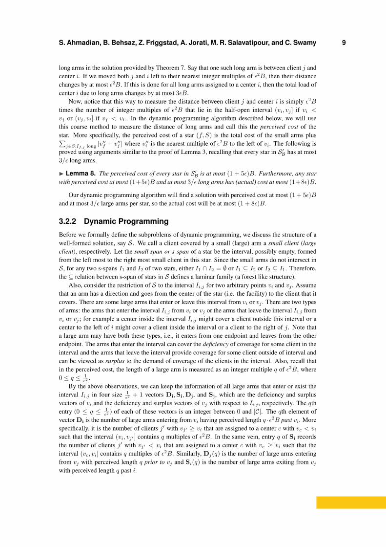
ε2 .By the above observations, we can keep the information of all large arms that enter or exist the

interval Ii,j in four size 1ε2 + 1 vectors Di,Si,Dj, and Sj, which are the deficiency and surplus

vectors of vi and the deficiency and surplus vectors of vj with respect to Ii,j , respectively. The qthentry (0 ≤ q ≤ 1

ε2 ) of each of these vectors is an integer between 0 and |C|. The qth element ofvector Di is the number of large arms entering from vi having perceived length q ·ε2B past vi. Morespecifically, it is the number of clients j′ with vj′ ≥ vi that are assigned to a center c with vc < visuch that the interval (vi, vj′ ] contains q multiples of ε2B. In the same vein, entry q of Si recordsthe number of clients j′ with vj′ < vi that are assigned to a center c with vc ≥ vi such that theinterval (vc, vi] contains q multiples of ε2B. Similarly, Dj(q) is the number of large arms enteringfrom vj with perceived length q prior to vj and Si(q) is the number of large arms exiting from vjwith perceived length q past i.

10 Approximation Algorithms for Minimum-Load k-Facility Location

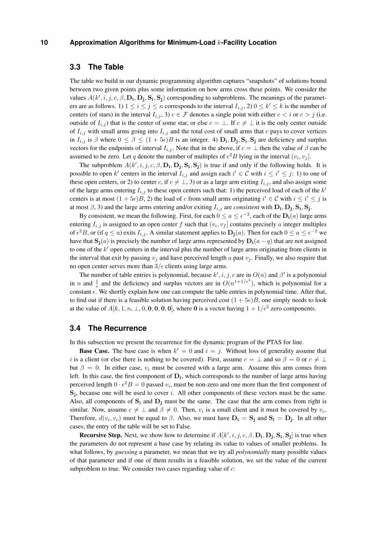
3.3 The Table

The table we build in our dynamic programming algorithm captures “snapshots” of solutions boundbetween two given points plus some information on how arms cross these points. We consider thevalues A(k′, i, j, c, β,Di,Dj,Si,Sj) corresponding to subproblems. The meanings of the paramet-ers are as follows. 1) 1 ≤ i ≤ j ≤ n corresponds to the interval Ii,j , 2) 0 ≤ k′ ≤ k is the number ofcenters (of stars) in the interval Ii,j , 3) c ∈ F denotes a single point with either c < i or c > j (i.e.outside of Ii,j) that is the center of some star, or else c = ⊥. If c 6= ⊥ it is the only center outsideof Ii,j with small arms going into Ii,j and the total cost of small arms that c pays to cover verticesin Ii,j is β where 0 ≤ β ≤ (1 + 5ε)B is an integer. 4) Di,Dj,Si,Sj are deficiency and surplusvectors for the endpoints of interval Ii,j . Note that in the above, if c = ⊥ then the value of β can beassumed to be zero. Let q denote the number of multiples of ε2B lying in the interval (vi, vj ].

The subproblem A(k′, i, j, c, β,Di,Dj,Si,Sj) is true if and only if the following holds. It ispossible to open k′ centers in the interval Ii,j and assign each i′ ∈ C with i ≤ i′ ≤ j: 1) to one ofthese open centers, or 2) to center c, if c 6= ⊥, 3) or as a large arm exiting Ii,j , and also assign someof the large arms entering Ii,j to these open centers such that: 1) the perceived load of each of the k′

centers is at most (1 + 5ε)B, 2) the load of c from small arms originating i′ ∈ C with i ≤ i′ ≤ j isat most β, 3) and the large arms entering and/or exiting Ii,j are consistent with Di,Dj,Si,Sj.

By consistent, we mean the following. First, for each 0 ≤ a ≤ ε−2, each of the Di(a) large armsentering Ii,j is assigned to an open center f such that (vi, vf ] contains precisely a integer multiplesof ε2B, or (if q ≤ a) exits Ii,j . A similar statement applies to Dj(a). Then for each 0 ≤ a ≤ ε−2 wehave that Sj(a) is precisely the number of large arms represented by Di(a− q) that are not assignedto one of the k′ open centers in the interval plus the number of large arms originating from clients inthe interval that exit by passing vj and have perceived length a past vj . Finally, we also require thatno open center serves more than 3/ε clients using large arms.

The number of table entries is polynomial, because k′, i, j, c are in O(n) and β′ is a polynomialin n and 1

ε and the deficiency and surplus vectors are in O(n1+1/ε2), which is polynomial for aconstant ε. We shortly explain how one can compute the table entries in polynomial time. After that,to find out if there is a feasible solution having perceived cost (1 + 5ε)B, one simply needs to lookat the value of A[k, 1, n,⊥, 0,0,0,0,0], where 0 is a vector having 1 + 1/ε2 zero components.

3.4 The Recurrence

In this subsection we present the recurrence for the dynamic program of the PTAS for line.Base Case. The base case is when k′ = 0 and i = j. Without loss of generality assume that

i is a client (or else there is nothing to be covered). First, assume c = ⊥ and so β = 0 or c 6= ⊥but β = 0. In either case, vi must be covered with a large arm. Assume this arm comes fromleft. In this case, the first component of Di, which corresponds to the number of large arms havingperceived length 0 · ε2B = 0 passed vi, must be non-zero and one more than the first component ofSj, because one will be used to cover i. All other components of these vectors must be the same.Also, all components of Si and Dj must be the same. The case that the arm comes from right issimilar. Now, assume c 6= ⊥ and β 6= 0. Then, vi is a small client and it must be covered by vc.Therefore, d(vi, vc) must be equal to β. Also, we must have Di = Sj and Si = Dj. In all othercases, the entry of the table will be set to False.

Recursive Step. Next, we show how to determine if A[k′, i, j, c, β,Di,Dj,Si,Sj] is true whenthe parameters do not represent a base case by relating its value to values of smaller problems. Inwhat follows, by guessing a parameter, we mean that we try all polynomially many possible valuesof that parameter and if one of them results in a feasible solution, we set the value of the currentsubproblem to true. We consider two cases regarding value of c:

S. Ahmadian, B. Behsaz, Z. Friggstad, A. Jorati, M. R. Salavatipour, and C. Swamy 11

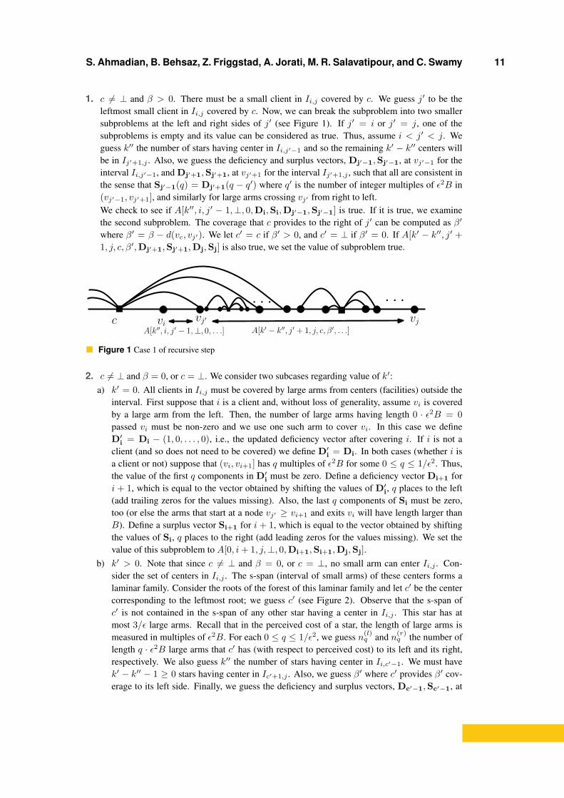
1. c 6= ⊥ and β > 0. There must be a small client in Ii,j covered by c. We guess j′ to be theleftmost small client in Ii,j covered by c. Now, we can break the subproblem into two smallersubproblems at the left and right sides of j′ (see Figure 1). If j′ = i or j′ = j, one of thesubproblems is empty and its value can be considered as true. Thus, assume i < j′ < j. Weguess k′′ the number of stars having center in Ii,j′−1 and so the remaining k′ − k′′ centers willbe in Ij′+1,j . Also, we guess the deficiency and surplus vectors, Dj′−1,Sj′−1, at vj′−1 for theinterval Ii,j′−1, and Dj′+1,Sj′+1, at vj′+1 for the interval Ij′+1,j , such that all are consistent inthe sense that Sj′−1(q) = Dj′+1(q − q′) where q′ is the number of integer multiples of ε2B in(vj′−1, vj′+1], and similarly for large arms crossing vj′ from right to left.We check to see if A[k′′, i, j′ − 1,⊥, 0,Di,Si,Dj′−1,Sj′−1] is true. If it is true, we examinethe second subproblem. The coverage that c provides to the right of j′ can be computed as β′

where β′ = β − d(vc, vj′). We let c′ = c if β′ > 0, and c′ = ⊥ if β′ = 0. If A[k′ − k′′, j′ +1, j, c, β′,Dj′+1,Sj′+1,Dj,Sj] is also true, we set the value of subproblem true.

c vjvi

. . .vj′

. . .

A[k′ − k′′, j′ + 1, j, c, β′, . . .]A[k′′, i, j′ − 1,⊥, 0, . . .]

Figure 1 Case 1 of recursive step

2. c 6= ⊥ and β = 0, or c = ⊥. We consider two subcases regarding value of k′:a) k′ = 0. All clients in Ii,j must be covered by large arms from centers (facilities) outside the

interval. First suppose that i is a client and, without loss of generality, assume vi is coveredby a large arm from the left. Then, the number of large arms having length 0 · ε2B = 0passed vi must be non-zero and we use one such arm to cover vi. In this case we defineD′i = Di − (1, 0, . . . , 0), i.e., the updated deficiency vector after covering i. If i is not aclient (and so does not need to be covered) we define D′i = Di. In both cases (whether i isa client or not) suppose that (vi, vi+1] has q multiples of ε2B for some 0 ≤ q ≤ 1/ε2. Thus,the value of the first q components in D′i must be zero. Define a deficiency vector Di+1 fori + 1, which is equal to the vector obtained by shifting the values of D′i, q places to the left(add trailing zeros for the values missing). Also, the last q components of Si must be zero,too (or else the arms that start at a node vj′ ≥ vi+1 and exits vi will have length larger thanB). Define a surplus vector Si+1 for i + 1, which is equal to the vector obtained by shiftingthe values of Si, q places to the right (add leading zeros for the values missing). We set thevalue of this subproblem to A[0, i+ 1, j,⊥, 0,Di+1,Si+1,Dj,Sj].

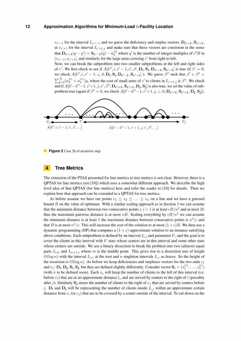
b) k′ > 0. Note that since c 6= ⊥ and β = 0, or c = ⊥, no small arm can enter Ii,j . Con-sider the set of centers in Ii,j . The s-span (interval of small arms) of these centers forms alaminar family. Consider the roots of the forest of this laminar family and let c′ be the centercorresponding to the leftmost root; we guess c′ (see Figure 2). Observe that the s-span ofc′ is not contained in the s-span of any other star having a center in Ii,j . This star has atmost 3/ε large arms. Recall that in the perceived cost of a star, the length of large arms ismeasured in multiples of ε2B. For each 0 ≤ q ≤ 1/ε2, we guess n(l)

q and n(r)q the number of

length q · ε2B large arms that c′ has (with respect to perceived cost) to its left and its right,respectively. We also guess k′′ the number of stars having center in Ii,c′−1. We must havek′ − k′′ − 1 ≥ 0 stars having center in Ic′+1,j . Also, we guess β′ where c′ provides β′ cov-erage to its left side. Finally, we guess the deficiency and surplus vectors, Dc′−1,Sc′−1, at

12 Approximation Algorithms for Minimum-Load k-Facility Location

vc′−1 for the interval Ii,c′−1 and we guess the deficiency and surplus vectors, Dc′+1,Sc′+1,at vc′+1 for the interval Ic′+1,j and make sure that these vectors are consistent in the sensethat Dc′+1(q − q′) = Sc′−1(q)− n(l)

q where q′ is the number of integer multiples of ε2B in(vc′−1, vc′+1], and similarly for the large arms crossing c′ from right to left.Now, we can break the subproblem into two smaller subproblems at the left and right sidesof c′. We first check to see if A[k′′, i, c′ − 1, c′, β′,Di,Si,Dc′−1,Sc′−1] is true (if β′ = 0,we check A[k′′, i, c′ − 1,⊥, 0,Di,Si,Dc′−1,Sc′−1] ). We guess β′′ such that β′ + β′′ +∑ 1

ε2q=0(n(l)

q + n(r)q )q, where the cost of small arms of c′ to clients in Ic′+1,j is β′′. We check

and ifA[k′−k′′−1, c′+1, j, c′, β′′,Dc′+1,Sc′+1,Dj,Sj] is also true, we set the value of sub-problem true (again if β′′ = 0, we checkA[k′−k′′−1, c′+1, j,⊥, 0,Dc′+1,Sc′+1,Dj,Sj]).

c′ vjvi

. . . . . .. . . . . .

A[k′ − k′′ − 1, c′ + 1, j, c′, β′′, . . .]A[k′′, i, c′ − 1, c′, β′, . . .]

Figure 2 Case 2b of recursive step

4 Tree Metrics

The extension of the PTAS presented for line metrics to tree metrics is not clear. However, there is aQPTAS for line metrics (see [10]) which uses a somewhat different approach. We describe the highlevel idea of that QPTAS (for line metrics) here and refer the reader to [10] for details. Then weexplain how that approach can be extended to a QPTAS for tree metrics.

As before assume we have our points v1 ≤ v2 ≤ . . . ≤ vn on a line and we have a guessedbound B on the value of optimum. With a similar scaling approach as in Section 3 we can assumethat the minimum distance between two consecutive points i, i+ 1 is at least εB/n2 and at most B;thus the maximum pairwise distance is at most nB. Scaling everything by εB/n2 we can assumethe minimum distance is at least 1 the maximum distance between consecutive points is n3/ε andthat B is at most n4/ε. This will increase the cost of the solution to at most (1 + ε)B. We then use adynamic programming (DP) that computes a (1 + ε)-approximate solution to an instance satisfyingabove conditions. Each subproblem is defined by an interval Ii,j and parameter k′, and the goal is tocover the clients in this interval with k′ stars whose centers are in this interval and some other starswhose centers are outside. We use a binary dissection to break the problem into two (almost) equalparts Ii,m and Im+1,j where m is the middle point. This gives rise to a dissection tree of heightO(logn) with the interval I1,n at the root and n singleton intervals Ii,i as leaves. So the height ofthe recursion is O(logn). As before we keep deficiencies and surpluses vectors for the two ends viand vj : Di,Dj,Si,Sj, but they are defined slightly differently. Consider vector Si = (s(i)

1 , . . . , s(i)σ )

(with σ to be defined soon). Each sa will keep the number of clients to the left of this interval (i.e.before vi) that are at an approximate distance la and are served by centers to the right of i (possiblyafter j). Similarly Sj stores the number of clients to the right of vj that are served by centers beforej. Di and Dj will be representing the number of clients inside Ii,j within an approximate certaindistance from vi (or vj) that are to be covered by a center outside of the interval. To cut down on the

S. Ahmadian, B. Behsaz, Z. Friggstad, A. Jorati, M. R. Salavatipour, and C. Swamy 13

interface of an interval Ii,j with the rest of the line, we round up the surplus and deficiency lengths oneach of the right and left sides to the nearest power of (1 + ε′/ logn), for some ε′ depending on ε, ateach level of dissection. Thus, we only keep track of lengths la = (1 + ε′/ logn)a, a ∈ 1, . . . , σ.For instance, for Si = (s(i)

1 , . . . , s(i)σ ), s(i)

a will be the number of clients to the left of Ii,j thatare at (scaled up) distance (1 + ε′/ logn)a from i that are served by centers inside the intervalIi,j . So there will be σ = O(logn · logB/ε′) = O(log2 n/ε′) different lengths and as a result atmost nO(log2 n/ε′) different surplus and deficiency vectors. In this way, each arm of a star will bescaled up by a factor of at most (1 + ε′/ logn) at each level of DP computation (to account for therounding), and since the depth of recursion (dissection) is dlogne, this will result in an extra factorof (1 + ε′/ logn)dlogne ≤ (1 + ε) (for a suitable choice of ε′) over the entire length of each arm. Inother words, if a subproblem for an interval i, j and parameter k′ is feasible (with each star costingat most B) without rounding the lengths of deficiency and surplus vectors then the subproblem withrounded (up to nearest power of (1+ ε′/ logn)) lengths for deficiency and surplus vectors is feasibleif each star is allowed to have cost at most (1 + ε) ·B.

Each entry of the table represents a subproblem (i, j, k′,Di,Dj,Si,Sj), where:1. i, j represents the interval Ii,j .2. k′ is the number of centers to be opened from among the points in Ii,j .3. Di = (d(i)

1 , . . . , d(i)σ ) and Dj = (d(j)

1 , . . . , d(j)σ ) are the deficiency vectors on the left and right

sides of the interval Ii,j , respectively.4. Si = (s(i)

1 , . . . , s(i)σ ) and Sj = (s(j)

1 , . . . , s(j)σ ) are the surplus vectors on the left and right sides

of Ii,j , respectively.

Each surplus and deficiency vector is a vector of size σ = O(log2 n/ε′), where d(p)a or s(p)

a (forp ∈ i, j) is the number of broken arm parts of length (1 + ε′/ logn)a (after rounding). Each entryof the table records in Boolean values the feasibility of having k′ stars centered in the points in Ii,j ,such that each star has cost at most (1 + ε) ·B. Each of the k′ stars would cover some clients in Ii,jand the clients located at distances Si and Sj from the endpoints i and j of the interval. The rest ofthe clients have to be covered with the broken arms of Di and Dj, thus connected to the two sides iand j, respectively. The size of the DP table is O(n2 · k · nO(logn logB/ε′)) = nO(log2 n/ε′), which isquasi-polynomial in n. See [10] for the details of how to fill in the entries of this table.

Now suppose that the given metric for the MLkFL instance can be represented as a cost functionon the edges of a tree T . The algorithm, as before, works with a guessed value B as an upper boundfor Lopt . Also, using a scaling argument as for the case of line metrics, we can assume that theaspect ratio of heaviest to cheapest edge cost is polynomially bounded. Next, we can make the treeT binary by introducing zero-cost edges at nodes that have more than two children, keeping one ofits children and placing the rest as a subtree hanging from the zero-cost edge added. Repeating thisgives a binary tree that still has linear size. So for the rest of this section we assume that the inputtree is binary.

For each binary tree with n nodes one can find an edge e = (u, v) (where u is parent of v)such that each subtree resulted by deleting e has size in [n/3, 2n/3]. This splitting of the tree intotwo subtrees Tv (tree rooted at v) and T \ Tv that are almost the same size (by a factor of at mosttwo) plays the role breaking the problem into two almost equal sizes. Given a binary tree T wecan recursively partition it into two “almost equal” subtrees until we arrive at subtrees of size 1.The depth of this recursive dissection will be O(logn) and each time we recursively break the treeinto two smaller binary trees (whose sizes differ by a factor of at most 2). The breaking pointintroduces a new interface (or “portal”) point for the two smaller sub-trees: if edge e = (u, v) iscut then v is an interface point (or portal) for the subproblem Tv in addition to any other interfacepoint it might have had passed on to from previous dissection operations, and u is an interfacepoint (portal) for T \ Tv in addition to any other portal points generated before. More specifically,

14 Approximation Algorithms for Minimum-Load k-Facility Location

each subproblem is of the form (T ′, k′, S(p)p∈P (T ′), D(p)p∈P (T ′)) where T ′ is a subtree that isobtained by performing the dissection operation, 0 ≤ k′ ≤ k is the number of centers of stars to beopened in T ′, P (T ′) ⊆ V (T ′) is the set of portal points of T ′. If a tree T is cut into two almostequal sized subtrees T1 (rooted at v) and T2 = T \ T1 by cutting edge e = (u, v) then P (T1) willconsist of all the portals of T that are in T1 plus node v. Similarly P (T2) consists of all the portalsof T that are in T2 plus node u. It follows that for each subproblem, the number of portals is at mostO(logn). The dynamic programming then follows along the same lines as the QPTAS describedabove (see [10] for details) for the line metrics, and we obtain the following theorem.

I Theorem 9. For any constant 0 < ε ≤ 1, there is a (1+ε)-approximation algorithm for MLkFLon tree metrics that runs in quasi-polynomial time.

4.1 Star metrics.

We now consider MLkFL in star metrics, but in the more-general setting where each client j has aninteger demand Dj that may be split integrally across various open facilities; we call this an integer-splittable assignment. The load of a facility i is now defined as

∑j xijd(i, j) where xij ∈ Z≥0

is the amount of j’s demand that is served by i. We devise a 14-approximation algorithm for thisproblem. At a high level our approach is similar to the one used to obtain the PTAS for line metrics.We again “guess” the optimal value B. We argue via a slightly different uncrossing technique thatif B ≥ Lopt , then there exists a well-structured fractional solution with maximum load at most6B, and use DP to obtain a fractional solution with maximum load at most 12B. This can thenbe converted to an integer-splittable assignment with maximum load at most 14B using the GAP-rounding algorithm, since it is easy to ensure via some preprocessing that d(i, j) ≤ 2B for everyfacility i and client j. Thus, we either determine that B < Lopt or obtain a solution with maximumload at most 14B. The details are deferred to the full version of this paper.

I Theorem 10. There is a 14-approximation algorithm for MLkFL on star metrics with non-uniform demands and integer-splittable assignments.

5 Hardness results and integrality-gap lower bounds

We now present various hardness and integrality-gap results. We prove that MLkFL is stronglyNP-hard on line metrics and APX-hard in the Euclidean plane (Theorems 11 and 12). We alsodemonstrate that a natural configuration-style LP has an unbounded integrality gap (Theorem 13).The details of the first two theorems are deferred to the full version of this paper.

I Theorem 11. Minimum-load k-facility location is strongly NP-hard even in line metrics.

I Theorem 12. It is NP-hard to α-approximate minimum-load k-facility location problem on theEuclidean plane, for any α < 4/3. Thus, MLkFL is APX-hard in the Euclidean plane.

5.1 Integrality-gap lower bound.

Let(F , C, d, k

)be an MLkFL instance. Given a candidate “guess” B of the optimal value, we

can consider the following LP-relaxation of the problem of determining if there is a solution withmaximum load at most B. We propose the following linear programming for the MLkFL . For eachfacility i ∈ F , define S(B; i) := C ⊆ C :

∑j∈C d(i, j) ≤ B to be the set of all stars centered at

i that induce load at most B at i. We will often refer to a star in S(B; i) as a configuration. (Notethat S(B; i) contains ∅.) Our LP Will be a configuration-style LP, where for every facility i and starC ∈ S(B; i), we have a variable denoting if star C is chosen for facility i. This yields the followingnatural feasibility LP.

S. Ahmadian, B. Behsaz, Z. Friggstad, A. Jorati, M. R. Salavatipour, and C. Swamy 15

∑i∈F

∑C∈S(B;i):j∈C

x(i, C) ≥ 1 ∀j ∈ C (1)

∑C∈S(B;i)

x(i, C) ≤ 1 ∀i ∈ F (2)

∑i∈F

∑C∈S(B;i)

x(i, C) ≤ k (3)

x ≥ 0.

(P)

Constraint (1) ensures that each client belongs to some configuration, and constraints (2) and (3)ensure that each facility belongs to at most one configuration, and that there are at most k configura-tions. We show that there is an MLkFL instance on the line metric, where the smallest value BLP forwhich (P) is feasible is smaller than the optimal value by an Ω(k/ log k) factor; thus, the “integralitygap” of (P) is Ω(k/ log k). Moreover, in this instance, the graph containing the (i, j) edges such thatd(i, j) ≤ BLP is connected.

I Theorem 13. The integrality gap of (P) is Ω(k/ log k) even for line metrics.

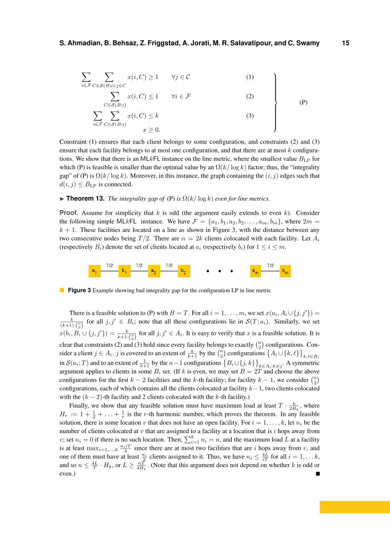
Proof. Assume for simplicity that k is odd (the argument easily extends to even k). Considerthe following simple MLkFL instance. We have F = a1, b1, a2, b2, . . . , am, bm, where 2m =k + 1. These facilities are located on a line as shown in Figure 3, with the distance between anytwo consecutive nodes being T/2. There are n = 2k clients colocated with each facility. Let Ai(respectively Bi) denote the set of clients located at ai (respectively bi) for 1 ≤ i ≤ m.

Figure 3 Example showing bad integrality gap for the configuration LP in line metric

There is a feasible solution to (P) withB = T . For all i = 1, . . . ,m, we set x(ai, Ai∪j, j′) =k

(k+1)·(n2) for all j, j′ ∈ Bi; note that all these configurations lie in S(T ; ai). Similarly, we set

x(bi, Bi ∪ j, j′) = k

k+1·(n2) for all j, j′ ∈ Ai. It is easy to verify that x is a feasible solution. It is

clear that constraints (2) and (3) hold since every facility belongs to exactly(n2)

configurations. Con-sider a client j ∈ Ai. j is covered to an extent of k

k+1 by the(n2)

configurationsAi∪k, `

k,`∈Bi

in S(ai;T ) and to an extent of 1k+1 by the n−1 configurations

Bi∪j, k

k∈Ai:k 6=j

. A symmetricargument applies to clients in some Bi set. (If k is even, we may set B = 2T and choose the aboveconfigurations for the first k − 2 facilities and the k-th facility; for facility k − 1, we consider

(n2)

configurations, each of which contains all the clients colocated at facility k−1, two clients colocatedwith the (k − 2)-th facility and 2 clients colocated with the k-th facility.)

Finally, we show that any feasible solution must have maximum load at least T · k2Hk , where

Hr := 1 + 12 + . . . + 1

r is the r-th harmonic number, which proves the theorem. In any feasiblesolution, there is some location v that does not have an open facility. For i = 1, . . . , k, let ni be thenumber of clients colocated at v that are assigned to a facility at a location that is i hops away fromv; set ni = 0 if there is no such location. Then,

∑ki=1 ni = n, and the maximum load L at a facility

is at least maxi=1,...,kniiT

4 since there are at most two facilities that are i hops away from v, andone of them must have at least ni2 clients assigned to it. Thus, we have ni ≤ 4L

iT for all i = 1, . . . k,and so n ≤ 4L

T ·Hk, or L ≥ nT4Hk . (Note that this argument does not depend on whether k is odd or

even.)

16 Approximation Algorithms for Minimum-Load k-Facility Location

6 Concluding Remarks

In this paper we present the first true polynomial time approximation for the MLkFL restricted toline metrics and the first true approximation in tree metrics. We also show that the standard toolsof LP rounding (even for configuration based LP) or local search methods, which have been usedsuccessfully for various facility location problems do not seem to work for this problem (even for thisrestricted metrics). Obviously, the major open question here is to obtain a true approximation (evenan O(logn)-approximation) for the MLkFL on general metrics. A smaller step could be to obtainsuch an algorithm for the Euclidean metrics. Note that the APX-hardness result for the Euclideanmetrics shows that this problem is significantly more difficult than the uncapacitated facility locationor k-median (for which there are known PTAS’s).

References

1 H.-C. An, A. Bhaskara, C. Chekuri, S. Gupta, V. Madan, and O. Svensson. Centrality of trees forcapacitated k-center. In Proceedings of APPROX, 2014.

2 E.M. Arkin, R. Hassin, and A. Levin. Approximations for minimum and min-max vehicle routingproblems. Journal of Algorithms, 59(1):1–18, 2006.

3 V. Arya, N. Garg, R. Khandekar, A. Meyerson, K. Munagala, and V. Pandit. Local search heuristicsfor k-median and facility location problems. SIAM Journal on Computing, 33(3):544–562, 2004.

4 M. Charikar, S. Guha, É. Tardos, and D. B. Shmoys. A constant-factor approximation algorithmfor the k-median problem. Journal of Computer and System Sciences, 65(1):129–149, 2002.

5 M. Cygan, M. T. Hajiaghayi, and S. Khuller. Lp rounding for k-centers with non-uniform hardcapacities. Arxiv preprint arXiv:1208.3054, 2012.

6 G. Even, N. Garg, J. Könemann, R. Ravi, and A. Sinha. Covering graphs using trees and stars. Ap-proximation, Randomization, and Combinatorial Optimization. Algorithms and Techniques, pages24–35, 2003.

7 D. Hochbaum and D. Shmoys. A polynomial approximation scheme for scheduling on uniformprocessors: using the dual approximation approach. SIAM Journal on Computing, 17:539–551,1988.

8 K. Jain, M. Mahdian, E. Markakis, A. Saberi, and V. V. Vazirani. Greedy facility location algorithmsanalyzed using dual-fitting with factor-revealing lp. Journal of the ACM, 50(6):795–824, 2003.

9 K. Jain and V. V. Vazirani. Approximation algorithms for metric facility location and k-medianproblems using the primal-dual schema and lagrangian relaxation. J. ACM, 48(2):274–296, 2001.

10 A. Jorati. Approximation algorithms for min-max vehicle routing problems. Master’s thesis, Uni-versity of Alberta, Department of Computing Science, 2013.

11 M. R. Khani and M. R. Salavatipour. Improved approximation algorithms for the min-max treecover and bounded tree cover problems. In APPROX, 2011.

12 S. Li and O. Svensson. Approximating k-median via pseudo-approximation. In Symposium onTheory of Computing (STOC), 2013.

13 P. Mirchandani and R. Francis, editors. Discrete location theory. Jown Wiley and Sons, 1990.14 H. Nagamochi and K. Okada. Approximating the minmax rooted-tree cover in a tree. Information

Processing Letters, 104(5):173–178, 2007.15 R. Ravi. Workshop on Flexible Network Design, 2012. http://fnd2012.mimuw.edu.pl/

qa/index.php?qa=4&qa_1=approximating-star-cover-problems.16 D. B. Shmoys. The design and analysis of approximation algorithms: facility location as a case

study. In S. Hosten, J. Lee, and R. Thomas, editors, Trends in Optimization, AMS Proceedings ofSymposia in Applied Mathematics 61, pages 85–97. 2004.

17 D. B. Shmoys and E. Tardos. An approximation algorithm for the generalized assignment problem.Mathematical Programming, 62(3):461–474, 1993.