FAST COLOR QUANTIZATION USING MACQUEEN’S K-MEANS

ALGORITHM

by

Skyler Thompson

A thesis presented to the Department of Computer Science and the Graduate School of the University of Central Arkansas

in partial fulfillment of the requirements for the degree of

Master of Science

in Computer Science

Conway, Arkansas May 2020

ProQuest Number:

All rights reserved

INFORMATION TO ALL USERSThe quality of this reproduction is dependent on the quality of the copy submitted.

In the unlikely event that the author did not send a complete manuscript and there are missing pages, these will be noted. Also, if material had to be removed,

a note will indicate the deletion.

Published by ProQuest LLC (

ProQuest

). Copyright of the Dissertation is held by the Author.

All Rights Reserved.This work is protected against unauthorized copying under Title 17, United States Code

Microform Edition © ProQuest LLC.

ProQuest LLC789 East Eisenhower Parkway

P.O. Box 1346Ann Arbor, MI 48106 - 1346

27744999

27744999

2020

TO THE OFFICE OF GRADUATE STUDIES:

The members of the Committee approve the thesis of

______________________________________ presented on

___________________________________________________________.

_______________________________________ Committee Chairperson

______________________________________ Committee Member

______________________________________ Committee Member

______________________________________ Committee Member

______________________________________ Committee Member

Skyler Thompson03/03/2020

M. Emre Celebi Digitally signed by M. Emre Celebi Date: 2020.03.21 10:48:41 -05'00'

Sinan Kockara Digitally signed by Sinan Kockara Date: 2020.03.23 15:49:33 -05'00'

Yu Sun Digitally signed by Yu Sun DN: cn=Yu Sun, o=University of Central Arkansas, ou=Computer Science Dept., email=yusun@uca.edu, c=US Date: 2020.03.23 16:31:32 -05'00'

iv

© 2020 Skyler Thompson

v

ACKNOWLEDGEMENT

I must first and foremost thank God for providing me with the knowledge and

guidance to get through my several years in college. After him, I must thank my wife for

her unwavering support throughout my college career. Of course, I cannot also forget my

family who have always been there through the good and the bad, encouraged me, and

provided both financial and emotional support throughout my life and college career.

I would also like to acknowledge Dr. Emre Celebi, professor and department chair

at the University of Central Arkansas. It is from him that the topic of this thesis and my

foreknowledge of data clustering stems. He was always available to respond to emails

and to help me through the difficult parts of both this paper and my research. Without

him, I never would have chosen to do a thesis and would have missed out on this entire

experience.

Finally, I would like to thank my boss, my supervisor, and my work colleagues.

Without their support and backing in my workplace, I never would have had the time to

dedicate to my research and to this thesis.

vi

ABSTRACT

Although not strictly necessary in all color image processing applications today,

color quantization still plays an important role in certain, typically hardware constrained,

applications. In this thesis, a novel color quantization method based on MacQueen’s k-

means algorithm, is proposed and compared to the more popular batch k-means

algorithm. The proposed method uses the maximin initialization method and quasi-

random sampling to achieve high quality, fast, and deterministic results. In comparison

to other well-known color quantization methods, the proposed method achieves very

competitive results while being much faster.

vii

TABLE OF CONTENTS

ACKNOWLEDGEMENT .................................................................................................. V

ABSTRACT ..................................................................................................................... VI

LIST OF TABLES ......................................................................................................... VIII

LIST OF FIGURES .......................................................................................................... IX

CHAPTER 1: INTRODUCTION ........................................................................................ 1

CHAPTER 2: RELATED WORK ...................................................................................... 3

CHAPTER 3: PROPOSED COLOR QUANTIZATION METHOD ................................. 7

CHAPTER 4: EXPERIMENTAL RESULTS AND DISCUSSION ................................. 13

CHAPTER 5: CONCLUSIONS AND FUTURE WORK ................................................ 31

REFERENCES .................................................................................................................. 33

viii

LIST OF TABLES

Table 1. Maximin Initialization Pseudocode ....................................................................... 8

Table 2. Batch K-Means Pseudocode ................................................................................ 10

Table 3. MacQueen’s K-Means Pseudocode ..................................................................... 10

Table 4. Test Images .......................................................................................................... 14

Table 5. Mean and Standard Deviation Ranks for Various Parameter Combinations ...... 17

Table 6. Comparison of Quantization Effectiveness ......................................................... 20

Table 7. Comparison of CPU Time ................................................................................... 21

ix

LIST OF FIGURES

Figure 1. Comparison of pseudo-random (a-c) and quasi-random (d-f) sampling ............ 12

Figure 2. Baboon output images (K = 32) ......................................................................... 25

Figure 3. Peppers output images (K = 64) ......................................................................... 26

Figure 4 Pills output images (K=128) ............................................................................... 27

Figure 5. Baboon error images (K=32) ............................................................................. 28

Figure 6. Peppers error images (K=64) ............................................................................. 29

Figure 7. Pills error images (K = 128) ............................................................................... 30

1

CHAPTER 1: INTRODUCTION

Pixels in an RGB image are comprised of three-color values: red, green, and blue.

RGB color images are then simply a rectangularly arranged collection of RGB triplets.

Because the red, green, and blue values can each range from 0 to 255, the total number

distinct colors that can be represented in a conventional 24-bit color image is 16,777,216.

This can be quite a lot of information, especially with larger, more complex images.

Therefore, the technique of color quantization (CQ) was conceived to help alleviate some

of the storage related constraints (Heckbert, 1982). Modern hardware can easily handle

these images, however there are still a large number of applications where CQ is used and

where advances in this field are quite useful.

Data Clustering

Data Clustering is a type of unsupervised learning (Celebi and Aydin, 2015) in

which data points are grouped into “clusters,” each of which is typically represented by a

center. Each cluster’s data points are typically similar to each other in some sense.

Various algorithms have been invented over the years for data clustering, with one of the

most popular algorithms being k-means and its numerous variants. K-means is a

partitional clustering method (Celebi, 2014) in which n observations are partitioned into k

clusters with each observation belonging to a single cluster.

In the context of CQ, clustering methods are typically divided into two different

categories: pre-clustering and post-clustering. Pre-clustering methods recursively find

nested clusters in either a divisive (top-down) or agglomerative (bottom-up) fashion. Pre-

clustering algorithms are typically faster than post-clustering algorithms and sacrifice

accuracy for speed. Post-clustering, on the other hand, find all k clusters simultaneously.

2

Color Quantization

CQ is a technique in which the number of colors in an input image is significantly

reduced by picking a predetermined number of colors from a palette and applying them to

all similarly colored pixels in the image (Braudaway, 1987). For example, if an original

image has around 100,000 colors, one may desire to reduce the number of colors to 64 in

order to achieve a faster and better compression. There have been several methods

devised for quantizing images over the past four decades (Heckbert, 1982) and among the

best of them is k-means. K-means clustering (Celebi, 2009; Celebi, 2011) is a natural

candidate because CQ can be viewed conveniently as a three-dimensional clustering

problem. Like nearly all post-clustering algorithms, this technique is typically performed

in two steps. The first is to choose the color palette, and the second is to map each of the

original pixels to the closest color in the palette.

3

CHAPTER 2: RELATED WORK

Several CQ techniques are used in the color image processing literature (Brun,

2002). Among them are: popularity (POP), median-cut (MC), modified popularity

(MPOP), octree (OCT), variance-based method (WAN), greedy orthogonal bipartitioning

(WU), center-cut (CC), self-organizing map (SOM), radius-weighted mean-cut (RWM),

modified maximin (MMM), pairwise clustering (PWC), split and merge (SAM), Cheng

and Yang (CY), fuzzy c-means (FCM), adaptive distributing units (ADU), and variance-

cut (VC).

Heckbert (1982) proposed the popularity method which builds a 16 x 16 x 16

color histogram using 4 bits per channel, and then takes the K most frequent colors in the

histogram as the color palette. He also proposed the median-cut method that builds a 32 x

32 x 32 color histogram containing pixel values reduced by uniform quantization to 5 bits

per channel. The histogram is split recursively into smaller boxes until K boxes are

obtained.

Braudaway (1987) introduced the modified popularity method that starts by

building a 2R x 2R x 2R histogram using R bits per channel. It chooses the most frequent

color as the first palette color and then reduces the frequency of each color. The

remaining colors are chosen in a similar fashion.

Gervautz and Purgathofer (1988) proposed the octree method which builds an

octree (tree data structure in which each internal node has up to eight children) that is a

representation of the input image color distribution. Then, it prunes the tree starting from

the bottom by merging nodes until K colors are obtained.

4

Wan, Prusinkiewicz, and Wong (1990) proposed the variance based method,

which is similar to Median-cut and starts the same but at each step, the box with the

largest square error is split along the principal axis at the point that minimizes marginal

weighted variance.

Wu (1991) proposed the greedy orthogonal bipartitioning procedure that is similar

to the variance-based method with the exception that at each step, the box with the largest

square error is split along the axis that minimizes the sum of the variance on both sides.

Joy and Xian (1993) proposed the center-cut method which is very similar to

median-cut except at each step, the box with the greatest range on any coordinate axis is

split along its longest axis at the mean point.

Dekker (1994) applied a one-dimensional self-organizing map (Kohonen, 1990)

to color quantization. A random subset of pixels is used in the training phase and the

final weights of the centers are taken as the color palette.

Yang and Lin (1996) proposed the radius-weighted mean-cut method that is

similar to the variance-based method, except the box is split along the vector from the

origin to the radius-weight mean at that point.

Xiang (1997) introduced the modified maximin method (Gonzalez, 1985) which

chooses the first center arbitrarily from the data set and the rest of the centers are chosen

to be the points with the largest minimum distance to the previously selected centers.

Each of the initially chosen centers are then recalculated as the mean of the points

assigned to them.

Velho, Gomez, and Sobreiro (1997) introduced the pairwise clustering method

that builds a 2R x 2R x 2R color histogram and controls a Q x Q joint quantization error

5

matrix where Q is the number of colors in the reduced color histogram. The clustering

procedure starts with Q singleton clusters, each of which contains one image color. In

each iteration, the pair of clusters with the least joint quantization error is merged (Ward,

1963). This process is repeated until K clusters remain.

Brun and Mokhtari (2000) created the split and merge method which first

partitions the color space into B partitions uniformly. This initial set is represented as an

adjacency graph. In the second (last) phase, B – K merge operations are performed to

obtain the final clusters (K). The pair of clusters with the minimum joint quantization

error are merged during the second phase.

Cheng and Yang (2001) created the method named after themselves, that is

similar to WAN, except at each step the box is split along a specially chosen line defined

by the mean color and the color that is farthest away at the mean point.

Wen and Celebi (2011) conducted a comparative study among several variants of

k-means and fuzzy c-means algorithms. They demonstrated that fuzzy c-means is

substantially slower than k-means and, in terms of quantization effectiveness, the former

algorithm is neither objectively nor subjectively superior to the latter.

Celebi (2014) introduced a CQ methods based the adaptive distributing units

algorithm (Uchiyama and Arbib, 1994). This algorithm is an online clustering algorithm

based on the competitive learning paradigm. What makes this postclustering method

interesting is that it does not require initialization.

Celebi, Wen, and Hwang (2015) developed the variance-cut method that is similar

to MC with the exception that, at each step, the box with the greatest SSE is split along

the coordinate axis with the greatest variance at the mean point. They also proposed the

6

variance-cut with Lloyd iterations method that is like VC except it locally optimizes the

two subpartitions resulting from each split using 10 Lloyd iterations.

7

CHAPTER 3: PROPOSED COLOR QUANTIZATION METHOD

This chapter serves to explain the proposed CQ method. The proposed method

starts by converting an image to a one-dimensional array of pixels (RGB values). Then,

it will initialize cluster centers using an appropriate adaptive method. After this, it will

begin to cluster the image by presenting pixels using a modified version of MacQueen’s

k-means algorithm. For each presented pixel, once it finds the closest center to the pixel,

it will immediately update this center. It will continue to do this until the cluster centers

do not move, or until a predetermined number of iterations is reached. Finally, once

MacQueen’s algorithm converges, each pixel in the input image is then mapped to its

nearest center.

Initialization

The simplest type of initialization is random selection. While random selection is

very efficient, it simply is not reliable enough to be used for this work (Celebi et al.,

2013). A common alternative to random selection is the maximin method of initialization

(Gonzalez, 1985). In the maximin method, the first center is chosen arbitrarily, and the

successive centers are chosen to be the point with the greatest minimum Euclidean

distance to the previously selected center. Euclidean distance between two RGB pixels

(R1, G1, B1) and (R2, G2, B2) is given by the equation

!(#! − #")! + ('! − '")! +()! − )")!. While it is typical to choose the first center

randomly, this essentially makes the entire method randomized. Instead, picking the

mean data point in the image as the starting point is a convenient and deterministic

approach, and the one used here. The pseudocode for maximin is given in Table 1.

8

Table 1. Maximin Initialization Method Pseudocode

Step Description

1 Take one center arbitrarily from the

dataset and make it the first center.

2

In iteration (i = 2, 3,…, K), the ith center

is chosen to be the one with the greatest minimum Euclidean distance to the

nearest previously selected (i−1) centers.

Lloyd’s Algorithm

Lloyd’s algorithm (Lloyd, 1982; Lindie et al., 1980) is one of the most common

clustering algorithms in scientific and engineering applications (Celebi et al., 2013).

Lloyd’s algorithm is commonly referred to as batch k-means and starts with a data set X =

{x1,…, xN} ⊆ RD and a positive integer value K, that is, the desired number of. For color

quantization purposes, N, D, and K correspond, respectively, to the number of pixels in

the input image, number of color channels (three in our case: RGB), and the number of

colors desired. The algorithm then assigns each data point to the closest cluster, thereby

minimizing the sum of error (SE) given by SE = ∑ ,(x, {0", … , 0#})$∈& , where

,(x, {0", … , 0#}) denotes the Bregman divergence of x to the nearest center in {c1,…,cK}.

Bregman divergences are a family of nonmetric dissimilarity functions including

Mahalanobis distance, Kullback-Leibler divergence, and Itakura-Saito divergence

(Banerjee et al., 2005). The most popular, and the one used in this case, is the squared

Euclidean distance. Because the squared Euclidean distance is used, the squared error SE

becomes the sum of squared error (SSE).

MacQueen’s Algorithm

An online formulation of the batch k-means algorithm was proposed by

MacQueen (MacQueen, 1967). It is similar to Lloyd’s algorithm in that each point is

9

assigned to the cluster that has the nearest center to that point (Thompson, 2020). The

two algorithms differ, however, in the way points are recomputed. Unlike the batch

algorithm, that updates all centers after the presentation of the entire set of points, the

online algorithm updates the nearest center after the presentation of each point. The

online algorithm can be viewed as an instance of the competitive learning paradigm

(Rumelhart and Zipser, 1985).

In a basic competitive learning algorithm, a randomly distributed set of units

compete for the right to respond to a subset of inputs (Rumelhart and Zipser, 1985).

After the presentation of each input, the unit that most closely resembles the input is the

winner and moves toward the input. This is termed “hard competitive learning” because

only the winner unit is adapted. Let x(t) be the input at time t (t = 1,2,…) and c(t) be the

corresponding nearest unit with respect to the ℓ2 distance. The adaptation equation for c(t)

is given by

0(()") = 0(() + η(()67(() − 0(()8,

where η∈ [0,1] is the learning rate, which is typically a monotonically decreasing

function of time. The larger the η value, the more emphasis given to new input and hence

the faster the learning. However, very large values of η may prevent the algorithm from

converging. In general, η is chosen to satisfy the Robbins-Monro conditions (Robbins-

Monro(1951):

lim(→-

η(=) = 0,

∑ η(t) = ∞-(." ,

10

∑ η(=)! < ∞-(." .

The conditions ensure that the learning rate decreases enough to suppress noise but not

too fast to avoid premature convergence. The pseudocodes for the batch and online

algorithms are given in Tables 2 and 3 respectively.

Table 2. Batch K-Means Algorithm Pseudocode

Step Description

1 Let {c1,…,cK} be the initial set of centers.

2 For each i ∈ {1,…, K}, set cluster Ci to be the set of points in X that are closer in

terms of d to ci than they are to any other center.

3 For each i ∈ {1,…, K}, set the center ci of cluster Ci to be the centroid of all points in

Ci.

4 Repeat Lloyd iterations (steps 2 and 3)

until convergence.

Table 3. MacQueen’s K-Means Algorithm Pseudocode

Step Description

1 Let {c1,…, cK} be the initial set of centers and n1 = … = nK = 1.

2 Select a random point xr from X and find the nearest center ci to this point.

3 Update the nearest center and the cardinality of the corresponding cluster

ci ← (nici+ xr)⁄(ni + 1),

ni ← ni + 1.

This ensures that the nearest center ci now accurately represents the mean of all

points in Ci.

4 Repeat steps 2 and 3 until convergence.

11

Presentation

Batch clustering algorithms, such as Lloyd’s algorithm, are less likely than online

algorithms such as MacQueen’s to escape poor local minima (Celebi, 2014). However,

online algorithms have two major drawbacks. First, stochastic selection of random input

data could potentially make each run generate different results, effectively randomizing

the output of the algorithm. Second, the presentation order matters and different orders

of presentation will result in different partitions. To solve this problem, quasi-random

sampling is used instead of pseudo-random sampling for the proposed method. A quasi-

random sequence differs from a pseudo-random sequence in that it fills the D-

dimensional Euclidean space RD more uniformly. Specifically, in this work, Sobol’

quasi-random sampling (Bratley and Fox, 1988) is used. Fig. 1 depicts three pseudo-

random sequences generated by the popular MT19937 generator (Matsumoto and

Nishimura, 1998) (top row) and three corresponding Sobol’ sequences (bottom row).

Because quasi-random sampling is deterministic, this method of sampling now makes the

modified MacQueen’s algorithm also deterministic.

12

Figure 1. Comparison of pseudo-random (a-c) and quasi-random (d-f) sampling

(a) Random sequence (210 pts)

(b) Random sequence (211 pts)

(c) Random sequence (212 pts)

(d) Sobol’ sequence (210 pts)

(e) Sobol’ sequence (211 pts)

(f) Sobol’ sequence (212 pts)

Color Quantization

After the method converges, we have a color palette (also known as a “color

map”). With the color palette at hand, we can start the actual CQ process. Every pixel

will be cycled through and compared against all of the cluster centers in order to find the

closest center to this pixel. After this, the pixels’ color values in the output image are

replaced by those of the closest center.

13

CHAPTER 4: EXPERIMENTAL RESULTS AND DISCUSSION

This chapter explains the experimental procedure, the results of the experiments,

and a discussion of the results. First, the test dataset used in the experiments is presented.

Next, the procedure used for the experiment is explained and the results are presented.

Finally, a detailed discussion of these results is provided.

Input Data

Table 4 presents the images used in the experiment, their name, file size, and

number of colors. These images are common in the CQ literature and present a diverse

amount of test data for the experiment. Note that both file size and the number of colors

is given because there is not a direct relationship between the two (i.e., a large file may

not necessarily have more colors). Baboon, Lenna, Peppers are from the USC-SIPI

Image Database; Motocross and Parrots are from the Kodak Lossless True Color Image

Suite; Goldhill, Fish, and Pills are by Lee Crocker, Luiz Velho, and Karel de Gendre. It

is worth noting that the images used in the experiment are binary PPM files (P6) and the

program developed for this thesis only accepts this specific format for reasons of

programmer convenience and portability.

14

Table 4. Test Images

Image Image Name File Size Num Colors

Baboon 997KB 230,427

Fish 228KB 28,170

Goldhill 1.6MB 90,966

15

Image Image Name File Size Num Colors

Lenna 997KB 148,279

Motocross 433KB 63,558

Parrots 324KB 72,079

Peppers 997KB 183,525

16

Image Image Name File Size Num Colors

Pills 1.6MB 206,609

Experimental Setup

There are three parameters that are tested in the presented CQ method. The first

is K, which is present in nearly all CQ methods. The second and third are the learning

rate (B ∈ (0.5,1]) and sampling fraction (f ∈ (0, 1]) respectively. The learning rate

controls the rate of adaptation and the sampling fraction controls the proportion of input

pixels that participate in the learning phase of MacQueen’s algorithm. Determining the

best possible parameter combination for this CQ method involved considering 24 distinct

possibilities: p ∈ {0.5, 0.6, 0.7, 0.8, 0.9, 1} × f ∈ {0.25, 0.5, 0.75, 1}. For each input

image and K ∈ {32, 64, 128, 256} value, each image was quantized using the CQ method

separately with each of the 24 combinations of (p, f) values. The computed Mean

Squared Error (MSE) between the input and output images was then taken. The MSE is

given by the mathematical formulation

MSE(X, XK) = "/0∑ ∑ |MN(ℎ, P) − NQ(ℎ, P)M|!!0

1."/2." ,

where X and XK denote, respectively, the H x W original and quantized images in the RGB

color space. These 24 MSE values were then ranked from best to worst, with the lowest

value being the best and the highest being the worst. Finally, the mean and standard

deviation of the MSE ranked values were calculated. These results are given in Table 5.

17

Table 5. Mean and Standard Deviation Ranks for Various Parameter Combinations

p f Mean Std

0.5 0.25 9.5 2.8

0.5 4.8 2.1

0.75 2.9 1.3

1.00 1.4 0.8

0.6 0.25 10.6 2.8

0.5 6.6 1.7

0.75 5.4 2.4

1.00 3.4 2.3

0.7 0.25 14.1 3.1

0.5 9.8 2.1

0.75 7.8 2.2

1.00 7.4 3.3

0.8 0.25 17.5 2.9

0.5 14.3 1.9

0.75 13.0 2.5

1.00 11.6 2.7

0.9 0.25 20.7 1.7

0.5 17.7 1.8

0.75 17.3 1.9

1.00 16.5 2.6

1.0 0.25 23.4 1.2

0.5 22.0 1.5

0.75 21.6 1.5

1.00 20.7 1.7

18

Comparison with Other CQ Methods

The proposed method is compared to the 15 well-known color quantization

methods described above: popularity (POP), median-cut (MC), modified popularity

(MPOP), octree (OCT), variance-based method (WAN), greedy orthogonal bipartitioning

(WU), center-cut (CC), radius-weighted mean-cut (RWM), pairwise clustering (PWC),

split and merge (SAM), Cheng and Yang (CY), variance-cut (VC), variance-cut with

Lloyd iterations (VCL), self-organizing map (SOM), and modified maximin (MMM).

Two variations of MacQueen’s and two variants of Lloyd’s (batch) k-means

algorithms were implemented for comparison. The two variations of batch (BKM) were

developed as an adaptation of Lloyd’s k-means clustering algorithm: One-pass BKM

(denoted by BKM1) and convergent BKM (denoted by BKM). One-pass BKM is nothing

but the batch version of MacQueen’s algorithm where the set of image pixels is presented

to the algorithm exactly once. Convergent BKM, on the other hand, performs Lloyd

iterations until cluster memberships of points no longer change. The two variations of

MacQueen’s algorithm are: one with pseudo-random sampling (denoted by MKMp) and

one with quasi-random sampling (denoted by MKMq). The pseudo-random sampling

variant uses the MT19937 (Mersenne Twister) generator. In each iteration, a pseudo-

random data point is presented to the algorithm by generating an unbiased pseudo-

random integer using a recent algorithm due to Lemire (2019). The quasi-random variant

of MacQueen’s algorithm uses a quasi-random sampling using a Sobol’ sequence. All

four k-means variant were initialized using the maximin method.

Table 6 compares the effectiveness, or quality, of the CQ methods. The best

(lowest) values are bolded for emphasis. For the only randomized color quantization

19

method, MKMq, the values are given in the format ms, where m and s are the mean and

standard deviation, respectively, over 100 independent runs.

20

Table 6. Comparison of Quantization Effectiveness CQ K K K K

32 64 128 256 32 64 128 256 32 64 128 256 32 64 128 256

Baboon Fish Goldhill Lenna

POP 1679.5 849.5 330.7 170.4 2827.6 482.5 105.2 69.8 576.7 199.3 101.8 73.1 347.2 199.5 84.5 65.3

MC 643.0 445.6 307.4 213.0 282.3 189.4 121.2 75.9 293.9 188.8 132.3 86.5 214.0 146.1 112.4 80.3

MPOP 453.1 290.4 195.0 109.3 198.4 145.5 66.2 47.7 200.2 140.7 66.7 48.6 194.5 138.9 60.0 47.8

OCT 530.2 306.6 203.6 125.0 218.4 125.1 77.8 44.3 230.3 130.3 79.0 45.7 186.7 110.0 66.0 40.6

WAN 528.3 385.7 266.0 178.0 311.6 209.0 124.5 77.1 229.0 141.2 94.5 64.4 216.5 140.8 87.6 56.7

WU 468.3 288.3 186.5 118.6 187.6 111.6 69.0 43.8 196.0 114.2 71.4 45.2 158.2 99.1 61.7 39.4

CC 473.1 299.7 202.5 144.7 189.8 127.3 82.3 56.5 202.0 134.9 87.9 57.9 189.1 125.5 80.6 52.2

RWM 459.0 301.6 188.1 120.2 176.7 109.0 68.9 44.4 179.8 118.3 71.0 44.5 161.2 94.6 60.1 39.2

PWC 469.4 308.8 206.7 128.8 201.5 130.9 93.1 69.4 193.8 125.1 88.9 70.9 186.9 108.0 78.8 65.0

SAM 464.9 293.9 188.8 119.8 198.5 120.1 74.0 48.5 179.3 111.2 70.4 46.7 158.0 102.0 65.0 45.4

CY 465.9 280.9 187.3 117.7 193.8 112.5 72.0 44.8 186.3 121.6 72.2 46.4 166.4 97.6 62.5 41.9

VC 450.6 273.5 179.9 117.6 168.1 106.5 67.4 43.4 174.8 109.5 68.3 42.4 145.6 91.7 60.7 38.9

VCL 425.6 264.0 173.1 115.3 169.9 102.5 65.1 43.1 169.3 104.3 66.2 42.0 146.3 89.2 59.2 38.6

SOM 433.6 268.9 163.9 108.2 180.4 114.1 60.4 45.1 182.1 104.2 59.5 38.4 140.2 87.4 50.5 33.9

MMM 510.0 368.4 230.4 147.5 223.4 144.2 81.7 53.7 239.9 143.1 95.4 61.0 183.3 114.2 73.5 48.5

BKM1 505.0 341.7 218.2 138.2 242.5 139.9 87.3 48.9 250.9 149.3 90.6 61.5 192.9 124.1 72.2 48.1

BKM 374.2 234.3 149.3 95.6 142.6 90.2 57.3 34.8 143.8 83.0 52.0 34.2 130.8 74.7 46.8 30.3

MKMp 375.31.4 236.4.6 152.2.3 98.2.2 147.93.1 93.31.1 59.5.5 37.0.3 144.4.7 84.1.5 53.3.2 35.6.2 131.3.5 75.2.3 47.7.2 31.4.1

MKMq 375.6 236.2 152.0 97.6 148.7 92.8 59.2 36.2 144.3 83.3 53.3 35.7 131.4 75.4 47.9 31.3

Motocross Parrots Peppers Pills

POP 1288.6 474.3 201.6 93.5 4086.8 371.7 180.6 104.0 1389.3 367.7 218.3 129.1 788.2 222.9 124.0 85.3

MC 437.6 254.0 169.4 114.3 441.0 265.1 153.6 112.3 377.6 238.9 173.8 121.9 324.2 233.8 159.5 100.4

MPOP 287.5 177.9 84.1 53.3 379.8 212.1 104.7 59.4 338.7 204.9 112.1 69.3 277.5 175.2 88.4 55.1

OCT 300.5 158.9 96.2 54.2 342.4 191.2 111.2 63.8 317.4 193.1 113.9 68.9 281.9 159.8 99.1 56.9

WAN 445.6 292.1 168.7 92.4 376.0 233.4 153.4 92.2 348.1 225.7 157.2 106.4 294.9 197.7 133.1 87.7

WU 268.1 147.2 86.7 51.0 299.2 167.3 95.4 58.3 278.9 165.5 102.2 66.1 261.2 150.1 89.5 55.0

CC 335.1 202.0 122.6 74.9 398.8 246.5 148.7 78.9 418.4 256.8 160.7 107.9 285.9 171.7 111.9 77.4

RWM 251.4 150.1 83.7 51.0 296.5 171.0 99.8 60.6 295.6 178.8 107.1 69.2 260.4 149.7 88.8 55.6

PWC 243.2 161.2 101.5 78.0 349.4 205.1 125.8 86.0 344.8 183.7 121.1 80.0 283.4 169.3 110.5 75.6

SAM 238.1 138.5 81.8 53.5 282.4 157.5 92.4 58.8 275.7 159.2 100.8 65.9 246.2 141.2 85.0 53.7

CY 248.0 146.6 89.3 53.0 313.2 178.6 106.7 64.5 317.3 186.1 114.1 72.6 237.8 157.9 96.4 58.8

VC 253.2 144.5 79.6 48.8 290.6 166.4 98.0 58.5 294.8 169.3 108.0 69.5 234.4 146.6 90.2 54.2

VCL 240.6 131.5 77.1 47.9 263.7 157.5 96.6 57.2 261.1 160.3 103.8 68.4 229.8 141.4 85.7 53.8

SOM 301.7 134.7 70.3 44.2 279.4 151.5 82.2 47.7 270.9 160.5 89.9 69.1 226.4 137.8 72.4 46.0

MMM 407.9 276.9 138.2 85.6 352.1 194.8 128.7 68.5 341.5 213.3 136.5 85.2 276.2 174.9 117.2 75.6

BKM1 389.4 237.8 166.2 85.7 363.7 202.1 121.3 71.6 363.1 232.2 138.7 92.8 307.5 188.3 121.5 72.0

BKM 197.5 115.0 68.0 42.9 230.7 129.5 73.2 44.3 248.7 148.1 87.7 55.0 198.4 111.1 66.3 41.0

MKMp 200.24.2 115.91.6 71.9.9 45.0.4 236.63.6 129.51.2 75.9.7 45.2.3 257.53.3 148.61.1 89.6.4 57.6.2 199.71.4 112.3.6 67.3.4 42.5.2

MKMqq 194.3 116.7 72.7 44.6 241.2 127.2 75.9 44.3 258.3 148.9 89.4 57.6 199.0 112.0 67.3 42.4

21

Table 7 compares the CPU time for the k-means based CQ methods on three of

the eight images. Because the three most effective CQ methods are consistently superior

to the others, they are the only ones compared in this experiment. They are compared on

the three most well-known images in CQ literature (Lenna, Baboon, and Peppers), with

each having the same resolution of 512 x 512 pixels. The remaining methods are left out

because they are either pre-clustering methods that sacrifice effectiveness for speed, or

post-clustering methods that do not perform particularly well. “Init” is the initialization

time (msec), “Clust” is the clustering time (msec), “cr” is the clustering time for BKM

divided by that for BKM, MKMp, or MKMq, and “tr” is the total time for BKM divided

by that for BKM, MKMp, or MKMq. All methods were implemented using the C

language with the gcc v8.2.0 compiler and the Intel Core i7-6700 (3.4GHz) processor.

The time figures were averaged over 100 independent runs.

Table 7. Comparison of CPU Time Image CQ 32 64 128 256

init clust cr tr init clust cr tr init clust cr tr init clust cr tr

Baboon BKM 39 4413 1 1 76 14249 1 1 146 27196 1 1 283 40378 1 1

MKMp 37 54 82 49 73 73 195 98 144 111 246 107 283 200 202 84

MKMq 37 64 69 44 73 83 171 92 144 122 223 103 283 200 202 84

Lenna BKM 38 4319 1 1 75 9259 1 1 147 26378 1 1 283 32952 1 1

MKMp 36 52 82 49 72 73 127 64 143 109 241 105 283 200 165 69

MKMq 36 63 68 44 72 84 111 60 143 122 217 100 283 200 165 69

Peppers BKM 36 2610 1 1 74 6259 1 1 147 33127 1 1 284 30275 1 1

MKMp 37 54 48 29 71 72 87 44 143 110 300 131 284 198 153 63

MKMq 36 63 41 27 72 83 76 41 143 122 272 126 284 198 153 63

22

Discussion of Results

For the presented CQ method, Table 3 (p,f) = (0.5, 1) is the best combination

attaining mean and standard deviation ranks of 1.4 and 0.8 respectively. This parameter

combination almost always generates the lowest distortion. Despite the fact that p = 1 is

the most common choice in the statistical literature, the experiments demonstrated that p

= 0.5 may be a better choice for finite data sets and K > 1. Table 3 shows that the mean

MSE ranks constantly decrease with increasing f. Given that typically the more input

pixels that are used, the better the learning for the dataset, this is not surprising. From a

theoretical and empirical perspective, the best parameter combination for the examined

CQ method is (p,f) = (0.5, 1).

Table 6, which compares the MSE of the different CQ methods shows several

interesting results:

• Interestingly, MKM performs either best or close to the best every time and

BKM1 performs among the worst, despite the fact that both make a single pass

over the image using almost the same operations. Both are also initialized with

maximin. The only explanation for this drastic performance difference is the

online nature of MKM, which helps it to easier escape from poor local minima

and learn faster.

• Post-clustering methods are more effective than pre-clustering methods in almost

all results, with VC and VCL performing better than the other pre-clustering

methods (VCL is not purely pre-clustering because it performs refinement using

Lloyd iterations after every split).

23

• Both the pseudo-random and quasi-random versions of MacQueen’s k-means

(MKMp and MKMq) have very similar effectiveness and in most cases, BKM is

slightly more effective than either variant. The differences in MSE are negligible,

however, and BKM only outperforms MKM by a few units.

Table 7, which compares the CPU time for each of the top three clustering methods

(BKM, MKMp, and MKMq) shows the following observations:

• By observing the total times ratios, one can see that MKMp is ever so slightly

faster than MKMq, because pseudo-random sampling is more efficient than

quasi-random sampling. This is a very small trade-off for a deterministic

scheme, however. Both methods are faster than BKM and the larger K

becomes, the faster the methods become in relation.

• Maximin exhibits linear behavior with respect to K. When K is increased, the

initialization time for MKM increases at the same rate (doubling each time K

does).

• BKM does not scale predictably. In some cases when doubling K, the

clustering time is increased by a factor of more than 5, whereas in other cases,

doubling K actually decreases clustering time. This is because that, for a

given image, the number of iterations for Lloyd’s algorithm cannot be

determined in advance and varies based on several factors including initial

centers and distribution of colors in the image.

• In BKM, initialization time is very small compared to clustering time. The

same cannot be said for MKM, which sometimes has the initialization phase

take longer than the clustering phase. A faster initialization method than

24

maximin can be used to help compensate for this but implementation

convenience and portability is sacrificed as a result.

• The image used makes a huge impact on the execution time of BKM. For

example, for K = 64, BKM takes ≈ 14.2s on Baboon, whereas clustering for

Peppers takes ≈ 6.3s. This is a huge difference and can be explained by the

amount of colors and the complexity of the image (higher complexity means

higher execution time).

Images Quantized Using Various CQ Methods

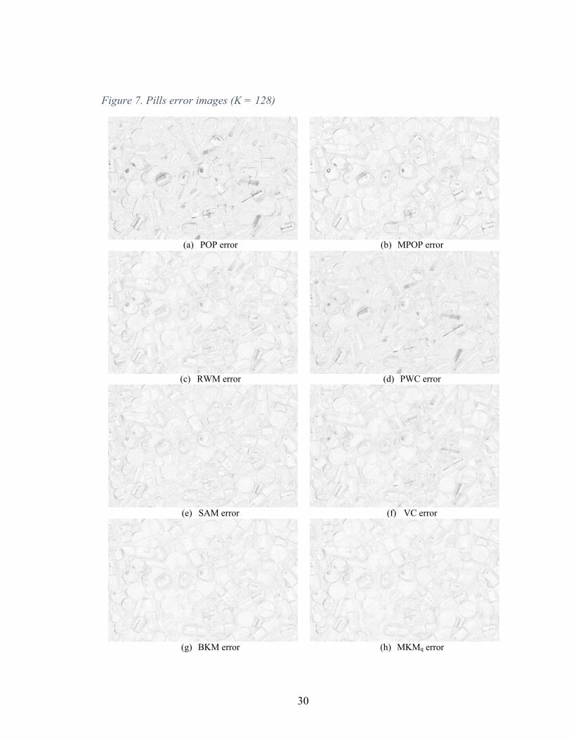
Figures 2 and 4 below show sample quantization results for close-up parts of

Baboon, Peppers, and Pills images. Figures 3 and 5 show the full-scale error images for

these images. The error image for a particular CQ method was obtained by taking the

pixelwise absolute difference between the original and quantized images. For better

visualization, pixel values of the error images were multiplied by 4 and then negated.

25

Figure 2. Baboon output images (K = 32)

(a) Original

(a) MC output

(c) WAN output

(d) OCT output

(e) VCL output

(f) SOM output

(g) MMM output

(h) BKM output

(i) MKMq output

26

Figure 3. Peppers output images (K = 64)

(a) Original

(b) MC output

(c) WAN output

(d) SAM output

(e) CY output

(f) VCL output

(g) SOM output

(h) BKM output

(i) MKMq output

27

Figure 4. Pills output images (K=128)

(a) Original

(b) POP output

(c) MPOP output

(d) RWM output

(e) PWC output

(f) SAM output

(g) VC output

(h) BKM output

(i) MKMq output

28

Figure 5. Baboon error images (K=32)

(a) MC error

(b) WAN error

(c) OCT error

(d) VCL error

(e) SOM error

(f) MMM error

(g) BKM error

(h) MKMq error

29

Figure 6. Peppers error images (K=64)

(a) MC error

(b) WAN error

(c) SAM error

(d) CY error

(e) VCL error

(f) SOM error

(g) BKM error

(h) MKMq error

30

Figure 7. Pills error images (K = 128)

(a) POP error

(b) MPOP error

(c) RWM error

(d) PWC error

(e) SAM error

(f) VC error

(g) BKM error

(h) MKMq error

31

CHAPTER 5: CONCLUSIONS AND FUTURE WORK

In this thesis, a variation of MacQueen’s online k-means algorithm was

introduced as a means to quantize color images. A series of experiments were performed

in order to determine the best parameter combination for the proposed algorithm.

Included within the tested algorithms, was both a pseudo-random and quasi-random

implementation of MacQueen’s k-means clustering algorithm. Both utilized maximin as

the initialization method due to its deterministic nature and superior results to that of

random selection. The pseudo-random implementation utilized the MT19937 generator

and the quasi-random implementation used the Sobol’ sequence. The results of the

experiment demonstrated that MacQueen’s algorithm was comparable to Lloyd’s

algorithm in effectiveness and was several times faster.

In the experiments, MacQueen’s algorithm was compared against a number of CQ

algorithms: popularity, median-cut, modified popularity, octree, variance-based method,

greedy orthogonal bipartitioning, center-cut, radius-weighted mean-cut, pairwise

clustering, split and merge, Cheng and Yang, variance-cut, variance-cut with Lloyd

iterations, self-organizing map, and modified maximin. Along with these were two

custom implementations of Lloyd’s algorithm. While Lloyd’s algorithm performed best

in nearly all scenarios, typically the resulting difference between it and MacQueen’s

algorithm was negligible. The primary difference between the two was speed.

MacQueen’s algorithm consistently performed many times faster than Lloyd’s due to its

online nature.

In this study, only maximin was used as an initialization method. Many other

initialization methods have been developed (Celebi et al., 2013), and through further

32

experimentation, perhaps faster and better results could be achieved. The quasi-random

variant of MacQueen’s algorithm was of particular interest during this study due to its

deterministic nature, and the only presentation method tested for this was the Sobol’

sequence. It would be interesting to compare other sampling methods (Ros and

Guillaume, 2020), such as coreset sampling (Valenzuela et al., 2018) to perhaps achieve

better results.

33

REFERENCES

Banerjee, A., Merugu, S., Dhillon, I., Ghosh, J. (2005). Clustering with Bregman

Divergences. Journal of Machine Learning Research 6, 1705–1749

Bratley, P., Fox, B.L. (1988). Algorithm 659: implementing Sobol’s quasi-random

sequence generator. ACM Transactions on Mathematical Software 14(1), 88–100

Braudaway, G. W. (1987). Procedure for Optimum Choice of a Small Number of Colors

from a Large Color Palette for Color Imaging. Proceedings of the Electronic

Imaging Conference, 71–75.

Brun, L., Mokhtari, M. (2000). Two High Speed Color Quantization Algorithms.

Proceedings of the 1st International Conference on Color in Graphics and Image

Processing, 116–121.

Brun, L., Trémeau, A. (2002). Color Quantization. Digital Color Imaging Handbook,

ppp. 589–638. CRC Press, Boca Raton

Celebi, M. E. (2009). Fast Color Quantization Using Weighted Sort-Means Clustering.

Journal of the Optical Society of America A, 26(11), 2434–2443. doi:

10.1364/JOSAA.26.002434

Celebi, M. E. (2011). Improving the Performance of K-Means for Color Quantization.

Image and Vision Computing, 29(1), 260–271. doi: 10.1016/j.imavis.2010.10.002

Celebi, M. E., Kingravi, H., and Vela, P. A. (2013). A Comparative Study of Efficient

Initialization Methods for the K-Means Clustering Algorithm. Expert Systems

with Applications, 40(1), 200–210. doi: 10.1016/j.eswa.2012.07.021

Celebi, M. E., Hwang, S and Wen, Q. (2014) Color Quantization Using the Adaptive

Distributing Units Algorithm. Imaging Science Journal, 62(2), pp. 80–91.

34

Celebi, M. E. (2014). Partitional Clustering Algorithms. Springer. doi: 10.1007/978-3-

319-09259-1

Celebi, M. E., Wen, Q., & Hwang, S. (2015). An Effective Real-Time Color Quantization

Methods Based on Divisive Hierarchical Clustering. Journal of Real-Time Image

Processing, 10(2), 329–344. doi: 10.1007/s11554-012-0291-4

Cheng, S., & Yang, C. (2001). Fast and Novel Technique for Color Quantization Using

Reduction of Color Space Dimensionality. Pattern Recognition Letters, 22(8),

845–856. doi: 10.1016/S0167-8655(01)00025-3

Gervautz, M., & Purgathofer, W. (1988). A Simple Method for Color Quantization:

Octree Quantization. In N. Magnenat-Thalmann & D. Thalmann (Eds.), New

Trends in Computer Graphics (pp. 219–231). Berlin, Germany: Springer. doi:

10.1007/978-3-642-83492-9_20

Gonzalez, T. F. (1985). Clustering to minimize the maximum interclustering distance.

Theoretical Computer Science. 18(2–3), 293–306

Heckbert, P. (1982). Color Image Quantization for Frame Buffer Display. Proceedings of

ACM SIGGRAPH Computer Graphics, 16(3), 297–307. doi:

10.1145/965145.801294

Kohonen, T. (1990). The self-organizing map. Proceedings of the IEEE. 78(9), pp. 1464-

1480

Lemire, D. (2019). Fast random integer generation in an interval. ACM Transactions on

Modeling Computer Simulation 29(1), 3:1–3:12

Lindie, Y., Buzo, A., Gray, R. (1980). An Algorithm for Vector Quantizer Design. IEEE

Transactions on Communications. 28(1), pp. 84–95

35

Lloyd, S. (1982). Least squares quantization in PCM. IEEE Transactions on Information

Theory. 28(2), pp 129–137

MacQueen, J. (1967). Some methods for classification and analysis of multivariate

observations. Proceedings of the 5th Berkeley Symposium on Mathematical

Statistics and Probability, pp. 281–297

Matsumoto, M., Nishimura, T. (1998). Mersenne twister: a 623-dimensionally

equidistributed uniform pseudo-random number genera- tor. ACM Transactions

on Modeling Computer Simulation. 8(1), 3–30

Robbins, H., Monro, S. (1951). A Stochastic Approximation Method. The Annals of

Mathematical Statistics. 22(3), 400–407. doi:10.1214/aoms/1177729586.

https://projecteuclid.org/euclid.aoms/1177729586

Ros, F., Guillaume, S. (2020). Sampling Techniques for Supervised or Unsupervised

Tasks. Springer. doi: 10.1007/978-3-030-22475-2

Rumelhart, D.E., Zipser, D. (1985). Feature discovery by competitive learning. Cognitive

Science. 9(1), 75–112

Thompson, S., Celebi, M. E., Buck, K. (2020). Fast color quantization using

MacQueen’s k-means algorithm. Journal of Real-Time Image Processing,

https://doi.org/10.1007/s11554-019-00914-6

Uchiyama, T. Arbib, M. (1994). An algorithm for competitive learning in clustering

problems. Pattern Recognition. 27(10), 1415–1421

Valenzuela, G., Celebi, M.E., Schaefer, G. (2018). Color quantization using coreset

sampling. Proceedings of the 2018 IEEE Inter- national Conference on Systems,

Man, and Cybernetics, pp. 2096–2101

36

Velho, L., Gomez, J., & Sobreiro, M. V. R. (1997). Color Image Quantization by

Pairwise Clustering. Proceedings of the 10th Brazilian Symposium on Computer

Graphics and Image Processing, 203–210. doi: 10.1109/SIGRA.1997.625178

Wan, S. J., Prusinkiewicz P., & Wong, S. K. M. (1990). Variance-Based Color Image

Quantization for Frame Buffer Display. Color Research and Application, 15(1),

52–58. doi: 10.1002/col.5080150109

Ward, J. (1963). Hierarchical Grouping to Optimize an Objective Function. Journal of

the American Statistical Association, 58(301), 236–244. doi:

10.1080/01621459.1963.10500845

Wen, Q., and Celebi, M. E. (2011). Hard versus Fuzzy C-Means Clustering for Color

Quantization. EURASIP Journal on Advances in Signal Processing, 2011, 118–

129. doi: 10.1186/1687-6180-2011-118

Wu, X. (1991). Efficient Statistical Computations for Optimal Color Quantization. In J.

Arvo (Ed.), Graphics Gems Volume II (pp. 126–133). San Diego, CA: Academic

Press.

Xiang, Z. (1997). Color Image Quantization by Minimizing the Maximum Intercluster

Distance. ACM Transactions on Graphics, 16(3), 260–276. doi:

0.1145/256157.256159

Yang, C. Y., & Lin, J. C. (1996). RWM-Cut for Color Image Quantization. Computers &

Graphics, 20(4), 577–588. doi: 10.1109/ICDAR.1995.601984