fast and accurate receiver jitter tolerance …
TRANSCRIPT

i
FAST AND ACCURATE RECEIVER JITTER TOLERANCE
EXTRAPOLATION USING THE Q-FACTOR LINEAR FITTING
METHOD
By
ABDUL RAIS BIN ABDUL RAHIM
A Dissertation submitted in partial fulfillment of the requirement for
the degree of Master of Science (Electronic Systems Design
Engineering)
July 2017

ii
Acknowledgment
First and foremost, I would like to express my gratitude to my beloved parents,
siblings and fellow course mates who have supported and encouraged me throughout the
undertaking of this master studies program in MSc in Embedded System Design
Engineering in Universiti Sains Malaysia.
I also would like to express my gratitude and thanks to Doctor (Dr.) Patrick Goh
Kuan Lye from the School of Electrical and Electronics Engineering, Universiti Sains
Malaysia, for his relentless guidance and courage throughout the undertaking of this
research project. Many constructive feedbacks and advices are given, besides sacrificing
his valuable time travelling to my company, which helped to make this research run
smoothly.
Finally, I also would like to thank Intel for providing the computer infrastructure
and high end equipment such as real time scope, power supply and high data rate BERT
scope to run measurement for this research.

iii
Table of Contents
List of Tables .................................................................................................................... vi
List of Figures .................................................................................................................. vii
List of Abbreviations and Nomenclature .......................................................................... ix
Abstrak .............................................................................................................................. xi
Abstract ............................................................................................................................ xii
CHAPTER 1 ...................................................................................................................... 1
INTRODUCTION ............................................................................................................. 1
1.1 Overview ............................................................................................................. 1
1.2 Problem Statement .............................................................................................. 3
1.3 Research Objectives ............................................................................................ 5
1.4 Project Scope ....................................................................................................... 5
1.5 Research Contribution ......................................................................................... 5
1.6 Thesis Organization ............................................................................................. 6
CHAPTER 2 ...................................................................................................................... 7
LITERATURE REVIEW .................................................................................................. 7
2.1 Overview ............................................................................................................. 7
2.2 High-Speed Serial Interface ................................................................................ 8
2.2.1 HSSI standards ............................................................................................. 8
2.2.2 HSSI structure ............................................................................................ 10
2.3 Jitter ................................................................................................................... 13
2.3.1 Classification of jitter ................................................................................. 14
2.3.2 Jitter tolerance (JTOL) ............................................................................... 17
2.4 Bit error ratio (BER) ......................................................................................... 19
2.4.1 BER Confidence Level (CL)...................................................................... 21
2.5 JTOL extrapolation ........................................................................................... 22

iv
2.5.1 Mathematical background of Gaussian Quantile Normalization ............... 23
2.5.2 Q-factor linear fitting method .................................................................... 26
2.6 Recent works in BER and extrapolation measurement ..................................... 28
2.7 Summary ........................................................................................................... 32
CHAPTER 3 .................................................................................................................... 33
METHODOLOGY .......................................................................................................... 33
3.1 Overview ........................................................................................................... 33
3.2 Rx JTOL Measurement Setup ........................................................................... 34
3.2.1 Rx Jitter calibration .................................................................................... 36
3.3 Q-factor linear fitting method ........................................................................... 38
3.3.1 Q-factor conversion process....................................................................... 40
3.3.2 Extrapolation process ................................................................................. 41
3.4 Improving the accuracy of Rx JTOL extrapolation result ................................. 43
3.4.1 Combining different measurement data level of higher BER .................... 43
3.4.2 Increasing the measurement data points of higher BER ............................ 44
3.5 Summary ........................................................................................................... 45
CHAPTER 4 .................................................................................................................... 46
RESULTS AND DISCUSSION ...................................................................................... 46
4.1 Overview ........................................................................................................... 46
4.2 Rx JTOL measurement strategy ............................................................................. 47
4.2 Rx JTOL using Q-factor linear fitting method results ...................................... 48
4.2.1 Rx JTOL using Q-factor linear fitting method result using BER 10-11 data
at low temperature (-25˚C) ....................................................................................... 48
4.2.2 Rx JTOL using Q-factor linear fitting method result using BER 10-11 data
at high temperature (100˚C)...................................................................................... 51
4.2.3 Rx JTOL using Q-factor linear fitting method result using BER 10-10 data
at low temperature (-25˚C) ....................................................................................... 54
v
4.2.4 Rx JTOL using Q-factor linear fitting method result using BER 10-10 data
at low temperature (100˚C) ....................................................................................... 57
4.3 Rx JTOL using direct measurement .................................................................. 60
4.3.1 Rx JTOL using direct measurement BER 10-12 result at low temperature (-
25˚C) 60
4.3.2 Rx JTOL using direct measurement BER-12 result at high temperature
(100˚C) 61
4.4 Comparison result between Rx JTOL using direct measurement and Rx JTOL
extrapolation measurement .......................................................................................... 62
4.5 Improve the accuracy of Rx JTOL extrapolation measurement ....................... 64
4.5.1 Combining the different measurement data level of higher BER .............. 64
4.5.2 Increasing the measurement data points of higher BER .................................. 67
Summary ...................................................................................................................... 69
CHAPTER 5 .................................................................................................................... 70
CONCLUSION ................................................................................................................ 70
5.1 Overview ........................................................................................................... 70
5.2 Conclusions ....................................................................................................... 70
5.3 Future Recommendations .................................................................................. 71
References ........................................................................................................................ 72
Appendices ....................................................................................................................... 76

vi
List of Tables
TABLE 3.1 RECEIVER JITTER AND EYE MASK SPECIFICATIONS FOR INTERLAKEN PROTOCOL
[11] ........................................................................................................................... 36
TABLE 3.2 CALIBRATED VALUE OF JITTER FOR RX JTOL MEASUREMENT ......................... 37
TABLE 3.3 DESIRED BER EXTRAPOLATION MEASUREMENT AND X VALUE ....................... 42
TABLE 4.1 TEST CONDITIONS OF RX JTOL EXTRAPOLATION MEASUREMENT. .................. 47
TABLE 4.2 RESULT OF RX JTOL USING Q-FACTOR LINEAR FITTING METHOD USING BER 10-
11 DATA AT LOW TEMPERATURE (-25˚C). ................................................................... 51
TABLE 4.3 RESULT OF RX JTOL USING Q-FACTOR LINEAR FITTING METHOD USING BER 10-
11 DATA AT HIGH TEMPERATURE (100˚C). ................................................................. 54
TABLE 4.4 RESULT OF RX JTOL USING Q-FACTOR LINEAR FITTING METHOD USING BER 10-
10 DATA AT LOW TEMPERATURE (-25˚C). ................................................................... 57
TABLE 4.5 RESULT OF RX JTOL USING Q-FACTOR LINEAR FITTING METHOD USING BER 10-
10 DATA AT HIGH TEMPERATURE (100˚C). ................................................................. 59
TABLE 4.6 RESULT OF RX JTOL USING DIRECT MEASUREMENT BER 10-12 AT LOW
TEMPERATURE (-25˚C). ............................................................................................. 61
TABLE 4.7 RESULT OF RX JTOL USING DIRECT MEASUREMENT OF BER 10-12 AT HIGH
TEMPERATURE (100˚C). ............................................................................................ 61
TABLE 4.8 COMPARISON RESULT BETWEEN RX JTOL DIRECT MEASUREMENT AND RX JTOL
EXTRAPOLATION MEASUREMENT AT LOW TEMPERATURE (-25˚C) AND HIGH
TEMPERATURE (100˚C). ............................................................................................ 62
TABLE 4.9 RELATIVE ERROR (%) OF RX JTOL EXTRAPOLATION MEASUREMENT AT LOW
TEMPERATURE (-25˚C) AND HIGH TEMPERATURE (100˚C). ....................................... 63
TABLE 4.10 RELATIVE ERROR (%) OF RX JTOL USING Q-FACTOR LINEAR FITTING METHOD
USING BER 10-10 DATA AND USING BER 10-10
COMBINE WITH BER 10-11 DATA AT LOW
TEMPERATURE (-25˚C). ............................................................................................. 66
TABLE 4.11 RELATIVE ERROR (%) OF RX JTOL USING Q-FACTOR LINEAR FITTING METHOD
USING BER 10-10 DATA AT LOW TEMPERATURE (-25˚C). ........................................... 68

vii
List of Figures
FIGURE 2.1 META FRAME STRUCTURE (PER LANE) [11]. .................................................. 10
FIGURE 2.2 TX BLOCK DIAGRAM OF INTEL FPGA ARCHITECTURE [12]............................. 11
FIGURE 2.3 RX BLOCK DIAGRAM OF INTEL FPGA ARCHITECTURE [12]. ........................... 11
FIGURE 2.4 RELATIONSHIP OF CLOCK AND TIMING [14]. ................................................... 12
FIGURE 2.5 BLOCK DIAGRAM OF PHASE TRACKING CDR [14]. .......................................... 12
FIGURE 2.6 JITTER SOURCES IN HSSI [16]. ....................................................................... 13
FIGURE 2.7 EYE DIAGRAM AND ITS SIGNIFICANCE [19]..................................................... 14
FIGURE 2.8 CLASSIFICATION OF JITTER COMPONENTS [22]. .............................................. 15
FIGURE 2.9 JITTER HISTOGRAM OF RANDOM JITTER [22]. .................................................. 15
FIGURE 2.10 JITTER HISTOGRAM OF DETERMINISTIC JITTER [22]. ...................................... 16
FIGURE 2.11 JITTER HISTOGRAM OF TOTAL JITTER [22]..................................................... 17
FIGURE 2.12 RX JTOL MASK FOR INTERLAKEN PROTOCOL [12]. ...................................... 18
FIGURE 2.13 EQUIPMENT SETUP FOR BER TEST [25]......................................................... 20
FIGURE 2.14 RULE OF THUMB OF BER CONFIDENCE LEVEL [4]. ........................................ 22
FIGURE 2.15 PROBABILITY DENSITY FUNCTION OF GAUSSIAN JITTER [15]. ....................... 23
FIGURE 2. 16 RELATIONSHIP BETWEEN Q-FACTOR AND BER [31]. ................................... 27
FIGURE 2.17 THE HOLISTIC METHODOLOGY TEST SETUP FOR USB SYSTEM MARGINING AND
JTOL OPTIMIZATION [24]. ........................................................................................ 28
FIGURE 2.18 PDF FOR NULL AND ALTERNATIVE HYPOTHESIS [6]...................................... 29
FIGURE 2.19 BLOCK DIAGRAM OF THE LOOPBACK TEST SETUP [33]. ................................. 31
FIGURE 2.20 BLOCK DIAGRAM OF THE BIST ERROR CHECKER TEST SETUP [33]. .............. 31
FIGURE 3.1 BENCH SETUP FOR RX JTOL MEASUREMENT. ................................................. 35
FIGURE 3.2 RX INPUT EYE MASK [11]. ............................................................................... 36
FIGURE 3.3 EYE DIAGRAM OF CALIBRATED EYE HEIGHT AND EYE WIDTH. ........................ 38
FIGURE 3.4 PROCESS OF Q-FACTOR LINEAR FITTING METHOD. .......................................... 39
FIGURE 3.5 GENERIC PLOTTED OF RELATIONSHIP BETWEEN SJ AMPLITUDE AND BER. ..... 40
FIGURE 3.6 GENERIC PLOTTED OF RELATIONSHIP BETWEEN Q-FACTOR AND SJ AMPLITUDE
.................................................................................................................................. 41

viii
FIGURE 4.1 PLOTTED GRAPH OF 20 POINTS MEASUREMENT SJ AMPLITUDE DATA OF BER 10-
11. .............................................................................................................................. 48
FIGURE 4.2 LINEAR FITTING GRAPH OF Q-FACTOR AND SJ AMPLITUDE AT 10MHZ........... 49
FIGURE 4.3 LINEAR GRAPH OF Q-FACTOR AND SJ AMPLITUDE AT 20MHZ, 50MHZ, 80MHZ
AND 100MHZ. ........................................................................................................... 50
FIGURE 4.4 PLOTTED GRAPH OF 20 POINTS MEASUREMENT SJ AMPLITUDE DATA OF BER 10-
11. .............................................................................................................................. 52
FIGURE 4.5 LINEAR FITTING GRAPH OF Q-FACTOR AND SJ AMPLITUDE AT 10MHZ........... 52
FIGURE 4.6 LINEAR GRAPH OF Q-FACTOR AND SJ AMPLITUDE AT 20MHZ, 50MHZ, 80MHZ
AND 100MHZ. ........................................................................................................... 53
FIGURE 4.7 PLOTTED GRAPH OF 20 POINTS MEASUREMENT SJ AMPLITUDE DATA OF BER 10-
10. .............................................................................................................................. 54
FIGURE 4.8 LINEAR FITTING GRAPH OF Q-FACTOR AND SJ AMPLITUDE AT 10MHZ........... 55
FIGURE 4.9 LINEAR GRAPH OF Q-FACTOR AND SJ AMPLITUDE AT 20MHZ, 50MHZ, 80MHZ
AND 100MHZ. ........................................................................................................... 56
FIGURE 4.10 PLOTTED GRAPH OF 20 POINTS MEASUREMENT SJ AMPLITUDE DATA OF BER
10-10. ......................................................................................................................... 57
FIGURE 4.11 LINEAR FITTING GRAPH OF Q-FACTOR AND SJ AMPLITUDE AT 10MHZ......... 58
FIGURE 4.12 LINEAR GRAPH OF Q-FACTOR AND SJ AMPLITUDE AT 20MHZ, 50MHZ, 80MHZ
AND 100MHZ. ........................................................................................................... 59
FIGURE 4.15 LINEAR FITTING GRAPH OF Q-FACTOR AND SJ AMPLITUDE AT 10MHZ USING
BER 10-10 DATA. ....................................................................................................... 65
FIGURE 4.16 LINEAR FITTING GRAPH OF COMBINING BER 10-10 DATA WITH BER 10-11
DATA
AT FREQUENCY 100MHZ AND LOW TEMPERATURE (-25˚C). ..................................... 66
FIGURE 4.17 LINEAR FITTING GRAPH OF RX JTOL EXTRAPOLATION USING 20 POINTS
MEASUREMENT DATA OF BER 10-10 DATA. ................................................................ 67
FIGURE 4.18 LINEAR FITTING GRAPH OF RX JTOL EXTRAPOLATION USING 30 POINTS
MEASUREMENT DATA OF BER 10-11 DATA. ................................................................ 68

ix
List of Abbreviations and Nomenclature
BER – Bit error rate
BERT – Bit error rate tester
BIST – Built-in self-test
BMF – Bayesian model fusion
CDR – Clock and data recovery
CL – Confidence level
CPU – central processing unit
DCD – Duty cycle distortion
DL – Data link
DUT – Device under test
EQ – Equalizer
Erfc – Complementary error function
FPGA – Field-programmable gate array
Gb/s – Gigabits per second
Gen – Generation
HMC – Hybrid memory cube
HSSI – High-speed serial interface
I/O – Input-output
IC – Integrated circuit
ISI – Inter-symbol interference
JTOL – Jitter tolerance
MHz – Mega hertz

x
MLE – Maximum likelihood estimation
ns - nanosecond
PC – Personal computer
PCB – Printed circuit board
PCIe – Peripheral Component Interconnect Express
PDF – Probability distribution function
PHY – Physical
PLL – Phase lock loop
PRBS – Pseudo-random bit sequence
ps – picosecond
PVT – Process, voltage and temperature
RJ – Random jitter
RMS – Root mean square
Rx – Receiver
SATA – Serial ATA
SerDes – Serializer/de-serializer
SJ – Sinusoidal jitter
SNR – Signal to noise ratio
SUT – System under test
TL – Transaction layer
Tx – Transmitter
UI – Unit interval
USB – Universal serial bus
VCO – voltage control oscillator

xi
EKTRAPOLASI TOLERANSI PENERIMA KETAR YANG CEPAT DAN TEPAT
DENGAN MENGGUNAKAN KAEDAH PEMADANAN LINEAR FAKTOR Q
Abstrak
Peningkatan prestasi perhubungan berkelajuan tinggi terkini telah menyaksikan
kadar bit lebih daripada 6 giga bit sesaat menjadi perkara biasa untuk sistem perhubungan
berkelajuan tinggi. Masa yang diperlukan untuk kaedah konvensional melengkapkan
pengukuran penerima toleransi ketar untuk nilai nisbah ralat bit rendah biasanya akan
mengambil masa seminggu bergantung kepada kadar data, dan penghantaran sejumlah bit
yang besar akan mengakibatkan kos pengukuran yang mahal. Projek kajian kaedah
pemadanan linear faktor Q digunakan untuk mengurangkan masa pengukuran daripada
penerima toleransi ketar di nisbah ralat bit rendah dengan menggunakan data nisbah ralat
bit tinggi. Hasilnya menunjukkan bahawa pengukuran penerima toleransi ketar
menggunakan kaedah pemasangan linear faktor Q menggunakan data nisbah ralat bit 10-
10 mencapai kelajuan 11x berbanding dengan pengukuran langsung penerima toleransi
ketar. Kaedah yang dicadangkan untuk menggabungkan pelbagai tahap nilai nisbah ralat
bit dan menambah lebih banyak titik data bagi nisbah ralat bit yang tinggi berjaya
dilakukan di dalam kajian ini di mana hasil yang diperolehi menunjukkan ralat relatif
penerima toleransi ketar menggunakan kaedah pemadanan linear faktor Q nisbah ralat bit
10-10 dikurangkan daripada 9.47% kepada 3.31% selepas menggabungkan dengan data
nisbah ralat bit 10-11 dan ralat relatif untuk pengukuran ekstrapolasi penerima toleransi
ketar menggunakan data nisbah ralat bit 10-10 pada suhu rendah (-25˚C) dikurangkan
daripada 9.47% kepada 5.43% dengan meningkatkan titik data pengukuran dari 20 titik
data kepada 30 titik data.

xii
FAST AND ACCURATE RECEIVER JITTER TOLERANCE
EXTRAPOLATION USING THE Q-FACTOR LINEAR FITTING METHOD
Abstract
A performance bit rates of more than 6 Gb/s is deemed as a common standard in
high-speed interconnect system in conjunction with the recent enhancement of high-speed
serial interface (HSSI). In industry, receiver (Rx) jitter tolerance (JTOL) measurement
required to characterize the high-speed interconnect. Time required for conventional
methods to complete Rx JTOL measurement for low bit error rate (BER) values normally
took a week’s time depending on the data rate. In addition, a large number of bits is
required to be transmitted hence resulting measurement cost as inefficient. This research
project implements a method known as Q-factor linear fitting method to reduce the
measurement time of the Rx JTOL at low BER by using high BER data. The result shows
that the measurement of Rx JTOL using Q-factor linear fitting method using BER 10-10
data achieved 11x speed-up in comparison to direct measurement of Rx JTOL. The
proposed methods of combined different level of BER values and increase more data
points of higher BER able to significantly improve the accuracy of the Rx JTOL
measurement result. The proposed method is successfully established in the experiment
where the results obtained indicated relative error of Rx JTOL using Q-factor linear fitting
method of BER 10-10 data are reduced from 9.47% to 3.31% after combining with the
BER 10-11 data and relative error for Rx JTOL extrapolation measurement using BER 10-
10 data at low temperature (-25˚C) is reduced from 9.47% to 5.43% by increasing the
measurement data point from 20 data points to 30 data points.

1
CHAPTER 1
INTRODUCTION
1.1 Overview
The growth of information technology in the past few decades has made computers
become a common platform for communication information, businesses, education, and
gaming. Researchers from around the world have developed advanced Integrated Circuit
(IC) processing and fabrication techniques which allow microprocessor manufacturers to
pursue their technology scaling trends such that modern processors have hundreds of
millions of transistors with multiple giga-Hertz of clock rate [1]. This evolution has
radically increased the amount of end users that need to access the information hence lead
to growing demand for bandwidth.
High-end computer systems require high-speed serial interface (HSSI) protocol to
continuously evolve to higher speed in accordance to the requirement for higher
bandwidth [2]. Transmitter (Tx) and receiver (Rx) are the main part of HSSI and facilitate
short-distance communication by transmitting and receiving bits between central
processing unit (CPU) and input-output (I/O) components. There are many HSSI
standards, such as Serial ATA (SATA), Peripheral Component Interconnect Express
(PCIe), Interlaken, Hybrid Memory Cube (HMC) and Serial Lite III which addressed a
broad range of application.

2
The performance of a high-speed interconnect system can be measured in terms of
the bit error rate (BER). With the enhanced performance of computer system in recent
years, there are needs to improve the comprehensive signal throughput in the whole
computer chip [3]. It is very challenging to efficiently design and characterize HSSI to
guarantee small BER. When the HSSI data rate reaches a few gigabits per second (Gb/s),
the timing budget gets very tight [4], and an accurate methodology must be utilized for
BER measurement.
Industrial perspective focuses more on the factors affecting the cause of BER such
as the interference levels. The interference levels existing in a system are usually caused
by external events and cannot be changed during system design [5]. However, it is possible
to reduce the level of interference by reducing the bandwidth of the system. Low-level
noises can be captured by lowering the bandwidth thus the signal to noise ratio (SNR) will
improve. However, reducing the bandwidth will limit the throughput data that the system
can achieve.
The time consumption for a single point of BER measurement depends on the data
rate and the specified BER value of the HSSI standards. Conventional BER test is carried
out by transmitting a sequence of bits and checking the received bit errors, and any
differences between transmitted and received bit stream are flagged as errors [6].
BER of a high-speed interconnect is often in the order of 10-12 which requires the
transmission of a huge number of bits translated to a 1-bit error in 50 minutes at 1 Gb/s,
or 4 minutes at 12.5 Gb/s to meet a 95% BER confidence level. Hence it is important to
transmit enough number of bits through the system to ensure that the BER estimation is
3
an accurate reflection of a true BER of the system [6]. Jitter tolerance analysis requires
even more points by measuring the BER at different frequencies to ensure that a system
could tolerate the jitter injected before an error occurs by sweeping the jitter amplitude.
In industry, the transceiver part of the device is usually characterized by small
BER value, and it is a typically a week’s time process to complete the jitter tolerance
measurement that will cause an expensive measurement cost. BER performance of an
HSSI system is related to Q-factor and this relationship used in Q-factor linear fitting
method to speed up the BER measurement. The Q-factor linear fitting method able to
predict the amplitude of sinusoidal jitter (SJ) of a lower BER based on the SJ
measurements of higher BER values.
The accuracy of the result of receiver jitter tolerance using Q-factor linear fitting
method is lower compare to conventional direct measurement of receiver jitter tolerance.
In conjunction, an accurate and fast methodology must be utilized to measure small values
of BER, which will be a time and cost efficient on jitter tolerance measurement.
1.2 Problem Statement
The recent enhancement of HSSI performance of bit rates of more than 6 Gb/s has
become the very standard for a high-speed interconnect system. The impact of jitter
components from numerous sources in the surrounding environment on the transmission
quality is critical and cannot be ignored when using high-speed signals. Furthermore, the
signals in high-speed link systems are majorly corrupted by significant amounts of jitter,

4
and its BER impact worsens as the data rate increases. Timing jitter has always degraded
electrical systems, but the drive to higher data rates and lower logic swings has focused
growing interest and concern in its characterization. Characterization is needed to identify
sources of jitter for reduction by redesign, and it also serves to define, identify or measures
jitter for compliance standards and design specifications.
For post-silicon validation, jitter tolerance measurement required by industry to
characterize the high-speed interconnect. BER of a high-speed interconnect is often in the
order of 10-12 which requires the transmission of a huge number of bits translated to a 1-
bit error in 50 minutes at 1 Gb/s, or 4 minutes at 12.5 Gb/s to meet a 95% BER confidence
level. Furthermore, BER measurement is repeated for different jitter frequencies to obtain
a complete set of Rx JTOL measurements. Thus, total measurement time of conventional
receiver jitter tolerance to complete at 1 Gb/s will take at least 4 hours 10 minutes, or at
12.5Gb/s will take 20 minutes with 95% confidence level.
Time needed for conventional method to complete jitter tolerance measurement
of single protocol HSSI for low BER values usually will take a week’s time depending on
the data rate. Furthermore, jitter tolerance measurement also required transmitting a large
number of bits, resulting in an expensive measurement cost. Thus, an accurate and fast
jitter tolerance methodology are needed to apprehend the problem, and this will be the
focus of this research.

5
1.3 Research Objectives
The objectives of this research are:
i. To reduce the measurement time of the Rx JTOL at low BER by using high BER
data using a Q-factor linear fitting method.
ii. To improve the accuracy of the Rx JTOL measurement result by combining
different levels of BER values and increasing the measurement points data of
higher BER.
1.4 Project Scope
There are many types of HSSI standards used by the industry to characterize multi-
gigabit transceivers on a high-end field-programmable gate array (FPGA) device. This
research project focuses on the jitter tolerance measurement using Intel FPGA 20nm
technology with Interlaken 12.5 Gb/s HSSI protocol. Also, this research will use the
typical speed of transceiver and measure at two different temperature settings which are
at low temperature (-25˚C) and high-temperature (100˚C). Matlab software will be used
in this research to analyze and calculate the collected data for extrapolation process.
1.5 Research Contribution
This work of using Q-factor linear fitting method for jitter tolerance measurement
could apprehend the problem of slow jitter tolerance measurement by direct measurement.

6
This work also uses a combination data of different levels of BER values to improve the
accuracy of the result, hence derogate test measurement cost and improve the efficiency
of the jitter tolerance result of multi-gigabit FPGA communication.
1.6 Thesis Organization
The remains of this dissertation are organized as follows:
Chapter 2 reviews the suitable high-speed serial protocols for jitter tolerance
measurement, a different type of jitter, bits error rate, Q-statistical for extrapolation
process and recent work on the BER and extrapolation process.
Chapter 3 describes the overall methodology of this research starting with
measurement setup for jitter tolerance measurement and continues with details flow of a
Q-linear fitting method for extrapolation process. This chapter ends with a chapter
summary outlining of the overall measurement setup.
Chapter 4 begins with a Rx JTOL measurement strategy, followed by the result of
Rx JTOL using Q-factor linear fitting method and using direct measurement. This chapter
analysis and discussion on the comparison of jitter tolerance result between direct
measurement with conventional BER value and extrapolation using Q-factor linear fitting
method and approaches to improve the accuracy of Rx JTOL extrapolation measurement.
Chapter 5 summarizes and concludes the results from the performance comparison
across two different jitter tolerance measurements described in Chapter 4 and outlines
future recommendations for improvement related to this research.

7
CHAPTER 2
LITERATURE REVIEW
2.1 Overview
This chapter starts with a study on HSSI standards and structure based on transceiver
technology design focusing on Tx and Rx. The reason using serial interface will be
explained in conjunction with several modern HSSI standards. Furthermore, jitter is
described with a focus on a different type of jitter by exploring the causes and the impact
each of the jitter to the BER measurement. The BER and the extrapolation method will be
discussed briefly in this chapter, which the focus contained the BER confidence level and
Q-factor linear fitting method. For jitter tolerance extrapolation, mathematical background
of Gaussian Quantile Normalization explained in details by showing the mathematical
equation to find the relationship between BER and Q-factor equation. Prior to the
summary chapter, a section to discuss recent researches on extrapolation and BER will be
presented. This chapter ends with a chapter summary that explains the reason Q-factor
linear fitting method were taken into consideration in this research.

8
2.2 High-Speed Serial Interface
Data transmission defines as the process of transferring data between two or more
digital devices in analog or digital format. The HSSI has been widely used in
modern telecommunication and data transmission at data rates from few Gb/s up to 8Gb/s.
Serial data communication is the process of transmitting sequential data one bit at a time
over a communication channel. Meanwhile, parallel data communication is a process of
conveying multiple data bits simultaneously. The clock and data recovery (CDR) circuitry
is a fundamental component of HSSI [7] and technology that allows multiple Gb/s high-
speed serial communication.
Apart from the high-speed capability, other advantages of using HSSI is simplifying
the data transmission routes. HSSI helps to reduce the implementation of more wire
connection in comparison to typical parallel data transmission approach whereas each
wire connection represents either differential input or output. Moreover, clock skew is a
non-existence in serial communication due to the clock signal embedded in the data and
differential serial links can drive a longer distance than parallel communication and less
susceptible to noise.
2.2.1 HSSI standards
InfiniBand, Peripheral Component Interconnect Express (PCIe) and Interlaken
protocol are the current popular HSSI standards used these days. InfiniBand is a recent
development in high-speed interconnect for servers and peripherals. It is a switch-based
9
serial I/O interconnect architecture working at a base speed of 2.5 Gb/s or 10 Gb/s in each
direction and designed to overcome the lack of high bandwidth, concurrency and
consistency of existing technologies for system area networks [8]. Furthermore,
InfiniBand is widely used in high-performance computing [9] as an alternative platform
to parallel computers which is more cost-effective to build a network of workstation,
clusters of a personal computer (PC) and data center networks.
PCI Express is one of the most popular HSSI standards, the next generation PCI
standard conceived to increase the bandwidth requirements by providing a scalable, point-
to-point serial connection between chips over cable or via connector slots of expansion
cards. The PCIe protocol comprises three different layers[10] which are the Transaction
Layer (TL), the Data Link (DL) layer and the Physical (PHY) layer. Data is packaged into
packets and transferred at the TL, and at the PHY layer, the PCIe bus delivers a serial
high-throughput link between two devices. PCIe Generation (Gen) 1 offers a data transfer
for HSSI operating at 2.5 Gb/s per lane, Gen2 increased up to 5.0 Gb/s, and Gen3 provide
8.0 Gb/s speed data transfer per lane.
Interlaken is a narrow, high-speed channelized chip-to-chip interface. Data
transmission format and Meta Frame are two basic structures that define the Interlaken
Protocol. The data transmission sends data across the interfaces are segmented into bursts
which are subdivisions of the original packet data. Each burst is bounded by two control
words, the sub-fields within these control words affect either the data following or
preceding them for functions. By segmenting the data into bursts, the interface allows low-
latency operation for the interleaving data transmissions from different channels. The
Meta Frame is defined to cover the transmission of the data over a serializer/de-serializer

10
(SerDes) infrastructure. It covers a set of four unique control words[11] as illustrated in
Figure 2.1 which are per-lane set of the Synchronization, Scrambler State Word, Skip
Word(s), and Diagnostic words functions. The Synchronization aligns the lanes of the
bundle, Scramble State Word synchronizes the scrambler, Skip Word(s) compensates
clock in a repeater and Diagnostic provides per-lane error check and optional status
message.
Figure 2.1 Meta Frame Structure (Per Lane) [11].
2.2.2 HSSI structure
The main part of HSSI consists of Tx and Rx and connected by a transmission
medium such as cables or printed circuit board (PCB) traces, it acts as the front end of the
device. In general, the Tx serializes the parallel data to a high-speed serial data stream
while the Rx de-serializes the high-speed serial data to create a parallel data stream for
FPGA core. Figure 2.2 shows the Tx block diagram of transceiver inside the Intel FPGA
which consist of the Tx serializer and the Tx buffer. The serializer converts the entering
low-speed parallel data from the FPGA core to high-speed serial data and then sends the
data to the Tx buffer before transmitting out the serial data.

11
Figure 2.2 Tx block diagram of Intel FPGA architecture [12].
Figure 2.3 shows the Rx block diagram of transceiver inside the Intel FPGA which
consist of the Rx buffer, CDR, and the de-serializer. The Rx buffer receives serial data
from the input port and sends the serial data to the CDR unit for data recovery and clock
process, later became a low-speed parallel data before it delivers to FPGA core by the de-
serializer component.
Figure 2.3 Rx block diagram of Intel FPGA architecture [12].
CDR provides a method of embedding the clock within the data to guarantee the
data integrity. The transition between different data bits as illustrated in Figure 2.4 is used
by CDR to align the phase edge of the recovered clock to the phase of the embedded clock.
The recovered clock is used to perform the recovering process by sampling the received
signal to recover the data. The conventional method for CDR to retrieve back data is by

12
using phase-tracking [13] which uses a local oscillator located within a feedback loop that
causes the phase of the local oscillator to track the phase of the embedded clock.
Figure 2.4 Relationship of clock and timing [14].
The relationship of clock and timing of phase tracking CDR shown in figure 2.4.
The phase detector compares the phase of the recovered clock to the phase of the received
signal and generates an output proportional to the phase difference of its inputs. The phase
difference output later gets through the low-pass filter to fine-tune the phase of the
recovered clock that derived from a voltage control oscillator (VCO). Looping process
continue until the phase detector detects there is no phase difference received hence the
recovered serial data is sent to de-serializer block.
Figure 2.5 Block diagram of phase tracking CDR [14].
13
2.3 Jitter
Jitter is the deviation or short-term variation of a signal from its ideal timing, and it is
an important key factor in the design of HSSI. A robust Rx transceiver is one of the most
challenging design criteria since timing uncertainty is the primary cause for erroneous
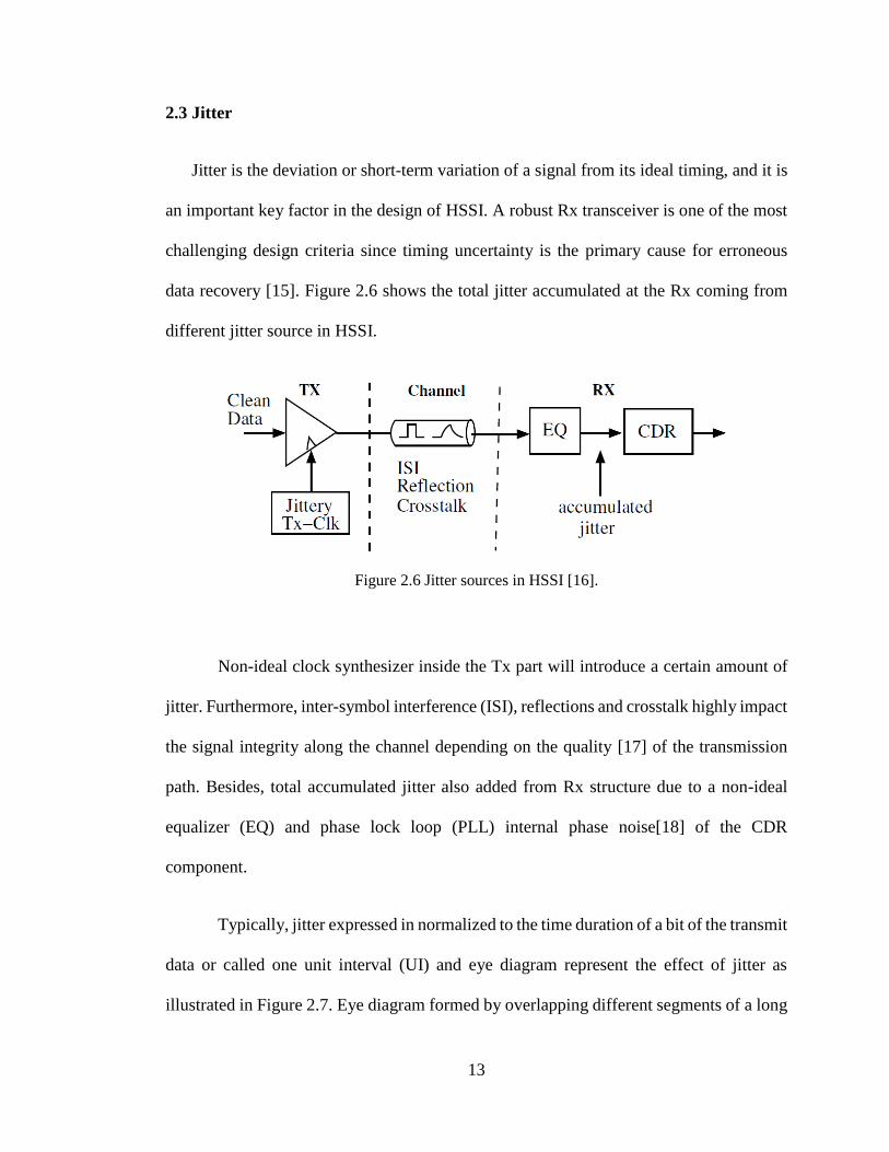
data recovery [15]. Figure 2.6 shows the total jitter accumulated at the Rx coming from
different jitter source in HSSI.
Figure 2.6 Jitter sources in HSSI [16].
Non-ideal clock synthesizer inside the Tx part will introduce a certain amount of
jitter. Furthermore, inter-symbol interference (ISI), reflections and crosstalk highly impact
the signal integrity along the channel depending on the quality [17] of the transmission
path. Besides, total accumulated jitter also added from Rx structure due to a non-ideal
equalizer (EQ) and phase lock loop (PLL) internal phase noise[18] of the CDR
component.
Typically, jitter expressed in normalized to the time duration of a bit of the transmit
data or called one unit interval (UI) and eye diagram represent the effect of jitter as
illustrated in Figure 2.7. Eye diagram formed by overlapping different segments of a long

14
data signal and containing useful information of jitter such as the value of random jitter,
duty cycle distortion (DCD) jitter, inter-symbol interference (ISI), bounded uncorrelated
jitter and periodic jitter.
Figure 2.7 Eye Diagram and its significance [19].
Eye-opening is the main characteristics of an eye diagram that provide useful data
for designers to estimate the system acceptable [20] jitter, and transmission system must
have margin in both the horizontal and vertical eye openings for proper operation.
2.3.1 Classification of jitter
Figure 2.8 shows the classification of jitter components which is the total jitter consists
of a random and deterministic component of jitter. Deterministic jitter composed of
periodic jitter, data dependent jitter and bounded uncorrelated jitter. ISI and DCD are
located under data-dependent jitter.

15
Figure 2.8 Classification of jitter components [22].
Random jitter (RJ) is timing noise that caused by random events and unpredictable
because it has no visible pattern. The main reason is by thermal, flicker and shot noise
[21]. RJ usually quantified by the root mean square (RMS) value and modeled with a
Gaussian probability distribution function (PDF) as shown in Figure 2.9 and can be
calculated by a mean and a standard deviation.
Figure 2.9 Jitter histogram of random jitter [22].

16
Figure 2.10 show the jitter histogram of deterministic jitter. Deterministic jitter is
timing jitter that is repeatable and predictable. Deterministic jitter is further divided into
periodic jitter, data dependent jitter and bounded uncorrelated jitter. This timing jitter is
quantified by bounded peak-to-peak value and normally caused by crosstalk, DCD,
channel losses or spread spectrum clocking.
Figure 2.10 Jitter histogram of deterministic jitter [22].
Periodic jitter or known as sinusoidal jitter is jitter that repeats at a fixed frequency
due to cross coupling from clock or clock drive signal. Data-dependent jitter is associated
with either the transmitted data pattern or aggressor data patterns and divided to ISI and
DCD. ISI is one symbol interfering with another, commonly the previous symbol
influencing the current and caused by limited bandwidth and reflection while DCD is jitter
that is predicted based on whether the associated edge is rising or falling and mainly
caused by offset in Tx threshold and asymmetry in rising and falling edges.

17
Bounded uncorrelated jitter is not aligned in time with the data stream and appears
random. It is most common caused by crosstalk from another signal and classified as
uncorrelated due to being correlated to aggressor signals and not the victim signal or data
stream. While uncorrelated, it is still a bounded source with a quantifiable peak-to-peak
value. Figure 2.11 shows the total jitter PDF produced by convolving the RJ PDF and
deterministic jitter PDF. Both the RMS value of Gaussian component and the peak-to-
peak value of deterministic component separately extracted [23] from the same jitter
histogram to accurately estimate BER.
Figure 2.11 Jitter histogram of total jitter [22].
2.3.2 Jitter tolerance (JTOL)
Jitter tolerance expressed the maximum amplitude of sinusoidal jitter at a specified
frequency that can be tolerated to a receiver while recovering data with specified BER
before it starts to generate errors. A standard jitter tolerance mask is used as a reference
during the test, and the jitter tolerance mask for 12.5 Gb/s Interlaken protocol is shown in
Figure 2.12. This figure indicates that the receiver circuit must be able to track jitter

18
frequencies below 500 kHz with a magnitude up to 5 UI. The unit interval is 80 picosecond
(ps) due to data rate 12.5 Gb/s, and its compliant receiver circuit must be able to track a
data stream at 500 kHz with up to 0.4 nanosecond (ns) of peak-to-peak jitter. Frequencies
higher than 500 kHz, the mask drops by magnitude in discrete steps and at jitter
frequencies greater than 4 MHz, the Rx circuit must tolerate jitter magnitude more than
0.5UI or 40 ps peak-to-peak.
Figure 2.12 Rx JTOL mask for Interlaken protocol [12].
Jitter tolerance test can be performed by encoding the clock into the data stream. The
clock and CDR circuitry assure that the clock and data are in phase when the jitter
frequency is in the bandwidth of the CDR. However, CDR may not track the data, and bit
errors occur if there is high-frequency jitter in the data stream[24]. The objective of jitter
tolerance test is to validate that Rx architecture can operate at a target BER when testing
under worst case conditions.
0.01
0.1
1
10
0.001 0.01 0.1 1 10 100
SJ A
mp
litu
de
(UI)
SJ Frequency (MHz)
Rx JTOL Mask of Interlaken 12.5 Gbps
Mask

19
2.4 Bit error ratio (BER)
Bit error may occur on several occasions in HSSI system, mainly due to the incorrectly
transmitted data stream from Tx component, data distortion along the transmission
channel from one end to another, and incorrect data translation by Rx component.
BER is a basic measurement of the overall channel quality of HSSI system and derived
by calculating the ratio of the total error bits received to the total number of transmitted
bits denoted as,
𝐵𝐸𝑅 =
𝑁𝑒
𝑁𝑇
(2.1)
such that 𝑁𝑒 is the number of bits received in error and 𝑁𝑇 is the total number of bits
transmitted. Jitter and noise shown a significant impact toward BER value when the data
rates are over 3 Gb/s in comparison to lower data rates. Thus, jitter and noise are required
to minimize proportionately at higher data rates in order to sustain an acceptable error
rate.
The conventional method of BER measurement in HSSI system consists of a
pattern generator, a system under test (SUT), and an error detector component as shown
in Figure 2.13. The pattern generator transmits a series of bits known as test pattern into
two component blocks, the SUT, and the error detector. It also supplies a synchronous
clock signal to error detector component to perform a bit-for-bit comparison [25] between
the receiving data from SUT with test pattern data from the pattern generator.

20
Data received from SUT and pattern generator are necessarily needed to be
synchronized to compare accurate bits, whereas dissimilarity between the two sets of data
received by the error detector component deemed as bit error.
The clock signal supplied by pattern generator serves error detector component to
synchronize the test pattern by adapting time delay to the signal hence synchronized the
data received from both ends; the pattern generator and SUT.
Figure 2.13 Equipment setup for BER test [25].
Several factors need to be considered to obtain a reliable BER test result whilst
performing the BER measurement, for instance, a total number of bits need to be
transmitted, and the total number of bit errors need to be captured. Moreover, there is a
minimum requirement value for the BER need to be measure, and it depends on the spec's
definition of the HSSI standard.

21
2.4.1 BER Confidence Level (CL)
The actual required number of transmitted bits depends on the desired BER
confidence level. The BER CL is defined as the probability that the true BER, p(e) is better
than a specified BER level, y or also can define as the percentage of confidence when the
true BER is less than y. Mathematically, CL can be expressed [26] as
𝐶𝐿 = 𝑝 [ 𝑝(𝑒) < 𝑦 | 𝑙, 𝑛 ] (2.2)
where p [ ] indicates a probability, y is a specified BER level, and | l, n denotes a system
where n bits are transmitted, and l bits of errors are detected. Possible values of CL are
range from 0 to 100%.
In term of statistical method involving the binomial distribution function and
Poisson theorem [27], CL denoted as,
𝐶𝐿 = 1 − 𝑒−𝑁 𝑥 𝐵𝐸𝑅𝑠 𝑥 ∑(𝑁 𝑥 𝐵𝐸𝑅𝑠)𝑘
𝑘 !
𝐸
𝑘=0
(2.3)
where 𝑁 is the number of transmitter bits, k is the number of events that took place in N
attempts, 𝐸 is the number of measured bit errors, and 𝐵𝐸𝑅 is the specified bits error rate.
Figure 2.14 shows graph rule of thumb of BER confidence level. This graph can
be used a simple way to calculate the BER CL by multiplying the number of transmitted
bits with the specified BER and draw a horizontal line at this point in the Y-axis. Based
on the appropriate curve the number of detected errors, the CL is where a vertical line
from the curve of the detected errors intersects the X-axis.

22
Figure 2.14 Rule of thumb of BER confidence level [4].
The rule of thumb of BER CL also can be implemented to determine the number
of bits needed to transmit in order to guarantee a specific CL by drawing a vertical line at
the desired CL. From the curve of the estimated number of errors, draw a horizontal line,
and then point where horizontal line intersects the Y-axis is divided by the specified BER
to calculate the required number of transmitted bits.
2.5 JTOL extrapolation
Extrapolation is an estimation or prediction of data based on extending of a known
sequence of data beyond the area that is certainly known [28]. This method can be applied
to estimate the value of jitter for a lower BER based on the jitter measurements from
higher BER values [29]. The significant added advantages of using the extrapolation
method are able to execute fast jitter analysis for lower BER and alleviate measurement
cost. For jitter tolerance extrapolation, the approach of using the Quantile Normalization
of Gaussian tails able to predict the jitter value of lower BER 10-15 based on the measured
data of the higher BER value of 10-11 or 10-12.

23
2.5.1 Mathematical background of Gaussian Quantile Normalization
Jitter tolerance extrapolation developed by mathematical basics of Quantile
Normalization used in linear fitting. The method is inspired by the idea that a quantile-
quantile plot shows a straight diagonal line if the distributions of two data directions are
the same [30] and this concept was extended to multiple samples so that it will have the
same distribution as a result of the normalization procedure.
RJ is assumed to be Gaussian, and if RJ disturbs the signal edge transition, it will
produce Gaussian jitter distribution as shown in Figure 2.15. The probability density
function of Gaussian jitter denoted as,
𝑝 (𝑥) =
1
𝜎√2𝜋 𝑒
−𝑥2
2𝜎2⁄
(2.4)
where 𝜎 is the standard deviation.
Figure 2.15 Probability density function of Gaussian jitter [15].

24
To obtain a standardized representation of the PDF in Equation (2.4), the variable
Q normalizes a Gaussian function with respect to mean, µ and standard deviation, 𝜎 [15]
can be expressed by
𝑄 = 𝑥 − 𝜇
𝜎 (2.5)
Normalized to zero mean and unit variance Q(x) is defined as
𝑄(𝑥) =
1
√2𝜋∫ 𝑒
−𝑥2
2⁄ 𝑑𝑥∞
𝑥
, 𝑥 ≥ 0 (2.6)
The complementary error function is defined as
𝑒𝑟𝑓𝑐 (𝑥) =
2
√𝜋∫ 𝑒−𝑥2
𝑑𝑥∞
𝑥
(2.7)
and hence, Equation (2.6) can be simplified to
𝑄(𝑥) = 1
2 𝑒𝑟𝑓𝑐 (
𝑥
√2) , 𝑥 ≥ 0
(2.8)
The probability density function of the left and right edge transitions of the data
bit as shown in Figure 2.15 can be expressed by
𝑃𝑙𝑒𝑓𝑡(𝑥) =
1
𝜎√2𝜋 𝑒
−𝑥2
2𝜎2⁄
(2.9)
𝑃𝑟𝑖𝑔ℎ𝑡(𝑥) =
1
𝜎√2𝜋 𝑒
−(𝑥−𝑈𝐼)2
2𝜎2⁄
(2.10)