fast algorithms for calculations of viscous …task.gda.pl/files/quart/tq2008/03-04/tq312o-e.pdf ·...
TRANSCRIPT

TASK QUARTERLY 12 No 3, 273–287
FAST ALGORITHMS FOR CALCULATIONS
OF VISCOUS INCOMPRESSIBLE FLOWS
USING THE ARTIFICIAL
COMPRESSIBILITY METHOD
ZBIGNIEW KOSMA
Institute of Applied Mechanics, Technical University of Radom,
Krasickiego 54, 26-600 Radom, Poland
(Received 28 April 2008)
Abstract: An artificial compressibility method is designed to simulate stationary two-and three-
dimensional motions of a viscous incompressible fluid. A standard method of lines approach is
applied in this contribution. A partial differential equation system is discretized in space by second-
order finite-difference schemes on uniform computational grids, and the time-variable is preserved
as continuous. Initial value problems for systems of ordinary differential equations for pressure and
velocity components are computed using the Galerkin-Runge-Kutta method of third order. Some test
calculations for laminar flows in square, cubic, triangular and semicircular cavities with one uniform
moving wall and double bent channels are reported.
Keywords: Navier-Stokes equation, artificial compressibility, method of lines
1. Introduction
One of the early techniques proposed for solving the incompressible Navier-
Stokes equations in a primitive variable form is the artificial compressibility method
of Chorin [1]. In this method, the continuity equation is modified to include an
artificial compressibility term which vanishes when a steady state solution is obtained.
The introduced pseudo-time derivative of pressure directly couples pressure and
velocity and changes the mathematical nature of the continuity equation from elliptic
to hyperbolic. The system of hyperbolic-parabolic equations is well posed and the
efficient numerical methods developed for compressible flows can be used to advance
the system in artificial time.
Many realistic problems in low-speed aerodynamics and hydrodynamics can be
addressed by the incompressible NS equations. In the last two decades, a considerable
progress has been made in developing computational techniques for predicting flow
fields in geometrically complex domains which are of practical interest in engineering
and bioengineering applications. The accuracy and efficiency of the existing codes are
now such that Computational Fluid Dynamics (CFD) is routinely used in the analysis
tq312o-e/273 30IX2008 BOP s.c., http://www.bop.com.pl

274 Z. Kosma
and improvement process of the existing designs and is a valuable tool in experimental
programs and in the construction of new configurations. However, even with the use
of the most powerful super-computers the CPU requirements for steady and unsteady
computations are still very high.
Up to now many efforts have been made in the simulation of viscous flows
by resolving the NS equations with the pseudocompressibility techniques [2–21].
It is usually various highly complicated finite difference schemes that are used for
solving the obtained system of equations, the temporal derivative is approximated via
generalized time differencing. In order to derive a linear algebraic system of equations,
a linearization of viscous and inviscid fluxes has to be performed using Taylor series
expansions.
To overcome the difficulties associated with the nonlinearity of NS equations
a standard method of lines [22–25] approach is applied in this contribution. This
technique offers an advantage over discretized methods in that the NS equations are
linearized. A practical methodology for solving the steady NS equations in arbitrarily
complex geometries is also proposed. Some complex geometrical configurations can
be decomposed into a set of simpler subdomains. Each of them is designed to be
easily discretized with a simple rectangular grid. The simplest approach for specifying
boundary conditions near a curved or irregular boundary is to transfer all primitive
variables from the boundary to the nearest grid knots. In this way the system of
partial differential equation is discretized in space by second-order finite-difference
schemes on uniform grids in physical domains with the same mesh sizes in each
direction, to be then integrated in time. The initial-boundary value problem for the
system of partial differential equations is then reduced to an initial value problem
for the system of ordinary differential equations (mathematically parabolic) which
can be solved numerically by any powerful ordinary differential equations solver.
To simplify our analysis, this study focuses only on the frequently studied standard
benchmark problems to validate the accuracy of the NS solvers because many approved
experimental and numerical results have been reported in the literature.
2. Governing equations
With the pseudo-compressibility technique the non-dimensionalized governing
equations in the Cartesian co-ordinate system become:
∂p
∂t+1
β
∂Vj∂xj=0,
∂Vi∂t+∂
∂xjViVj =−
∂p
∂xi+1
Re
∂
∂xj
∂
∂xjVi,
(1)
where V1, V2, V3 are the velocity components, p is the pressure, Re is the Reynolds
number, and β > 0 is the artificial compressibility parameter.
In the first component of the above equations, a time derivative of pressure is
artificially added to the equation of continuity. However, since mass conservation is
enforced only at the steady state, it is impossible to follow a physical time transient.
The artificial compressibility factor β represents an artificial sound speed and
affects the overall convergence rate. It is possible to increase the rate of convergence
by selecting an optimum value of β, but this has to be done on a trial and error basis
tq312o-e/274 30IX2008 BOP s.c., http://www.bop.com.pl

Fast Algorithms for Calculations of Viscous Incompressible Flows. . . 275
for each problem. Through several computational experiments, the most convenient
value of the pseudo-compressibility parameter β has been found to be unity and this
value will be kept constant in the entire domains of solution.
The physical boundary conditions for the equations of viscous flows (1) in
primitive variables are specified as consisting of impermeability as well as of non-
slip conditions at solid walls and of the requirement of assumed velocity profiles at
channel inlets and outlets. The pressure is usually not given on the boundaries, but
it can be determined from the momentum equations, and can be fixed in one point
of the domain.
The original form of the artificial compressibility method has been developed
for the steady-state problems [3, 5]. The first of equations (1) can be used to compute
pressure fields. The method can also be extended to a time accurate formulation and
there are numerous works in the literature describing various strategies for solving
the unsteady flow problems, see e.g. [10, 13–16]. The time accurate solutions can be
obtained by using a three-level formula to evaluate the time derivatives and adding
a pseudo time-derivative in the momentum equations. The discretized momentum
equations are solved for a divergence free velocity field at each successive time level.
3. Numerical approach
The proposed numerical technique, the method of lines, consists of converting
the partial differential equations system (1) into an ordinary differential equation ini-
tial value problem by discretizing the spatial derivatives together with the boundary
conditions for the first derivative of pressure via the classical finite difference approxi-
mations of second order [26]. This produces a system of ordinary differential equations
of the general form:dU
dt=F (U ), (2)
where U = [p,Vi]T is the vector of dependent variables, and F is a spatial differential
operator.
The unknown values of pressure and velocity components in each inner knot of
computational meshes are computed using the explicit Galerkin-Runge-Kutta method
of third order [27]:
U (1)=Un+∆tF (Un),
U (2)=3
4Un+
1
4U (1)+
1
4∆tF (U (1)),
Un+1=1
3Un+
2
3U (2)+
2
3∆tF (U (2)).
(3)
Time advancement to a steady-state of viscous flows obtained with the third-
order explicit Runge-Kutta-Galerkin method proved to be much more efficient than
the backward-differentiation predictor-corrector method [28, 29].
4. Numerical simulation of various fluid flows
Numerical methods for incompressible Navier-Stokes equations are often verified
for codes validation, on widely used benchmark problems; the driven square [30–55]
and cubic cavity flows [38, 56–67]. The streamlines and comparisons between the
results of the method of lines and those found in the literature are shown. Some other
tq312o-e/275 30IX2008 BOP s.c., http://www.bop.com.pl
276 Z. Kosma
numerical experiments with incompressible fluid flows are also considered: double bent
channel flows as well as triangular and semi-circular driven cavity flows.
4.1. Square and cubic cavity problems
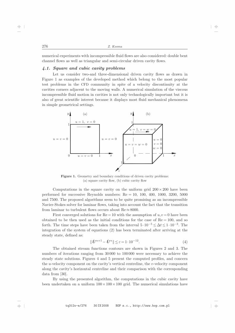
Let us consider two-and three-dimensional driven cavity flows as drawn in
Figure 1 as examples of the developed method which belong to the most popular
test problems in the CFD community in spite of a velocity discontinuity at the
cavities corners adjacent to the moving walls. A numerical simulation of the viscous
incompressible fluid motion in cavities is not only technologically important but it is
also of great scientific interest because it displays most fluid mechanical phenomena
in simple geometrical settings.
Figure 1. Geometry and boundary conditions of driven cavity problems:
(a) square cavity flow, (b) cubic cavity flow
Computations in the square cavity on the uniform grid 200×200 have been
performed for successive Reynolds numbers: Re = 10, 100, 400, 1000, 3200, 5000
and 7500. The proposed algorithms seem to be quite promising as an incompressible
Navier-Stokes solver for laminar flows, taking into account the fact that the transition
from laminar to turbulent flows occurs about Re≈ 8000.
First converged solutions for Re=10 with the assumption of u,v=0 have been
obtained to be then used as the initial conditions for the case of Re = 100, and so
forth. The time steps have been taken from the interval 5 ·10−5 ≤∆t≤ 1 ·10−3. The
integration of the system of equations (2) has been terminated after arriving at the
steady state, defined as:
‖U n+1−U n‖≤ ε=1 ·10−12. (4)
The obtained stream functions contours are shown in Figures 2 and 3. The
numbers of iterations ranging from 30000 to 100000 were necessary to achieve the
steady state solutions. Figures 4 and 5 present the computed profiles, and concern
the u-velocity component on the cavity’s vertical centreline, the v-velocity component
along the cavity’s horizontal centreline and their comparison with the corresponding
data from [30].
By using the presented algorithm, the computations in the cubic cavity have
been undertaken on a uniform 100×100×100 grid. The numerical simulations have
tq312o-e/276 30IX2008 BOP s.c., http://www.bop.com.pl

Fast Algorithms for Calculations of Viscous Incompressible Flows. . . 277
Figure 2. Square cavity: stream-function contours for
Re=1000 (left) and 3200 (right), 200×200 grid
Figure 3. Square cavity: stream-function contours for
Re=5000 (left) and 7500 (right), 200×200 grid
Figure 4. Distributions of x- and y-components of velocity on 2D-cavity centrelines
at Re=5000, 200×200 grid; solid line – the presented method, triangles – Ghia et al.,
x=0.5 (left), y=0.5 (right)
been conducted with ∆t=1 ·10−3 for the Reynolds numbers: Re= 10, 100, 400 and
1000. The solutions have been qualified as steady for the relative error (4) between
two time steps. It takes approximately 50000–80000 time steps to converge. The
tq312o-e/277 30IX2008 BOP s.c., http://www.bop.com.pl
278 Z. Kosma
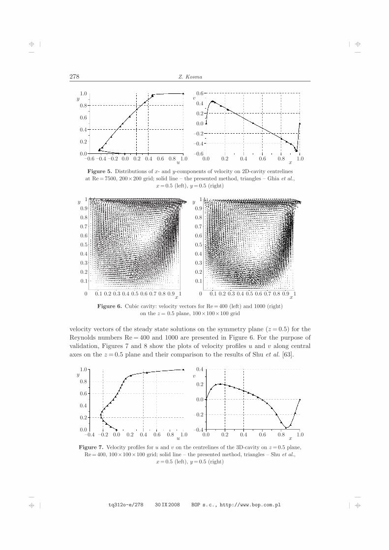
Figure 5. Distributions of x- and y-components of velocity on 2D-cavity centrelines
at Re=7500, 200×200 grid; solid line – the presented method, triangles – Ghia et al.,
x=0.5 (left), y=0.5 (right)
Figure 6. Cubic cavity: velocity vectors for Re=400 (left) and 1000 (right)
on the z= 0.5 plane, 100×100×100 grid
velocity vectors of the steady state solutions on the symmetry plane (z=0.5) for the
Reynolds numbers Re= 400 and 1000 are presented in Figure 6. For the purpose of
validation, Figures 7 and 8 show the plots of velocity profiles u and v along central
axes on the z=0.5 plane and their comparison to the results of Shu et al. [63].
Figure 7. Velocity profiles for u and v on the centrelines of the 3D-cavity on z=0.5 plane,
Re=400, 100×100×100 grid; solid line – the presented method, triangles – Shu et al.,
x=0.5 (left), y=0.5 (right)
tq312o-e/278 30IX2008 BOP s.c., http://www.bop.com.pl

Fast Algorithms for Calculations of Viscous Incompressible Flows. . . 279
Figure 8. Velocity profiles for u and v on 3D-cavity centrelines on z=0.5 plane,
Re=1000, 100×100× 100 grid; solid line – the presented method, triangles – Shu et al.,
x=0.5 (left), y=0.5 (right)
4.2. Flow in double bent channels
The aim of this test case [47, 68–70] is to demonstrate the effectiveness of
the presented numerical algorithms and artificial compressibility formulation of the
Navier-Stokes equations in geometrical domains bounded by contours consisting of
finite numbers of rectilinear segments, parallel to the axes of the co-ordinate system.
An example of the flow in double bent channels with two concave corners is considered.
Figure 9 shows the geometry in which all the channels have the height of H =1, the
upper and lower channels lengths have been maintained in all configurations by setting
L1=2 and L3=9 with the channel step ratio of H ≤L2≤ 5H.
A parabolic velocity profile is imposed as the boundary conditions at the upper
channel inlet and a zero pressure gradient is assumed. The non-slip condition on the
solid walls is prescribed for the velocity components and the pressure is computed with
the known normal pressure gradients from the Navier-Stokes equations. The outlet
velocity field in the lower channel is also specified as a parallel flow with a parabolic
velocity profile and the pressure is set as equal to a constant value.
Figure 9. Geometry for double bent channels
tq312o-e/279 30IX2008 BOP s.c., http://www.bop.com.pl

280 Z. Kosma
The applied methodology consists in decomposition of the computational
domain into a set of rectangles. After the domain decomposition has been completed,
the relative location of the various rectangles and the manner in which they are
connected with each other need to be determined, the sets of rectangular co-
ordinates determine every rectangle separately. The solution to this problem, which
is collectively referred to as grid connectivity, is trivial even when a large number of
adjacent rectangles is employed.
Figure 10. Schematic of a double bent channel domain with three adjacent rectangles
Using the developed algorithm, calculations for double bent channels flows
have been performed for Re ≤ 200 on two (L2 = 1): 100× 50, 50L× 50 or three
(L2 > 1): 100× 50, 50× 50L and 50L× 50 uniform grids (Figure 10) for channels
lengths 1 ≤ L ≤ 9. The original problem is solved on each successive rectangle for
the known tentative values of velocity components and pressure separately, and the
values on the adjacent boundaries are exchanged. The calculations have been made
with ∆t=1 ·10−3 and 10000–90000 time steps on each grid have been necessary to
get convergent solutions. Figures 11–13 show the computed stream-function contours
for three channel step ratios L2=1,3,5, respectively.
Figure 11. Double bent channel: stream-function contours, Re=200, L2=1
Figure 12. Double bent channel: stream-function contours, Re=200, L2=3
tq312o-e/280 30IX2008 BOP s.c., http://www.bop.com.pl
Fast Algorithms for Calculations of Viscous Incompressible Flows. . . 281
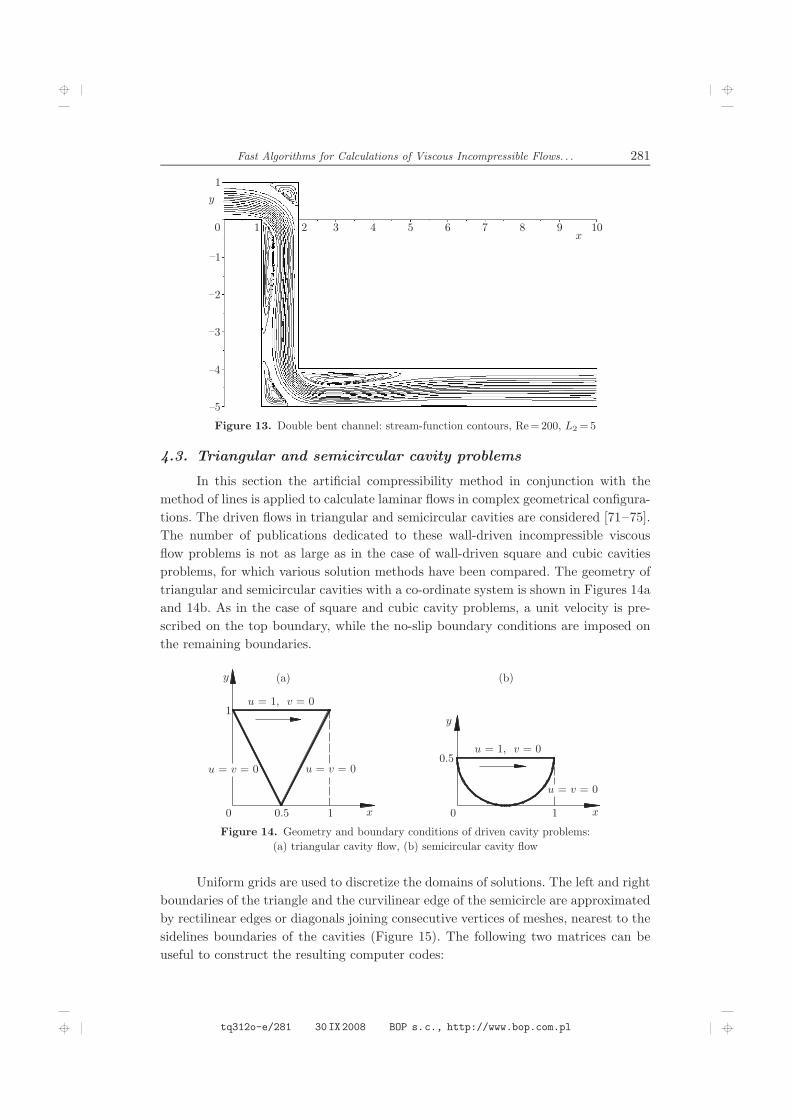
Figure 13. Double bent channel: stream-function contours, Re=200, L2=5
4.3. Triangular and semicircular cavity problems
In this section the artificial compressibility method in conjunction with the
method of lines is applied to calculate laminar flows in complex geometrical configura-
tions. The driven flows in triangular and semicircular cavities are considered [71–75].
The number of publications dedicated to these wall-driven incompressible viscous
flow problems is not as large as in the case of wall-driven square and cubic cavities
problems, for which various solution methods have been compared. The geometry of
triangular and semicircular cavities with a co-ordinate system is shown in Figures 14a
and 14b. As in the case of square and cubic cavity problems, a unit velocity is pre-
scribed on the top boundary, while the no-slip boundary conditions are imposed on
the remaining boundaries.
Figure 14. Geometry and boundary conditions of driven cavity problems:
(a) triangular cavity flow, (b) semicircular cavity flow
Uniform grids are used to discretize the domains of solutions. The left and right
boundaries of the triangle and the curvilinear edge of the semicircle are approximated
by rectilinear edges or diagonals joining consecutive vertices of meshes, nearest to the
sidelines boundaries of the cavities (Figure 15). The following two matrices can be
useful to construct the resulting computer codes:
tq312o-e/281 30IX2008 BOP s.c., http://www.bop.com.pl

282 Z. Kosma
– a two-dimensional matrix with logical elements to the identification mesh knots
which determine step-shaped lines approximating the unmoving boundaries of
the cavities,
– a one-dimensional matrix with integer elements containing numbers of the first
inner knots on vertical grid lines.
The systems of semi-discrete (discrete in space, continuous in time) ordinary
differential equations (2) can be thus obtained in all the nodes of the assumed uniform
computational grids situated inside the boundaries of cavities.
Figure 15. Some curved boundary line approximations
The flow in the triangular cavity has been simulated for Reynolds numbers
of Re≤ 5000 with the mesh size h= 1/300, the flow in the semicircular cavity – for
Reynolds numbers of Re≤ 6600 with the mesh size h=1/250. The computations have
been done with the time step ∆t=1 ·10−4 until the criterion (4) for convergence has
been satisfied. The obtained velocity vectors and stream function contours for some
Reynolds numbers are presented in Figures 16–22.
5. Remarks and conclusions
A very efficient and accurate numerical approach based on the artificial com-
pressibility and lines methods is developed in this work for predicting steady laminar
flows at high Reynolds numbers. The time integration has been obtained by the
third-stage Galerkin-Runge-Kutta scheme. The details of the numerical procedure
employed to solve the governing equations are presented, and a brief description of
the applied strategy is provided. The proposed algorithms have proved to be very ef-
fective for the demanded time of calculations required for steady-state computations,
they offer a significant acceleration of computations in comparison with the previous
algorithms [28, 29], and the calculation time of the same problem solutions obtained
by using the Fluent solver.
Simulations of 2D and 3D lid-driven cavity flows as well as flows in double bent
channels and triangular and semicircular cavities have been performed for various
Reynolds numbers. The steady-state numerical results for these flows are compared
to the results reported in the literature. It has been found that the proposed approach
yields the same velocity profiles along the vertical and horizontal lines on the mid-
plane of square and cubic cavities and the same velocity and stream-function fields in
the other regarded domains.
In the past decades, much progress has been made in developing computational
techniques for predicting flow fields in complex geometries. The widely used methods
have included finite element and finite volume methods due to their ability to analyze
the domains of an arbitrary shape. Although automatic grid generation is usually
a very effective solution, the mesh is difficult to be fully generated in many engineering
tq312o-e/282 30IX2008 BOP s.c., http://www.bop.com.pl

Fast Algorithms for Calculations of Viscous Incompressible Flows. . . 283
Figure 16. Triangular cavity: velocity vectors and stream-function contours for
Re=1000, mesh size h=1/300
Figure 17. Triangular cavity: velocity vectors and stream-function contours for
Re=3000, mesh size h=1/300
Figure 18. Triangular cavity: velocity vectors and stream-function contours for
Re=5000, mesh size h=1/300
tq312o-e/283 30IX2008 BOP s.c., http://www.bop.com.pl

284 Z. Kosma
Figure 19. Semicircular cavity: velocity vectors and stream-function contours for
Re=1000, mesh size h=1/250
Figure 20. Semicircular cavity: velocity vectors and stream-function contours for
Re=2000, mesh size h=1/250
Figure 21. Semicircular cavity: velocity vectors and stream-function contours for
Re=4000, mesh size h=1/250
Figure 22. Semicircular cavity: velocity vectors and stream-function contours for
Re=6600, mesh size h=1/250
problems, and pre-specified connectivity between the computational nodes or grid
points is required. In order to avoid the troublesome processing of mesh generation,
a number of meshless methods have been proposed in which the analysis domain
is discretized without employing any mesh or elements. Mesh-free methods usually
require node generation instead of mesh generation. Functions and their derivatives at
one central node are approximated entirely from the information of a set of scattered
tq312o-e/284 30IX2008 BOP s.c., http://www.bop.com.pl

Fast Algorithms for Calculations of Viscous Incompressible Flows. . . 285
nodes within its local support. From the point of view of computational efforts, node
generation is considered to be an easier and faster job, compared to the former one.
Rather than calling these methods an alternative for meshbased methods, they may
be labeled as specific tools because the price to pay is a relatively high computational
burden associated with the use of these methods.
An alternative and practical methodology for solving the Navier-Stokes equa-
tions in arbitrarily complex geometries using Cartesian meshes which have numerous
inherent advantages is proposed in the paper. These include simple and efficient field
mesh generation, superior implementation of discretization schemes, minimal asso-
ciated phase errors, and absence of any issues associated with mesh skewness and
distortion. However, an obvious difficulty with the Cartesian approach is the imple-
mentation of solid wall boundary conditions, and their approximation error strongly
depends on the mesh size value. The scheme presented in this paper is spatially
isotropic (which is important for general applications) and shows good stability and
accuracy in the test problems solved. The schemes have been presented and tested for
two-dimensional solutions, but in principle the given procedure can also be developed
directly for three-dimensional analyses. Of course, further studies of the scheme, for
two-dimensional solutions are needed to include the numerical effectiveness. The po-
tential of the domain decomposition method onto a set of rectangles with rectilinear
or curved sides is demonstrated as a technique for simulating complex engineering
flows. Besides, near curved or irregular boundaries unequal mesh spacings and spe-
cial rules may be considered. The research in this direction is in progress. Because
the tentative velocity and pressure fields are given, the numerical calculations in each
subdomain can be done separately. The extension of the algorithms provides a tool for
studying problems in many engineering applications that involve complex geometries
and flows.
References
[1] Chorin A J 1967 J. Comput. Phys. 2 12
[2] Liu H and Ikehata M 1994 Int. J. Numer. Meth. Fluids 19 395
[3] Pentaris A, Nikolados K and Tsangaris S 1994 Int. J. Numer. Meth. Fluids 19 1013
[4] Anderson W K, Rausch R D and Bonhaus D L 1996 J. Comput. Phys. 128 391
[5] Pappou T and Tsangaris S 1997 Int. J. Numer. Meth. Fluids 25 523
[6] Liu C, Zheng X and Sung C H 1998 J. Comput. Phys. 139 35
[7] Dridakis D, Iliev O P and Vassileva D P 1998 J. Comput. Phys. 146 301
[8] Yuan L 2002 J. Comput. Phys. 177 134
[9] He X, Doolen G D and Clark T 2002 J. Comput. Phys. 179 439
[10] Tang H S, Jones S C and Sotiropoulos F 2003 J. Comput. Phys. 191 567
[11] Tai C H and Zhao Y 2003 J. Comput. Phys. 192 277
[12] Mendez B and Velazquez A 2004 Comput. Meth. Appl. Mech. Engrg. 193 825
[13] Ekaterinaris J A 2004 Int. J. Numer. Meth. Fluids 45 1187
[14] Kallinderis Y and Ahn H T 2005 J. Comput. Phys. 210 75
[15] Shapiro E and Drikakis D 2005 J. Comput. Phys. 210 584
[16] Shapiro E and Drikakis D 2005 J. Comput. Phys. 210 608
[17] Nithiarasu P and Liu C-B 2006 Comput. Meth. Appl. Mech. Engrg. 195 2961
[18] Lin P T, Baker T J, Martinelli L and Jameson A 2006 Int. J. Numer. Meth. Fluids 50 199
[19] Lee J W, Teubner M D, Nixon J B and Gill P M 2006 Int. J. Numer. Meth. Fluids 51 617
[20] Nithiarasu P and Zienkiewicz O C 2006 Comput. Meth. Appl. Mech. Engrg. 195 5537
[21] Tang H S and Sotiropoulus F 2007 Comput. Fluids 36 974
tq312o-e/285 30IX2008 BOP s.c., http://www.bop.com.pl
286 Z. Kosma
[22] Oymak O and Selcuk N 1996 Int. J. Numer. Meth. Fluids 23 455
[23] Solin P and Segeth K 2003 Int. J. Numer. Meth. Fluids 41 519
[24] Tang H and Warnecke G 2005 Comput. Fluids 34 375
[25] 2005 J. Comput. Appl. Math. 183 241 (Special Issue on the Method of Lines)
[26] Kosma Z 2008 Numerical Methods for Engineering Applications, 5 th Edition, Technical
University of Radom Publishing (in Polish)
[27] Cockburn B and Shu C-W 1998 J. Comput. Phys. 141 199
[28] Kosma Z and Noga B 2006 Chemical Process Engrg. 27 761
[29] Kosma Z 2007 Numerical simulation of viscous fluid motions using the artificial compress-
ibility method, Monography of Technical University of Radom (in Polish)
[30] Ghia U, Ghia K N and Shin C T 1982 J. Comput. Phys. 48 387
[31] Kim J and Moin P 1985 J. Comput. Phys. 59 308
[32] Tanahashi T and Okanaga H 1990 Int. J. Numer. Meth. Fluids 11 479
[33] Kovacs A and Kawahara M 1991 Int. J. Numer. Meth. Fluids 13 403
[34] Ren G and Utnes T 1993 Int. J. Numer. Meth. Fluids 17 349
[35] Li M, Tang T and Fornberg B 1995 Int. J. Numer. Meth. Fluids 20 1137
[36] Barragy E and Carey G F 1997 Comput. Fluids 26 453
[37] Botella O and Peyret R 1998 Comput. Fluids 27 421
[38] Shankar P N and Deshpande M D 2000 Annu. Rev. Fluid Mech. 32 93
[39] Aydin M and Fenner R T 2001 Int. J. Numer. Meth. Fluids 37 45
[40] Barton I E, Markham-Smith D and Bressloff N 2002 Int. J. Numer. Meth. Fluids 38 747
[41] Peng Y-F, Shiau Y-H and Hwang R R 2003 Comput. Fluids 32 337
[42] Mai-Duy N and Tran-Cong T 2003 Int. J. Numer. Meth. Fluids 41 743
[43] Sahin M and Owens R G 2003 Int. J. Numer. Meth. Fluids 42 57
[44] Sahin M and Owens R G 2003 Int. J. Numer. Meth. Fluids 42 79
[45] Piller M and Stalio E 2004 J. Comput. Phys. 197 299
[46] Gravemeier V, Wall W A and Ramm E 2004 Comput. Meth. Appl. Mech. Engrg. 193 1323
[47] Ramsak M and Skerget L 2004 Int. J. Numer. Meth. Fluids 46 815
[48] Wu Y and Liao S 2005 Int. J. Numer. Meth. Fluids 47 185
[49] Erturk E, Corke T C and Gokcol C 2005 Int. J. Numer. Meth. Fluids 48 747
[50] Bruger A, Gustafsson B, Lotstedt P and Nilsson J 2005 J. Comput. Phys. 203 49
[51] Abide S and Viazzo S 2005 J. Comput. Phys. 206 252
[52] Gelhard T, Lube G, Olshanskii M A and Starcke J-H S 2005 J. Comput. Appl. Math. 177 243
[53] Bruneau C-H and Saad M 2006 Comput. Fluids 35 326
[54] Masud A and Khurram R A 2006 Comput. Meth. Appl. Mech. Engrg. 195 1750
[55] Prabhakar V and Reddy J N 2006 J. Comput. Phys. 215 274
[56] Guy G and Stella F 1993 J. Comput. Phys. 106 286
[57] Jiang B-N, Lin T L and Povinelli L A 1994 Comput. Meth. Appl. Mech. Engrg. 114 213
[58] Tang L Q, Cheng T and Tsang T T H 1995 Int. J. Numer. Meth. Fluids 21 413
[59] Dridakis D, Iliev O P and Vassileva D P 1998 J. Comput. Phys. 146 301
[60] Paisley M F 1999 Int. J. Numer. Meth. Fluids 30 441
[61] Liu C H 2001 Int. J. Numer. Meth. Fluids 35 533
[62] Sheu T W H and Tsai S F 2002 Comput. Fluids 31 911
[63] Shu C, Wang L and Chew Y T 2003 Int. J. Numer. Meth. Fluids 43 345
[64] Nithiarasu P, Mathur J S, Weatherill N P and Morgan K 2004 Int. J. Numer. Meth. Fluids
44 1207
[65] Lo D C, Murugesan K and Young D L 2005 Int. J. Numer. Meth. Fluids 47 1469
[66] Albensoeder S and Kuhlmann H C 2005 J. Comput. Phys. 206 536
[67] Ding H, Shu C, Yeo K S and Xu D 2006 Comput. Meth. Appl. Mech. Engrg. 195 516
[68] Tulapurkara E G, Lakshmana Gowda B H and Balachandran N 1988 J. Fluid Mech. 190 179
[69] Hwang Y-H 1994 J. Comput. Phys. 110 134
[70] Bathe K-J and Zhang H 2002 J. Comput. Phys. 80 1267
[71] Jyotsna R and Vanka S P 1995 J. Comput. Phys. 122 107
tq312o-e/286 30IX2008 BOP s.c., http://www.bop.com.pl
Fast Algorithms for Calculations of Viscous Incompressible Flows. . . 287
[72] Lai M-J and Wenston P 2004 Comput. Fluids 33 1047
[73] Kohno H and Bathe K-J 2006 Int. J. Numer. Meth. Fluids 51 673
[74] Glowinski R, Guidoboni G and Pan T-W 2006 J. Comput. Phys. 216 76
[75] Pontaza J P 2007 J. Comput. Phys. 221 649
tq312o-e/287 30IX2008 BOP s.c., http://www.bop.com.pl
288 TASK QUARTERLY 12 No 3
tq312o-e/288 30IX2008 BOP s.c., http://www.bop.com.pl