Fast Adaptive Digital Pre-Distortion Scheme for

Application in Cellular Base Station Power

Amplifiers

by

Francisca Funmilayo Adaramola, B.Eng.

A thesis submitted to the

Faculty of Graduate and Postdoctoral Affairs

in partial fulfillment of the requirements for the degree of

Master of Applied Science in Electrical Engineering

Ottawa-Carleton Institute for Electrical and Computer Engineering

Department of Systems and Computer Engineering

Carleton University

Ottawa, Ontario

June, 2015

c©Copyright

Francisca Funmilayo Adaramola, 2015

The undersigned hereby recommends to the

Faculty of Graduate and Postdoctoral Affairs

acceptance of the thesis

Fast Adaptive Digital Pre-Distortion Scheme for Application

in Cellular Base Station Power Amplifiers

submitted by Francisca Funmilayo Adaramola, B.Eng.

in partial fulfillment of the requirements for the degree of

Master of Applied Science in Electrical Engineering

Professor Howard Schwartz, Thesis Co-supervisor

Professor Thomas Kunz, Thesis Co-supervisor

Professor Roshdy Hafez, Chair,Department of Systems and Computer Engineering

Ottawa-Carleton Institute for Electrical and Computer Engineering

Department of Systems and Computer Engineering

Carleton University

June, 2015

ii

Abstract

In a base station, the power amplifier (PA) experiences rapid fluctuations in behavior

because of the varying power levels and bandwidth of its excitation signals. High

peak-to-average power ratios and non-constant envelopes of wideband signals impose

stringent linear and efficiency requirements on the PA required for amplification.

It is necessary to design fast and non-complex digital pre-distorters that are able

to achieve and maintain acceptable linearization performance and compensate for

the dynamic distortions generated by the PA. This thesis explores an adaptive DPD

scheme using multiple model control that combines a switching and a simple adapta-

tion algorithm.

Experimental data are used in evaluating the proposed scheme. The multiple

model scheme reduces the transient error response and requires a relatively small

number of data samples for identification, switching and adaptation. The scheme is

demonstrated to be fast, less complex, and capable of maintaining and achieving the

linearity requirement of the PA.

iii

Acknowledgments

All thanks to God Almighty for the opportunity, ability and grace to begin and

complete this research work. Only by Him, through Him and for Him was this work

possible.

Sincere thanks to my supervisors: Howard Schwartz and Thomas Kunz, for be-

lieving in me, guiding and leading me patiently and constantly to the completion of

this thesis. Thanks to Mark Wyville for the effort, technical support and contribution

and to Ericsson for their support that has made this thesis possible.

Gratefully acknowledge the help and support received from staff, professors,

friends and colleagues I have met during the period of my study. Appreciation goes

to Tosin Olopade and Abubakar Hasssan for your assistance and help in answering

all my questions. Thanks to the PhD students in Research Lab 7070 for the fruitful

discussions directions and interactions during the work.

Finally, thank you to my family for their encouragement, love and support in all

my endeavours.

iv

Table of Contents

Abstract iii

Acknowledgments iv

Table of Contents v

List of Tables ix

List of Figures xi

Nomenclature xvi

1 Introduction 1

1.1 Overview . . . . . . . . . . . . . . . . . . . . . . . . . . . . . . . . . . 1

1.2 Thesis / Problem Statement . . . . . . . . . . . . . . . . . . . . . . . 5

1.3 Objectives/ Motivation . . . . . . . . . . . . . . . . . . . . . . . . . . 6

1.4 Contributions . . . . . . . . . . . . . . . . . . . . . . . . . . . . . . . 6

1.5 Organization of the Thesis . . . . . . . . . . . . . . . . . . . . . . . . 7

2 Background on Power Amplifier 8

2.1 Introduction . . . . . . . . . . . . . . . . . . . . . . . . . . . . . . . . 8

2.2 PA Nonlinearity and Memory Effect . . . . . . . . . . . . . . . . . . . 8

2.3 Power Amplifier Characterization . . . . . . . . . . . . . . . . . . . . 11

v

2.3.1 Amplitude and Phase Distortions . . . . . . . . . . . . . . . . 14

2.3.2 Adjacent Channel Power Ratio . . . . . . . . . . . . . . . . . 15

2.3.3 Normalised Mean Square Error . . . . . . . . . . . . . . . . . 16

2.4 PA Modeling . . . . . . . . . . . . . . . . . . . . . . . . . . . . . . . 17

2.4.1 Memoryless Nonlinear Models . . . . . . . . . . . . . . . . . . 18

2.4.2 Memory Nonlinear Models . . . . . . . . . . . . . . . . . . . . 19

3 Adaptive Digital Pre-distortion 24

3.1 Introduction . . . . . . . . . . . . . . . . . . . . . . . . . . . . . . . . 24

3.2 Pre-distortion . . . . . . . . . . . . . . . . . . . . . . . . . . . . . . . 25

3.3 Inverse Modeling . . . . . . . . . . . . . . . . . . . . . . . . . . . . . 28

3.4 Memory Model Based Digital Pre-distortion Schemes . . . . . . . . . 30

3.5 Model Parameters Identification and Estimation Algorithms . . . . . 33

3.5.1 Least Squares Algorithm . . . . . . . . . . . . . . . . . . . . . 34

3.5.2 Adaptive Algorithms . . . . . . . . . . . . . . . . . . . . . . . 35

3.6 Review of Adaptive Digital Pre-distortion Schemes . . . . . . . . . . 38

3.7 Improvement to Adaptive DPD Schemes . . . . . . . . . . . . . . . . 39

4 Multiple Model Baseband Adaptive Digital Pre-distortion 41

4.1 Introduction . . . . . . . . . . . . . . . . . . . . . . . . . . . . . . . . 41

4.2 Data Signals Structure . . . . . . . . . . . . . . . . . . . . . . . . . . 41

4.3 Characterization of the PA . . . . . . . . . . . . . . . . . . . . . . . . 43

4.4 Time Delay Estimation and Alignment . . . . . . . . . . . . . . . . . 44

4.5 Scaling of Output Data . . . . . . . . . . . . . . . . . . . . . . . . . . 44

4.6 Data Pre-processing . . . . . . . . . . . . . . . . . . . . . . . . . . . 45

4.7 Static Digital Pre-distortion Synthesis . . . . . . . . . . . . . . . . . . 46

4.8 Adaptive Digital Pre-distortion Synthesis . . . . . . . . . . . . . . . . 49

vi

4.9 Multiple Model Digital Pre-distortion . . . . . . . . . . . . . . . . . . 51

4.9.1 Offline Parameterization for Model Placement . . . . . . . . . 53

4.9.2 Hypothesis Test Switching Algorithm . . . . . . . . . . . . . . 56

4.9.3 Selected Model Adaptation . . . . . . . . . . . . . . . . . . . . 59

4.10 Multiple Model Configuration . . . . . . . . . . . . . . . . . . . . . . 61

4.11 Scheme Evaluation . . . . . . . . . . . . . . . . . . . . . . . . . . . . 62

4.11.1 Linearization Performance . . . . . . . . . . . . . . . . . . . . 62

4.11.2 Complexity and Speed . . . . . . . . . . . . . . . . . . . . . . 64

5 Simulation Results 66

5.1 Testbed Equipment Platform Setup . . . . . . . . . . . . . . . . . . . 66

5.2 Data Measurement Procedure . . . . . . . . . . . . . . . . . . . . . . 68

5.3 Time Alignment Results . . . . . . . . . . . . . . . . . . . . . . . . . 73

5.4 PA Characterization . . . . . . . . . . . . . . . . . . . . . . . . . . . 74

5.5 Static DPD Simulation . . . . . . . . . . . . . . . . . . . . . . . . . . 76

5.5.1 PA and DPD Modeling Simulation . . . . . . . . . . . . . . . 77

5.5.2 Static DPD Linearization Performance . . . . . . . . . . . . . 80

5.5.3 Effect of Power Levels, Bandwidth and Model Configuration on

Linearization Performance . . . . . . . . . . . . . . . . . . . . 83

5.6 First Order Linear Digital Pre-distortion . . . . . . . . . . . . . . . . 86

5.7 Memory Polynomial Based Adaptive DPD Simulation . . . . . . . . . 90

5.8 Multiple Model Switching Algorithm . . . . . . . . . . . . . . . . . . 94

5.9 Uniform Configuration Multiple Model Performance . . . . . . . . . . 95

5.10 Discussion . . . . . . . . . . . . . . . . . . . . . . . . . . . . . . . . . 99

5.11 Non-uniform Configuration Multiple Model Performance . . . . . . . 103

5.12 Discussion . . . . . . . . . . . . . . . . . . . . . . . . . . . . . . . . . 107

vii

5.13 Online Adaptive Parameter Learning . . . . . . . . . . . . . . . . . . 107

5.14 Number of Models Reduction . . . . . . . . . . . . . . . . . . . . . . 109

5.15 Summary . . . . . . . . . . . . . . . . . . . . . . . . . . . . . . . . . 109

6 Conclusion and Future Work 111

6.1 Conclusion . . . . . . . . . . . . . . . . . . . . . . . . . . . . . . . . . 111

6.2 Future Work . . . . . . . . . . . . . . . . . . . . . . . . . . . . . . . . 113

List of References 115

viii

List of Tables

4.1 Possible PA and DPD model structure and configuration choice . . . 47

5.1 List of measured input and output multicarrier signals at different ith

power levels. The label i is the index of the input signal’s power level

that specifies the ith operating condition. The label (Di) represents the

index of the dataset (input and corresponding output) with a carrier

size and at a specific ith power level setting . . . . . . . . . . . . . . 71

5.2 ACPR values of measured datasets for simulation . . . . . . . . . . . 76

5.3 Modeling accuracy results from the PA and DPD modeling for different

configurations using 2C-WCDMA and 4C-WCDMA at the same power

level. The number of parameters estimated from each configuration is

represented as KM . . . . . . . . . . . . . . . . . . . . . . . . . . . . 78

5.4 Comparison of the PA and DPD modeling accuracy with a fixed con-

figuration for the 2C-WCDMA signal at different power levels . . . . 80

5.5 Comparison of the ACPR and NMSE of the PA output with a DPD

modeled with datasets at different times and the PA output with a

static DPD modeled using the signal at only time t . . . . . . . . . . 82

5.6 Linearization performance for varying model configurations using the

2C-WCDMA and 4C-WCDMA signal at -10.5dBm . . . . . . . . . . 84

ix

5.7 Linearization performance (ACPR in dBc) for different configurations

using the 4C-WCDMA signal at varying power levels . . . . . . . . . 85

5.8 First order linear model adaptive DPD performance for low powered

WCDMA signals . . . . . . . . . . . . . . . . . . . . . . . . . . . . . 88

5.9 Comparison of the linearization performance (NMSE & ACPR) be-

tween the LMS (> 50,000 samples) and RLS ( > 500 samples) based

adaptive DPD . . . . . . . . . . . . . . . . . . . . . . . . . . . . . . . 92

5.10 Results of the hypothesis test based switching. 0 indicates that the

signal’s bandwidth or power level remained constant and a 1 indicates

changes in the signal’s characteristics . . . . . . . . . . . . . . . . . . 95

5.11 Comparison of the linearization performance (NMSE & ACPR) of the

RLS based ADPD and the multiple model scheme at varying signal

changes . . . . . . . . . . . . . . . . . . . . . . . . . . . . . . . . . . 98

5.12 Choice of model configuration settings chosen for different power level

ranges . . . . . . . . . . . . . . . . . . . . . . . . . . . . . . . . . . . 104

5.13 Parameter savings estimation . . . . . . . . . . . . . . . . . . . . . . 104

5.14 NMSE and ACPR for 2C- and 4C-WCDMA signals exciting the PA at

time t (first occurrence) and at time t+q (subsequent occurence) when

offline or online learned parameters are used . . . . . . . . . . . . . . 108

x

List of Figures

1.1 Block diagram of a generic wireless transmitter. . . . . . . . . . . . . 1

1.2 Input-Output power relationship of a PA. Adapted from [1] . . . . . . 3

2.1 Input and output signal power spectrum showing spectral regrowth

after amplification by the PA . . . . . . . . . . . . . . . . . . . . . . 9

2.2 Input-Output power relationship of (a) memoryless nonlinear PA and

(b) memory nonlinear PA . . . . . . . . . . . . . . . . . . . . . . . . 10

2.3 Output spectrum for a one-tone characterization. Adapted from [1] . 13

2.4 Output frequency spectrum from a two-tone characterization. . . . . 14

2.5 AM/AM and AM/PM characteristic plots for a PA. . . . . . . . . . . 15

2.6 PA as a black box device under test . . . . . . . . . . . . . . . . . . . 17

2.7 Twin box models . . . . . . . . . . . . . . . . . . . . . . . . . . . . . 20

2.8 Wiener-Hammerstein Model . . . . . . . . . . . . . . . . . . . . . . . 21

2.9 Block diagram of the memory polynomial model . . . . . . . . . . . . 22

3.1 Pre-distortion scheme . . . . . . . . . . . . . . . . . . . . . . . . . . . 25

3.2 Diagrammatic representation of digital pre-distortion . . . . . . . . . 27

3.3 Model based classification of digital pre-distortion schemes . . . . . . 27

3.4 Inverse control methods . . . . . . . . . . . . . . . . . . . . . . . . . 29

3.5 Direct learning architecture . . . . . . . . . . . . . . . . . . . . . . . 29

3.6 Indirect learning architecture . . . . . . . . . . . . . . . . . . . . . . 30

xi

3.7 Block diagram of a static DPD scheme . . . . . . . . . . . . . . . . . 31

3.8 Block diagram of a polynomial-based adaptive DPD . . . . . . . . . . 32

3.9 Block diagram of a gain-based LUT adaptive DPD. Adapted from [2] 32

4.1 Input and output PA data collection . . . . . . . . . . . . . . . . . . 42

4.2 Flowchart for the static DPD implementation . . . . . . . . . . . . . 46

4.3 Flowchart of an adaptive DPD implementation . . . . . . . . . . . . . 49

4.4 Block diagram of the multiple model scheme . . . . . . . . . . . . . . 51

4.5 Multiple model DPD parameters addressing . . . . . . . . . . . . . . 52

4.6 Characteristic plot showing the operation of the PA over i distinct

operating conditions . . . . . . . . . . . . . . . . . . . . . . . . . . . 54

4.7 DPD scheme parameter initialization . . . . . . . . . . . . . . . . . . 55

4.8 Model extraction . . . . . . . . . . . . . . . . . . . . . . . . . . . . . 55

4.9 Flowchart of the multiple model scheme . . . . . . . . . . . . . . . . 60

5.1 Block diagram of the experimental platform setup . . . . . . . . . . . 67

5.2 Transfer characteristics of the driver amplifier in cascade with the PA

in the testbed setup . . . . . . . . . . . . . . . . . . . . . . . . . . . . 68

5.3 Changing input signals experienced by a PA over time . . . . . . . . 69

5.4 PSD plots of measured input and output (a) two-carrier WCDMA

and (b) four-carrier WCDMA signals for various amplitude settings

(legends correspond to ith values in Table 5.1) . . . . . . . . . . . . . 72

5.5 The GUI of the AMPS software for time delay estimation and align-

ment . . . . . . . . . . . . . . . . . . . . . . . . . . . . . . . . . . . 73

5.6 Comparison between the time domain plot of (a) the original measured

input and the aligned input (b) the original measured output and the

aligned output and (c) the aligned input and the output signal of a

2C-WCDMA signal . . . . . . . . . . . . . . . . . . . . . . . . . . . . 74

xii

5.7 AM/AM and AM/PM response when the PA is excited by a two-

carrier WCDMA signal at an input power level of (a) -10.5dBm and

(b) -18.5dBm . . . . . . . . . . . . . . . . . . . . . . . . . . . . . . . 75

5.8 AM/AM and AM/PM response when the PA is excited by a four-

carrier WCDMA signal at an input power level of (a) -10.5dBm and

(b) -18.5dBm . . . . . . . . . . . . . . . . . . . . . . . . . . . . . . . 75

5.9 NMSE values compared to the number of parameters used to model a

PA and DPD for a two-carrier(blue) and a four-carrier (red) WCDMA

signal at an ith power level . . . . . . . . . . . . . . . . . . . . . . . 79

5.10 Input signal changes experienced by a PA at time t, t+1, and t+2 . . 81

5.11 Linearization performance of a static DP for a PA excited by (a)-

10.5dBm 4C-WCDMA at t (b) -18.5dBm 2C-WCDMA at t + 1 (c)

-10.5dBm 2C-WCDMA t+ 2 . . . . . . . . . . . . . . . . . . . . . . 82

5.12 Comparison of the linearization performance of a static DPD with

configuration K = 5,M = 3, for a PA excited by WCDMA signals

at the same power level but different bandwidths (a)-10.5dBm 2C-

WCDMA (b)-10.5dBm 4C-WCDMA . . . . . . . . . . . . . . . . . . 83

5.13 Comparison of the linearization performance of a static DPD with

configuration K = 3,M = 2 and K = 5,M = 3, at -10.5dBm (high

powered signal) for (a) a 2C-WCDMA signal and (b) a 4C-WCDMA

signal . . . . . . . . . . . . . . . . . . . . . . . . . . . . . . . . . . . 85

5.14 Comparison of the linearization performance of a static DPD with

configuration K = 3,M = 2 and K = 5,M = 3, at -17.5dBm (low

powered signal) for (a) a 2C-WCDMA signal and (b) a 4C-WCDMA

signal . . . . . . . . . . . . . . . . . . . . . . . . . . . . . . . . . . . . 85

5.15 Block diagram of a first order linear adaptive DPD . . . . . . . . . . 86

xiii

5.16 Time plot of the original output and estimated output of a modeled PA

for a (a) two-carrier WCDMA signal (b) four-carrier WCDMA signal

at -18.5dBm. . . . . . . . . . . . . . . . . . . . . . . . . . . . . . . . 88

5.17 PSD plots of the original input, the original output before the DPD

and the simulated DPD+PA output of a low powered (a) two-carrier

WCDMA signal and (b) four-carrier WCDMA signal using the first

order linear model-based ADPD . . . . . . . . . . . . . . . . . . . . . 89

5.18 PSD plots showing linearization performance of the first order linear

model ADPD for a high powered 4C-WCDMA signal. . . . . . . . . . 90

5.19 Transient response of an LMS based adaptive DPD for input signal

changes with respect to time . . . . . . . . . . . . . . . . . . . . . . . 91

5.20 PSD plots of the original input, the original output before DPD, the

simulated LMS based DPD+PA output and the simulated RLS based

DPD+PA output with 1000 samples from a pure batch of high powered

(a) two-carrier WCDMA signal (b) four-carrier WCDMA signal . . . 93

5.21 Comparison of the linearization performance of the multiple model and

LMS based ADPD for low powered (a) two-carrier WCDMA signal and

(b) four-carrier WCDMA signal. . . . . . . . . . . . . . . . . . . . . . 96

5.22 Comparison of the linearization performance of the multiple model and

LMS based ADPD for high powered (a) two-carrier WCDMA signal

and (b) four-carrier WCDMA signal. . . . . . . . . . . . . . . . . . . 97

5.23 Measured PA output spectra showing: the measured input (blue), mea-

sured output without a DPD (red), output with the LMS based adap-

tive pre-distorter (pink), RLS based adaptive pre-distorter (black), and

LMS based multiple model (green) for signal change to (a) -17.5dBm

two-carrier WCDMA signal, (b) -17.5dBm four-carrier WCDMA signal. 100

xiv

5.24 Measured PA output spectra showing: the measured input (blue), mea-

sured output without a DPD (red), output with the LMS based adap-

tive ADPD (pink), RLS based adaptive ADPD (black), and proposed

multiple model scheme (green) for (a) -10.5dBm two-carrier WCDMA

signal, (b) -10.5dBm four-carrier WCDMA signal. . . . . . . . . . . . 101

5.25 Comparison of the linearization performance of the multiple model

scheme at different configurations with low powered signals for (a) 2C-

WCDMA and (b) 4C-WCDMA . . . . . . . . . . . . . . . . . . . . . 105

5.26 Comparison of the linearization performance of the multiple model

scheme at different configurations with high powered signals for (a)

2C-WCDMA and (b) 4C-WCDMA . . . . . . . . . . . . . . . . . . . 106

xv

Nomenclature

Acronyms Definition

1dB 1dB Compression Point

ACPR Adjacent Channel Power Ratio

ADPD Adaptive Digital Pre-distortion

AM/AM Amplitude-Amplitude Distortion

AM/PM Amplitude-Phase Distortion

ANN Artificial Neural Network

CALLUM Combined Analogue Locked Loop Universal Modulator

CW Continuous Wave

dB Decibels

DUT Device Under Test

DPD Digital Pre-distortion

DSP Digital Signal Processing

EER Envelope Elimination and Restoration

GMP Generalized Memory Polynomial

LINC Linear Amplification with Nonlinear Components

IMD Intermodulation Distortion

LMS Least Mean Squares

xvi

Symbols Definition

LS Least Squares

LTE Long Term Evolution

LTI Linear Time-Invariant

LUT Look-Up Table

MM Multiple Model

MP Memory Polynomial

NARMA Nonlinear Auto-regressive Moving Average

NMSE Normalised Mean Square Error

OFDM Orthogonal Frequency Division Multiplexing

PA Power Amplifier

PAPR Peak Average Power Ratio

PD Pre-distortion

RF Radio Frequency

RLS Recursive Least Squares

SSG Small Signal Gain

WCDMA Wideband Code Division Multiple Access

xvii

Chapter 1

Introduction

1.1 Overview

Wireless communication technology has been used for decades to transmit information

such as voice, video, and data from one point to another. The transmitter component

of the system illustrated in Figure 1.1 comprises of signal processors, modulators,

digital-to-analog converters, and power amplifiers (PA). These devices process the

input signal and make it suitable for transmission. The transmitter component can

be found in the base station of a cellular network.

At present, users of wireless technology require increased data rates and wider

bandwidths. These requirements together with the limited frequency spectrum have

Figure 1.1: Block diagram of a generic wireless transmitter.

1

2

resulted in the development of wireless systems with higher spectral efficiencies. Mul-

tiple access techniques produce modern wideband modulation signals capable of pro-

viding the functional requirements of modern wireless systems [3]. Examples of these

multiple access techniques are Wideband Code Division Multiple Access (WCDMA),

Orthogonal Frequency-Division Multiplexing (OFDM), and Long Term Evolution

(LTE).

Radio-frequency (RF) PAs amplify information signals desired for transmission

and consume more power than other components of the wireless system. PAs can

exhibit undesirable behavior and adverse interactions with information signals [4] [5]

making them the major source of nonlinearity in a wireless system. The transmitted

power of a signal remains confined within its specifed bandwidth when a PA behaves

linearly. However, when a PA is nonlinear, spectrum regrowth occurs [6].

The authors in [7, 8], reported the effect of the PA nonlinearity on the output

spectrum signal. Also, these reports described the memory effect of signals on the

PA. There is an inverse relationship between the linearity and efficiency of the PA.

Inefficient PAs experience high power losses, which results in system over heating and

reduced battery life [3].

Figure 1.2 shows the input-output power relationship of a PA. During low power

conditions, there is a linear relationship between the input and output power of the

PA. This relationship becomes nonlinear when the input power of the PA exceeds

a certain value. This nonlinear response is severe when the input power reaches its

saturation point, Psat, as shown in Figure 1.2.

A potential solution to improve the nonlinear response of the PA is to reduce its

input power (back-off power). However, this approach reduces their efficiency [9] as

shown in Figure 1.2. A trade-off between the PA linearity and efficiency is therefore

inevitable.

3

Figure 1.2: Input-Output power relationship of a PA. Adapted from [1]

Wideband modulated signal formats have high peak-to-average power ratios

(PAPR) and wide bandwidths. However, high PAPRs drive the PA far into its non-

linear region while wider bandwidth increases the memory effect on the PA. Thus,

wideband modulated signals place severe linearity and efficiency requirements on the

PA [10]. In the nonlinear region, the PA imposes unwanted frequency spectrum

(in-band and out-of-band distortions) to the incoming signal [10]. The unavoidable

problem of PA nonlinearity has caused many researchers to explore solutions to an

important question: How to maintain the linearity and improve the efficiency of the

PA?

Several linearization techniques have been proposed to improve the performance

of PAs. These are feeback, feed-forward, passivity and pre-distortion techniques.

Other techniques such as linear amplification with nonlinear components (LINC),

combined analogue locked loop universal modulator (CALLUM), envelope elimination

and restoration (EE&R) are not classified as linearization techniques but they attempt

to maintain high efficiency (close to 100%) [2].

Pre-distortion is a concept which intended to introduce nonlinearity to an input

4

signal that can cancel out the intrinsic nonlinearity of the PA [11]. The pre-distorter

(PD) can be realised in baseband and implemented using digital signal processing

(DSP) techniques. This is termed as Digital Pre-distortion (DPD). DPD compensates

for the nonlinearity inherent in a PA and consequently enhances the power efficiency.

[8, 12–15]. The authors in [8, 16, 17] outlined the advantages the DPD technique has

over other techniques. This makes it cost effective and reduces the complexity of

its implementation [18] compared to other techniques. The behavior of the digital

pre-distorter is modeled as a pseudo-inverse of the PA model. The models of the

PA and digital pre-distorter are specified by values referred to as parameters. These

parameters identified using mathematical algorithms characterize the model.

Mobile end users communicating with a cellular base station have different needs

in terms of type of signals, bandwidth, data rate and power range. As a result, the

characteristics of the excitation signal to the PA is rapidly changing over time. Such

rapid changes have significant impact on the PA behavior. The characteristics of the

signal relates to its power range and bandwidth. The severity of the nonlinearity

imposed on signals with higher average power levels is greater compared to signals

with lower average levels. Other factors such as aging, temperature changes, supply

voltage variations, thermal stress, drift in bias, and frequency changes can also have

significant effect on the PA characteristics [17,19].

Consequently, the digital pre-distorter must continuously compensate for the PA

defects to maintain an acceptable linearization performance. Static DPD implemen-

tations fall short of the varying changes that could occur during the operation of

the PA. Schemes that make use of one-time parameter estimation algorithms such as

Least Squares (LS) cannot offer real-time implementation of DPD. Adaptive digital

pre-distortion (ADPD) offers a solution for real-time implementation. ADPD can

employ the use of adaptive algorithms for real-time estimation of DPD parameters

5

and continuously compensate for the nonlinearity and memory effect of the PA [3].

Algorithms such as the Least Mean Squares (LMS) and the Recursive Least

Squares (RLS) can be used for identification of the parameters or coefficients of

the model. The adaptive schemes update the parameters of the PD on a sample

by sample basis. One major drawback of conventional ADPD schemes is the large

transient error experienced in the event of parameter changes [20]. As a result, the

overall stability of the system is affected. A comparative study of other linearization

techniques [21] shows that they are either unsuitable or have restricted application

for PA linearization.

The work presented in this thesis combines multiple model adaptive control and

a fast switching algorithm to improve the transient response of the PAs linearized

output.

1.2 Thesis / Problem Statement

Varying loads of incoming voice and data traffic is a common occurrence in a macro

radio base station (RBS). Such loads are interpreted to mean varying characteristics

in the input signal that requires processing by a radio frequency (RF) power amplifier.

The DPD for linearization must be capable of maintaining the linearity requirement

and efficiency of the wireless system which is significantly affected by the PA. To

address these problems, there is a need to implement cost effective and fast DPD

algorithms.

6

1.3 Objectives/ Motivation

The main purpose of this thesis is to investigate faster adaptation of a digital pre-

distorter to rapid changes in the behavior of a prototype PA that can be used in a

cellular base station. The main objective is to maintain linearity requirements and

acceptable performance throughout the operation of the PA. The thesis develops a

multiple model adaptive scheme for a digital pre-distorter as a potential solution for

achieving PA linearity and efficiency in a fast and cost effective manner.

The overall goal is to ensure that the output of the PA at any time, regardless

of the operating conditions or input stimulus, gives an amplified version of the in-

put without in-band or out of band distortions (acceptable linearized performance).

Therefore, this work will improve the transient response and complexity of the digital

pre-distorter for a PA operating over a large dynamic range.

The approach uses an algorithm that allows for fast switching between multiple

models. The situation considered in this thesis is a PA in a wireless base station

experiencing rapid behavioral changes as a result of changing characteristics in its

excitation signal. The power range and bandwidth of the input excitation signal

changes rapidly with respect to time. These changes are caused by the needs of the

different users of the wireless system at a particular point in time.

1.4 Contributions

The contributions presented in this thesis are as follows:

• A scheme for adaptive DPD realisation is proposed for linearization of a PA

having a large dynamic range. The large dynamic range is as a result of the

rapidly changing input signals exciting the PA over a short period of time.

7

• Application of the hypothesis testing switching method with the proposed DPD

multiple model to facilitate fast adaptation and maintain linearization perfor-

mance.

• A comprehensive evaluation of the multiple model scheme using real-time data

collected from an experimental platform setup in Ericsson laboratory.

1.5 Organization of the Thesis

The work presented in this thesis is organized into six main chapters. The organization

of the thesis is as follows:

Chapter 2 provides a summary of the important concepts of nonlinearity, char-

acterization and the problem of accurate PA modeling for DPD linearization.

Chapter 3 provides a background on and review of related work in adaptive

DPD. The issues facing current adaptive digital pre-distorters introduces the topic of

multiple models for possible improvements.

Chapter 4 gives a comprehensive description of the methodology for conducting

the research and evaluating the work presented. It provides a description of the

measurement system for characterizing the PA used for conducting the research. It

describes the multiple model adaptive pre-distortion scheme proposed for the PA

linearization.

Chapter 5 contains all the simulation and experimental results to assess the work

carried out in this research.

Chapter 6 concludes the thesis by reviewing the content and contribution of

this work. It states the limitations identified and problems encountered providing

directions to potential future work on this topic

Chapter 2

Background on Power Amplifier

2.1 Introduction

In Chapter 1, the broad topic of wireless communications and the inherent behavior

of the PA were introduced. As stated earlier, the main goal for this research is to

achieve acceptable linearization performance for a PA in a base station experiencing

rapid dynamic behavioral changes. This chapter describes the behavior, characteriz

ation and modeling of the PA as an introduction to the concept of DPD and its

synthesis.

2.2 PA Nonlinearity and Memory Effect

When a PA operates in low power conditions, the PA output power is simply a linear

function of the input power. As the power increases, the PA output begins to deviate

from the supposed ideal linear response (as shown in Figure 1.2). This ideal response

is referred to as the small signal gain (SSG). At the 1dB compression point of the PA,

the SSG decreases by 1dB from the normal expected linear gain. This compression

point is defined as the point where the amplifier becomes nonlinear, the amplifier gain

8

9

flattens out, and the amplifier becomes saturated. Beyond this point, the severity of

the nonlinearity increases and the PA is said to be operating at saturation.

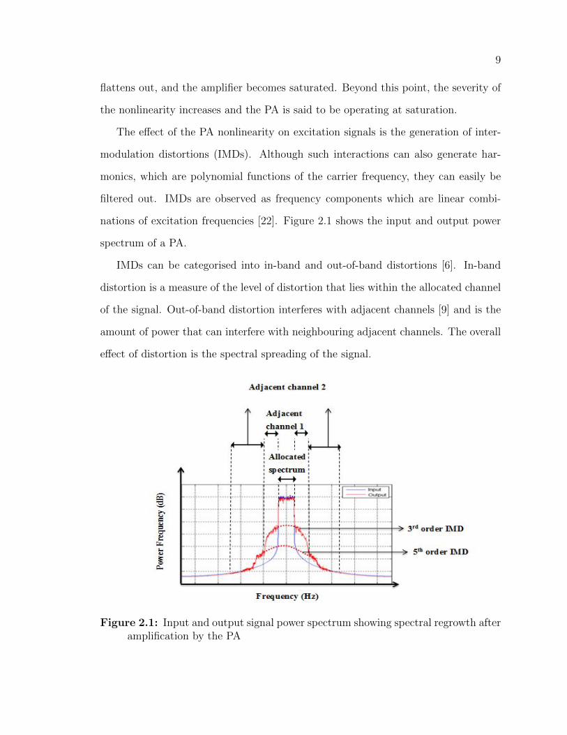
The effect of the PA nonlinearity on excitation signals is the generation of inter-

modulation distortions (IMDs). Although such interactions can also generate har-

monics, which are polynomial functions of the carrier frequency, they can easily be

filtered out. IMDs are observed as frequency components which are linear combi-

nations of excitation frequencies [22]. Figure 2.1 shows the input and output power

spectrum of a PA.

IMDs can be categorised into in-band and out-of-band distortions [6]. In-band

distortion is a measure of the level of distortion that lies within the allocated channel

of the signal. Out-of-band distortion interferes with adjacent channels [9] and is the

amount of power that can interfere with neighbouring adjacent channels. The overall

effect of distortion is the spectral spreading of the signal.

Figure 2.1: Input and output signal power spectrum showing spectral regrowth afteramplification by the PA

10

Signals generated using advanced and complex modulation schemes, such as the

Wideband Code Division Multiple Access (WCDMA) technique, possess high PAPR,

drive the power amplifier to saturation and are highly sensitive to PA nonlinearities

[8, 23]. These signals have non-constant envelopes and enable PAs to operate near

saturation with improved efficiencies.

In addition to the nonlinearity imposed by the PA on wideband signals, the signals

cause the PA to exhibit memory effects. Wider bandwidth signals tend to increase

the memory effect exhibited by the PA. In such cases, the response of the PA is

affected by the frequency of the input signal and not only its amplitude. Based on

this, PA nonlinearity is classified into memoryless nonlinearities and memory-based

nonlinearities.

Past inputs affect the present nonlinear effect for memory-based nonlinearities.

This means that memory nonlinearities increase the number of parameters for mod-

eling the IMDs. The severity of the memory effect on the PA increases as the number

of carriers or bandwidth of the excitation signal increases. The memory effect in a

PA usually appears in the input-output power plot, shown in Figure 2.2, as hysteresis

and dispersions.

(a) Memoryless PA (b) PA with memory

Figure 2.2: Input-Output power relationship of (a) memoryless nonlinear PA and(b) memory nonlinear PA

11

2.3 Power Amplifier Characterization

It is essential to characterize the distortions caused by the PA in order to adequately

compensate for its nonlinearities. The PA is characterized to determine the relation-

ship between the input and the output signal. This characterization specifies the

behavior of the PA in terms of the degree of its nonlinearity and the depth of the

memory effect it experiences.

Nonlinearity characterization of a PA can be done through testing by sweeping

signals across the PA. These tests provide a good understanding of the amplitude-

amplitude (AM/AM) distortions, amplitude-phase (AM/PM) distortions, and in-

band and out-of-band intermodulation distortions exhibited by the PA. Linearity

specifications, such as Adjacent Channel Power Ratio (ACPR) and Normalised Mean

Square Error (NMSE), are also given to characterize and measure the degree of the

unwanted signal generated by the PA.

A third order polynomial given in Equation 2.1 describes the input/output char-

acteristics of a nonlinear PA.

Y = b1X + b2X2 + b3X

3 (2.1)

where X and Y represent the input and output signals respectively. The bi terms

represent the real or complex-valued coefficients. The first order term specifies the

gain of the PA and is the only term for a linear PA. The second and third order terms,

represent the quadratic and cubic nonlinearities respectively.

For a continuous wave (CW) one-tone characterization, an input signal X(t), can

be written as

X(t) = A sin(wt) (2.2)

12

where A and w represent the amplitude and the frequency of the signal respectively.

The resulting output of the PA using Equation 2.2 as input gives

Y = b1(A sin(wt)) + b2(A sin(wt))2 + b3(A sin(wt))3 (2.3)

The expansion of the terms in Equation 2.3 produces Equation 2.4 which can be

re-written simply as Equation 2.5

Y = b1A sin(wt) + b2A2

2− b2

A2

2cos(2wt) + 3b3

A3

4sin(wt)− b3

A3

4sin(3wt) (2.4)

Y = a sin(wt) + b − b cos(2wt) + c sin(wt)− d sin(3wt) (2.5)

The second term of Equation 2.3 generates a DC term and a 2nd order harmonic

which are the second and third terms of Equation 2.4 respectively. These terms

distort the output signal and appear as out-of-band distortions. The third term

of Equation 2.3 generates an in-band distortion at the fundamental frequency and

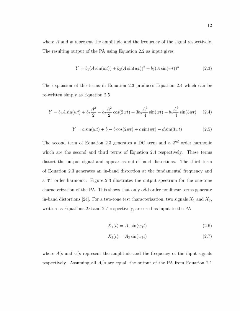
a 3rd order harmonic. Figure 2.3 illustrates the output spectrum for the one-tone

characterization of the PA. This shows that only odd order nonlinear terms generate

in-band distortions [24]. For a two-tone test characterisation, two signals X1 and X2,

written as Equations 2.6 and 2.7 respectively, are used as input to the PA

X1(t) = A1 sin(w1t) (2.6)

X2(t) = A2 sin(w2t) (2.7)

where A′is and w′is represent the amplitude and the frequency of the input signals

respectively. Assuming all Ai′s are equal, the output of the PA from Equation 2.1

13

Figure 2.3: Output spectrum for a one-tone characterization. Adapted from [1]

can be written as

Y = b1A(sin(w1t) + sin(w2t)) + b2A2(1 + cos((w2 − w1)t)

+9b3A

3

4(sin(w1t) + sin(w2t))

+3b3A

3

4(sin((2w1 − w2)t) + sin((2w2 − w1)t))

− b2A2(cos((w1 + w2)t)−b3A

3

4(sin(3w1t)− sin(3w2t))

− 3b3A3

4(sin((2w1 + w2)t)− sin((2w1 − w2)t)) (2.8)

Figure 2.4 shows the output frequency components (in-band and out-of-band dis-

tortions) generated using the two-tone test. The one-tone characterization is inac-

curate as it fails to completely identify the distortions that the PA can impose on

a signal [25, 26]. The two-tone characterization is more accurate than the one-tone

characterization. However, it does not capture the full behavior of the PA especially

when excited by signals with wider bandwidth. Memory effects exhibited by wide-

band signals are neglected by these traditional characterizations and this makes it

14

Figure 2.4: Output frequency spectrum from a two-tone characterization.

insufficient for PA characterization. Thus, it is necessary to characterize the PA with

signals it will experience in practice that can provide complete modeling of the PA

nonlinear behavior.

2.3.1 Amplitude and Phase Distortions

The effect of changes in the amplitude of the input on the output amplitude and phase

can characterize the nonlinear PA. Two effects that can characterize the nonlinear

PA are: 1) the amplitude-amplitude (AM/AM) distortion and 2) the amplitude-phase

(AM/PM) distortion. The AM/AM characteristic specifies the changes in the output

amplitude power due to changes in the input amplitude power level. The AM/PM

is the variation in the phase of the output signal according to the changes in the

amplitude of the input signal.

The graphical illustration of these two effects are referred to as the characteristic

plots. Figure 2.5 shows the AM/AM and AM/PM characteristic plots of a PA. The

15

x and y coordinates of the AM/AM and AM/PM plots can be derived as

AMx = 20log10|x(n)|

AMy = 20log10

{|y(n)||x(n)|

} (2.9)

APx = 20log10|x(n)|

APy = ∠y(n)∠x(n)

(2.10)

where AM and AP are the AM/AM and AM/PM respectively, x(n) is the input

signal, and y(n) is the output signal.

Figure 2.5: AM/AM and AM/PM characteristic plots for a PA.

2.3.2 Adjacent Channel Power Ratio

An important metric to characterize the PA behavior is the Adjacent Channel Power

Ratio (ACPR). The ACPR specifies the amount of spectral regrowth in adjacent

channels surrounding the main allocated channel. ACPR is the comparison between

the power in the adjacent channels and power in the required signal’s channel. The

ACPR is calculated as

16

ACPR = maxm=1,2...

∫(adj)m

|Y (f)|2df∫ch

|Y (f)|2df(2.11)

where Y(f) is the discrete fourier transform of the signal. The integral∫

(adj)m

measures

the power in each m number of upper and lower adjacent channels close to the main

channel. The integral∫ch

measures the power in the main channel. The maximum

ACPR value from all m adjacent channels is selected as the ACPR measurement.

2.3.3 Normalised Mean Square Error

The NMSE compares the measured output signal and the estimated output signal

from a model of the PA in the time domain. The NMSE evaluates the in-band

distortions of the PA and the accuracy of the estimated time domain output signal

of a PA model. The NMSE can be calculated using Equation 2.12 given as

NMSE [dB] = 10log10

∑n

|y(n)− y(n)|2∑n

|y(n)|2

(2.12)

where y(n) and y(n) represent the measured output and estimated model output

signals of the PA respectively.

The typical linearity requirements of a PA specified by the 3GPP standard [10]

for wideband signals are

• ACPR at 5MHz must be lesser than −45dBc and −50dBc at 10MHz.

• NMSE should be lesser than −35dB.

17

2.4 PA Modeling

Accurate modeling of the distortions which the PA imposes on a signal while inter-

acting with it, is critical for the synthesis of an effective digital pre-distorter. This is

because ideally, the pre-distorter should possess complete knowledge and/or estimates

of all the distortions and memory effect it is required to compensate for.

Several methods for modeling the behavior of a nonlinear system such as the PA

exists. Examples of modeling methods include the physics-based and the system-level

models. Physical models require theoretical rules describing the interactions between

electronic components that make up the PA [6]. System-level models, otherwise

known as behavioural models, help to simplify the problem of modeling, because it

requires little knowledge of the PA circuit and hardware functionality.

Behavioral modeling can do without a priori information and only requires the

input and output data from the system. The system is taken as a device under test

(DUT) represented by a model seen as a black box. A mathematical equation specifies

the relationship between the input and output of the black box. These equations used

to represent the DUT can define its characteristics in different ways termed as model

structures. Figure 2.6 illustrates the PA as a black box.

Figure 2.6: PA as a black box device under test

18

The two classes of behavioral models for nonlinear systems reported in the lit-

erature are memoryless and memory based models. The classification is based on

their ability to represent the PA memory effects. It is worth mentioning that no best

model exists [14] as modeling depends on factors such as the specific type of PA and

its excitation signal. The appropriate model selection is based on the model that is

good enough to estimate the behavior of the specific device under test.

2.4.1 Memoryless Nonlinear Models

A memoryless nonlinear model has its output as a function of only the present input.

They are usually referred to as frequency independent nonlinear models. Current

systems employing wideband signals do not use memoryless model structures to rep-

resent the PA because they fall short of capturing the memory effects exhibited by

wideband signals having wider bandwidth. A few memoryless models exist in the

literature such as the Saleh model [27, 28], the look-up table model [2, 17] and the

memoryless polynomial model [27,29].

Saleh [28] proposed a nonlinear model that characterises the behavior of the PA

as shown in Equation 2.13

y(n) =αa|x(n)|

1 + βa|x(n)|2exp{j αb|x(n)|2

1 + βb|x(n)|2} (2.13)

where αa, αb, βa and βb are the parameters of the model that describe the AM/AM

and AM/PM distortions and x(n) and y(n) are the input and output of the PA

respectively. The memoryless polynomial models approximates the PA behavior as a

summation of polynomials written as

y(n) =K∑k=1

bk|x(n)|k−1x(n) (2.14)

19

where x(n) and y(n) are the input and output of the PA respectively, bk are the

complex valued coefficients and K is the highest order of the polynomial model.

This thesis focuses on wideband signals, which require the use of memory models.

Therefore, further information on memoryless models is not provided.

2.4.2 Memory Nonlinear Models

Memory effects or dynamic distortions [17] cause the output of the PA to be a function

of previous input samples together with current ones. Several memory models with

differing levels of complexity have been proposed. These include: Voltera series, twin-

box, memory polynomial, and generalised memory polynomial models. Others are:

the nonlinear auto-regressive moving average (NARMA) model structure [30], the

dynamic deviation reduction (DDR) based Volterra series model [31], artificial neural

network (ANN) based model [1] and the look-up table (LUT) model structures. As

no perfect model exists, model structure selection is based on a specific application

and the power level of operation of the PA.

Volterra Series Model

The Volterra series is a popular and comprehensive nonlinear model capable of ac-

curately modeling dynamic nonlinear systems [17, 27]. One major drawback of this

complex model is the large number of parameters that are required to be estimated.

Equation 2.15 shows the input-output relationship of the Volterra model.

y(n) =K∑k=1

M∑i1=0

...M∑

ik=0

hk(i1, ..., ik)K∏j=1

x(n− ij) (2.15)

where hk(i1, ..., ik) are the parameters of the model, K is the nonlinearity order and

M is the memory depth. The model is well suited for mild nonlinearity. In the face

20

of strong nonlinearity, the Volterra model will require a large number of parameters.

Other variants of the Volterra series with reduced complexity (number of parameters)

and comparable performance have been developed in [13,30–32].

Twin-box Models

Twin box models are a combination of a linear time-invariant (LTI) system with an

impulse response function as Equation 2.16, followed by a memoryless nonlinearity

given in Equation 2.17. This model assumes that memory effects are linear and can

be decoupled from the nonlinear system [32]. One disadvantage of the Wiener (Figure

2.7(a)) and Hammerstein models (Figure 2.7(b)) is the fact that the output depends

nonlinearly on the coefficients. Estimation of coefficients becomes more difficult in

the twin-box models compared to models that are linear in the parameters [13].

(a) Wiener model

(b) Hammerstein model

Figure 2.7: Twin box models

The combination of the Wiener and Hammerstein models seeks to improve upon

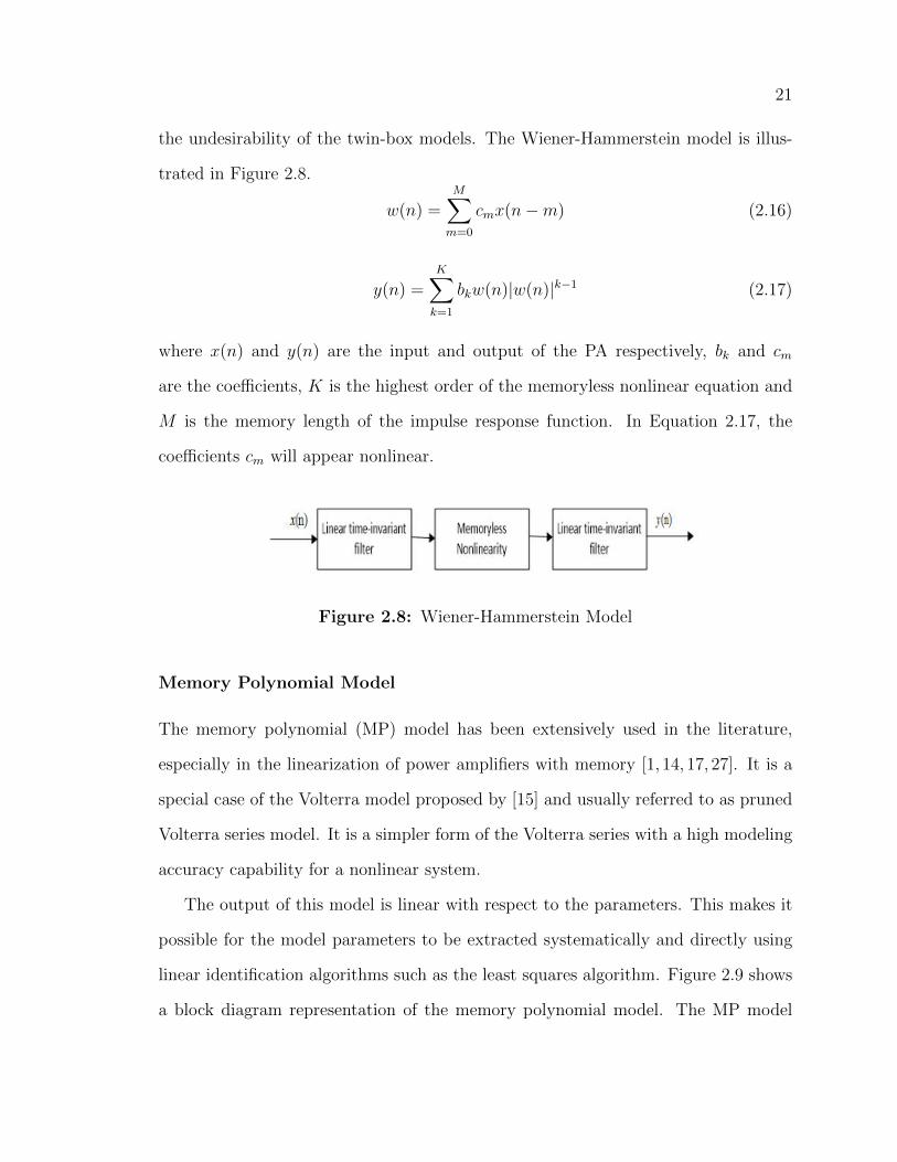
21

the undesirability of the twin-box models. The Wiener-Hammerstein model is illus-

trated in Figure 2.8.

w(n) =M∑

m=0

cmx(n−m) (2.16)

y(n) =K∑k=1

bkw(n)|w(n)|k−1 (2.17)

where x(n) and y(n) are the input and output of the PA respectively, bk and cm

are the coefficients, K is the highest order of the memoryless nonlinear equation and

M is the memory length of the impulse response function. In Equation 2.17, the

coefficients cm will appear nonlinear.

Figure 2.8: Wiener-Hammerstein Model

Memory Polynomial Model

The memory polynomial (MP) model has been extensively used in the literature,

especially in the linearization of power amplifiers with memory [1, 14, 17, 27]. It is a

special case of the Volterra model proposed by [15] and usually referred to as pruned

Volterra series model. It is a simpler form of the Volterra series with a high modeling

accuracy capability for a nonlinear system.

The output of this model is linear with respect to the parameters. This makes it

possible for the model parameters to be extracted systematically and directly using

linear identification algorithms such as the least squares algorithm. Figure 2.9 shows

a block diagram representation of the memory polynomial model. The MP model

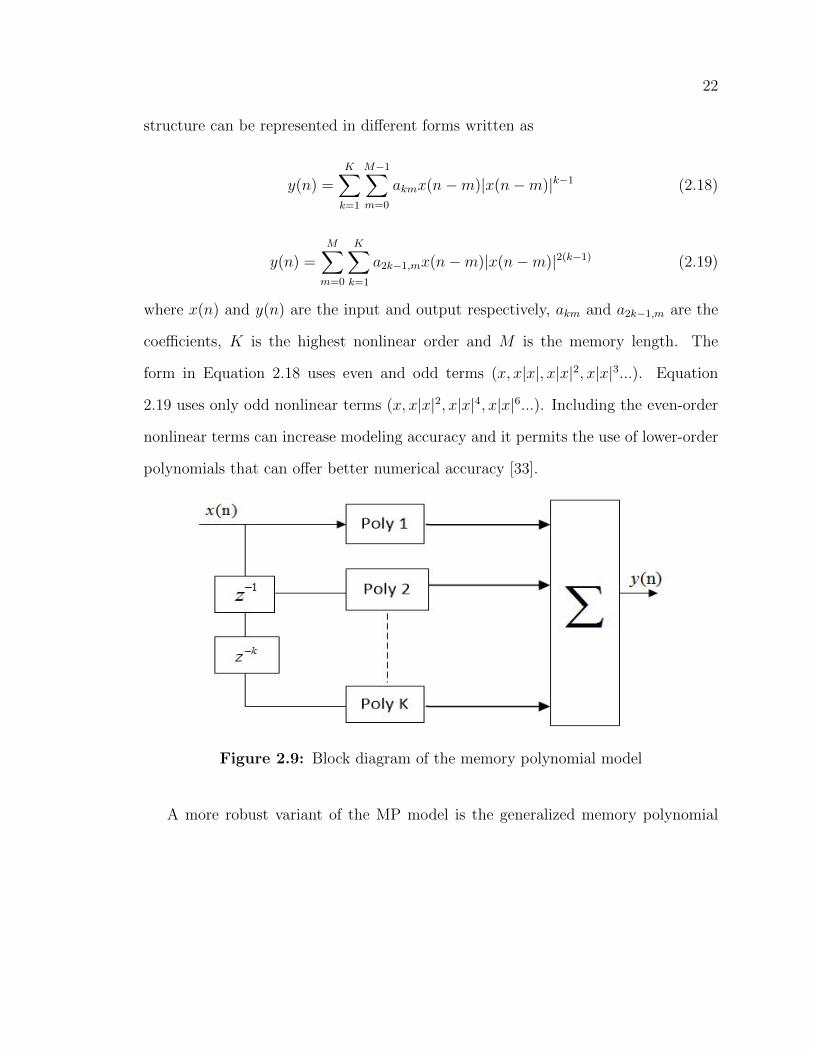
22

structure can be represented in different forms written as

y(n) =K∑k=1

M−1∑m=0

akmx(n−m)|x(n−m)|k−1 (2.18)

y(n) =M∑

m=0

K∑k=1

a2k−1,mx(n−m)|x(n−m)|2(k−1) (2.19)

where x(n) and y(n) are the input and output respectively, akm and a2k−1,m are the

coefficients, K is the highest nonlinear order and M is the memory length. The

form in Equation 2.18 uses even and odd terms (x, x|x|, x|x|2, x|x|3...). Equation

2.19 uses only odd nonlinear terms (x, x|x|2, x|x|4, x|x|6...). Including the even-order

nonlinear terms can increase modeling accuracy and it permits the use of lower-order

polynomials that can offer better numerical accuracy [33].

Figure 2.9: Block diagram of the memory polynomial model

A more robust variant of the MP model is the generalized memory polynomial

23

(GMP) [13]. The model can be written as

y(n) =Ka−1∑k=0

La−1∑l=0

aklx(n− l)|x(n− l)k+

Kb∑k=1

Lb−1∑l=0

Mb∑m=1

bklmx(n− l)|x(n− l −m)|k+

Kc∑k=1

Lc−1∑l=0

Mc∑m=1

cklmx(n− l)|x(n− l +m)|k (2.20)

where x(n) and y(n) are the input and output respectively, KaLa represents the num-

ber of coefficients similar to those of the MP model, KbLbMb are the number of coef-

ficients for lagging envelope and signal, and KcLcMc represents the number of coeffi-

cients for the signal and leading envelope. The cross-terms,(x(n)|x(n−1)|, x(n)|x(n−

2)|, x(n−1)|x(n−2)...), can be estimated using linear estimating algorithms and this

gives favorable implications for algorithm stability and computational complexity.

This thesis uses the MP model structure for fitting the characteristics of the PA

and its inverse from measured input and output. Polynomial models have showed

good performance when used with weak or high nonlinear PA [14]. The number of

parameters are not as much as the Volterra series model and they can be estimated

using linear model identification algorithms.

Chapter 3

Adaptive Digital Pre-distortion

3.1 Introduction

Digital pre-distortion is a technique used for the linearization of power amplifiers.

It has the capability to improve the linearity and efficiency of PAs. DPD uses the

inverse models of power amplifiers to control the output of the PA. This approach is

referred to as inverse modeling. When the operating condition of a PA changes, the

output of the PA may experience different levels of distortion. Therefore, adaptive

DPD can maintain the desired output of the PA.

At present, several adaptive DPD schemes exist. The scheme proposed in this

thesis is intended to maintain the linearity of PAs through faster adaptation, re-

duced transient errors and reduced complexity. This chapter reviews the concept of

pre-distortion, inverse modeling, adaptive DPD and model identification algorithms.

Adaptive DPD schemes are also reviewed.

24

25

3.2 Pre-distortion

Pre-distortion is the introduction of distortion to the input signal before its interaction

with a PA. A pre-distorter (PD) is a nonlinear block with an inverse characteristic of

the PA [6]. The purpose of the PD is to introduce a complementary nonlinearity to

an input signal that can cancel out the intrinsic nonlinearity of the PA [11]. Figure

3.1 illustrates the concept of pre-distortion. The pre-distorter is inserted prior to

the PA to invert the gain characteristic of the PA. The PD introduces an expansive

distortion to the signal which is cancelled by the compressive distortion introduced

by the PA.

Figure 3.1: Pre-distortion scheme

The PA output yp and the PD output yd can be given as

yp = xp.G(|xp|) (3.1)

yd = xd.F (|xd|) (3.2)

where G(|xp|) and F (|xd|) denote the AM-AM and AM-PM characteristics of the PA

and PD respectively. Whereas, xp and xd represent the input signal of the PA and

26

PD respectively. The terms yp, xp, yd, xd, G(|xp|) and F (|xd|) are all in complex form.

The output of the cascade of the PA and PD is given as

yp = xd.F (|xd|).G(|xd.F (|xd|)|) (3.3)

Overall, the output of the linearized PA can be written as

yp = A.xd (3.4)

where A, yp and xd represents the gain, output and input signal of the linearized PA

respectively.

The PD can be implemented in analog at intermediate frequency (IF) or in digital

form at baseband using digital signal processing (DSP) techniques. The pre-distortion

achieved at baseband is referred to as baseband digital pre-distortion (DPD). Im-

plementing pre-distortion with DSP at baseband is usually preferred because it re-

duces cost, and enjoys flexibility [34], and is better suited for realising adaptive pre-

distorters [16, 19, 23]. The work reported in [23] showed that a digital pre-distorter

offered better linearization performance than other analog pre-distorters.

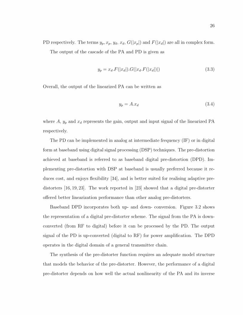
Baseband DPD incorporates both up- and down- conversion. Figure 3.2 shows

the representation of a digital pre-distorter scheme. The signal from the PA is down-

converted (from RF to digital) before it can be processed by the PD. The output

signal of the PD is up-converted (digital to RF) for power amplification. The DPD

operates in the digital domain of a general transmitter chain.

The synthesis of the pre-distorter function requires an adequate model structure

that models the behavior of the pre-distorter. However, the performance of a digital

pre-distorter depends on how well the actual nonlinearity of the PA and its inverse

27

Figure 3.2: Diagrammatic representation of digital pre-distortion

function are modeled to match their true characteristics. The relationship between

the input and output of the pre-distorter can be determined using models.

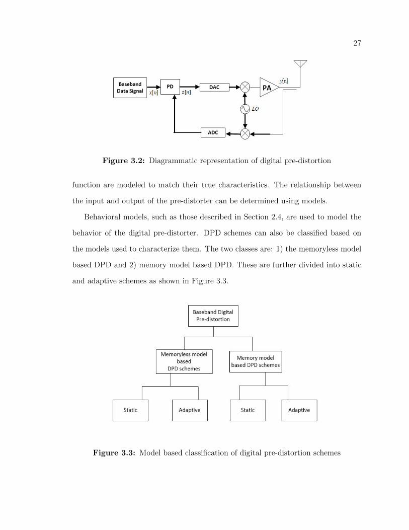
Behavioral models, such as those described in Section 2.4, are used to model the

behavior of the digital pre-distorter. DPD schemes can also be classified based on

the models used to characterize them. The two classes are: 1) the memoryless model

based DPD and 2) memory model based DPD. These are further divided into static

and adaptive schemes as shown in Figure 3.3.

Figure 3.3: Model based classification of digital pre-distortion schemes

28

The memory based schemes can capture the memory effects exhibited by the

wideband signals while the memoryless schemes cannot capture memory effects. The

characteristics of the model specified by the parameters of the model structure can

then be estimated using identification algorithms. As mentioned earlier, memory

based schemes are considered because wideband signals are used in this thesis.

3.3 Inverse Modeling

Inverse modeling is described as the method by which a model uses its inverse to

control itself. This approach reduces the difference between the input and output of

the system. The inverse of a model can be applied before or after the model to be con-

trolled. Application of the inverse model before and after is referred to as pre-inverse

and post-inverse respectively. Figure 3.4 shows the diagrammatic representation of

the concept of pre- and post-inverse modeling. The method chosen to estimate the

inverse of a system has a large impact on the result of the cascade of the inverse

model and the model to be controlled. Inverse modeling is used in DPD for control

and linearization of the PA.

One common problem with the pre- and post-inverse methods is finding the inverse

model itself. There are different methods for estimating a system’s inverse. These

include inversion by feedback, analytic inversion, and inversion by system simulation

[35]. Inversion by feedback requires that a model that characterises the PA is selected.

The model of the PA is estimated and inverted to generate the inverse model, the

PD.

Analytic inversion uses an ideal pre-distorter to obtain an estimate. The PA model

is estimated and the PD model is placed in series with the PA. The parameters are

estimated based on the error between the input and the output of the PA and PD

29

(a) Pre-inverse

(b) Post-inverse

Figure 3.4: Inverse control methods

combination. This is termed the direct learning architecture (DLA) [15]. The same

model structures can be used for the PA and the PD or the PA model structure can

be more complex. In DLA, the predistorter is obtained by direct pre-inversion of the

PA characteristics. Figure 3.5 illustrates the direct learning architecture.

Figure 3.5: Direct learning architecture

30

Inversion by system simulation estimates the inverse of the PA directly without a

PA model. Input and output data are used directly to identify the inverse model. This

is termed as the indirect learning architecture (ILA) [14]. For the ILA, a post-inverse

of the nonlinear model is derived and then transferred for use as a pre-distorter.

Figure 3.6 illustrates the indirect learning architecture. A PD implemented using the

ILA proposed in [14] achieved a robust linearization performance because the memory

polynomial structure based pre-distorter was not tied to a particular PA model.

Figure 3.6: Indirect learning architecture

In this thesis, the indirect learning architecture is the inverse modeling method

of choice. The basis for this is because it is more commonly used than the direct

learning architecture and the inverse can be estimated directly.

3.4 Memory Model Based Digital Pre-distortion

Schemes

Static memory model based DPDs, sometimes referred to as open-loop DPD architec-

ture, can be suitable for PAs with small dynamic ranges. They are effective when the

31

PA’s input-output characteristics are nonvarying. Figure 3.7 shows the diagrammatic

representation of the static pre-distorter scheme. The characteristics of the PA and

DPD can be estimated using an estimation algorithm such as the Least Squares (LS)

algorithm. This estimation is a one-time estimation done offline.

Figure 3.7: Block diagram of a static DPD scheme

The nonlinear behaviour of the PA depends on the statistics of its input signal

[5, 36]. The AM/AM and AM/PM distortions are functions of the input signal and

different levels of distortions can be obtained for different excitation signals. Thus,

static DPD cannot compensate for the changing characteristics exhibited by the PA.

Adaptive DPDs can compensate for the nonlinearities of a PA in real time [34]

and continuously update the coefficient of the DPD. They are capable of tracking

possible changes in the PA behavior by getting feedback from the PA’s output. The

adaptation is based on the difference between the desired output and the PA’s actual

output.

Adaptive DPD schemes can employ adaptive filtering algorithms that estimate

the pre-distorters coefficient .Adaptation can also be performed through the use of a

look-up table (LUT) [37,38]. A complex polynomial generates and updates the entries

of the LUT and the parameters of the PD model are drawn and updated from the

32

LUT. For the former, polynomial-based adaptation algorithms such as Least Mean

Squares (LMS) and Recursive Least Squares (RLS), are used for the identification and

continuous update of the model parameters. Figure 3.8 shows the generic polynomial-

based adaptive scheme for PA linearization. The LUT-based adaptive scheme is very

Figure 3.8: Block diagram of a polynomial-based adaptive DPD

flexible and has high accuracy. An increase in the number of LUT entries increases

the accuracy of the estimated model. However, the complexity of the scheme increases

as the number of LUT entries increases. Thus, performance trade-offs exist with the

LUT-based adaptive DPD schemes. Figure 3.9 shows a gain-based LUT adaptive

DPD scheme.

Figure 3.9: Block diagram of a gain-based LUT adaptive DPD. Adapted from [2]

33

For all adaptive algorithms, coefficients of the PD model are updated by com-

parison between the original excitation signal at the PDs input, and the PA output.

This is carried out on a sample-by-sample basis and the size of the estimation error is

monitored to continuously minimize it. The error is used in the adaptation algorithm

to control the system. A comparison of the polynomial and LUT-based adaptations

reported in [19] showed that the polynomial-based adaptation algorithms provided

better performance in terms of convergence time and error than the LUT-based adap-

tation. This work focuses on the use of polynomial-based memory model adaptive

pre-distortion.

3.5 Model Parameters Identification and Estima-

tion Algorithms

Model parameters are extracted using identification algorithms that make use of the

input data and the corresponding output data from the system to be identified. The

accuracy of the estimated output of the model depends on the model structure chosen

and the parameter extraction algorithm used. Most of these models are approximates

of the complex Volterra series model and this makes the quality of the behavioral

model depend on the parameter extraction process rather than the model structure

[39]. The main algorithms for extracting model parameters obtained from real time

data measurements are: least squares (LS), least mean squares (LMS), and recursive

least squares(RLS).

34

3.5.1 Least Squares Algorithm

The least squares (LS) algorithm is used for a one-time parameter estimation of a

model. It finds the best set of parameters for a model using a given set of data

points by minimizing the sum of the squares of the residuals between the true system

output and the model’s output estimates. Equation 3.5 describes the model structure

associated with the memory polynomial model of a nonlinear system.

y(n) =K∑k=1

M−1∑m=0

akmx(n−m)|x(n−m)|k−1 (3.5)

where x(n) and y(n) are vectors containing the input and output data samples, M is

the memory depth and K is the nonlinear order. The variable n denotes the sample

index Equation 3.5 can be written as:

y(n) = φ(n)θ (3.6)

φ(n) =

x10 · · · x1(M−1) · · · x11|x11|K−1 · · · x1(M−1)|x1(M−1)|K−1

x20 · · · x2(M−1) · · · x21|x21|K−1 · · · x2(M−1)|x2(M−1)|K−1...

...... · · · ...

......

xN0 · · · xN(M−1) · · · xN1|xN1|K−1 · · · xN(M−1)|xN(M−1)|K−1

(3.7)

θT =

[a10 · · · a1(M−1) a20 · · · a2(M−1) · · · aK0 · · · aK(M−1)

](3.8)

where φ(n) is the regression matrix formed from all the present and past inputs written

as Equation 3.7 and θ is the vector containing unknown complex-valued parameters

of the model written as Equation 3.8.

35

The least squares solution gives the estimate of the model parameters and is

computed as

θ = φ+(n)y(n) (3.9)

where φ+(n) is the pseudoinverse of φ(n) given as

φ+(n) = (φH(n)φ(n))−1φH(n) (3.10)

H represents the hermitian or complex conjugate transpose. The estimate of the

model output is computed as

y(n) = φ(n)θ (3.11)

The model parameters estimated are chosen to minimize the prediction error e(n)

between the actual output y(n) and the estimated output y(n) given as

e(n) = y(n)− y(n) (3.12)

The accuracy of the model and the estimated parameters associated with the estima-

tion is evaluated using the Normalised Mean Square Error (NMSE) metric computed

as Equation 2.12 in Section 2.3.3. The NMSE value determines to what extent the

model fits the data. A small NMSE value is an indication of a good estimate.

3.5.2 Adaptive Algorithms

Stochastic gradient algorithms (LMS) and sample-by-sample based adaptive estima-

tion algorithms (RLS) are examples of adaptive algorithms employed for adaptive

digital control. Each of these algorithms differ in performance, convergence speed

36

and computation complexity. The performance, accuracy and stability of these algo-

rithms affect the overall performance of the adaptive DPD scheme.

I Least Mean Squares (LMS)

The parameters of a model given as Equation 3.5 and 3.6 can be determined online

using the least mean squares (LMS) algorithm. The model parameters, θ (Equation

3.8) are continuously adjusted to minimize e(n) given as

e(n) = y(n)− y(n) (3.13)

where y(n) and y(n) are the actual and estimated output respectively and n is the

sample index. y(n) is given as

y(n) = φ(n)θn (3.14)

The algorithm computes the current parameters using:

θn+1 = θn + (µ ∗ φT (n) ∗ e(n)) (3.15)

where φ(n) is the regression matrix, θn are the parameters using previous n samples,

θn+1 are related to current n + 1 samples, µ is the step size and (.)T denotes the

transpose operator. The current parameter, θn+1, is based on previously estimated

parameters, θn, and e(n). The step size µ is chosen such that

0 < µ <2

λmax

(3.16)

where λmax is the maximum eigenvalue of the covariance matrix ρ derived as

ρ = E[φ(n)φT (n)

](3.17)

37

where φ(n) is the regressor vector, E[.] represents the mean and λmin is the minimum

eigenvalue of the covariance matrix. The condition number of the covariance matrix

tells how good an estimation is. A small condition number indicates a well conditioned

system and a good estimate can be determined. The illconditioning of this matrix

will generate a bad model estimate. The condition number is defined as

⊂=λmax(ρ)

λmin(ρ)(3.18)

II Recursive Least Squares (RLS)

The set of Equations 3.19 to 3.21 describe the RLS algorithm used to estimate the

parameters, θ, of a model given as Equation 3.5.

θn = θn−1 + L(n)(y(n)− φ(n)θn−1) (3.19)

L(n) =P (n− 1)φT (n)

λ+ φT (n)P (n− 1)φ(n)(3.20)

P (n) =P (n− 1)− L(n)φ(n)P (n− 1)

λ(3.21)

where x(n) and y(n) are vectors of length N containing the input and output data

respectively, L(n) is the gain vector, P (n) is the covariance matrix of the estimate

and λ is the forgetting factor.

The RLS algorithm uses changes in the error to track and update the model

parameters. The parameters that minimize the prediction error e(n) such that

e(n) = y(n)− y(n)

y(n) = φ(n)θ(n− 1)

e(n) = y(n)− φ(n)θ(n− 1)

(3.22)

38

where y(n) and y(n) are the actual and estimated output respectively, n is the time

step, and θ(n− 1) is the vector of the parameters using (n− 1) samples.

The forgetting factor λ allows the RLS algorithm to track changing parameters

by discounting old data. λ can be chosen such that

0.95 <λ< 1 (3.23)

If λ is close to 0.95, RLS algorithm will be able to track parameter changes quickly. If

close to 1, estimates change slowly. The covariance matrix P (n) is defined as pI where

I is an identity matrix with rows and columns equal to the number of parameters

to be estimated. The term p ∈ < is chosen based on how well the parameters are

known. The value p ranges from 0 to an arbitrarily large value. A p value of 0 is

chosen when the parameters are well known otherwise, a large p value is used.

3.6 Review of Adaptive Digital Pre-distortion

Schemes

Adaptive pre-distorter schemes are intended to linearize the output of PAs. Their

performance can be measured in terms of speed, complexity and stability. The speed

of the pre-distorter is determined by: 1) the time taken at startup for the parameters

to converge to values close to the true values for the unknown DPD model and 2) the

time taken for the parameters to reconverge after sudden changes in the PA behavior.

Complexity depends on the number of computations that are required in the pre-

distorter scheme. Complexity is also determined by the number of samples processed

at every estimation and behavioral change. Stability is a measure of how well the

parameters transition to the true values at every estimation.

39

One of the earliest adaptive PDs reported by [21] offered precise compensation

for the nonlinear distortions and adapted to the changes of the PA. The adaptive

LUT-based DPD scheme proposed in [17] showed a reduction in convergence time,

reconvergence time and complexity compared to [21]. The cascade of a LUT PD

and piecewise pre-equalisers proposed in [40] improved on the the LUT-based Ham-

merstein PD. This method corrected all types of memory effects and simplified the

hardware implementation.

An adaptive pre-distorter with a modified LMS algorithms was presented in [29].

A third and fifth order adaptive pre-distorter scheme reported in [16] used a one-

dimentional search adaptation algorithm to improve the speed and complexity of

PAs. However, these adaptive schemes did not evaluate the performance of PAs with

fast load changes, especially changes experienced in a base station.

A learning module PD for adaptive PD implementation [41] evaluated with only

two discrete power level changes was reported to have rapid convergence of parameters

and the ability to learn from past experiences. The PD was demonstrated to improve

the transient error and provide implementation at low cost compared to conventional

adaptive schemes.

The authors in [7,42] proposed an adpative scheme to suppress distortions due to

power changes, but did not validate the scheme using large dynamic ranges. A power-

adaptive DPD approach, which avoided parameter recaliberation and eliminated PA

distortion due to large dyanmic changes was presented in [43].

3.7 Improvement to Adaptive DPD Schemes

Stochastic systems can experience rapid disturbances and multiple parameter changes.

Conventional adaptive control schemes for stochastic systems have large transient

40

errors during initial estimation and re-estimation of parameters as they transition

to their true values. A multiple model control scheme for a controller operating in

multiple environments [44] was shown to improve the transient response of the system.

Adaptive control can use multiple models to manage large transients with rapid

convergence [20,45,46]. A set of models can be used as opposed to a single model used

in conventional schemes. The models can have the same structure with equal number

of parameters or different structures with different required parameters. Likewise,

the same or different algorithms can be used to estimate the model parameters. The

model chosen at any instant must provide the best possible linearization performance.

Multiple models require a switching method between the set of models (bank of

models). The hypothesis test switching method presented in [47–49] has improved

stability than the heuristic performance index switching method proposed in [50].

In this thesis, the adaptive digital pre-distorter is required to provide acceptable

linearization performance for a PA. The PA experiences rapid behavioral changes as

a result of the changing excitation signal. The parameters of the DPD changes to

compensate for the different distortions. The objective is to linearize the PA with

increased speed and reduced complexity.

Multiple model adaptive DPD with a hypothesis test based switching method is

proposed and evaluated to offer significant improvements over existing conventional

adaptive schemes.

Chapter 4

Multiple Model Baseband Adaptive

Digital Pre-distortion

4.1 Introduction

This chapter explains the multiple model adaptive digital pre-distortion scheme pro-

posed in this thesis. It describes the data employed in the simulation of the DPD. The

modeling and simulation procedure of a static and an adaptive DPD are presented.

The synthesis of the multiple model DPD scheme is presented. It improves and

builds on the structure of the static and adaptive DPD. The hypothesis test switching

algorithm incorporated in the multiple model scheme is presented. The scheme is

evaluated based on its linearization performance, complexity and speed.

4.2 Data Signals Structure

The input and output data measured from a PA are required for synthesizing a base-

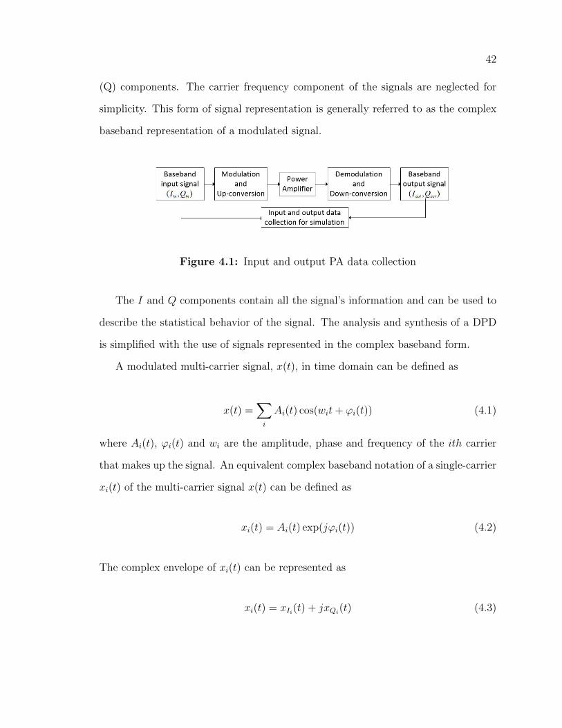
band DPD. Figure 4.1 shows the data collection process for the input and output of

a PA. These signals can be single-carrier or multi-carrier signals. In baseband, single-

or multi-carrier RF signals can be represented by their in-phase (I) and quadrature

41

42

(Q) components. The carrier frequency component of the signals are neglected for

simplicity. This form of signal representation is generally referred to as the complex

baseband representation of a modulated signal.

Figure 4.1: Input and output PA data collection

The I and Q components contain all the signal’s information and can be used to

describe the statistical behavior of the signal. The analysis and synthesis of a DPD

is simplified with the use of signals represented in the complex baseband form.

A modulated multi-carrier signal, x(t), in time domain can be defined as

x(t) =∑i

Ai(t) cos(wit+ ϕi(t)) (4.1)

where Ai(t), ϕi(t) and wi are the amplitude, phase and frequency of the ith carrier

that makes up the signal. An equivalent complex baseband notation of a single-carrier

xi(t) of the multi-carrier signal x(t) can be defined as

xi(t) = Ai(t) exp(jϕi(t)) (4.2)

The complex envelope of xi(t) can be represented as

xi(t) = xIi(t) + jxQi(t) (4.3)

43

where,

Ai(t) =√xIi(t)

2 + xQi(t)2

ϕi(t) = tan−1|xQi(t), xIi(t)|

(4.4)

The real (xIi(t)) and imaginary (xQi(t)) values of Equation 4.3 correspond to the

in-phase and quadrature components of the signal respectively. The modulated signal

xi(t) can be reproduced by multiplying the I and Q components by the cosine and

sine of the desired frequency respectively as shown in Equation 4.5.

xi(t) = xIi(t) cos(wit)− xQi(t) sin(wit) (4.5)

4.3 Characterization of the PA

The measured data signals define or determine the AM/AM and AM/PM characteris-

tics or response of the PA. Thus, these signals can be used to extract the parameters

of a model. The number of carriers, PAPR, and the average power of the signal

are used in this thesis, to define the statistics of the data. The average power of N

samples of I and Q data is defined as

Pavg = 10log10

[1

N

N∑n=1

|x(n)|2]

[dBm] (4.6)

where,

|x(n)| =√xI(n)2 + xQ(n)2 (4.7)

and n is the sample index. The PAPR of a signal is defined as

PPAPR = 10log10

max{|x(n)|2}1N

N∑n=1

|x(n)|2

[dB] (4.8)

44

where max{|x(n)|2} is the maximum {|x(n)|2} value computed for all the samples.

4.4 Time Delay Estimation and Alignment

The time resolution of the analog-to-digital conversion of the actual PA output signal

can result in a time delay between the digitized output and input signal of the PA [51].

It is important to synchronize the time of the measured PA input and output signals

and eliminate the time shift between the input and output signals.

The time delay of the PA data signals is estimated and synchronized before

the DPD synthesis, using the method proposed in [51]. The time delay estima-

tion/alignment approach presented in [51] applies a lagrange interpolation to the

input and output signals. This is done to improve the time resolution of the cross-

covariance estimated between the PA input and output signals. The Amplitude and

Pre-distorter Simulation Software (AMPS) is utilized to synchronize the PA signals.

The software follows the algorithm presented in [51].

4.5 Scaling of Output Data

The measured output data is scaled by a factor (SF ) that makes the linear gain of

the amplifier equal to 1 and replaces the 1SSG

term (SSG is the small signal gain of

the PA) after the PA. The scaled output yPAscaled(n) can be derived from the time

aligned measured output data ytimealignedPA(n) as

yPAscaled(n)=ytimealignedPA(n)× SF (4.9)

45

where,

SF =

1N

N∑n=1

(|xtimealignedPA(n)|

)1N

N∑n=1

(|ytimealignedPA(n)|

) (4.10)

and N is the number samples and SF = 1SSG

.

4.6 Data Pre-processing

The peak average power ratio (PAPR) of the pre-distorted signal (DPD output) is

higher than the PAPR of the actual PA input signal. Such phenomenon is referred

to as DPD avalanche [52]. However, the PA is characterized with the actual input at

its specific PAPR. When the PA is excited by the DPD’s output signal with a higher

PAPR, the PA is pushed more into saturation. Thus, the DPD in this case will only

degrade the achievable linearization performance of the PA.

Higher order polynomial-based models can improve the accuracy of the estimated

PA model. However, higher model orders increase the model parameters to be esti-

mated and the numerical instability of the model parameters causing large dispersions

in the parameters. Dispersions are the magnitude of the separation between the max-

imum and minimum parameter values.

The higher peaks and large parameter dispersions can be controlled and reduced

by pre-processing the data signals [38, 52–54]. The pre-processing of a signal x(n) is

described as

xpre−p(n) =x(n)− x

σ(4.11)

where x and σ are the mean and standard deviation of the signal x(n) respectively.

The notations, xPA(n) and yPA(n), that appear in the remaining sections of this

thesis represent the time-aligned, scaled and pre-processed input signal and output

46

signal respectively. It should be noted that the input signal is not scaled and the

pre-processing step operates on the time aligned input signal.

4.7 Static Digital Pre-distortion Synthesis

The synthesis structure is the procedure for realising DPD via simulation. Figure 4.2

illustrates the flowchart of a static DPD implementation via simulation. First, the

parameters of the PA and DPD model are estimated by an offline one-time model

identification algorithm that uses the input xPA(n), and output yPA(n) PA data. Sec-

ond, the PA input is passed through a cascade of the PA and DPD model (DPD+PA).

Figure 4.2: Flowchart for the static DPD implementation

The procedure below describes the synthesis of a static DPD:

47

• Let us assume that the characteristics of the PA and DPD can be described by

a polynomial model (MP) of the form

yPA(n) =

KPA∑k=1

MPA−1∑m=0

akmPAxPA(n−m)|xPA(n−m)|k−1 (4.12)

yDP (n) =

KDP∑k=1

MDP−1∑m=0

akmDPxDP (n−m)|xDP (n−m)|k−1 (4.13)

where xPA(n), yPA(n), akmPA, MPA, and KPA are associated with the PA model

while xDP (n), yDP (n), akmDP, MDP , and KDP are associated with the DPD

model. The signals x(n) and y(n) are the pre-processed input and output data

respectively, akm are the complex-valued model parameters, K is the highest

nonlinear order and M is the memory length of the model to be estimated.

The terms K and M specify the model configuration. The model structure is

the form of the mathematical representation of the PA and DPD model. It

should be noted that the PA model structure and configuration can be chosen

differently from that of the DPD. Table 4.1 shows the possible combinations of

a PA and DPD model structure and configuration.

Table 4.1: Possible PA and DPD model structure and configuration choice

Options Model Structure Model Configuration

Option 1 Identical IdenticalOption 2 Identical DifferentOption 3 Different IdenticalOption 4 Different Different

The optimum option uses the smallest configuration possible and the simplest

model structure that yields acceptable linearity with high speed and less com-

plexity.

48

• The LS algorithm described in Section 3.5.1 can be used for estimating the

parameters of the PA model. The parameters of the PA, akmPA, and the DPD,

akmDP, can be estimated as

akmPA= φPA

+(n)yPA(n) (4.14)

akmDP= φDP

+(n)yDP (n) (4.15)

where φPA+(n) and φDP

+(n) are the pseudoinverse of the regression matrix

φDP (n) and φDP (n) respectively. It should be noted that the PA’s input signal

xPA(n) becomes the DPD’s input signal xDP (n) while the PA’s output signal

yPA(n) becomes the DPD’s input signal yDP (n) for modeling the DPD.

• A cascade of the PA and DPD is desired to produce the linearized output,

ylinearizedPA(n), similar to the actual PA input. The actual PA input data,

xPA(n), is passed through the DPD to yield yDP (n). Then, yDP (n) serves as

the new PA input xnewPA(n). Equations 4.16 and 4.17 describe the derivation

of the linearized PA output.

yDP (n) =φPAT akmDP

= xnewPA(n) (4.16)

ylinearizedPA(n) =φnewPAT (n)akmPA

(4.17)

For a perfectly linearized PA,

ylinearizedPA(n) ' xPA(n) (4.18)

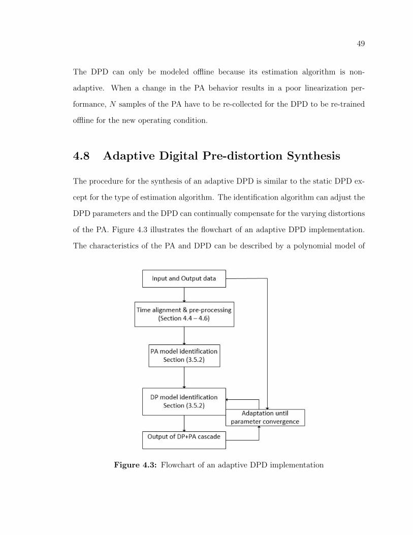
49

The DPD can only be modeled offline because its estimation algorithm is non-

adaptive. When a change in the PA behavior results in a poor linearization per-

formance, N samples of the PA have to be re-collected for the DPD to be re-trained

offline for the new operating condition.

4.8 Adaptive Digital Pre-distortion Synthesis

The procedure for the synthesis of an adaptive DPD is similar to the static DPD ex-

cept for the type of estimation algorithm. The identification algorithm can adjust the

DPD parameters and the DPD can continually compensate for the varying distortions

of the PA. Figure 4.3 illustrates the flowchart of an adaptive DPD implementation.

The characteristics of the PA and DPD can be described by a polynomial model of

Figure 4.3: Flowchart of an adaptive DPD implementation

50

the form

yPA(n) =

KPA∑k=1

MPA−1∑m=0

akmPAxPA(n−m)|xPA(n−m)|k−1 (4.19)

yDP (n) =

KDP∑k=1

MDP−1∑m=0

akmDPxDP (n−m)|xDP (n−m)|k−1 (4.20)

where xPA(n), yPA(n), akmPA, MPA, and KPA are associated with the PA model while

xDP (n), yDP (n), akmDP, MDP , and KDP are associated with the DPD model. The

terms x(n) and y(n) are the pre-processed input and output data respectively, akm

are the complex-valued model parameters, K is the highest nonlinear order and M

is the memory length of the model to be estimated.

The PA parameters, akmPA, and DPD parameters, akmDP

can be estimated using

akmPA(n+ 1) = akmPA

(n) + (µ ∗ φPAT (n) ∗ ePA(n)) (4.21)

akmDP(n+ 1) = akmDP

(n) + (µ ∗ φDPT (n) ∗ eDP (n)) (4.22)

The estimation error e(n) between the actual PA input xPA(n) and the estimated

output yDP+PA(n) of the cascade of the DPD and PA model, controls the algorithm.

The error e(n) is written as

e(n) =xPA(n)− yDP+PA(n) (4.23)

New xPA(n) and yPA(n) samples can cause large errors in the estimation of the DPD

parameters. The adaptive schemes described above are prone to large transient er-

rors and the linearization performance is poor. Large changes in parameters degrade

the linearization performance of the DPD. This requires larger sample sizes to be

processed before parameters converge to optimal values to achieve the linearity per-

formance specified by standards.

51

4.9 Multiple Model Digital Pre-distortion

The multiple model DPD scheme is intended to reduce the time taken for the DPD

to optimize its parameters for the present operating condition (start-up and during

system changes). Figure 4.4 shows a block diagram of the multiple model DPD

scheme. The scheme uses a set of DPD models (DPMi) each with its own set of

parameters. Each DPMi is related to a specific operating condition of the PA. The

parameters are grouped, stored and addressed in memory based on their power level

and bandwidth as shown in Figure 4.5.

Figure 4.4: Block diagram of the multiple model scheme

The DPD models are switched based on the operating condition of the PA and

related to the input signal statistics at any given instant. A hypothesis test based

switching algorithm is employed to determine model switching. When a switch is

initiated by the algorithm, a certain set of DPMi model parameters are selected. In

response to the selection of a DPMi model after the switching decision, the adaptive

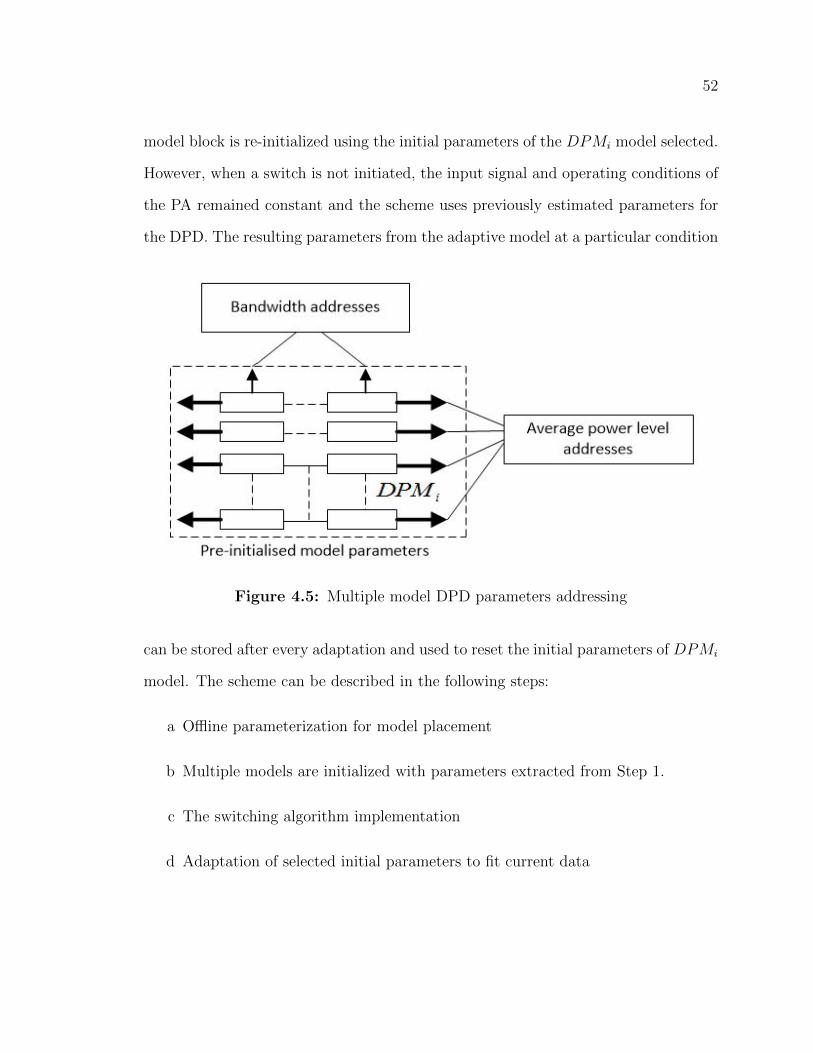
52

model block is re-initialized using the initial parameters of the DPMi model selected.

However, when a switch is not initiated, the input signal and operating conditions of

the PA remained constant and the scheme uses previously estimated parameters for

the DPD. The resulting parameters from the adaptive model at a particular condition

Figure 4.5: Multiple model DPD parameters addressing

can be stored after every adaptation and used to reset the initial parameters of DPMi

model. The scheme can be described in the following steps:

a Offline parameterization for model placement

b Multiple models are initialized with parameters extracted from Step 1.

c The switching algorithm implementation

d Adaptation of selected initial parameters to fit current data

53

4.9.1 Offline Parameterization for Model Placement

The model parameters for each DPD model (DPMi) are initialized at specific values

to minimize transient degradation [41]. The initial values of the model parameters

are determined before the PA startup. Input data, with different statistics, are used

to excite the PA and their corresponding output data are retrieved. A specific input

data and its corresponding output data are referred to as a dataset. The signals used

for initialization are representative of the actual signals to be experienced by the PA

in its real-time operation.

Initial parameters of each model are identified using the procedure similar to the

static DPD synthesis described in Section 4.7. A DPD model, (DPMi), can be defined

by a memory nonlinear polynomial model structure of the form

yi(n) =

Ki∑k=1

Mi−1∑m=0

akmixi(n−m)|xi(n−m)|k−1 (4.24)

where i represents the power level index of a batch of input signals that categorize

an ith operating condition (See Figure 4.6), xi(n) and yi(n) are the input and output

DPD data respectively with unique characteristics, aikm are the model parameters , Ki

is the highest nonlinear order and Mi is the memory length. xi(n), yi(n), aikm , Mi, and

Ki are associated with a DPD model (DPMi). The terms Ki and Mi are real integer

values that determine the configuration of the model structure. The configuration

and structure of each DPMi can be identical or vary across all models. The number

of samples used to estimate the complex-valued parameters, aikm (Equation 4.25), of

each (DPMi), at the ith operating condition must be adequate enough to minimize

54

Figure 4.6: Characteristic plot showing the operation of the PA over i distinctoperating conditions

the cost function E[e2(n)] defined by Equation 4.26.

aikm

T = [ ai10 ai11 ai1M ai20 ai21 ai2M · · · aiK1

aiK2aiKM

] (4.25)

where (.)T is the transpose operator.

E[ei2(n)] =

∑n

(yi(n)− yi(n))2 (4.26)

where yi(n) and yi(n) are the actual output and estimated output respectively asso-

ciated with the ith operating condition modeled by DPMi, and yi(n) is given as

yi(n) = φi(n)akmi(4.27)

and φiT (n) is the regression matrix formulated from the input signal xi(n) associated

55

with the model (DPMi).

φi(n) =

xi10 · · · xi1(M−1) · · · xi11|xi11|K−1 · · · xi1(M−1)|xi1(M−1)|K−1

xi20 · · · xi2(M−1) · · · xi21|xi21|K−1 · · · xi2(M−1)|xi2(M−1)|K−1...

...... · · · ...

......

xiN0 · · · xiN(M−1) · · · xiN1|xiN1|K−1 · · · xiN(M−1)|xiN(M−1)|K−1

(4.28)

The pre-initialised parameters are stored in the memory of the multiple model scheme.

Each set of parameters are addressed based on the statistics of the input signal that

define the PA behavior and operating condition. Figure 4.7 and 4.8 illustrate the

parameter initialization process.

Figure 4.7: DPD scheme parameter initialization

Figure 4.8: Model extraction

56

4.9.2 Hypothesis Test Switching Algorithm

The purpose of multiple model control is to reduce the size of the transient error and

adapt faster to the changes. Therefore, the decision of which model to pick is made

quickly and the selected model should yield the best results when compared to other

models. The purpose is to achieve fast switching by improving convergence to the

new parameter values and accuracy of selection. The DPMi model selected at every

time must give the minimum error E[ei2(n)] between the original input and linearized

output of the PA.

The decision to switch is based on an assertion that the characteristics of the input

signal to the PA, has changed. It is beneficial to make use of inferential statistics which

allows measurement of the properties of the data to detect the changes in the PA.

The hypothesis test based switching algorithm [48] is used to determine changes to

the input signal of the PA. The algorithm ensures data consistency for the case study

presented in this thesis (input power level and bandwidth changes).

The switching algorithm is based on two hypothesis: 1) the null hypothesis Ho

and, 2) the alternative hypothesis Ha. Ho represents a constant PA behavior and

assumes the input data to the PA is not changing. The hypothesis to be proven is

the alternative hypothesis Ha. The purpose of the algorithm is strictly to: Reject the

null hypothesis and accept the alternative if and only if the results of the hypothesis

test are statistically significant.

The hypothesis algorithm can be explained in the following steps:

a State the null hypothesis. In this thesis, the null hypothesis is that the statistics

of the input signal is unchanging.

b Compute the test statistic for statistical significance

c Decision. Accept or reject null hypothesis.

57

The hypothesis is set up as a two-tailed alternative. In the two-tailed test, the result

of the test must be supported by evidence in one of the two directions. Results in

either of the two directions can lead to the rejection of the null nypothesis. When the

alternative hypothesis is accepted, the model with the minimum error is selected.

Test Statistic

The t-test observes the changes in the signal statistics (average power and bandwidth).

The statistics of the pre-processed data signal approximately follows a Gaussian dis-

tribution making the t-test appropriate to monitor statistical changes. The change

in statistics of the signal is observed in the t-test result to(k) which is compared to

a user-defined threshold value Th. The comparison guides the decision of either ac-

cepting or rejecting the null hypothesis. The value of Th corresponds to a significance

level, α, using the statistical t-table.

If N samples (xa(1), xa(2), ..., xa(N)) containing

((Ia(1), Qa(1)), (Ia(2), Qa(2)), ..., (Ia(N), Qa(N))) selected from the current batch a of

input data are compared with another N samples (xb(1), xb(2), ..., xb(N)) containing

((Ib(1), Qb(1)), (Ib(2), Qb(2)), ..., (Ib(N), Qb(N))) selected from the next batch b of

PA input data, the test statistic (t-test) can be defined as

to(k) =

1N

[N∑

n=1

(xa(n)− xb(n))

]S(k)/

√N

(4.29)

where k represents the decision index, and S(k) is the running standard deviation.

xa(n) and xb(n) are absolute values of the signal sequence. The running standard

58

deviation, S(k) is defined as

S(k) =

√√√√ N∑n=1

(xa(n)− xb(n))

N − 1(4.30)

The decision to switch indexed at k is accepted if and only if:

• to(k) ≤ −Th or

• to(k) ≥ +Th

For values of to(k) that lie between −Th and +Th, there is no reason to switch and the

scheme simply maintains the previous model parameters. In the event of a change

in PA characteristics caused by the varying dataset, a switch is permitted to another

model that will yield the least error to ensure model accuracy and maintain the

linearization performance.

Switching Accuracy and Speed

The sample size, N, used in the test statistic computation determines the accuracy

of the hypothesis test. A large sample size increases the accuracy but at the cost

of reduced algorithm speed. A smaller sample size reduces the accuracy of the PA

and increases its speed. The sample size and threshold value are selected to ensure

switches happen when input statistics changes and false switches are not accepted.

The decision to switch is false when the statistics of the input signal and the PA’s

behavior remain unchanged but the test algorithm initiates a switch. In this thesis,

the minimum number of samples that can achieve accuracy and still maintain speed is

determined by a trial and error method. The hypothesis test is a solution to deciding

online the best model to use at a given point in time.

59

4.9.3 Selected Model Adaptation

The DPD model selected at every instant generates the minimum error between

the measured PA input and the linearized PA output. This selection ensures the

linearization performance is maintained. When the switching algorithm is active, a

set of parameters aikm , of a model (DPMi) associated with an ith operating point,

are selected. The selected parameters are used to re-initialize the parameters of the

adaptation model. The adaptive algorithms of Section 3.5.2 initialized using these

parameters are used for adaptation for parameters to re-converge to give the best

possible linearization performance.

Initialization at parameters estimated in advance helps when little is known about

the PA’s operating condition (at start-up and behavior changes). When the power

level of the input signal lies betweem pre-determined ith levels, the statistics of the

data can vary slightly or significantly from the PA data used to estimate the param-

eters for an ith level. However, adaptation from the initialized parameters associated

with any of the adjacent ith levels can help maintain zero control error. The estimated

parameters derived from adaptation are fed into the pre-distorter block continually

to update the DPD parameters. Figure 4.9 illustrates the flowchart for the multiple

model scheme.

The parameters estimated from adaptation for a particular operating condition

can be used to reset the parameters of the fixed DPMi model gotten from the offline

learning. This is the online learning. When an operating condition is experienced

again, the parameters selected for adaptation from the set of DPMi are the ones

learned from adaptation and not the offline-learned parameters.

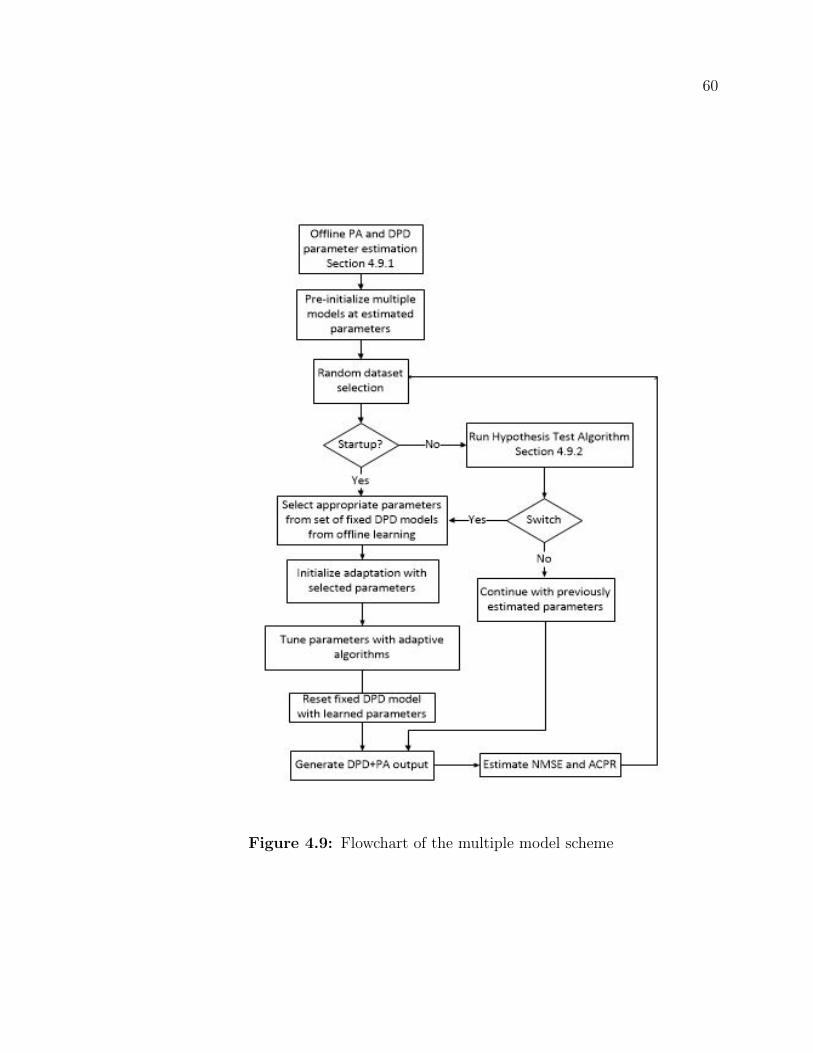
60

Figure 4.9: Flowchart of the multiple model scheme

61

4.10 Multiple Model Configuration

The multiple model digital pre-distorter is more flexible than the single model adap-

tive schemes because each DPD model DPMi can be set to have different model

structures and configurations. A uniform configuration for DPD models with the

same structure means that the nonlinear order Ki and memory depth Mi for each

model are the same. Thus, each model estimate generates an equal number of pa-

rameters.

The total number of parameters to be estimated can be reduced by using different

model configurations for different ith power levels. This is based on the idea that fewer

number of parameters are adequate to model a PA operating at a low power than a

PA at a higher power. Thus, the value of the Ki and Mi set for every power level

is not equal. Moreover, the total number of parameters to be stored in memory and

the overall complexity of the scheme can be significantly reduced during low power

conditions. For all configuration scenerios considered in this thesis, it is assumed that

identical model structures and estimation algorithms are used for all DPD models.

1 Scenario I - Uniform configuration for ith DPD models

• For a multiple model DPD containing DPM1 to DPMi models, the choice

of Ki and Mi for each DPMi are the same. The number of parameters

estimated in each model are equal. i.e.

K1M1 = K2M2 = · · · = KnMn (4.31)

where n is the maximum model number.

2 Scenario II - Non-uniform configuration for ith DPD models

62

• For a multiple model DPD containing DPM1 to DPMi models, the choice

of Ki and Mi for each DPMi are not the sa,e. The number of parameters

estimated in each model DPMi are different from one another. The terms

Ki and Mi can be chosen as

K1M1 ≤ K2M2 ≤ · · · ≤ KnMn (4.32)

such that the sum of all parameters∑i

KiMi < n×KnMn

4.11 Scheme Evaluation

The DPD scheme proposed in this thesis is evaluated based on its linearization per-

formance, the time taken to arrive at acceptable linearization performance (speed)

and the computational complexity.

4.11.1 Linearization Performance

An effective linearization scheme is demonstrated by a significant reduction or com-

plete removal of the in-band distortions and the power interfering in the adjacent

channels otherwise known as the out-of-band emissions seen as spectral regrowth.

The linearization performance of the proposed DPD scheme is evaluated using the

following metrics: 1) the ACPR (frequency domain linearization performance) and

2) the NMSE (time donamin linearization performance).

Digital signal standards such as the 3rd Generation Partnership Project (3GPP)

standard specifies the maximum acceptable ACPR of -45dBc at a 5MHz offset, -50dBc

at a 10MHz offset and the maximum acceptable NMSE value of -35dB for WCDMA

signal formats. [10]. The linearization performance is accepable when the measured

63

ACPR and NMSE are less than the maximum requirements.

The ACPR measures the power in the adjacent channels of the linearized output

as a ratio of the power in its main channel. The frequency domain performance can

also be visualized from the power spectrum density (PSD) plot. The plot shows how

much spectrum regrowth in the linearized output has been suppressed compared to

the original measured output. The PSD in this thesis is estimated using the Welchs

method. The ACPR is calculated as

ACPR = maxm=1,2...

∫(adj)m

|Ylinearized(f)|2df∫ch

|Ylinearized(f)|2df(4.33)

where Ylinearized(f) is the Fourier transform of the DPD+PA output,∫(adj)m

Ylinearized(f)df measures the power in the adjacent channel at m offsets,

and∫

(ch)m

Ylinearized(f)df measures the power in the main channel.

The NMSE compares the input and linearized output in the time domain. The

NMSE evaluates the compensation of in-band distortions (in-band performance) and

the accuracy of the time domain signal after linearization. The NMSE is calculated

as

NMSE(dB) = 10log10

∑n

|x(n)− ylinearized(n)|2∑n

|x(n)|2

(4.34)

Equations 4.33 and 4.34 are similar to the ones previously presented in Section 2.3.2

and 2.3.2 respectively. The previous equations are applied to the measured PA input

and output as opposed to the PA input and linearized PA output (DPD+PA) used

here. The performance of an adaptive DPD scheme is also dependent on the accuracy

of the model estimation. However, the accuracy of the estimated model is dependent

on the model estimation algorithm.

64

4.11.2 Complexity and Speed

Complexity is determined by the amount of mathematical operations that are involved

in achieving the DPD [11, 23]. It is evaluated in terms of the number of additions,

subtractions, divisions, and multiplications required in a computation. In real hard-

ware, complex operations are converted into real operations and memory size has to

be considered. Convergence speed is the time taken for adjusting estimated model

parameters until linearization performance is acceptable.

The speed and complexity of a DPD scheme are interpreted from the number of

samples required to be processed per unit time and the number of parameters to

be estimated. Larger valued parameters require higher resolution digital circuits to

process and store them. An increased number of samples translates to larger matrices

computations which significantly increases complexity.

For accurate model estimation, large sample sizes are required to prevent ill-

conditioned matrices in the estimation. Smaller sample sizes are not fully statistically

representative of the real data and can degrade the linearization performance of the

DPD [55]. A trade-off between the sample size required and degree of estimation

accuracy has to be considered. The smallest sample size possible that can provide an

acceptable degree of accuracy can be selected.

A matrix multiplication AI×JBJ×L will require O⊗AI×JBJ×Lcomplex multiplica-

tions, and O⊕AI×JBJ×Ladditions such that

O⊗AI×J∗BJ×L= J(I × L) (4.35)

O⊕AI×JBJ×L= I × L(J − 1) (4.36)

where A has I rows and J columns, B has J rows and L columns, and the elements of

65

A and B are complex valued. The computation of a matrix inversion CI×I−1, requires

O⊗CI×I−1 multiplications such that

O⊗CI×I−1 = I3 (4.37)

where C has I rows and columns and the elements of C are complex valued. A

complex multiplication is equivalent to four real multiplications [56].

The LS based estimation written as

θK×1 = (φHK×NφN×K)−1φH

K×Ny(n)N×1 (4.38)

where θ represents the parameter vector with K elements, (.)H represents the her-

mitian or complex conjugate transpose, φ(n) represents the regression matrix having

N rows and K columns, and y(n) represents the output data vector of length N ,

requires O⊗LS multiplications and O⊕LS additions where

O⊗LS = N ×K2 × 2 +N ×K +K3 (4.39)

O⊕LS = (N − 1)×K2 +N × (K − 1)×K + (N − 1)×K (4.40)

Computation of the complex-valued parameters per sample using the LMS algo-

rithm O⊗LMS given in Equation 3.15 requires K complex multiplications while the

computation using the RLS estimator O⊗RLS given in Equation 3.19 requires K2

complex multiplications. Thus, the computation complexity per sample for the RLS

is higher than the LMS algorithm. The computation of model parameters with an

identification algorithm using < N samples will be faster than using ≥ N samples.

Likewise, the complexity of the former will be reduced compared to the latter.

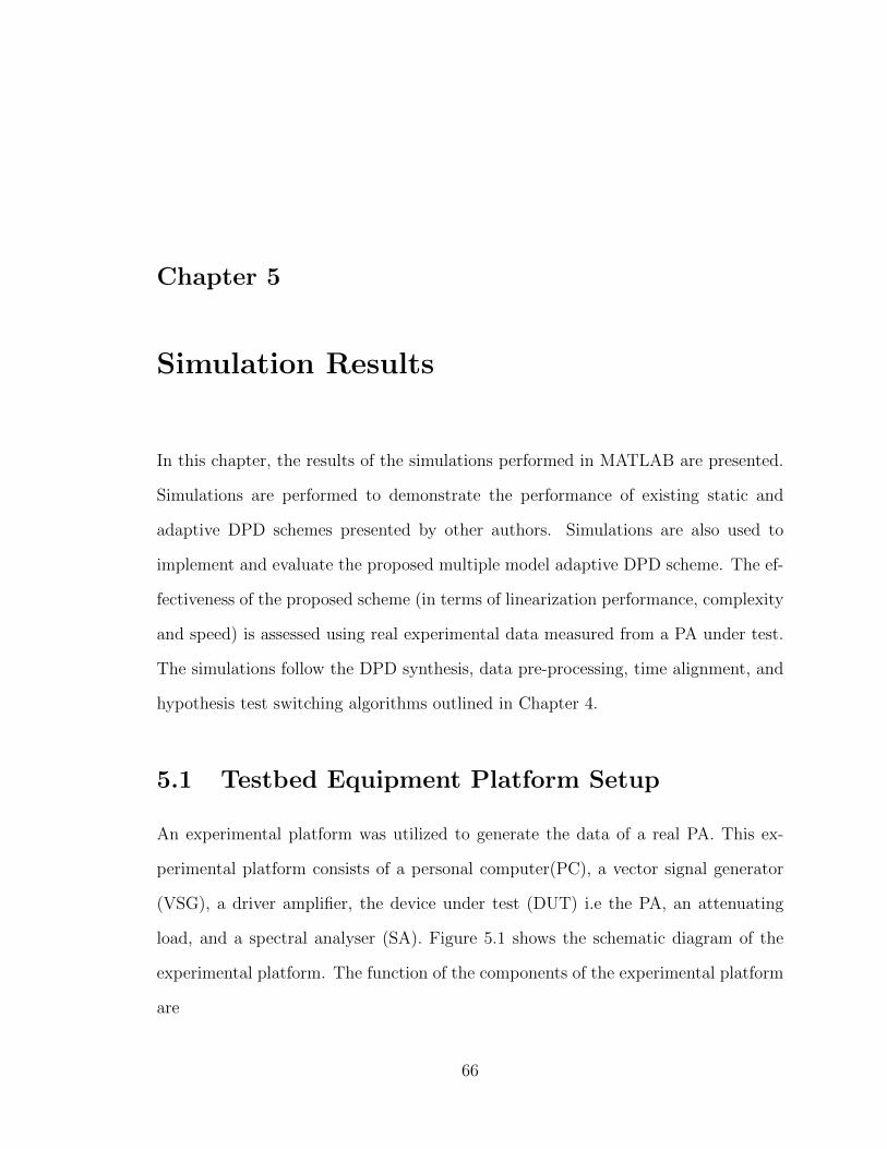
Chapter 5

Simulation Results

In this chapter, the results of the simulations performed in MATLAB are presented.

Simulations are performed to demonstrate the performance of existing static and

adaptive DPD schemes presented by other authors. Simulations are also used to

implement and evaluate the proposed multiple model adaptive DPD scheme. The ef-

fectiveness of the proposed scheme (in terms of linearization performance, complexity

and speed) is assessed using real experimental data measured from a PA under test.

The simulations follow the DPD synthesis, data pre-processing, time alignment, and

hypothesis test switching algorithms outlined in Chapter 4.

5.1 Testbed Equipment Platform Setup

An experimental platform was utilized to generate the data of a real PA. This ex-

perimental platform consists of a personal computer(PC), a vector signal generator

(VSG), a driver amplifier, the device under test (DUT) i.e the PA, an attenuating

load, and a spectral analyser (SA). Figure 5.1 shows the schematic diagram of the

experimental platform. The function of the components of the experimental platform

are

66

67

Figure 5.1: Block diagram of the experimental platform setup

• A - The PC running MATLAB simulation software. It generates complex

baseband PA input excitation signals and uploads the data to the vector signal

generator. The output data sequence is downloaded to the PC with a spectrum

analyser (SA) data acquisition software.

• B - The Agilent E4438C ESG Vector signal generator (VSG) with 250kHz -

6GHz instantaneous bandwidth. The VSG converts the digital input signal fed

from the PC to analog signals and up-converts the PA input to a bandpass

signal. The signal generated from the VSG is fed to a linear driver amplifier.

• C - The driver amplifier is fed with the up-converted analog signal from the

VSG before it is sent to the Phoenix PA1109C DUT. The pre-amplifier prepares

the signal for further processing by the PA.

• D - The DUT is a Phoenix PA1109C 10VDC PA operating at a frequency

range of 1.8 - 2GHz. The PA is supplied by a DC power source of 12V. The

1dB compression point at the input of the PA is 33dB.

• E - A 6dB RF attenuator is placed at the DUT’s output. The output signal is

then connected to the spectrum analyser.

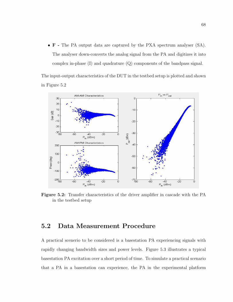
68

• F - The PA output data are captured by the PXA spectrum analyser (SA).

The analyser down-converts the analog signal from the PA and digitizes it into

complex in-phase (I) and quadrature (Q) components of the bandpass signal.

The input-output characteristics of the DUT in the testbed setup is plotted and shown

in Figure 5.2

Figure 5.2: Transfer characteristics of the driver amplifier in cascade with the PAin the testbed setup

5.2 Data Measurement Procedure

A practical scenerio to be considered is a basestation PA experiencing signals with

rapidly changing bandwidth sizes and power levels. Figure 5.3 illustrates a typical

basestation PA excitation over a short period of time. To simulate a practical scenario

that a PA in a basestation can experience, the PA in the experimental platform

69

Figure 5.3: Changing input signals experienced by a PA over time

explained in the previous section, is excited by multicarrier WCDMA baseband signals

with varying bandwidth and power levels. The input signals are:

• complex two-carrier (2C) WCDMA with a PAPR of 7.49dB and total bandwidth

of 10-MHz sampled at 100Mbps.

• complex four-carrier (4C) WCDMA signals (1111 carrier configuration - all car-

riers are used) with a PAPR of 7.64dB and total bandwidth of 20-MHz sampled

at 100Mbps.

The amplitude setting of the input signal in the VSG is varied (reference power level)

to drive the PA over a large dynamic range (linear and nonlinear modes). The input

signal set at different ith (high and low) average power levels is used to drive the

PA. In order to protect the amplifier and the system from overheating, the maximum

peak amplitude of the input signal at both bandwidths is limited to -10.5dBm. A

million I/Q input data samples are uploaded and the corresponding output data are

downloaded.

70

The datasets (input and corresponding output at an ith power level) are grouped

and labelled for simplicity. Table 5.1 is a list of all the datasets measured at specific

ith power levels used in simulations. The ith input amplitude setting is the power

level of the input signal adjusted at the ESG Vector signal generator shown in Figure

5.1. The output power is the measured average power level of the output signals

downloaded from the PC.

Figure 5.4 shows the power spectrum density (PSD) plots of the two- and four-

carrier WCDMA input and output datasets at different power levels. The legends

in the plots correspond to the dataset, amplitude settings and carrier type listed in

Table 5.1 The lowest traces in Figures 5.4(a) and 5.4(b) are the input signals with

over 60dB dynamic range. The output traces show the spectral regrowth caused

by the amplifier, which is as high as -25dB. The output traces are the plots of the

original measured output signals shifted by a scaling factor defined in Section 4.5

(small signal gain). This is done to align the output trace with the input signal

trace for convenience in displaying PSD plots. The output plots of all other figures

hereafter shown in this chapter are shifted for convenience in displaying results.

71

Table 5.1: List of measured input and output multicarrier signals at different ithpower levels. The label i is the index of the input signal’s power level thatspecifies the ith operating condition. The label (Di) represents the index of thedataset (input and corresponding output) with a carrier size and at a specificith power level setting

Dataset (Di) Test signal type ith Input Output Power (dBm)amplitude setting (dBm)

1 2C-WCDMA -10.5 -25.31

2 2C-WCDMA -11.5 -25.98

3 2C-WCDMA -12.5 -26.69

4 2C-WCDMA -13.5 -27.44

5 2C-WCDMA -14.5 -28.33

6 2C-WCDMA -15.5 -29.26

7 2C-WCDMA -16.5 -30.17

8 2C-WCDMA -17.5 31.13

9 2C-WCDMA -18.5 -32.12

10 4C-WCDMA -10.5 -25.37

11 4C-WCDMA -11.5 -26.01

12 4C-WCDMA -12.5 -26.72

13 4C-WCDMA -13.5 -27.51

14 4C-WCDMA -14.5 -28.38

15 4C-WCDMA -15.5 -29.29

16 4C-WCDMA -16.5 -30.22

17 4C-WCDMA -17.5 -31.19

18 4C-WCDMA -18.5 -32.17

19 4C-WCDMA -19.5 -33.17

72

(a)

(b)

Figure 5.4: PSD plots of measured input and output (a) two-carrier WCDMAand (b) four-carrier WCDMA signals for various amplitude settings (legendscorrespond to ith values in Table 5.1)

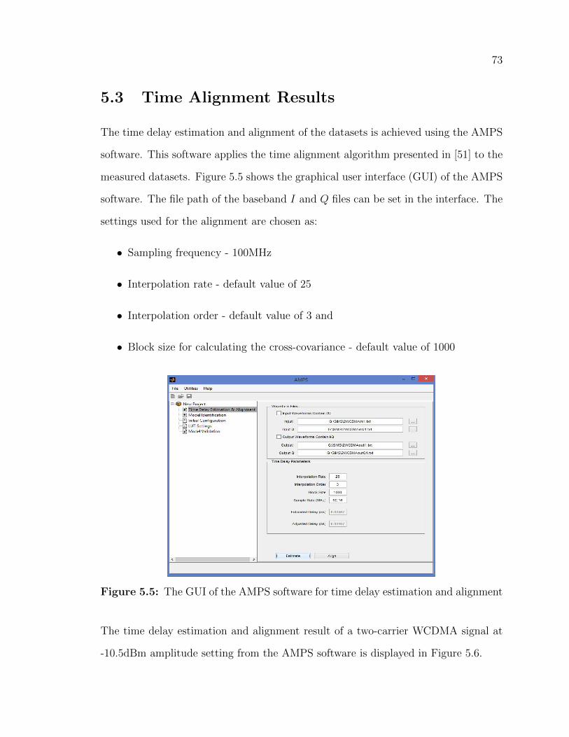
73

5.3 Time Alignment Results

The time delay estimation and alignment of the datasets is achieved using the AMPS

software. This software applies the time alignment algorithm presented in [51] to the

measured datasets. Figure 5.5 shows the graphical user interface (GUI) of the AMPS

software. The file path of the baseband I and Q files can be set in the interface. The

settings used for the alignment are chosen as:

• Sampling frequency - 100MHz

• Interpolation rate - default value of 25

• Interpolation order - default value of 3 and

• Block size for calculating the cross-covariance - default value of 1000

Figure 5.5: The GUI of the AMPS software for time delay estimation and alignment

The time delay estimation and alignment result of a two-carrier WCDMA signal at

-10.5dBm amplitude setting from the AMPS software is displayed in Figure 5.6.

74

Figure 5.6: Comparison between the time domain plot of (a) the original measuredinput and the aligned input (b) the original measured output and the alignedoutput and (c) the aligned input and the output signal of a 2C-WCDMA signal

5.4 PA Characterization

The input and output signals measured are used to construct the AM/AM and

AM/PM responses of the PA at any ith operating condition. Figure 5.7 and 5.8

show the AM/AM and AM/PM characteristic plots of the PA for the two- and four-

carrier WCDMA datasets with different bandwidths and input power levels. The

AM/AM and AM/PM plots for different datasets show the dependence of the PA’s

operating point on the statistics (bandwidth and power level) of the input signal.

The increased dispersions observed in the characteristic plot for the 4C-WCDMA

signal compared to that of the 2C-WCDMA shows the increase in memory effect on

the PA as a result of an increase in the bandwidth of the signal. The plots for high

(-10.5dBm) and low (-18.5dBm) power levels show the increase in the severity of the

PA’s nonlinearity as the input power level increases. This confirms the idea that the

PA behavior is different for different input signals.

75

(a) (b)

Figure 5.7: AM/AM and AM/PM response when the PA is excited by a two-carrierWCDMA signal at an input power level of (a) -10.5dBm and (b) -18.5dBm

(a) (b)

Figure 5.8: AM/AM and AM/PM response when the PA is excited by a four-carrierWCDMA signal at an input power level of (a) -10.5dBm and (b) -18.5dBm

The ACPR for the original input and output signals measured are computed. The

adjacent channel offsets of a WCDMA signal are typically 5MHz, 10MHz, and 15MHz

from the carrier. Offsets are measured from the first carrier for lower adjacent channel

and the last carrier for the upper adjacent channel. The ACPR of the input signal at

a particular bandwidth is constant for all power levels. The worst case ACPR in the

+5MHz or −5MHz channel offset of the output signal is considered for evaluating the

linearization performance. Table 5.2 lists the ACPR (±5MHz offset) calculated for

76

the input and output datasets measured from the PA before linearization (without

a DPD). The measured output signal does not have equal ACPR at ±5MHz offset

Table 5.2: ACPR values of measured datasets for simulation

Dataset No.Input ACPR (dBc) Output ACPR (dBc)

±5MHz -5MHz +5MHz1 -62.82 -36.07 -35.482 -62.82 -38.01 -37.453 -62.82 -40.20 -39.694 -62.82 -42.79 -42.275 -62.82 -46.18 -45.786 -62.82 -49.35 -49.227 -62.82 -52.38 -52.338 -62.82 -54.75 -54.749 -62.82 -56.33 -55.8010 -53.77 -24.25 -23.0611 -53.77 -26.00 -25.0012 -53.77 -28.15 -27.2813 -53.77 -30.82 -30.0814 -53.77 -34.00 -33.5115 -53.77 -37.42 -37.1716 -53.77 -40.88 -40.7317 -53.77 -44.13 -44.0818 -53.77 -46.65 -46.5719 -53.77 -48.51 -48.40

as observed from the asymmetrical output spectrum plot of Figure 5.4 which further

confirms that a PA with memory nonlinearity generates an asymmetrical output

spectrum plot.

5.5 Static DPD Simulation

The performance of a static DPD using the particular datasets measured is evaluated.

The results from the static DPD simulation is used to:

77

• Verify the effect of the nonlinear and memory order of a model structure on the

modeling accuracy, and the DPD performance.

• Compare the linearization performance of signals at the same power levels and

modulation but different bandwidth.

• Compare the linearization performance for signals with same modulation, same

bandwidth but different power levels.

• Study the poor linearization performance of a static DPD for a PA experiencing

rapid signal changes.

5.5.1 PA and DPD Modeling Simulation

The accuracy of the PA and DPD model is evaluated using the NMSE between the

estimated model output from simulation, and the original measured input. An unbi-

ased estimate of the PA and DPD will proportionally improve the overall linearization

performance. The modeling accuracy of an estimation at a particular configuration

can be affected by the:

• varying bandwidth sizes of signals at a fixed power level and

• varying power levels of signals at fixed bandwidth

The choice of the model configuration also has a significant effect on the modeling

accuracy of an estimation.

1 Fixed Power Level, Varying Bandwidth and Model Configurations

Different configurations (polynomial order K and memory depth order M) of the

memory polynomial model, for the PA and DPD estimation, are tested. We use

1000 samples to extract the parameters of the PA and DPD model for different

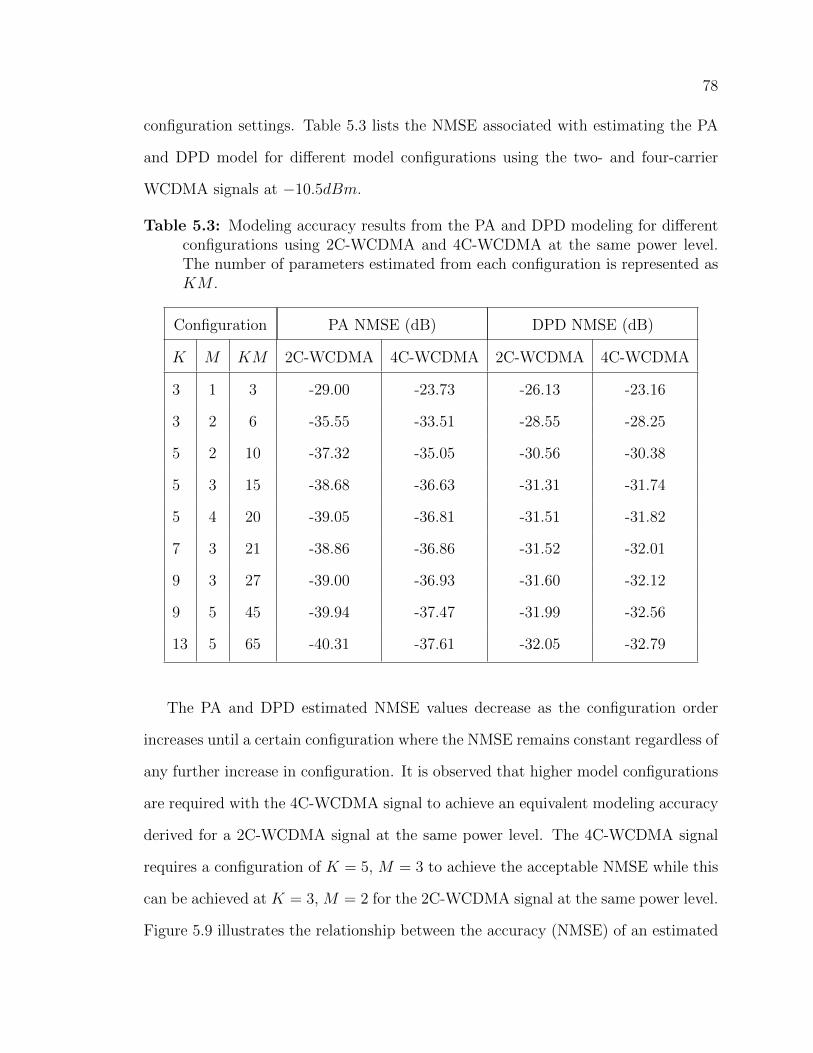
78

configuration settings. Table 5.3 lists the NMSE associated with estimating the PA

and DPD model for different model configurations using the two- and four-carrier

WCDMA signals at −10.5dBm.

Table 5.3: Modeling accuracy results from the PA and DPD modeling for differentconfigurations using 2C-WCDMA and 4C-WCDMA at the same power level.The number of parameters estimated from each configuration is represented asKM .

Configuration PA NMSE (dB) DPD NMSE (dB)

K M KM 2C-WCDMA 4C-WCDMA 2C-WCDMA 4C-WCDMA

3 1 3 -29.00 -23.73 -26.13 -23.16

3 2 6 -35.55 -33.51 -28.55 -28.25

5 2 10 -37.32 -35.05 -30.56 -30.38

5 3 15 -38.68 -36.63 -31.31 -31.74

5 4 20 -39.05 -36.81 -31.51 -31.82

7 3 21 -38.86 -36.86 -31.52 -32.01

9 3 27 -39.00 -36.93 -31.60 -32.12

9 5 45 -39.94 -37.47 -31.99 -32.56

13 5 65 -40.31 -37.61 -32.05 -32.79

The PA and DPD estimated NMSE values decrease as the configuration order

increases until a certain configuration where the NMSE remains constant regardless of

any further increase in configuration. It is observed that higher model configurations

are required with the 4C-WCDMA signal to achieve an equivalent modeling accuracy

derived for a 2C-WCDMA signal at the same power level. The 4C-WCDMA signal

requires a configuration of K = 5, M = 3 to achieve the acceptable NMSE while this

can be achieved at K = 3, M = 2 for the 2C-WCDMA signal at the same power level.

Figure 5.9 illustrates the relationship between the accuracy (NMSE) of an estimated

79

model and the number of estimated model parameters.

Figure 5.9: NMSE values compared to the number of parameters used to model aPA and DPD for a two-carrier(blue) and a four-carrier (red) WCDMA signalat an ith power level

2 Varying Power Level, Fixed Bandwidth and Model Configuration

Modeling of the PA and DPD with high powered signals require higher model con-

figurations than with low powered signals. An increase in the configuration settings

does not guarantee an improvement in the linearization performance and modeling

accuracy. This is because a certain configuration is adequate to capture the nonlinear

and memory effects of the PA for the highest powered signal that can excite a PA.

Table 5.4 shows the accuracy of the models estimated for the two-carrier WCDMA

signal at different power levels using a fixed model configuration of K = 5 and M = 3.

The NMSE value reduces as the power level of the signal reduces for modeling with

the same configuration. The nonlinear order of a model for estimating the behavior of

a PA and DPD increases with the power level of the dataset until acceptable accuracy

80

Table 5.4: Comparison of the PA and DPD modeling accuracy with a fixed config-uration for the 2C-WCDMA signal at different power levels

Dataset PA NMSE (dB) DPD NMSE (dB)

2C-WCDMA @ -10.5dBm -38.68 -31.312C-WCDMA @ -11.5dBm -41.53 -35.082C-WCDMA @ -12.5dBm -43.63 -38.962C-WCDMA @ -13.5dBm -45.17 -42.572C-WCDMA @ -14.5dBm -46.04 -44.892C-WCDMA @ -15.5dBm -45.74 -44.962C-WCDMA @ -16.5dBm -46.02 -45.22

is achieved. The memory depth order required for a model also increases with the

bandwidth of the dataset.

The computational complexity for estimating the model increases with an increase

in the configuration order because of the increase in the number of parameters to be

estimated. Therefore, a trade-off between accuracy and complexity has to made. The

least configuration possible to achieve the acceptable performance is usually a good

choice if complexity of implementation is of high importance.

5.5.2 Static DPD Linearization Performance

The static DPD is simulated using the procedure outlined in Chapter 4 and its lin-

earization performance is evaluated. The case of a PA experiencing input signal

changes is considered to study the poor performance of a static DPD (Figure 5.10).

At a time t, the PA is excited by a -10.5dBm 4C-WCDMA signal. The DPD at this

time t is modeled using 1000 data samples from the 4C-WCDMA dataset. Figure

5.11(a) shows the PSD plots of the original input, original output without DPD and

the output after the static DPD is applied to a PA excited by a 4C-WCDMA sig-

nal at a specific time t. The output spectrum regrowth shown as the red trace was

significantly suppressed by about 25dB to give the green trace in Figure 5.11(a).

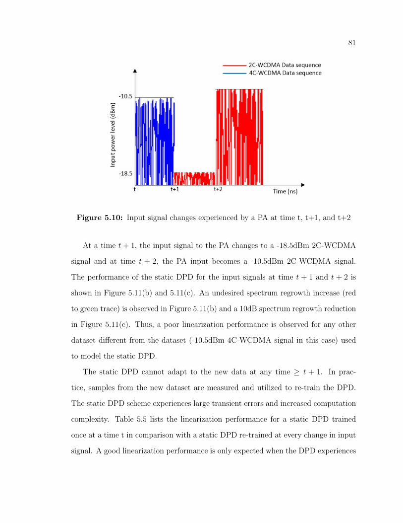
81

Figure 5.10: Input signal changes experienced by a PA at time t, t+1, and t+2

At a time t + 1, the input signal to the PA changes to a -18.5dBm 2C-WCDMA

signal and at time t + 2, the PA input becomes a -10.5dBm 2C-WCDMA signal.

The performance of the static DPD for the input signals at time t + 1 and t + 2 is

shown in Figure 5.11(b) and 5.11(c). An undesired spectrum regrowth increase (red

to green trace) is observed in Figure 5.11(b) and a 10dB spectrum regrowth reduction

in Figure 5.11(c). Thus, a poor linearization performance is observed for any other

dataset different from the dataset (-10.5dBm 4C-WCDMA signal in this case) used

to model the static DPD.

The static DPD cannot adapt to the new data at any time ≥ t + 1. In prac-

tice, samples from the new dataset are measured and utilized to re-train the DPD.

The static DPD scheme experiences large transient errors and increased computation

complexity. Table 5.5 lists the linearization performance for a static DPD trained

once at a time t in comparison with a static DPD re-trained at every change in input

signal. A good linearization performance is only expected when the DPD experiences

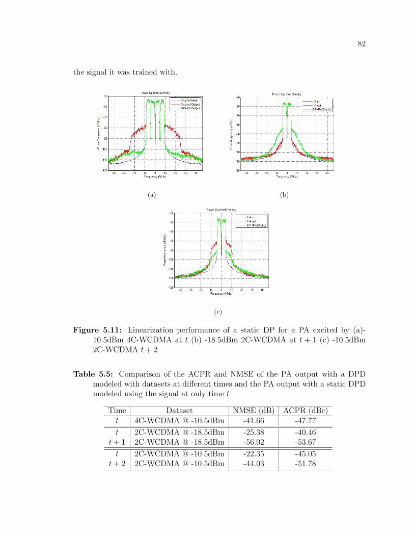
82

the signal it was trained with.

(a) (b)

(c)

Figure 5.11: Linearization performance of a static DP for a PA excited by (a)-10.5dBm 4C-WCDMA at t (b) -18.5dBm 2C-WCDMA at t + 1 (c) -10.5dBm2C-WCDMA t+ 2

Table 5.5: Comparison of the ACPR and NMSE of the PA output with a DPDmodeled with datasets at different times and the PA output with a static DPDmodeled using the signal at only time t

Time Dataset NMSE (dB) ACPR (dBc)t 4C-WCDMA @ -10.5dBm -41.66 -47.77

t 2C-WCDMA @ -18.5dBm -25.38 -40.46t+ 1 2C-WCDMA @ -18.5dBm -56.02 -53.67

t 2C-WCDMA @ -10.5dBm -22.35 -45.05t+ 2 2C-WCDMA @ -10.5dBm -44.03 -51.78

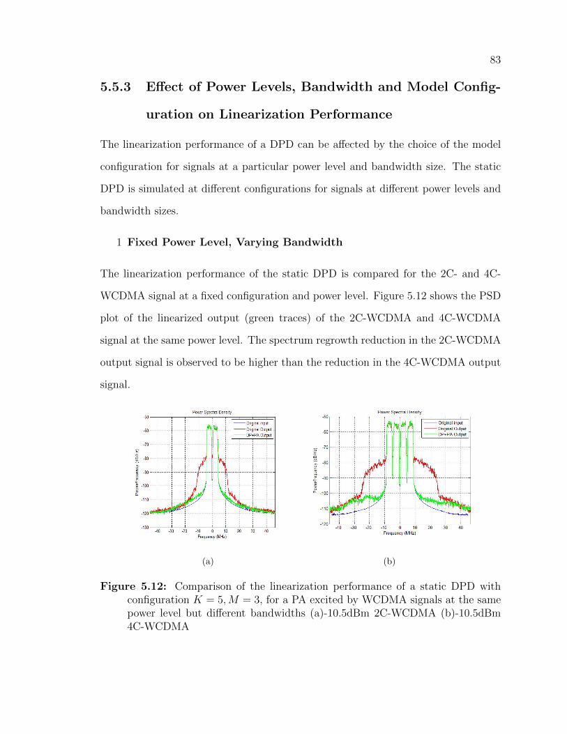
83

5.5.3 Effect of Power Levels, Bandwidth and Model Config-

uration on Linearization Performance

The linearization performance of a DPD can be affected by the choice of the model

configuration for signals at a particular power level and bandwidth size. The static

DPD is simulated at different configurations for signals at different power levels and

bandwidth sizes.

1 Fixed Power Level, Varying Bandwidth

The linearization performance of the static DPD is compared for the 2C- and 4C-

WCDMA signal at a fixed configuration and power level. Figure 5.12 shows the PSD

plot of the linearized output (green traces) of the 2C-WCDMA and 4C-WCDMA

signal at the same power level. The spectrum regrowth reduction in the 2C-WCDMA

output signal is observed to be higher than the reduction in the 4C-WCDMA output

signal.

(a) (b)

Figure 5.12: Comparison of the linearization performance of a static DPD withconfiguration K = 5,M = 3, for a PA excited by WCDMA signals at the samepower level but different bandwidths (a)-10.5dBm 2C-WCDMA (b)-10.5dBm4C-WCDMA

84

The linearization performance of the static DPD is also compared at different

configurations for the 2C-WCDMA and 4C-WCDMA signals at the same power level.

Table 5.6 shows the ACPR and NMSE achieved for the 4C-WCDMA signal and 2C-

WCDMA signal at a fixed power level for different configurations. At a given power

level, higher configuration orders are required for signals at a higher bandwidth to

give comparable linearization performances when signals at a lower bandwidth are

used.

Table 5.6: Linearization performance for varying model configurations using the2C-WCDMA and 4C-WCDMA signal at -10.5dBm

Model configuration Dataset NMSE(dB) ACPR (dBc)K = 3 2C-WCDMA -27.34 -36.96M = 2 4C-WCDMA -27.14 -31.89K = 5 2C-WCDMA -44.03 -51.78M = 3 4C-WCDMA -41.66 -47.23K = 7 2C-WCDMA -44.68 -52.33M = 3 4C-WCDMA -42.02 -47.77

2 Varying Power Levels, Fixed Bandwidth

The linearization performance of the static DPD is compared at different configura-

tions for the 2C-WCDMA or 4C-WCDMA signal for different power levels. Table

5.7 shows that the linearization performance increases as the model configuration is

increased for a high powered signal. A poor performance of -31.89dBc (above -45dBc

threshold) was observed for the -10.5dBm 4C-WCDMA signal with a model configu-

ration of K = 3,M = 2. At low order model configurations, the DPD is inadequate

to successfully suppress the spectrum outgrowth for high powered signals. The PSD

plots of the DPD+PA output for different model configurations for a high and low

powered 2C-WCDMA and 4C-WCDMA signal is shown in Figures 5.13 and 5.14.

85

Table 5.7: Linearization performance (ACPR in dBc) for different configurationsusing the 4C-WCDMA signal at varying power levels

Dataset K = 3, M = 2 K = 5, M = 3 K = 7, M = 3

4C-WCDMA @ -10.5dBm -31.89 -47.77 -47.234C-WCDMA @ -11.5dBm -35.81 -50.83 -50.504C-WCDMA @ -12.5dBm -40.13 -52.20 -52.614C-WCDMA @ -13.5dBm -45.16 -52.43 -53.234C-WCDMA @ -14.5dBm -50.01 -52.94 -53.43

(a) (b)Figure 5.13: Comparison of the linearization performance of a static DPD with

configuration K = 3,M = 2 and K = 5,M = 3, at -10.5dBm (high poweredsignal) for (a) a 2C-WCDMA signal and (b) a 4C-WCDMA signal

(a) (b)Figure 5.14: Comparison of the linearization performance of a static DPD with

configuration K = 3,M = 2 and K = 5,M = 3, at -17.5dBm (low poweredsignal) for (a) a 2C-WCDMA signal and (b) a 4C-WCDMA signal

86

Acceptable performance is only achieved when the configuration increases for high

powered signals. However, at this same configuration, the DPD using 4C-WCDMA

signals with power levels lesser than -12.5dBm (lower powered signals) can achieve

good performance. Thus, low order DPD model configurations are adequate for the

PA excited by low powered signals.

5.6 First Order Linear Digital Pre-distortion

Following from the results presented in Section 5.5 and shown in Figure 5.14, the

PA behavior is close to linear for input signals at low power levels. A PA exhibiting

mild nonlinearity can be linearized by a simple first order linear model-based DPD.

A simple first order linear function is used as the PA and DPD model. The measured

AM/AM and AM/PM characteristics of the PA are fitted to a linear first order model.

The parameters of the model and its inverse are estimated using adaptive algorithms

outlined in Chapter 3. Figure 5.15 is a block diagram of a 1st order linear model

based pre-distorter.

Figure 5.15: Block diagram of a first order linear adaptive DPD

87

It is assumed that the PA behavior follows a 1st order linear transfer function:

YPA(z)

XPA(z)=

bz

z − a(5.1)

where YPA(z) and XPA(z) are the output and input of the PA respectively and the

parameters of the model are the terms a and b. Equation 5.1 can be re-written as

yPA(n) = ayPA(n− 1) + bxPA(n) (5.2)

The PA’s inverse function for the DPD is

YDP (z)

XDP (z)=z − abz

(5.3)

where YDP (z) and XDP (z) are the output and input of the DPD respectively. Equa-

tion 5.3 can also be re-written as

yDP (n) =1

bxDP (n)− a

bxDP (n− 1) (5.4)

Figures 5.16(a) and 5.16(b) are time plots of the original output and estimated output

for the PA and DPD modeling using a first order linear function. The high modeling

accuracy is observed from the plot as the estimated output approximately equal to the

original measured output. Table 5.8 lists the NMSE and ACPR of low powered 2C-

and 4C-WCDMA signals using the first order adaptive DPD. The very low values of

the ACPR and NMSE in the table indicates the high linearization performance that

can be achieved with the first order linear model-based adaptive DPD scheme.

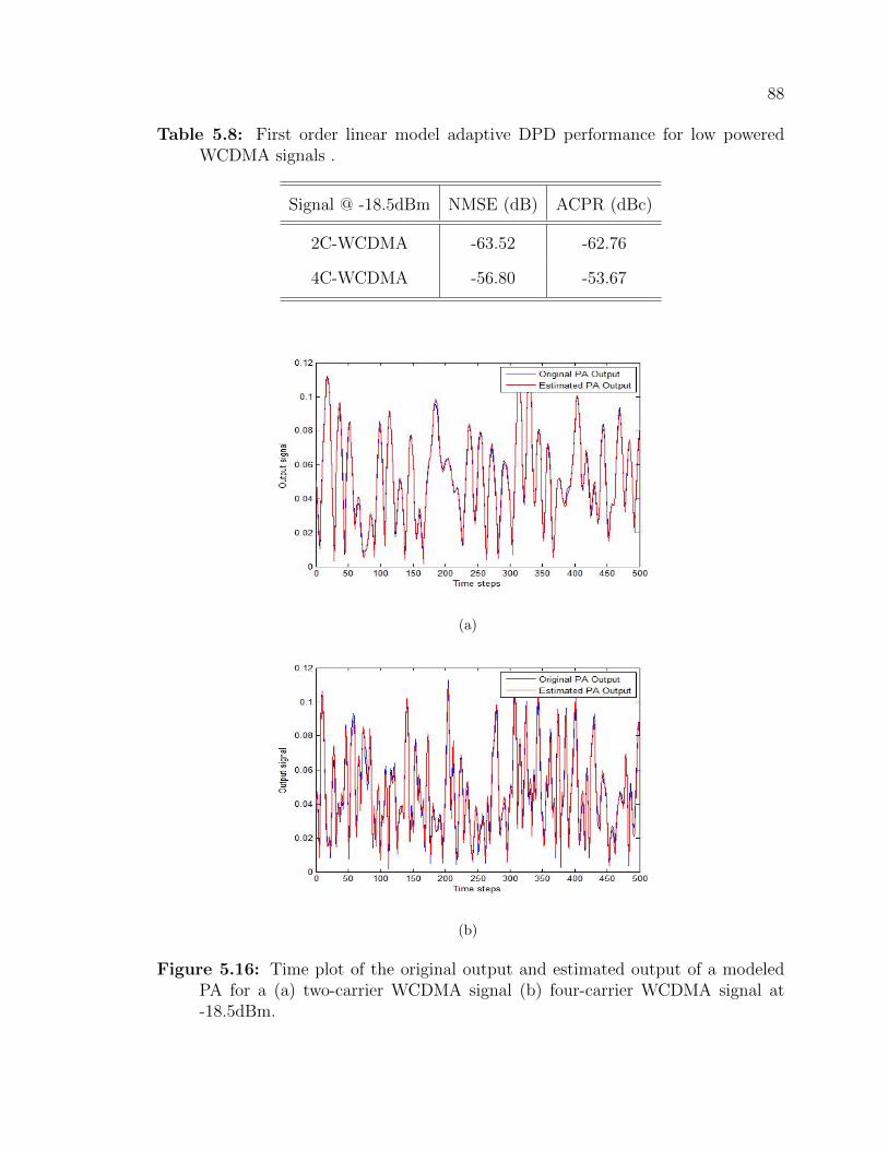
88

Table 5.8: First order linear model adaptive DPD performance for low poweredWCDMA signals .

Signal @ -18.5dBm NMSE (dB) ACPR (dBc)

2C-WCDMA -63.52 -62.76

4C-WCDMA -56.80 -53.67

(a)

(b)

Figure 5.16: Time plot of the original output and estimated output of a modeledPA for a (a) two-carrier WCDMA signal (b) four-carrier WCDMA signal at-18.5dBm.

89

The cascade of the first order DPD and PA is the original signal at the PA’s

input. Figure 5.17 shows the performance of a PA linearized with a first order linear

model ADPD. The DPD is capable of reproducing the original PA input without any

observable spectrum regrowth. Also, the first order linear model ADPD requires the

estimation of only two parameters and provides a good linearization of the PA at low

operating power condition at a relatively fast speed.

(a)

(b)

Figure 5.17: PSD plots of the original input, the original output before the DPDand the simulated DPD+PA output of a low powered (a) two-carrier WCDMAsignal and (b) four-carrier WCDMA signal using the first order linear model-based ADPD

90

The implementation of the first order linear DPD is simpler and less complex than

a nonlinear model DPD that can require estimation of more than two parameters.

However, the first order model is not sufficient to compensate for the increased non-

linearity exhibited by the PA at a higher operating power level. Figure 5.18 shows the

minimal spectral regrowth reduction for output signal for a PA at a high operating

power condition.

Figure 5.18: PSD plots showing linearization performance of the first order linearmodel ADPD for a high powered 4C-WCDMA signal.

5.7 Memory Polynomial Based Adaptive DPD

Simulation

An adaptive DPD is simulated for the same scenerio presented in Section 5.5.2. The

algorithm of this DPD requires a fixed model configuration setting for different input

signals. The model configuration chosen should be able to compensate for the non-

linearity imposed on the most complex signal (signal with highest power level and

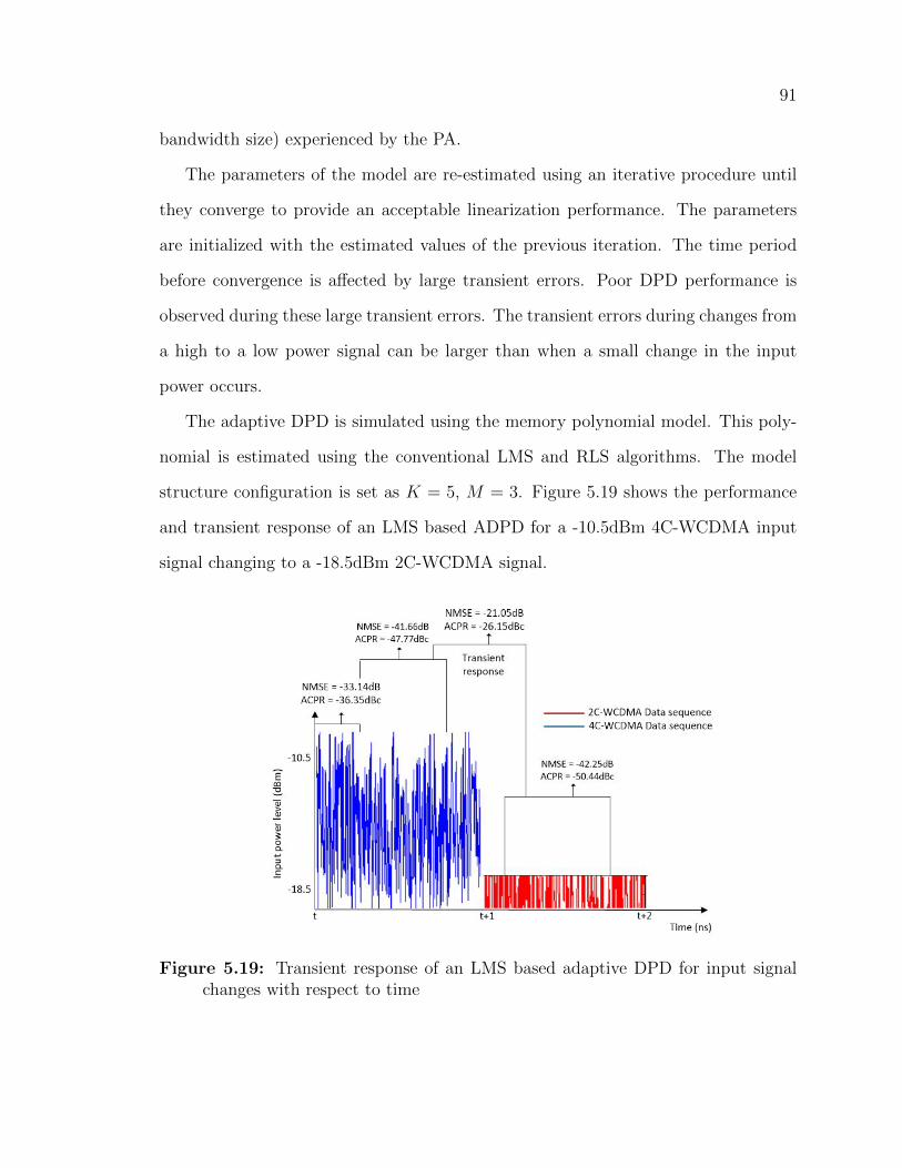
91

bandwidth size) experienced by the PA.

The parameters of the model are re-estimated using an iterative procedure until

they converge to provide an acceptable linearization performance. The parameters

are initialized with the estimated values of the previous iteration. The time period

before convergence is affected by large transient errors. Poor DPD performance is

observed during these large transient errors. The transient errors during changes from

a high to a low power signal can be larger than when a small change in the input

power occurs.

The adaptive DPD is simulated using the memory polynomial model. This poly-

nomial is estimated using the conventional LMS and RLS algorithms. The model

structure configuration is set as K = 5, M = 3. Figure 5.19 shows the performance

and transient response of an LMS based ADPD for a -10.5dBm 4C-WCDMA input

signal changing to a -18.5dBm 2C-WCDMA signal.

Figure 5.19: Transient response of an LMS based adaptive DPD for input signalchanges with respect to time

92

The results of the NMSE and ACPR show that degradation of the DPD perfor-

mance occurs at the time when the input signal changes. The linearization perfor-

mance cannot be maintained at acceptable values at such times. The parameters of

the DPD change and only re-converge to accurately compensate for the PA distortions

after an adequate number of iterations have occured from a window containing only

samples from the current dataset. Considering the sequence of the datasets studied,

the LMS based adaptive DPD required about 50,000 samples from the current dataset

to achieve acceptable linearization performance. The RLS based adaptive DPD re-

quired about 500 samples. Table 5.9 summarizes the linearization performance of the

LMS and RLS based adaptation for input signal changes of samples taken from a

clear set of a particular data.

Table 5.9: Comparison of the linearization performance (NMSE & ACPR) betweenthe LMS (> 50,000 samples) and RLS ( > 500 samples) based adaptive DPD

.

Dataset sequenceNMSE (dB) ACPR (dBc)

LMS RLS LMS RLS

4C-WCDMA @ -10.5dBm -32.82 -39.99 -36.49 -45.45

2C-WCDMA @ -17.5dBm -36.21 -56.40 -49.72 -60.02

2C-WCDMA @ -10.5dBm -31.21 -43.21 -42.77 -52.38

2C-WCDMA @ -11.5dBm -32.88 -42.96 -43.32 -51.14

4C-WCDMA @ -18.5dBm -40.35 -55.17 -48.56 -53.55

2C-WCDMA @ -15.5dBm -47.71 -59.52 -58.72 -62.11

2C-WCDMA @ -15.5dBm -47.71 -59.52 -58.72 -62.11

2C-WCDMA @ -14.5dBm -36.85 -54.06 -55.45 -60.87

2C-WCDMA @ -10.5dBm -30.98 -42.94 -42.09 -51.55

4C-WCDMA @ -10.5dBm -26.99 -35.68 -35.40 -40.85

93

The sequence of signal changes follows a pre-determined pattern that is repre-

sentative of rapid signal variations in practice. Figure 5.20 shows the PSD plot of

the linearization performance for an LMS and RLS based adaptive scheme for 500

samples of the two- and four-carrier WCDMA signal.

(a)

(b)

Figure 5.20: PSD plots of the original input, the original output before DPD, thesimulated LMS based DPD+PA output and the simulated RLS based DPD+PAoutput with 1000 samples from a pure batch of high powered (a) two-carrierWCDMA signal (b) four-carrier WCDMA signal

94

The result demonstrate a distortion correction of about 20dB and 7dB for the RLS

based ADPD and LMS based ADPD respectively. An adaptive DPD with the RLS

algorithm compensates for the distortions faster than one with the LMS algorithm.

The batch of samples utilized to test the DPD is different from the batch of samples

utilized to train the adaptive DPD.

5.8 Multiple Model Switching Algorithm

The linearization performance of the multiple model (MM) scheme depends on the

ability of the switching algorithm to identify changes in datasets quickly and accu-

rately. In the multiple model simulation, offline learning of the model parameters for

different datasets is done to initialize the fixed DPMi models, the hypothesis algo-

rithm is implemented to decide switching, and the DPD model parameters associated

with the particular operating condition is selected and used to initialize the adaptive

model. The adaptive model ADPM tunes the parameters to fit the particular dataset

and can be used to reset the fixed DPMi models. The order of changes in the PA

excitation signal is determined before simulation to enable examination of

• changes in signal power levels at a constant bandwidth

• changes in signal power levels with varying bandwidth

• changes in bandwidth sizes at a constant power level

• constant excitation signals

The hypothesis test based switching algorithm is applied to the input and output

datasets to determine bandwidth changes and power level changes respectively. The

double check ensures that wrong decisions to switch are avoided as a switch is initiated

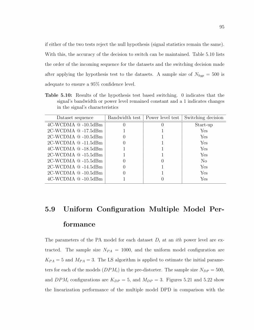
95

if either of the two tests reject the null hypothesis (signal statistics remain the same).

With this, the accuracy of the decision to switch can be maintained. Table 5.10 lists

the order of the incoming sequence for the datasets and the switching decision made

after applying the hypothesis test to the datasets. A sample size of Nhyp = 500 is

adequate to ensure a 95% confidence level.

Table 5.10: Results of the hypothesis test based switching. 0 indicates that thesignal’s bandwidth or power level remained constant and a 1 indicates changesin the signal’s characteristics

Dataset sequence Bandwidth test Power level test Switching decision

4C-WCDMA @ -10.5dBm 0 0 Start-up2C-WCDMA @ -17.5dBm 1 1 Yes2C-WCDMA @ -10.5dBm 0 1 Yes2C-WCDMA @ -11.5dBm 0 1 Yes4C-WCDMA @ -18.5dBm 1 1 Yes2C-WCDMA @ -15.5dBm 1 1 Yes2C-WCDMA @ -15.5dBm 0 0 No2C-WCDMA @ -14.5dBm 0 1 Yes2C-WCDMA @ -10.5dBm 0 1 Yes4C-WCDMA @ -10.5dBm 1 0 Yes

5.9 Uniform Configuration Multiple Model Per-

formance

The parameters of the PA model for each dataset Di at an ith power level are ex-

tracted. The sample size NPA = 1000, and the uniform model configuration are

KPA = 5 and MPA = 3. The LS algorithm is applied to estimate the initial parame-

ters for each of the models (DPMi) in the pre-distorter. The sample size NDP = 500,

and DPMi configurations are KDP = 5, and MDP = 3. Figures 5.21 and 5.22 show

the linearization performance of the multiple model DPD in comparison with the

96

LMS based adaptive DPD for low and high powered signals.

(a)

(b)

Figure 5.21: Comparison of the linearization performance of the multiple modeland LMS based ADPD for low powered (a) two-carrier WCDMA signal and (b)four-carrier WCDMA signal.

When switching is initiated because of a signal change, a set of fixed parameters

learned offline and stored in memory that can maintain acceptable performance is

selected. The adaptive model block is initialized at the selected parameters chosen

from the fixed DPMi model. The parameters re-converge to fit the particular datasets

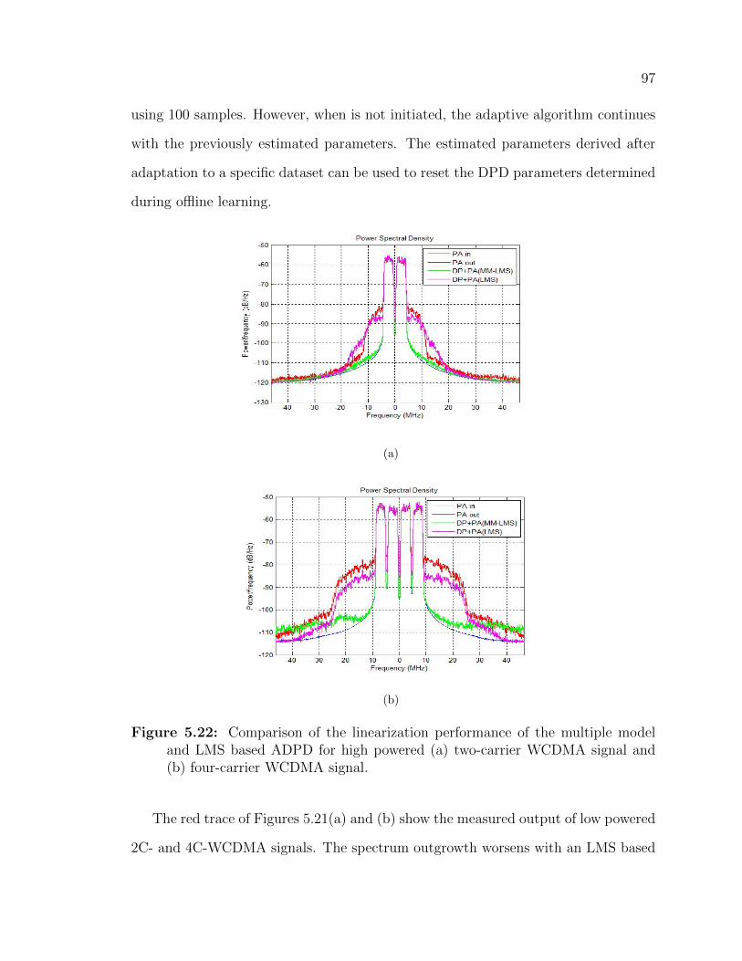
97

using 100 samples. However, when is not initiated, the adaptive algorithm continues

with the previously estimated parameters. The estimated parameters derived after

adaptation to a specific dataset can be used to reset the DPD parameters determined

during offline learning.

(a)

(b)

Figure 5.22: Comparison of the linearization performance of the multiple modeland LMS based ADPD for high powered (a) two-carrier WCDMA signal and(b) four-carrier WCDMA signal.

The red trace of Figures 5.21(a) and (b) show the measured output of low powered

2C- and 4C-WCDMA signals. The spectrum outgrowth worsens with an LMS based

98

ADPD (pink trace) compared to the distortion reduction provided by the multiple

model scheme (green trace). The spectrum regrowth cannot be reduced with the

LMS based ADPD and is observed to worsen in the case of low powered signals. The

distortion reduction of the LMS based ADPD for high powered signals is significantly

far lesser than that of the proposed scheme as shown in Figures 5.22(a) and (b). The

results indicate that the MM scheme achieves and maintains acceptable linearization

performance for input signal changes at different power levels.

The linearization performance of the RLS based ADPD is also compared to the

MM scheme. As demonstrated from the results of Section 5.7, the RLS based ADPD

can achieve acceptable performance with 500 samples from a window of a particular

dataset at an ith power level. However, it is not certain that the performance can be

maintained for all signal changes. This is demonstrated to be true from the NMSE and

ACPR results for the RLS based ADPD and MM scheme using the LMS algorithm

(MM-LMS) listed in Table 5.10. The RLS based ADPD is not guaranteed to maintain

Table 5.11: Comparison of the linearization performance (NMSE & ACPR) of theRLS based ADPD and the multiple model scheme at varying signal changes

Dataset selected Algorithms ACPR (dBc) NMSE(dB)

2C-WCDMA @ -17.5dBmWithout DPD -54.75 -

RLS -60.89 -51.49MM-LMS -62.73 -61.48

2C-WCDMA @ -10.5dBmWithout DPD -36.07 -

RLS -48.90 -35.78MM-LMS -51.05 -38.50

4C-WCDMA @ -18.5dBmWithout DPD -46.57 -

RLS -52.13 -50.03MM-LMS -53.51 -55.03

4C-WCDMA @ -10.5dBmWithout DPD -23.06 -

RLS -39.84 -32.76MM-LMS -46.43 -35.69

99

the performance for all signal changes. The ACPR and NMSE values are shown to

increase significantly above the -45dBc and -35dB constraints respectively with the

RLS based ADPD for a -18.5dBm 4C-WCDMA signal changing to a -10.5dBm 4C-

WCDMA signal. The MM-LMS is seen to maintain linearization performance at the

time of this change.

Furthermore, the linearization performance of the proposed multiple model ap-

proach is assessed in comparison with the RLS based ADPD and LMS based ADPD

Figures 5.23 and 5.24 show the PSD plots for the output signal: without a DPD,

with the RLS based ADPD, with the LMS based ADPD, and the proposed multiple

model scheme The plots show that the proposed scheme gives the highest spectral

reduction (green traces) followed by the black traces representing the output spectra

for the RLS based ADPD. The LMS based ADPD gives the least spectral reduction

as shown by the pink traces.

5.10 Discussion

Overall, the results of Section 5.9 are discussed here.

I Linearization Performance Results

The simulation results of Section 5.9 show that the LMS based ADPD gives a poor

performance that violates the constraints on the ACPR and NMSE values as the PA

excitation signal changes. The linearization performance deteriorates at the point

of a sudden change and a good linearization performance can only be guaranteed

after 50000 samples from a window containing only samples from a particular dataset

have been processed. In other words, more than 50000 samples have to be processed

before acceptable requirements are met. In a situation where 50000 samples from a

100

(a)

(b)

Figure 5.23: Measured PA output spectra showing: the measured input (blue),measured output without a DPD (red), output with the LMS based adaptivepre-distorter (pink), RLS based adaptive pre-distorter (black), and LMS basedmultiple model (green) for signal change to (a) -17.5dBm two-carrier WCDMAsignal, (b) -17.5dBm four-carrier WCDMA signal.

101

(a)

(b)

Figure 5.24: Measured PA output spectra showing: the measured input (blue),measured output without a DPD (red), output with the LMS based adaptiveADPD (pink), RLS based adaptive ADPD (black), and proposed multiple modelscheme (green) for (a) -10.5dBm two-carrier WCDMA signal, (b) -10.5dBmfour-carrier WCDMA signal.

102

particular dataset at ith power level cannot be processed because signals change even

more rapidly, the DPD performance degrades even more and becomes unstable.

The plots show that the RLS based ADPD with 500 samples can achieve compa-

rable performance as the proposed scheme. However, this level of performance cannot

be maintained when signals switch from a high powered signal to a low powered sig-

nal. When a signal switches from a high power (-10.5dBm 2C-WCDMA signal) to

a low power (-18.5dBm 4C-WCDMA signal ) as shown in Table 5.11, the DPD has

been trained to compensate for the PA over the entire dynamic range and can still

work properly with the PA excited by the lower signal. For a low to a high power

signal switch, the parameters of the DPD are not sufficient to compensate for the

higher nonlinearity experienced. A switch from the -18.5dBm 4C-WCDMA signal to

the -10.5dBm 4C-WCDMA in Table 5.11 shows the deterioration in the performance

of the RLS based ADPD.

The MM scheme proposed maintains linearization performance for all switching

possiblities. This is as a result of the offline-learned parameters used to initialize the

adaptation for signal changes. The hypothesis test based switching technique can

accurately deal with the problem of switching with 500 samples. This makes it faster

and more suitable for use in a rapidly changing PA input signal scenerio.

II Complexity and Speed

The LMS based ADPD computation per sample requires K × M complex multi-

plications which is equal to 4 × K × M real multiplications. The computation of

the LMS based ADPD goes through 50000 samples to achieve acceptable perfor-

mance. Thus, 4× 50000×{K ×M}2 real multiplications is required for every signal

change. However, the RLS based ADPD attaining good performance with 500 sam-

ples will be computed using 500 × {K ×M}2 complex multiplication equivalent to

4× 500× {K ×M}2 real multiplications.

103

The hypothesis test algorithm in the MM scheme involves no matrix inversions

or complex multiplications. The computation involves additions, subtractions and

divisions operating on 500 samples to monitor signal changes. The adaptation of

parameters to new values requires 100 samples during signal changes. Computation

will require 4×100×{K ×M} real multiplications. The memory storage for the initial

parameters estimated is not considered. It is assumed that this will have little or no

significant effect on the computational complexity. The one-time offline computation

of the initial parameters is also not considered.

The comparison of the number of samples and computations required by each

scheme indicates that the MM scheme offers a faster adaptation with reduced com-

plexity compared to other schemes discussed here.

5.11 Non-uniform Configuration Multiple Model

Performance

The sets of models in the multiple model DPD scheme can be configured with different

nonlinear and memory orders depending on the power level of the input signal. The

results in Section 5.5 have shown that low DPD model configurations are adequate

when the PA experiences low powered signals while high powered signals require

higher configurations. The non-uniform configuration multiple model scheme uses

this idea to reduce the number of parameters to be estimated and the computation

complexity associated with the estimation when signal changes to a low powered

signal. Table 5.12 shows the choice of configurations for the particular datasets used

in this thesis. At initialization, the number of parameters to be estimated is reduced.

Table 5.13 shows the parameter savings at initialization for the non-uniform multiple

104

Table 5.12: Choice of model configuration settings chosen for different power levelranges

Dataset (Dr) Power level range Model configuration2C-WCDMA

-10.5dBm to -14.5dBm K = 5, M = 34C-WCDMA

2C-WCDMA-15.5dBm to -19.5dBm K = 3, M = 2

4C-WCDMA

model configuration compared to the uniform configuration. When the input signal

changes from a high powered to a low powered signal, the number of parameters

to be estimated is reduced from 15 to 6. Figure 5.25 shows the performance of

Table 5.13: Parameter savings estimation

Configuration Power levels Parameters/model Models TotalUniform 15 19 285

Non-uniformHigh 6 9

54 + 150 = 204Low 15 10

Parameter savings 81

the non-uniform configuration multiple model scheme using K = 3, M = 2 for

a low powered signal PA excitation compared to the performance of the uniform

configuration that requires K = 5, M = 3 for the same low powered signal. the plots

show that the spectrum regrowth seen in the red trace representing the output without

DPD is reduced to the same level by both configurations For the datasets used, the

performance of the multiple model scheme with a configuration of K = 5, M = 3 for

high powered signals is compared to a configuration of K = 7, M = 5. Figure 5.26

shows the comparable performance achieved using a multiple model configuration of

K = 5, M = 3 and K = 7, M = 5.

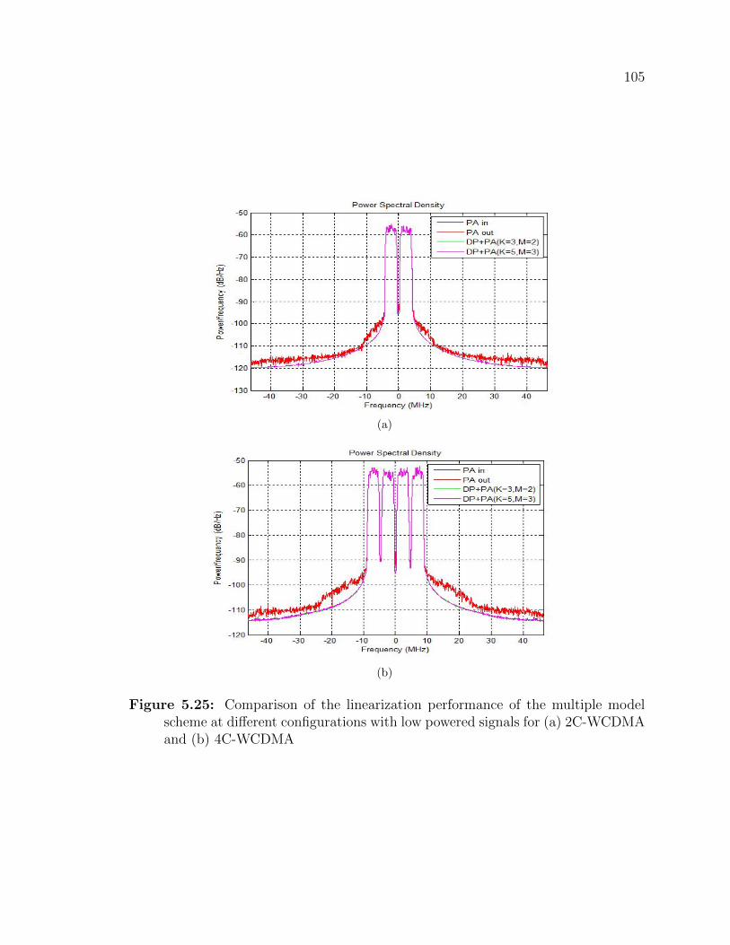
105

(a)

(b)

Figure 5.25: Comparison of the linearization performance of the multiple modelscheme at different configurations with low powered signals for (a) 2C-WCDMAand (b) 4C-WCDMA

106

(a)

(b)

Figure 5.26: Comparison of the linearization performance of the multiple modelscheme at different configurations with high powered signals for (a) 2C-WCDMA and (b) 4C-WCDMA

It is observed that the model configuration of K = 5, M = 3 is adequate for the

highest power signal measured from the PA. A higher configuration of K = 7, M = 5

will only increase the computation complexity without an associated improvement in

the linearization performance.

107

5.12 Discussion

The non-uniform configuration multiple model scheme is shown to further reduce the

computation complexity and increase speed of the proposed DPD scheme. The offline

estimation of initial parameters provides an opportunity to understand the PA before

it is set to operate in the basestation. The test signals at varying power levels used

for initialization are similar to the ones to be experienced in practice. The highest

nonlinearity of the PA can be studied and the appropriate model configuration for

each operating condition of the PA can be decided beforehand. The benefit of this

is a faster adaptation when any slight reduction in the number of parameters to be

estimated significantly improves the speed of the DPD.

5.13 Online Adaptive Parameter Learning

The re-converged parameters estimated after a switch has been initiated due to a

signal change can be used to reset the offline estimated parameters of the fixed DPMi

models of the multiple model scheme. This describes the online learning adaptive

portion for the proposed scheme. At a time t when the PA is excited by a signal

xa(n), the chosen fixed parameters learned offline serve as a strategic initialization

point for adaptation.

When the excitation signal changes at a time t+1 to xb(n), the adaptation is re-

initialized with the parameters of the appropriate model related to the power level of

xb(n). The resulting parameters after every adaptation for xa(n) and xb(n) are used

to reset the fixed parameters learned offline associated with the power level of the

signal. At any other time t+q when either xa(n) or xb(n) re-excite the PA, the learned

parameters stored are selected. The excitation of the PA by re-occurring signals will

require little or no adaptation with this resetting capability of the adaptive model in

108

the proposed scheme.

Adaptation from the online learned parameters only provides slight improvement

to the linearization performance and it is can be possible to cut-off the adaptive

scheme after all possible operating conditions of the PA have been learned over time.

Table 5.14 shows the linearization performance for the first and subsequent occur-

rences of the 2C- and 4C-WCDMA signal as the PA excitation signal at different

times. It may be true with the data used for simulation that after learning has oc-

Table 5.14: NMSE and ACPR for 2C- and 4C-WCDMA signals exciting the PA attime t (first occurrence) and at time t+q (subsequent occurence) when offlineor online learned parameters are used

Time ParametersSignal

2C-WCDMA 4C-WCDMANMSE (dB) ACPR (dBc) NMSE (dB) ACPR(dBc)

t Offline -38.50 -51.05 -35.69 -46.43

t+qOffline -38.50 -51.05 -35.69 -46.43Online -39.57 -51.08 -36.71 -46.47

cured for all operating conditions, no further changes happen to the parameters and

consequently no further improvement in the linearization performance. Therefore,

adaptation may seem no longer necessary as the PA model is only described at these

levels. However, it is worth noting that factors affecting the operating conditions of

the PA can also be long-term [42] and different from the short-term factors (varying

input signal characteristics) considered in this work.

The consideration of other factors beyond the scope of the work in this thesis that

can still affect the linearization performance of the DPD is an important issue in a

real DPD deployment. In such cases, adaptation from learned parameters will remain

necessary and desired. A more advanced learning module will be to store parameters

into newly generated DPMi models for different operating conditions encountered

during the course of learning.

109

5.14 Number of Models Reduction

This thesis focused on the impact of varying input signals on the PA behavior. The

plots of the input and output signals extracted from a PA at different power levels

confirm that the PA behavior for each dataset at a particular bandwidth size and

power level is different. A certain dataset cannot be used to model the PA for the full

dynamic range of operation of the PA. In turn, the DP exhibits different character-

istics with respect to different operating conditions of the PA. In simulation, unique

parameters of the PA model are estimated for each dataset to be used in the multiple

model scheme.

In order to reduce the number of models in the multiple model scheme, the power

range of low powered signals can be increased. In this thesis, three low powered

datasets at -17.5dBm to -19.5dBm are combined to represent all signals at a power

level <-17.5dBm. The parameters of each model at these power levels can be com-

bined through coefficient averaging to give only one set of model parameters.

The first order linear model can also be used in place of low configuration MP

models for low powered input signals. Further reduction of complexity and improved

speed can be gained by incorporating the simpler linear model at low power level

ranges. However, the smaller ranges considered for high powered signals is still re-

quired because nonlinear behavior varies significantly from one another with small

power variations for high powered signals.

5.15 Summary

This chapter presented the simulation results from the test and validation of the

proposed multiple model scheme. Real data signals of a PA were obtained from an

110

experimental platform and utilized to model the digital pre-distorter using the MAT-

LAB simulation tool. The PA linearisation performance, complexity and response

time of the digital pre-distorter was studied using input signals with different band-

width sizes. The simulation results of the static and adaptive pre-distorter schemes

was used for comparison with the proposed scheme to demonstrate its effectiveness.

It was observed that the LMS based ADPD offered large transient errors and

instability in performance. The RLS based ADPD offered faster convergence of DPD

parameters but at the cost of high computation complexity. The multiple model

scheme was shown to offer faster adaptation to maintain the linearization performance

for all possible signal changes with reduced computation complexity. The hypothesis

test based switching incorporated with the proposed scheme used 500 samples for

very fast switching.

Chapter 6

Conclusion and Future Work

6.1 Conclusion

The work presented in this thesis establishes the importance of an adaptive DPD

scheme as a solution to rapidly changing PA behavior caused by the variations in the

input excitation signals. A static DPD designed to compensate for the nonlinearity

at the operating condition of a PA can adequately linearize the PA. The current

operating condition is defined by the input signal at a particular power level and

bandwidth. However, the performance of the DPD at all other times when input

signal changes have occurred is undesirable.

The static DPD scheme is also associated with significantly high computation

complexity. A new batch of samples from the current dataset have to be collected

and the parameters re-estimated. Thus, they can only be desired for PAs that are not

expected to change behaviors over a long period of time. For such PAs, it is assumed

that the input signals do not change and only slow-varying long-term factors such as

temperature can affect the PA during its operation.

Adaptive DPD schemes offer real time online compensation that can continu-

ously adapt to the PA’s changing behavior. However, one major problem with the

111

112

conventional schemes is that the linearization performance cannot be maintained at

acceptable values. The estimators used in the adaptive schemes have computational

complexity problems. Rapid fluctuations in power levels and bandwidth sizes de-

grade the PA performance and the adaptive DPD requires more time to track the

rapid fluctuations that may result in relatively large transient errors.

Furthermore, adaptive schemes require the use of a single fixed model and con-

figuration for estimating the parameters of the DPD. The configuration is set to suit

the most complex signal to be experienced by the PA and this remains constant

for all power levels and bandwidth sizes of the input signal. Therefore, the same

number of parameters are required to be estimated for all power levels. Low power

operating conditions that can be sufficiently represented with fewer parameters are

overparameterized.

The multiple model adaptive DPD is explored in this work as a solution to in-

crease convergence speed and reduce computation complexity of achieving digital

pre-distortion. The structure of the multiple model scheme consists of a hybrid of

the static and adaptive estimators, and it incorporates the hypothesis switching al-

gorithm to accurately decide when to switch. To demonstrate the viability of the

multiple model scheme with a real PA, real WCDMA test signals were used in simu-

lations.

Simulations showed that the multiple model adaptive DPD scheme was able to

maintain the linearization performance at an acceptable value for all possible in-

put signal variations defined by standard set NMSE and ACPR thresholds. The

scheme also offered faster adaptation in terms of the number of signals required to

be processed per signal change. The RLS based adaptive DPD offered relatively fast

re-convergence speed at signal changes. However, the RLS based ADPD cannot main-

tain a good performance for all situations. Furthermore, the multiple model scheme

113

offered reduced computation complexity than the RLS based ADPD.

In general, the multiple model scheme yielded lower transient error response than

the conventional adaptive schemes. In comparison with other existing work that

propose variants of the conventional adaptive schemes, the proposed scheme was

simulated/demonstrated for a PA operating over a wide dynamic range within a very

short period of time. In addition, the reduced cost implication of the proposed scheme

is highly significant. The reduced computation complexity means reduced resources

in hardware implementations. Linearization for low powered signals can be achieved

using fewer parameters derived from estimation.

Part of the work done in this thesis also investigated the need for using different

sets of parameters to model the PA for signals at different power levels. From sim-

ulations, it was seen that a set of parameters cannot be used to represent the PA

behavior in its full dynamic range. Although a wide range in low operating power

conditions can be represented with a set of model parameters, the same cannot be

applied when the PA is operating at higher nonlinear modes. Moreover, the PA be-

havior of adjacent higher power operating regions are significantly different from each

other.

6.2 Future Work

The work presented in this thesis provides potential directions for future research. The

viability of the proposed scheme demonstrated through simulation can be extended

by implementing the scheme in real hardware to test the performance and validate

the idea proposed in the scheme.

One of the advantages of the multiple model scheme is the flexibility in the choice

of the model structure, configuration, and estimation algorithm for the set of models

114

used in the DPD. The set-up used in this thesis explored using only non-uniform

configurations in the models. Hence, more work to explore the possibilities of using

varying model structures and estimation algorithms can be done. Studying the effect

of these other possibilities on the overall performance of the DPD will be an interesting

area to investigate.

The PA in the equipment testbed platform for acquiring measurement data used

in this work exhibits weak nonlinearity that can sufficiently be modeled with 15

parameters. Current PAs have severely high nonlinearities that would require more

than fifteen parameters to generate an unbiased estimate of the PA and in effect,

improve the efficiency of the DPD.

The power levels and amplitude settings considered in this work were non-

overlapping. It would be an area of interest to explore results for overlapping power

level ranges and power levels that fall in between the ones considered in this work.

Moreover, the reduction of the number of models required in the DPD, explored by

increasing the range for the amplitude setting and power levels of the input signal,

can also be considered at overlapping levels.

The adaptive learning component of the proposed scheme can further be re-

searched to improve the effectiveness and reduce the overall complexity of the pro-

posed scheme. Low powered signals can be modeled with a fixed set of parameters

that will not be reset by the adaptive scheme. The adaptive learning component can

be designed to function only with the higher power level signals that require more

adaptation to achieve better linearization performance.

References

[1] F. Mkadem, Behavioural Modeling and Linearization of RF Power Amplifier

using Artificial Neural Networks. PhD thesis, University of Waterloo, May 2010.

[2] Chih-Hung Lin, Hsin-Hung Chen, Yung-Yi Wang, and Jiunn-Tsair Chen, “Dy-

namically optimum lookup-table spacing for power amplifier predistortion lin-

earization,” IEEE Transactions on Microwave Theory and Techniques, vol. 54,

pp. 2118–2127, May 2006.

[3] A. Wright and W. Durtler, “Experimental performance of an adaptive digital

linearized power amplifier (for cellular telephony),” IEEE Transactions on Ve-

hicular Technology, vol. 41, no. 4, pp. 395–400, 1992.

[4] X. Yu, Contributions to Digital Predistortion of Radio-Frequency Power Ampli-

fiers for Wireless Applications. PhD thesis, Contributions to Digital Predistor-

tion of Radio-Frequency Power Amplifiers for Wireless Applications, 2012.

[5] O. Andersen, P. Malmlof, and D. Wisell, “Nonlinear Characterization of Multiple

Carrier Power Amplifiers,” in 56th ARFTG Conference Digest, vol. 38, pp. 1–8,

IEEE, Nov. 2000.

[6] F. Luo, Digital Front-End in Wireless Communications and Broadcasting: Cir-

cuits and Signal Processing. Cambridge University Press, 2011.

[7] A. S. Tehrani, T. Eriksson, and C. Fager, “Modeling of long term memory ef-

fects in RF power amplifiers with dynamic parameters,” in 2012 IEEE/MTT-S

International Microwave Symposium Digest, pp. 1–3, IEEE, June 2012.

[8] F. Ghannouchi and O. Hammi, “Behavioral modeling and predistortion,” IEEE

Microwave Magazine, vol. 10, pp. 52–64, Dec. 2009.

[9] S. Andreoli, H. McClure, P. Banelli, and S. Cacopardi, “Digital linearizer for RF

amplifiers,” IEEE Transactions on Broadcasting, vol. 43, pp. 12–19, Mar. 1997.

115

116

[10] C. Potter, “System analysis of a W-CDMA base-station PA employing adap-

tive digital predistortion,” IEEE Radio Frequency Integrated Circuits (RFIC)

Symposium., 2002.

[11] A. D’Andrea, V. Lottici, and R. Reggiannini, “A digital approach to efficient RF

power amplifier linearization,” in GLOBECOM 97. IEEE Global Telecommuni-

cations Conference. Conference Record, vol. 1, pp. 77–81, IEEE, 1997.

[12] S. A. Bassam, M. Helaoui, and F. M. Ghannouchi, “2-D Digital Predistortion

(2-D-DPD) Architecture for Concurrent Dual-Band Transmitters,” IEEE Trans-

actions on Microwave Theory and Techniques, vol. 59, pp. 2547–2553, Oct. 2011.

[13] D. Morgan, Z. Ma, J. Kim, M. Zierdt, and J. Pastalan, “A Generalized Mem-

ory Polynomial Model for Digital Predistortion of RF Power Amplifiers,” IEEE

Transactions on Signal Processing, vol. 54, pp. 3852–3860, Oct. 2006.

[14] L. Ding, G. Zhou, D. Morgan, Z. Ma, J. Kenney, J. Kim, and C. Giardina, “A

Robust Digital Baseband Predistorter Constructed Using Memory Polynomials,”

IEEE Transactions on Communications, vol. 52, pp. 159–165, Jan. 2004.

[15] J. Kim and K. Konstantinou, “Digital predistortion of wideband signals based

on power amplifier model with memory,” Electronics Letters, vol. 37, no. 23,

p. 1417, 2001.

[16] O. Ata, “Predistort-linearisation method for future basestation amplifiers of cel-

lular radio,” in Proceedings of PIMRC ’96 - 7th International Symposium on

Personal, Indoor, and Mobile Communications, vol. 2, pp. 267–271, IEEE, 1996.

[17] J. Cavers, “Amplifier linearization using a digital predistorter with fast adapta-

tion and low memory requirements,” IEEE Transactions on Vehicular Technol-

ogy, vol. 39, no. 4, pp. 374–382, 1990.

[18] S. Boumaiza and F. M. Ghannouchi, “Realistic power-amplifiers characterization

with application to baseband digital predistortion for 3G base stations,” IEEE

Transactions on Microwave Theory and Techniques, vol. 50, pp. 3016–3021, Dec.

2002.

[19] K. Lee and P. Gardner, “Comparison of different adaptation algorithms for adap-

tive digital predistortion based on EDGE standard,” in 2001 IEEE MTT-S In-

ternational Microwave Sympsoium Digest, vol. 2, pp. 1353–1356, IEEE, 2001.

117

[20] T. Fujinaka and S. Omatu, “A switching scheme for adaptive control using multi-

ple models,” in IEEE SMC’99 Conference Proceedings. 1999 IEEE International

Conference on Systems, Man, and Cybernetics (Cat. No.99CH37028), vol. 5,

pp. 80–85, IEEE, 1999.

[21] Y. Nagata, “Linear amplification technique for digital mobile communications,”

in IEEE 39th Vehicular Technology Conference, pp. 159–164, IEEE, 1989.

[22] D. M. Giesbers, Adaptive digital polynomial predistortion linearisation for RF

power amplifiers. PhD thesis, University of Canterbury, 2008.

[23] A. D’Andrea, V. Lottici, and R. Reggiannini, “RF power amplifier linearization

through amplitude and phase predistortion,” IEEE Transactions on Communi-

cations, vol. 44, no. 11, pp. 1477–1484, 1996.

[24] S. C. Cripps, Advanced Techniques in RF Power Amplifier Design. Artech House,

2002.

[25] S. Boumaiza, T. Liu, and F. Ghannouchi, “On the Wireless Transmitters Linear

and Nonlionear Distortions Detection and Pre-Correction,” in 2006 Canadian

Conference on Electrical and Computer Engineering, pp. 1510–1513, IEEE, 2006.

[26] D. Wisell, “A baseband time domain measurement system for dynamic charac-

terization of power amplifiers with high dynamic range over large bandwidths,”

in Proceedings of the 20th IEEE Instrumentation Technology Conference, vol. 2,

pp. 1177–1180, IEEE, 2003.

[27] K. M. Gharaibeh, Nonlinear Distortion in Wireless Systems: Modeling and Sim-

ulation with MATLAB. John Wiley & Sons, 2011.

[28] A. Saleh, “Frequency-Independent and Frequency-Dependent Nonlinear Models

of TWT Amplifiers,” IEEE Transactions on Communications, vol. 29, pp. 1715–

1720, Nov. 1981.

[29] J. Stonick, V. Stonick, J. Moura, and R. Zborowski, “Memoryless polynomial

adaptive predistortion [TV transmitters],” in 1995 International Conference on

Acoustics, Speech, and Signal Processing, vol. 2, pp. 981–984, IEEE, 1995.

[30] G. Montoro, P. L. Gilabert, E. Bertran, A. Cesari, and D. D. Silveira, “A New

Digital Predictive Predistorter for Behavioral Power Amplifier Linearization,”

IEEE Microwave and Wireless Components Letters, vol. 17, pp. 448–450, June

2007.

118

[31] O. Hammi and F. Ghannouchi, “Twin Nonlinear Two-Box Models for Power Am-

plifiers and Transmitters Exhibiting Memory Effects With Application to Digi-

tal Predistortion,” IEEE Microwave and Wireless Components Letters, vol. 19,

pp. 530–532, Aug. 2009.

[32] A. Zhu, J. C. Pedro, and T. J. Brazil, “Dynamic Deviation Reduction-Based

Volterra Behavioral Modeling of RF Power Amplifiers,” IEEE Transactions on

Microwave Theory and Techniques, vol. 54, pp. 4323–4332, Dec. 2006.

[33] L. Ding and G. Zhou, “Effects of Even-Order Nonlinear Terms on Power Ampli-

fier Modeling and Predistortion Linearization,” IEEE Transactions on Vehicular

Technology, vol. 53, pp. 156–162, Jan. 2004.

[34] A. Bateman, R. Wilkinson, and J. Marvill, “The application of digital signal

processing to transmitter linearisation,” in 8th European Conference on Elec-

trotechnics, Conference Proceedings on Area Communication, pp. 64–67, IEEE,

1988.

[35] Y. Jung and M. Enqvist, “Estimating models of inverse systems,” in 52nd IEEE

Conference on Decision and Control, pp. 7143–7148, IEEE, Dec. 2013.

[36] O. Hammi, S. Boumaiza, F. M. Ghannouchi, and B. Vassilakis, “Digital predis-

torter architecture with small signal gain control for highly nonlinear RF power

amplifiers,” 2007 50th Midwest Symposium on Circuits and Systems, pp. 1201–

1204, Aug. 2007.

[37] A. Zerguine, O. Hammi, A. H. Abdelhafiz, M. Helaoui, and F. Ghannouchi,

“Behavioral modeling and predistortion of nonlinear power amplifiers based on

adaptive filtering techniques,” in 2014 IEEE 11th International Multi-Conference

on Systems, Signals & Devices (SSD14), pp. 1–5, IEEE, Feb. 2014.

[38] O. Hammi, S. Boumaiza, and F. M. Ghannouchi, “On the Robustness of Digital

Predistortion Function Synthesis and Average Power Tracking for Highly Nonlin-

ear Power Amplifiers,” IEEE Transactions on Microwave Theory and Techniques,

vol. 55, pp. 1382–1389, June 2007.

[39] J. Pedro and S. Maas, “A comparative overview of microwave and wireless power-

amplifier behavioral modeling approaches,” IEEE Transactions on Microwave

Theory and Techniques, vol. 53, pp. 1150–1163, Apr. 2005.

119

[40] W.-J. Kim, K.-J. Cho, S. Stapleton, and J.-H. Kim, “Piecewise Pre-Equalized

Linearization of the Wireless Transmitter With a Doherty Amplifier,” IEEE

Transactions on Microwave Theory and Techniques, vol. 54, pp. 3469–3478, Sept.

2006.

[41] R. Braithwaite, “A Self-Generating Coefficient List for Machine Learning in RF

Power Amplifiers using Adaptive Predistortion,” in 2006 European Microwave

Conference, pp. 1229–1232, IEEE, Sept. 2006.

[42] O. Hammi, A. Kwan, and F. M. Ghannouchi, “Bandwidth and Power Scalable

Digital Predistorter for Compensating Dynamic Distortions in RF Power Am-

plifiers,” IEEE Transactions on Broadcasting, vol. 59, pp. 520–527, Sept. 2013.

[43] A. Zhu, “Power adaptive digital predistortion for RF power amplifiers,” in 2014

IEEE MTT-S International Microwave Symposium (IMS2014), pp. 1–3, IEEE,

June 2014.

[44] K. Narendra, “Adaptive control of discrete-time systems using multiple models,”

IEEE Transactions on Automatic Control, vol. 45, no. 9, pp. 1669–1686, 2000.

[45] K. S. Narendra and O. A. Driollet, “Stochastic adaptive control using multiple

models for improved performance in the presence of random disturbances,” Inter-

national Journal of Adaptive Control and Signal Processing, vol. 15, pp. 287–317,

May 2001.

[46] K. S. Narendra, “New Concepts in Adaptive Control Using Multiple Models,”

IEEE Transactions on Automatic Control, vol. 57, pp. 78–89, Jan. 2012.

[47] A. Campbell and H. Schwartz, “Stochastic multiple model adaptive control with

hypothesis testing,” in Proceedings of the 2005, American Control Conference,

2005., pp. 366–367, IEEE, 2005.

[48] A. Campbell, Improvements to stochastic multiple model adaptive control: hy-

pothesis test switching and a modified model arrangement. PhD thesis, Carleton

University, Canada, 2005.

[49] A. S. Campbell and H. M. Schwartz, “Multiple model control improvements:

hypothesis testing and modified model arrangement,” Control and Intelligent

Systems, vol. 35, pp. 236–243, June 2007.

120

[50] T. Autenrieth and E. Rogers, “Performance enhancements for a class of multiple

model adaptive control schemes,” International Journal of Adaptive Control and

Signal Processing, vol. 13, pp. 105–127, Mar. 1999.

[51] T. Liu, Y. Ye, X. Zeng, and F. M. Ghannouchi, “Accurate Time-Delay Estima-

tion and Alignment for RF Power Amplifier/Transmitter Characterization,” in

2008 4th IEEE International Conference on Circuits and Systems for Commu-

nications, pp. 70–74, IEEE, May 2008.

[52] C. Nader, P. N. Landin, W. Van Moer, N. Bjorsell, P. Handel, and D. Ronnow,

“Peak-power controlling technique for enhancing digital pre-distortion of RF

power amplifiers,” IEEE Transactions on Microwave Theory and Techniques,

vol. 60, no. 11, pp. 3571–3581, 2012.

[53] M. Helaoui, S. Boumaiza, A. Ghazel, and F. Ghannouchi, “Power and efficiency

enhancement of 3G multicarrier amplifiers using digital signal processing with

experimental validation,” IEEE Transactions on Microwave Theory and Tech-

niques, vol. 54, pp. 1396–1404, June 2006.

[54] D. Lopez, P. L. Gilabert, G. Montero, and N. Bartzoudis, “Peak cancellation and

digital predistortion of high-order QAM wideband signals for next generation

wireless backhaul equipment,” in 2014 International Workshop on Integrated

Nonlinear Microwave and Millimetre-wave Circuits (INMMiC), pp. 1–3, IEEE,

Apr. 2014.

[55] L. Guan and A. Zhu, “Optimized low-complexity implementation of least squares

based model extraction for digital predistortion of RF power amplifiers,” IEEE

Transactions on Microwave Theory and Techniques, vol. 60, no. 3 PART 1,

pp. 594–603, 2012.

[56] H. Qian, S. Yao, H. Huang, and W. Feng, “A Low-Complexity Digital Predis-

tortion Algorithm for Power Amplifier Linearization,” IEEE Transactions on

Broadcasting, vol. 60, pp. 670–678, Dec. 2014.