a new adaptive algorithm for the fast multipole boundary

Copyright © 2010 Tech Science Press CMES, vol.58, no.2, pp.161-183, 2010

A New Adaptive Algorithm for the Fast MultipoleBoundary Element Method

M. S. Bapat1 and Y. J. Liu1,2

Abstract: A new definition of the interaction list in the fast multipole method(FMM) is introduced in this paper, which can reduce the moment-to-local (M2L)translations by about 30-40% and therefore improve the efficiency for the FMM.In addition, an adaptive tree structure is investigated, which is potentially moreefficient than the oct-tree structure for thin and slender domains as in the case ofmicro-electro-mechanical systems (MEMS). A combination of the modified inter-action list (termed L2 modification in the adaptive fast multipole BEM) and theadaptive tree structure in the fast multipole BEM has been implemented for both 3-D potential and 3-D acoustic wave problems. In the potential theory case, the codeis based on the earlier adaptive algorithm proposed in (Shen, L. and Y. J. Liu (2007).“An adaptive fast multipole boundary element method for three-dimensional poten-tial problems.” Computational Mechanics 39(6): 681-691) with the so called “newFMM” where the M2L translations are replaced by the exponential (M2X, X2X,and X2L) translations. Suitable changes are proposed in the algorithm for the newadaptive fast multipole BEM. Finally, a new adaptive algorithm which encompassesall these modifications and the established algorithms is presented (that is, combin-ing the original adaptive fast multipole BEM, L2 modification and adaptive tree forslender structures). Numerical results are presented to demonstrate the efficienciesof the new adaptive fast multipole BEM for solving both potential and acousticwave problems. About 30-40% improvements in the computational efficiency areachieved with the L2 modification for all cases, and additional improvements areobserved with the adaptive tree for some large-scale thin structures (MEMS mod-els), without the lost of accuracy.

Keywords: Fast multipole method, boundary element method, interaction list,adaptive tree, MEMS

1 CAE Research Laboratory, Department of Mechanical Engineering, University of Cincinnati, P.O.Box 210072, Cincinnati, Ohio 45221-0072, U.S.A.

2 Corresponding author (E-mail: [email protected])

162 Copyright © 2010 Tech Science Press CMES, vol.58, no.2, pp.161-183, 2010

1 Introduction

The fast multipole method (FMM) pioneered by Rokhlin and Greengard (Rokhlin1985; Greengard and Rokhlin 1987; Greengard 1988) has dramatically improvedthe computational efficiencies of the boundary element method (BEM). Both thecomputing time and memory storage requirement for the FMM accelerated BEM,or fast multipole BEM, are reduced to or close to O(N) complexities (with N beingthe number of unknowns). Some of the early research on fast multipole BEM can befound in Refs. (Peirce and Napier 1995; Gomez and Power 1997; Fu, Klimkowskiet al. 1998; Mammoli and Ingber 1999; Nishimura, Yoshida et al. 1999) and recentwork in Refs. (Aoki, Amaya et al. 2004; Liu 2005; Liu, Nishimura et al. 2005;Liu, Nishimura et al. 2005; Wang and Yao 2005; Liu and Nishimura 2006; Liu andShen 2007; Shen and Liu 2007; Liu 2008; Liu, Nishimura et al. 2008; Wang, Hallet al. 2008) on potential and elasticity problems. BEM models with the unknownsabove one million can now be solved routinely on desktop PCs using the fast mul-tipole BEM (More details and other examples of the fast multipole BEM can befound in the review paper by Nishimura (Nishimura 2002) and the textbook by Liu(Liu 2009)). However, challenges remain in improving the efficiencies of the fastmultipole BEM in solving large-scale BEM models with complicated geometries,frequency- and time-dependent problems, and coupled fields. Optimization of theexisting algorithms in the FMM and development of new ones are still needed tofurther improve the efficiencies of the fast multipole BEM in solving real engineer-ing problems.

The work by Rokhlin and Greengard (Rokhlin 1985; Greengard and Rokhlin 1987;Greengard 1988); formed the foundation of the original FMM. In the originalFMM, two lists are created for calculating the contributions from other cells at anygiven level in a tree structure, i.e., the list of adjacent cells and the interaction list.The adaptive algorithms (Greengard 1988; Cheng, Greengard et al. 1999; Liu andShen 2007; Shen and Liu 2007) accelerate the calculations by optimizing the list ofadjacent cells by introducing two additional lists. This four list method has knownto have a few issues as shown by Cheng, Greengard et al. (Cheng, Greengard et al.1999) and Shen and Liu (Shen and Liu 2007) .

The oct-tree concept for the elements/nodes was first introduced for the FMM byRokhlin and Greengard (Rokhlin 1985; Greengard and Rokhlin 1987; Greengard1988), which is good for domains that have a bulky shape like a cube. A binary treewas proposed by Urago, et al. (Urago, Koyama et al. 2003) and utilized in solvingelectromagnetic problems, achieving a reduction of about 50% in CPU time. Zhangand Tanaka (Zhang and Tanaka 2007) proposed an adaptive tree structure for solv-ing problems with domains not in a bulky shape. They have demonstrated the utilityof the adaptive tree structure together with an adaptive selection of the expansion

A New Adaptive Algorithm for the Fast Multipole BEM 163

order for slender domains and observed improved efficiencies. This adaptive treeapproach in the FMM can provide potential advantages for solving thin film or thinshape problems using the BEM (Luo, Liu et al. 1998; Chen and Liu 2001; Liu andFan 2002).

In this paper, we first briefly review the various tree structures in the FMM, andthen extend the adaptive tree structure in conjunction with a modification to theinteraction list (termed L2 modification) to the adaptive fast multipole BEM. Thecombination of the adaptive tree and the L2 modification are implemented in thefast multipole BEM for 3-D potential problems where the adaptive algorithm basedon the new FMM is employed (Liu and Shen 2007; Shen and Liu 2007); and forthe 3-D acoustic wave problems where an adaptive algorithm is applied (Shen andLiu 2007; Bapat, Shen et al. 2009); The L2 modification can accelerate the fastmultipole BEM codes up to 30-40% in all the cases. Additional improvements canbe achieved with the adaptive tree for large models of slender structures.

2 Data Structures in the FMM

Use of efficient data structures to accelerate the fast multipole codes has been animportant aspect of the FMM algorithms. Various tree data structures have beenproposed for the FMM that demonstrate different utilities. Below we discuss thevarious data structures.

2.1 Quad-tree or oct-tree

The simplest tree data structures introduced in the FMM are the quad-tree (for 2-D)and the oct-tree (for 3-D) data structures. These were first introduced by Rokhlinand Greengard (Rokhlin 1985; Greengard and Rokhlin 1987; Greengard 1988). Inthis approach, a parent square or cube is divided into 4 equal child squares or 8equal cubes at each level for a 2-D or 3-D domain, respectively. The details ofthis approach can be found in Refs. (Rokhlin 1985; Greengard and Rokhlin 1987;Greengard 1988; Liu and Nishimura 2006; Liu 2009).

2.2 Binary tree

The motivation of the binary tree (Anderson 1999) is to reduce the number of M2Ltranslations in the FMM algorithm. Urago, et al. (Urago, Koyama et al. 2003)have shown that the number of M2L translations decrease by about 25% in thesecases. However, the number of M2M and L2L translations increases. Despite thisincrease, the total CPU time reduces because the total number of M2M translationsand L2L translations are much fewer than M2L translations in the traditional FMMalgorithm. The usage of minimum volume bounding boxes (tightening the cells)


has shown further improvement in efficiency in their approach (Urago, Koyama etal. 2003).

2.3 Adaptive tree

The adaptive tree structure has been created with the motive to develop an efficientmethod for slender and thin domains. In these cases, starting with a cube for theoriginal domain is not efficient (Figure 1). Zhang and Tanaka .(Zhang and Tanaka2007) proposed a method of creating a minimum volume bounding box around theregion. This box is further subdivided into approximately cubic boxes at level 1.The boxes are then further subdivided into approximate cubes in the ensuing levels(Figure 2). This method was shown to be very useful for slender and plate-likeobjects for models with moderate number of DOFs (up to 100,000) by Zhang andTanaka .(Zhang and Tanaka 2007).

Figure 1: An oct-tree for a slender domain.

3 L2 Modification

It is well known that the M2L translations in the FMM are the most expensive onesto compute, besides the direct evaluations. The L2 modification or the modificationof the interaction list (L2 list) is introduced in this work in order to reduce thenumber of M2L translations in the quad-tree or oct-tree (and also adaptive tree)


Figure 2: An adaptive tree for the slender domain.

data structure. In the traditional FMM algorithm, the L2 list or the interaction listof cell b contains all cells on the same level that are not neighbors of cell b, but theirparent cells are neighbors of the parent of cell b. In this definition, the interactionlist of any cell b only contains cells at the same level of cell b. In contrast, ifthe cells at level b are substituted with cells at level (b-1) wherever possible, thenumber of M2L translations can be reduced significantly.

Figure 3: Traditional L2 list (27 cells).

Figure 4: L2 modification for the inter-action list (12 cells).

In Figure 3 and Figure 4 for the 2-D FMM algorithm, the black box represents cellb. In Figure 3, the maximum possible number of cells (27 cells) of the interactionlist are shown (shaded squares). In Figure 4 when the parent cells replace the fourchild cells in the interaction list, the total number of the interaction list cells (shadedsquares) is reduced to 12, a reduction of 56%. Greengard ( (Greengard 1988),Lemma 2.2.2) has shown that the local expansions form a convergent series whenthe circles/spheres enclosing the target cell for the local expansion and source cellfor the multipole expansion are well separated. This is referred to as the distance


criterion in this paper. It can be clearly seen that the distance criterion for the M2Ltranslations is still satisfied for the parent cells (That is, they are still separated fromthe target cell). In the case of 3-D domains, the maximum number of cells in theinteraction list changes from 189 to 52, a reduction of 72%. Quite evidently, this L2modification will yield more CPU time savings in the FMM, especially for modelswith densely packed nodes or elements.

4 The New Adaptive Algorithm

The adaptive algorithms in Refs. (Greengard 1988; Cheng, Greengard et al. 1999)are intended to optimize the list of adjacent cells in the traditional FMM. Chenget al. (Cheng, Greengard et al. 1999) have modified the approach by Greengard.Shen and Liu (Shen and Liu 2007) have also briefly commented the problems onthe same. In this paper, we prefer to modify the original algorithm by Greengard(Greengard 1988) in a separate fashion. The traditional scheme of creating the listof adjacent cells is shown in Figure 5. The black box b in Figure 5 depicts a leafcell for which the adjacent list is being created. The hashed boxes, which are atthe same level as box b, form the adjacent list. The adjacent list boxes can be atvery high level as seen in Figure 5 (the smaller hashed boxes). Direct computationfor these high level cells uses a lot of computation time. In Greengard’s algorithm(Greengard 1988) to optimize the adjacent list, the adjacent list is further dividedinto three lists to reduce the number of the direct evaluations. He describes theselists as L1, L3 and L4. Greengard (Greengard 1988) proposed the definition ofneighboring cells as the cells which share a boundary or vertex with the box b.By this definition, the distance criterion for M2L translation is observed not to beobeyed in some cases. When more leaf cells are spread across more tree levels,there are more cells which do not obey the M2L distance criterion. This was firstpointed out by Shen and Liu (Shen and Liu 2007).

The new definition for neighboring cells used in this paper includes the cells forwhich the M2L distance criterion does not work. More precisely, for any two cells,if their circumscribing spheres (for 3-D) or circles (for 2-D) intersect or touch eachother, then the two cells are said to be neighbors.

The lists L1, L2, L3 and L4 for a cell b are defined as follows:

• List 1 of a leaf cell b consists of b itself and all other leaf cells which areneighbors of b (see new definition of neighbors above). List 1 is empty if bis not a leaf cell.

• List 2 of any cell b contains the following:


Figure 5: Traditional list of adjacent cells.

1. Neighbors of the parent cell of b, which are at the same level as theparent cell of b and are not in contact with b itself;

2. Cells c at the same level as b whose parents are neighbors of cell b butthey are not neighbors of b.

• List 3 of a leaf cell b contains all descendents c of the neighboring cells of b,where parents of c are neighbors of box b, but c is not a neighbor of b. List 3is empty if b is not a leaf cell. (A descendent cell is a child cell, grandchildcell, and so on.)

• List 4 of any cell b contains all cells c such that b belongs to list 3 of cell c,and such that c is not included in the list 2 of cell b.

The differences between Greengard’s work (Greengard 1988) and the above defi-nitions are the definitions of the neighboring cells and the L2 list.

The utilization of the adaptive tree structure with the adaptive algorithm requiresthe distance criteria for M2L to be obeyed. If the new definition for “neighboringcells” and the above definitions of lists are used, the adaptive algorithm can beimplemented in conjunction with the adaptive tree.

Using both improvements, that is, adaptive tree with adaptive algorithm and theL2 modification, all FMM codes can be accelerated. Zhang and Tanaka (Zhang


and Tanaka 2007) proposed the adaptive tree structure in which the cells are nearcubic or square. It is observed that for the L2 modification, fewer M2L transla-tions will be required if the cells are exactly cubic (3-D) or square (2-D). In thisadaptive algorithm, for an adaptive tree discretizations of the space, square/cubiccells are formed from level 1 onwards. The level 0 bounding box is parallelepiped/rectangular in shape.

The “new FMM” developed for the 3-D potential problems involves applying theM2X, X2X and X2L translation as compared to a single M2L translation. Detaileddescription of the “new FMM” can be found in Yoshida’s dissertation (Yoshida2001). Shen and Liu (Shen and Liu 2007) combined the new FMM with the adap-tive algorithm to achieve better results for 3-D potential problems.

The main difference between the formulation for the potential and acoustic prob-lems is the cells for which the L1, L3 and L4 lists are defined. In the case ofthe “new FMM” the lists are defined for the source cell (containing the colloca-tion points) and for the discussion so far the lists were defined for the target cells(containing the integration points).

Another point to note regarding the “new FMM” is that the cells in which the M2Ltranslation occurs are of the same size. The original formulas for the M2X, X2Xand X2L translation can be written as follows:

M2X Translation:

X(k, j;O) = X |Mk, jn,m(d)Mn,m(O), (1)

where X(k, j;O) is the coefficient of the exponential expansion centered at O,Mn,m(O) is the moment centered at O and X |Mk, j

m,n(d) is the M2X operator which isa function of d, the length of the side of the cell.

X2X Translation:

X(k, j;O1) = X |Xk′, j′k, j (OO1)X(k′, j′;O), (2)

where X |Xk, jm,n(OO1) is the X2X operator which is a function of the distance OO1

between the center of the two cells.

X2L Translation:

Ln,m(O) = L|Xn,mk, j (d)X(k, j;O), (3)

where the X2L operator L|Xm,nk, j (d) is also a function of d, the edge length of the

cell.

In the L2 modification for the new FMM, the four lists are defined for the sourcecell. The modified L2 list is formed as per the previous definition. In the downward


pass though, there is a change in the algorithm. For every cell b, we do M2X, X2Xand X2L translations for all cells c in whose L2 list the original cell b lies. Cells clies at the same level as b or one level lower. If d1 is the side length of the sourcecell b and d2 the side length of the target cell c (d1 ≥ d2), then the new M2X, X2Xand X2L translations are given as follows:

M2X Translation:

X(k, j;O) = X |Mk, jn,m(d2)Mn,m(O), (4)

where we treat the M2X operator as the same function of d2 as earlier (replacingd).

X2X Translation:

X(k, j;O1) = X |Xk′, j′k, j (OO1)X(k′, j′;O), (5)

which is identical to the earlier case.

X2L Translation:

Ln,m(O) = L|Xn,mk, j (d2)X(k, j;O), (6)

where similar to M2X translation, X2L operator is the same function with d2 re-placing d. The above formulae are based on generalized Gaussian quadrature byYarvin and Rokhlin (Yarvin and Rokhlin 1998).

Based on all the above new definitions and modifications, a new adaptive algorithmfor utilizing the L2 modification can be summarized as follows:

For a 3-D domain, form a tree structure – either an oct-tree or an adaptive tree.Form L1, L2, L3 and L4 lists according to the new definitions discussed earlier forevery cell of the tree.

Upward passStarting from the lowest level, the multipole moments are calculated for each celland translated to the cell’s parent’s center using M2M. Continue the M2M until treelevel 1 is reached. In case of oct-tree, even though the downward pass starts at level2, M2M needs to be done till level 1. After the upward pass, every box down fromlevel 1 should have a multipole moment set.

Downward passIn the downward pass, the tree is traversed twice in the downward direction – oncefor performing the M2L translations and/or direct evaluations, and next for L2Land/or L2C (local expansion at the leaf cells) operations. The traversal starts atlevel 2 (or level 1 in the adaptive tree case).


At each level l, perform the following steps:

Step A.

1. For each cell b on level l, use M2L to translate the multipole moments fromcells c in lists 2, 3 and 4 of cell b to the local coefficients of b. If the numbersof elements in both cells b and c are very small (e.g., less than 5), use thedirect computation to replace M2L and the local expansion.

When doing M2L translation using the “new FMM” (see Refs. (Yoshida2001) and (Shen and Liu 2007)), the algorithm is made more efficient bydoing M2X, X2X and X2L translations instead of a single M2L translation.In this case, the algorithm for doing these three translations is:

• Do the M2X translations for all cells b at level l.

• Do the X2X translations for all cells c in the lists 2, 3 and 4 of cell b.

• Do the X2L translations for all those cells c.

2. For each box b on level l, use direct computation for all cells c in list 1.

Step B.

Translate local coefficients of b to the local coefficients of b’s children using L2Ltranslations. This step needs to be done only after the calculation of the local expan-sion coefficient for cell b is complete. Since the algorithm becomes too complexfor the “new FMM”, the L2L calculation is done in a separate downward traversalof the tree (after the M2L/direct calculation traversal).

After the downward pass, the calculation of local coefficients for each leaf is com-plete. In the above discussions, it is noted that the cells in lists 2, 3 and 4 aretreated in the same way in the downward pass. Therefore, the three lists can becombined into one list in the new adaptive algorithm. However, in order to showthe differences from the previous adaptive algorithms in Refs. (Greengard 1988;Cheng, Greengard et al. 1999) and (Shen and Liu 2007), these three lists are keptseparately in this paper.

4.0.1 Evaluation of the integrals

For each leaf b (can be done during the second traversal of the downward pass),calculate the integral for each collocation point from local expansion of b. Adddirect evaluations that have been calculated earlier.

More discussions on the basic steps in the fast multipole BEM can be found inRefs. (Greengard 1988; Yoshida 2001; Nishimura 2002; Liu 2009).


5 Numerical Examples

Several numerical examples are presented in this section to demonstrate the advan-tages of the new adaptive fast multipole algorithm, as compared with the earlieradaptive fast multipole BEM. Examples for both 3-D potential and acoustic waveproblems are given, with the first three examples on the potential problems (in-cluding electrostatic analysis of MEMS) and the last example on an acoustic waveproblem. Constant triangular elements are used in the codes.

A Dell® Vostro laptop PC with an Intel® Core2 Duo 2.00 GHz CPU, 4 GB RAMand Windows Vista 32-bit OS is used for solving the first two examples. A Dell®

Precision desktop PC with an Intel® Core2 Duo 2.40 GHz CPU, 8 GB RAM andWindows Vista 64-bit OS is used for solving the last two examples.

5.1 A Block Model

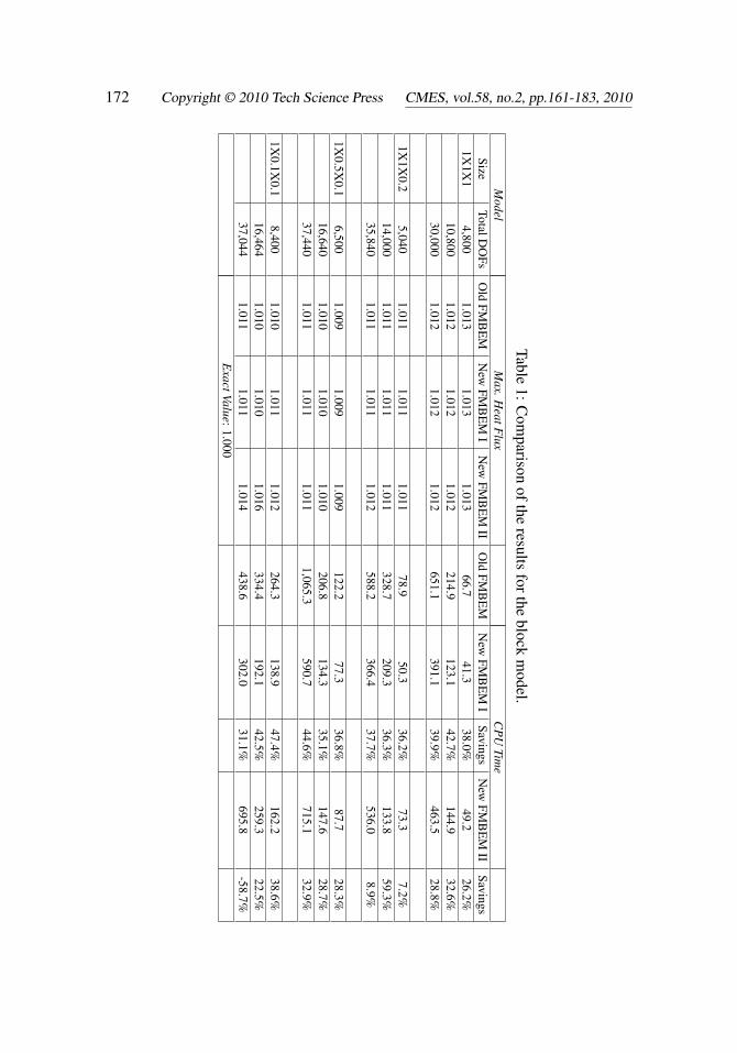
First, we use a block model (Figure 6) with different aspect ratios to study a heatconduction problem with the developed new adaptive fast multipole BEM. Thefront and back surfaces (with the normal in the +x or –x direction) are applied witha temperature with its value equal to that of the x-coordinate of the surface. On allthe other surfaces, a zero flux condition is imposed. The maximum heat flux on thefront surface is computed using the previous fast multipole BEM code (termed OldFMBEM). The Old FMBEM includes the four list adaptive algorithm. The code hasbeen first described by Shen and Liu (Liu and Shen 2007; Shen and Liu 2007); thenew adaptive fast multipole BEM code with L2 modification only (New FMBEMI), and the new adaptive fast multipole BEM code with both L2 modification andthe adaptive tree (New FMBEM II). In all the cases, only the conventional BIE isapplied, 15 terms are used in the expansions, the number of elements allowed in aleaf is set to 100, and the tolerance for convergence is set at 10−6.

Table 1 shows the results for the block model with four different sizes, changingfrom a bulky shape (a cube), to flat shapes, and finally to a slender shape. Thecomputed maximum values of the heat flux (normal derivative of the temperaturein this case) on the front surface using the three versions of the fast multipole BEMare reported in the table. From these results, it is seen that the accuracy of the newadaptive fast multipole BEM codes, with either the L2 modification only or boththe L2 modification and the adaptive tree, is equivalent to that of the previous fastmultipole BEM code. The error of about 1% in all the results can be further reducedwith tightened parameters in the solutions.

The CPU time comparison of the three versions of the fast multipole BEM is alsoreported in Table 1. The effect of the L2 modification for the fast multipole BEM(New FMBEM I) is most evident in all the models studied, with the reductions


Table1:C

omparison

oftheresults

fortheblock

model.

Model

Max.H

eatFlux

CP

UTim

eSize

TotalDO

FsO

ldFM

BE

MN

ewFM

BE

MI

New

FMB

EM

IIO

ldFM

BE

MN

ewFM

BE

MI

SavingsN

ewFM

BE

MII

Savings1X

1X1

4,8001.013

1.0131.013

66.741.3

38.0%49.2

26.2%10,800

1.0121.012

1.012214.9

123.142.7%

144.932.6%

30,0001.012

1.0121.012

651.1391.1

39.9%463.5

28.8%

1X1X

0.25,040

1.0111.011

1.01178.9

50.336.2%

73.37.2%

14,0001.011

1.0111.011

328.7209.3

36.3%133.8

59.3%35,840

1.0111.011

1.012588.2

366.437.7%

536.08.9%

1X0.5X

0.16,500

1.0091.009

1.009122.2

77.336.8%

87.728.3%

16,6401.010

1.0101.010

206.8134.3

35.1%147.6

28.7%37,440

1.0111.011

1.0111,065.3

590.744.6%

715.132.9%

1X0.1X

0.18,400

1.0101.011

1.012264.3

138.947.4%

162.238.6%

16,4641.010

1.0101.016

334.4192.1

42.5%259.3

22.5%37,044

1.0111.011

1.014438.6

302.031.1%

695.8-58.7%

ExactValue:1.000


Figure 6: A block model for a heat conduction problem.

in the CPU time ranging from 31-47% as compared with the previous version (OldFMBEM). On the other hand, the effect of the fast multipole BEM with the adaptivetree in addition to the L2 modification (New FMBEM II) is mixed for all the modelsstudied in this case. In fact, the reductions of the CPU time in general are less thanthose with the L2 modification only version of the code, except for one case whenit delivered a 59% reduction for the flat domain. In another case, however, a -59% reduction for the slender domain is registered. These mixed results for thenew adaptive fast multipole BEM code with both L2 modification and adaptivetree may stem from the overhead and variations associated with the adaptive treeand the relatively small model sizes used. The advantage of the adaptive tree willemerge in the following two examples, in which larger models will be studied. Inaddition, the drop in the effectiveness of the adaptive tree may be caused by theless effective preconditioners associated with the adaptive tree. With the adaptivetree, elements in a slender BEM model are more uniformly distributed among allthe leaves, leading to smaller numbers of elements per leaf. This is good for thememory usage because fewer coefficients will need to be computed and stored forthe preconditioner, but is less effective in preconditioning the system.

5.2 A Comb-Drive Model

Next, we study the same comb-drive model as used in Ref. (Liu and Shen 2007)to demonstrate the efficiency of the new fast multipole BEM. In this simplifiedcomb-drive model, conducting beams of identical sizes are placed parallel to eachother and with a small offset in the direction along the length of the beams. Thebeams are applied with a constant positive or negative voltage alternately and the


electrical charge density is computed on the surfaces of the beams in this exteriordomain problem. With the increase of the number of the beams in the model, theentire model becomes either a 1-D slender structure or a 2-D flat structure, both ofwhich can potentially benefit from the adaptive tree structure implemented in thenew fast multipole BEM. The dimensions and spacing of the beams are given inRef. (Liu and Shen 2007) and each beam is discretized with 3260 elements. In thisexample, the dual BIE (Liu and Shen 2007) is applied, 10 terms are used in theexpansions, the number of elements allowed in a leaf is set at 100 and the tolerancefor convergence is 10−4.

BEM models with 3, 7, 11, . . . , and up to 101 beams are solved using the previ-ous fast multipole BEM code (Old FMBEM) (Liu and Shen 2007; Shen and Liu2007); the new adaptive fast multipole BEM code with L2 modification only (NewFMBEM I), and the new adaptive fast multipole BEM code with both L2 modifi-cation and adaptive tree (New FMBEM II). The BEM models and the CPU timecomparison results are given in Table 2. Again, the New FMBEM I code con-sistently delivered reductions of the CPU time ranging from 21-29%, whereas theNew FMBEM II code delivered reductions of the CPU time ranging from 2-30%,for BEM models with DOFs below 200,000. The large variations of the effectsof the New FMBEM II are caused by the variations of the tree structure when theproblem size changes. For the last two BEM models (with DOFs above 200,000)for which the new adaptive tree code is more efficient in the usage of the memoriesand thus more coefficients in the direct evaluation can be saved for re-use (Shenand Liu 2007), the savings in the CPU time are significant as compared with theOld FMBEM and the New FMBEM I codes, both of which require larger memoryfor larger models.

A contour plot of the computed charge density for the 101-beam model is givenin Figure 7. The differences in the BEM results with the old version and the newversions of the adaptive fast multipole BEM are less than 1% which is indistin-guishable on these contour plots.

5.3 A Torsional MEMS Model

Next, we study a torsional accelerometer MEMS model (Figure 8) which is againan exterior electrostatic problem used to study the charge density distributions onthe MEMS device. The model is discretized with 696,486 boundary elements andthe mesh pattern is shown in Figure 9. For the boundary conditions, the substrate(the stationary part, shown in blue in Figure 8) is applied with a negative voltageand the rotor (the moving part, shown in red in Figure 8) is applied with a positivevoltage. The new adaptive fast multipole BEM code is used to calculate the chargedensities on this MEMS device. In this case, the dual BIE formulation is applied, 6


Tabl

e2:

Com

pari

son

ofth

eC

PUtim

esfo

rthe

com

b-dr

ive

mod

els.

Mod

els

CP

UTi

mes

Num

bero

fBea

ms

Tota

lDO

FsO

ldFM

BE

MN

ewFM

BE

MI

Savi

ngs

New

FMB

EM

IISa

ving

s3

9,78

044

.333

.125

.3%

35.0

21.0

%7

22,8

2011

9.5

86.7

27.5

%11

7.0

2.0%

1135

,860

212.

615

1.2

28.9

%16

1.2

24.2

%15

48,9

0029

4.0

216.

126

.5%

206.

729

.7%

2374

,980

474.

635

4.5

25.3

%39

8.8

16.0

%31

101,

060

668.

252

3.3

21.7

%51

3.1

23.2

%43

140,

180

969.

275

2.7

22.3

%78

6.6

18.8

%55

179,

300

1,42

4.9

1,12

8.7

20.8

%1,

060.

625

.6%

6521

1,90

05,

299.

44,

170.

221

.3%

1,32

0.8

75.1

%10

132

9,26

08,

852.

68,

070.

08.

8%3,

615.

959

.2%


Figure 7: Computed charge densities on a comb-drive model with 101 beams thatare discretized with 329,260 boundary elements.

terms are used in the expansions, the maximum number of elements in a leaf is setto 100 and the tolerance for convergence is set to 10−4.

Figure 8: A torsional accelerometer MEMS model.

Figure 10 is a plot of the computed charge density on the device, which shows theconverged result as compared with those using BEM models with smaller numbersof elements. The dual BIE (Liu and Shen 2007; Shen and Liu 2007) is used insolving this large BEM model with 696,486 DOFs on the Dell® Precision desktopPC. The CPU time is 4686 sec with the new fast multipole BEM with both theL2 modification and the adaptive tree, and is 7024 sec with the new fast multipole


Figure 9: Mesh pattern for the torsional accelerometer MEMS model discretizedwith 696,486 boundary elements.

Figure 10: Computed charge density on the torsional accelerometer MEMS model.

BEM with the L2 modification only. The advantages of using the adaptive treeemerged for this large BEM model of a flat structure. Further investigation revealsthat the number of the tree levels is 5 with the adaptive tree and is 7 with the L2modification only version for this model. Therefore the numbers of the M2M, M2Land L2L translations are fewer with the adaptive tree version than those with the


L2 modification only version.

5.4 An Acoustic Radiation Model

As the last example, we use a 3-D acoustic wave problem to show that the newadaptive fast multipole algorithm can also be applied to improve the fast mul-tipole BEM for solving other types of problems. In this case the baseline codeused for comparison is the one that uses the O(p3) transformations introduced byGumerov (Gumerov and Duraiswami 2003) in the fast multipole method for solvingHelmholtz equations, where p is the expansion order. This code has been describedin the Ref. (Bapat, Shen et al. 2009). See also Ref. (Brancati, Aliabadi et al. 2009)for a recent paper on comparison of the fast multipole BEM with the adaptive crossapproximation method for solving 3-D acoustic problems.

The problem considered is the acoustic radiation from a slender box vibrating witha uniform boundary velocity. The dimensions of the box are 1x1x10. The valueof the nondimensional wavenumber is 10 (wavenumber k = 1). The model with aBEM mesh is shown on the left in Figure 11. The model has an increasing numberof elements and is solved on the Dell® Precision Desktop PC. In this case, 16 termsare used in the expansions, the maximum number of elements in a leaf is set to 50and the tolerance for convergence is set to 10−5.

The computed sound pressure on the boundary is shown on the right in Figure 11.The CPU time is shown in Figure 12. As predicted, the CPU time is observed to bethe least when we use L2 modification in conjunction with the use of the adaptivetree. The L2 modification alone is seen to improve the efficiency of the code by25-50% depending on the particular discretization. In addition, the adaptive treestructure is seen to have a reduction in the CPU time by about 15-20% dependingon the model size.

6 Discussions

A new adaptive fast multipole algorithm based on a modified L2 list (or the inter-action list), the four list adaptive algorithm and an adaptive tree structure is pre-sented in this paper. This algorithm uses many of the existing efficient algorithms.Appropriate changes necessary to combine all the existing techniques have beendiscussed. This combination is faster than all the individual algorithms or modifi-cations. The L2 modification, introduced in this paper, can consistently save a sig-nificant amount of CPU time in computing the M2L translations and the adaptivetree can potentially reduce the total CPU time for large models of slender and flatthin structures. This new adaptive fast multipole algorithm has been implementedin the fast multipole BEM code based on the new version of the FMM (using M2X,


Figure 11: Acoustic radiation from a slender structure (the mesh and computedsound pressure).

0

50

100

150

200

250

300

0 10,000 20,000 30,000 40,000 50,000 60,000

CP

U T

ime

(sec

.)

DOFs

Baseline code

Baseline + L2

Baseline + L2 + Adaptive tree

Figure 12: CPU time for the acoustic radiation model.


X2X, and X2L translations) for 3-D potential problems and an O(p3) code for 3-Dacoustic wave problems.

Several numerical examples are presented to demonstrate the usefulness and ef-ficiency of the proposed new adaptive fast multipole algorithm. About 30-40%improvements in the computational efficiency are achieved with the L2 modifica-tion. The adaptive tree, a promising data structure for the FMM, has also beeninvestigated in this paper. Results with the adaptive tree structure are mixed. Whilethe adaptive tree does not provide noticeable positive effects on the efficiency forsmaller BEM models, it does show some advantages for larger BEM models, espe-cially for MEMS models which are thin structures, and for acoustic problems. Theimplementation of L2 modification in existing codes is straightforward and it canbe used to accelerate many other existing fast multipole BEM codes.

Acknowledgement: The support from US National Science Foundation throughthe grant CMS-0508232 is acknowledged. The authors also thank Mr. Bo Bi forhis help in building the torsional accelerometer MEMS CAD model used in thiswork.

References

Anderson, R. J. (1999): Tree data structures for N-body simulation. SIAM J.Comput. 28: 1923–1940.

Aoki, S., K. Amaya, M. Urago, A. Nakayama (2004): Fast multipole boundaryelement analysis of corrosion problems. CMES: Computer Modeling in Engineer-ing and Sciences 6(2): 123-132.

Bapat, M. S., L. Shen, Y. J. Liu (2009): Adaptive fast multipole boundary ele-ment method for three-dimensional half-space acoustic wave problems. Engineer-ing Analysis with Boundary Elements 33(8-9): 1113-1123.

Brancati, A., M. H. Aliabadi, I. Benedetti (2009): Hierarchical adaptive cross ap-proximation GMRES technique for solution of acoustic problems using the bound-ary element method. CMES: Computer Modeling in Engineering & Sciences 43(2):149-172.

Chen, X. L., Y. J. Liu (2001): Thermal stress analysis of multi-layer thin films andcoatings by an advanced boundary element method. CMES: Computer Modelingin Engineering & Sciences 2(3): 337-350.

Cheng, H., L. Greengard, V. Rokhlin (1999): A fast adaptive multipole algorithmin three dimensions. Journal of Computational Physics 155: 468-498.

Fu, Y., K. J. Klimkowski, G. J. Rodin, E. Berger, J. C. Browne, J. K., Singer,


R. A. V. D. Geijn, K. S. Vemaganti (1998): A fast solution method for three-dimensional many-particle problems of linear elasticity. International Journal forNumerical Methods in Engineering 42: 1215-1229.

Gomez, J. E., H. Power (1997): A multipole direct and indirect BEM for 2D cavityflow at low Reynolds number. Engineering Analysis with Boundary Elements 19:17-31.

Greengard, L. F. (1988): The Rapid Evaluation of Potential Fields in ParticleSystems. Cambridge, The MIT Press.

Greengard, L. F., V. Rokhlin (1987): A fast algorithm for particle simulations.Journal of Computational Physics 73(2): 325-348.

Gumerov, N. A., R. Duraiswami (2003): Recursions for the computation of mul-tipole translation and rotation coefficients for the 3-D Helmholtz equation. SIAMJ. Sci. Comput. 25(4): 1344-1381.

Liu, Y. J. (2005): A new fast multipole boundary element method for solving large-scale two-dimensional elastostatic problems. International Journal for NumericalMethods in Engineering 65(6): 863-881.

Liu, Y. J. (2008): A fast multipole boundary element method for 2-D multi-domainelastostatic problems based on a dual BIE formulation. Computational Mechanics42(5): 761-773.

Liu, Y. J. (2009): Fast Multipole Boundary Element Method - Theory and Appli-cations in Engineering. Cambridge, Cambridge University Press.

Liu, Y. J., H. Fan (2002): Analysis of thin piezoelectric solids by the bound-ary element method. Computer Methods in Applied Mechanics and Engineering191(21-22): 2297-2315.

Liu, Y. J., N. Nishimura (2006): The fast multipole boundary element methodfor potential problems: a tutorial. Engineering Analysis with Boundary Elements30(5): 371-381.

Liu, Y. J., N. Nishimura, Y. Otani (2005): Large-scale modeling of carbon-nanotube composites by the boundary element method based on a rigid-inclusionmodel. Computational Materials Science 34(2): 173-187

Liu, Y. J., N. Nishimura, Y. Otani, T. Takahashi, X. L. Chen, H. Munakata(2005): A fast boundary element method for the analysis of fiber-reinforced com-posites based on a rigid-inclusion model. Journal of Applied Mechanics 72(1):115-128.

Liu, Y. J., N. Nishimura, D. Qian, N. Adachi, Y. Otani, V. Mokashi (2008):A boundary element method for the analysis of CNT/polymer composites with acohesive interface model based on molecular dynamics. Engineering Analysis with


Boundary Elements 32(4): 299–308.

Liu, Y. J., L. Shen (2007): A dual BIE approach for large-scale modeling of 3-Delectrostatic problems with the fast multipole boundary element method. Interna-tional Journal for Numerical Methods in Engineering 71(7): 837–855.

Luo, J. F., Y. J. Liu, E. J. Berger (1998): Analysis of two-dimensional thin struc-tures (from micro- to nano-scales) using the boundary element method. Computa-tional Mechanics 22: 404-412.

Mammoli, A. A., M. S. Ingber (1999): Stokes flow around cylinders in a boundedtwo-dimensional domain using multipole-accelerated boundary element methods.International Journal for Numerical Methods in Engineering 44: 897-917.

Nishimura, N. (2002): Fast multipole accelerated boundary integral equation meth-ods. Applied Mechanics Reviews 55(4 (July)): 299-324.

Nishimura, N., K. Yoshida, S. Kobayashi (1999): A fast multipole boundary inte-gral equation method for crack problems in 3D. Engineering Analysis with Bound-ary Elements 23: 97-105.

Peirce, A. P., J. A. L. Napier (1995): A spectral multipole method for efficient so-lution of large-scale boundary element models in elastostatics. International Jour-nal for Numerical Methods in Engineering 38: 4009-4034.

Rokhlin, V. (1985): Rapid solution of integral equations of classical potential the-ory. J. Comp. Phys. 60: 187-207.

Shen, L., Y. J. Liu (2007): An adaptive fast multipole boundary element methodfor three-dimensional acoustic wave problems based on the Burton-Miller formu-lation. Computational Mechanics 40(3): 461-472.

Shen, L., Y. J. Liu (2007): An adaptive fast multipole boundary element methodfor three-dimensional potential problems. Computational Mechanics 39(6): 681-691.

Urago, M., T. Koyama, K. Takahashi, S. Saito and Y. Mochimaru (2003):Fast multipole boundary element method using the binary tree structure with tightbounds: application to a calculation of an electrostatic force for the manipulationof a metal micro particle. Engineering Analysis with Boundary Elements 27(8):835-844.

Wang, H. T., G. Hall, S. Y. Yu, Z. H. Yao (2008): Numerical simulation ofgraphite properties using X-ray tomography and fast multipole boundary elementmethod. CMES: Computer Modeling in Engineering and Sciences 37(2): 153-174.

Wang, H. T., Z. H. Yao (2005): A new fast multipole boundary element method forlarge scale analysis of mechanical properties in 3D particle-reinforced compositesCMES: Computer Modeling in Engineering and Sciences 7(1): 85-96.


Yarvin, N., V. Rokhlin (1998): Generalized Gaussian quadratures and singularvalue decompositions of integral operators. SIAM J. Sci. Computing 20: 699-718.

Yoshida, K. (2001): Applications of Fast Multipole Method to Boundary IntegralEquation Method. Department of Global Environment Engineering. Kyoto, Japan,Kyoto University: 137.

Zhang, J., M. Tanaka (2007): Adaptive spatial decomposition in fast multipolemethod. Journal of Computational Physics 226(1): 17-28.

a new adaptive algorithm for the fast multipole boundary

Documents