does land fragmentation affect farm performance? a …ageconsearch.umn.edu/bitstream/207854/2/wp...

Does land fragmentation affect farm performance?

A case study from Brittany, France

Laure LATRUFFE, Laurent PIET

Working Paper SMART – LERECO N°13-04

April 2013

UMR INRA-Agrocampus Ouest SMART (Structures et Marchés Agricoles, Ressources et Territoires)

UR INRA LERECO (Laboratoires d’Etudes et de Recherches en Economie)

Working Paper SMART – LERECO N°13.04

Les Working Papers SMART-LERECO ont pour vocation de diffuser les recherches

conduites au sein des unités SMART et LERECO dans une forme préliminaire

permettant la discussion et avant publication définitive. Selon les cas, il s'agit de

travaux qui ont été acceptés ou ont déjà fait l'objet d'une présentation lors d'une

conférence scientifique nationale ou internationale, qui ont été soumis pour publication

dans une revue académique à comité de lecture, ou encore qui constituent un chapitre

d'ouvrage académique. Bien que non revus par les pairs, chaque working paper a fait

l'objet d'une relecture interne par un des scientifiques de SMART ou du LERECO et par

l'un des deux éditeurs de la série. Les Working Papers SMART-LERECO n'engagent

cependant que leurs auteurs.

The SMART-LERECO Working Papers are meant to promote discussion by

disseminating the research of the SMART and LERECO members in a preliminary form

and before their final publication. They may be papers which have been accepted or

already presented in a national or international scientific conference, articles which

have been submitted to a peer-reviewed academic journal, or chapters of an academic

book. While not peer-reviewed, each of them has been read over by one of the scientists

of SMART or LERECO and by one of the two editors of the series. However, the views

expressed in the SMART-LERECO Working Papers are solely those of their authors.


Does land fragmentation affect farm performance?

A case study from Brittany, France

Laure LATRUFFE

INRA, UMR1302 SMART, F-35000 Rennes, France

Laurent PIET

INRA, UMR1302 SMART, F-35000 Rennes, France

Acknowledgments Financial support from FP7 project Factor Markets (Comparative Analysis of Factor Markets for Agriculture across the Member States) grant agreement n°245123-FP7-KBBE-2009-3 is acknowledged. The authors thank the Service de la Statistique et de la Prospective from the French ministry of Agriculture for providing the FADN 2007 database. The authors also thank Hugo Juhel and Yann Desjeux for their help and Pierre Dupraz for his useful suggestions.

Auteur pour la correspondance / Corresponding author

Laurent Piet INRA, UMR SMART 4 allée Adolphe Bobierre, CS 61103 35011 Rennes cedex, France Email: [email protected] Téléphone / Phone: +33 (0)2 23 48 53 83 Fax: +33 (0)2 23 48 53 80

Les Working Papers SMART-LERECO n’engagent que leurs auteurs. The views expressed in the SMART-LERECO Working Papers are solely those of their authors

1


Does land fragmentation affect farm performance? A case study from Brittany, France

Abstract

Agricultural land fragmentation is widespread around the world and may affect farmers’ decisions and therefore have an impact on the performance of farms, in either a negative or a positive way. We investigated this impact for the western region of Brittany, France, in 2007. To do so, we regressed a set of performance indicators on a set of fragmentation descriptors. The performance indicators (production costs, yields, revenue, profitability, technical and scale efficiency) were calculated at the farm level using Farm Accountancy Data Network (FADN) data, while the fragmentation descriptors were calculated at the municipality level using data from the cartographic field pattern registry (RPG). The various fragmentation descriptors enabled not only the traditional number and average size of plots, but also their scattering in the geographical space, to be taken into account. Our analysis highlights the fact that the measures of land fragmentation usually used in the literature do not reveal the whole set of significant relationships with farm performance and that, in particular, measures accounting for distance should be taken into consideration more systematically.

Keywords: agricultural land fragmentation, farm performance, cartographic field pattern registry, France

JEL classifications: Q12, Q15, D24

Le morcellement parcellaire affecte-t-il la performance des exploitations agricoles ? Application au cas de la Bretagne, France

Résumé

Le morcellement du parcellaire agricole est un phénomène répandu qui peut influencer les décisions des agriculteurs et donc avoir un impact, positif ou négatif, sur la performance des exploitations. Nous avons étudié cet impact pour la région Bretagne en 2007. Pour ce faire, nous avons régressé un ensemble d’indicateurs de la performance sur un ensemble de descripteurs du morcellement. Les indicateurs de performance (coûts de production, rendements, revenu, rentabilité, efficacité technique et d’échelle) ont été calculés à l’échelle de l’exploitation à partir des données du Réseau d’Information Comptable Agricole (RICA), tandis que les descripteurs de morcellement ont été calculés à l’échelle communale à partir des données du Registre Parcellaire Graphique (RPG). Les différents descripteurs de morcellement utilisés ont permis de prendre en compte non seulement le nombre et la taille moyenne des îlots, traditionnellement étudiés, mais également leur dispersion géographique. Notre analyse met en évidence que les mesures du morcellement généralement utilisées dans la littérature ne permettent pas de mettre en évidence toutes les relations significatives avec la performance et que, en particulier, tenir compte des effets de la distance devrait être plus systématique.

Mots-clés : morcellement parcellaire agricole, performance des exploitations agricoles, registre parcellaire graphique, France

Classifications JEL : Q12, Q15, D24

2


Does land fragmentation affect farm performance? A case study from Brittany, France

1 Introduction

Fragmentation of agricultural land is widespread around the world and results from various

institutional, political, historical and sociological factors, such as inheritance laws,

collectivisation and consolidation processes, transaction costs in land markets, urban

development policies, and personal valuation of land ownership (King and Burton, 1982;

Blarel et al., 1992). Farm land fragmentation (LF) is a complex concept that encompasses five

dimensions covering: i) number of plots farmed; ii) plot size; iii) the shape of plots; iv)

distance of the plots from the farm buildings; v) distances between plots (or plot scattering).

From the public economics perspective, LF may generate both positive and negative

externalities: it may increase biodiversity and society’s economic value of landscape but, in

contrast, it may induce additional trips by farmers which may result in extra roadwork, road

safety issues, greenhouse gas emissions, etc. However, first and foremost, LF may affect

farmers’ production decisions and therefore have an impact on the performance of farms. This

impact may be negative or positive. There are several reasons why the impact may be

negative. Firstly, LF may exacerbate conflicts regarding labour allocation on the farm: it takes

time to travel from one plot to another while the labour force could be undertaking more

productive tasks. Secondly, production costs may be increased as LF may require additional

equipment, secondary farm buildings and/or external service expenses. Thirdly, LF may

restrict the choice of production and constrain management practices, especially in terms of

herd management. This could be particularly true for regions where dairy production prevails,

such as Brittany, a region in the west of France. Fourthly, investments for soil quality

improvement, such as drainage, may be reduced on remote plots, potentially reducing yields.

However, the impact of LF on farm performance may be positive. This is the case if LF leads

to an increased diversity in land quality so that the allocation of crops across plots may be

optimised, resulting in potentially higher overall yields. In addition, LF may give greater

opportunities for risk diversification, thereby reducing production risks at the farm level. For

example, a fragmented farm would be less affected by a pest outbreak that spreads on

contiguous plots only.

Several authors have tested empirically the effects of LF on the performance of farms. For

example, Jabarin and Epplin (1994) investigated the impact of LF on the production cost of

3


4

wheat in Jordan. In China, Nguyen et al. (1996), Wan and Cheng (2001) and Tan et al. (2010)

investigated the effect of LF on the productivity of major crops, crop output of rural

households, and technical efficiency of rice producers in the South-East of the country,

respectively. Kawasaki (2010) evaluated both the costs and benefits of LF in the case of rice

production in Japan, similarly to Rahman and Rahman (2008) in Bangladesh. Parikh and Shah

(1994) investigated the influence of LF on the technical efficiency of farms in the North-West

Frontier Province of Pakistan, while Manjunatha et al. (2013) carried out a similar

investigation in India. In Europe, Di Falco et al. (2010) analysed how LF affects farm

profitability in Bulgaria and Del Corral et al. (2011) analysed how LF affects the profits of

Spanish dairy farms.

In most of this research, LF is represented by the number of plots and/or their average size.

These two variables are employed either directly or indirectly by the use of more elaborate

measures, such as the Simpson index or the Januszewski index (which are defined further in

the text). However, these variables do not account for all dimensions of LF and may not

capture all the constraints that LF imposes on production systems. There are a few exceptions

to the use of these sole variables. For example, Tan et al., 2010 considered in addition the

average distance from the plots to the homestead, while Gonzalez et al. (2007) used more

elaborate measures of LF (which accounted for the size, shape and dispersion of plots) to

study the productivity gains from land consolidation. However, in this latter case, these

measures were not tested on a real sample of farms, but instead were applied to a hypothetical

dataset of farms.

The objective of the paper is to analyse the influence of LF on the performance of farms in the

case of one French region, the Western region of Brittany, or ‘Bretagne’. This is a NUTS2

region which is composed of four NUTS3 regions (the ‘départements’), namely ‘Côtes-

d’Armor’, ‘Finistère’, ‘Ille-et-Vilaine’ and ‘Morbihan’.1 As in many other regions and

countries, agricultural land is very fragmented in Brittany. For example in 2007, according to

the cartographic field pattern registry (‘Registre Parcellaire Graphique’ or RPG) introduced in

France in 2002 following the European Council Regulation No 1593/2000 (European

Commission, 2000), Brittany farms were composed on average of 14 plots, with a mean plot

size of 4.35 ha. Twenty-five percent of the farms had 18 plots or more, and 25% of these plots

1 The Nomenclature of Territorial Units for Statistics (NUTS) provides a single uniform breakdown of territorial units for the production of regional statistics for the European Union (EU). (Source: http://epp.eurostat.ec.europa.eu/portal/page/portal/nuts_nomenclature/introduction)


had an average area of 2.42 ha or less. Such figures are quite similar to the national averages

for France. In this paper, the relationship between LF and farm performance is investigated

for the year 2007 using several performance indicators (production costs, yields, financial

results and technical efficiency) calculated from farm-level data, and various LF indicators

calculated at the municipality level using data from the RPG. The various fragmentation

indicators enable the traditional measures of plot number and mean size of plots, as well as

the scattering of plots, to be accounted for.

The paper is structured as follows. Section 2 describes the data and explains the methodology

used to calculate the various indicators of performance and of LF. Section 3 presents the

methodology used to investigate the effect of LF on performance and the results of the

empirical analysis. Section 4 concludes.

2. Data and methodology

2.1. Measuring farm performance

As mentioned above, we used farm-level data for the calculation of farm performance

indicators, and municipality-level averages for the calculation of LF. More precisely, we

investigated the relationship between farm performance for a sample of farms, and LF of the

municipality where the sample farms are located. The underlining assumption is that a farm’s

LF is positively correlated with the LF in the municipality where the farmstead is located. The

studied farms were extracted from the French Farm Accountancy Data Network (FADN)

2007 database. The FADN database, managed by the French Ministry of Agriculture, contains

structural and bookkeeping information for a five-year rotating panel of professional farms. In

2007, 480 farms of the FADN sample were located in Brittany. Among those 480 farms we

excluded ten farms which used no land and one farm with inconsistent capital data. The final

sample thus consisted of 469 farms. Figure 1 shows the location of the municipalities of the

469 FADN Brittany farms.

5


Figure 1: Brittany NUTS3 regions and studied municipalities

Source: authors’ calculations – ©IGN 2011, Geofla®

Table 1: Main characteristics of the farms in the FADN sample used (469 farms)

Share of farms in the sample (%) According to their main production

Field crops Dairy Other grazing livestock Granivores Mixed (crops and livestock) Other crops

13 29 14 27 11 6

In areas with nitrate pollution zoning restrictions 4 Mean Std. deviation Minimum Maximum

Utilised agricultural area (ha) 62.36 44.93 0.12 398.96 Number of full time labour equivalents 2.44 2.57 1.00 23.96 Number of livestock units 244.85 359.62 0.00 2,522.11 Share of land rented in (%) 77 33 0 100 Share of hired labour (%) 15 25 0 100

Source: authors’ calculations based on the French FADN 2007 database

Table 1 describes the sample of the 469 farms used to analyse the relationship between farm

performance and LF. It shows the distribution of these farms according to their main type of

production, according to the European definition of type of farming (European Commission,

2010), where the main production is the one which provides at least two-thirds of the farm’s

gross standard margin. The distribution reflects Brittany’s agriculture where dairy, poultry

6


and pig breeding prevail: 29% of the sample specialised in dairy production, and 27% in

granivores production. Mixed crop and livestock farming (generally the production of cows’

milk and field crops) accounted for 11% of the sample, and the breeding of other grazing

livestock (goats and sheep) for 14%. Finally, for 13% of the sample farms the main

production was field crops, and for another 6% the main production was crops other than field

crops (mainly vegetables).

Figure 2: Main productions in Brittany’s municipalities

Source: authors’ calculations based on Agricultural Census 2010 – ©IGN 2011, Geofla®

Figure 2 shows the distribution of Brittany municipalities according to the main production of

each municipality based on the 2010 Agricultural Census. Granivores farms were located

principally in central and eastern Brittany, while crops were mainly produced on the coast,

and grazing livestock breeding took place mainly in the western part of the region. Four

percent of the farms in the FADN sub-sample used were located in areas subject to nitrate

pollution zoning regulations (Table 1). In 2007, the studied farms utilised on average 62.4 ha,

a figure greater than the average for the whole farm population in Brittany (47.3 ha) but close

to the average of Brittany’s commercial farm sub-population (60.0 ha) (2010 Agricultural

7


Census). The farms in our sample used, on average, 2.4 full time equivalents calculated as

Annual Working Units (AWU; where 1 AWU corresponds to 1,200 hours of labour per year).

This is higher than the region’s average (1.7 AWU) and similar to the region’s commercial

farms’ average (2.1 AWU) (2010 Agricultural Census). The average number of livestock

units (calculated using the European standard coefficients applied to each livestock type) on

the sample farms was 244.9. This relatively high figure is due to the numerous farms in

Brittany specialised in livestock and, in particular, to the poultry and pig head numbers. On

average, farms rented in 77% of their utilised area and employed 15% of hired labour force.

Several indicators of farm performance were computed for each farm in the sample. Firstly,

various categories of production costs were calculated per farm and per unit of utilised area.

These consisted of costs of fertilisers, seeds, pesticides, fuel, intermediate consumption and

hired labour. Secondly, two production yields were calculated: wheat yield in tons of wheat

produced per hectare of wheat cultivated; and milk yield in litres of milk produced per cow.

Thirdly, four revenue or profitability results were calculated per farm and per unit of utilised

area: the farm gross product, composed of farm sales and insurance compensations; the farm

gross margin, obtained from the farm gross product minus variable costs specific to crop and

livestock production; the farm operating surplus, obtained from the farm gross margin minus

land, labour and insurance costs; and the farm pre-tax profit, given by the farm operating

surplus minus depreciation and interest, and before taxes are deducted. Subsidies were not

included in the farm gross product, and therefore not included either in the three profitability

indicators. Finally, technical efficiency and scale efficiency were calculated for each farm.

Technical efficiency assesses how far farms are located from the maximum production

frontier for a given combination of inputs. It is a more complex measure than partial

productivity indicators such as yields, since it relates all outputs produced to all inputs used

on the farm. Technical efficiency is composed of pure technical efficiency (that is to say,

whether farmers operate their farm efficiently) and of scale efficiency (that is to say, whether

the farm’s production scale is optimal). Technical and scale efficiencies were computed using

the non-parametric method Data Envelopment Analysis (DEA) which employs linear

programming to construct a frontier that envelops the data used (Charnes et al., 1978).

Efficiency scores obtained by DEA are between one – for a fully efficient farm (i.e., a farm

located on the efficient frontier) – and zero, with smaller scores indicating lower efficiency.

Since the efficient frontier depends on the sample used, the efficiency scores may be

overestimated if the most highly performing farms in the population are not included. For this

8


reason, we constructed the efficient frontier for the whole Brittany sample (469 farms). We

merged all types of farming into one sample to overcome the limited sizes of the type of

farming sub-samples. The DEA model was output-oriented (so that farms were assumed to

maximise their output level, given input levels). The model had one single output, namely the

farm output produced in Euros, and four inputs: the utilised area in hectares; the labour used

in AWU; the intermediate consumption in Euros; and the capital value in Euros. Under the

assumption that farms operated under constant returns to scale, the total technical efficiency

score for each farm was obtained. Total technical efficiency was then decomposed into pure

technical efficiency and scale efficiency. The calculation of the pure technical efficiency was

made under the assumption that farms operated under variable returns to scale, and indicated

the efficiency of farmers’ practices irrespective of farm size. By contrast, scale efficiency,

which was calculated for each farm as the ratio between its total technical efficiency and its

pure technical efficiency, revealed whether the farm operated at the optimal scale of

production.

Table 2: Performance of the farms in the FADN sub-sample used

Farm performance indicator Average value Number of observations per farm per hectare

Production costs (Euros) Fertiliser cost Seed cost Pesticide cost Fuel cost Intermediate consumption cost Hired labour cost

7,083.73 7,724.19 6,010.70 4,768.39

194,364.50 13,622.62

341.87

1,143.79 225.95 156.43

13,542.45 3,360.09

469 469 469 469 469 469

Yields Wheat yield (tons / hectare) Milk yield (litres / cow)

5.3

7,043

342 269

Revenue and profitability without farm subsidies (Euros) Gross product Gross margin Operating surplus Pre-tax profit

297,385.60 103,021.10 63,214.24 13,697.48

23,901.72 10,359.27

5,258.55 1,756.50

469 469 469 469

Efficiency scores Total technical efficiency Pure technical efficiency Scale efficiency

0.595 0.680 0.883

469 469 469

Source: authors’ calculations based on the French FADN 2007 database

Table 2 presents the descriptive statistics of the performance indicators for the 469 sample

farms. Among these, 342 farms (73% of the sample) produced wheat with an average yield of

9


10

5.3 tons per hectare, and 269 farms (57% of the sample) produced milk with an average yield

of 7,043 litres per cow. The 469 farms generated on average almost 1,800 Euros per hectare

of pre-tax profit without subsidies. Their total technical efficiency score was 0.595 on

average, indicating that they could increase their output by 40.5% without increasing their

input use.

2.2. Measuring land fragmentation

LF was measured using the RPG put in place in France in 2002 following the European

Council Regulation No 1593/2000 (European Commission, 2000). This is a Geographic

Information System (GIS) database which is maintained by the ‘Agence de Service et de

Paiement’ (ASP), a public body which gathers the field patterns declared by farmers who

apply for support under the framework of the Common Agricultural Policy (CAP)2 and which

delivers subsidies to farmers based on these declarations. In fact, farmers are not requested to

delineate each of their individual fields but rather each of their ‘plots’, which we define for

this paper as follows: a plot is a set of contiguous fields (which may or may not all bear the

same crop) which is both delimited by easily identifiable landmarks (such as agricultural

byways, roads, rivers, another plot, etc.) and is stable from year to year.

We used the 2007 registry (‘RPG anonyme ASP 2007’) which identifies 450,787 plots used

by 31,921 farms for the four NUTS3 regions of Brittany. Each farm could be categorised as

one of the following: i) a farm that was registered in one of the four Brittany NUTS3 regions

and whose plots were all located inside this one region; ii) a farm that was registered in one of

the four Brittany NUTS3 regions, but whose plots were partly located outside that region; and

iii) a farm that was registered outside Brittany but whose plots were located totally or partly

inside one of the four Brittany NUTS3 regions. We retained all farms and plots corresponding

to case i). As regards case ii), we only retained those farms whose plots were located in one of

the four NUTS3 regions directly neighbouring Brittany (namely ‘Loire-Atlantique’, ‘Maine-

et-Loire’, ‘Manche’ and ‘Mayenne’, see Figure 1) and we considered both their plots located

in Brittany and their plots located in these four directly neighbouring regions. Similarly, as

regards case iii), we retained those farms registered in one of the four above-mentioned

2 For more information on the RPG, see the dedicated pages on the website of the ASP. (http://www.asp-public.fr/?q=node/856).


NUTS3 regions directly neighbouring Brittany and we considered both their plots located in

Brittany and their plots located in one of these four directly neighbouring regions. Finally, in

order to ensure that we included ‘entire’ farms only, we excluded those farms whose total area

declared by the farmer in the RPG was 0.02 ha or more different from the area obtained from

summing the areas of each individual plot of the farm. In the end, the database used consisted

of 29,433 farms and 418,480 plots.

For each farm among these 29,433 farms, ten fragmentation descriptors were computed,

which relate to one of the five dimensions of LF as described in the introduction (the formal

definitions of the descriptors are given in the Appendix).

1. LF descriptors relating to the number of plots. One descriptor was used, namely the

number of plots on the farm ( ).

2. LF descriptors relating to the shape of plots. Two descriptors were used: the weighted

average of the shape index of the plots ( ) (Akkaya Aslan et al., 2007); and the

average of the areal form factor ( ) (Gonzalez et al., 2004).

3. LF descriptors relating to the size of plots. Three descriptors were used: the average

plot size ( ); and two more elaborate indexes, namely the Simpson index

( ) (Blarel et al., 1992; Hung et al., 2007; Kawasaki, 2010) and the Januszewski

index ( ) (King and Burton, 1982).

4. LF descriptors relating to the distance of plots from the farm. Three descriptors were

used: the average distance of a hectare from the farm ( ); and two more

elaborate indexes, namely the grouping index ( ) (Marie, 2009) and the

structural index ( ) (Marie, 2009).

5. LF descriptors relating to the scattering of plots (i.e., to the distance between plots).

One descriptor was used, namely the normalised average nearest neighbour distance

( ).

Since there was no information in the registry concerning the location of the farmsteads, we

first computed the centroid of each plot (that is, its geometric centre) and inferred from this

the barycentre of each farm (that is, its ‘centre of mass’, with the ‘mass’ associated with each

plot of the farm being the plot’s area); we then replaced the distance from the farmstead by

11


the distance from the barycentre of the farm in those LF indicators which use distance in their

definition (namely , , and ).

It should be stressed that the relationship between a descriptor and LF may be positive (i.e., a

higher value of the descriptor indicates higher fragmentation) or negative (i.e., a higher value

of the descriptor indicates lower fragmentation). As can be seen in Table 3, descriptors

positively related to LF are the number of plots, the weighted average shape index, the

Simpson index, descriptors relating to the distance from the barycentre of the farm and the

normalised average nearest neighbour distance, while descriptors negatively related to LF are

the average areal form factor, the Januszewski index and average plots size.

Table 3: Relationship between the studied descriptors and LF

Descr y r to LF iptors positivel elated Descriptors negatively related to LF Number of plots ) (

e plot sSimpson index ( ) Weighted averag hape in ) dex (

Average distance ctare ( ) eGrouping index ( )

of a h

Structural index ( ) Normalised average nearest neighbour distance ( )

Average plot areal f ctor ( ) orm fa)

Januszewski index ( ) Average plots size (

Table 4 reports descriptive statistics for the 29,433 farms in our database. On average, the

farms registered outside Brittany were the largest (their average area was 75.51 ha) and the

farms registered within Brittany were relatively similar across Brittany’s NUTS3 regions in

terms of average area (around 50 ha with a standard deviation of about 40 ha). Among the

four Brittany NUTS3 regions, ‘Côtes-d’Armor’ appears to be the most fragmented one for

most LF descriptors, followed by ‘Finistère’, ‘Ille-et-Vilaine’ and finally ‘Morbihan’. The

fragmentation of farms registered outside Brittany showed greater variation: they were

relatively fragmented when considering most descriptors but, in contrast, they presented a

lower fragmentation level in terms of mean size of plots, which was higher than that of farms

registered inside Brittany. There are two explanations for this contrasting picture. Firstly, the

sample of farms registered outside Brittany was smaller. Secondly, when considered together

they constituted a heterogeneous category (the structure and main production of farms in the

12


northern neighbour ‘Manche’ were quite different from those of the southern neighbour

‘Loire-Atlantique’).

Table 4: Descriptive statistics of the fragmentation descriptors at the farm level a

Land fragmentation descriptor

NUTS3 ‘Côtes-

d’Armor’

NUTS3 ‘Finistère’

NUTS3 ‘Ille-et-Vilaine’

NUTS3 ‘Morbihan’

Neighbouring NUTS3 regions b

All

Number of farms 7,942 6,149 8,653 6,298 391 29,433 Average farm area (ha) 49.13 54.85 47.49 52.92 75.51 51.00 (34.98) (41.64) (38.72) (39.60) (40.96) (38.82) Number of plots ( ) 15.11 14.55 12.24 12.32 14.93 13.55 (11.10) (11.10) (10.09) (9.62) (9.24) (10.56) Weigh age plot shape ted aver 1.34 1.32 1.31 1.33 1.37 1.33 index ( )

e plot arfactor ( )

(0.19) (0.17) (0.18) (0.19) (0.18) (0.19) Averag eal form

Average plots’ s )

0.044 0.044 0.044 0.044 0.042 0.044 (0.006) (0.006) (0.006) (0.006) (0.005) (0.006)

ize ( 3.67 4.41 4.53 4.90 5.74 4.37 (2.45) (3.53) (14.58) (3.65) (3.32) (8.36) Simpson index ( )

Januszewski index (

0.77 0.77 0.72 0.73 0.80 0.75 (0.22) (0.21) (0.25) (0.24) (0.15) (0.23)

) 0.37 0.37 0.42 0.41 0.34 0.39 (0.19) (0.18) (0.21) (0.20) (0.13) (0.20) Average distance of an 1,221 1,373 1,246 1,084 3,115 1,256 hectare ( ) Grouping index ( )

(1,823) (1,917) (1,844) (1,392) (3,452) (1,814)

Structural index ( )

8.93 8.92 8.74 6.84 18.01 8.55 (12.68) (11.86) (13.35) (10.33) (17.45) (12.41)

3.93 3.42 3.15 2.19 4.13 3.23 (11.52) (7.67) (7.83) (5.21) (5.56) (8.53) Normalised average nearest 1.47 1.32 1.66 1.40 2.18 1.49 neighbour distance ( (3.90) (3.76) (4.89) (3.53) (5.23) (4.14) a Except for the number of farms, averages are presented and standard deviations are shown in brackets and italic font. b Farms registered in NUTS3 regions directly neighbouring Brittany (‘Loire-Atlantique’, ‘Maine-et-Loire’, ‘Manche’ and ‘Mayenne’, see Figure 1) and whose plots are at least partly located in one of Brittany’s NUTS3 regions (‘Côtes-d’Armor’, ‘Finistère’,‘Ille-et-Vilaine’ and ‘Morbihan’).

Source: authors’ calculations based on the field pattern registry

‘RPG anonyme ASP 2007’ database

As explained in Section 2.1, we analysed the influence of average LF in the municipality

where a farm was located on the farm’s performance. To do this, we calculated the aggregated

fragmentation descriptors at the level of each municipality of the 29,433 farms in the field

pattern database. We computed the weighted average of each descriptor considering all farms

with at least one plot in , each of these farms being weighted by its share in the total operated

area of , or, formally:

13


∑ (1)

where represents one of the ten fragmentation descriptors, represents farm ’s operated

area located within municipality and ∑ is the total operated area in municipality

. Note that, because the RPG only includes farms which apply for CAP payments and

because we excluded almost 8% of the farms (2,488 out of 31,921) from the initial database

during the sample selection process (see above), the descriptors calculated at the municipality

level should be viewed only as proxies for the true farmland fragmentation of municipalities.

Table 5: Descriptive statistics of the fragmentation descriptors at the municipality level

Land fragmentation descriptor Mean Std. deviation Min Max

Studied municipalities (349 observations)Number of farms 60.56 29.73 3 200 Farmed area (ha) 3,588.31 1,844.17 53.32 11,811.04 Number of plots ( ) 19.29 7.04 8.84 62.09 Weighted average pl e in ) ot shap dex ( 1.344 0.065 1.172 1.542 Average plot are tor ( ) al form

ize fac

Average plots’ s ) 0.043 0.002 0.038 0.049

( 4.77 2.10 0.31 30.24 Simpson index ( ) Januszewski inde

0.841 0.043 0.727 0.954 x (

e) 0.302 0.047 0.158 0.422

Average distance ctare ( ) of a h 1,675 443 897 4,339 Grouping index ( ) Structural )

9.555 2.843 4.332 26.063 index (

Normalised average nearest neighbour distance (

3.179 3.751 0.780 47.152 0.986 0.281 0.415 2.444

All municipalities in Brittany (1,255 observations)Number of farms 45.67 28.72 1 200 Farmed area (ha) 2,781.25 1,704.15 9.01 11,811.04 Number of plots ( ) 20.97 8.34 3.00 85.18 Weighted average pl e in ) ot shap dex ( 1.347 0.075 1.084 1.848 Average plot are tor ( ) al form

ize fac

Average plots’ s ) 0.043 0.002 0.026 0.056

( 4.87 15.23 0.31 540.57 Simpson index ( ) Januszewski inde

0.850 0.049 0.404 0.973 x (

e) 0.290 0.052 0.124 0.668

Average distance ctare ( ) of a h 1,670 562 217 6,854 Grouping index ( ) Structural )

9.358 3.207 1.976 43.073 index (

Normalised average nearest neighbour distance (

3.075 2.620 0.582 47.152 0.937 0.350 0.289 5.344

Source: authors’ calculations based on the field pattern registry

‘RPG anonyme ASP 2007’ database

14


In total, 349 municipalities were related to the 469 farms of the FADN, out of the 1,255

Brittany municipalities for which we had data in the RPG. Table 5 reports descriptive

statistics for the 349 municipalities, as well as for all the 1,255 Brittany municipalities. It

appears from this table and from a further examination of the distributions for all LF

descriptors, that our sample of 349 municipalities is skewed towards higher values of LF

compared to the full sample of 1,255 municipalities, but that the discrepancy is very slight.

We are confident, therefore, that our sample can be regarded as representative of Brittany.

3 The role of LF on farm performance

3.1. Methodology

The influence of LF on farm performance was investigated using Ordinary Least Squares

(OLS) regressions, where the dependent variables were, in turn, each of the 15 per-farm

performance indicators described above. All LF indicators were introduced in turn in the

regressions as explanatory variables. Therefore, there were 15 10 150 regressions,

which differed according to the dependent variable (each performance indicator) and the LF

indicator used as the explanatory variable.

Various explanatory variables, available in the FADN data, were used in all 150 regressions

in addition to LF descriptors: farmer’s age; farm size in terms of utilised area in hectares; a

farm size dummy based on classes of economic size (the dummy is equal to one if the farm is

greater than 100 Economic Size Units (ESU), with 1 ESU equivalent to 2,200 Euros of

standard gross margin, and zero if it is less than 100 ESU); a farm legal status dummy (equal

to one for an individual farm, and zero for a partnership or company); the share of rented land

in the farm utilised area; the share of hired labour in total labour used on the farm; the farm

capital to labour ratio; the operational subsidies received by the farm, related to hectares of

utilised area; a farm location dummy (equal to one if the farm is located in an area subject to

nitrate pollution zoning restrictions, and zero if not); and farm production specialisation

dummies (based on the categories in Table 1 with ‘other crops’ being the reference).

For each regression, we computed the confidence interval of the estimated parameters from

the White or ‘sandwich’ estimator of the variance-covariance matrix, which is robust to

misspecification problems such as heteroskedasticity and small sample size.

15


16

3.2 Results

Table 6 summarises the accuracy with which the 150 models fit the data, as measured by the

R-squared statistics. This accuracy ranges from an average of 0.167 for the regressions with

the milk yield as the dependent variable, to an average of 0.659 for the regressions with the

hired labour cost as the dependent variable; 94 out of the 150 regressions exhibited an R-

squared statistic above 0.30, which is fairly satisfactory for such cross-sectional micro data

models based on a limited sample. It is also worth noting that the standard deviations of the

R-squared statistics are low, indicating that, for a given farm performance indicator, the fit of

the model is quite similar whatever the LF descriptor used as a regressor.

Table 6: R-squared statistics for the 150 OLS regressions

Farm performance indicator (dependent variable) Obs. Mean Std.

deviation Min Max

Production costs Fertiliser cost per farm 469 0.358 0.001 0.357 0.360 Seed cost per farm 469 0.439 0.001 0.438 0.441 Pesticide cost per farm 469 0.581 0.001 0.581 0.583 Fuel cost per farm 469 0.459 0.003 0.457 0.463 Intermediate consumption cost per farm 469 0.543 0.000 0.542 0.543 Hired labour cost per farm 469 0.659 0.001 0.657 0.661 Yields Wheat yield 342 0.260 0.014 0.246 0.288 Milk yield 269 0.167 0.006 0.161 0.180 Revenue and profitability without farm subsidies Gross product per farm 469 0.577 0.001 0.577 0.579 Gross margin per farm 469 0.460 0.003 0.458 0.467 Operating surplus per farm 469 0.251 0.003 0.248 0.259 Pre-tax profit per farm 469 0.184 0.003 0.181 0.189 Efficiency scores Total technical efficiency 469 0.386 0.001 0.386 0.388 Pure technical efficiency 469 0.301 0.003 0.299 0.308 Scale efficiency 469 0.202 0.002 0.201 0.207

Source: authors’ calculations

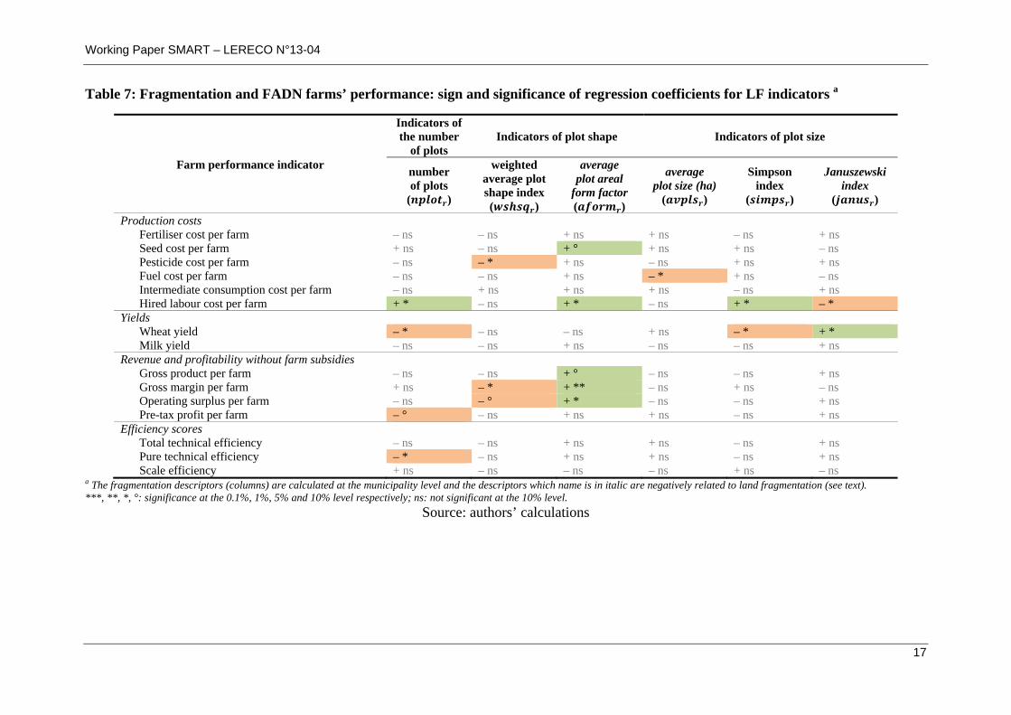
Due to space constraints, we do not present the detailed results for each of the 150

regressions. Instead, we report in Table 7 the signs and significance levels of the regression

coefficients obtained for each LF descriptor.


Table 7: Fragmentation and FADN farms’ performance: sign and significance of regression coefficients for LF indicators a

Farm performance indicator

Indicators of the number

of plots Indicators of plot shape Indicators of plot size

number of plots

( )

weighted average plot shape index ( )

average plot areal

form factor ( )

average plot size (ha)

( )

Simpson index

( )

Januszewski index

( )

Production costs Fertiliser cost per farm – ns – ns + ns + ns – ns + ns Seed cost per farm + ns – ns + ° + ns + ns – ns Pesticide cost per farm – ns – * + ns – ns + ns + ns Fuel cost per farm – ns – ns + ns – * + ns – ns Intermediate consumption cost per farm – ns + ns + ns + ns – ns + ns Hired labour cost per farm + * – ns + * – ns + * – *Yields Wheat yield – * – ns – ns + ns – * + * Milk yield – ns – ns + ns – ns – ns + ns Revenue and profitability without farm subsidies Gross product per farm – ns – ns + ° – ns – ns + ns Gross margin per farm + ns – * + ** – ns + ns – ns Operating surplus per farm – ns – ° + * – ns – ns + ns Pre-tax profit per farm – ° – ns + ns + ns – ns + ns Efficiency scores Total technical efficiency – ns – ns + ns + ns – ns + ns Pure technical efficiency – * – ns + ns + ns – ns + ns Scale efficiency + ns – ns – ns – ns + ns – ns

a The fragmentation descriptors (columns) are calculated at the municipality level and the descriptors which name is in italic are negatively related to land fragmentation (see text). ***, **, *, °: significance at the 0.1%, 1%, 5% and 10% level respectively; ns: not significant at the 10% level.


17


18

Table 7 (continued): Fragmentation descriptors and FADN farms’ performance: sign and significance of regression coefficients for LF

indicators a

Farm performance indicator

Indicators of plots’ distance from the farm Indicators of plots’ scattering

average distance of a hectare ( )

grouping index ( )

struc index tural ( )

Normalised av. nearest neighbour

distance ( )

Production costs Fertiliser cost per farm – ns – ns + ns – ns Seed cost per farm + ns – ns – ns – ns Pesticide cost per farm – ns – ns + ns + ns Fuel cost per farm – ns + ** + * + ns Intermediate consumption cost per farm + ns + ns – ns + ns Hired labour cost per farm + ° + ns + ns – ns Yields Wheat yield – ° – * – * + ns Milk yield – ns – ** – * + nsRevenue and profitability without farm subsidies Gross product per farm + ns + ns – ns + ns Gross margin per farm – ns + ns + ns + ° Operating surplus per farm – ns + ns + ° + ns Pre-tax profit per farm – * – ° + ns + ns Efficiency scores Total technical efficiency – ns – ns + ns + ns Pure technical efficiency – ns – ns – ns + ** Scale efficiency – ns – ns + ns – °

a The fragmentation descriptors (columns) are calculated at the municipality level and the descriptors which name is in italic are negatively related to land fragmentation (see text). ***, **, *, °: significance at the 0.1%, 1%, 5% and 10% level respectively; ns: not significant at the 10% level.



Our results show that, from a methodological point of view, each LF descriptor relates to one

or more performance indicators but not to all of them and that, reciprocally, each performance

indicator is explained by one or more LF descriptors but not by all of them. This gives

confidence in our strategy of using a wide set of variables for both dimensions. LF descriptors

which are most related to farm performance appear to be, first, the grouping index ( )

and the average areal form factor ( ), and then the structural index ( ) and the

number of plots ( ). The number of plots proves to be the only LF descriptor which is

significantly related to at least one indicator in the four categories of farm performance which

we considered, but the significance levels are somewhat limited (never less than 5%). By

contrast, the average size of plots, although a traditionally used LF descriptor, seems to have a

limited impact on the various dimensions of farm performance, be it directly considered

( ) or indirectly through the more elaborate indexes ( and ).

Most results regarding the detailed links between LF descriptors and performance indicators

conform to agronomic and economic intuition. Firstly, production costs are positively related

to the number of plots and to their distance from the farm, but decrease with plot size. The

results regarding the shape of plots are more surprising since they first suggest that seed cost,

pesticide cost and hired labour cost should decrease when plots are more irregularly shaped.

The result regarding seed cost is difficult to interpret but it is significant at the 10% level only.

However, the other two results, which are more significant, may be explained as follows: on

the one hand, irregularly shaped plots may impede the spread of pest attacks and hence reduce

the use and therefore cost of pesticides; on the other hand, irregularly shaped plots may be

more difficult to entrust to the care of hired, often less qualified, people so that the operator

will farm them himself or herself, hence reducing the cost of hired labour. Secondly, LF

appears to have a negative impact on yields, especially that of wheat, mostly through size and

distance. Thirdly, revenue and profitability are found to decrease with the number of plots, the

irregularity of their shape and their distance from the farm, but the average size of plots does

not seem to have a significant impact. Then again, counter-intuitive results (the positive

impact of on the operating surplus and of on the gross margin) are significant

at the 10% level only. Finally, total technical efficiency proves to be significantly related to

none of the considered LF descriptors. By contrast, conforming to intuition, the number of

plots seems to play a role in reducing pure technical efficiency, while the scattering of plots

affects scale efficiency. However, the positive and significant impact of the scattering of plots

on pure technical efficiency is more difficult to interpret.

19


20

In order to present the regression results in a more practical and vivid way, we simulated the

impact of a reduction in LF at the municipality level on two key performance indicators;

wheat yield, as a main physical component of farm performance, and pre-tax profit, as a main

financial component of farm performance. This reduction in LF could hypothetically be

reached by, for example, a consolidation programme. To this end, we computed for each LF

descriptor what improvements in pre-tax profit and wheat yield could be obtained by the

average farm when moving, at the municipality level, from one LF quartile to the next in the

direction of reducing fragmentation. With this, fragmentation improvements are immediately

readable in terms of Euros per farm for the pre-tax profit and tons per hectare for the wheat

yield. Therefore, this can illustrate the relative importance of LF descriptors whose estimated

regression coefficients are not directly comparable with each other.

Table 8 illustrates that the highest benefits in terms of pre-tax profit would be reached by

reducing LF in terms of distance of plots from the barycentre of the farm: on average,

decreasing the average distance of a hectare ( ) at the municipality level by around

500 m would raise the pre-tax profit by 5,862 Euros per farm – a 43% increase. By

comparison, reducing the average number of plots ( ) per farm at the municipality level

from 22.5 to 14.5 would lead to a pre-tax profit increase of 4,987 Euros per farm (or 37%).

Concerning the yield of wheat, the highest benefits (almost 0.5 ton per hectare, or a 9%

increase) would be obtained from a reduction in the grouping index ( ), i.e., by

reducing the maximum distance of plots from their barycentre, rather than their average

distance. In the case of the wheat yield, the second best option would consist of improving the

size of plots at the municipality level as measured by the Januszewski ( ) and the

Simpson ( ) indexes, rather than the number of plots by farms, with expected gains

estimated at approximately 0.4 ton per hectare (or an 8% increase).


Table 8: Pre-tax profit and wheat yield regression results and potential improvements for each land fragmentation descriptor a

Land fragmentation descriptor Regression estimate (std. dev.) Descriptor quartiles Improvement

Pre-tax profit Wheat yield Q1 Q3 Pre-tax profit (Euros per farm)

Wheat yield (tons per hectare)

Number of plots ( ) -629.51 (360.50)°

-0.041 (0.019)*

14.56 22.49 4,986.75 (2,855,75)°

0.323 (0.154)*

Weighted average plot shape index ( ) -36,276.57 (35,861.91)

-0.893 (1.446)

1.301 1.378 2,767.93 (2,736.29)

0.068 (0.110)

Average plot areal form factor ( ) 1,529,747 (1,123,538)

-28.749 (46.887)

0.042 0.045 3,816.72 (2,803.23)

-0.072 (0.117)

Average plots’ size ( ) 77.29 (1,043.45)

0.060 (0.064)

3.63 5.84 171.37 (2,313.60)

0.132 (0.142)

Simpson index ( ) -56,885.52 (52,879.09)

-6.851 (2.886)*

0.815 0.871 3,176.96 (2,953.21)

0.384 (0.161)*

Januszewski index ( ) 73,543.39 (47,487.62)

6.692 (2.666)*

0.271 0.333 4,548.27 (2,936.86)

0.414 (0.165)*

Average distance of a hectare ( ) -11.54 (5.83)*

-0.00058 (0.00030)°

1,369 1,877 5,861.69 (2,960.35)*

0.297 (0.153)°

Grouping index ( ) -1,615.90 (929.33)°

-0.145 (0.065)*

7.686 11.009 5,369.48 (3,088.08)°

0.481 (0.215)*

Structural index ( ) 337.84 (880.19)

-0.277 (0.117)*

1.803 3.384 -534.08 (1,391.44)

0.439 (0.185)*

Normalised average nearest neighbour distance ( 5,506.71 (8,334.41)

0.082 (0.369)

0.803 1.121 -1,753.17 (2,653.42)

-0.026 (0.118)

a For each LF descriptor, the ‘improvement’ (two last columns) represents what, for the average farm, would be the impact on the pre-tax profit and the wheat yield of a reduction in the fragmentation of the municipality, obtained by moving from one quartile to the other (columns four and five) given the estimated regression coefficients (second and third columns); as it is reported as an ‘improvement’, the impact corresponds to moving from Q3 to Q1 for descriptors positively related to land fragmentation and from Q1 to Q3 for those negatively related (see text for further details). ***, **, *, °: significance at the 0.1%, 1%, 5% and 10% level, respectively.


21


Such figures may look quite substantial for both performance indicators. However, they are

mainly intended to illustrate our results and especially to compare the marginal benefit (or,

reciprocally, the relative burden) of each LF dimension on the various aspects of performance.

They should not be viewed as accurate predictions, for at least three reasons. Firstly, the

simulated LF improvements may actually be very substantial themselves, hence very costly to

implement in real life. Thus these implementation costs should be compared, in addition to

comparing the benefits from improving one LF descriptor with respect to the others.

Secondly, it is hardly plausible that a particular consolidation programme would enhance one

LF descriptor only, leaving the others unchanged. In general, a consolidation programme

would seek to improve several LF dimensions at the same time, e.g., by reducing the number

and distance of plots, improving their shapes and increasing their average size. However,

these dimensions may be competing among themselves to some extent, so that a compromise

would have to be reached, leading to a limited improvement in each dimension – if not to a

deterioration for some descriptors in some cases. It is our view that the way in which these

multi-dimensional benefits and costs aggregate together remains an empirical question, which

may be addressed only thanks to hypothetical simulations such as that of Gonzalez et al.

(2007) or for specific case studies. Thirdly, the above average pre-tax profit and wheat yield

improvements may also reveal that such heavy consolidation programmes are likely to induce

additional changes in farming practices and in farm production, so that they should not be

simply compared to the average pre-consolidation figures as if they were ceteris paribus.

4 Conclusion

We have investigated the relationship between agricultural land fragmentation (LF) and farm

performance in 2007 in the French NUTS2 region of Brittany. Various farm performance

indicators (in terms of costs, yields, revenue, profitability, technical and scale efficiency)

calculated for a sub-sample of FADN farms were regressed on several explanatory variables,

including average LF descriptors computed for the municipalities where those farms were

located. Among the LF descriptors used, we considered not only the number of plots and the

mean size of plots which are traditionally used in the economic literature investigating the

impact of LF on farm performance, but also more complex indexes, in order to account for:

the shape of plots; (a proxy of) the distance between plots and farmsteads; and the distance

between plots themselves (or scattering of plots).

22


In our view, our analysis highlights that, from a methodological perspective, the measures of

LF traditionally used in the literature, namely the number of plots and the average plot size,

may not reveal the full set of significant relationships with farm performance because they do

not capture all the dimensions of land fragmentation. In particular, they exclude distance

considerations. In this respect, the grouping index used here seems to be powerful. However,

circumventing the absence of information regarding the location of the farmsteads by

computing distances relative to the farm barycentre, as we have done in this paper, may

introduce some bias that would be worth investigating.

Considering only the significant relationships, the analysis of farm performance and LF gives

three main findings. Firstly, whatever the LF descriptor considered, in general similar

conclusions are reached regarding the impact of LF on the various components of farm

performance. There are three main conclusions: i) LF tends to increase production costs; ii)

LF has a negative impact on crop yields; iii) LF tends to reduce the revenue and profitability

of the farm. Such findings that LF is overall harmful to farm performance are consistent with

those found in the previous literature on the subject. Secondly, these very general conclusions

should not hide the fact that in some cases, even if very few, the impact of LF on farm

performance was the opposite to that expected, and that it was not always possible to find an

economic rationale for such results. This is another argument in favour of using several LF

indicators to investigate the link between fragmentation and performance. Thirdly, we have

shown that the benefits from reducing fragmentation may differ with respect to the improved

LF dimension and the performance indicator considered. The overall impact of a real-life

consolidation programme, which may modify several LF dimensions at the same time,

remains an empirical open question which should be investigated carefully in each specific

case.

We should also stress that, while the general finding of our analysis is a negative impact of LF

on farm performance, we do not advocate a ‘blind’ reduction of farm fragmentation through

large scale and systematic consolidation programmes. One reason is the necessity of

balancing the private and societal gains of LF reduction. In the Brittany case, fragmented

agricultural land is usually associated with hedges and natural corridors which have been

shown to be beneficial to, e.g., biodiversity, water fluxes and the environment in general

(Thenail and Baudry, 2004; Thenail et al., 2009). This indicates that the private costs of LF at

the farm level should be carefully balanced with potential public benefits at society’s level. In

this respect, programmes which aim at enhancing the structure of field patterns under the

23


constraint of preserving and/or replanting hedges, such as the ‘amicable plot exchange’

programme put in place in Brittany by the agricultural extension services and the local

authorities, may represent an efficient compromise (CA Bretagne, 2011).

Even though these results sound reasonable and generally conform to intuition, our analysis

suffers two major limitations which should be considered with great care if such research is to

be aimed at proposing a consolidation programme. Firstly, endogeneity issues would have to

be investigated carefully: although we can be relatively confident that the relationship

between variables is mainly in one direction from a static point of view, namely that

municipalities’ LF influences the performance of specific farms, it might be that, in a dynamic

perspective, efficient farms are more likely to be in a position to decrease their fragmentation

at the expense of neighbouring farms. Secondly, drawing any causal conclusions would mean

assuming a direct link between the LF of the municipality where the considered farm is

located, and the LF within the farm itself: though the approach adopted here – due to data

limitations – indeed relies on the hypothesis that the higher the LF of the municipality, the

higher the probability for the farm to be fragmented, it may happen that farms which are not

very fragmented may be located in a highly fragmented municipality, and vice versa. Finding

a way to gain access to a measure of fragmentation at the individual level for the farms in our

sample constitutes a major challenge for future work. Although our analysis has shed some

light on the relationship between the performance of a farm and the LF in the municipality

where it is located, further investigation is therefore needed, especially before any policy

recommendations can be made.

24


References

Akkaya Aslan, S.T., Gundogdu, K.S., Arici, I. (2007). Some metric indices for the assessment

of land consolidation projects. Pakistan Journal of Biological Sciences 10:1390-1397.

Blarel, B., Hazell, P., Place, F., Quiggin J. (1992). The economics of farm fragmentation:

evidence from Ghana and Rwanda. The World Bank Economic Review 6:233-254.

CA Bretagne (2011). Guide pratique : J’échange mes parcelles pour gagner. Chambres

d’Agriculture Bretagne, Rennes (France), 26 p.

Charnes, A., Cooper, W., Rhodes, E. (1978). Measuring the efficiency of decision making

units. European Journal of Operational Research 2:429-444.

Del Corral, J., Perez, J.A., Roibas, D. (2011). The impact of land fragmentation on milk

production. Journal of Dairy Science 94:517-525.

Di Falco, S., Penov, I., Aleksiev, A., Van Rensburg, T. (2010). Agrobiodiversity, farm profits

and land fragmentation: Evidence from Bulgaria. Land Use Policy 27:763-771.

European Commission (2000). Council Regulation (EC) No 1593/2000 of 17 July 2000

amending Regulation (EEC) No 3508/92 establishing an integrated administration and

control system for certain Community aid schemes. Official Journal L182:0004-0007.

European Commission (2010). Farm Accounting Data Network – An A to Z of Methodology.

Version 04/10/2010, http://ec.europa.eu/agriculture/rica//pdf/site_en.pdf (last accessed

04.02.2013).

Gonzalez, X., Alvarez, C., Crecente, R. (2004). Evaluation of land distributions with joint

regard to plot size and shape. Agricultural Systems 82:31-43.

Gonzalez, X., Marey, M., Álvarez, C. (2007). Evaluation of productive rural land patterns

with joint regard to the size, shape and dispersion of plots. Agricultural Systems 92:52-62.

Hung, P.V., MacAulay, T.G., Marsh, S.P. (2007). The economics of land fragmentation in the

north of Vietnam. Australian Journal of Agricultural and Resource Economics 51:195-

211.

Jabarin, A.S., Epplin, F.M. (1994). Impacts of land fragmentation on the cost of producing

wheat in the rain-fed region of northern Jordan. Agricultural Economics 11:191-196.

Kawasaki, K. (2010). The costs and benefits of land fragmentation of rice farms in Japan.

Australian Journal of Agricultural and Resource Economics 54:509-526.

25


26

King, R., Burton, S. (1982). Land fragmentation: notes on a fundamental rural spatial

problem. Progress in Human Geography 6(4): 475-494.

Manjunatha, A., Anik, A.R., Speelman, S., Nuppenau, E. (2013). Impact of land

fragmentation, farm size, land ownership and crop diversity on profit and efficiency of

irrigated farms in India. Land Use Policy 31:397-405.

Marie, M. (2009). Des pratiques des agriculteurs à la production de paysage de bocage. Étude

comparée des dynamiques et des logiques d’organisation spatiale des systèmes agricoles

laitiers en Europe (Basse-Normandie, Galice, Sud de l’Angleterre). Ph-D dissertation of

the University of Caen/Basse-Normandie, Caen (France), 513 p.

Nguyen, T., Cheng, E., Findlay, C. (1996). Land fragmentation and farm productivity in

China in the 1990s. China Economic Review 7:169-180.

Parikh, A., Shah, K. (1994). Measurement of technical efficiency in the northwest frontier

province of Pakistan. Journal of Agricultural Economics 45(1):132-138.

Rahman, S., Rahman, M. (2008). Impact of land fragmentation and resource ownership on

productivity and efficiency: The case of rice producers in Bangladesh. Land Use Policy

26:95-103.

Tan, S., Heerink, N., Kuyvenhoven, A., Qu, F. (2010). Impact of land fragmentation on rice

producers’ technical efficiency in South-East China. NJAS - Wageningen Journal of Life

Sciences 57:117-123.

Thenail, C., Baudry, J. (2004). Variation of farm spatial land use pattern according to the

structure of the hedgerow network (bocage) landscape: a case study in northeast Brittany.

Agricultural, Ecosystems and Environment 101:53-72.

Thenail, C., Joannon, A., Capitaine, M., Souchère, V., Mignolet, C., Schermann, N., Di

Pietro, F., Pons, Y., Gaucherel, C., Viaud, V., Baudry, J. (2009). The contribution of crop-

rotation organization in farms to crop-mosaic patterning at local landscape scales.

Agricultural, Ecosystems and Environment 131:207-219.

Wan, G., Cheng, E. (2001). Effects of land fragmentation and returns to scale in the Chinese

farming sector. Applied Economics 33(2):183-194.

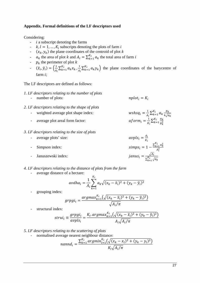
Appendix. Formal definitions of the LF descriptors used

Conside grin : ript de

- … , subscripts denoting the plots of farm - s noting the farms a ubsc

, 1, - , the plane c ord e o ntroid of plot in

-

o at s f the ce- f lot a d ∑ he total area of farm the area o p n t

the perimeter of plot - , ∑ , ∑ the plane coordinates of the barycentre of

farm ; The LF descriptors are defined as follows: 1. LF descriptors relating to the number of plots

- number of plots:

∑2. LF descriptors relating to the shape of plots

- weighted average plot shape index:

- average plot areal form factor: ∑

3. LF descriptors relating to the size of plots

- average plots’ size:

- Simpson index: 1∑

- Januszewski index: ∑

4. LF descriptors relating to the distance of plots from the farm

- average distance of a hectare:

1

- grouping index:

⁄

- structural index: .

⁄

5. LF descriptors relating to the s tter otsca ing of pl

- normalised average nearest neighbour distance: ∑

⁄

27


Les Working Papers SMART – LERECO sont produits par l’UMR SMART et l’UR LERECO

• UMR SMART L’Unité Mixte de Recherche (UMR 1302) Structures et Marchés Agricoles, Ressources et Territoires comprend l’unité de recherche d’Economie et Sociologie Rurales de l’INRA de Rennes et les membres de l’UP Rennes du département d’Economie Gestion Société d’Agrocampus Ouest. Adresse : UMR SMART - INRA, 4 allée Bobierre, CS 61103, 35011 Rennes cedex UMR SMART - Agrocampus, 65 rue de Saint Brieuc, CS 84215, 35042 Rennes cedex

• LERECO Unité de Recherche Laboratoire d’Etudes et de Recherches en Economie Adresse : LERECO, INRA, Rue de la Géraudière, BP 71627 44316 Nantes Cedex 03 Site internet commun : http://www.rennes.inra.fr/smart/

Liste complète des Working Papers SMART – LERECO : http://www.rennes.inra.fr/smart/Working-Papers-Smart-Lereco

http://econpapers.repec.org/paper/raewpaper/

The Working Papers SMART – LERECO are produced by UMR SMART and UR LERECO

• UMR SMART The « Mixed Unit of Research » (UMR1302) Structures and Markets in Agriculture, Resources and Territories, is composed of the research unit of Rural Economics and Sociology of INRA Rennes and of the members of the Agrocampus Ouest’s Department of Economics Management Society who are located in Rennes. Address: UMR SMART - INRA, 4 allée Bobierre, CS 61103, 35011 Rennes cedex, France UMR SMART - Agrocampus, 65 rue de Saint Brieuc, CS 84215, 35042 Rennes cedex, France

• LERECO Research Unit Economic Studies and Research Lab Address: LERECO, INRA, Rue de la Géraudière, BP 71627 44316 Nantes Cedex 03, France Common website: http://www.rennes.inra.fr/smart_eng

Full list of the Working Papers SMART – LERECO:

http://www.rennes.inra.fr/smart_eng/Working-Papers-Smart-Lereco http://econpapers.repec.org/paper/raewpaper/

Contact Working Papers SMART – LERECO INRA, UMR SMART 4 allée Adolphe Bobierre, CS 61103 35011 Rennes cedex, France Email : [email protected]

http://www.rennes.inra.fr/smart/

mailto:[email protected]


2013

Working Papers SMART – LERECO

UMR INRA-Agrocampus Ouest SMART (Structures et Marchés Agricoles, Ressources et Territoires)

UR INRA LERECO (Laboratoires d’Etudes et de Recherches en Economie)

Rennes, France

does land fragmentation affect farm performance? a …ageconsearch.umn.edu/bitstream/207854/2/wp...

Documents