FAMILIES OF ESTMATOR-BASED STOCHASTIC

LEARNING ALGORITHMS

by

M A R N A AGACHE, BSc.

A thesis submitted to the

Fsculty of Graduate Stuâies and Research

in partial fulfdment of the requhrnents for the degree of

Master of Computer Science

Ottawa-Carleton Institute foi Computer Science

School of Computer Science

Carleton University

Ottawa, Ontario

Jdnuary 2000

O copyright

2 0 , Mariana Agache

9 uisiîions and Acquisitions et Bib iognphic Setvices senrices bibliographiques

The author has granted a non- L'auteur a accordé une licence non exclusive licence allowing the exclusive permettant à la National Libraxy of Canada to Bibliothèque nationale du Canada de reproduce, loan, distn'bute or sel1 reproduire, prêter, distribuer ou copies of this thesis in microfonn, vendre des copies de cette thèse sous paper or electronic formats. la forme de microfiche/nlm, de

reproduction sur papier ou sur format électronique.

The author retahs ownership of the L'auteur conserve la propriété du copyright in this thesis. Neither the droit d'auteur qui protège cette thèse. thesis nor subsmntial extracts fkom it Ni la thèse ni des extraits substantiels may be printed or othe~wise de celle-ci ne doivent être imprimés reproduced without the author's ou autrement reproduits sans son permission. autorisation.

This thesis studies the field of Estimator-based Leamhg Automata. We fust

argue that the Reward-Penalty and Reward-Inaction learning paradigms in conjunction

with the continuous and discrete models of computation lead to four versions of Pursuit

Leamhg Automata. Such schemes permit the Learning Automaton to utilize the long-

terni and short-term perspectives of the environment. We present al1 four resultant

Pursuit algorithrns, and a quantitative cornparison of their performance.

The existing Rirsuit Algorithms 'pursue' the action that is cumntly estimated as

the k t action. In this thesis. we claim that by punuhg al l the actions with higher

estimates than the chosen action, the perîormance of the Pursuit Aigorithm improves

considerably. To attest this, we introduce two new Pursuit algorithms, and justify their

supenonty through extensive simulations.

Thathachar and Sastry introduced the TSE estimator algorithm and pnsented its

updating equations in a scalar fom. in this thesis. we present a vectorial representation

of the TSE algorithm. and propose its generalized vectorial version. whose superiority is

aiso p m n experimentaiiy.

First and fonmost, 1 would iike to thank my Professor. Dr. John Oommen, for bis

continuous support, encouragement, and for believing in me. Throughout these years, his

guidance. ideas, and enthusiasm gave me the opportunity to explore new scientific

domains and to discover new ~ c a r c h horizons, for which 1 am deeply gratehil.

1 wodd also Like to thank Professor M. A. L. Thathachar, of the Indian Institute of

Science, Bangalore, India, for his valuable comments and suggestions related to the work

presented in the Chapter 3 of this thesis.

1 would like to thank my parents, my sister and Wellington for their help, support,

and encouragement.

To my parents.

CEMPIBR 1: INTRODUCTION . r a a t m . . m m m m ~ m ~ m m m m ~ . m m m m ~ . m m m m m m m m m m m m a m m m m m m m m m m m m m m m m m m m o m m m m m m a 1

1 .1 General description of the leamhg automata ...... .. . . ... ..... ...... .... .. .. . . . . . 1

1.2 Justification and objectives of the Thesis .............. ... ..... ... .... + . . . .............. 6

1.3 Contributions of the Thesis ............................ .*.......CIC ....... .........................*..*.......... 7

1.4 Content and organization of the Thesis ................... .e.e.~....e~.......~............................ 9

CI~APTER 2 t L ~ G AUTOMATAIAN O ~ V W ..m.mma~.smmmmmmmmmmmmmw.aaommmaa.t...aoomommoo 11

2-1 Definition of Automaton ....,.. ... .................*........+.. .. ..... , ... . . ........ .........1 1

2.1.1 Determiaistic Automaton ........,..... , .... ,.......e......,.........*...*..................**..... 12

2.1.2 Stochastic Automaton ..................................... .-...... .................................. 13

vi

2.2 The Leaming Automaton .................................. ..................................................... 15

.............................................................. ............ 2.2.1 The Environment ..... .... 1 6

2.2.2 Defdtion of the Learning Automaton ................... .. ................................... 17

2.2.3 N o m of behavior ...................... ...................................................................... 18

2.3 Fied Structure and Variable Structure Leaming Automata ........... ................... ... 21

2.3.1 Fixed Stmcture Automata ....................................................................... 21

2.3.1.1 Tsetlin Automaton ................ .. ................................................................ 21

2.3.1.2 Krinsky Automaton ...................... .... ................. ................................ 24

.................................... .. ........ ...... 2.3.1.3 Krylov Automaton ...... .. ... .... 26

2.3.2 Variable Structure Stochastic Automata ...................................................... 2 7

2.3.2.1 Linear Reward-Penalty Scheme (LRp) .............. ..... .............. ................. 31

2.3.2.2 Linear Reward-Inaction Scheme (LR3 ..................................................... 32

2.3.2.3 b a r Inaction-Penalty Scheme (La) ............................. ........ ................ 33

2.3 -3 Discniwd Leaming Automat a. .......... ..... .. ...... ...... 2.3.3.1 Discreiized Linear Reward-Inaction Automaton ................................ 35

.................. ............. 2.3.3.2 Discretized Linear Inaction-Penalty Automaton .. 3 8

.................. .................. 2.3.3.3 Discreiized Linear Reward-Penalty Automaton .... 39

2.4 Estirnator Algor i th ..................................................................... d 2.4.1 Overview ...................... .. ...... ........- 2.4.2 Continuous Estimator Algorithms .................................................................... 45

2.4.2.1 Pursuit Algorithm ...................... .. ....... ............................m....-............ ..45

2.4.2.2 TSE Algorithm ..................... ................................. ................................ 47

vii

2.4.3 Discrete Estimator Algorithm ......................................................................... 5 1

2.4.3.1 Discrete Pursuit Algorithm ........... .. .... .. ....................................... 5 2

24.32 Discnte TSE Algorithm .............................. ............................ .. ............ 54

2.5 Conclusions ................... .......................... ...................... 5 8

CHAITER 3: NEW PURSUIT ALGORX'RXMS O O O O O O O ~ O ~ O ~ ~ O ~ O O O . O ~ O O H O O ~ O O ~ O ~ ~ O O H H O ~ ~ ~ ~ O ~ ~ H O O O W H H ~ O ~ ~ ~ 60

.................................... 3.1 introduction ........ ............................................................. 60

3.2 Continuous Reward-inaction Rusuit Algorithm (CPR J ................................. 62

3.3 Discntized reward-penalty h u i t Algorithm (DPRP) .... .................... .............. 66

...................... 3.4 Simulation Resuits .. ........ ............................................... .......... 69

3.5 Conclusions ............................................................................................................. 75

CHAPTER 4: GENEWIZATION OF THE PURSUIT ALGORITHM ~ 0 ~ ~ 8 0 0 0 0 ~ 0 0 0 0 0 0 ~ 0 0 ~ 8 0 ~ 0 ~ 8 0 0 0 0 0 0 ~ 0 0 8 77

4.1 Introduction ............... ........................ ................................................................. 77

4.2 Generaiizeù Rumit Algorithm .......................................................................... 8 0

4.3 Discretized Generalized Pursuit Algorithm ................... .. ............. ................. 86

4.4 Simulation Results .............. .............. .................... .. ............................................................................... 4.5 Conclusions 93

CHAFM3R 5: GENERALIZATION OF THE TSE A L c 0 ~ m r i l i o . o e w w e m e w ..8*e.*eSee**eHeeCeO*..***.e m. 94

5.1 Vectorial representation of the TSE algorithm .................................................... 94

5.2 ûeneralization of the TSE algorithm ...................... ....... ........................... 98

5.3 Simulation Results .................................... ......................................................... 105

........................................................................................................... 5.4 Conclusions 1 0

viii

6: CONCLUSIONS b b m m b b o ~ b o b b b m b b b b b b ~ ~ b b O ~ ~ b b b m m w m ~ m o O b b m m b b m o b b m o m m m b . o m ~ b b b b b o o o o ~ ~ m ~ o b ~ ~ b m o O ~ o 111

6.1 Summary ............................... ....................................................................... 1 1 i

6.2 Future work ........................................................,.....................~.................~.......~.. L 15

LIST OF TABLES

Table 2.1: Experimental comparative performance of DLRi with other FSS A [ 141. ...... 38

Table 2.2: Comparative performance of DLRi. ADLp, ADLW (c2a.8) ....................... 4 1

Table 2.3: Comparison between continuous and discrete linear VSSA ......................... 42

Table 2.4: The number of iterations until convergence in two-action environments for

the TSE Algorithm [IO] ........................................................ .... *-...-...* .......... 56

Tabk 2.5: Comparison of the discrete and continuous estimator dgoritbms in

benchmark ten-action environments [ 10 1. ............... ................ ....... . . . . 5 7

Table 3.1: Comparison of the Pursuit algonthms in two-action benchmark environments

for which exact convergence was requi~d in 750 experiments (NE=750). .7 1

Table 32: Comparison of the Pursuit algorithms in two-action benchmark envhnrnents

for which exact convergence was required in 500 experiments (NE=Sûû). .7 1

Table 3.3: Comparison of the Rirsuit algonthms in new two-action environments for

which exact convergence was required in 750 experiments -750) ........ 73

Table 3.4: Cornpanson of the Pursuit algorithms in ten-action benchmark environments

for which exact convergence was required in 750 experiments -750). .74

Table 33: Comparison of the h u i t algorithms in ten-action benchmark environments

for which exact convergence was nquired in 500 experiments (NErSOO). .74

X

Tabk 4.1 : Performance of the generalized Pursui t algorîthms in benchmark ten-ac tion

environments for which exact convergence was required in 750 experiments

-750) .. .....r........ir....o...................................-..................................~o..-.. 91

Table 5.1: Performance of the GTSE and TSE algorithms in ten-action benchmark

enviroaments for which exact convergence was requhd in 750 experiments

(NE=750) ................... .... ................................................................. 106

Table 5.2: Performance of the GTSE and DTSE algorithms in benchmark ten-action

environments for which exact convergence was required in 750 experiments

(NE=750) .................. .,...., ....................................................................... 109

Fipre 2.1:

Figure 2.2:

Figure 2.3:

Figure 2.4:

Figure 2.5:

Figure 2.6:

Figure 3.1:

Figure 4.1:

Fipre 4.2:

Figure 5.1:

The automaton. .... ...... .... ..... .... . ........ ............................. . . . . . . . 1 1

The environment ..... . ........ ........., ... . . .............. . . . . ......... . 1 6

Feedback connection of automaton and environment. ...............-.. .... ... .. ..... 17

State transition graphs for the Tsetîin automaton LzN2 ................... ............ 22

State transition graphs for the Krinsky automaton K ~ ~ ~ , ~ ....... . .................... 25

State transition graphs for the Krylov automaion K ~ ~ , ~ ............... ........ .... ..26

Cornphson of the Punuit algonthms in two-action benchmark

environments for which exact convergence was required in 750 experiments

(NE=750). ............................................................*.........* .... ....b...... ......... ...72

Solution approach of the CPRp Pursuit Algorithm and the Generalized

Pursuit algonthms ........ ................ ... ... .......... ...................... . . . . . . 7 8

Performance of the Pursuit Algorithm relative to the CPRp algonthm in ten-

action environments for or which exact convergence was required in 750

experiments ..................................... . . . . ............. . b........................b... 92

Performance of the continuous Estimator Algorithrns relative to the CPRp

aigorithm in ten-action environments for or which exact convergence was

. * requlzed m 750 experiments ............ ... ..... ............................ . ......107

Figure 6.1: Performance of some Estimator Aîgorithms relative to the CPRp algorithm

in ten-action enviroments for which exact convergence was required in 750

experiments ................... .... .................. . ....... . .............. ........ 1 14

Chapter 1: INTRODUCTION

1.1 General description of the learning automata

Learning represents one of the most important psychological processes and it is

essential in the behavior of self-adjusting organisms. In psychology. it can be defined as

an organism's ability to modify its current behavior based on past behavior and the

consequences of its pnor cboices. The psychological and bioiogicai concepts of leaming

have been widely studied and have been incorporated in many engineering systems that

deal with incomplete information and uncertainty. Applications such as Adaptive

Control Systems. Pattern Recognition. Game Theory, and Objeci Panitioning, needed to

incorporate leaming characteristics in their huictionality in order to mode1 systerns with a

substnntial amount of uncertainty. Many of these systems are required to choose the

correct action (decisions) without a priori knowledge of the consequences of perfonning

these actions. To perform well under these conditions of uncertainty, the systems needed

to acquire some knowledge about the consequences of performing the various actions

This acquisition and utiluation of relevant knowledge in order to improve the

performance of a system is posed as the learning problem. 'ïhe goal of the learning

problem is to compensate for the insuffient infornation by appropriate data collection 1

and processing, while moving the process towards its solution. In these engineering

systems, leming has been implemented using various methods and techniques, namely:

stochastic approximation methods] [3], heuristic programmuig techniques [23], inductive

Uiferential techniques 1251, and statisticai infenntial techniques [4] [SI.

Another approach to solving the leaming problem was initiated by the Russian

mathematician Tsetlin. He introduced, in 196 1, a new mode1 of computer learning that is

now cailed a lraning automaton. and which wili be the focus of the study presented in

this thesis. The goal of such an automaton is to determine the optimal action out of a set

of dlowable actions. The functionality of the leaming automaton cm be described in

terms of a sequence of npetitive feedback cycles in which the automaton interacts with

an Environment. The automaton chooses an action that triggers a response from the

Environment. Such a response cm be either a reward or a penaity. The automaton uses

this response and the knowledge acquired in the p s t actions to determine which is the

next action. The term Environnent refers, in general. to the collection of al1 extemal

conditions and influences affecting the life and development of an organism or system.

In the context of leaming automata, the ierm defines a random unknown 'media' in

which an automaton or a group of automata can operate.

Learning automata can operate individually or c m be interco~ected in a

hierarcbicd or distributed fashion [30]. Some of the applications using leamhg automata

that operate in such diffennt organizational models are: telephone and traffic routing and

control [13], game theory [30]. stoc hastic geornetric problems [15], pattern recognition

[30], and the stochastic point location problem [20].

Leaniing automata can be classified with respect to their transition states as king

either detenninistic or stochastic. For a detednistic automaton, given an initiai state

and input, the next state and action are uniquely specified. For a stochastic automaton,

given an initial state and input sequence, there is no certainty r e g d n g the next states

and actions of the automaton. These automata can m e r be classified with respect to

their transition functions in iwo categories: Fked Structure Stochastic Automata (FSSA)

and Variable Structure Stochastic Automata (VSSA). In the case of FSSA, the state

transition and output functions are independent of time. and are thus considend to be of a

'îixed structure". The VSSA are designed with more flexibility, allowing the state

transition and output function to Vary in time.

The earlier models of stochastic leaming automata coasider the probability space

as a continuous space, the action probabilities king able to take any value in the interval

[O, 11. ui 1979, Thathachar and Oornmen [26] opened a new direction in the evolution of

the field of leamhg automata by introducing the concept of discretized leaniing

automuta. These automata operate in the probability space [O,l], which is divided into a

finite nurnber of continuous subintervals, and the probabilities of choosing different

actions an ailowed to assume values bom this finite set. The leaming automata designed

using this technique exhibit a decrease in their convergence tirne. The are therefore faster

than the leaming automata designed to use a continuous probabiiity space.

In the attempt to mode1 the psychological concepts of Ieaniing, various VSSA

usai different leaming paradip . Specifically, the basic concepts of the operant

conditioning leaming method have been applied in the context of the VSSA algorithrns.

These algorithms would update the action probabilities in the following situations: a)

wben the environment rewarded or penalized an action, b) when the environment

rewarded an action, ignoring the penalties, c) when the environment penalized an action,

ignoring the rewards.

In the quest to design even faster converging leaming algorithms, Thathachar and

Sastry [27] introduced a new class of learning automata, called estimator algorithms.

T h e aigorithrns are cbaracterized by the fact that they maintain running estimates for

the penalty probabüity of each possible action, and use hem to update the probabilities of

chwsîng each action. Thathachar and Sastry introduced the concepts of the estimator

algorithrns by F i t presenting the Pursuit Estimator Algorithm [27]. This leaming

aigorithm 'pursues' the action that is considered to have the highest reward estimate.

Later, in 1984, the same authon presented another estimator dgonthm, the TSE

aigorithm. wbich increases the action probabilities for al1 the actions that have higher

reward estirnates than the current chosen action. Oommen and Lanct6t continued the

study of the estimator algorithms and presented in 1990 discntized versions of the

Punuit and TSE algorithm.

Leaming Automata can be used to solve other, mon general, leaming problems or

can be employed as basic l e d g elements of other leaming machines. For instance, the

resevch on LA directly influenced the trial-and-error thrcad of reinforcement leurning,

leading to modem reinforcement leaming research [24]. Due to their leaniing

phiiosophy, LA c m be employed in solving simplifïed reinforcement leaming problems.

Specificdy, Sutton and Barto in (241 showed how LM, LRP, and the Pursuit schemes cm

be used in solving evaluative feedback problems such as the n-armed bandit problem.

Because the LA leam to choose the optimal action h m a set of ailowable actions, the

structure proves to be impractical for solving the full reinforcement learning problem,

which has as goal to maximize the total amount of reward received over the long mn. A

method that solves the full reinforcement problem is the Q-leaming method, whose

objective is to find a control ruk that maximizes at each time step the expected

discounted sum of future reward. From this perspective. the LA differ from the Q-

leaming method because they attempt only to l e m the optimal action, independently of

the expected sum of rewards.

Narendra and Thathachar (1 I ] pnsented various models on interconnected

learning automata. such as synchronous and sequential modes, hierarchies and networks

of learning automata. The last mode1 of interconnected automata was strongly intluenced

by the multilayered artificial neural networks or co~ectionist networks, but with some

underlying diffennces. Specifically, the networks of leaming automata differ from the

neural network mode1 in the way the networks are adjusted. The neural networks are

adjusted based on the e m r between the output of the network and some desired output,

whenas the adjustment in the network of automata depends on the ranùom response from

the environment. In both cases. their performance fuactions are improved by the

adjustment of the weight vectors. Further cesearch is necessary in the field of L e d g

Automata to determine the weights of a leaming network using the learning automata

schemes.

1.2 Justitication and objectives of the Thesis

This thesis concentrates on the study of the estimator algorithms, focusing

primarily on the introduction of new and better-performing estimator algoriibms. It also

studies the characterization of their performance in cornparison to the existing estimator

algorithms.

The original Pursuit algorithm presented by Thûthachar and Sastry is a continuous

algorithm that updates the action probabili ties whenever the environment rewards and

penalizes an action. Oornmen and Lanctôt [18] Iater extended the Punuit algorithm into

the discntized world by presenting the Discretized Pursuit Algonthm based on the

reward-inaction learning paradigrn. The Reward-Penaity and Reward-Inaction leaming

paradigms in conjunction with the continuous and discrete models of computation leads

to four versions of Punuit Leaming Automata. but only two of hem have been presented

in the literature. This represents a gap in the class of the learning automata, which we

address. Hence, one of the objectives of this study is to introduce the new versions of

Pursuit algorithms that completely covers ail possible versions of these algorithms, and to

present a thorough cornparison of their performance based on simulation results.

The Pursuit algorithm 'pursues' the action that is cumntly estimated as the best

action. This implies that, if at a certain time in the evolution of the automaton, the action

that is estimated to be the best action is not the action with minimum penalty probability,

the automaton pursues a wroag action. This behavior of the automaton can considerably

increase its convergence t h e in such environments and we consider this as a limitation in

the design of Putsuit aigoriihms. Therefoce, another objective of this thesis is to impmve

the design of the Pursuit algorithm in order to minimize the probability of pursuing a

mong action, and to increase its convergence performance.

Oommen and Lanctôt [18] presented a continuous version of the Pursuit in a

vectoriai form, allowing for a better undentanding of the concepts of the hirsuit

dgorithrn. To better outline the underlying concepts of the TSE algorithm. a goal of our

study is to generate a vectorial fom of the TSE algorithm. and to propose new directions

of improvement of the performance of the TSE algorithm.

In sumrnary, the m i n objectives of this thesis are:

to ma te new Pursuit algorithms that utilize in their design the reward-penalty

and rew ard-inaction leamhg paradigms, and to stud y their performance:

to mate new Pursuit algorithms that minimize the probability of choosing a

wrong action. there fore exhibithg a better convergence performance;

to generate a vectotial representation of the updating equations of the TSE

aigorithm and to determine new directions of improving the performance of

the TSE algorithm.

13 Contributions of the T hesis

In this thesis, we htmduce five new estimator algorithms: the Continuous Pursuit

Reward-Inaction Algorithm (CPRd, the Discrete Pursuit Reward-Penalty Algorithm

@PRP), the Generalued Rusuit Algorithm (GPA), the Discretized Generalized Rirsuit

Algorithm (DGPA), and the Generaîized TSE Algorithm (GTSE).

The Continuous Pursuit Reward-inaction (CPRd and the Discrete Pursuit Reward-

Penalty (DPw) dgorithrns, dong with the existing Continuous hirsuit Reward-Penalty

(CPRP) and Discrete Pursuit Reward-Inaction @PRI) algorithms, completely cover al1 the

possible venions of hirsuit algorithms that use the Reward-Penalty and Reward-inaction

leaming paradigms. The experimental results obtained dunng this study prove that

among these algorithms, the DPRi is the fastest one. Furthemore, we have found that the

Reward-Inaction schemes are generdly supenor to their Reward-Penalty counterparts.

and we have experimentally verified that the discretized schemes exhibit a beiter

performance than the continuos schemes.

The search for a new direction of improving the performance of the Pursuit

algorithm led to the development of the generalized Pursuit algorithms GPA and DGPA.

These algorithms generaüze the concepts of the original Pursuit algorithm by puauing

more than one action, therefore minimizing the probability of pursuhg a wrong action

and increasing the performance of these dgorithms. The Generalized Pursuit Algorithm

(GPA) proves to be the fasiest continuous Pursuit aigorithm, and the Discretized

Generalized Pursuit Algonthm (DGPA) proves to be the fastest discretized Rusuit

algorithm and, more generally, the fastest Pursuit algorithm reported to date.

Another contribution of this thesis is the development of an original vectorial

representation of the updaîing equations of the TSE algorithm. Tbis vectonal

repcesentation open a new direction of generaüzing the TSE algorith, and leads to the

introduction of the novel GTSE algocithm. This new aîgorichm experimentally proves to

be the fastest coniinuous estimator algorithm reported to date.

Chaptcr 1: Iirrrto~uerio~ 9

AU the novel algorithms proposed in ihis thesis exhibit very g d convergence

properties. Also, aU of these algorithms have been proven hopfimal in any stationary

random environment.

1.4 Content and organiza tion of the Thesis

This thesis debuts with an overview of the field of learning automata in Chapter 2,

presenting frst the underlying mathematical models, and also describing the measures of

the performance of these algorithms, inciuding expediency, optimdity, E-optimality and

absolute expediency. Also, in this chapter we present the concepts of the Fixed Structure

and Variable Structure Stochastic Automata, along with various linear schemes that use

different learning updating pûndigms such as the reward-penalty, the reward-inaction

and the inaction-penalty, Moreover, the continuous and discntized models of leaming

automata are portrayed through the examples of various such learning schemes.

Chqter 3 addresses the fini objective of this thesis, and contains a study of the

Pursuit algorithms with respect to different leaming p d g m s such as reward-penalty

and reward-inaction. The novel work presented in this chapter was published in the

technical papa 1161.

Chnpter 4 presents two new generalued Rirsuit algorithms, along with a relative

cornparison of their performance. The work presented in this chapter addresses the

second objective of this thesis. which is to improve the performance of the h u i t

estimator algorithms by minllnizllig the probability of pursuing a wrong action.

Cbapter 1: ~ O W ~ O N 10

The vectorial representation of the updating equation of the TSE algorith is

presented in Chapter 5. together with a new generaüzed TSE algorithm and an evaluation

of its perfomûnce.

Chapter 6 concludes the thesis by pnsenting a summary of the results, and

outlining the main conclusions of this work.

Chapter 2: LEARNING AUTOMATA-& OVERVIEW

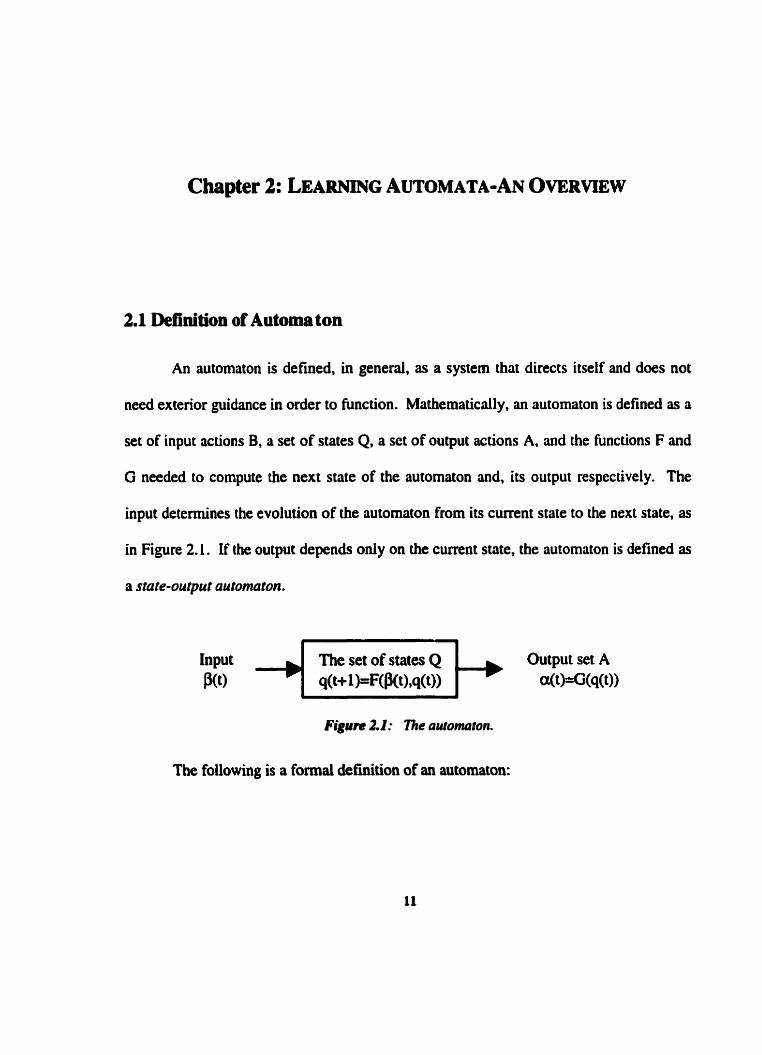
2.1 Definition of Automa ton

An automaton is defined, in general, as a system that directs itself and does not

need exterior guidance in order to function. Mathematically, an automaton is defined as a

set of input actions B, a set of states Q, a set of output actions A. and the hnctions F and

G needed to compute the next state of the automaton and, its output respectively. The

input determines the evolution of the automaton from its cwrent state to the next state, as

in Figure 2.1. If the output depends only on the cumnt state, the automaton is defined as

a state-output automatun.

Input The set of states Q Kt) q(t+l )=F(B(t),q(t))

Figurc 2.1: The automaton.

The following is a f m a l defullton of an automaton:

Chapter 2: L E A ~ ~ N ~ N G AUTOMATA - AN OV~RVIEW l2

Iklinition 2.1: An automaton is a quintuple <A,B,Q,F,G> , where:

A={al. a2,. . .,el is the set of output actions of the automaton, 2<rc-.

B is the set of input actions that cm be finite or infinite.

Q is the vector state of the automaton with q(t) denoting the state ai instant t, as:

Q=(qi(t), 92(t),--. qdt))

F: QxB+Q is the transition jùnction that detemiines the state nt the instant t+L in

ternis of the state and input at the instant t:

q(t+ 1 )=F(q(t).B(t)).

This mapping can be either detemiinistic or stochastic.

The output function G detennines the output of the automaton at any instant 't' based

on the state at the current instant:

a(t)=~(q(t))*

The mapping G:Q+A c m , with no loss of generality, be considered detemiinistic [ f 11.

The automaton is considered to befiite if the sets Q, B and A are al1 finite.

The automaton is considered deterministic or stochastic as described klow.

The automaton is a deteminidc autornaton if both F and G are deterministic

mappings. For such an automatoa. given an initial state and input, the next state and

action an uniqwly specified.

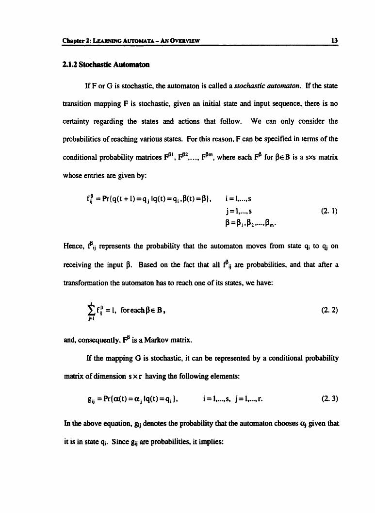
2.1.2 Stochastic Automaton

If F or G is stochastic, the automaton is called a stochastic automaton. If the state

transition mapping F is stochastic, given an initiai statc and input sequence, there is no

cenainty regarding the states and actions that follow. We cm ody consider the

probabilities of naching various states. For this reason, F can be specified in ternis of the

conditional probability matrices l?', pz,...* Pm, where each fl for BEB is a sxs mavix

whose envies are given by:

Hence, t6, represents the probability that the automaton moves from state qi to qj on

receiving the input p. Based on the fact that d l Pij are probabilities. and thrt after a

transformation the automaton has to reach one of its states, we have:

and, consequently, is a Markov matrix.

If the mapping G is stochastic, it cm be repnsented by a conditional probability

rnatrix of dimension s x r having the following elements:

gij = Pr(a(t) = a, Iq(t) = q, ), i= l , ..., S. j=l, ... ,r. (2.3)

In the above equation. gj denotes the probability that the automaton chooses q given that

it is in state qi. Since g~ are probabiiities, it implies:

Cg, =1, for each i=l . ..., S. j=l

It can be shown [22] that by a proper radefinition of states, the output lunctioa G

of any stochastic automaton can be made detemiinistic by hcnasing the number of states

in the automaton.

if the conditional probabilities f@, and g, are independent of both t and the input

sequence, the stochastic automaton is called a jked structure stochastic outomuton

(FSSA). if the transition probabilities, eij vary based on the input at each step t, the

automaton is called a variable structure stochastic automaton (VSSA).

if the transition mapping is stochastic, we can not determine precisely the state of

the automaton ai a given time. uideed, we can oniy calculate the probability with which

the automaton is in a panicular state at a given instant. These probabüities are known as

state probabilities. The state probubility vector can be defined as

X(t) = [x, (t). R? (t), ..., X , ( t)lT , w hen nr denotes the transposed mavix and

Given the input and the initial state probability vector X(O), the state probability vector at

t=l is obtained as follows:

Cbaptei 2: LEARNWG AUTOMATA - AN OVERVIEW 15

in vector focm. the equation can be wntten as:

R(1) = [FP'O) r = lt(0).

Recursively, this leads to the state probability vector at time t, as:

Wt) = [F@(~-J) r [FP('-~) )r ...[F P'O) plc(0) .

Simildy, the components of the action probability vector P(t) are defined as:

pi(t) = R(a(t) =ai ) i = 1, ... r

which can be seen to be related to Z(t) by [Il]:

This equation shows that one cm relate the state probability Il(t) to the action

probability P(t), and ihus perform the above cornputations by f i t processing IF(t) and

then computing P(t) using the output mairix.

23 The Leamhg Automa ton

The goal of an automaton is to determine the optimal action fiom a set of possible

actions. The automaton prfonns these actions in a random environment that generates a

response for each action. The following section of this chapter describes the

characteristics of the environment in which a leaming automaton operates.

--

2.2.1 The Envlraunent

The environment (see Figure 2.2) c m be defined mathematically by a triple

(A. C, B) where A=(ai , a2 . . . ., &} represents a finite input set, B=( B 1 , B2 ,. . ., pi}

(2 5 I c w) is the output set of the environment and C=(q , cz ,..., cr} a set of pendty

probabilities, when each element Ci of C corresponds to an input action ai.

Actions Environment 1 Outpuiset B A={a,, +,.-.. 9) C=(c,,~,--.,c,)

Figure 2.2: The environment

At any discrete time t (t=0,1,2,. . .) an input a(t) cm be applied to the environment

which will generate an output b(t). Usually, the output set of an environment has two

elements pi and PZ, which are considered to be O and 1 for mathematical convenience.

As a convention, an output f!(t)= 1 is considered a failure or an unfuvorcrble response or a

penalty and an output p(t)=û is considered a success or afavoruble response or a reward.

The systems that interact with an environment that generates only two output values are

considered P-models. If the output of the environment is a finite set. the systems

interacting with this type of environment are referred to as Q-models. As a M e r

generalization, when the output of the environment is a continuous d o m variable,

which assumes values in the interval [O, 11, the mode1 is referred to as an S-niodel.

The envinmments can also be classified based on their evolutionary properties. If

the penalty probabilities ci (i= 1.2,. . . J) are constant in tirne. the environment is caiied a

Cbrpter 2: L&wwG AUTOMATA - AN OVERWEW 17

stationary environment. However, if one or more penalty probabilities Ci (i= 1 1,. . . ,r) are

not constant. the envuonment is considered nonstationary.

2.2.2 Definition oî the Leamhg Automaton

A "learning" automaton is an automaton that interacts with a random

environment, having as goal to improve its behavior. It is connected to the environment

in a feedback loop, such that the input of the automaton is the output of the environment

and the output of the automaton is the input for the environment. as shown in Figure 2.3.

p ""m Environmen t

Figure 2.3: Feedback connecrion of automaton und environment.

Starting from an initial state q(O), the leaming automaton genentes the comsponding

action MO). The environment generates a response to this action, P(0). which dictates to

the automaton that based on its transition matrix F, it should change its state to q(1). This

cycle is repeated until the probabiiity of choosiag the action that bas the srnailest penalty

probability, hopefiilly, becornes as close to unity as desired.

In order to define some quantitative nomis of behavior for the learning automata,

the automata are considered to operate in a stationary randorn environment with the

penalty probabnities (cl, ~ 2 , . . ., c,). If two automata operate in such an environment. the

automaton that receives a bigger number of favorable responses from the environment is

considered better. To achieve this, the automaton has to leam to choose the "best" action.

where the "best" action is considered the action with minimum penalty probability cmin.

One basic method by which one couid learn to choose the best action is based on

the pure chance approach. if there is no a priori information regarding each action, it is

not possible to distinguish between the diffennt actions. in such case. each action is

chosen with equal probability p(t) = l/r, i=l.2,. . .,r. An automaton that uses ihis leaming

approach is called a "pure-chance automaton" and it is considered a standard for

cornparison of the behavior of the learning automata

In order to compare various leaming automata, the average penalty for r given

action probabiiity vector P(t) at time 't' is defined as:

For the "pure-chance" automaton, the average penalty is calculated to be [Il]:

An automaton is considered better than the pure-chance automaton if its average penalty

M(t) is smaller than MO at least asyrnptoticdy. as t+= . As M(t) and limM(t) are 1 3 -

random variables. one can compare E[M(t)J with W. where

Based on the cornparison with the purethance automaton. any automaton that perfomis

ktter than the pun-chance automaton is considered expedient. Mathematically, this

definition cm be expressed as foilows:

Ddlnition 2.2: A Iearning automaton is considered expedient if

lim E[M(~)] < Mo. t-b-

More strictly, the behavior of an automaton c m be characterized by the following

de finition:

Definition 23: A leaming automaton is sûid to be absolutely expedient if

where M(t) is the expected penalty probability at instant 't', and P(t) is the probability

vector.

The condition of absolute expediency imposes an inequality on the expected

penalty probability M(t) at each instant. Taking expectations again in equation (2. 15)

we obtain [Il]:

Chapter 2; LEMNWG AUTOMATA- AN OvicflVIaW U)

which shows that Ew(t)] is strictly decreasing with 't' in a i i stationary random

environments.

As stated earlier, the goal of any automatod is to leam to asymptotically choose

the best action. An automaton that achieves this goal is considered optimal.

Mathematically, the definition of optimality in the context of leaniing automata is given

as follows:

Definition 2.4: A learning automata is considered optimal if

where

Cmin-

lim p, (t) -f 1 with probability 1, t+-

(2. 17)

pb(t) is the action probability associated with the minimum penalty probability

Unfoctunately, at present. there are no optimd leming automata. ui this case.

one might aim at a sub-optimal performance, termed as eoptimaliîy [33].

Definition 2.5: Let 2, be a learning parameter. A leaming automaton is said to be E-

optimal if for every e > O and 6 > O, there exists t~ > - and 2~ > O such that

for al1 t 2 b and Â.&.

The E-optUnol defuiition Unplies that given enough time and given an intemal

parameter k (usually depending on the numkr of intemal states), the probability of

choosing the best action almost aii the tirne, can be made as close to unity as desired.

It has been shown that if an automaton is absolute expedient then, it is also

e ~ p t ~ m ~ l in al stationary random envkonments [SI.

23 Fixed Structure and Variabk S t ~ c h i r e Leamhg Automata

A variety of leiuning automata have ken proposed, beginning with Tseh ' s

pioneenng paper in 1961 [3L]. Initial leming automata designs had time invariant

transition and output hinctions, king considered "fied structure" learning automata.

Tsetlin, Krylov, and Krinsky [31] [32] presented notable examples of these automata

type. Variable Structure Stochastic Automata (VSSA) were developed later, in which the

state transition hnctions and the output hinctions were tirne dependent [Il] .

23.1 Fixed Structure Automata

23.1.1 Tsetlin Automaton

This was the fmt learning automaton pnsented in the literature 1311. It is a

detercninistic fixed structure automaton, denoted Lw2, with 2N states and 2 actions, i.e. N

states for each action. Funhennore, its s t n r t u r t can easily be extendeci to ded with

r (2 < r c -) actions. As any leaming automata, its goal is to incorporate knowledge fiom

the pst behavior of the system in its decision d e for choosing the next sequence of

actions. To achieve this, the automaton calculates the number of successes and failures

nceived for each action, and switches to the altemate action only when it receives a

suffiCient number of failuns, depending on its cumnt state. ui order to describe the

bebavior of this type of automaton. its output and state transition fùnctions will be

described below.

The output function of the automaton is simple: if the automaton is in a state

qi (1 S i S N). it chooses action ai and if it is in a state qi (N+1 I i S 2N) it chooses action

a?. Since each action has N states associated with it. N is called the memory associated

with each action and the automaton is said to have a total memory of 2N.

The state transitions are illustrated by the two graphs presented in Figure 2.4, one

for a favorable response and one for an unfavorable response. If the environment replies

with a reward (favorable response), the automaton moves deeper into the memory of the

corresponding action. if the environment replies with a pendty (unfavorable response).

the automaton moves towards the outside boundary of the memory of the corresponding

action. The deepest states in memory are refemd to as the most internal states. or the

end states.

Favorable Rcsponsc jbû

Unfavorable Rcspmse pl

Figurr 2.4: State transition graphs for the Tsetlin automaton Lm

The Tsetlin automaton can be analyzeâ using the theory of Markov chains [Il].

From this perspective. it is possible to characterize the states of the automaton as

recurrent srutes, meaning that the automaton can be in any state an infinite number of

times. For example, if the automaton is in state 1, and action 1 is being penalued N

consecutive times, and after that the automaton is rewarded N consecutive times, the

automaton will move from state 1 to state N+1. Similarly, the automaton will move from

the state N+1 to the state 1. Funhermore. the automaton is irreducible because every two

states (qi. qi) communicate [ll]. Another characteristic of this autornaton is that it is

aperiodic. since it cm loop in the states 1 and N+l an arbitrary number of times.

Any finite Markov chah that is irreducible and aperiodic is ergodic 161, and ihis

implies that the Tsetlin automaton is ergodic. This property of the Tsetlin automaton

indicates that the automaton will converge to a state probability distribution

independently of the probability distribution at the staning state.

The expected asymptotic penalty probability for the Tsetlin autornaton was shown

to be

where Ci is the penalty probability of a, ci=l-di, i=1,2 [1 I l . It bas bctn S ~ O W ~ that the

Tsetiin automaton is optimal in al1 environments whenever min (ci, q} S 0.5 11 11.

In 1964, Krinsky made an important step in the learning automata theory by

presenting another deterministic automaton, which was mptimal in al1 environments.

The next section presents this automaton in detail.

This automaton, denoted K ' w ~ , is a detenninistic automaton, and like its

predecessor, the Tsetlin automaton. is an automaton with 2N states and 2 actions. The

output hnction is identical to the output function of the Tsetlin automaton, i.e. if the

automaton is in any state qi (i=1,2 ... N) it chooses action ai. and if it is in yiy state qi

(i=N+L ,N+2...2N), it chooses action az.

The state transition function of Krinsky automaton is similar but not identical to

the state transition function of the Tsetlin automaton. When the environment replies with

a penalty, the automata exhibit the sarne behavior, i.e. they move towards the outside

margins of their cumnt action's domain. The difference lies in the way the automaia

react when the environment rewards an action. Tsetlin had his automata move exactly

one state closer or further from its intemal states for eoch reward or penaîty. The

''philosophy" behind Krinsky's automaton is to give a maximum effect for each reward.

This implies rnoving to the deepest state in the rnemory when the environment rewards an

action, and N consecutive penalties are cequired to change the action of the automaton.

in the case of a favorable response, if the automaton is in aay state qi (i=1,2 ...N), it

passes to state ql and if it is in any state qi (i=N+l,N+2.. .2N), it passes to the state q ~ + l ,

as show in Figure 2.5.

Unfavonble Response &1

Favonblc Rcsponsc

Figun 2.5: State transition graphs for the Krinsky outornaton

The expected asymptotic penalty probability for the Krinsky automaton was

calculated to:

where Ci, i=12 is the penalty probability [Il]. It can be easily shown that the Krinsky

automaton is E-optimal in al1 stationary random environments [Il].

The Tsetlin anci Knnsky automata are considend deterministic automata, since

both their output, and state transition huictions are deteministic. In order to present the

whole class of fixed stmctwe automata. the next section pcesents a leaming automaton

that is stochastic, introduced by Krylov in 1964.

Chapter 2: L-G AUTOMATA - AN OVERVIEW 26

2.3.13 Krylov Automaton

Krylov automaton ( K ~ N , ~ ) is also an automaton with W states and 2 actions, and

has the same output transition hnction as the LW2 automaton. Furthemore, Krylov's

automaton has the same state transition hinction as Lm- automaton but only when the

response of the environment is favorable. The khavior differs when the automaton is

penalized; in this situation, the behavior of the Krylov automaton is stochastic rather than

deterministic. If the automaton is penaiized. it moves towards or outwards it's intemal

states with a probability 0.5, as shown in the Figure 2.6.

Favonblt Responsc @

Unfavonblc Responsc pl

Fi- 2.6: Store transition graphs for the Kdov automason K'WJ

It is important to note that the modification made by Krylov makes the wtomaton

Goptimal in di environmeais. The expected asymptotic penalty probability is shown to

be:

Cbapter 2: LEARNLNG AUTOMATA - AN OVERVLEW 27

where h, = A , i = 1.2. As N increases, the limit becornes 1 -c i

which proves that the automaton is &-optimal (1 11.

Krylov's automaton is a fixed structure stochstic automaton (FSS A). The

concepts of the automata presented above can be extended to cases where the automata

c m perform r (2 S r < -) actions (ai, az.. . a}. The automata with many actions and the

automata with only two actions differ mainly in those states where the automaton

switches from one action to the next. A detailed description of this generalization cm be

found in [32] [Il] ,

23.2 Variable Structure Stoch astic Automata

In search for a greater flexibility for designing automata. Varshavskü and

Vorontsova [34] were the fmt to propose a class of automata that update transition

probabilities; these are called Variable Structure Stochastic Automata (VSSA). The

principal characteristic of this type of automata is that the state transition probabilities or

the action selecting probabiiities are updated with time.

For mathematical simplicity, it is assumed that each state corresponds to a distinct

action. This implies that the number of states s is equal to the number of actions

r (S = r < a) and so, the action transition mapping G becomes the identity mapping.

Varshavslrii and Vorontsova have proved that every VSSA is completely defineà by a set

of action probability updating rules, and so the state transition mapping F becomes

Cbrrptcc 2: LEABNING AUTOMATA - AN OVERWW 28

equivaient to the probability updating d e for the definition of a VSSA. The leamhg

automata operates on a probability vector P(t)=[pi(t).. . . ,p&)]' where pi(t) (i= 1,. . . .r) is

the probability that the automaton will select the action ai at the time t: pi(t)=Pr[a(t)= @].

A mathematicai description of a variable structure stochastic automaton is given below:

Definition 2.6: A variable structure stochastic automaton (VSSA) is a 4-tuple

<AB,T,P>, where A is the set of actions, B is the set of inputs of the automaton (the set

of outputs of the environment), and T:[O.l]'xB+[O, 1)' is an updating scherne such that

where P is the action probability vector. P(t)=[pi(t),pz(t), .... p&)lT. with

t

pi(t)=h[a(t)=~], i=l ,. ...r, and pi (t) = 1 for al1 't'. i=f

As in the case of FSSA, the VSSA can be analyzed using the Markov chah

theory. If the mapping T is independent of time. the probability P(t+l) is determined

completely by P(t), wbicb implies that (P(t)}rn is a discrete-homogenous Markov

process. From this perspective, diffeient mappings T can identify different types of

leaniing algorîthms. If the mapping T is chosen in such a m m e r that the Markov

process has absorbing states, the algorithm is refened to as absorbing algorithm.

Similady, non-absorbing algorithms are Markov processes with no absorbing states.

Ergodic VSS A are suitable for non-stationary environments because their behavior is

independent of their initial states. 'Chathachar and Narendra have presented different

viuieties of absorbing algorithms in [Il]. Ergodic VSSA have been proposed in [ll],

1121, [7]. The goal of a VSSA is to choose a mapping T such that the leaming algorithm

satisfies one of the performance criteria

The VSSA can be classified according to the updating probability hinctional

form. if P(t+l) is a linear function of P(t), the automaton is said to be linear, otherwise it

is considered nonlineut. Occasionally, two or more automata are combined to form a

hybrid automaton. Independent of the fom of the updating scheme, a VSSA follows

some basic leaming principles. If an action has been rewarded. the automaton

incrrases the probability for this action, decreasing the probability for al1 other actions. If

an action bas been penalized, the automaton decreases the probability for this action,

increasing the probability for ali other actions. Depending on the learning pnnciple of its

VSSA. different combinations of updating schemes c m be enumerated as:

RP (Reward-Penalty) - the probabilities are updated when the automaton is

rewarded and penalized.

RI (Rewad-Inaction) - the probabilities are updated when the automaton is

rewarded and are left unchanged when the automaton is penalized.

IP (Inaction-Penalty) - the probabilities are updated when the automaton is

pendized and are left unchanged when the automaton is rewarded.

If the mapping T is a continuous one, the automaton is considend a continuou

outumuton. The VSSA presented originaliy were continuous algorithms. In 1979,

niathachar and Oomrnen introduced discretized versions of learning VSSA [2q, which

have been later extended to yield varieties of absorbing, ergodic and estimator type of

learning automata [14] [17] [19] [18].

A general upàating scheme for a continuous VSSA operating in a stationary

environment wi th b= (O, 1 ) can be represented as follows:

If action is chosen a(t)= q , the updated probabilities are:

r

Because P(t) is a probability vector, it has to satisfy p, ( t ) = 1. which implies that j=i

when p(t) = 0

I;i pi ( t + 1) = pi (t) - h, ( m when P(t) = 1

In the above representation. the functions hj and gj have the following properties:

hj and gj are continuous hinctions (assumed for mathematical convenience [IL])

hj and gj are nonnegative hinctions,

for al1 i=1,2,. ..,r and ai i P(t) whose elements are in the open interval (0,l). As mentioned

above, if the hinctions hj and gj are linear in P(t). the automata are said to be linear.

VSSA are implemented using a Random-Number Generator (RNG). The

automaton decides on wbch action to choosc based on the action p~obability distribution

From the class of linear VSSA, the following three algorithms are relevant

because they express the three main philosophies of leaming: the linear reward-penalty

scheme (LRP), the linear reward-inaction scheme (LRù and the linear inaction-penalty

scheme (Lip) scheme. AU these schemes are explained below for leaming automata with

two actions. Their extension to multiple actions can be found in [L 11.

2.3.2.1 Linear Rewarâ-Penaity S cheme (Lw)

in a linear reward-penalty scheme, the automaton increases the probability for the

action that bas been rewarded, and decmses the probability for the action th* hûs k e n

penaiized. This method of learning gives the following updating equations:

where O d i < l and ûd2<l are the reward and penalty parameters, respectively. These

equations show that whenevcr a probability ~ ( t ) is increased. it is increased with a value

proportional with the distance to 1, namely [lopk(t)]. When a probability ~ ( t ) is

decreased, it is decreased with a value proportional with its distance to O, i-e., m(t)- The

specific case when hi=k2 it is known as the symmetric linear reward-penalty scheme

(Lw)*

The Lw scheme is ergodic. Also, it was shown that the asymptotic value of the

average penalty for the symmeeic LRp scheme is given by:

Cbapter 2: L m AUTOMATA - AN OV~RY~BW 32

2c1c* c, + c, lim E[M (t) J = - <-= t+- c, +c, 2 Mo 9

where ci and cz are the penalty probabilities. This proves that the LRP scheme is

expedient for ail initial conditions, in ail stationary environments. Since the scheme is

ergodic, it is it suitable for non-stationary environments 11 11.

23.23 LiwPr Reward-Inaction Scheme (Lu)

The basic idea of the reward-inaction scheme (LRI) is to keep the probabilities

unchanged whenever the environment replies with an unfavorable response. When a

favorable response is given, the probability of the action is increased as in the LRp

scheme. The updating equations for this scheme cm be derived from the LRp scheme by

choosing the penalty parameter A2 to be 0, and are presented as follows:

These equations indicate that tbis scheme has two absorbing States: [O,lJT and

[ l , ~ ] ~ . For example, if pi(t) becomes unity and action ai is rewarded, the probability

becomes

If the automaton is penalized at this time, then the pmbabüity remains unchaaged siace

the automaton dœs not react to penalties, which hplies that the state [L,o]~ is an

absorbing state. In an analogous marner, it can be shown that [OJf is an absorbing

state. This makes the scheme inappropriate for non-stationary environments. In any

stationary environment, the LRI Scheme has proved to be E-optimal [7].

2.3.2.3 Linear inaction-Penaity S cheme (Lw)

This scheme is based on the principle that the probabilities are updated only when

an action is king penalized and they remain unchanged when an action is rewarded.

This method of learning cm be expressed mathematically as follows:

pl (t + 1) = pi ( 0 if a( t ) =a, and P(t) = O

if a(t) = a, and P(t) = 1

if a(t) = a, and P(t) = O

It has been proved that this automaton is ergodic and expedient [7].

Al1 these schemes can be obtained fiom the equations (2.26) by giving different

values to the learning parameters Li and k2; for example, the Lw scherne cm be obtained

from these equations for hi* and the LRI scherne can be obtained for kz=O.

Lakshrnivarahan and Thathachar [ I l ] [7] studied the general behaviot of a ünear nward-

penalty scheme for diffennt parameters Ai and h2. They have shown that a scheme based

on the equations (2.26) with &(0,1] does not have any absorbing States and the nature

of convergence of {P(t)}m, is similar to that of the LRP scheme. Furthemore, they have

show that for small values of the parameter X2 relative to hi, the equation Eq. (2.26) can

generate an eoptimal scheme [Il]. This led to a LRtp scheme which is ergodic and e

optimul [IL]. This scheme was obtained by adding a small penalty term to the Lw

scheme; i.e. it can be viewed as a LRp scheme where the penalty terms are made small in

comparison with the reward t e m . The importance of this scheme is that it has a marked

ability to be used in non-stationary environments and yet bas good convergence

properties.

Another method used to improve the convergence of VSSA is CO discretize the

probability space. The next section describes this method and presents few examples of

discretized leaming automata

2.3.3 Discretized Lepnihg Automata

Pnor to introducing the concept of discretization, al1 the existing continuous

VSSA permitted action probabilities to take any value in the interval [O.LI. in their

implementation, the leaming automata use Random-Number Generator (RGN) in

determining which action to choose. In theory, an action probability cm take any vdue

between O and 1, so the RNG is required to be very accurate; however, in practice, the

probabilities are rounded-off to an accuracy depending on the architecture of the machine

that is used to implement the automaton.

In order to increase the speed of convergence of these algorithms and to minimize

the ~quinments of the RNG, the concept of discretking the probability space was

inuoduced [26] [19]. Analogous to the continuous algorithms. the discretized VSSA can

be defineci using probabiiity updating huictions, but these huictions cm take values in a

discrete f d t e space. These values divide the continuous [OJ] interval into a finite

number of continuous subintervals. The Discrete Algorithms are said to be linear if these

subintervais bave equal length, otherwise they are cailed nonlinear [%].

Like the continuous learning automata, the discretized learning automata can k

analyzed using the theory of Markov chahs, and can be divided into two categories:

ergodic or absorbing.

Following the discretkation concept, many of the continuous variable structure

stochastic automata have been discretized. Various discrete automata have ken

presented in liierature [19] 1171 [14] [26]. Al1 of the linear VSSA presented in the

previous section have corresponding discretized versions: Le. the discretized linear

reward-penalty automaton (DLRP), the discretized Linear nward-inaction automaton

(DLRd, and the discretized linear inaction-pnaity automaton (DLw) [26] 1141 1171. The

concepts of discretized automata will be presented in the following sections by

demonstrating the simil~t ies and dissimilarities between some continuous automata and

their discrete counterparts.

233.1 Discmtized Linear Rewa rd-Inaction Automaton

The àiscretized hear reward-inaction automaton @LR3 was the fmt discretized

automaton presented in the Literam [26]. In the following description of this automaton,

only two actions are considered, but the same concept appiies to a r-action (2acm)

automaton. nie basic idea of the leaming aigorithm is to makt discrete changes in the

action probabilities. The probability space [0,1] is divided into N intervals, where N is a

resolutioa parameter and is recommended to be an even integer. Since it is a reward-

inaction automaton. the updating equations do not modify the action probability vector

when the environment penalizes the automaton. When the response from the

environment is a reward, the automaton increases the probabiiity of the action that has

been chosen and decreases the probability for al1 the remaining actions.

The discretized automaton has a state associated with every possible probability

value, which determines the following set of states: Q=(qi,qz,. . . ,q~] . in every state qi, the

probability that the automaton chooses action a, is VN and the probability to choose

action a? is (1- QN). The state transition map is defined by the following equations:

q(t + 1) =cli+, . if a(t) = a, and P(t) = O

q(t+ 1) =qi-i 9 if a(t) = a, and P(t) = O

q(t+l)=qi , if a ( t) = a,or a, and P(t) = 1.

where q(t)=qi t q o or q ~ . It cm be seen that both qo and q~ are absorbing states. Based on

the probabilities associated with each state, the automaton can be described entinly by

the following action probability updating equations:

The algorithm starts with the initiai action probability vector P(0) =

nsolution ppramter N.

These equations indicate that {P(t)) khaves iike a homogenous Markov chah

with two absorbing states: [ L . o ] ~ and [O,llT. The algorithm bas been proven to be E-

optimal in dl environments [tg]. The difference between this algorithm and its

continuous version is in the rate of convergence. Oommen and Hansen have performed

simulations of the LRI and DLRl automata. and in al1 scenarios, the DLn1 automaton is

superior to the LRI automaton [19]. Their studies indicate rhat when the two automata

w e n made to learn the best action in an environment with ~ ~ - 0 . 2 and ~ ~ d . 6 , in 240

iterations the LRI automaton gave only an expected vdue of 0.99982. The DLRl scheme

gave an expected value of 0.99999 and subsequentiy the value stayed at unity. if a

stopping critenon was used, it was seen that the DLRI automaton reached 0.99 accuracy in

125 iterations and the LR1 automaton reached the same accuracy in 135 iterations.

in [14], Oornmen compared DLRi with some deterministic automata. The Table

2.1 shows a cornparison between the performance of various learning automata.

Table 2.1: Erpcrhentul comparative pe@ominnce of DLn, with other FSSA [14].

Tsetlin

pl(-) N E[pi(d

From these results, Oornmen concluded that for environments with cl > 0.5, the

DLru Mean Time For

Convergence (No. iteratbns)

DLRl is more accurate than the Tsetlin automaton. Furthemore, for a fixed N, as the

difference between the penalty probabüities is decreased, DLRi becornes mon accurate

than the T s e h and Knnsky automata. In al1 these environments, Oornmen observed that

the DLRI automaton is faster than the TseUin and Krinsky automata. It was later shown

that the DLRl scheme is E - o p t i ~ f in al1 random environments 1141.

2.33.2 Discretizeù Linear Inaction-Penalty Autamaton

Following the s a w methoci of discretization used for the reward-inaction

algorith, a discretued version of the linear inaction-penalty algorithm, denoted DLip,

was developed [14]. This algorithm bas been proved ergodic and expcdient in ai i random

environments 1141. A later ariiticialiy created absorbing version of this algorith, the

absorbing discretized linear inaction-penalty automaton, denoted ADLp, was the fmt

inaction-penalty algorithm proved to be ~ o p t i m a f [14]. Although the ADLW automaton

is &-optimal. simulation results have shown that this scheme is very accurate but slow in

convergence [14]. When the penalty probabilities are high. the automaton utilizes many

more responses of the environment than a reward-inaction automaton. Table 2.2 pnsents

some comparative results between the ADLa, the DLR1 and the ADLRp automata.

The updating d e s for the DLlp algorithm are defined in the following equations:

if a(t) = a, or a,. $(t) =O

2.3.3.3 Discretîzeà Linear Reward-Pendty Automaton

The discretized lhear reward-penalty automaton (DLRP), as i ts continuous

version, reacts to both reward and penalty responses of the environment. Similarly to the

DLRl and the DLrp automata, DLRp updates its action pcobabiîities in steps of size 1/N,

where N is a resolution paramter. The upùathg mles for this automaton are given by

the following equations:

pl (t + 1) = min l,p, (t) +- , if a(t) =al $0) =Oora(t) = a, $(t) = 1 I NI

Oommen and Chnstensen 1171 proved that the DLRp automaton is ergodic and E-

optimal in ai l random environments whenever ch, < 0.5. They also showed that by

making a stochastic modification to the transition function, the automata cm be made

ergodic iind e-optimal in ai l random environments. This modified version of the DLRp

automaton is known as the modifed discrete h e u r reward-penalty automaton, MDLRPI

and is the oniy known ergodic linear reward-penalty scherne, which is &optimal in al1

random environments. Oommen and Christensen created an absorbing version of the

DLRp automaton denoted NILRP. They showed that a discretized two-action linear

nward-penaity automaton with artificially created absorbing barriers is E-optimal in al1

random environments. It is the only symmetric E-optimal leaming automata known.

Simulation results indicated that the ADLRp scheme is extremely accurate and fast in

convergence [ 171.

Oommen and Chnstensen have also made a comparative study of the performance

and accuracy of some of the discrete hear automata [17]. The results of this study,

prcsented in Table 2.2. show that the ADLnp scheme is supenor based on counts of both

speed and accuracy.

Table 2.2: Comparative petjiormance of &, ADL,& ADLRP (c2=0.8)

These results indicate. for example, that if N=10, ci=0.6 and ~ ~ a . 8 . the DLRi

scheme converges with an expected accuracy of 0.855, and the mean time to converge

(M.T.C.) was 25.58 iterations. With the same parameters, the ADLP scherne converged

with a greater accuracy (0.93) but the rnean time to converge was much bigger, 499.1 1

iterations. The results for the ADLRp have shown that it converged with an accuracy of

0.93 and the mean time to converge was 32.45 iterations. The followhg table

summarizes the convergence characteristics of aii the VSSA, in their continuous and

discrete fonns.

T W e 2.3: Compatison between continuous a d discrete heur VSSA

continuous

discrete

continuous

discrete

discrete

con tinuous

discrete

discrete

discrete

Matkov Chain

Characterization

absorbing

absorbing

ergodic

ergodic

absorbing

ergodic

ergodic

absorbing

ergodic

Convergence Behavior

- ---

&-optimal in al1 environments

&-optimal in al1 environments

expedien t

expedient

&-optimal in dl environments

expedient in al1 stationiiry env.

&-optimal if ~ ~ ~ 4 . 5

&-optimal in al1 environments

&-optimal in dl environments

Although in this section we presented only linear schemes. it is important to note

that discrete nonlincar schemes have dso been developed [14]. A description of these is

omitted here in the interest of brevity. The next section presents a new category of

leaming algorithms, the estimator algorithms.

Cbapter 2: L-G AUTOMATA - AN O w t ~ v i ~ W 43

2.4.1 Overview

in the quest to design faster converging leaming algorithms, Thathachar and

Sastry have opened another path by introducing a new class of aigorithrns, called

estimator algorithms [28]. The main feanup of these algorithms is that they maintain

mnning estimates for the penalty pmbability of each possible action and use them in the

probability updating equations. The purpose of these estimates is to crystallize the

confidence in the rewwd capabilities of each action. In their characteristics, these

algorithms mode1 the behavior of a person that is trying to choose an action in a random

environment. In this task, the most cornmon and simple approach is to try each action a

number of times and to estimate the probability of reward for each action. The person

will most likely choose the action that has the highest reward estimate; however, uniilce

straighdorward estimation, the superior actions are dso chosen in a more likely manner

in the estimation process.

From this perspective, al1 the dgorithms presented in the pmvious sections are non-

estimator aigorithms. The main difference between the estimator algorithrns and the non-

estimaior aigorithms lies in the way the action probability vector is updated. The non-

esbator algorithxns update the pmbabiiity vector based directly on the response of the

environment. If the chosen action is rewarded, then the automaton increases the

probability of choosing this action at the next time instant. Otherwise, the action

probability of the selected action is decnased.

The estimator algonthms are characterized by the use of the estimates for each

action. The change of the probability of choosing an action is based on its current

estimated mem reward, and possibly on the feedback of the environment. The

environment determines the probability vector indirectly, thmugh the calculation of the

reward estimates for each action. Even when the chosen action is rewarded, there is a

possibility that the probability of choosing another action is increased.

For the definition of an estimator leaming automaton, a vector of reward

estimates d(t) must be introduced. Hence, the state vector Q(t) is dcfined as

Q(t) =< ~( t ) ,d ( t ) >, were &t) = [i, ( t ) ..a, (t)]' [29]

Thathachar and Sastry have shown that the estimator algorithms exhibit a superior

speed of convergence when compared with the non-estimator aigorithrns 1291. in 1989,

ûommen and LanctBt introduced discretized versions of the estimator aigorithms, and

have shown that the discretized estimator algonthms are even faster than their continuous

counterparts [ 101.

This section describes the class of continuous estimator algorithms.

Thathachar and Sastry [27] introduced the concept of estimator algorithrns by

presenting a Pursuit Algorithm that implemented a reward-penalty learning philosophy,

denoted CPRP. As its name reveals. this aigonthm is characterized by the fact that it

pursues the action that is cumntly estimated to be the optimal action. The algorithm

achieves this by increasing the probability of the current optimal action if the chosen

action was either rewarded or penalized by the environment.

The CPRP algorithm involves three steps [27]. The fmt step consists of choosing

an action a(t) based on the probability distribution P(t). Whether the rutomaton is

rewarded or penalized, the second step is to increase the component of P(t) whose reward

estimate is maximal (the cumnt optimal action), and to decrease the probability of d l

the other actions. The probability of the current optimal action is increased wiih a value

direct proportional with the distance to the unity, narnely 1-p,,,(t). AU the other

probabilities are decreased proponionally with the distance to zero, i-e. pi(t). The last

step is to update the mnning estimates for the probabiüty of king rewarded. For

caicuiating the estimates, two more vectors are ina'oduced: W(t) and Z(t), where z(t) is the number of times the 1 i action bas been chosen and Wi(t) is the number of times the

action has been rewarded. Then, the estimate vector d(t)can be calculated using the

iollowing formula:

n wi (t) di(t) =- for i=1,2,. . . ,r

Zi 0 )

Since the nst of the thesis will deal with Pursuit and estimator algorithms, we

fomally present the algorithm below.

Parameters A the speed of l e d g parameter, where O c A < 1. rn index of the maximal component of a(t), d,(t) = max{di (t)} .

i = L r

Wi(t) the number of times the ?' action has ken rewarded up to the time t. with 1SQ. Z(t) the number of times the ih action has been chosen up to the time t, with 1 % ~

Methd Initidization pi(t)=l/ï, for 1 5 i S r

Initialize d(t) by picking each action a smdl nurnber of times. Repeat

Step 1: At time t pick a(t) according to probability distribution P(t). Let Nt) = ai. Step 2: If & is the cumnt optimal action. update P(t) according to the following

equations:

Step 3: Update &t) according to the foiiowing equations:

wi (t + 1) = Wi (t) + (1 - p(t))

Zi(t+ 1) =ZJt)+ 1

Cbapter 2: L-G AUT~MATA- AN OVERWW

End R e p t END ALGORITHM CPRP

The CPRp algonthm is sirnilar in design to the LRp algorithm, in the sense that

both algorithms modify the action probability vector P(t) if the nsponse fiom the

environment is a reward or a penaity. The diffennce occurs in the way they approach the

solution. The LRp algorithm rnoves P(t) in the direction of the most recently rewarded

action or in the direction of dl the actions not penalized, whereas the CPRp algorithm

moves P(t) in the direction of the action which has the highest nward estimate.

Thathachar and Sastry proved that this algorithrn is eoptimul in every stationary

environment. Also, comparing the performance of the CPRp and LRI automata, the

authors have shown that the CPRp algorithm converges up to seven times faster than the

LRI automaton [27].

2.4.2.2 TSE Algorithm

Thathachar and Sastry in 1281 introduced a more sophisticated estimator

algorithm, which we refer to as the TSE Algorithm. Being an estimator algorithrn, it

considers the reward estimates in calculating the action probability vector. The algorithm

incnases the probabiIities for al1 the actions that have a higher estimate than the estimate

of the chosen action, and ~ C C R ~ S the probabilities of dl the actions with a smaller

estimate. The probabilities are updated based on both the reward estimates d(t) and the

action probability vector P(t), as shown below, in the detailed of this algorithm.

ALGORITHM TSE

Parameters k the speed of leming parameter, when O < A c 1. m index of the maximal cornponent of &t), dm (t) = mu{ a i (t) } .

i=t,..r

Wi(t) the number of times the rJh action has been rewarded up to the time t, with 1 L i L r Z(t) the number of times the ib action has been chosen up to the time t, with 1 5 i I r

1 if ;Li(t)>dj(t) Sij(t) an indicator function S, ( t) =

O if di(t) ~ d , ( t )

f E[- 1. II+[- 1.11 a monotonie, increasing function satisfying f(O)=û Method lniUalizaUon pi(t)=l/r, for 1 5 i S r

initiaiize d(t) by picking each action a smdl number of times. Repeat

Step 1 : At time t pick a(t) according to probability distribution P(t). Let Mt)= a. Step 2: Update P(t) according to the following equations:

Step 3: Update &t) according to the foliowing:

wi (t + 1) = Wi (t) + (1 - ~ ( t ) ) Zi ( t+l )=Zi( t )+l

End Repeat END ALGORITHM TSE

It is important to notice that P(t) depends indirectly on the response of the

environment. The feedback fiom the environment changes the values of the reward

estimate vector, which affects the values of the functions €and Sij.

The detaiied description of the algorithm indicates that if the action is

rewarded, dl the probabilities pj(t) that comspond to actions with reward estimates

higher than the reward estimate di (t) are updated using the following equation:

Since d, (t) < d (t) , the sign of the function f (d ( t ) - a, (t )) is nepative, and chus, the

probability pj(t) increases proportional to (1-pj(t)).

For al1 the actions with reward estimates smaller than ii (t) , the probabilities are

updated based on the foiiowing equation:

The sign of the function f(i , (t) - d, (t)) is positive, whkh means that the action

probability pj(t) is decreased proportionally to pj(t)-

The probability action pi(t) is incmased or decreased to ensure that the sum of al1

the action probabilities is 1. When al1 the reward estimates are higher than the reward

estimate of action a, the automaton increases ali the probabilities pj(t+l). To ensure that

the arnount that this probabilities increase does not sulpass the value of pi(t), Thathachiu

pi (t) in the updating equations. and Sastry introduced the tenn - r-1

There are two main differences between the hinuit Algorithm and the TSE

Algorithm. Fit, they differ in the method of deciding which probability actions are

increased and which are decreased. The Pursuit algorithm increases only the probability

of the action comsponding to the highest estimate, whereas the TSE Algorithm increases

the probabilities for al1 the actions with a highei nward estimate that the estimate of the

chosen action. Second, their updating cquations differ. in increasing or decreasing a

probabiiity, the TSE Aigorithm considers ais0 the distance between estimates,

incorporated in the term f (ai (t) - d,(t)), whereas the Pursuit Algorithm takes into

account only the distance between the probability at time t and the probability that it aims

for each action, O or 1.

This aigorithm bas k e n shown to be eoptimul 1291. Also, Thathachar and Sastry

presented simulation results in cornparison with the LRI scheme. They have show that

for the same level of accuracy, the TSE Algorithm often converges at least seven times

faster than the bI scheme.

The Discrete Estimator Algorithms (DEA) were introduced as an approach to

mate even faster converging leaming algorithm [9] 1101. They emerged from applying

the discretization "philosophy" to the existing estimator algorithms. In this way, the

action probabilities are aiiowed to take a finite set of values and they use the reward

estimates in their updating niles.

LanctSt and Oomrnen have defined a set of properties that every discrete

estimator algorithm must posses [9] [ 101. These properties are known as the Property of

Moderation and the Monotone Property.

Property 1: A DEA with r action and a resolution parameter N is said to posses the

properzy of moderation if the maximum magnitude by which an action probability can

decrease per iteration is bounded by VrN.

The monotone property cm be stated as below:

Property 2: Suppose there exists an index rn and a time instant b < -, such that

i, (t) > d (t) for al1 jmi and al1 t 5 to. A DEA is said to posses the Monotone Propew if

then exists an integer No such that for ail solution parameters N > No. pm(t) -+ I with

probability one as t + m.

This means that if the estimate of reward of an action a,,, remains the maximum

estimate after a certain point in t he , then a DEA bas the monotone property if it steadily

increases the probability of choosing a,,, to unity.

These properties are necessary in proving that a discretized estimator algonihm is

eoptimul. Lanctôt and Oommen have proved chat any discretized estimator algorithm

possessing both of these properties is eoptimal [9] [IO].

The discrete versions of the Pursuit Algorithm and the TSE Algorithm are

presented in the next sections of this chapter.

In 1989, Lanctôt ruid Oommen introduced a discretized version of the Pursuit

Algorithm [9] based on the nward-inaction learning "philosophy", denoted DPRi. The

differences between the discrete and continuous version of the Pursuit algonthms occur

only in the updating d e s for the action probabilities. The discrete Pursuit algorithm

malces changes to the probability vector P(t) in discrete steps, whereas the continuous

version uses a continuous function to update P(t). Being a reward-inaction algorithm, the

action probability vector P(t) is updated only when the current chosen action was

rewarded. If the c m n t action is penalized, the action probability vector P(t) remains

unchanged, which implies that the algorithm uses the estimates in updating the action

probability vector P(t) only if the environment rewards the chosen action. When the

chosen action is nwardeâ, the algorithm dec~ases the probability for al1 the actions that

do not correspond to the highest estimate, by a step A, where A=l/rN. In order to keep

the sum of the components of the vector P(t) equal to unity, the DPlu increases the

probability of the action with the highest estimate by an integral multiple of the smallest

step size A. A description of the algorithm is given below :

Parameters n index of the maximal component of &t), d m (t) = max(di (t)) .

i=l ,... r

Wi(t) the nurnber of times the f' action has been rewarded up to the tiw t, with 1 S i 5 r z(t) the number of times the ith action has been chosen up to the the t, with 1 5 i I r N resolution parameter A A = IlrN is the smallest step size Method Iniüaiizstion pi(t) = llr, for 1 S i S r

initialize d(t) by picking each action a s m d number of times. Repeat

Step 1: At time t pick a(t) according to probability distribution P(t). Let a(t) = a,. Step 2: Update P(t) according to the following equations:

if B(t) = O and pm(t) # 1

Else pj(t+I)=pj(t) for al1 1 S j Sr.

Step 3: Update the reward estimate vectord(t) (same as in the CPRP) End Repeat END ALGORITHM DPru

Oommen and LanctBt proved that this algorithm satisfies both the properties of

moderation and monotonically [18]. Also, they have shown that the algorithm is E

optimal in evecy stationary random envimnment [ 1 81.

Oommen and Lanctôt puformed simulation of the DPRI in some benchmark

environments and the results have been compared against the results of the CPRp

algorithm. The results have shown that in some difficult envinmments, the DPRi requirrs

o d y 50% of the number of iterations required for its continuous version. In a ten-action

envhmnent, the DPRI algorithm required 69% of the iterations required by the CPRI

[ l a

2.433 Dkrete TSE Algorithm

Oommen and Lanctôt also pnsented the discretized version of the TSE

Aigorithm. denoted DTSE [IO]. As the authon have said, "the design of this algorithm

is merely a compromise between the necessity of hnving the algorithm posses the

moderation and monotone properties while possessing as many qualities of the

continuous aigorithm as possible" [ 101.

Oommen and Lanctôt have justified the transformation of the TSE Algorithm into

a discretized one, by analyzing each factor that is part of the updating rules of the TSE

Aigorithm. The parameter h, representing the maximum that the continuous probability

cornponent can change. has been replaced b y the in teger O. The tenn f (i (t ) - a ( t )) was

preserved in the DTSE Aîgorithm, representing a factor of the difference between the

reward estimates. The term (t)pi (t) + si, bas been transfom~d in r-1

Sij(t) +Sji(t)- by eliminating the continuous dependency on the probability r -1

vector, as part of the discntization process.

~ h e muitant factor 8 f(di(t) -i,(t) -!-) determiner the r-1

maximum value that a probabüity WU be incnased or decreased In order to make these

changes discrete, the above factor has to be represented in terms of the number of A-

steps that pceserve also the probabilities in the interval [OJ]. To do this. two new

huictions have been introduced: Rnd(x) and Check(pi(t),pj(t)~). The Rnd() hinction

rounds up its parameter so that its value is dways an integer. The Check() fuaction

calculates the largest integer multiple of A, between 1 and x that cm be added to pi(t) and

subtracted from pj(t). and which simultaneously preserves these probabilities in the

interval [O, 11.

The algorithm modifies fint the value of the action probability that has the

highest rewvd estimate to guarantee that this value will always incnase. A description

of the algorithm is given bellow.

ALGORITHM Discrete TSE

Parameters m, Wi(t), Z,(t), SS,(t) are the same as in the TSE Algoriihm A = l/rN0, with 0 (an integer) k i n g the maximum any component cm change by. Rnd(x) rounds up x to one of (-0, -0+ 1, -0+2,. . . ,O- 1.0 ) . Ckck(pi(t),pj(t), x) r e m s the largest integer w I x such that

O S pi(t) + wA, pj(t) WA S L . Method Initialization pi(t) = llr, for 1 S i i; r

Initialize d(t) by picking eacb action a small number of times. Repeat

Step 1: At time t pick a(t) according to probability distribution P(t). Let Nt) = ai.

Step 2: Update P(t) according to the fdowing: For each action j, starhg with m Do

pi (t + 1) = P (t) - A (t), (t), change)

pi (t + 1) = pi (t) + A check(pi (t). (t), change) (2.45)

Step 3: Same as in tbe TSE Algorithm. End Reput END ALGORITHM Discrete TSE

Although the algorithm is a complicated one. Oommen and Lanctih proved that it

possesses both the modecation and the monotony properties which makes it E-optimal

E 181.

The authors have dso performed simulations in order to study the perfomance of

the discrete TSE in cornparison to its continuous version. Some of the resuits are

presented in the following table:

Table 2.4: nte number of itemtions until convergence in twosction environments for the TSE Algo nthm [IO]

I Pmbabiiity of Reward Action 1 Action 2

Mean Iterations

Continuous Discrete 1

In their simulation, the algocithrns were requhd to reach a standard rate of

accuracy of making no e m in convergence in 100 experirnents. The initiakation of

the reward estimate vector has been done in 20 iterations, which are included in the

results shown in the Table 2.4. The results have shown that the continuous TSE

algorithm was from 4 to 50% slower that the discrete TSE. For example, with di=0.8 and

d2=û.77s, the TSE aigorithm took an average of 8500 iterations to converge and the

DTSE required only 5600.

Some cornparisons were made between al1 the estimator algorithms, in two

benchmark ten-action environments.

Table 2.5: Cornparison of the discrete and continuous esrimator algorithm in benchmark ren- action environments [IO/.

EA Pursui t 1140 799

EA TSE 1310 207

1 TSE

Note: The reward probabilities used a:

EA: 0.7 0.5 03 0.2 0.4 0.5 0.4 0.3 0.5 0.2

EB: 0.1 0.45 0.84 0*76 0.2 0.4 0.6 0.7 0.5 0.3

These environments were the same ones used to compare the continuous

estimator algorithms to the LRI scheme. The estimator algorithms sampled al1 10 actions,

10 times eacb, to initialize the estimate vector. These 100 extra iterations are included in

the results presented in the Table 2.5. As the simulations of the two-action estimator

algorithm showed, the continuous version of the TSE algorithm is slower than the

discrete version; for example, in the environment refemd as EA, the DTSE takes 207

iterations to reach the end-state and the TSE takes 3 10.

These results also show that the TSE algorithm is faster than the Pursuit

Algorithm. In the same environment, the continuous Pursuit Algorithm required 1140

iterations to converge and the TSE algorithm required only 3 10. The same observation

applies to their discrete versions.

2.5 Condusions

In this chapter, different venions of known leaming automata were introduced

and presented in a comparative fashion, following their historicd development. The

main concepts were introduced at the beginning, followed by the description of the Fixed

Structure Stochastic Automata. These class of automata was exemplified by presenting

the Tsetlin's, Krinsky's and Krylov's automata. The concepts of the Variable Structure

Stochastic Automata were described afterward, and different ergodic and absorbing

versions of such automata were presented, such as LRI, LRP, LIP. Attention was focused

on the probability of converging to the optimal action in different environmenis, and on

the performance of these algonthms.

The discretization process was pnsented as a subsequent step in the evolution of

the leaming automata. By discntizing the probability space, and by approaching the

optimal solution in discrete steps instead of using continuous huictions, the convergence

of the discrete learning automata improved considerably. Discrete versions of existing

VSSA were presented, such as DLR[, DLRP, DLip. The main diffennces between these

discrete aigorithms and their continuous versions were explained.

The concepts of the Estimator Algocithms were introduced and exemplified by

pnsenting the Pursuit and the TSE algorithms, with their continuous and discrete

venions. Existing experirnental results regarding the convergence of these algorithms

were presented, and a comparative study was performed based on these results.

This chapter estabüshes the foundation for the new algorithms and results that

wiil be introduced in the following chapters.

Chapter 3: NEW PURSUIT ALGORITHMS~

3.1 Introduction

The estimator aigorithm that update the action probability vector P(t) based

solely on the running estimates consider only the long-tenn properties of the

Environment, and no consideration is given to a short-tenn perspective. In contrast. the

VSSA and the FSSA rely oniy on the short-tenn (most recent responses) properties of the

Environment for updating the probability vector P(t).

Besides these methods of incorporating the acquired knowledge into the

probability vector. another important charactenstic of the leanung automata is

represented by the philosophy of the leaming paradigm. For exampie, by giving more

importance to rewards than to penalties in the probability updating mles. the learning

automata can considerably improve their convergence properties. In the case of the linear

schemes of the VSSA, by updating the pmbability vector P(t) only if the environment

rewarded the chosen action, the linear scheme Lni becam mptimal, whereas the

' The work prrsmtcd in this chaptcr has ken published in "A C o m p N o n of Continuuus and Discre~ized Pursuit Leaming Schelllcs", authorcd by I. B. Oommen and M. Agache [la,

Chaptcr 3: NEW Rrasurr ALCORITEMS 61

symmetric linear Reward-Penalty scheme, LRP, is at most expedient. Also, by

considerably increasing the value of probability changes on reward in cornparison to

changes made on penalty, yields a resultant lineu scheme, the LR-@, which is &-optimal.

The same behavior can be observed in the case of the FSSA. The difference between the

Knnsky automaton and the Tsetlin automaton is that the Krinsky automaton gives more

importance to the rewards than to the penalties. This modification improves the

performance of the finsky automaton, making it E-optimal in ail stationary

environrnents, whereas the Tsetlin automaton is E-optimal only in the environments

where min{ci,c2) < 0.5 [3 11.

In this thesis, we argue that the automaton can mode1 the long-tenn behavior of

the Environment by maintainhg running estimates of the reward probabilities.

Additionally, we contend that the short-term perspective of the Environment is also

valuable, and we maintain that this information resides in the most recent responses thût

are obtained by the automaton. We present leaming schemes in which both the short-

rem and long-tenn perspectives of the Environment can be incorporated in the leaming

process. Specifically, the long term information is crystallized in the running reward-

probability estimates. and the use of the short term information is achieved by

considering whether the most recent response was a reward or a penalty. Thus, when

short-tenn perspectives are considered, the Reward-Inaction and the Reward-Penalty

leaniing paradigms become pertinent in the context of the estimator algorithm.

The Rusuit algorithm intmduced by Thahachar and Sastry [27] considend only

the long-term estimates in the probability updaiiag des . Lacer, ûommen and Lanctôt

Chapter 3: NEW PURSUIT A L C O i t ï ï t i ~ 62

extended the Rusuit Algorithm into the discretized world by presenting the Discretized

Punuit Algocithm. which considered both long-terni and short-tem esthates, and

implemented a reward-inaction learning philosophy [ 181. The combination of these

learning "philosophies" and paradigms, in conjunction with the continuous and discrete

computational models, le& to four versions of Punuit Lcaming Automata, listed below:

i)

ii)

iii)

iv )

Algorithm CPU: Continuous Pursuit Reward-Penalty Scheme

Paradigm: Reward-Penalty; Probability Space: Continuous

Algorithm CPW: Continuous Pursuit Reward-Inaction Scheme

Paradigm: Reward-Inaction; Probability Space: Continuous

Algorithm DPW: Discretized hrsuit Reward-Penalty Scheme

Paradigm: Reward- Penalty; Probability Space: Discretized

Algorithm DPm: Discretized Pursuit Reward-Inaction Scheme

P d g m : Reward-Inaction; Probability Space: Discretized

The CPRp and DPRi algorithms were presented in the previous chapter. This

chapter focuses on presenting the Continuous Rewardd-Inaction h u i t Algorithm and the

Discretized Reward-Penalty Pursuit Algorithm. A comparative study of the performance

of the al1 the Pursuit Algorithm is also presented.

3 3 Continuous Rew~=Iaaction Pursuit Algorithm (CPd

The continuous reward-inaction Pursuit Aigorithm npresents a continuous

version of the Discretized Pursuit Algorithm @PRù presented by Oommen and Lanct6t

[18]. It follows the same leanhg paradigm as the DPRI aigoritin, but in a continuous

probability space. If compared with the CPRP, the CPRl algorithm differs only in the

updating probabiüty rules. Being a Reward-Inaction algorithm. it updates the action

probability vector P(t) only if the current action is rewarded by the environment. When

the action is penalized. the action probability vector remains unchanged.

A formal description of the algorithm is given as follows:

ALGORITHM CPai

Parameters h m, e,, Wi(t)? &(t) : Same as in the CPRp algorithm. Methd Initiaiize pi(t) = llr, for L S 1 < r lnitialize d(t) by choosing each action a small numkr of times. Repeat

Step 1: At time t choose Nt) according to the probability distribution P(t). Let a(t) = a.

Step 2: Ua, is the action with the current highest rewûrd estimate, update P(t) as: If p(t) = O Then

P(t+l) = (1-Â) P(t) + k e,,, (3. 1) Else

P(t+ 1 )=P(t) Step 3: Update d(t) exactiy as in the CPRp Algorithm

Enà Repeat END ALGORITHM CPm

Similarly to the CPRP, the CPRl algorithm can be proven Goptimal in any

stationary environment. The proof for the E-optimaliry of the CPRi foîiows the same idea

as the other Pursuit algorithms. Fit. it can be shown that using a suficiently small

value for the leaming parameter k, al1 actions are chosen enough number of times so that

dm (t) wiii remain the maximum eiement of ihe estimate vector& t) d e r a finite time.

Mathematically, this can be expnssed as follows:

Theorem 3.1: For m y given constants 6 > O and M < -, there exist A* > O and <

such that under the CPRi aigorith, for ail XE (O, no),

Pr[Ail actions are chosen at least M times each More time t] > 1-6, for al1 t 2 t~

Proof=

Let us define the random variable Y', as the number of times the i'h action was chosen up

to time 't' in any specific realization. From the updating equation (Eq.(3.1)), at any step

't' in the algorithm. we have:

pi(t) 2 pi(t- 1 )O( 1A)

which implies that during any of the f iat 't' iterations of the algorithm

R{Q is chosen} 2 pi(0)-(1-A).)'. (3.3)

With the above clarified, reminder of the prwf is identical to the proof for the CPRp

algorithm and omitted 1271. + + * It cm be shown that if there is an action a,,,, for which the reward estimate

remains maximal after a finite number of iterations, then the mh component of the action

probability vector converges in probability to 1 (see Theorem 3.2).

Tbeorem 3.2: Suppose that there exists an index m and a time instant b c = such that

then pm(t)+l with pmbability 1 as t + -.

Chopter 3: NEW Püi~Süïï ALGORmrnts 65

Prooh

To prove this result, we shall demonstrate that the sequence of random variables

(p,,,(t))- is a submartingale. The convergence in probability WU result then fiom the

submartingale convergence theorem [ 1 11.

Based on the assumptions of the theorem. p,(t+l) can be expressed as:

pm(t+l) = pm(t) + L(1-pm(t)). if p(t)=û (i.e., with probability d,,,) (3- 4)

pm(t+ 1 ) = pm(t). if B(t)=L (i.e., with probability la,,,)

where dm is defined as km, and cm is the initial penalty probability for the action a,,,.

Then, the quantity:

A prn(t) = E[prn(t+l)- prn(t) 1 Q(t)l (3- 5 )

becomes

A pm(t) = drnA *(l-p,(t)) 2 0, for ail t 2 b, (3,6)

which implies that p,(t) is a submartingale. By the submartingde convergence theorem

[l 11, (pm(t)} converges as t + 00,

E[pdt+l)- p,(t) I Q(t)]+ O with probability 1. (3.7)

Hence, p,(t)+l with probability 1. and the theocem is proven. + * +

Finally, the Theorem 3.3 expresses the Gop~iniality convergence for the CPRi

algorithrn, and cm be easily deducted from the two previous results.

Tbeorem 3.3: For the CPRI aigonthm, in every stationary random environment, there

exists a k* c' and t&l, such that for ai i k (O, A*) and for any & (0, 1) and any EE (O, 1).

Pr[p,(t)>l-~]>1-6, forallt>b.

In order to stuày the performance of this algorithm, simulations and cornparisons

against different estimator algorithm were perfonned. The nsults are presented in the

Section 3.4.

3 3 Discretized mnl-penalty Pursuit Algorithm @PW)

A new Pursuit algonthrn, denoted DeRp, is obtained by combining the strategy of

discretizing the probability space with the Reward-Penaity learning pmdigm in the

context of a Rvsuit "philosophy". This aigorithm uses the estimates in updating the

action probability vector P(t) if the environment penalizes or rewards the chosen action.

As any discrete algorithm, the DPRp algorithm performs changes to the action probability

vector P(t) in a discrete fashion. Each component of P(t) can change with a value which

is a multiple of A, where A=llrN. r is the number of actions and N is a resolution

parameter. Fonnally. the algorithm can be expnssed as follows:

Parameters m. Wi(t), &(t), N and A : Same as in the CPRp algorithm.

Methd Initiake pi(t) = Ur, for 1 S i 5 r Mtidize &t) by choosing each action a small number of times. Repeat

Step 1: At time t choose Nt) according to probability distniution P(t). Let a(t) = a(.

Step 2: Update P(t) according to the foilowing equations: If $(t)=O and p,,,(t)# 1 Then

Cbapter 3 NEW RTRsurr ALCoRITItMs 67

Step 3: Update a(t) exactly as in the CPRp Algonthm End Repeat END ALGORITHM OPRP

Similarly to the DPRI algorithm. it is possible to show that DPRp aigorithm is E-

optimal in every stationary environment. The proof is very similar to the proof for

convergence of the DPRi and it follows the same steps. Fint, we cm prove that if the m'

action is rewarded more than any other action from time to onward then the action

probability vector P(t) for the DPRp will converge to the unit vector e,. The next theorem

captures this result:

Theorem 3.4: If then exists an index m and n time instant toc= such that dm (t) > d, (t)

for al1 j, j # m and al1 t 2 to; then there exists an integer No such that for aU resolution

parameters N > No, p,(t) -t 1 with probability 1 as t -t -.

Proott The proof for this theorem aims to show that (pm(t)}t,, is a subrnartingale

satisfyiag sup ~ [ l p, (t) l] c 0 . Then, based on the submartingale convergence theorem CM

[ 1 11 (p, (t)},,, converges, which implies

&,(t + 1) - P, ( 0 1 QW] ,, m.

where q is an integral, bounded by O and r. such that p,,,(t+l) = p,,,(t) + c, A. Thus.

~[~ , ( t + 1) -p,(t) l ~ ( t ) ] = d,c,A 2 0 , for al1 t 2 (3. 11)

which implies that p,,,(t) is a submartingale. From the submartingale convergence

theorem. this implies that dmc,A+O with prabability 1. This in implies that c,+O

w.p. 1, and consequently. max(p, (t) - A,0) + O w.p. 1. Hence p,(t) + 1 w.p. 1. jrm

The next step in proving the convergence of ihis algorithm involves showing that

using a sufficiently large value for the resolution parameter N, di actions are chosen

enough number of times so that b,(t) will remain the maximum element of the estimate

vector d(t) after a finite time.

Theorem 3.5: If for each action q, pi(0) # O. then for any given constants 6 > O and

M< -, there exists No c 00 and to c such that, under DPRP, for al1 leaming parameters

N > b a n d a l l time t>b:

R(each action chosen more than M times at time t) 2 1-5.

Pnn,I= The prwf for ihis theorem is identical with the proof for the same theorem in the

case of the DPR~ algorithm. published in [18]. + + + These two theorems lead to the conclusion that the DPRp scheme is &-optimal in

al1 stationary mdom environments.

3.4 Simulation Results

In the context of ihis study, simulations were performed in order to compare the

rates of convergence of different Pursuit Algorithm in benchmark environments. in al1

the tests performed, an aigoriihm was considered to have converged if the probability of

choosing an action exceeded a threshold T (OaSl). If the automaton converged to the

best action (Le., the one with the highest probability of being rewarded), it was

considered to have converged comctly.

Before comparïng the performance of the automata, innumerable multiple tests

were executed to detennine the "best" value of the respective learning parmeters for

each individual algorithm. The vdue was reckoned as the "kst" value if it yielded the

fstest convergence and the automaton converged to the correct action in a sequence of

NE experiments. These best parameters were then chosen as the find parameter values

used for the respective algorithms to compare their rates of convergence.

When the simulations were performed considering the same threshold T and

number of experiments, NE, as ûornmen and Lanctôt did in [18], (i.e. T=0.99 and

-79, the learning parameters obtained for the DPRi algorithm in the (0.8 0.6)

environment had a variance coefficieni' of 0.2756665 in 40 tests performed. This

variance coefficient was not considered satisfactory for comparing the performance of the

Pursuit algorithms. Subsequent simulations were performed imposing stncter

convergence requirements by increasing the threshold T, and proportionaliy, the number

' Thc variance coefficient is defined as a/M, where a is the standd deviation and M is the mean.

of experiments NE, which yielded leaming parameters with smaller variance coefficients.

For example, the leaming parameter (N) for DPRi algorithm in the (0.8 0.6) environment,

when Td.999 and NE-750, exhibits a variance coefficient of 0.0706893, which

represents a much smaller variance. Therefore, in this thesis the simulation results for

Td.999 and NE equal to 500 and 750 experiments shall be presented.

The simulations were performed in different existing benchmark environments

with two and ten actions. These environments have also been used to compare a variety

of continuous and discretized schemes, and in particular the DPRI in [18] and to compare

the performance of the CPRp against other traditional VSSA in [27]. Furthemore. to

keep conditions identical, every estimator algorithm sampled dl actions 10 times each to

initialize the estimate vector. These extra iterations are aiso included in the results

presented in the following tables. Table 3.1 and Table 3.2 contain the simulation results

for these four dgonthms is two action environments. The probability of reward for one

action was fixed at 0.8 for d l simulations and the pmbability of reward for the second

action was increased from 0.5 to 0.7~. In each case, the reported results correspond to the

results obtained using the above-described "best" parameten.

The reader will obscrw that îhere is a considembk difference betwccn the results presented hem and the results presentcd in [29]. In [29], the parameter chosen was the one which gave correct convergence in 2!5 parallel cxperimenis. However, on testing the CPRP for 1 0 experiments, it wlls observecl that it yielded only 84% accuracy. Thus, in the case of the CPRP what we seek is the largest parameter, A, which yields correct convergence in all the 750 ruid 500 qeriments respectkly. Similarly, in the case of the DPRP we seek the smaIlcst integcr parmeter, N, which yields correct convergence in al1 the 750 a d 500 crpcrinients respectively.

Cha~ter 3: NEW PURSUT ALGO~UTHMS 71

Table 3.1: Comparison of the Pursuit algorithm in two-action benchmark environments for which exact convergence was required in 750 experiments (NE= 750).

Table 3.2: Comparison of the Pursuit algorithms ln two-action benchmark environments for which exact convergence was mquired in 500 experiments (NE=500).

dl

0.8

0.8

0.8

The results of these simulations suggest that, as the difference in the reward

probabilities decreases, i.e. as the environment gets more difficult to l em, the

Dkretized Pursuit algorithms exhibit a performance superior to the Continuous

algorithms. Also. compacing the Pursuit algocithms based on the Reward-inaction

paradigm with the h e u i t algorithms based on the Reward-Penalty paradigm, one c m

notice that, in general, the Pursuit Rewilrci-Inaction algorith are up to 20% faster than

the Reward-Penalty Pursuit aigorithm. For example. if di=0.8 and d2d.6. the

discretized DPRl converges to the correct action in an average of 105.64 iterations. and

d2

0.5

0.6

0.7

dl

0.8 1

0.8

N

20

58

274

No. of

Iterat.

49.07

105.64

430.20

10.8 1 0.7 1 217 1 357.99 1 297 1 364.09 1 0.011 1 789.29 1 0.0075 1 905.36

d2

O S

0.6

N

32

89

391

No. of

Iterat.

53.74

118.24

456.13

N

17

52

h

0.214

0.046

0.009

h

0.122

0.027

0.0072

No. d

Iterat.

55.45

19832

939.63

No. d

Itemta

44.75

97

No. d

Iterak

69.69

258.60

942.88

N

26

74

No. d

Iterat,

47.9

102.17

X

0.314

0.054

No, of

Iteraî.

43.12

171.85

X

0.169

0.036

No. of

Iterat.

55.50

199.93

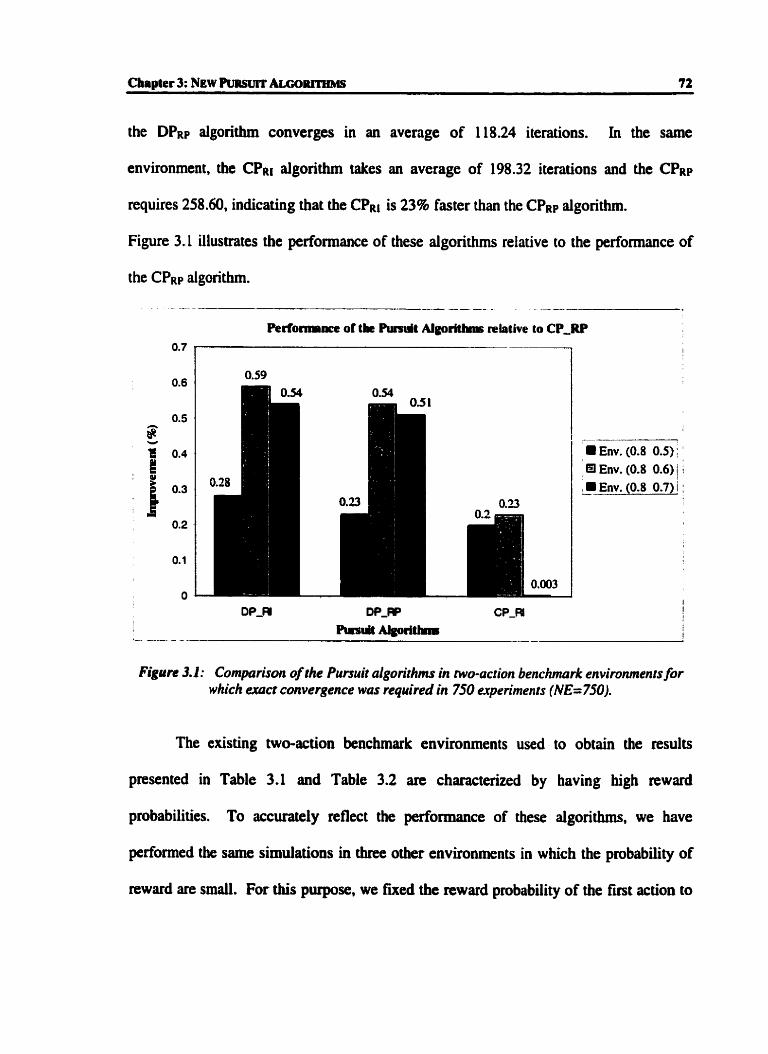
Chapter 3: NEW niRsvrr 72

the DPRp algorithm converges in an average of 118.24 iterations. In the same

environment, the CPRi algorithm takes an average of 198.32 iterations and the CPRP

requires 258.60, indicating that the CPRi is 23% faster than the CPRp aigorithm.

Figure 3.1 illustrates the performance of these algonthms relative to the performance of

the CPRp algorithm.

- -- - - ---

Pecfomnmx ofthe Rirsuit Algori- relative to CP-RP

--- Env. (0.8 0.5) :

El Env. (0.8 0.6) / I

, - i Env. (0.8 0.7) ! :

Figure 3.1: Comptarison of the Pursuit algorithm in wo-action benchmark environments for which uocr convergence war required in 750 crperiments (NE= 750).

The existing two-action benchmark environments used to obtain the results

presented in Table 3.1 and Table 3.2 are characterized by having high reward

probabilities. To accurately reflect the performance of these algorithms, we have

performed the same simulations in thm other environments in which the probability of

reward are small. For this purpose, we fixed the reward probability of the fmt action to

0.2 and we varied the reward probability of the second action fkom 0.5 to 0.3. Table 3.3

presents the results obtained in these environments.

Table 3.3: Cornparrion of the Pursuit algorithms in new two-ocrion environments for which exact convergence was required in 750 experiments (NE= 750).

The results show that also in these environments, the schemes that employed the

Reward-inaction leaming paradigm exhibit higher performance than the Rewanl-Penalty

schemes. Furthemore, the discretized schemes prove to be faster than the continuous

SC hemes.

For completeness. similar experiments were perfomed in the benchmark ten-

action environments [LS], [TOI. Table 3.4 and Table 3.5 present the results obtained in

these envuonments for 750 and 500 expenments.

b

dl

0.2

0.2

0.2

d2

OS

0.4

0.3

A,

0.349

No. d

Iteraï.

54.25

h

0.089

N

12

27

89

0.109

0.0294

No. d

Iterat.

89.25

No. d

Iterat.

51.29

108.12

403.59

I

172.14 1 0.0273

797.78 1 0.005

1

255.01

1321.1 1

N

38

100

402

No. d

Iterat.

60.16

129.69

479.69

Tuble 3.4: Compurison of the Pursuit algorithm in ten-action benchmark environments for which cmct convergence was required in 750 experimnts (NE= 750).

Note: The Reward probabilities for the actions are:

EA: 0.7 0.5 0.3 0.2 0.4 0.5 0.4 0.3 0.5 0.2

Es: 0.1 0.45 0.84 0.76 0.2 0.4 0.6 0.7 0.5 0.3

Envi

ron.

EA

Ee

Tdk 3.5: Cornpurison of the Pursuit algorithm in ten-action benchmark environrnenfs for which uocr convergence wpr required in 5W experiments (NE=500).

As in the previous two-action environments, in ten-action environments. the DPRI

algorith proved to have the best performance, converging to the correct action almost

25% faster than the DPRp aigorithm, and almost 50% faster than the CPRp algorithm. If

we malyze the behavior of these automata in the f i t environment, Eh when NE=7SO,

the average number of iterations required by the DPru to converge is 752.7, whereas the

DPRp required 1126.8, implying that the DPRi algorithm is 33% faster than the DPRp

algoritbm. In the same environment, the CPm requhs an average of 1230.3 iterations for

DPru

Envi

mn.

EA

EB

N

188

1060

No. of

Iteraî.

752.7

2693.7

DPiW

N

572

1655

DPRI

No. d

Iterat.

1 126.8

3230.3

c p ~ l

N

153

730

k

0.0097

0.002

CPRP

No. of

Iterat.

656.73

2084

DPRI

No. ol

Iterat,

1230.3

4603

A

0.003

0.00126

N

377

1230

No. of

Iterat.

2427.3

5685

No. d

Iteraî.

872.56

2511

C h

A,

0.0128

0,00225

CPRP

No. d

Iterat,

970.32

4126.58

A

0.0049

0.00128

No. of

Iterat.

1544.17

5589.54

Cbapter 3: NEW PURSUIT ALGO- 75

convergence, and the CPW requires 2427.3, which shows that the CPRl algorithm is 50%

faster than the CPRP algorithrn, and the DPRi is dmost 70% faster than the CPRP.

Based on these experimental results, we can rank the various Pursuit algonihms in

terms of their relative efficiencies - the number of iterations required to obtain the same

accuracy of convergence. The ranking is as follows:

B a t Algorithm: Discretized Pursuit Reward-Inaction (DPRi)

2ad-best Algorithm: Discretized Pursuit Reward-Penalty (DPRP)

sd-best Algorithm: Continuous Pursuit Reward-Inaction (CPRr)

4%est Algorithm: Continuous Pursuit Reward-Penalty (CPRP)

Also, the simulation results have shown that the discretized Punuit algorithms are

up to 30% fûister than their continuous counterparts. Furthemore. comparing the

Reward-Inaction Pursuit algonthms against the Reward-Penalty algorithms it cm be seen

that the Reward-Inaction algorithm are superior in the rate of convergence; they are up

to 25% faster than their Reward-Penalty counterparts.

3.5 Conclusions

This chapter extends the class of h u i t Algorithms by introducing two new

algorithms resulted from the combination of the Reward-Penalty and Reward-Inaction

leaniing paradigms in conjunction with the continuous and discrete models of

computation. The new algonthrns introduad are the Continuous Reward-Inaction

Pursuit Algorithm and the Discretized Reward-Penalty Pursuit algorithm. Furthemore,

in this chapter we argue that a leaming scheme that utilues the most recent nsponse of

the Environment permits the leaming algorithm to utilize the long-ienn and shon-rem

perspectives of the Environment.

This chapter contains a detailed description of these algorithms and the proofs of

theu convergence. Also, simulation results regarding the convergence of these

algorithms were perfonned and a quantitative cornparison between the performance of ail

the Pursuit algorithms was presented.

Overall, the Discnte Puauit Reward-Inaction aigorithm surpasses the

performance of dl the other versions of Pursuit aigonthms. Also, the Reward-Inaction

schemes are superior to their Reward-Penalty counterparts.

Chapter 4: GENERALIZATION OF TEE P~RSWT ALGORITHM~

4.1 Introduction

The main idea that characterizes the Pursuit algorithms presented in the previous

chapters is thrt they 'pursue' the best-estimated action, which is the action correspondhg

to the maximal estimate a, (t) . In any iteration, these algorithms increase only the

probabiüty of the best action, ensuring that the probability vector P(t) moves towards the

solution that has the maximal estimate at the current time. This implies that if, at any

time 't', the action that has the maximum estimate is not the action that has the minimum

penalty probability, then the automaton punues a wrong action.

In an ûttempt to minirnize this probability of pursuing a wrong action, our goal in

this chapter is to generalize the design of the Pursuit algorithm such that it pursues a set

of actions. Specificaily, these actions have higher reward estimates than the current

chosen action.

' The work presenied in ihis chapter is comprised in "Continuour md Dircretbd Generalized Purnuit Learning Schemes", authored by M. Agache and J.B. Oommen, submitted for publication at SSCI'2000 [ 11.

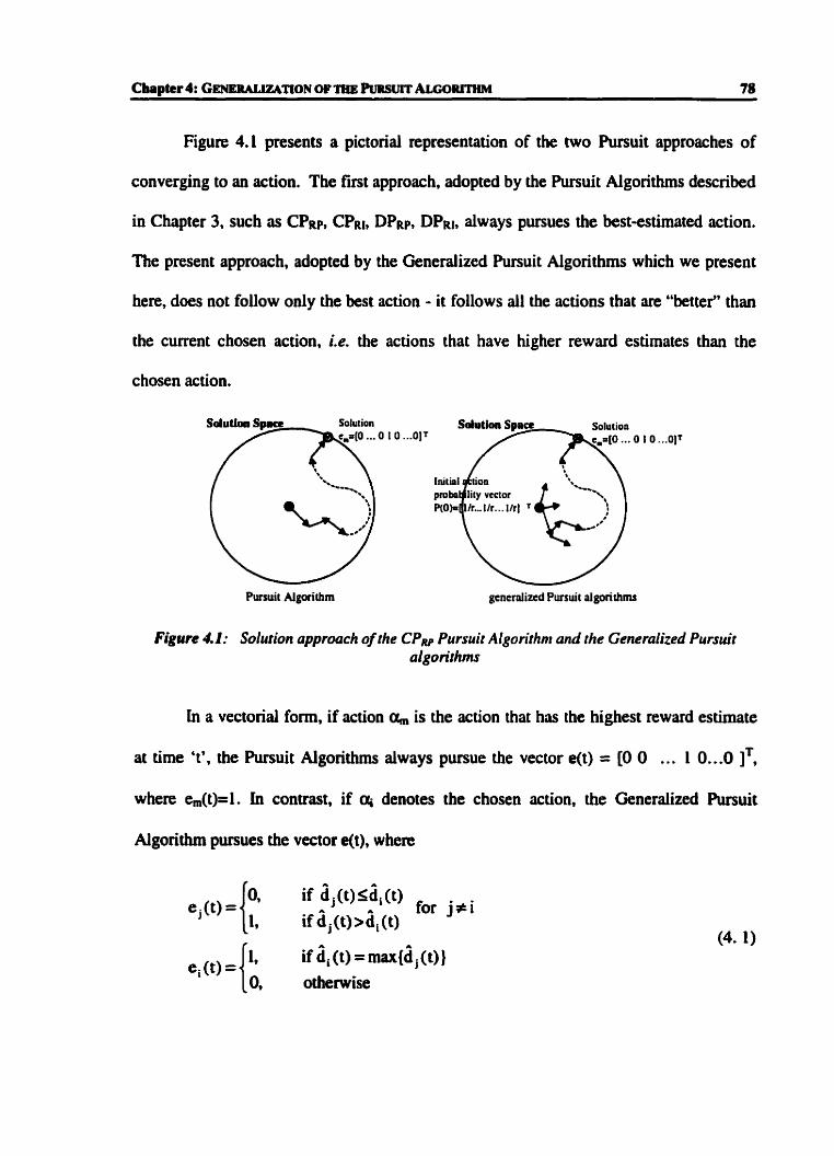
Figure 4.1 presents a pictorial representation of the two Pursuit approaches of

converging to an action. The fmt approach, adopted by the Pursuit Algorithms described

in Chapter 3, such as CPRP, CPRb DPRP, DPRl, always pursues the best-estimated action.

The present approach, adopted by the Generalized Pursuit Algorithms which we present

here, does not follow ody the best action - it follows ail the actions that are "better" than

the current chosen action, i.e. the actions that have higher reward eshates than the

chosea action.

O IO.

figure 4.1: Solution approclch of the CPRp Pursuit Algorithm and the Generalized Pursuit algorithm

In a vectoriai fom, if action a,,, is the action that has the highest reward estimate

at time 't', the Pursuit Algorithms aiways pursue the vector e(t) = [O O . . . 1 0.. .O lT,

where e,(t)=l. In contrast, if denotes the chosen action, the Generaiized Pursuit

Algorithm pursues the vector Nt), when

e j ( O = k if if é, S j(t) (t) > sir di (t) (t) for j#i

e, (t) = if ai (t) = rnax~d (t) ) otherwise

Chapter 4: G ~ R A L I W T I O N OF THE PURSUIT ALCOIUTHM 79

Since this vector e(t) represents the direction towards which the probability vector moves,

it is considered the direction vector of the Pursuit Algorithms.

This chapter presents two versions of Generalized Pursuit algorithms, followed by

a comparative study of the pedomance of these algonthms with the existing Pursuit

algorithms. The fint algorithm introduced in this chapter is the Generalized Pursuit

Algorithm. This algorithm moves the action probability vector "away" from the actions

that have smailer reward estimates, but it does not guarantee that it incnases the

probability for dl the actions with higher estimates than the chosen action.

Next, a discretized Generalized Pursuit Algorithm is presented. This aigorithm

follows the philosophy of a Generaiized Pursuit Algonthm in the sense that it increases

the action probability for dl the actions with higher reward estimates than the cumnt

chosen action.

Due to their generalized philosophy, in environments with two actions, these

algori thrns degenerate to become the exis ting Pursuit aigori thms. S pecificall y, in two

action environments, the GPA algo&.h becomes the CPw aigorithm, and the DGPA

algorithm becomes the DPRp aigorithm. For this reason, these algorithms were tested

only in benchmark ten-action environments, and the simulation results are presented in

the section 4.4 of this chapter.

The following sections present the new Generalized Pursuit Algorithms.

4.2 Genercilized Pursuit Algoritbm

The Generalued Pursuit Algorithm (GPA) presented in this section, is an example

of an algorithm that generalizes the Pursuit Algorithm introduced by Thathachar and

Sasiry in [28], referred to as the CPRp algorithm. It is a continuous estimator aigorithm.

which moves the probability vector towards a set of possible solutions in the probability

space. Each possible solution is a unit vector in which the value ' 1' corresponds to an

action that has a higher reward estimate than the chosen action.

The CPRp algorithm increases the probability for the action that has the higher

reward estimate. and decreases the action probability for al1 the other actions. as shown in

the following updating equations:

To increase the probabiiity for the best-estimated action and to dso pnserve P(t) a

probability vector, the Thathachar and Sastry's Pursuit algorithm fint decreases the

probabilities of all actions:

The remaining amount A that determines the sum of the probabilities of al1 actions to be

' 1 ' is cornputed to:

In order to hcrease the probability of the bestestimated action. the CPRp PUrSuit

algorithm adds the probabüity mass A to the probability of the best-estimated action:

In contrast to the CPRp algorithm. the newly inuoduced GPA algorithm equally

distributes the remaining amount A to al1 the actions that have higher estimates that the

chosen action. If K(t) denotes the number of actions that have higher estimates than the

chosen action rt time 't', then the updating equations for the Generaiized Punuit

Algorithm are expressed by the following equations:

pi(t + 1) = 1 - C p j ( t ) * jti

In vector form, the updating equations c m be expressed as follows:

where e(t) is the direction vector defined in (Eq 4.1).

Based on these equations, it can be seen that the GPA algorithm increases the

probability for al1 the actions with higher reward estimates than the estimate of the

chosen action, and satisfying the foiîowing inequality:

Formally, the Generaüzed Pursuit Algorithm cm be described as follows:

ALGORITHM GPA

Parameters k the leaming parameter , where O c h < 1 m index of the maximal component of d(t ). a, ( t) = max { 8, (t ) )

i = L r

Wi(t) the number of t h e s the i4 action has been rewwded up to the time t. with 1 5 i S r &(t) the number of times the P action has been chosen up to the time t, with 1 5 i I r

Method Initialization pi(t) = l/r, for 1 S i l r

Initiaiize &t) by picking each action a small number of times. Repeat

Step 1: At time t pick Mt) according to probability distribution P(t). Let a(t) = Step 2: If K(t) represents the number of actions with higher estimates than the

chosen action at time t, update P(t) according to the following equations:

Step 3:

End Repeat

j#i

Update a( t ) according to the following equations: Wi(t + 1) = Wi(t) + (1 -P(t))

Zi(t +l )=Z&t)+ 1

wj (t + 1) = wj (t) Zj(t + 1) =Z,(t) , for ai i jti 1

END ALGORITHM. GPA

As for the pnvious h u i t algorithms, the convergence of the GPA is proven in

two steps. Fit, we demonstrate that using a sufficiently small value for the leamhg

parameter k. aii actions are chosen enough number of times sucb that dm (t) wiii remain

the maximum eiement of the estimate vectord(t) dter a finite the . Formaily, this is

expressed as foiiows:

Theorem 4.1: For any given constants 6 > O and M < m. there exist A' > O and t~ < - such that under the GPA algocithm. for ail ÂE (O, kg),

Pr[Aii actions are chosen at least M times each be fore time t] > 1-6. for al1 t 2 b,

Rwl: The proof of this theonm is analogous to the proof of the corresponding result for

the TSE aigorithm. We shall consider the same randorn variable YIt as the number of

times the ih action was chosen up to time 't' in any specific realization,

From the updating equation (Eq.(4.4)),

chosen, we have:

at any step 't' in the aigocithm. if the action is

The probability of the chosen action pi(t) can either be (1 - A) pi (t - 1) . if there are other

actions with better estimates than @, or, it can be (1 - A) - pi (t - 1) + A. if the chosen

action bas the maximal reward estimate. In both these situations. the foîiowing inequality

is valid

The equations (4.9) and (4.10) show that the following inequality is valid for ai i the

actions:

Cbppttr 4: GENEMLIWTION OF THE PUR!~UIT ALGORITHM 84

which irnplies that during any of the f i t 't' iterations of the algorithm

Pr(@ is chosen) 2 ~~(o)*(l-Â)~, for any i=1,. . .,r (4. 12)

With the above clarified, the reminder of the proof is identical to the proof for the TSE

dgot-ithm and omitted (it cm be found in [28]). O * +

The second step in proving the convergence of the GPA consists of demonstrating

that if the mth action is rewarded more than any other action from time onward, then the

action probability vector converges in probability to e,. This is shown in

Theorem 4.2.

Theorem 4.2: Suppose that there exists an index m and a time instant to < - such that

then p,,,(t)+l with probability 1 as t + m.

Prook We shaU demonstrate that the sequence of random variables (p,,,(t)JW is a

submwtingaie. The convergence in probability results then from the submartingale

convergence theorem [ 1 11.

Consider

AP,,,(~) = ~ [ p , ( t + 1) - P J ~ ) IQ(OI where Q(t) is the state vector for the estimator algorithms which consists of P(t) and

d(t).

From the updating equations (4.4) and the assumptions of this theorem. pm(t+l) can have

be expressed as:

if aj ischosen j # m

This implies that for ail t 2 b, Ap,,,(t) can be calculated to be:

Apm(t) =l [^ -k rpm( t ) * ~ ~ ( t ) + [ k ( l -pm(t))l.pm = j., K(t) 1

Hence, p,(t) is a submartingale. By the submartingale convergence theorem [Il] ,

(pm(t) converges as t + œ,

E[pm(t+ 1)- pm(t) I Q(t)]+ O with pro bability 1.

Hence, p,,,(t)+l with probability 1, and the theorem is proven. + O +

Final1 y, the E-optimal convergence result can be stated as follows:

Theorem 4.3: For the GPA aigorith, in every stationary randorn environment, there

exists a h' fi and b>O, such that for ai i XE (O, h*) and for any &(O, 1) and any EE (0, 1),

~ [ ~ , ( t ) >1 -+l -6

for aii t>b. +++ The pmof for this theocem results as a logical consequence of the previous two

theorems, Theorem 4.1 and Theorem 4.2.

The simulation nsults ngarding the performance of this algorithm are presented

in the section 4.4 of this chapter. The next section presents another version of a

Generalized Pursuit aigorithm.

4 3 Discretized Generaüzed Pursuit Algorithm

The Discretized Generalized Punuit Algorithm. denoted DGPA. is another

algorithm that generalizes the concepts of the Punuit algorithm by "pursuing" al1 the

actions that have higher estimates than the current chosen action. This algorithm moves

the probability vector P(t) in discrete steps, but the steps do not have equd sizes.

At each iteration. the algorithm counts how many actions have higher estimates

than the current chosen action. If K(t) denotes this number, the DGPA algorithm

increases the probability of al1 the actions with higher estimates with the amount LVK(t),

and decreases the probabilities for al1 the other actions with the amount N(r-K(t)). where

A is a resolution step, A=l/rN with N a resolution parameter.

Vectoridly, the updating equations c m be expressed as foîlows:

where Nt) is the direction vector defined in (Eq. 4.1) and u is the unit vector uj=l,

j=12 ,..., t.

A detailed description of the algorithm is given below:

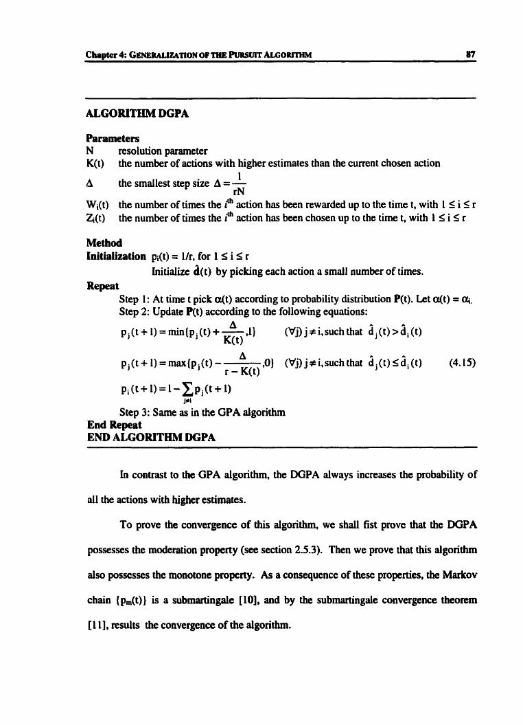
Chaptcr 4: GENL~JUWWTION OF THE W ü ï ï AM;ORtTHM 87

ALGORITHM DGPA

Parameters N resolution parameter K(t) the number of actions with higher estimates than the cumnt chosen action

1 A the smallest step size A = -

rN Wi(t) the number of times the P action has been rewarded up to the time t, with 1 S i S r z(t) the number of thes the rh action has been chosen up to the time t, with I 5 i 5 r

Metbod Initialization pi(t) = 1 Ir, for 1 S i l r

Initiaiize d(t) by picking each action a small number of times. Repeat

Step 1: At time t pick a(t) according to probability distribution P(t). Let Nt) = ai. Step 2: Update P(t) according to the following equations:

(Vj) j # i,such that 2 (t) > di (t)

p,(t + l)=rnax(pj(t)- A

,O) (b'D j F i,such that d, (t) 5 di (t) r - K(t)

jzi

Step 3: Same as in the GPA algorithm End Repe~t END ALGORITHM DGPA

In contrast to the GPA algorithm, the DGPA always increases the probability of

dl the actions with higher estimates.

To prove the convergence of thîs algorithm. we shaîi Est prove that the DGPA

possesses the moderation propecty (see section 2.5.3). Then we prove that this algorithm

also possesses the monotone property. As a consequence of these properties, the Marlrov

chah (p,(t)) is a submartingaie [10], and by the submartingale convergence theorem

[Il], results the convergence of the algorithm.

Chapter 4: GGNERALIW~ON OF THE PURSüïï AU;Oiüï"HM 88

Theorem 4.4: The DGPA possesses the moderation property.

hl: To prove this property, we shail demonstrate that the value 11rN bounds the

magnitude by which any action probability can decrease at any iteration of the algorithm:

From the updating equations (4. 15), the amount that a probability decreases is computed

to:

and the result is proven. * *+ The second step in proving the convergence of the DGPA consists of

demonstrating that the DGPA possesses the monotone property. This is shown in

Theorem 4.5.

Theorem 4.5: The DGPA possesses the monotone property.

Suppose that there exists an index m and a time instant to c - such that

&,(t) > dj(t), (VD j + m.(Wt > t,,

then there exists an integer No such that for ail N>No. p,(t)+l with probability 1 as

t+-.

Rod: The proof for this theorem aims to show that (p, (t)It, is a submartingale

satisfyiag sup ~ [ l p, (t) l] < - . Then, based on the submartingale convergence theorem UO

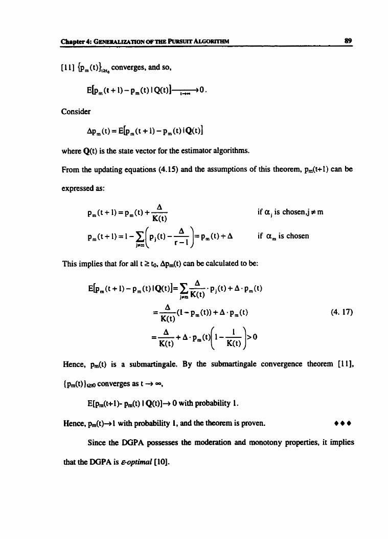
Cbapter 4: G m e w w n o ~ OF THE PURSUIT ALGOR~THM 89

&,O + l)-p,(t) IQ(~)] ,, BO-

Consider

AP&) = &,& + 1) - P&) l ~ ( t ) ]

where Q(t) is the state vector for the estimaior algorithrns.

From the updating equations (4.15) and the assumptions of this theorem, p,(t+l) cm be

expnssed as:

A p,(t+l)=p,(t)+- if a, is chosen J # m

K(t)

Pm(t + i ) = i - C pj(t)-- =pn(t )+A ( r o i ) if a, is chosen

jtm

This implies that for dl t 2 t ~ , Apm(t) can be caiculated to be:

Hence, pm(t) is a submartingale. By the submarcingale convergence theorem [Il],

{pm(t) ) rn, converges as t + -,

E[pm(t+l)- pm(t) I Q(t)]+ O with probability 1.

Hence, pm(t)+ 1 with pmbability 1, and the theorem is proven. ++* Since the DGPA possesses the moderation and wwiotoay proprties, it implies

that the DGPA is &optimal [IO].

Cbapter 4: GENERA~~WTION OF THE PURSUT ALGORITHM 90

The next section presents the simulation results for the Generalized Pusuit

algorithms introduced in this cbapter.

4.4 Simulation Results

The simulation results presented in this section have been obtained in the same

conditions as the results presented in section 3.4. First, simulations were performed in

order to determine the optimal learning parameter for each leaming aigorithm. Then,

using these learning parameters, each aigorithm was required to converge in 750

experiments and the average number of iterations was computed. For each algorithm,

100 test were performed and the number of iterations presented in this section is the

average over these experiments.

In a two-action environment. the GPA algorithm reduces in a degenente manner,

to the CPRP Pursuit algorithrn, and the MjPA reduces to DPRp aigorithm. For this reason.

simulations were performed only in ten-action benchmark environments and the results

are presented in Table 4.1. For simulation nsuits of the CPRp and DPRp algorithms, see

section 3.4.

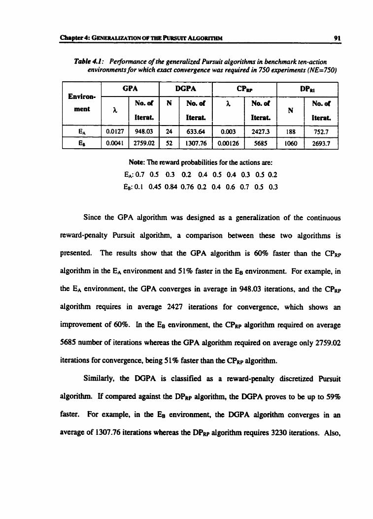
Table 4.1: Pe $ormance of the generolked Pursuit algorithrns in benchmark ten-action environments for which exacï convergence was required in 750 experiments (NE=7'iO)

Note: The reward probabilities for the actions are:

EA: 0-7 0.5 0.3 0.2 0.4 0.5 0.4 0.3 0.5 0.2

EB: 0.1 0.45 0.84 0.76 0.2 0.4 0.6 0+7 0.5 0.3

Environ-

ment

E A

EB

Since the GPA aigorithm was designed as a generalization of the continuous

reward-penalty Puauit algoriihm, a cornpuison between these two algorithms is

presented. The results show that the GPA algorithm is 60% faster than the CPRp

algorithm in the EA environment and 51% faster in the EB environment. For example, in

the Ea environment, the GPA converges in average in 948.03 iterations, and the CPRp

algorith requires in average 2427 iterations for convergence, which shows an

improvement of 60%. In the Ee environment, the CPnp algorithm required on average

5685 number of iterations whereas the GPA algorithm required on average only 2759.02

iterations for convergence, king 5 1 % faster than the C P R ~ algorithm.

Similady, the DGPA is classified as a reward-penalty discretized Pursuit

aigorithm. If compaced against the DPRp aigoritbm, the DGPA proves to be up to 59%

faster. For example, in the Es environment, the DGPA algorithm converges in an

average of 1307.76 iterations whereas the DPW algorithm quires 3230 iterations. Also,

GPA

A,

0.0127

0.0041

No.&

Iterat,

948.03

2759.02

DGPA

N

24

52

N o . d

Iteraî.

633.64

1307-76

cplv

h

0.003

0.00126

Dpni

No. of

Iterat.

2427.3

5685

N

188

1060

No. d

Iterat.

752.7

2693.7

Cbapter 4: C ~ ~ i w n o N OF= ALGORITHM 92

the DGPA algorithm proves to be the fastest Pursuit algorithm, king up to 50% faster

than the DPRi algorithm. For example, in the same environment Ee, the DGPA aigorithm

requins 1307.76 and the DPRi algorithm requires 2693 iterations for convergence.

The foiiowing figure pnsents the graphical representation of the relative

performance of these aigorithms to the CPRp algorithm in benchmark ten-action

envimnments.

----- --- -

,

; O DGPA ! B OP-RI b Q DP-RP '.-A i

'OCP I-! RI :

Figura 4.2: Perfotmunce of the Pursuit AIgorithms relative tu the CPW afgoriihm in ten-action environments for or which exact convergence was required in 750 experiments

Based on these experimental results and considering the number of iterations

required to attain the same accuracy of convergence, we can rank the six Rusuit

algorithms as follows:

Best Algorithm Discretized Generalized h u i t Algorithm (DGPA)

2"'beSt Aigorith: Discretized Pursuit Reward-Inaction @PRL)

3*-best Algorithm Generalized Rirsuit Algorithm (GPA)

4d-best Algorithm: Discretized Pursuit Reward-Penalty OPRP)

5%est Algorithm: Continuous Pursuit Reward-Inaction (CPRi)

6&-best Algorithm: Continuous Punuit Reward-Penalty (CPRP)

4.5 Conclusions

This chapter introduced another extension of the class of Pursuit estimator

algorithms by pnsenting the generalization concept of the Rusuit algorithm. The h u i t

algorithms presented in Chapters 3 "pursue" the action that has the maximal reward

estimate at any iteration. Through generalization, the generalized Pursuit aigoriihms

"punue" the actions that have higher estimates than the current chosen action,

minimizing the probability of punuing a wrong action.

Two versions of generalized Pursuit algorithms were presented in this chapter, the

Generalized Pursuit Algorithm (GPA) and the Discretized Generaiized Pursuit Algorithm

(DGPA), dong with the pcoofs for their convergence.

Simulation results were presented to characterize the performance of these

algorithms. Based on the experimental resuits, the generaîized Pursuit algoritbms prove

to be faster than Pursuit algorithms in environments with more than two actions.

Furthermore, in the same environments. the Dirretizeà Generaîized Pursuit Algorithm

proves to be the fastest converging Pursuit algorithm.

Chapter 5: GENERALIZATION OF THE TSE AL GO^

Thathachar and Sastry introduced the concept of estimator leaniing algorithms by

presenting the TSE algorithm [28]. As described in Section 2.5.2.2, the authors of this

algorithm presented its updating equations in a scalar form. in this chapter, we fmt

present a vectorid representation of the updating equations of the TSE algorithm. A

genenlization of the TSE algorithm. derived from its vectoriai fonn, is presented next,

dong with simulation results that characterize the performance of this aigorithm.

5.1 Vectodai representat ion of the TSE aigorithm

The purpose of this section is to present a vectorial representation of the TSE

aigorithm, which better outlines the underlying concepts of this algorithm.

The TSE algorithm is an estimator algorithm that moves the probability vector

P(t) towards the unit vectors associated with al1 the actions aj that have higher reward

estimates than the chosen action ai

dj(t)>di(t).

' The contributions puentcd in this chapter an cumntiy bcbg compiled in a paper ihnt wiII be submitted for pubiimtion.

Chaptcr 5: GI~EMLUATION a p ~ t i e TSE A M ; O m 95

Viewed from a scalar perspective, the updating equations can be specified as in (2.39).

where these actions are identifcd using the indicator function Sij(t). To identify the same

set of actions in vectorial fonn, a vector direcrion e(t) can be defined as foliows:

, where

iti,(t)=max(d,(t)) e , (t) =

otherwise

The actions for which e&)=L have the action probability n(t+l) increased, whereas

the actions for which ek(t)=û have the action probability ~ ( t + l ) decreased.

From the updating equations (2.39). it can be seen ihat the TSE algorithm

incnases the action probability proportional to the distance to the estimate of the chosen

action d, (t) - di (t) . To represent the same concept in a vectorial fonn, we defme a

distance matrix Fm as follows:

Chapter 5: G R ~ ~ A L ~ T I O N op THE l'SE ALGOWTHM %

..* ... . . . . m . . . . ..* Fi (t) = 1 - f ( - - r(p, (<) -a,(') ) *.. ... - f(1ii(O -J.(~)I ) 1 (5.2)

where f : [- l,l]+ 1,1] is a monotonie, increasing func tion satisfying flO)=û. It is easy to

note that computing the Fi(t) rnatrix does not increase the computational complexity of

the TSE algorithm. To define the mavix Fi(t) one has only to compute the values

f(ld,(t) -dj(t)l), for any j.1.2, .... r, as in the case of a scalar fom reprerentation.

Furthemore, as we shall see, the actual implementation does not necessarily utilize the

vector concepnialization.

To preserve P(t) as a probability vector, we introduce a weight ma& V(t) as

follows:

vij (t) = O, if j + i,

Using the above-defined matrices, the updating equations for the TSE algorithm can be

or, equivalentiy:

Cbapter 5: GENEUL~TION op THE TSE ALGORITHM 97 --

P(t + i) = (1-A*F(~) * ~ ( t ) ) * P(t) + h O F ( ~ ) V(t) -e(t) (5- 5 )

where 1 is the identity matrix of dimensions m.

The vectorial representation of the TSE algorithm6, Eq. (5.4). shows that,

concepniall y, the TSE aigorithm rnoves the action probabil i ty vector P(t) towards the

actions with higher estimates than the estimate of the current chosen action. This

movement is done proportional to the distance between the c m n t action probability

vector and the potential solutions e(t), and it involves a leaming parameter A, a factor of

the distance between the estimates, the matrix F(t), and a weight matrix V(t).

in this form, the updating equations of the TSE algorithm can easily be compared

with the following updating equation of the Continuous Reward-Penalty Pursuit

Algorithm.

P(t + 1) = P(t) + A (e, (t) - ~ ( t ) ) (5.6)

It is easy to see that the vectoriai representation of the TSE algorithm leads to various

physical interpretations of the convergence process of the TSE algorithm. Fint of dl, the

TSE algorithm "extends" the Rirsuit algorithms by punuing more than one action. i.e. it

pursues aü the actions with higher estimates. Furthemore, the equation (5.4) shows that

the TSE algorithm considers three mom factors in its updating equations: a fùnction of

the distance between the estimates, a ma& F(t), and a weight matrix V(t).

~1though wc c m represent the updating equocions of the TSE alganthm in vector form, the implementation of the algorithm can be done in a scalar fashion, as will be explained presently.

This vectoriai npresentation of the TSE algorithm sets the basis for pmiitting

various generalizations. The foiiowing section presents one such generalization of the

TSE algorithm.

5.2 Generaüzation of the TSE aigorithm

This section presents a class of algorithms that generalize the TSE algorithm by

permitting variations on the weight matrix V(t), described above. The purpose of the

weight mutrix V(t) is to ensure that the action probability vector P(t) is preserved as a

probability vector. When al1 the reward estimates are higher than the reward estimate of

the chosen action ai, the automaton incnases al1 the probabilities pj(t+l), jti. To ensure

that the amount by which these probabilities increase does not surpass the value of pi(t),

Thathachar and Sastry equally distributed the value of pi(t) to ail r-1 action with higher

pi (t) estimates. Hence, the incrernent of each probability pj(t) is multiplied with - . r -1

in this section, we present a generalized version of the TSE algorithm, denoted by

GTSE. In GTSE each increasing probability pj(t), j=l, .... K(t) is scaled with a factor

pi(t)q(t), where ~ ( t ) , j= 1,. . . ,K(t) are defined such that

and K(t) repiesents the number of actions with higher reward estimates than the chosen

action at time 't'.

Considering this, the weight matruc V(t) is defined as:

Cbapter 5: G-TION OF TSE ALGORITHM 99

The TSE algorithm becomes then a particular case of the GTSE algorithm, when y;(t)

takes the following value:

1 yj (t ) =- , for aü j= 1.. . . ,K(t).

r -1

Note that in this case the surn of ail the factors is less or equd to 1:

YI 0) + 'hW + . . + Y K ( ~ ) O ) ~ 1

Moreover, the factor y;(t) could be extended such that it represents the a prion

information about the action probabilities [14], but. at this time. this problem remains

open.

This single generalization leads us to a new learning strategy. described in detail

below.

ALGORlTHM GTSE

Parameters 5 the speed of learning parameter, where O c k c 1. m index of the maximal component of a( t ), a, (t) = max { ai (t) ) .

i d ... r

Wi(t) the number of times the ih action has been rewarded up to the time t. with 1 I i O r &(t) the nurnber of times the 1 i action has k e n chosen up to the time t, with 1 5 i d r

f E[-1 , 1 ]+l, 11 a monotonie, increasing function satisQing f(O)=û Me t h d Initirlbtio~~ pi(t)= llr, for l S i S r

Initiaiize &t) by picking each action a small number of times. Repeat

Step 1: At time t pick a(t) according to probability distribution P(t). Let Mt)= ai. Step 2: Update P(t) according to the foilowing equations:

Step 3: Update &t) according to the following:

w, (t + 1) = Wi (t) + (1 - P(t)) Zi(t + l)=Z,(t)+ 1

End R e p t END ALGORITHM GTSE

1 , for al1 j+i

As in the case of the TSE algorithrn, this generaiized version c m be proven to be

Goptimul in any stationary environment. The proof for the E-optimality of the GTSE

algorithm follows the same idea as the TSE algorithm. First, it can be shown that using a

sufficiently small value for the leaming parameter A, aîi actions are chosen enough

number of times so that a,(t) will remain the maximum element of the estimate

vectorh(t) after a finite time. Fonnally, this i s k stated and proved below.

Chapter 5: G ~ W W T I O N OF THE TSE AIGORITHM 101

Theorem 5.1: For any given constants 6 > O and M < a, there exist h' > O and < o.

such that under the GTSE algorithm. for al1 k(0, f ) ,

Pr[AU actions are chosen at least M times each before time t] 21-6. for al1 t 2 h

hf=

Let us define the d o m variable Y ' ~ as the number of times the i' action was chosen up

to tirne 't' in any specific realization. We must prove that Pr( Y'~>M)>I-~, which is

equivdent to

h[ Y', I Ml< 6. (S. 11)

The events { Y ' ~ = k} , ( Y', =j } are mutuaily exclusive for jgk. and so (5.1 1) simplifies to:

We shall prove now that if the action is chosen, then the action probability pi(t)

satis fies the following inequali ty :

pi(t)2(1-X)*pi(t-1) (5. 13)

From the updating equation (Eq.(5.10)), at any step 't' in the aigorithm if the action is

chosen, the action probability pi(t) becomes:

pi(t)=pi(t - l ) + A -

The action is chosea based on its action pmbabiiity ai tirne 't-l', and, therefore it cm

have any r e w d estimate value di (t - 1). Specificdy, the chosen action cq could eithes

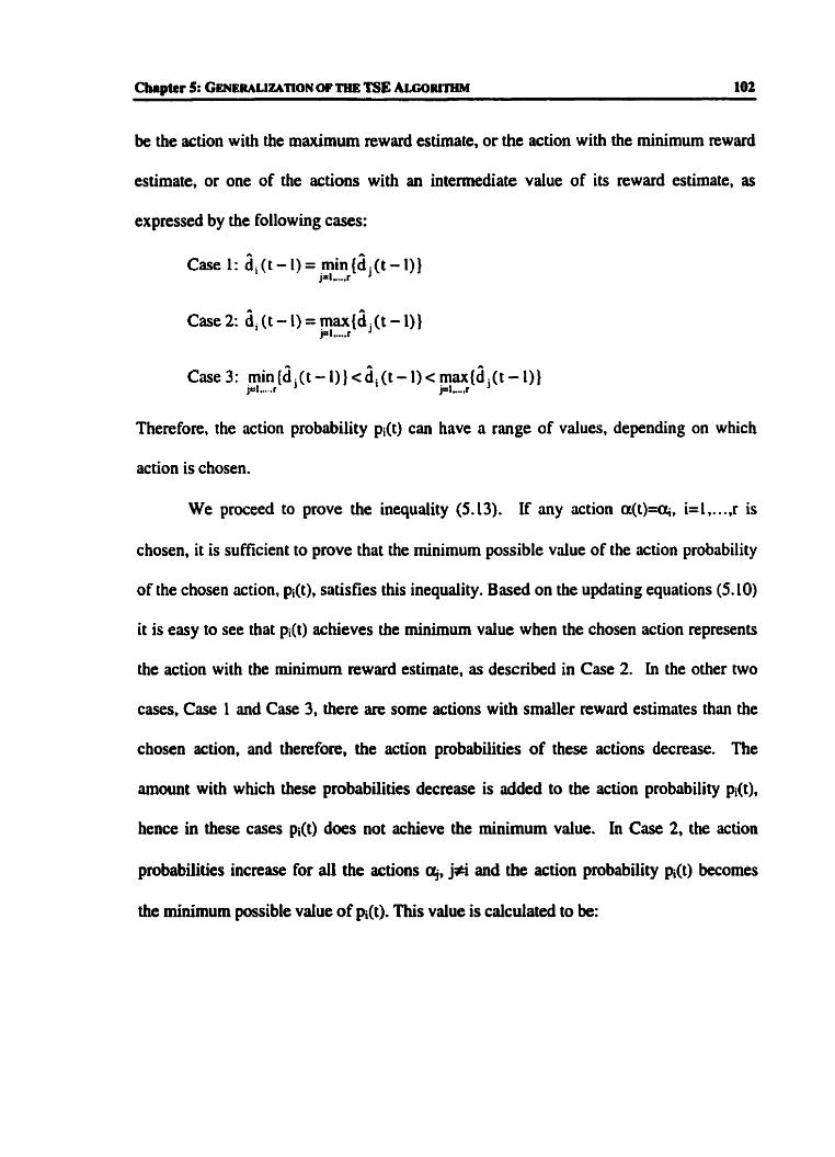
Cbapter 5: C-WTION 'ï'ïjE TSE 102

be the action with the maximum reward estimate, or the action with the minimum reward

estimate, or one of the actions with an intermediate value of its reward estimate, as

expressed by the following cases:

Case 1:

Case 2:

Case 3:

Therefore, the action probability pi(t) cm have a range of values. depenàing on which

action is chosen.

We proceed to prove the inequaüty (5.13). if any action a(t)=q. i= 1 .. . .,r is

chosen, it is sufficient to prove that the minimum possible value of the action probability

of the chosen action, pi(t), satisfies this inequality. Based on the updating equations (5.10)

it is easy to see that pi(t) achieves the minimum value when the chosen action represents

the action with the minimum reward estimate, as described in Case 2. in the other two

cases, Case 1 and Case 3, there are some actions with smaller reward estimates than the

chosen action, and therefore, the action probabilities of these actions decrease. The

arnount with which these probabilities decrease is added to the action probability pi(t),

hence in these cases pi(t) does not achieve the minimum vdue. In Case 2, the action

probabilities increase for al1 the actions aj, j#i and the action probability pi(t) becomes

the minimum possible value of pi(t). This value is calcuiated to be:

Côapter 5: CENERAWWTION OF TLlE l'SE ALGORITHM 103

Because f(x) 5 1. and pj(t) 41, this implies:

From the definition of the y;(t) factors (Eq. (5.7)) we know that the sum of these factors is

unity, which implies that

This proves that

which implies that during any of the fint 't' iterations of the aigorithm

Pr(@ is chosen) 2 pi(0)*(l-k)L, for any i=1,. ..,r

Also, at any iteration of the algorithm. Pr(@ is chosen} 51.

The reminder of the proof is identicai to the proof for the TSE aigorithm and omitted. It

can be found in [28]. + 4 *

The next step in provhg the ~ O p t i ~ f i t y of the GTSE algorithm consists of

demonstrating that if thece is an action a,,, for which the reward estimate cemains

maximal after a finite number of iterations, then the mh component of the action

Cbapter S: G E N E ~ ~ ~ Z A T I O N OF THE TSE A ~ R I T H M 104

probability vector converges in probability to 1. This result is forrnally proven in the next

theorem.

Theorern 5.2: Suppose that there exists an index m and a time instant &) c - such that

then pm(t)+ 1 with probability 1 as t + m.

To prove this resutt, we shall demonstrate that the sequence of random variables

{pm(t)}mo is a submartingaie. The convergence in probability will nsult then from the

submartingaie convergence theorem [ I l ] .

Based on the assumptions of the theorem, p,(t+l ) can take the following values:

Frorn these equations we calculate:

(5. 18) if a, ischosen

Since Ab(t+L) for ail t 2 to, implies that that pm() is a submartingale. By the

submartingale convergence theorem [ 1 11, {pm(t) ) converges as t -t 00,

Chapter 5: GENEIULIWTION OFTHE TSE A L G O R ~ ~ M 105

E[p,,,(t+l)- p,,,(t) I Q(t) ]+ O with probability 1.

Hence, pm(t)+ 1 with probability 1. and the theorem is proven. + + +

Finally. the Theorem 5.3 States the ~opt inal i ty convergence for the GTSE

aigorithm, and can be easily denved from the two previous results.

nieonm 5.3: For the GTSE algorithm, in every stationary random environment. there

exists a k* >O and @, such that for dl XE (O, A*) and for any 6~ (O, 1) and any e E (O, 1 j,

~ r [ ~ , ( t ) >LE]> 1-6

for al1 t ~ o .

This proves that this generaiized TSE algorithm is Goptimul in every stationnry

environment.

The next section presents simulation results for the GTSE algorithm

53 Simulation ResuIts

This section presents simulation results perfomed to compare the performance of

the TSE algorithm with a specific version of the Generaüzed TSE algorithm. In

simulating the GTSE algorithm, the ~ ( t ) has been assigned to be lIK(t), where K(t) is the

number of actions with higher estimates than the chosen action q(t) at tirne 't'. or 1 if the

chosen action is the one with the highest reward estimate.

The simulation envhnments that have ken considered are the same benchmark

environments as the ones for which the simulations were described in Sections 3.4 and

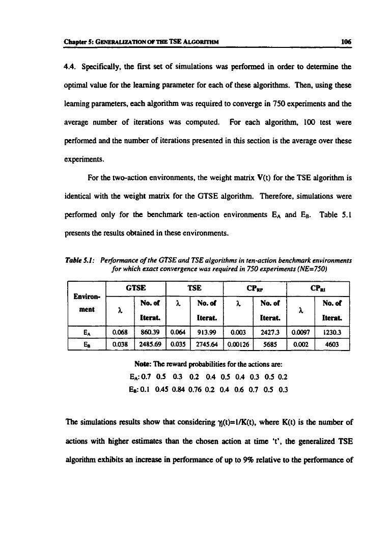
4.4. Specificdy, the first set of simulations was perfonned in order to determine the

optimal value for the leaniing parameter for each of these algorithms. Then, using these

leaming parameters, each algorithm was required to converge in 750 experiments and the

average number of iterations was computed. For each algorithm. 100 test were

performed and the number of iterations presented in this section is the average over these

experiments.

For the two-action environments. the weight matrix V(t) for the TSE dgorithm is

identical with the weight manix for the GTSE algorithm. Therefore, simulations were

performed only for the benchmark ten-action environments EA and EB. Table 5.1

presents the results obtained in these environments.

Table 5.1: Performance of the GTSE and TSE algorithms in ten-action benchmark environments for which uae t convergence was required in 750 uperimcnts (NE=7SO)

1 1 GTSE

ment L NO. or n NO. Of NO. or

h [terat. Iterat. Iterat,

Note: The reward probabilities for the actions are:

EA:0.7 0.5 0.3 0.2 0.4 05 0.4 0.3 0.5 0.2

En: 0.1 0.45 0.84 0.76 0.2 0-4 0.6 0.7 0.5 0.3

The simulations results show that considering y;(t)=l/K(t), where K(i) is the nurnber of

actions with higher estirnates than the chosen action at time 't', the generaiized TSE

algorithm exhibits an increase in performance of up to 9% relative to the performance of

Chapter 5: C m i u t t w n o ~ OF THE TSE ALGORITHM 107

the TSE algorithm. For example, in the benchmark environment EB, the TSE algorithm

required for convergence on average 2745.64 iterations. whereas the GTSE algorithm

required on average 2485.69 iterations, king 9% faster than the TSE algorithm. Also. if

compared against the class of Rusuit algoriihms, the GTSE algorithm proves to be faster

than the CPRP and CPRI algorithm. and faster than the generalized Pursuit Algorithm

GPA. For example. in the EA environment. the GTSE algorithm requires on average

860.39 iterations. whereas the CPRl requires on average 1230.3 iterations, CFRp requires

on average 2427.3 iterations for convergence. and GPA requires 948.03.

The following chart shows the improvement of the performance of the existing

continuous estimator algorithrns rrlative to the performance of the CPRp algorithm.

- - - - -

Figure 5.1: Pe@urmance of the continuous Estimator Algorithm relative ro the CPnralgorithm in ten-action environments for or which exact convergence w u required in 750 uperiments

Cbpter S: G ~ E R ~ I W T I O N OP 'R~E TSE ALGORITHM 10s

It can easily be seen that based on these experimental results, the GTSE algorithm proves

to be the fastest continuous estimator algorithm in benchmark ten-action environments.

Although the GTSE is a continuous algorithm, simulations wen executed to

compare its performance against the discretized TSE algorithm (DTSE). To obtain the

simulation results for the DTSE algorithm, we first had to determine the set of leamhg

parametea that led to the best performance of the algorithm. Unlike the other estimator

algocithms, the DTSE algorithm has two learning parametea: N, the resolution

panmeter, and 8. Therefore, we had to determine both N md 0 for which the DTSE

algorithm exhibits the best performance when nquired to converge in NE experirnents.

Rather than sewching the entire (N, 8) parameter space, we have considend just few

values of 0 (0=2, 0=10, û=100), and determined the optimal value of N for these vdues

of 0. Although the results do not span the entire parameter space, it is clear that the

results are both typical and conclusive. The best performance of the DTSE aigorithm

was obtained with 8=2. and the simulation results are presented in Table 5.2.

Chapter 5: GENEIULIWTION OF IWC TSE ALGORITHM 109

Taôle 5.2: Pe~ormance of the GTSE and DTSE algorithms in benchmark ten-action environments for which exact convergence was required in 750 erperiments (NE=750)

Note: DTSE results were obtained with 0=2.

Enviromnent

E A

Es

From these results, one can notice that the DTSE algorithrn is up to 50% faster than the

GTSE algorithm. For example, in the Ee environment. the GTSE algorithrn required on

average 2485.69 iterations to converge whereas the DTSE algorithm required on average

1 126.86 iterations.

The problem of extending the GTSE algorithrn into the discretized world remains

open,

Thathachar and Sastry introduced the TSE aigorithm [29] and presented it in a

scalar form. In this chapter, we inuoduced a vectorial representation of the TSE

dgoriihm, which led to a better conceptuai perception of the TSE algorithm. This new

vectorial form of the TSE algorithm aiso provided the background for generaliuig the

TSE algorithm by extending the weight matrix V(t).

GTSE

0.068

0.038

DTSE

No. d

Iterat.

860.39

2485.69

N

99

248

No. d

iterat.

518.18

1 126.86

Chapter 5: G E W M U Z A ~ ~ N OF nte TSE ALCORITHM 110

A class of generaüzed TSE algonthms. GTSE. has been presented in this chapter,

dong with the pcwf of their E-optimality. Simulation results have been presented for a

specifîc GTSE algorithm which considered the factors y;(t)=l/K(t), where K(t) is the

nurnber of actions with higher estimates than the chosen action at time 't'. Although the

GTSE algonthrn can be represented in vector fonn, its implementation hm k e n done in

scalar form, as presented in the detailed descnption of the algorithm.

Based on the expecimental results, we submit that the new GTSE aigorithm is

superior to the TSE aigorithm. In the ten-action benchmark environments, it exhibits an

increased performance of up to 9% when compared against the well-luiown TSE

algocithm. Furthemon, if compared against dl the existing continuous estimator

algorithrns. the GTSE algorithm proves to be the fastest one.

The generaüzation of the TSE algorithm has been presented only in a continuous

probability space. Its version in a discretized probability space remins an open problem.

We conclude this section by mentioning that the novel results of this chapter are

cumntly king compiled into a potential publication.

Chapter 6: CONCLUSIONS

6.1 Surnmary

In this thesis, we have presented a study of the reported and of some novel

Estimator Algorithms in Leaming Automata. The thesis started by presenting an

overview of the field of learning automata and of some of the most important existing

algorithms. Tsedin [31] f i t introduced the concept of a leming automaton by

designing a Fixed Structure S tochastic Automata (FSS A) traditiondl y known as the

Tsetlin Automaton. Chapter 2 presented this automaton dong with other FSSA

automata. We then introduced the farnily of Variable Structure Stochastic Automata

(VSSA), and we explained various such learning automata (e.g. LRI, LRP, Lw). The

discretkation concept was then highiighted, and the discrelized versions of the

continuous VSSA aigorithm were presented. Finally, Chapter 2 also explained the

Estimator Algorithms. by descnbing some of the existing continuous and discrete

Estimator Algorithms such as CPw, TSE, DPRi and DTSE schemes.

The thesis continued by concentrating on the study of the h u i t Estimator

Algorithms. In Chaptet 3, we presented new versions of the Pursuit algorithms that

Chapter 6: CONCLUSIONS 112

resulted from the combination of the Reward-Penalty and Reward-Inaction learning

pamdigms with the continuous and discrete models of computation. Just as in the case of

Pursuit automata, these new algorithms were shown to be eoptimal in al1 randorn

environments. Also, in this chapter we presented a performance cornparison of the newly

introduced algorithms, the CPRi and DPRP, with the already existing versions of Pursuit

algorithms, the CPRp and DPRi. Using these simulation results. we ranked these h u i t

algorithrns based on their performance as follows:

Best Algorithm: Discretized Pursuit Reward-Inaction (DPR3

2*-best Algorithm: Discntized Pursuit Reward-Penalty (DPRP)

3rd-bost Algorithm: Continuous Pursuit Reward-Inaction (CPRi)

4'h-best Algorithm: Continuous husu i t Reward-Penalty (CPRP)

In Chapter 4, we continued the study of the Puauit estimator dgonthms by

considenng two generalized versions of the CPRP Pursuit aigorithm. These new

algorithrns generaiize the Pursuit concept by attempting to linearly 'punue' not only the

action with the maximal estimate, but also dl the actions with higher reward estimates.

The new automaton, referred to as the GPA automaton, is an exarnple of a continuous

generalized Pursuit algorithm. Using these same concepts, we then presented a

discretized version. DGPA, of a genernlized Pursuit algorithm. Regarding their

convergence pmperties, we proved that these two aigorithms are optimal. As part of

the evaiuation of these new algorithrns, simulations were performed to determine their

performance. Based on the expcrimentai results obtained. we concluded that the GPA

dgodthm is the f't-converging continuous Rusuit Algoam, and that the

Chapter 6: Co~ctusto~s 113

DGPA is the fmtest àiscdc Rvsult dgorithm, and, more general, the fastest Pursuit

algorithm. From the performance perspective, we ranked the Pursuit algorithms as

follows :

Best Algorithm:

2"%est Algorithm:

3 * - k t Algorithm:

4rd-best Algorithm:

5 " - k t Algorithm:

6'-best Algorithm:

Discretized Generalized Pursuit Aigorithm (DGPA)

Discretized Pursuit Reward-Inaction (DPR [)

Generallled Pursuit Algorithm (GPA)

Discretized Pursuit Rewiud-Pend ty (DPRP)

Continuous Pursuit Reward-Inaction (CPRI)

Continuous Rirsuit Reward-Pendty (CPRP)

in Chapter 5, we concentrated on the study of the TSE estimator dgorithm,

introduced by Thaihachu and Sastry. We fiat presented a novel vectofial representation

of the updating equations of this aigorithm. This vectorial fom (Eq. (5.4)) outiines the

concepts used by the TSE aigorithm in the leaming process, and it ailows for an easy

cornparison of the TSE aigorithm with the CPRp algorithm. Furthemore, this vectorial

representation set the basis for permitting various generalizations of the TSE aigorithm.

In ihis chapter we fonnulated a generaiized TSE algorithm, nferred to as GTSE, based

on variations of the weight matrix V(t) which appears in the vectorial representation. The

GTSE dgorithm bas been presented only in the continuous probability space, its

discretization remaining an open problem. Regarding its convergence, we proved that

this algorithm is ~optimul in every stationary environment. To complete the

characterization of the newly introduced GTSE algocithm. we presented simulation

Chapter 6: Co~c~usao~s 114

results. which show that the GTSE algorithm is the fastest reported continuous

estimator dgorithm.

In conclusion, in this thesis we have introduced five new estimator algorithms:

CPRi, DPRPI GPA, DGPA and GTSE. The following graph summarizes the performance

improvement of al1 these estimator algorithm relative to the performance of the CPRp

algo ri thm.

-- -- -- - - - - - - - - -- - -- - I

0.9 r

, O DGPA DP-RI : .

jPGTSE i

;a DP-RP; i.TSE ! I

p G P A j CP-RI ; 1

1

Figure 6 I: Performance of some Estimator Algorithm relative to the CPRp algorithm in ten- action environments for which exact convergence was required in 750 crplriments

Based on the experirnental results presented in this thesis, we conclude that

among al1 the algonthms that we have analyzed, the newly introduced GPA algorithm is

the fastest continuous Rusuit dgorithm. the DOPA is the fastest converging discretized

Pursuit estimator algorithm. and, ind#d the fastest Pursuit estimator algorithm. In the

class of the continuous estimator algorithrns. the GTSE proved to be the fastest

continuous estirnator algorithm.

6 3 Future work

In this thesis. the clnss of Estimator Algorithrns has been extensively studied ûnd

various new schemes have been introduced. In spite of this. this study proved that these

dgorithms can be expanded. Furthemore. opens some new research directions.

One interesting direction that sbould be followed is to try to incorporate a priori

information in the weight matrix V(t) of the generalized TSE (GTSE) algorithm.

Additionally. since a generalization of the TSE algorithm has ken presented only in the

continuous probability space, future research coufd concentrate on generaüzing the TSE

algorithm also in the discrete space.

M. Agache, BJ. Oommen, "Continuous und Discretized Generalized Pursuit Leaming Schemes", 4' World Multiconference on Systemics, Cybemetics and Infonnatics. July 23-26. Orlando, Flonda.

K. S. Fu. "Leaming Control Systems - Review and outlook", EEE Trans. on Automatic Control, Vol. 15. pp. 210-221, April, 1970.

K. S. Fu. "Loaming Control Systems und Intelligent Control Systems: An Intersection of Artijicial Intelligence and Automatic Control ", EEE Trans. on Automatic Control, Vol. 16, pp. 70-72, 197 1.

K. S. Fu, "Pattem Recognition and Machine Learning", Plenum Press. 197 1.

K. Fukunaga, "Introduction to Statistical Pattem Recognition", Acadernic Press, 1972.

D.L. Isaacson. R.W. Madsen, "Markov Chains: Theory and Applications", New York: John Wiley&Sons, 1976.

S. Lakshrnivarahan, ''Leamhg Algoriiluns Theory and Applications", New York: S pringer-Verlag, 1 98 1.

S. Lakshmivarahan, M.A.L. Thathachar, "Absolutely Expedienr Leaming Algorithms for Stochastic Automata", IEEE Trans. Syst., Man and Cybern., SMC- 3, 1973, pp.28 1-286.

J.K. Lanctôt. "Discrete estimator algori th: A mathematical mode1 of cornputer leaming ", M.Sc. Thesis, Dept. Math. Statistics, Carleton Univ., Ottawa, Canada, 1989.

I.K. Lanctôt, B. J. Oornmen, "Discretized Estimator Leaming Automta ", EEE Trans. on Syst. Man and Cybemetics, Vol. 22, No. 6, pp. 1473-1483, November/December 1992.

K.S. Narendra, M.A.L. Thathachar, "Leamhg Automata an Introduction", Prentice-Ha& 1989.

K.S. Nanndra, M.A.L. Thathachar, "Leaming Autoniata - A survey". IEEE T m . on Syst. Man and Cybemetics, Vol. SMC-4, 1974. pp.323-334.

K.S. Narendra, E. A. Wright, L. G. Mason, "Application of Learning Autowtata tu Telephone Truflc Routing and Contruf", IEEE Trans. on Sys., Man., and Cybem., Vol. SMC-7, No. 1 1 , November 1977.

B.J. Oommen, "Absorbing and Ergodic Discretized Two-Action Learning Automata", IEEE Trans. Syst. Man Cybern., vol SMC-16. no. 4, pp.282-2996, MadApr. 1986.

B. J. Oornmen, "A Learn ing Automaton Solution to the Stochastic Minimwn- Spanning Circle Problem", IEEE Trans. Syst. Man Cybem., vol SMC-16, no. 2, pp.282-2996, JulylAugust 1986.

B.J. Oommen and M. Agache, "A Cornparison of Continuous and Discretized Pursuit Learning Schemes", IEEE. international Conference on Syst. Man. Cybem., October 12- 19, 1999, Tokyo, Japan.

B .J. Oommen and J. P. Christensen. " Epsilon-optimal discretized reward-penalty learning automata", EEE. Trans. Syst. Man. Cybem., vol. SMC-L8, pp. 45 1-458, MayIJune 1988.

B.J. Oommen and J.K. Lanctôt, "Discretized Pursuit Learning Automata ", IEEE Trans. Syst. Man. Cybem., vol. 20. No.4, pp.93 1-938, July/August 1990.

B.J. Oornmen and E.R. Hansen. "The asymptotic optimrrlity of discretized linear reward-inaction leaming automata " , IEEE. Trans. S yst. M m . Cybem., pp. 542- 545, May/June 1984.

B.J. Oornmen and G. Raghunath. "Automata Learning and intelligent Tertiary Searching for Stochastic Point Location ", IEEE. Trans. Syst. Man. Cybem. - Part B. Cybemetics, Vol. 28, No.6, pp. 947-954, December 1998.

G.I. Papadimitsiou, "A New Approach to the Design of Reinforcement Schemes for Leaming Automata: Stochasric Estimator Leaming Algotithms", IEEE Trans. on Knowledge and Data Eng.. Vol. 6, No. 4, pp. 649654, August 1994.

A. Paz, "ln troàuction to Probabil istic Automata", New York Academic Press, 1971.

J. Slagle, "Artifkial Intelligence and Heuristic Rogramrning", McGraw Hill, 1975.

R. S. Sutton, A. G. Barto, "Reinforcement Lemhg - An Introâuction'*, The MIT Press, Cambridge, Massachusetts, 1998.

R. Solomonoff, "Sotne Recent Wonk in Artijcial Intelligence", Roc. of IEEE, Vol, 54, Dec. 1966.

M.A.L. Thahachar and BJ. Oommen, "Discretized reward-inaction learning automata ", J. Cybem. Information Sci., pp.24-29, Spring 1979.

M.A.L. Thathachar and P.S. Sastry, "Pursuit Algorithnt for Learning Automata " Transcript provided by the author.

M.A.L. Thathachar and P.S. Sastry, "A class of rapidly converging algorithm for leaming automata", presented at IEEE [nt. Conf. on Cybematics and Society, Bombay, India, Jan. 1984.

M.A.L. Thathachar and P.S. Sastry, "A New Approach to the Design of Reinforcement Schemes for Leaming Automata" EEE Tms. Syst., Man. Cybem., vol SMC-15, No. 1, pp. 168- 175,JanuarylFebruary 1985.

M.A.L. Thathachar and P.S. Sastry, "Learning Optimal Discriminant Functions Through a Cooperative Game of Automuta", EEE Trans. on Systems, Man, and Cybemetics, Vol. SMC- 17, No. l,lanuary/February 1987.

M.L. Tsetlin, "On the behavior offinite autmata in random media", Automat. Telemek. (USSR), vol. 22, pp. 1345- 1354, Oct. 1961.

M.L. Tsetlin. "Autonuiton Theory and the Modeling of Biological Systents ", New York: Academic, 1973.

R. Viswanathan and K.S. Narendra, "Stochastic Automata Models with Application to Learning Systems ", EEE Trans. Syst., Man. and Cyber., SMC -3, 1973. pp. 107-1 1.

V.I. Varshavskii and LP. Vorontsova, "On the behavior of stuchasric automata with vuriable structure ", Automat. Telemek. (USSR), vol. 24, pp. 327-333, 1963.