inferring finite automata with stochastic output functions … · · 2017-08-25inferring finite...

Machine Learning, 18, 81-108 (1995)© 1995 Kluwer Academic Publishers, Boston. Manufactured in The Netherlands.

Inferring Finite Automata with Stochastic OutputFunctions and an Application to Map LearningTHOMAS DEAN [email protected] of Computer Science, Brown University, Providence, RI 02912

DANA ANGLUIN [email protected] of Computer Science, Yale University, New Haven, CT 06520

KENNETH BASYE [email protected] of Computer Science, Brown University, Providence, RI02912

SEAN ENGELSON [email protected] of Computer Science, Yale University, New Haven, CT 06520

LESLIE KAELBLING [email protected] KOKKEVISODED MARON [email protected] of Computer Science, Brown University, Providence, RI 02912

Editor: Leonard Pin

Abstract. It is often useful for a robot to construct a spatial representation of its environment from experimentsand observations, in other words, to learn a map of its environment by exploration. In addition, robots, like people,make occasional errors in perceiving the spatial features of their environments. We formulate map learning asthe problem of inferring from noisy observations the structure of a reduced deterministic finite automaton. Weassume that the automaton to be learned has a distinguishing sequence. Observation noise is modeled by treatingthe observed output at each state as a random variable, where each visit to the state is an independent trial and thecorrect output is observed with probability exceeding 1/2. We assume no errors in the state transition function.

Using this framework, we provide an exploration algorithm to learn the correct structure of such an automatonwith probability 1 — S, given as inputs 6, an upper bound m on the number of states, a distinguishing sequences, and a lower bound a > 1/2 on the probability of observing the correct output at any state. The running timeand the number of basic actions executed by the learning algorithm are bounded by a polynomial in S~l, m, \s\,and (1/2-a)-1.

We discuss the assumption that a distinguishing sequence is given, and present a method of using a weakerassumption. We also present and discuss simulation results for the algorithm learning several automata derivedfrom office environments.

Keywords: Automata inference, noisy outputs, distinguishing sequences, map learning, spatial representation

1. Introduction

In previous work (Basye & Dean, 1989, Basye et al., 1989), we have argued that robot maplearning—inferring the spatial structure of an environment relevant for navigation—can bereduced to inferring the labeled graph induced by the robot's perceptual and locomotivecapabilities. Following Kuipers and Byun (Kuipers 1978, Kuipers & Byun, 1988) and Levittet al. (1987), we assume that the robot has sensory capabilities that enable it to partitionspace into regions referred to as locally distinctive places (LDPs), and that the robot is ableto navigate between such regions reliably.

82 T. DEAN, ET AL.

The graph induced by the robot's capabilities has vertices corresponding to LDPs andedges corresponding to navigation procedures. In an office environment, the LDPs mightcorrespond to corridors and the junctions where corridors meet and the navigation proce-dures to control routines for traversing the corridors separating junctions (Dean et al., 1990).

We are interested in algorithms for learning the induced graph in cases where there isuncertainty in sensing. Uncertainty arises when the information available locally at an LDPis not sufficient to unambiguously identify it (e.g. all L-shaped junctions look pretty muchalike to a robot whose perceptual apparatus consists solely of ultrasonic range sensors).Uncertainty also arises as a consequence of errors in sensing (e.g. occasionally a T-shapedjunction might be mistaken for an L-shaped junction if one corridor of the junction istemporarily blocked or the robot is misaligned with the walls of the corridors, resulting inspurious readings from specular reflections).

In general, it is not possible for a robot to recover the complete spatial structure of theenvironment (Dudek et al., 1988) (e.g. the robot's sensors may not allow it to discriminateamong distinct structures). As a result, we will be satisfied if the robot learns the discernablestructure of its environment with high confidence. In the following sections, we will defineprecisely our use of the terms 'discernable' and 'high confidence.'

We are generally interested in the problem faced by a robot in obtaining a model ofthe dynamics of its interactions with the environment. Our motivations for studying thisproblem come from practical problems in robotics; however, the contributions of this paperare primarily theoretical. In this and related papers (Basye et al., 1989, Kaelbling et al.,1992), we extend the research on efficiently learning graphs and finite automata to handlemore realistic sources of uncertainty. In this paper, we consider the case in which movementis certain and observation is noisy and show how a robot might exploit the determinism inmovement to enable efficient learning.

We present polynomial-time algorithms for inferring an unknown deterministic finite au-tomaton with high probability given that the learner (i) can choose the actions that determinestate transitions, (ii) can observe the output associated with the state it is in with probabilitybetter than chance, and (iii) is given a distinguishing sequence. A distinguishing sequenceis a sequence of actions such that for any starting state the sequence of outputs associatedwith the states encountered in executing that sequence uniquely identifies the starting state.To determine what state it is in the robot repeatedly executes the distinguishing sequencegathering statistics and watching for patterns in the data. Given that the robot can uniquelyidentify states, learning the automaton is relatively straightforward. The rest of this paperdescribes the details.

2. Preliminaries

To formalize the problem, we represent the interaction of the robot with its environment asa deterministic finite automaton (DFA). In the DFA representation, the states correspond toLDPs, the inputs to robot actions (navigation procedures), and the outputs to the informationavailable at a given LDP. A DFA is a six tuple, M = (Q, B, Y, (, <?0,7), where

• Q is a finite nonempty set of states,

• B is a finite nonempty set of inputs or basic actions,

INFERRING AUTOMATA WITH NOISY OUTPUTS 83

• y is a finite nonempty set of outputs or percepts,

• C is the transition function, £: Q x B -» Q,

• qo is the initial state, and

• 7 is the output function, 7: Q —> Y.

Let A = B* denote the set of all finite sequences of actions, and a| denote the length ofthe sequence a € A. Let q(a) be the sequence of outputs of length |a| + 1 resulting fromexecuting the sequence a starting in q, and qa be the final state following the execution ofthe sequence a starting in q. An automaton is said to be reduced if, for all q\ ^ <j2 £ Q,there exists a € A such that qi(a) ^ qz(a). A reduced automaton is used to represent thediscernable structure of the environment; you cannot expect a robot to discern the differencebetween two states if no sequence of actions and observations serves to distinguish them.A homing sequence, h £ A, has the property that, for all q\, q? £ Q, qi (h) = q<z (h) impliesq1h = q2h. Every automaton has a homing sequence; however, the shortest homingsequence may be as long as |Q|2 (Rivest & Schapire 1989).

There are a variety of sources of supplementary knowledge that can, in some cases,simplify inference. For instance, it may help to know the number of states, \Q\, or thenumber of outputs, \Y\. It often helps to have some way of distinguishing where the robotis or where it was. A reset allows the robot to return to the initial state at any time. Theavailability of a reset provides a powerful advantage by allowing the robot to anchor all ofits observations with respect to a uniquely distinguishable state, q0. A homing sequence,h, allows the robot to distinguish the states that it ends up in immediately following theexecution of h; the sequence of observations q(h) constitutes a unique signature for stateqh. Rivest and Schapire (1989) show how to make use of a homing sequence as a substitutefor a reset. A sequence, d 6 A, is said to be a distinguishing sequence if, for all q1, q2 £ Q,q 1 ( d ) = q 2 ( d ) implies q1 = q2. (Every distinguishing sequence is a homing sequence, butnot the other way around.) A distinguishing sequence, d, allows the robot to distinguish thestates that it starts executing d in; the sequence of observations q(d) constitutes a uniquesignature for q. Not all automata have distinguishing sequences.

3. Uncertainty in observation

In this paper, we are interested in the case in which the observations made at an LDP arecorrupted by some stochastic noise process. In the remainder of this paper, we distinguishbetween the output function, 7, and the observation function, (p. We say that the outputfunction is unambigous if Vq\,qz 6 Q , j ( q 1 ) = 7(92) implies q1 = q2; otherwise, it issaid to be ambiguous. If the output function is unambiguous and ip — 7, then there is nouncertainty in observation and learning is easy.

The case in which the output function is ambiguous and ip = 7 has been studied exten-sively. The problem of inferring the smallest DFA consistent with a set of input/outputpairs is NP-complete (Angluin 1978, Gold 1978).1 Even finding a DFA polynomially closeto the smallest is intractable assuming P ^ NP (Pitt & Warmuth, 1989). Kearns and

84 T. DEAN, ET AL.

Valiant (1989) show that predicting the outputs of an unknown DFA on inputs chosenfrom an arbitrary probability distribution is as hard as computing certain apparently hardnumber-theoretic predicates. Angluin (1987), building on the work of Gold (1972), pro-vides a polynomial-time algorithm for inferring the smallest DFA given the ability to resetthe automaton to the initial state at any time and a source of counterexamples. In Angluin'smodel, at any point, the robot can hypothesize a DFA and the source of counterexampleswill indicate if it is correct and, if it is not, provide a sequence of inputs on which thehypothesized and actual DFAs generate different outputs. Rivest and Schapire show how todispense with the reset in the general case (Rivest & Schapire 1989), and how to dispensewith both the reset and the source of counterexamples in the case in which a distinguishingsequence is either provided or can be learned in polynomial time (Rivest & Schapire, 1987,Schapire, 1991).

This last result is particularly important for the task of learning maps. For many man-made and natural environments it is straightforward to determine a distinguishing sequence.In most office environments, a short, randomly chosen sequence of turns will serve todistinguish all junctions in the environment. Large, complicated mazes do not have thisproperty, but we are not practically interested in learning such environments.

The case in which (p ^ 7 is the subject of this paper. In particular, we are interested inthe case in which there is a probability distribution governing what the robot observes in astate. There are several alternatives for the sample space of the distribution governing therobot's observations.

• Each location is a single independent trial. Errors are persistent: visiting multiple timesdoesn't help.

• Each visit to a location is an independent trial. Visiting multiple times helps.

• Each location is associated with a stochastic process that depends on the time of visi-tation. Visiting at widely spaced times often helps.

• Each location/direction pair is treated distinctly. The direction from which you enter alocation matters.

In this paper, we concentrate on the case in which each visit to a location is an independenttrial. To avoid pathological situations, we assume that the robot observes the actual outputwith probability better than chance; that is,

where, in this case, ip(q) is a random variable ranging over Y. This model is a special case ofthe hidden Markov model (Levinson et al. 1983) in which state transitions are deterministicand the stochastic processes associated with the observations of states are restricted by theabove requirement. The closer a is to 1/2, the less reliable the robot's observations. In thefollowing section, we provide algorithms that allow the robot to learn the structure of itsenvironment with probability 1 — 6 for a given 0 < 6 < 1. We are interested in algorithmsthat learn the environment in a total number of steps that is polynomial in l /<5 ,1/ (a —1/2),|Q|, \B\, and \Y\. We assume that the robot is given a.


We do not consider the case in which the robot remains in the same state by repeatingthe empty sequence of actions and observes the output sufficiently often to get a good ideaof the correct output. Our rationale for not considering this case is that the independenceassumption regarding different observations of the same state is not even approximatelysatisfied if the robot does not take any overt action between observations, whereas if thereare overt actions between observations, the observations are more likely to be independent.

Note that it is often possible to determine whether your observations are seriously cor-rupted (e.g. you notice fog, rain or some other obscuring process). This ability effectivelyimproves the accuracy of your observations.

4. Learning algorithms

In the following, we present a high-probability, polynomial-time procedure, LOCALIZE,for localizing the robot (directing the robot to a state that it can distinguish from all otherstates), and then show how this procedure can be used to learn environments in which therobot is given a distinguishing sequence.2 Finally, we discuss how LOCALIZE might beused to learn a distinguishing sequence in certain cases in which a distinguishing sequenceis guaranteed to exist. We do not assume a reset. We do, however, assume that the transitiongraph is strongly connected (that is, every state is reachable by some sequence of actionsfrom every other state), thereby avoiding the possibility that the robot can become trappedin some strongly connected component from which it can never escape.

4.1. The localization procedure

The procedure LOCALIZE works by exploiting the fact that movement is deterministic. Thebasic idea is to execute repeatedly a fixed sequence of actions until the robot is certain to be"going in circles" repeating a fixed sequence of locations visited, corresponding to a cyclicwalk in the underlying deterministic automaton. If we knew the period of repetition of thesequence of locations, we could keep separate statistics on the outputs observed at eachlocation. These statistics could then be used to deduce (with high probability) the correctoutputs at those locations, and hence to localize the robot by supplying a signature for thestate the robot is in.

The problem then is to figure out the period of repetition of the walk with high probability.We keep statistics for the alternative hypotheses for the period of the cycle, which are thenanalyzed to determine with high probability the true period of the cycle.

This analysis is complicated by the fact that distinct states may be mistakenly conflatedif only local information is used. This can be seen in the simple example of a machinewith six states, one input symbol, a, and three output symbols, b, c, and d. Inputs causetransitions from state i to state i + 1 mod 6. Output probabilities are as follows:

86 T. DEAN, ET AL.

State

012345

6

.5100

.5100

c

.4901010

d

010

.4901

We can now gather output statistics for this machine while repeating the distinguishingsequence, and test different hypotheses as to the walk's period. For the hypothesis of periodtwo, we expect to see the output with frequencies:

States

{0,2,4}{1,3,5}

b

.17

.17

c

.830

d

0.83

This table looks quite plausible, so we could be led to the (erroneous) conclusion thatthe automaton has two states, with outputs c and d. This sort of 'state conflation' can beavoided by combining information gotten by considering different period hypotheses, aswe shall see below.

Recall that the Markov assumption implies a stationary probability distribution over theoutputs at each state. If the states are numbered from 1 to n and the outputs are cr, forj = 1,2,..., k, let ai,j denote the probability of observing symbol a^ given that the robotis in state i.

We assume an upper bound m on the number of states of the automaton. Let s =b1b2 ... b|8| be a sequence of one or more basic actions; we assume that s is a distinguishingsequence for the underlying automaton. Let qi be the state reached after executing thesequence of actions sm+i that is, m repetitions of s followed by i repetitions of s. The firstm repetitions ensure that the robot is in the cyclic walk. The sequence of states q0, q1, q2,...is periodic; let p denote the least period of the cycle. Note that p < m. Our main goal is todetermine (with high probability) the value of p.

For each I = 0 , . . . , |s| — 1, we also consider the sequence of states q\ reached afterexecuting the sequence of actions sm+ib1b2 • • • bf. That is, q\ is the state reached fromqi by executing the first t basic actions from the sequence s. For each £, the sequence9o > l{' <?21 • • • is also periodic of period p.

For each (., consider the sequence of (correct) outputs from the states q\:

The output sequence


is also periodic, of some least period pe dividing p. Since we are not assuming the outputsare unambiguous, pg may be smaller than p. We can show, however, that p will be the leastcommon multiple (LCM) of all the pt's.

It is clear that p is a multiple of each pe, so suppose instead that the LCM p" of all the pisis a proper divisor of p. This implies that as we traverse the cycle of p distinct states,

the output sequences qi(s) must repeat with period p" < p, which implies that two dis-tinct states have the same sequence of outputs, contradicting the assumption that s is adistinguishing sequence.

Thus, it would suffice if we could determine each of the values pf, and take their LCM.In fact, what we will be able to do is to determine (with high probability) values re suchthat pe divides re and re divides p - this also will be sufficient. To avoid the superscripts,we describe the procedure for the sequence q0, q1, q2, • • •', it is analogous for the others.

Consider any candidate period TT < m, and let g be the greatest common divisor of p andTT (GCD(p, TT)). For each 0 < i < •K - 1, consider the sequence of states visited every TTrepetitions of s, starting with m + i repetitions of s. This will be the sequence of states

Since qi is periodic of period p, this sequence visits each state of the set {qi+kg : k =0,1, . . . ,p/g — 1} in some order, and then continues to repeat this cycle of p/g states.

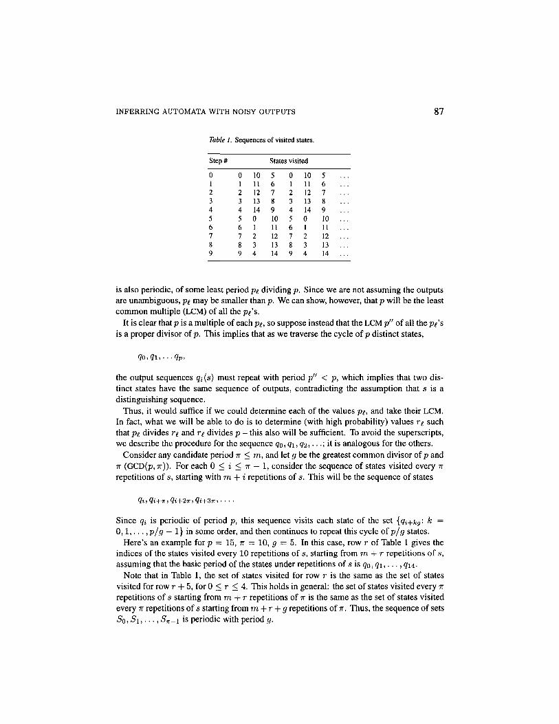
Here's an example for p = 15, ?r = 10, g — 5. In this case, row r of Table 1 gives theindices of the states visited every 10 repetitions of s, starting from m + r repetitions of s,assuming that the basic period of the states under repetitions of s is q0, q1, ... q14.

Note that in Table 1, the set of states visited for row r is the same as the set of statesvisited for row r + 5, for 0 < r < 4. This holds in general: the set of states visited every •nrepetitions of s starting from m + r repetitions of TT is the same as the set of states visitedevery TT repetitions of s starting from m + r + g repetitions of TT. Thus, the sequence of sets5o, Si , . . . , STT-I is periodic with period g.

Table 1. Sequences of visited states.

Step#

0123456789

0123456789

101112131401234

States visited

567891011121314

0123456189

101112131401234

56789 ...10 ...11 ...12 ...13 ...14 ...

88 T. DEAN, ET AL.

In the special case TT = p, row r will consist exclusively of visits to state qr. In the specialcase g — 1, that is, ir and p relatively prime, each row will consist of repetitions (in somefixed order) of a visit to each of the p states.

4.1.1. What we observe. Of course, what we can observe is just the stochastically deter-mined output at each state the robot visits. The overall operation of the algorithm will be torepeat the action sequence s a total of m + m2t times, where t will be chosen to ensure thatwe know the true output frequencies accurately, with high probability. For each candidateperiod TT < m we form a table with TT rows numbered 0 to ?r — 1, and k columns, one foreach possible output symbol ffj. In row r and column j we record the relative frequencyof observations of symbol Oj after executing srn+r+v* for v = 0 ,1 , . . . , mt — 1. SinceTT < m and r < TT — 1, these observations are all available in a run containing m + m2trepetitions of s.

If in this table each row has a "majority output" whose observed frequency is at least\ + jsep, where

sep=(a- i ) ,

the table is said to be plausible.3 Otherwise, the table is ignored. If the table is plausible, wethen take the sequence of w majority outputs determined by the rows and find the minimumperiod TT' (dividing TT) such that the sequence of majority outputs has period TT'. As ourcandidate for the period of the sequence of outputs we take the LCM of all the numbers TT'obtained this way from plausible tables.

4.1.2. Justification. Why does this work? When ir = p, the rows of the table correspondexactly to the distinct states qr, so with high probability in each row we will get a frequencyof at least \ + |sep for the correct output (provided t is large enough) from each state,and therefore actually have the sequence of correct outputs for the cycle of p states, whoseperiod is (by hypothesis) p'. Thus, with high probability the table corresponding to TT = pwill be plausible, and one of the values n' will be p' itself.

When TT ̂ p, as we saw above, the set of states Sr visited in row r is determined byg = GCD(w,p) and r mod g. In the limit as t becomes large each state in Sr is visitedequally often and the expected frequency of aj for row r is just the average of aitj overi € Sr. Since the sets Sr are periodic over r with period g, the expected frequencies fora given symbol in rows 0 ,1 ,2 , . . . , TT - 1 is periodic, with least period dividing g. Thus,provided t is large enough, if the table for TT is plausible, the value TT' will be a divisor of g(with high probability), and so a divisor of p.

Thus, with high probability, the value we determine will be the LCM of p' and a set ofvalues TT' dividing p, and therefore will be a multiple of p' and a divisor of p, as claimed.Recall that we must repeat this operation for the sequences q\ determined by proper prefixesof the action sequence s, and take the LCM of all the resulting numbers. However, the basicset of observations from m + m2t repetitions of s can be used for all these computations.


4.1.3. Required number of trials. In this section, we use straightforward tail-boundarguments to determine a sufficient bound on t to guarantee that with probability 1 - <5,the observed output frequencies converge to within ^sep = |(a - |) of their true values.Recall that p denotes the least period of the sequence <?o, <7i, Qi,

First consider the frequency table for IT. Let g = GCD(p, ?r) and p = gh. Let Sr ={<7ii!<7i2! • • • ,&,,} be the set of states visited in row r of the table. Let vu denote the numberof visits to state q^ used in calculating row r. The expected frequency of observations ofoutput aj in row r is

The total number of visits to states in row r is mt, and the states are visited in a fixedcyclic order. Since h < m, each state in Sr is visited at least t times in row r. Moreprecisely, for each u, vu is either \mt/h\ or \mt/h~\.

To ensure that n events occur with probability 1 - <5, it is enough to ensure that each ofthem occurs with probability 1 - £. If we choose t sufficiently large that for each statei in Sr the observed frequency of output cr, is within |sep of a^j with probability atleast 1 - 6/\s\km3, then with probability at least 1 - <5/|s|fcm2, the observed frequency ofsymbol aj in row r will be within ^sep of its expected value frj, and with probability atleast 1 - 6/\s\m, each of the at most km entries in the table for TT will be within |sep ofits expected value. In this case, the probability will be at least 1 - 6/\s\ that all the valuesin all the (at most m) tables will be within ^sep of their expected values. We repeat thisoperation for each of the s\ proper prefixes of s, so, in this case the probability is at least1 — 6 that all the observed frequencies in all the tables considered for each prefix of s willbe within ̂ sep of their expected values.

We consider what happens in the case that all the entries in all the tables are within ^sepof their expected values. In the case ir = p, the expected value of the correct output for stateqr and hence row r of the table is at least a, which means that the observed frequenciesfor the correct outputs will all exceed 5 + |sep, and the table will be plausible and the"majority outputs" will be the correct outputs, of period p' by hypothesis.

In the case of ?r ^ p, no output GJ whose expected frequency frj in a row is at most |can have an observed frequency exceeding ^ + |sep. Thus, each output with an observedfrequency exceeding \ + |sep has a true frequency of greater than |, and so is uniquelydetermined for that row. This guarantees that if the table for TT is plausible, then the"majority output" from row r is uniquely determined by the set Sr, and the sequence of"majority outputs" will be periodic of some period dividing g = GCD(7r,p), as claimed.Thus, assuming all the values in all the tables are within |sep of their expected values,the LCM of the values of IT' will correctly determine a value q that is a multiple of p' and adivisor of p. Since this is true for each prefix of s, the correct value of p is determined.

According to Hoeffding's inequality, given a variable X that is an average of t identicalBernoulli random variables with mean /j., and any error bound 0 < T < 1, we have:

90 T. DEAN, ET AL.

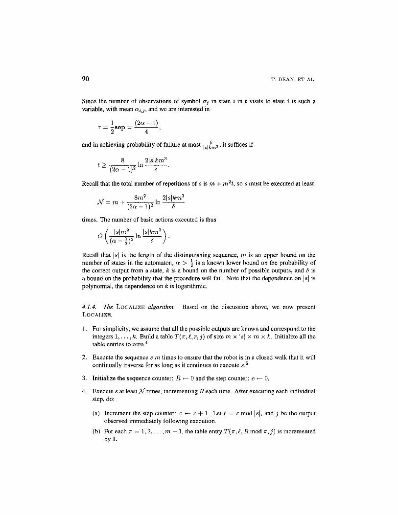
Since the number of observations of symbol a-j in state i in t visits to state i is such avariable, with mean otij, and we are interested in

and in achieving probability of failure at most . ,^ma, it suffices if

Recall that the total number of repetitions of s is m + m2t, so s must be executed at least

times. The number of basic actions executed is thus

Recall that \s\ is the length of the distinguishing sequence, m is an upper bound on thenumber of states in the automaton, a > \ is a known lower bound on the probability ofthe correct output from a state, k is a bound on the number of possible outputs, and 6 isa bound on the probability that the procedure will fail. Note that the dependence on s ispolynomial, the dependence on k is logarithmic.

4.1.4. The LOCALIZE algorithm. Based on the discussion above, we now presentLOCALIZE.

1. For simplicity, we assume that all the possible outputs are known and correspond to theintegers 1, . . . , k. Build a table T(TT, £, r, j) of size m x s\ x m x k. Initialize all thetable entries to zero.4

2. Execute the sequence s m times to ensure that the robot is in a closed walk that it willcontinually traverse for as long as it continues to execute s.5

3. Initialize the sequence counter: R <— 0 and the step counter: c <— 0.

4. Execute s at least A/" times, incrementing R each time. After executing each individualstep, do:

(a) Increment the step counter: c <— c + 1. Let £ = c mod s\, and j be the outputobserved immediately following execution.

(b) For each 7r = l ,2 , . . . ,m — 1, the table entry T(TT, f, R mod TT,J) is incrementedby 1.


5. Let

6. Let P be the LCM of all ir' such that there exist TT and i such that for all r < TTthere exists j such that F(ir,t,r,j) > | + |sep and i"' >s the period of the outputsarg maxj F(ir,£,r,j) for r = 0,1,...,IT — 1.

7. Conclude that the robot is currently located at the state corresponding to row r =R mod P in the main table for P, and return, as the hypothesis for the correct outputs ofthe distinguishing sequence s from this state, the sequence of outputs arg max, F(P, l, r,j) for £ = 0,1,..., | s|-l concatenated with the single output arg maxj F(P, 0, (r + 1)mod P, j).

4.2. The map learning procedure

Now we can define a procedure, BUILDMAP, for learning maps given a distinguishingsequence, s. Suppose for a moment that LOCALIZE always returns the robot to the samestate and that the robot can always determine when it is in a state that it has visited before.In this case, the robot can learn the connectivity of the underlying automaton by performingwhat amounts to a depth-first search through the automaton's state transition graph. Therobot does not actually traverse the state-transition graph in depth-first fashion; it cannotmanage a depth-first search since, in general, it cannot backtrack. Instead, it executessequences of actions corresponding to paths through the state transition graph starting fromthe root of the depth-first search tree by returning to the root each time using LOCALIZE.When, in the course of the search, a state is recognized as having been visited before, anappropriate arc is added to the inferred automaton and the search 'backtracks' to the nextpath that has not been completely explored.

The algorithm we present below is more complicated because our localization proceduredoes not necessarily always put the robot in the same final state and because we are notable to immediately identify the states we encounter during the depth-first search. The firstproblem is solved by performing many searches in parallel,6 one for each possible (root)state that LOCALIZE ends up in. Whenever the LOCALIZE is executed the robot knows(with high probability) what state it has landed in, and can take a step of the depth-firstsearch that has that state as the root node. The second problem is solved by using a numberof executions of the distinguishing sequence from a given starting state to identify that statewith high probability.

The algorithm, informally, proceeds in the following way. The robot runs LOCALIZE,ending in some state q. Associated with that state is a depth-first search which is in theprocess of trying to identify the node at the end of a particular path. The actions for that pathare executed, then the distinguishing sequence is executed. The results of the distinguishingsequence are tabulated, then the robot begins this cycle again with the localization procedure.Eventually, the current node in some search will have been explored enough times for a

92 T. DEAN, ET AL.

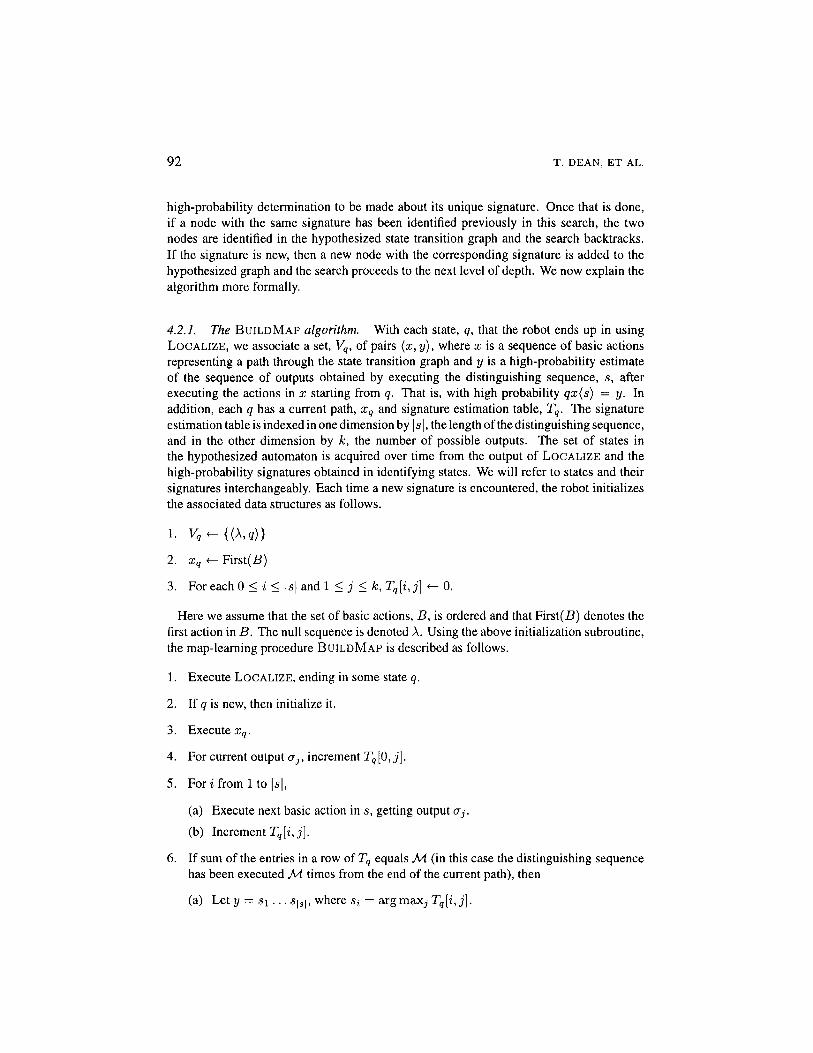
high-probability determination to be made about its unique signature. Once that is done,if a node with the same signature has been identified previously in this search, the twonodes are identified in the hypothesized state transition graph and the search backtracks.If the signature is new, then a new node with the corresponding signature is added to thehypothesized graph and the search proceeds to the next level of depth. We now explain thealgorithm more formally.

4.2.1. The BUILDMAP algorithm. With each state, q, that the robot ends up in usingLOCALIZE, we associate a set, Vq, of pairs (x, y), where x is a sequence of basic actionsrepresenting a path through the state transition graph and y is a high-probability estimateof the sequence of outputs obtained by executing the distinguishing sequence, s, afterexecuting the actions in x starting from q. That is, with high probability qx(s) = y. Inaddition, each q has a current path, xq and signature estimation table, Tq. The signatureestimation table is indexed in one dimension by s\, the length of the distinguishing sequence,and in the other dimension by k, the number of possible outputs. The set of states inthe hypothesized automaton is acquired over time from the output of LOCALIZE and thehigh-probability signatures obtained in identifying states. We will refer to states and theirsignatures interchangeably. Each time a new signature is encountered, the robot initializesthe associated data structures as follows.

1. Vq^{(X,q)}

2. xq <- First(S)

3. For each 0 < i < \s\ and 1 < j < k, T q [ i , j ] <- 0.

Here we assume that the set of basic actions, B, is ordered and that First(-B) denotes thefirst action in B. The null sequence is denoted A. Using the above initialization subroutine,the map-learning procedure BUILDMAP is described as follows.

1. Execute LOCALIZE, ending in some state q.

2. If q is new, then initialize it.

3. Execute xq.

4. For current output a^, increment Tq [0, j].

5. For i from 1 to |s|,

(a) Execute next basic action in s, getting output aj.

(b) Increment Tq [i, j].

6. If sum of the entries in a row of Tq equals M (in this case the distinguishing sequencehas been executed M times from the end of the current path), then

(a) Let y = s 1 . . . S|s|, where Si = argmax., T q [ i , j}.


(b) Add{z,,i/)toV,.

(c) If there is no other entry in Vq with signature equal to y, then set xq to the concate-nation of a;, and First(S), else backtrack by setting xq to the next unexplored pathin a depth-first search of Vq or return Vq if no such path exists.

(d) For all 0 < i < \s\ and 1 < j < k, T q [ i , j ] <- 0.

7. Go to Step 1.

4.2.2. Required number of steps. The above procedure will return the results of the firstdepth-first search that is finished. The returned Vq contains all of the information requiredto construct the state transition graph for the automaton with high probability assumingthat LOCALIZE succeeds with high enough probability and that the estimations used inidentifying states are correct with high enough probability. In the following, we show howto guarantee that these assumptions are satisfied.

The result of the depth-first search is correct if all of its arcs have been correctly identified.This requires at most m\B\ correct node identifications; one for executing each basic actionfrom each state.

A node is correctly identified if its signature is correctly determined, which will be thecase if each of its \s\ components is correct. A component of the final signature is correctwhenever the maximal frequency in the associated row of T is the one for the correct output.An individual observation of a signature element is correct if LOCALIZE succeeded (westarted where we think we started) and the state is perceived correctly; this will happen withprobability a/3, where /3 = 1 - 6 is the probability that LOCALIZE succeeds. In the worstcase, the next most likely element of the table will have expected frequency 1 - a/3, givinga separation between these two probabilities of 2a/9 - 1. The row will yield the correctanswer if all of its entries are within a/3-1/2 of their expected values. Using Hoeffding'sinequality as before, after M trials, the probability that an individual table element is inerror is bounded above by

In order to guarantee that the total error probability of the algorithm is less than rj, we mustensure that the error probability for a single table entry is less than r]/(\s\km\B\). This willbe the case if

At worst, we must perform \Q\ depth-first searches,7 each of which requires |Q||B| nodesto be identified.8 To identify a node, we must execute the distinguishing sequence there Mtimes. To do that requires JV + 1 executions of the distinguishing sequence; A/" of them tolocalize to the root of the search, plus 1 to identify the node. In addition, each attempt atnode identification requires the path to be followed from the root of the tree to the node; thelength of the path is bounded above by \Q\. Thus, the number of steps required is at most

94 T. DEAN, ET AL.

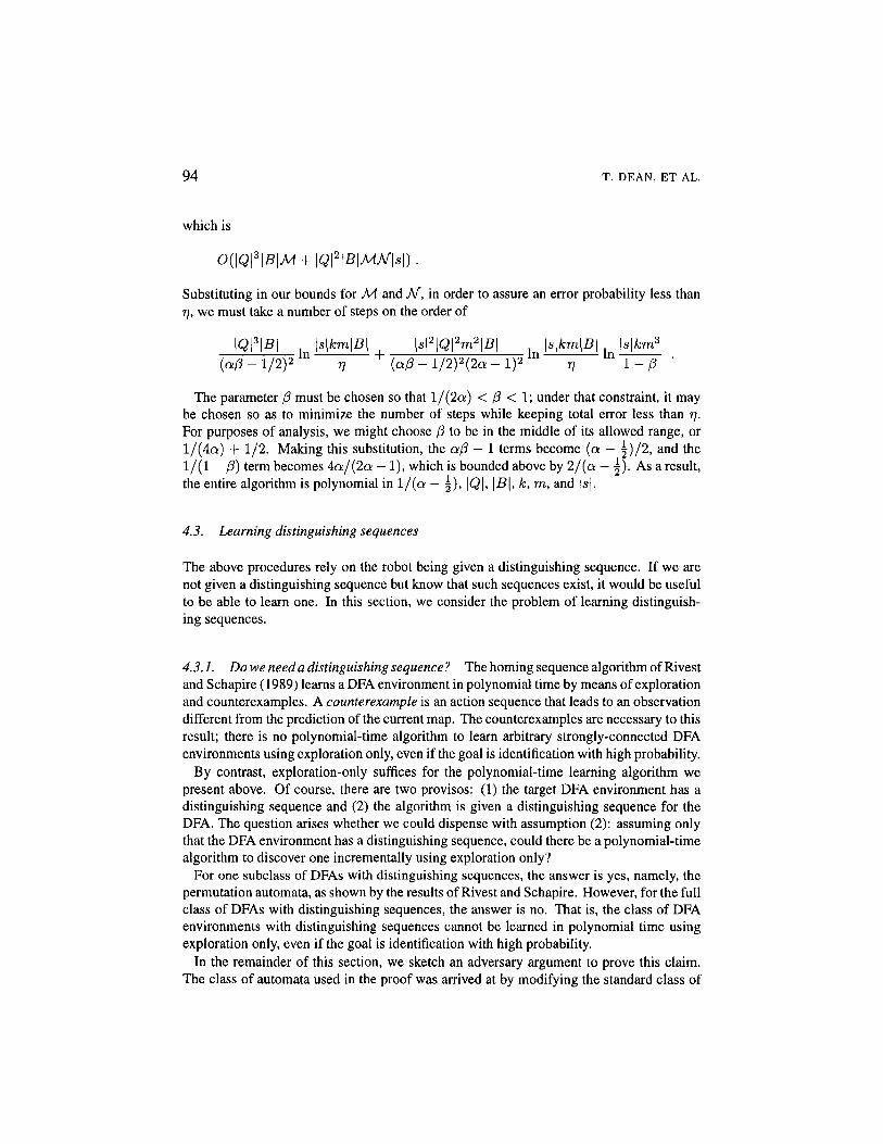
which is

Substituting in our bounds for M and M, in order to assure an error probability less thanr\, we must take a number of steps on the order of

The parameter /3 must be chosen so that l/(2cc) < /3 < 1; under that constraint, it maybe chosen so as to minimize the number of steps while keeping total error less than r\.For purposes of analysis, we might choose 0 to be in the middle of its allowed range, orl/(4a) + 1/2. Making this substitution, the a/3 - 1 terms become (a - \)/1, and the1/(1 - (3) term becomes 4a/(2a - 1), which is bounded above by 2/(a - |). As a result,the entire algorithm is polynomial in l/(a - 5), \Q\, \B\, k, m, and |s|.

4.3. Learning distinguishing sequences

The above procedures rely on the robot being given a distinguishing sequence. If we arenot given a distinguishing sequence but know that such sequences exist, it would be usefulto be able to learn one. In this section, we consider the problem of learning distinguish-ing sequences.

4.3.1. Do we need a distinguishing sequence ? The homing sequence algorithm of Rivestand Schapire (1989) learns a DFA environment in polynomial time by means of explorationand counterexamples. A counterexample is an action sequence that leads to an observationdifferent from the prediction of the current map. The counterexamples are necessary to thisresult; there is no polynomial-time algorithm to learn arbitrary strongly-connected DFAenvironments using exploration only, even if the goal is identification with high probability.

By contrast, exploration-only suffices for the polynomial-time learning algorithm wepresent above. Of course, there are two provisos: (1) the target DFA environment has adistinguishing sequence and (2) the algorithm is given a distinguishing sequence for theDFA. The question arises whether we could dispense with assumption (2): assuming onlythat the DFA environment has a distinguishing sequence, could there be a polynomial-timealgorithm to discover one incrementally using exploration only?

For one subclass of DFAs with distinguishing sequences, the answer is yes, namely, thepermutation automata, as shown by the results of Rivest and Schapire. However, for the fullclass of DFAs with distinguishing sequences, the answer is no. That is, the class of DFAenvironments with distinguishing sequences cannot be learned in polynomial time usingexploration only, even if the goal is identification with high probability.

In the remainder of this section, we sketch an adversary argument to prove this claim.The class of automata used in the proof was arrived at by modifying the standard class of


'password automata' to have distinguishing sequences without compromising their 'cryp-tographic' attributes. This shows that our algorithm will not be able to do entirely withouta distinguishing sequence. However, in the next section we show how to use a randomgenerator of sequences that produces correct distinguishing sequences only some small (atleast inverse polynomial) fraction of the time.

Lemma 1. Any algorithm that can learn the class of DFA environments with distinguishingsequences by exploration only will take exponential time on some environments, even if thegoal is identification with high probability and a reset operation is available.

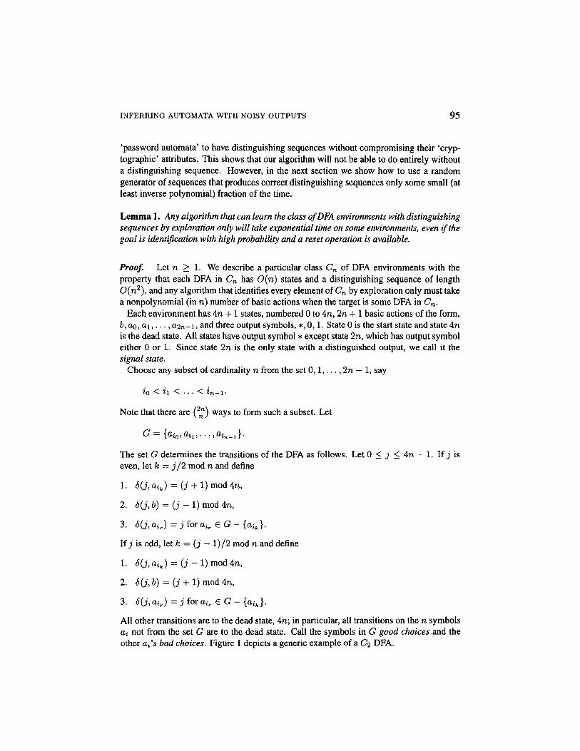
Proof. Let n > 1. We describe a particular class Cn of DFA environments with theproperty that each DFA in Cn has O(n) states and a distinguishing sequence of lengthO(n2), and any algorithm that identifies every element of Cn by exploration only must takea nonpolynomial (in n) number of basic actions when the target is some DFA in Cn.

Each environment has 4n +1 states, numbered 0 to 4n, 2n + 1 basic actions of the form,6, a0, a 1 , . . . , a2n-1, and three output symbols, *, 0,1. State 0 is the start state and state 4nis the dead state. All states have output symbol * except state 2n, which has output symboleither 0 or 1. Since state 2n is the only state with a distinguished output, we call it thesignal state.

Choose any subset of cardinality n from the set 0 ,1 , . . . , 2n — 1, say

Note that there are (2^) ways to form such a subset. Let

The set G determines the transitions of the DFA as follows. Let 0 < j < 4n — 1. If j iseven, let k = j/2 mod n and define

1 • <5(j, aik) = (j + 1) mod 4n,

2. 6(j,b) = ( j - l )mod4n,

3. 6(j, air) = j for air € G - {aik}.

If j is odd, let k = (j — l)/2 mod n and define

1. 6(j, ^ J = (j - 1) mod 4n,

2. 6(j, 6) = (j + 1) mod 4n,

3. 6(j, air) = j for air 6 G - {aik}.

All other transitions are to the dead state, 4n; in particular, all transitions on the n symbolsa, not from the set G are to the dead state. Call the symbols in G good choices.and theother flj's bod choices. Figure 1 depicts a generic example of a C2 DFA.

96 T. DEAN, ET AL.

Figure 1. Generic example of Cz DFA. Gc denotes the set of bad choices.

Intuitively, the 4n non-dead states form a ring that can be traversed from the start state 0in increasing order back to the start state by the string

and in the reverse direction by the string

The left half of either of these strings will proceed from the start state to the signal state, In.Note that symbols aik that are good choices either move one state around the ring or stay

in the same state. Hence the string

starting from an even numbered state j in the ring moves around the ring in increasingorder until it comes back to j. If we execute d starting from an odd numbered state j, wemove around the ring in decreasing order until we come back to j. Since in either case weare bound to encounter the signal state in a unique location in the string, the string d is adistinguishing sequence for this DFA. (Note that if we execute d from the dead state, wedo not encounter the signal state at all.) The length of d is O(n2).

Thus, every DFA environment in the class Cn has a distinguishing string, determinedby the corresponding set G. Intuitively, what prevents us from using this information to


learn elements of the class Cn? If we are given an unknown element of Cn, we do notknow G, that is, which subset of n of the 2n symbols ctj are "good choices." If we try toguess this information, we are liable to include a "bad choice" that will leave us in the deadstate capable of gathering no more useful information until we issue a reset. Moreover, toidentify the environment, we must visit the signal state, which means we have to executeall and only the "good choices" appropriately interspersed with 6's.

These intuitions may be turned into an adversary argument as follows. Suppose A isan algorithm that identifies with high probability every environment in Cn by explorationonly, possibly using resets. The adversary will simulate A, returning certain observationsin response to the successive basic actions executed by A. The adversary gets to pickthe DFA subject to its being consistent with the observations it has already returned. Theadversary keeps track of the set T of possible environments, as well as the current state ofthe learning algorithm in each one. Initially T contains all the elements of Cn, each one inits initial state.

In response to each basic action executed by A, the adversary updates the current state ofA for each element of T. As long as there are more than two elements of T, the adversaryreturns the observation * and removes from T any DFAs that don't have output * at thecurrent state. If there are only two elements of T, then if they both have the same output attheir current states, the adversary returns that observation to A. Otherwise, the two DFAshave different outputs, and the adversary selects one of them and answers consistent withthat one for all remaining actions.

Note that for every choice of G, there are two corresponding DFAs in Cn that have thesame transition function and only differ in the output (0 or 1) from the signal state; anysequence of actions from A will reach the same state in both machines. How many DFAscan be eliminated from T by an observation of *? We claim the answer is at most two. Tobe eliminated, a DFA must be in its signal state. But, for a DFA corresponding to G to be inits signal state, the sequence of actions since the last reset (or the beginning of the sequence,if there have been no resets) must contain all of the actions from G and no action aj not inG. Since this condition cannot be satisfied simultaneously for two distinct sets G, at mostthe two DFAs corresponding to a single G can be eliminated from T by an observation of *.

If the algorithm A gives its output before T is reduced to one element, then it must makean error when the target environment is at least one of the elements of T. This shows thatany deterministic algorithm A that successfully identifies every element of Cn must, whenthe target is some element of Cn, execute enough basic actions to eliminate all but oneelement of Cn; this requires at least 2" basic actions, since (2^) is bounded below by 2n.

If the algorithm A is randomized we consider the possible runs of A against the adversarydescribed above until A halts. Let T be the random variable that is the value of T when Ahalts. If the probability that A executes more than 2n-1 basic actions before it halts is atleast one half, we are done. Otherwise, consider the runs in which A halts before executing2™"1 basic actions. For these runs, T contains more than half the elements of Cn. Thus,if we consider instead an adversary that chooses uniformly at random a DFA from Cn andreturns observations consistent with that DFA, the probability is at least 1/4 that the outputof A will be different from the chosen DFA. Thus, A does not succeed in identification withhigh probability. D

98 T. DEAN, ET AL.

If it is desired that the target DFAs be strongly connected, it suffices to add the "reset"as a basic action, to take the DFAs back to their start states. Note that in the constructionabove, the number of basic actions is proportional to the number of states, or "places."What if the number of basic actions is bounded by a constant? A somewhat more elaborateconstruction shows that even in this case the class of DFAs with distinguishing sequencescannot be learned in polynomial time using exploration only. The key idea is to use binarycoding for the symbols aj, guaranteeing that the new states necessary to implement thecoding have outputs that distinguish them "locally" - still requiring the correct sequence of"good choices" to distinguish them globally. The details of this refinement are omitted.

4.3.2. Using a 'weak' distinguishing sequence oracle. In the last section, we showedthat, in general, without either a source of counterexamples or a distinguishing sequencewe cannot learn a DFA in polynomial time. However, all is not lost. Suppose that we aregiven an oracle that generates candidate distinguishing sequences, such that it (a) generatessequences s of length at most •$, polynomial in |Q|, and (b) generates correct distinguishingsequences with probability 1 — C« bounded below by an inverse polynomial in |Q|. Weassume that sequences are generated independently. Then we define a procedure that, giventwo different candidate maps of the environment, determines with high probability which,if either, is in fact the correct map. That is, the procedure fails iff at least one of its inputs isa correct map and it outputs an incorrect map. We then use the oracle to generate a seriesof possible distinguishing sequences. Each sequence is used to build a map, which is thencompared against the current candidate map; the 'better' one is kept as the new candidate.If enough such comparisons are performed, we can ensure that the output of this procedureis a correct map of the environment (and its generating sequence a distinguishing sequence)with high probability (1 - £). We describe the procedure in more detail below.

First, we develop the procedure COMPARE for comparing two different maps that choosesa correct map for the environment with probability at least 1 — K. Given two non-equivalentDFAs and the current state of the robot in each, q\ and q-2, a sequence of inputs a (adiscriminating sequence) can be generated (in polynomial time) such that ~i(q\a) ^ 7(92^)-|a| is bounded by the product of the sizes of the two DFAs (and thus, by m2). Thus, after weexecute a, at least one of the DFAs will predict an output different from that observed. Acorrect DFA will predict the observed output with probability at least a, while the incorrectmap will do so with at most 1 - a probability. Hence, we repeatedly generate and executediscriminating sequences, incrementally maintaining a record of each DFA's frequency ofprediction error. If we perform enough such trials, if either DFA is correct, it will be theone with the lower estimated prediction error (with high probability). We need to performenough trials so that the estimated frequency of prediction error is within \ (a - \) of the truevalue, with probability at least 1 - K. We can now derive V, the number of discriminationsneeded to do a successful comparison with probability at least 1 — K. Using the Hoeffdingbounds as previously, we get


COMPARE is invoked with two triples, i.e., COMPARE((Mj, 91, si), (M2, q2, s 2 ) ) , eachconsisting of an automaton, the current state of the robot in that automaton, and a distin-guishing sequence used in constructing that automaton. The procedure returns one of thetwo triples.

1. ni <— ri2 <— 0.

2. Repeat Z> times:

(a) If M1 starting at 91 is equivalent to M2 starting at q2. then return (Mi,9i,si);

(b) Else:

i. Find a discriminating sequence a such that 7(910) ^ 7(92^).ii. Execute a and observe output y.

iii. If y ^ 7(910), HI <- ni + 1.

iv. If y / 7(920), n2 <— n2 + 1.

v. q1 <— q1l. 92 <— 920-

3. If n1 < n2, return (Mi, 9i,si);

4. Else return (M2,92,52).

Now, given this comparison procedure and a distinguishing sequence oracle as describedabove, we can determine the number of comparisons C needed to ensure that with probabilityat least 1 — £ the map output is correct (and its generating sequence is a distinguishingsequence). We first get bounds on the probability of not getting a correct map output, givenC comparisons (we assume an initial map is generated first). The probability of a singlemap-building step not resulting in a correct map is < C+(1~C)T? = 1-(1-??)(1—0>, sinceeither the sequence used was not a distinguishing sequence (the oracle 'failed'), or it was andthe map-building step failed. Note that each map-building step is assumed to be independentfrom the others (as provided by the algorithm described above). Thus, the probability of notgenerating a correct map over C trials is bounded by (1 - (1 - ij)(l - £))c. The probabilityof not accepting a correct map in some comparison is bounded by K£. Hence, the totalprobability of failure is bounded by (1 - (1 — 77) (1 - Q)c + K,C. We now wish to chooseC so that this probability is less than £. We do this by finding bounds that cause each termto be less than |. First, we get a lower bound on C:

It suffices if

100 T. DEAN, ET AL.

Given this lower bound on C, we can determine an upper bound on K so that C comparisonssuffice. We have:

We can now substitute our bound for K to get a complete bound for T>:

The total number of exploration steps required is determined by C + 1 invocations ofBUILDMAP plus C invocations of COMPARE, each requiring at most D executions ofaction sequences of length at most m2. Thus, using the bound for BUILDMAP givenabove, we have a (loose) bound on the number of primitive actions required to identify anautomaton with high probability,

which is polynomial in the relevant variables. Note that, like b for BUILDMAP, 77 is a freeparameter that may be chosen to minimize the number of steps taken. Intuitively, we canallow each map to be less probably correct, if we check more of them. Of course, 77 mustbe inverse polynomial in the number of DFA states.

The complete procedure for learning map with high probability given an oracle for gen-erating distinguishing sequences is described below, where BUILDMAP is assumed to takea distinguishing sequence as input and return as output an automaton and the current stateof the robot in that automaton.

1. s1— oracle output.

2. ( M 1 , q 1 ) <- BUILDMAP(SI).

3. Repeat C times:

(A) S2 <— oracle output.

(B) (M2,q2) <-BUILDMAP(s2).

(C) (Mitqi,si) *-COMPARE({Mi,qr1,Si),(M2)g2,S2»

4. Return (Mi,qi,si).


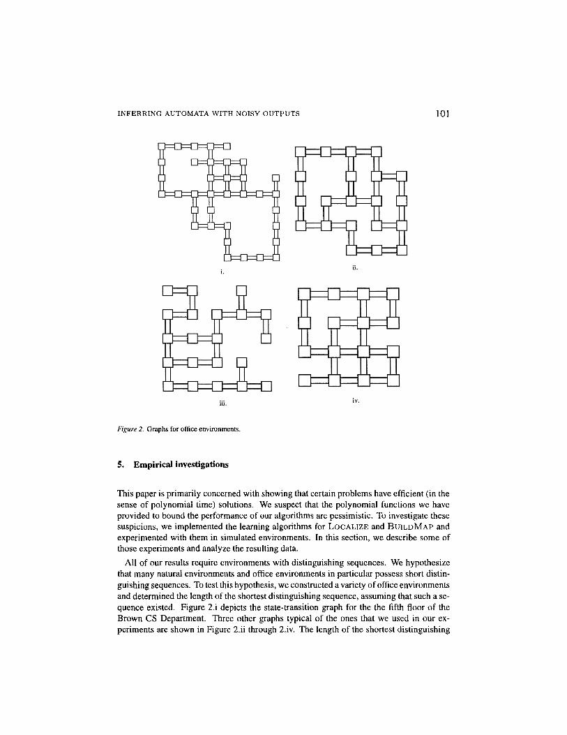
Figure 2. Graphs for office environments.

5. Empirical investigations

This paper is primarily concerned with showing that certain problems have efficient (in thesense of polynomial time) solutions. We suspect that the polynomial functions we haveprovided to bound the performance of our algorithms are pessimistic. To investigate thesesuspicions, we implemented the learning algorithms for LOCALIZE and BUILDMAP andexperimented with them in simulated environments. In this section, we describe some ofthose experiments and analyze the resulting data.

All of our results require environments with distinguishing sequences. We hypothesizethat many natural environments and office environments in particular possess short distin-guishing sequences. To test this hypothesis, we constructed a variety of office environmentsand determined the length of the shortest distinguishing sequence, assuming that such a se-quence existed. Figure 2.i depicts the state-transition graph for the the fifth floor of theBrown CS Department. Three other graphs typical of the ones that we used in our ex-periments are shown in Figure 2.ii through 2.iv. The length of the shortest distinguishing

102 T. DEAN, ET AL.

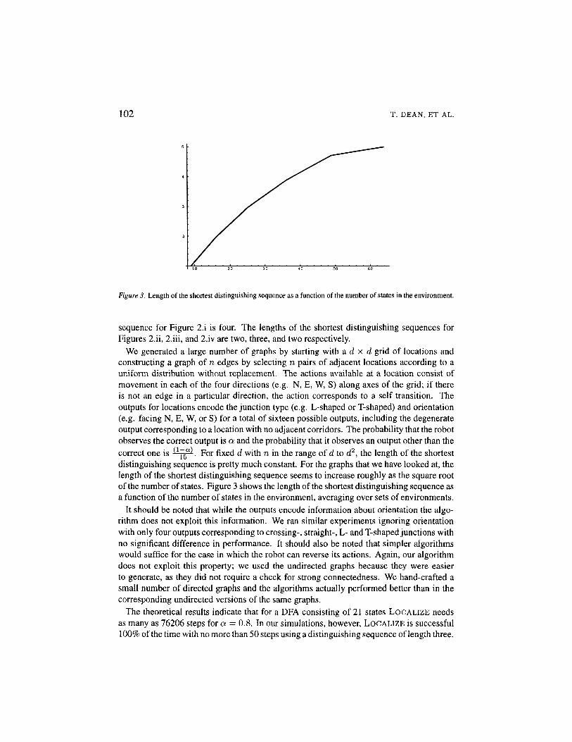
Figure 3. Length of the shortest distinguishing sequence as a function of the number of states in the environment.

sequence for Figure 2.i is four. The lengths of the shortest distinguishing sequences forFigures 2.ii, 2.iii, and 2.iv are two, three, and two respectively.

We generated a large number of graphs by starting with a d x d grid of locations andconstructing a graph of n edges by selecting n pairs of adjacent locations according to auniform distribution without replacement. The actions available at a location consist ofmovement in each of the four directions (e.g. N, E, W, S) along axes of the grid; if thereis not an edge in a particular direction, the action corresponds to a self transition. Theoutputs for locations encode the junction type (e.g. L-shaped or T-shaped) and orientation(e.g. facing N, E, W, or S) for a total of sixteen possible outputs, including the degenerateoutput corresponding to a location with no adjacent corridors. The probability that the robotobserves the correct output is a and the probability that it observes an output other than thecorrect one is 15 . For fixed d with n in the range of d to d2, the length of the shortestdistinguishing sequence is pretty much constant. For the graphs that we have looked at, thelength of the shortest distinguishing sequence seems to increase roughly as the square rootof the number of states. Figure 3 shows the length of the shortest distinguishing sequence asa function of the number of states in the environment, averaging over sets of environments.

It should be noted that while the outputs encode information about orientation the algo-rithm does not exploit this information. We ran similar experiments ignoring orientationwith only four outputs corresponding to crossing-, straight-, L- and T-shaped junctions withno significant difference in performance. It should also be noted that simpler algorithmswould suffice for the case in which the robot can reverse its actions. Again, our algorithmdoes not exploit this property; we used the undirected graphs because they were easierto generate, as they did not require a check for strong connectedness. We hand-crafted asmall number of directed graphs and the algorithms actually performed better than in thecorresponding undirected versions of the same graphs.

The theoretical results indicate that for a DFA consisting of 21 states LOCALIZE needsas many as 76206 steps for a — 0.8. In our simulations, however, LOCALIZE is successful100% of the time with no more than 50 steps using a distinguishing sequence of length three.


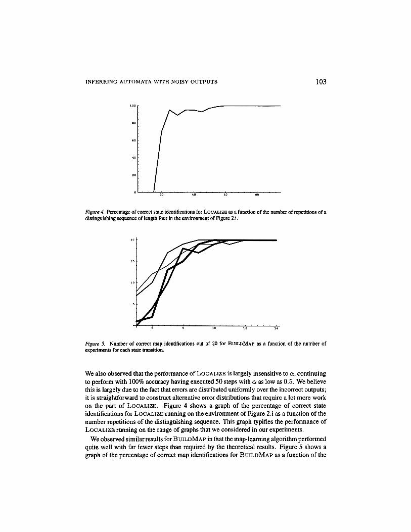
Figure 4. Percentage of correct state identifications for LOCALIZE as a function of the number of repetitions of adistinguishing sequence of length four in the environment of Figure 2.i.

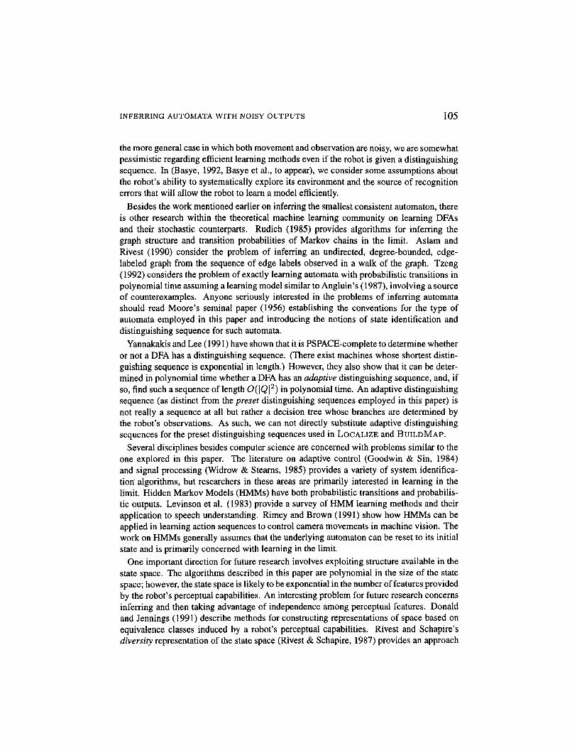
Figure 5. Number of correct map identifications out of 20 for BUILDMAP as a function of the number ofexperiments for each state transition.

We also observed that the performance of LOCALIZE is largely insensitive to a, continuingto perform with 100% accuracy having executed 50 steps with a as low as 0.5. We believethis is largely due to the fact that errors are distributed uniformly over the incorrect outputs;it is straightforward to construct alternative error distributions that require a lot more workon the part of LOCALIZE. Figure 4 shows a graph of the percentage of correct stateidentifications for LOCALIZE running on the environment of Figure 2.i as a function of thenumber repetitions of the distinguishing sequence. This graph typifies the performance ofLOCALIZE running on the range of graphs that we considered in our experiments.

We observed similar results for BUILDMAP in that the map-learning algorithm performedquite well with far fewer steps than required by the theoretical results. Figure 5 shows agraph of the percentage of correct map identifications for BUILDMAP as a function of the

104 T. DEAN, ET AL.

Figure 6. Comparison of BUILDMAP running on directed and undirected versions of the same graph.

number of experiments performed for gathering statistics to infer each state transition. Thefour lines in Figure 5 correspond to the four graphs in Figure 2 with BUILDMAP generallyconverging more quickly the smaller the graph.

As mentioned earlier, BUILDMAP achieves no advantage from the fact that our samplegraphs are undirected. Figure 6 compares the performance of BUILDMAP running ondirected and undirected versions of the same graph. The dashed line corresponds to theundirected graph. In this and similar cases, BUILDMAP actually performed better on thedirected versions of undirected graphs.

In the process of experimenting with BUILDMAP, we discovered a simple modificationto the algorithm that improves both the theoretical and empirical performance markedly.Executing the distinguishing sequence tends to force the robot into a subset of the set ofall states; we refer to the states that the robot ends up in after executing a distinguishingsequence as sinks. For instance, there are six sinks for the automaton shown in Figure 2.iiigiven a particular distinguishing sequence of length three. If there is a single sink or therobot always ends up in the same sink, then the robot will construct a single depth-firstsearch tree of size \Q\. In practice, however, the robot tends to bounce back and forthbetween sinks, constructing several depth-first search trees each of which may grow tosome significant percentage of \Q\ before one of the trees is complete. Much of the workin constructing the final automaton can be duplicated in constructing different search trees.Since the output of the distinguishing sequence provides a unique signature, the robot canconstruct a global table of signatures summarizing the information in all of the searchtrees and thus avoid duplicating search effort. Statistics gathered in one search tree can becombined with statistics gathered in another.

6. Related work

In this paper, we focus on the case in which movement is certain and observation is noisy, andshow how a robot might exploit the determinism in movement to enable efficient learning. In


the more general case in which both movement and observation are noisy, we are somewhatpessimistic regarding efficient learning methods even if the robot is given a distinguishingsequence. In (Basye, 1992, Basye et al., to appear), we consider some assumptions aboutthe robot's ability to systematically explore its environment and the source of recognitionerrors that will allow the robot to learn a model efficiently.

Besides the work mentioned earlier on inferring the smallest consistent automaton, thereis other research within the theoretical machine learning community on learning DFAsand their stochastic counterparts. Rudich (1985) provides algorithms for inferring thegraph structure and transition probabilities of Markov chains in the limit. Aslam andRivest (1990) consider the problem of inferring an undirected, degree-bounded, edge-labeled graph from the sequence of edge labels observed in a walk of the graph. Tzeng(1992) considers the problem of exactly learning automata with probabilistic transitions inpolynomial time assuming a learning model similar to Angluin's (1987), involving a sourceof counterexamples. Anyone seriously interested in the problems of inferring automatashould read Moore's seminal paper (1956) establishing the conventions for the type ofautomata employed in this paper and introducing the notions of state identification anddistinguishing sequence for such automata.

Yannakakis and Lee (1991) have shown that it is PSPACE-complete to determine whetheror not a DFA has a distinguishing sequence. (There exist machines whose shortest distin-guishing sequence is exponential in length.) However, they also show that it can be deter-mined in polynomial time whether a DFA has an adaptive distinguishing sequence, and, ifso, find such a sequence of length O(|Q|2) in polynomial time. An adaptive distinguishingsequence (as distinct from the preset distinguishing sequences employed in this paper) isnot really a sequence at all but rather a decision tree whose branches are determined bythe robot's observations. As such, we can not directly substitute adaptive distinguishingsequences for the preset distinguishing sequences used in LOCALIZE and BUILDMAP.

Several disciplines besides computer science are concerned with problems similar to theone explored in this paper. The literature on adaptive control (Goodwin & Sin, 1984)and signal processing (Widrow & Stearns, 1985) provides a variety of system identifica-tion algorithms, but researchers in these areas are primarily interested in learning in thelimit. Hidden Markov Models (HMMs) have both probabilistic transitions and probabilis-tic outputs. Levinson et al. (1983) provide a survey of HMM learning methods and theirapplication to speech understanding. Rimey and Brown (1991) show how HMMs can beapplied in learning action sequences to control camera movements in machine vision. Thework on HMMs generally assumes that the underlying automaton can be reset to its initialstate and is primarily concerned with learning in the limit.

One important direction for future research involves exploiting structure available in thestate space. The algorithms described in this paper are polynomial in the size of the statespace; however, the state space is likely to be exponential in the number of features providedby the robot's perceptual capabilities. An interesting problem for future research concernsinferring and then taking advantage of independence among perceptual features. Donaldand Jennings (1991) describe methods for constructing representations of space based onequivalence classes induced by a robot's perceptual capabilities. Rivest and Schapire'sdiversity representation of the state space (Rivest & Schapire, 1987) provides an approach

106 T. DEAN, ET AL.

to reducing the storage required in representing automata. Bachrach (1992) shows howto implement Rivest and Schapire's learning algorithm in a connectionist architecture. Insome problems, it is advantageous for a representation to coalesce distinct environmentalstates that require the same response from the robot. Whitehead and Ballard (1991) dealwith the problems that arise in reinforcement learning when perception maps different statesto the same internal representation.

7. Conclusions

In this paper, we provide general methods for the inference of finite automata with stochasticoutput functions. We demonstate that it is possible to exploit determinism in movement toenable efficient learning. In previous work (Basye & Dean, 1989, Basye et al., 1989), weconcentrated on problems in which the state transition function is stochastic (e.g., in thecontext of map learning, this means that the robot's navigation procedures are prone to error).In future work, we intend to combine our results to handle uncertainty in both movementand observation. We are also interested in identifying and exploiting additional structureinherent in real environments (e.g., office environments represent a severely restricted classof planar graphs) and in exploring more forgiving measures of performance (e.g., it isseldom necessary to learn about the entire environment as long as the robot can navigateefficiently between particular locations of interest).

With regard to more forgiving measures of performance, it may be possible to extend thetechniques of this paper to find e-approximations rather than exact solutions by using theprobably approximately correct learning model of Valiant (1984). Such extensions wouldrequire the introduction of a distribution, Pr, governing both performance evaluation andexploration. As one simple example, suppose that the robot operates as follows. Periodicallythe robot is asked to execute a particular sequence of actions chosen according to Pr; weassume that, prior to being asked to execute the sequence, it has performed localizationand that immediately following it executes the distinguishing sequence. Performance ismeasured in terms of the robot's ability to plan paths between locations identified by theirdistinguishing sequence signatures, where the paths are generated according to Pr. Theproblem with this approach is that the starting locations of the sequences are not determinedsolely by Pr. In fact, all that Pr governs is Pr(s|<7start). where <?start is the start state. In orderfor the above approach to work, the marginal distribution governing the possible startinglocations of the robot, Pr(gstart), must be the same for both training and performanceevaluation. In future research, we will be exploring a number of different approaches tospecifying e-approximations.

Acknowledgments

This work was supported in part by a National Science Foundation Presidential YoungInvestigator Award IRI-8957601, by the Air Force and the Advanced Research ProjectsAgency of the Department of Defense under Contract No. F30602-91-C-0041, and by theNational Science foundation in conjunction with the Advanced Research Projects Agency


of the Department of Defense under Contract No. IRI-8905436. Dana Angluin is supportedby NSF Grant CCR-9014943. Sean Engelson is supported by the Fannie and John HertzFoundation.

Notes

1. There has to be some requirement on the size of the DFA, otherwise the robot could choose the DFA corre-sponding to the complete chain of inputs and outputs.

2. In (Basye, 1992, Basye et al., to appear), we consider a more efficient approach for the case in which 7 isunambiguous which, under more restrictive conditions than those required in this paper, infers the underlyingautomaton by estimating the transition probabilities on the observed states (i.e., the probability of observing inext given that the robot observed j last).

3. The arguments in this paper require that a > \ and they exploit the separation between a and ̂ . Itappears to be straightforward to relax this requirement somewhat. Let Pij be the probability of observingoutput j/j given that the robot is in the state <ft. Let Pi = maxj{Py}. We assume that there exists oneoutput that is observed more frequently than any other (i.e., if Pij = Pik = P* then j = k). Let Sj bethe difference between the most frequently observed and the second most frequently observed outputs (i.e.,Si = minj{Pi* — Pij\P? < Pij}), and s be a lower bound on the si (i.e., s = minj{si}). We see noobstacle (other than a slightly more complicated proof) to extending our arguments to work with a separationof s. We have observed empirically that the algorithms described in this paper work well without modificationin many cases in which a < |.

4. If the outputs are not known, then the table can be constructed incrementally, adding new outputs as theyare observed.

5. Following Step 2, the next action should be the first action in a.

6. The idea of using multiple searches starting from the states resulting from LOCALIZE is similar to the way inwhich Rivest and Schapire (1989) run multiple versions of Angluin's L* algorithm (Angluin, 1987) startingfrom the states the robot ends up in after executing a given homing sequence.

7. Note that we must use m, an a priori bound on the number of state in order to choose M and A/" to guaranteea certain level of confidence. The number of nodes that are identified in the depth-first search need not beestimated in advance, however, so we use \Q\, the actual size of the state space here, rather than m.

8. In the BUILDMAP algorithm presented here, a number of searches may be carried out in parallel, potentiallyduplicating work unecessarily. In fact, though, the different depth-first searches need not be treated as inde-pendent; a global signature table can be constructed by the separate searches working together. This removesa factor of \Q\ from the number of steps required, but complicates the algorithm somewhat.

References

Angluin, D. (1978). On the complexity of minimum inference of regular sets. Information and Control 39:337-350.

Angluin, D. (1987). Learning regular sets from queries and counterexamples. Information and Computation75:87-106.

Aslam, J.A., & Rivest, R.L. (1990). Inferring graphs from walks. In Proceedings COLT-88.Bachrach, J.R. (1992). Connectionist modeling and control of finite state environments. Technical Report 92-6,

University of Massachusetts at Amherst Department of Computer and Information Science.Basye, K., & Dean, T. (1989). Map learning with indistinguishable locations. In Proceedings of the Fifth Workshop

on Uncertainty in Al. 7-13.Basye, K., Dean, T, & Vitter, J.S. (1989). Coping with uncertainty in map learning. In Proceedings IJCAI11.

IJCAII. 663-668.Basye, K., Dean, T, & Kaelbling, L. (to appear). Learning dynamics: System identification for perceptually

challenged agents. Artificial Intelligence.

108 T. DEAN, ET AL.

Basye, K. (1992). A framework for map construction. Technical report. Brown University Department ofComputer Science, Providence, RI.

Dean, T., Basye, K., Chekaluk, R., Hyun, S., Lejter, M., & Randazza, M. (1990). Coping with uncertainty in acontrol system for navigation and exploration. In Proceedings AAAI-90. AAAI. 1010-1015.

Donald, B., & Jennings, J. (1991). Sensor interpretation and task-directed planning using perceptual equivalenceclasses. Technical Report CU-CS-TR, Cornell University Computer Science Department.

Dudek, G., Jenkins, M., Milios, E., & Wilkes, D. (1988). Robotic exploration as graph construction. TechnicalReport RBCV-TR-88-23, University of Toronto.

Gold, E.M. (1972). System identification via state characterization. Automatica 8:621-636.Gold, E.M. (1978). Complexity of automaton identification from given sets. Information and Control 37:302-320.Goodwin, G.C., & Sin, K.S. (1984). Adaptive Filtering Prediction and Control. Prentice-Hall, Englewood Cliffs,

New Jersey.Kaelbling, L., Basye, K., Dean, T., Kokkevis, E., & Maron, O. (1992). Robot map-learning as learning labeled

graphs from noisy data. Technical Report CS-92-15, Brown University Department of Computer Science.Kearns, M., & Valiant, L.G. (1989). Cryptographic limitations on learning boolean functions and finite automata.

In Proceedings of the Twenty First Annual ACM Symposium on Theoretical Computing. 433-444.Kuipers, B.J., & Byun, Y.-T. (1988). A robust, qualitative method for robot spatial reasoning. In Proceedings

AAAI-88. AAAI. 774-779.Kuipers, B. (1978). Modeling spatial knowledge. Cognitive Science 2:129-153.Levinson, S.E., Rabiner, L.R., & Sondhi, M.M. (1983). An introduction to the application of the theory of

probabilistic functions of a Markov process to automatic speech recognition. The Bell System Technical Journal62(4):1035-1074.

Levitt, T.S., Lawton, D.T., Chelberg, D.M., & Nelson, P.C. (1987). Qualitative landmark-based path planning andfollowing. In Proceedings AAAI-87. AAAI. 689-694.

Moore, E.F. (1956). Gedanken-experiments on sequential machines. In Automata Studies. Princeton UniversityPress, Princeton, New Jersey. 129-153.

Pitt, L., & Warmuth, M.K. (1989). The minimum consistent DFA problem cannot be approximated within anypolynomial. In Proceedings of the Twenty First Annual ACM Symposium on Theoretical Computing. 421-432.

Rimey, R.D., & Brown, C.M. (1991). Controlling eye movements with hidden Markov models. InternationalJournal of Computer Vision 7(l):47-65.

Rivest, R.L., & Schapire, R.E. (1987). Diversity-based inference of finite automata. In Proceedings of the TwentyEighth Annual Symposium on Foundations of Computer Science. 78-87.

Rivest, R.L., & Schapire, R.E. (1989). Inference of finite automata using homing sequences. In Proceedings ofthe Twenty First Annual ACM Symposium on Theoretical Computing. 411 -420.

Rudich, S. (1985). Inferring the structure of a Markov chain from its output. In Proceedings of the Twenty SixthAnnual Symposium on Foundations of Computer Science. 321-326.

Schapire, R.E. (1991). The design and analysis of efficient learning algorithms. Technical Report MIT/LCS/TR-493, MIT Laboratory for Computer Science.

Tzeng, W.-G. (1992). Learning probabilistic automata and Markov chains via queries. Machine Learning 8:151-166.

Valiant, L.G. (1984). A theory of the leamable. Communications of the ACM 27:1134-1142.Whitehead, S.D., & Ballard, D.H. (1991). Learning to perceive and act by trial and error. Machine Learning 1.Widrow, B., & Stearns, S.D. (1985). Adaptive Signal Processing. Prentice-Hall, Englewood Cliffs, N.J.Yannakakis, M., &Lee, D. (1991). Testing finite state machines. In ACM Symposium on Theoretical Computing.

ACM Press. 476-485.

Received December 13, 1993Accepted April 11, 1994Final Manuscript April 21, 1994

inferring finite automata with stochastic output functions … · · 2017-08-25inferring finite...

Documents