Face and Landmark Detection by Using Cascade of Classifiers

Hakan CevikalpEskisehir Osmangazi University

Eskisehir, Turkeyhakan.cevikalp@gmail.com

Bill TriggsLaboratoire Jean Kuntzmann

Grenoble Cedex 9, FranceBill.Triggs@imag.fr

Vojtech FrancCzech Technical University

Praha, Czech Republicxfrancv@cmp.felk.cvut.cz

Abstract— In this paper, we consider face detection alongwith facial landmark localization inspired by the recent studiesshowing that incorporating object parts improves the detectionaccuracy. To this end, we train roots and parts detectors wherethe roots detector returns candidate image regions that coverthe entire face, and the parts detector searches for the landmarklocations within the candidate region. We use a cascade ofbinary and one-class type classifiers for the roots detectionand SVM like learning algorithm for the parts detection. Ourproposed face detector outperforms the most of the successfulface detection algorithms in the literature and gives the secondbest result on all tested challenging face detection databases.Experimental results show that including parts improves thedetection performance when face images are large and thedetails of eyes and mouth are clearly visible, but does notintroduce any improvement when the images are small.

I. INTRODUCTIONIn recent years, face detection has been thoroughly studied

due to its wide potential applications, including face recog-nition, human-computer interaction, video surveillance, etc.Especially, in the context of face recognition, the detection offaces along with the detection of some fiducial points, suchas the eyes and mouth, is the first step of the face recognitionsystem, and this step largely affects the performance of theoverall system.

In general, face detection can be defined as follows: Givenan image, determine the presence of faces in the imageand return the location and extent of each face. This is achallenging task since there are various factors that affectthe appearance of faces such as variations in illumination,poses and facial expressions, occlusion, make-up, beard,mustache, glasses, etc. In addition to these factors, the intra-class variations among faces that arise from variations amongsize and shape of facial features make the face detectionproblem even harder.

Based on a survey [21] on face detection, existingface detection approaches are grouped into four categories:knowledge-based methods, template-based methods, featureinvariant methods, and appearance-based methods. Amongthem, appearance-based methods distinguished themselves asthe most promising ones, and we consider the appearance-based face detection in our study. There are mainly twoimportant factors that determine the success of a face de-tector: the features used for representing face images andthe learning algorithm that implements the detection. Earlyface detection methods used raw pixel values [15], wavelets[14], Gabor filter based features [16], etc., for image repre-sentation. Recently, histogram based features have become

very popular owing to their successful performance andefficiency. Among these, local binary patterns (LBPs) [1],local ternary patterns (LTPs) [17], local edge orientationhistograms [13], histograms of oriented gradients (HOGs)[5], [4] are worth mentioning. The most of the recent state ofthe art face detection methods usually use a combination ofdifferent features, rather than using one single representation,by just concatenating them or by optimizing combinationcoefficients at the learning stage [4].

Regarding the learning methodology, most approachestreat the face detection problem as a binary classificationproblem, namely, determining if the current detector windowcontains a correctly framed face instance, or anything else(background, a partial of incorrectly framed instance, etc.).Various machine learning methods ranging from the nearestneighbor classifiers to more complex approaches such asneural networks [15], convolution neural networks [9], andclassification trees [6] have been used as classifier for facedetection. However, two methods have received a great dealof attention owing to their interesting properties: boostingbased cascades [13], [19] and the Support Vector Machines(SVMs) [20], [12]. Viola&Jones [19] introduced a very effi-cient face detector by using AdaBoost to train a cascade ofpattern-rejection classifiers over rectangular wavelet features.Each stage of the cascade is designed to reject a considerablefraction of the negative cases that survive to that stage, somost of the windows that do not contain faces are rejectedearly in the cascade with comparatively little computation.As the cascade progresses, rejection typically gets harder sothe single-stage classifiers grow in complexity. Although thismethod gives good results for real-time face detection, underless stringent time constraints SVM classifiers are currentlybecoming more popular [20], [12], [23]. Linear SVMs areusually preferred for their simplicity and speed, although itis well-established that kernel SVMs typically give higheraccuracy at the cost of increased computational complexity.Therefore, recent general object and face detectors use shortcascades in which the early stages use linear SVMs to rejectmost of the negative windows quickly, while the latter stagesuse nonlinear SVMs to make the final decisions. In additionto the binary classifiers, recent methods use one-class typeclassifiers for learning [4], [10]. The main idea is to focuson face class and to approximate the region spanned by theface image samples in the feature space. During detection,each window is assigned to face class or background basedon the distances to the approximated face class model. To

this end, Jin et al. [10] used kernelized hypersphere modelto approximate the face class region. Although this givesan accurate approximation to the class boundaries, it iscomputationally expensive since one needs to evaluate kernelfunctions against the returned support vectors. To speed up,the authors first divided the putative face window into 9blocks using heuristic rules such as the eye regions aredarker than the cheeks and the bridge of nose, etc., andapplied the kernelized classifier if the region passes all tests.In a more recent study, we [4] use linear hyperplane andlinear/kernelized hypersphere models in a cascade.

In this study, we focus on both face detection and facialfiducial landmark localization at the same time. These twotasks have traditionally been approached as separable prob-lems - e.g., landmark localization is performed on imagesreturned by a face detector. However, recent studies on gen-eral object detection revealed that incorporating parts duringdetection helps to capture object class spatial layout betterand it significantly improves the detection accuracy [7], [22],[23]. Motivated by this, we learn face appearances as wellas locations and deformations of facial landmarks from thetraining data. During detection, we first find the candidateimage windows that include the entire face region by usingthe roots detectors and then search for the face parts in thisregion by using the parts detector. The final score is obtainedby combining the confidence values coming from these twotasks. As a learning algorithm for the roots detector, wecombine both binary and one-class type classifiers in acascade structure. We use linear SVMs as binary classifierand use hyperplane and hypersphere models for one-classclassification. Our linear hyperplane fitting algorithm differsfrom the one we introduced in [4] in the sense that itis more robust to outliers and yields better generalizationperformance. For the parts detectors, we use an SVM likelearning algorithm that enforces negativity constraints on theweights of the separating hyperplane normal. In additionto these contributions, we also propose a novel constrainedclustering algorithm based on convex modeling to distinguishbetween different face appearances.

II. METHOD

We train the roots and parts detectors to find the locationof faces and face parts. Root detectors return candidateimage windows that cover entire face region, and the partsdetectors search for the face parts such as eyes and mouthwithin the candidate windows returned by the roots detectors.The responses of the roots and parts filters are computedat different resolutions and they are fused (by multiplyingthe scores of the roots and parts detectors) to yield a finalscore for each root location. We assign the local windowas face class based on the output of the final score on theroot location. In case of disagreements - such as detectorsreturn conflicting overlapping root regions, we assign the rootlocation corresponding to the highest score as face class andignore the other conflicting detection. We now explain thedetails of training of the roots and parts detectors.

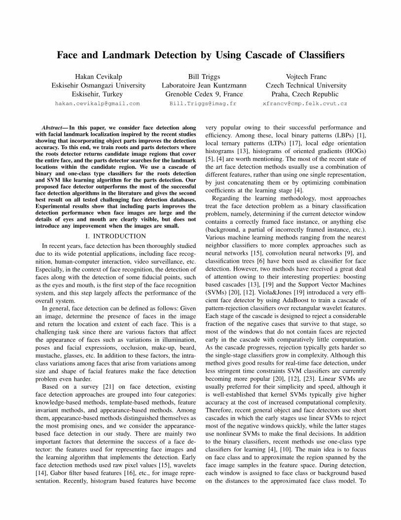
Fig. 1. Some of the tilted faces collected from real-world images.

A. Roots Detectors

Although frontal face images are considered as rigidobjects, faces coming from real-world images may be tiltedto the right or left as shown in Fig. 1. Therefore we train tworoots that are symmetric along the vertical axis. To this end,we take the mirror of each positive face image and extracttheir features. As visual features, we use LBP+HOG features.Both LBP and HOG features are extracted by using a gridof 6×6 pixel cells. For LBP, features are created by usingcircular (8,1) neighborhoods, and the resulting histogramswere normalized to sum 1. For HOG, we use 9 bins ofunsigned gradient orientation over color images as in [7].Then, resulting face visual features are clustered into twoclusters: one cluster for right-tilted faces and the other forleft-tilted faces by using the convex hull clustering algorithmdefined below.

Clustering Based on Convex Hull Approximation: We havepairs of face feature vectors extracted from symmetric faceimages, and each element of any pair must be assigned to oneof the two clusters. This is a constrained clustering problemand we use a bottom-up clustering approach for this. Wefirst select the pair where the Euclidean distance between thefeature vectors is the maximum and assign them to differentclusters. Then we iteratively assign the examples of each pairto the nearest cluster. During finding the distances from anysample to the nearest cluster, we approximate each cluster byusing the convex hull of the samples within that cluster, andfind the minimum Euclidean distance from the current sam-ple to each convex hull. In order to circumvent any problemarising from the overlapping convex hulls, we compute thedistances from samples to the reduced convex hulls createdby limiting the convex combination coefficients as in [2].The nearest convex hull distance measure is more reliablethan the nearest-mean or nearest-neighbor assignment inhigh-dimensional spaces as shown in [3]. This procedure isrepeated until all pairs of examples are assigned to clusters.Then, we refine cluster assignments by randomly selectingpairs and re-computing the distances from the samples to thenearest clusters.

1) Cascade of Classifiers: Once we split the face featuresinto two clusters, we train a root detector for each split byusing a cascade of classifiers. Our cascade has four stages.The first stage is a linear SVM classifier and it efficiently

rejects as many of the background samples while keepingalmost all face samples to the next stage. The second stageis a one-class type classifier that approximates the positivedata by a hyperplane. This stage is also computationallyvery efficient and it passes almost all face examples whilerejecting some of the background samples that passed thefirst stage. The third stage is a linear SVDD (SupportVector Data Description) classifier [18], which is based on ahypersphere model in the (non-kernelized) input space. Thisis also quite fast and it works in a complementary way withthe previous cascades by rejecting most of the false positivesthat passed the first two stages. The last stage of the cascademakes the final decision, and it uses a nonlinear (kernelized)hyperpshere model to approximate the object class. This isslower, but it operates only on a small number of positivesand difficult negatives passed the previous stages. We nowpresent each of these stages in details by omitting the well-known linear SVM classifier.

Linear Hyperplane Approximation: The second stage of thecascade approximates the face class by an hyperplane andtests the distance of a given sample feature to this hyperplane.If the distance is between some pre-defined thresholds weconsider it as a face sample and a background sampleotherwise. To this end, we find an hyperplane that fitsthe face samples best and at the same time far from thenegative samples at least by a predefined margin. Let x bethe sample’s feature vector and let w>x + b = 0 be theequation of the hyperplane. In that case, finding the bestfitting discriminative hyperplane problem can be formulatedas

arg minw,ξ≥0

1

2||w||2 + C+

∑i

(ξi + ξ∗i ) + C−∑j

ξj

s.t. w>xi + b ≤ ∆ + ξi,

w>xi + b ≥ −∆− ξ∗i ,w>xj + b ≥ ∆ + 1− ξj , i ∈ I+, j ∈ I−.

(1)

Here C+(C−) is a user defined parameter that controls theweight of the errors associated to the positive (negative)samples, I+(I−) is the set including indices of positive(negative) samples, and ∆ is a constant that can be set a valuebetween 0 and 1. By this formulation, we are constrainingpositive face samples to lie between two parallel hyperplanesw>x + b = ∆ and w>x + b = −∆. The negative sampleslie to the right of the hyperplane w>x+b = 1+∆ separatedfrom positive samples by at least margin 1/||w|| (A betterapproach would be to let negative samples lie on both sidesof the hyperplane, but this problem is not convex and hard tosolve for large scale data.) Positive slack variables, ξi, ξ∗i , ξj ,are introduced for the samples violating the constraints. Thisis a convex-quadratic programming problem that can besolved by any quadratic program solver. In high-dimensionalspaces, this formulation gives a more robust fitting comparedto the least-squares based fitting formulation described in [4].

Linear Hypersphere Approximation: The third stage of thecascade consists of a single linear SVDD classifier [18]. This

classifier uses bounding hyperspheres to approximate classes.The bounding hypersphere of a point set {xi|i = 1...n} ischaracterized by its center c and radius r. These can be foundby solving the quadratic programming problem

arg minc, r≥0, ξ≥0

(r2 + γ

∑i

ξi

)s.t. ‖xi − c‖2 ≤ r2 + ξi, i = 1, . . . , n,

(2)

or its dual

arg minα

∑i,j

αiαj 〈xi,xj〉 −∑i

αi ‖xi‖2

s.t.∑i

αi = 1, ∀i 0 ≤ αi ≤ γ,(3)

where 〈−〉 represents the (possibly kernelized) inner product.The αi are Lagrange multipliers and γ ∈ [1/n, 1] is a ceilingparameter that can be set to a value less than one to reducethe influence of outliers. This problem is convex and itsglobal optimum can be efficiently found by using a quadraticprogramming solver.

Negative samples can be used to improve the modelby forcing them to lie outside of the bounding sphere.Suppose that we have n1 face class samples enumerated byindices i, j, and n2 background samples enumerated by l,m.The most compact bounding hypersphere that includes facesamples and excludes the background samples can be foundby solving the following quadratic programming problem

arg minc, r≥0, ξ≥0

(r2 + γ1

∑i

ξi + γ2∑l

ξl

)s.t. ‖xi − c‖2 ≤ r2 + ξi, i = 1, . . . , n1

‖xl − c‖2 ≥ r2 − ξl, l = 1, . . . , n2

(4)

or its dual

arg minα

∑i,j

αi αj 〈xi,xj〉+∑l,m

αl αm 〈xl,xm〉

− 2∑l,j

αl αj 〈xl,xj〉+ (∑l

αl ‖xl‖2 −∑i

αi ‖xi‖2)

s.t.∑i

αi −∑l

αl = 1, ∀i, j 0≤αi≤γ1, 0≤αl≤γ2.

(5)This problem is also convex, and it can be efficiently

solved by using a quadratic programming solver. Given theoptimal coefficients αi, the center of the bounding spherecan be computed as

c =∑

i αi xi −∑

l αl xl . (6)

The most of the αi coefficients are zero and the samplescorresponding to the nonzero coefficients are called thesupport vectors. It turns out that the majority of the supportvectors come from the face class samples, and the number ofthe support vectors is much less than the number of supportvectors returned by an SVM algorithm. Once we computethe center of the hypersphere, the radius can be found byusing the constraints from (4).

During face detection, we find the distance from thefeature vector of each local window to the center of the hy-persphere and reject the sample as background if the distanceis greater than radius. This is implemented efficiently sinceit only requires vector subtraction and computing the norm.

Nonlinear Hypersphere Approximation: The last stage ofthe cascade includes a kernelized hyperpshere classifier thatmakes the final decisions. The hypersphere model can bekernelized by replacing the inner products with kernel evalu-ations in (5). During detection, to evaluate the distances fromincoming samples to the center of the bounding sphere, ker-nel evaluations against the support vectors are required. Thismakes kernelized SVDD classifier significantly expensivethan its linear counterpart as the number of support vectorscan be considerable. But since the kernelized hypersphereclassifier operates on a few samples that pass all previouscascades, the overall speed is still good. In practice, ker-nelized SVDD classifiers are much faster than the analogouskernelized SVMs because they have far fewer support vectorssince the support vectors come predominantly from the facetraining samples. As a result, kernel hypersphere classifier isbetter suited to use in efficient detection cascades than kernelSVM as demonstrated in [4].

B. Parts Detectors

For characterizing parts detector, we follow the proceduredescribed in [7] with small changes. In our case, a partmodel for a face with n-parts is defined by a (n + 1)-tupleP1, P2, ..., Pn, b where Pi is a model for the i-th part and bis a real-valued bias. As in [7], each part model Pi is alsodefined by a 3-tuple (fi, vi, di) where fi is a filter for thei-th part, vi is a 2-dimensional vector specifying an anchorposition for part i relative to the root position, and di isa 4-dimensional vector that specifies the coefficients of aquadratic function defining the deformation cost. The finalscore of a part detector at position li = (xi, yi) within anyimage feature space H is computed as

score(P1, ..., Pn) =

n∑i=1

f>i Φ(H,Pi)−n∑

i=1

diΦ(dxi, dyi)+b,

(7)where (dxi, dyi) gives the displacement of the i-thpart relative to its anchor position and Φ(dxi, dyi) =(dxi, dyi, dx

2i , dy

2i ) are deformation features, and Φ(H,Pi)

represents image feature for the i-th part. Concatenatingthese parameters into a single vector β, the score can bewritten as β>Φ(H, z).

We use root filter (the normal of the separating hyperplanereturned by the SVM classifier during roots detector training)as in [7] to initialize the part filters. We set the number ofparts to be 3 (two parts for the eyes and one part for themouth) and we manually place the parts into the regionswhere the eyes and mouth occur in a frontal face view asshown in Fig. 2. The part filters are initialized by interpolat-ing the root filter to twice the spatial resolution. The deforma-tion parameters are initialized to di = (0, 0, 0.05, 0.05). Byusing initial model, we extract features Φ(H, z) belonging

Fig. 2. Initialization of part filters from the root filter. We use 3 parts todetect eyes and mouth. Colored rectangles show the initial parts filters.

to the positive and negative samples and iteratively learn thenew model parameters by solving the following SVM-likequadratic optimization problem

arg minβ,ξ≥0

1

2β>β + C

∑i

ξi

s.t. β>Φ(H, zi) + b ≥ 1− ξi, ∀i ∈ I+,β>Φ(H, zi) + b ≤ −1 + ξi, ∀i ∈ I−,βk ≤ 0,∀k ∈ D,

(8)

where D is the set of indices corresponding to the quadraticdeformation terms, dx2, dy2. This is different than theclassical SVM formulation in the sense that we force thefilter coefficients corresponding to the quadratic terms tobe negative so that they will be always subtracted duringcomputation of parts scores. As in linear SVM classifier,the positive examples will be separated from the negativeexamples by a margin 2/||β||.

To solve (8) we adapted the optimized cutting plane(OCA) algorithm [8] which has been proved efficient forsolving large-scale quadratic problems emerging in the SVMtraining. The OCA algorithm incrementally constructs acutting plane model of the problem using a novel strategyto efficiently approximate the objective function around itsoptimum. The cutting plane model is used to find a searchdirection in the parameter space and a new iterate is obtainedby an exact line-search procedure. In contrast to the standardSVM training, the problem (8) contains additional constraintspreventing a subset of parameters to be positive. This modifi-cation requires slight changes to the original OCA algorithm.In particular, the new constraints must be incorporated to theexact line-search procedure and the inner quadratic solver.Our implementation of the solver can be downloaded fromhttp://cmp.felk.cvut.cz/∼xfrancv/ocas/html/index.html.

III. EXPERIMENTS

Our face detector is trained by using 21K face imagescollected from web and various face recognition databasesand 100K negative examples. We used LBP+HOG featuresas described before. We used only positive face samples tolearn linear hypersphere model (optimization problem givenin (3)) and used both negative and positive samples to learnkernelized hypersphere model (optimization problem givenin (5)). We tested our detector1 on two face detection datasetsand compared our results with those of OpenCV Viola-Jonescascade detector [19], boosted frontal face detector of Kalalet al. [11], our previous cascade detector [4] that includes asingle root detector, and part-model based detector of Zhuand Ramanan [23]. PASCAL VOC metric is used to assessthe detection performance. In this metric, detections areconsidered as true or false based on the overlap with groundtruth bounding boxes. The overlap between the boundingboxes, R returned by the classifiers, and the ground truthbox Q, is computed as area|Q∩R|

area|Q∪R| . Bounding boxes with anoverlap of 45% (we used 45% rather than 50% to compensatefor the differences between bounding box annotation choicesbetween different people and detector outputs) or greaterare considered as true positives. Then we report averageprecision (AP) for the whole Precision-Recall curve.

A. Results on Faces in the Wild Dataset

We have used 13127 images including frontal faces fromthis dataset. It should be noted that the majority of thefaces appear in the middle, and they are scaled to fit tothe same resolution. This limits its value as test set formulti-scale face detectors. In our proposed method, searchwindow size for root detectors is 36× 30, and part detectorsare applied to windows with size 72 × 60 (twice the rootdetector window size). Part-based detector of Zhu&Ramanan[23] returns only face parts and face region is estimatedas the tightest bounding box including all face parts. Thismethod works with high-resolution images where the facesare larger than 80 × 80 pixels. The images in the Facesin the Wild dataset are typically high-resolution images,where the faces in the images are around 90 × 100 pixels.Thus, part-based methods are successfully applied. The APscores are given in Table I. The best detection accuracyis obtained by part-based detector of Zhu&Ramanan [23].Our proposed method comes the second followed by the ourprevious method [4] using only one root detector (withoutparts detectors). Cascade detector of Viola&Jones [19] is theworst performing method. In general, part-based detectorsyield more successful detection accuracies for this database.

B. Results on Extended ESOGU Face Detection Database

We also tested detectors on extended ESOGU (ESkisehirOsmanGazi University) frontal face database2. The original

1Available at http://www2.ogu.edu.tr/∼mlcv/softwarecvpr2012.html2Available at http://mlcvdb.ogu.edu.tr/facedetection.html

TABLE IAVERAGE PRECISION (AREA UNDER CURVE) SCORES (%) ON THE FACES

IN THE WILD DATABASE.

Methods Average PrecisionProposed Method 94.39Viola&Jones [19] 80.23Kalal et al. [11] 87.89Cevikalp&Triggs [4] 94.12Zhu&Ramanan [23] 96.90

TABLE IIAVERAGE PRECISION (AREA UNDER CURVE) SCORES (%) ON THE

EXTENDED ESOGU FACE DETECTION DATABASE.

Methods Average PrecisionProposed Method 83.86Viola&Jones [19] 73.61Kalal et al. [11] 79.67Cevikalp&Triggs [4] 87.05Zhu&Ramanan [23] 50.55

database contained 285 higher-resolution color images in-cluding faces that appear at a wide range of image positionsand scales, and also complex backgrounds, occlusions andillumination variations. We extended the database by adding382 new images. Thus, the database now includes 667 imagesthat contains 2042 annotated frontal faces. The AP resultsof tested detectors are given in Table II, and correspondingPrecision-Recall curves are plotted in Fig. 3. The bestperforming method of Zhu&Ramanan [23] on Faces in theWild database gives the worst accuracy for this databasesince there are many faces smaller than 80 × 80 pixels inthis database. The best accuracy is achieved by our previouscascade detector [4] followed by the proposed method. Formany faces, the sizes of the images are too small to searchfor the parts, thus we upsample the face region in suchcases. But, returned parts mostly fail for upsampled low-resolution faces. The face detector of Kalal et al. [11] comesthe third best performing method. We also compared theresults to a commercial system Google Picasa3. To this end,we visually counted the number of faces returned by thepeople tagging tool of this system. We considered all returnedface images as true positives although some faces do notsatisfy PASCAL VOC overlapping criterion. We also ignoredall false positives coming from the background. In this case,the recall rate is computed as 91.52% and it is plotted inFig. 3.

C. Discussion

Our tests on challenging data sets show that the currentface detectors mostly tolerate to small rotations and illumina-tion changes, but fail to detect faces when the rotations andillumination changes are severe. They also typically cannotdetect faces smaller than 30× 30 pixels. Part-based modelswork well if the face images are large and eyes and mouthare clearly visible within the face region. If this condition is

3Available at http://picasa.google.com

Fig. 4. Some examples of the output of our cascade detector on images from the Faces in the Wild dataset (top two rows) and ESOGU face dataset(the remaining rows). Yellow rectangles show true human annotations, green rectangles show the correct detections based on PASCAL VOC criterion, andred rectangles show the false positives. Most of the faces are correctly detected, but there are a few missed detections and false positives. Part detectorstypically locate the eyes and mouth correctly if the face image region is large, but mostly fail for the small faces. Part detectors also fail to locate eyes ifthe person wears sunglasses or if the returned face region is much larger or smaller than the actual face area (e.g., the last example on the bottom right).

Fig. 3. Presicion-Recall curves for the extended ESOGU face detectiondatabase.

not met, it is better to rely only on the root detectors (for low-resolution images, simple techniques such as thresh-holdingcombined with prior information on the location of fiducialpoints can suffice to locate face fiducial points).

Results also show that there is not a significant gap be-tween the performances of the best face detectors introducedby academic community and commercial face detectors.The results are encouraging, and both face and landmarkdetectors can be integrated into face recognition systemswithout hesitation (most of the face recognition methodsproposed in the literature rely on manual face alignmentand there are only a few studies that implement a fully-automatic face recognition system). Also results on currentface recognition databases are mostly saturated, and it isnecessary to introduce more challenging face recognitiondatabases. We would also like to point out a common mistakeof face recognition methods. In most methods, the faceimages are down-sampled to small sizes such as 40 × 40pixels. However, this is a mistake in our opinion since mostof the details of the face region and parts are lost in such low-resolutions (face recognition methods work well even for thissmall sizes since the current face recognition databases aretoo easy in the sense that they are captured under controlledenvironments).

IV. CONCLUSIONWe introduced a novel face detector to find both faces

and face-parts by using the roots and parts detectors. Rootsdetectors use a cascade of binary and one-class classifiers.As a binary classifier we use linear SVM, and we use linearhyperplane and linear/kernelized hypersphere models forapproximation of face classes in one-class classifiers. Partsdetectors are traind by using a variation of SVM classifier

that enforces additional constraints on the weights of thenormal vector. Our proposed detector outperforms the mostof the succesfull face detection algorithms and gives thesecond best result on all tested challenging databases.Acknowledgments: This work was funded in part by theScientific and Technological Research Council of Turkey(TUBITAK) under Grant number EEEAG-109E279 and theYoung Scientists Award Programme (TUBA-GEBIP/2011-12) of the Turkish Academy of Sciences. The last authorwas supported by EC project FP7-ICT247525 HUMAVIPS.

REFERENCES

[1] T. Ahonen, A. Hadid, and M. Pietikainen. Face description with localbinary patterns: Application to face recognition. IEEE Transactionson PAMI, 28(12):2037–2041, 2006.

[2] K. P. Bennett and E. J. Bredensteiner. Duality and geometry in svmclassifiers. In ICML, 2000.

[3] H. Cevikalp and B. Triggs. Nearest hyperdisk methods for high-dimensional classification. In International Conference on MachineLearning, 2008.

[4] H. Cevikalp and B. Triggs. Efficient object detection using cascadesof nearest convex model classifiers. In CVPR, 2012.

[5] N. Dalal and B. Triggs. Histograms of oriented gradients for humandetection. In CVPR, 2005.

[6] M. Dantone, J. Gall, G. Fanelli, and L. V. Gool. Real-time facialfeature detection using conditional regression forests. In CVPR, 2012.

[7] P. Felzenszwalb, R. B. Girshick, D. McAllester, and D. Ramanan.Object detection with discriminatively trained part based models. IEEETransactions on PAMI, 32(9), Sept. 2010.

[8] V. Franc and S. Sonnenburg. Optimized cutting plane algorithm forlarge-scale risk minimization. Journal of Machine Learning Research,10:2157–2232, October 2009.

[9] C. Garcia and M. Delakis. A convolutional face finder: a neuralarchitecture for fast and robust face detection. IEEE Transactionson PAMI, 26(11):1408–1423, 2004.

[10] H. Jin, Q. Liu, and H. Lu. Face detection using one-class-based supportvectors. In International Conference on Automatic Face and GestureRecognition, 2004.

[11] Z. Kalal, J. Matas, and K. Mikolajczyk. Weighted sampling for large-scale boosting. In BMVC, 2008.

[12] W. Kienzle, G. Bakir, M. Franz, and B. Scholkopf. Face detection -efficient and rank deficient. In NIPS, 2005.

[13] K. Levi and Y. Weiss. Learning object detection from a small numberof examples: the importance of good features. In CVPR, 2004.

[14] C. Papageorgiou and T. Poggio. A trainable system for objectdetection. IJCV, 38:15–33, 2000.

[15] H. A. Rowley, S. Baluja, and T. Kanade. Neural network-based facedetection. IEEE Transactions on PAMI, 20:23–38, 1998.

[16] L. Shams and J. Speslstra. Learning Gabor-based features for facedetection. In World Congress in Neural Networks, 1996.

[17] X. Tan and B. Triggs. Enhanced local texture feature sets for facerecognition under difficult lighting conditions. IEEE Transactions onImage Processing, 19:1635–1650, 2010.

[18] D. M. J. Tax and R. P. W. Duin. Support vector data description.Machine Learning, 54:45–66, 2004.

[19] P. Viola and M. J. Jones. Robust real-time face detection. IJCV,57(2):137–154, 2004.

[20] C. A. Waring and X. Liu. Face detection using spectral histogramsand svms. IEEE Transactions on Systems, Man, and Cybernetcis-PartB: Cybernetics, 35:467–476, 2005.

[21] M. Yang, D. Kriegman, and N. Ahuja. Detecting faces in images: Asurvey. IEEE Transactions on PAMI, 24(1):34–58, 2002.

[22] L. Zhu, Y. Chen, A. Yulie, and W. Freeman. Latent hieararchicalstructural learning for object detection. In CVPR, 2010.

[23] X. Zhu and D. Ramanan. Face detection, pose estimation, andlandmark localization in the wild. In CVPR, 2012.