extreme value mixture modelling with simulation study and
TRANSCRIPT

Extreme Value Mixture Modelling withSimulation Study and Applications in
Finance and Insurance
By
Yang Hu
A thesis submitted in partial fulfillment of the requirementsfor the degree of Master of Science
at University of Canterbury, New ZealandJuly 2013.

Abstract
Extreme value theory has been used to develop models for describing the distribution of rareevents. The extreme value theory based models can be used for asymptotically approximatingthe behavior of the tail(s) of the distribution function. An important challenge in the applicationof such extreme value models is the choice of a threshold, beyond which point the asymptoticallyjustified extreme value models can provide good extrapolation. One approach for determiningthe threshold is to fit the all available data by an extreme value mixture model.
This thesis will review most of the existing extreme value mixture models in the literature andimplement them in a package for the statistical programming language R to make them morereadily useable by practitioners as they are not commonly available in any software. Thereare many different forms of extreme value mixture models in the literature (e.g. parametric,semi-parametric and non-parametric), which provide an automated approach for estimating thethreshold and taking into account the uncertainties with threshold selection.
However, it is not clear that how the proportion above the threshold or tail fraction should betreated as there is no consistency in the existing model derivations. This thesis will developsome new models by adaptation of the existing ones in the literature and placing them allwithin a more generalized framework for taking into account how the tail fraction is definedin the model. Various new models are proposed by extending some of the existing parametricform mixture models to have continuous density at the threshold, which has the advantage ofusing less model parameters and being more physically plausible. The generalised frameworkall the mixture models are placed within can be used for demonstrating the importance of thespecification of the tail fraction. An R package called evmix has been created to enable thesemixture models to be more easily applied and further developed. For every mixture model, thedensity, distribution, quantile, random number generation, likelihood and fitting function arepresented (Bayesian inference via MCMC is also implemented for the non-parametric extremevalue mixture models).
A simulation study investigates the performance of the various extreme value mixture mod-els under different population distributions with a representative variety of lower and uppertail behaviors. The results show that the kernel density estimator based non-parametric formmixture model is able to provide good tail estimation in general, whilst the parametric andsemi-parametric forms mixture models can give a reasonable fit if the distribution below thethreshold is correctly specified. Somewhat surprisingly, it is found that including a constraint ofcontinuity at the threshold does not substantially improve the model fit in the upper tail. Thehybrid Pareto model performs poorly as it does not include the tail fraction term. The relevantmixture models are applied to insurance and financial applications which highlight the practicalusefulness of these models.

Acknowledgments
I would like to thank my supervisors Dr Carl Scarrott and Associate Professor Marco Reale fortheir support and guidance throughout my study.
I would like to thank all the members in the Department of Mathematics and Statistics at Uni-versity of Canterbury. In particular, thanks to Steve Gourdie and Paul Brouwers for providingIT support.
Another thank you goes to all the postgraduate students in the department, who have made mytime as a student very enjoyable. Special thanks must go to James Dent for reading my draftthesis and to Chitraka Wickramarachchi for discussing statistics questions.
Finally, I would like to thank my parents for their endless support and encouragement throughmy study.
1

Contents
1 Introduction 51.1 Motivation . . . . . . . . . . . . . . . . . . . . . . . . . . . . . . . . . . . . . . . 51.2 Thesis Objectives . . . . . . . . . . . . . . . . . . . . . . . . . . . . . . . . . . . 61.3 Thesis Structure . . . . . . . . . . . . . . . . . . . . . . . . . . . . . . . . . . . . 7
2 Background 82.1 Extreme Value Theory . . . . . . . . . . . . . . . . . . . . . . . . . . . . . . . . 8
2.1.1 Extreme Value Modeling . . . . . . . . . . . . . . . . . . . . . . . . . . . 82.1.1.1 Generalized Extreme Value Distribution (GEV distribution) . . 92.1.1.2 Generalized Pareto Distribution (GPD) . . . . . . . . . . . . . 11
2.2 Threshold Choice and Common Approach . . . . . . . . . . . . . . . . . . . . . 132.2.1 Threshold Choice . . . . . . . . . . . . . . . . . . . . . . . . . . . . . . . 13
2.2.1.1 Parameter Stability Plot . . . . . . . . . . . . . . . . . . . . . . 132.2.1.2 Mean Residual Life Plot . . . . . . . . . . . . . . . . . . . . . . 142.2.1.3 Model Fit Diagnostic Plot . . . . . . . . . . . . . . . . . . . . . 14
2.2.2 Discussion and example . . . . . . . . . . . . . . . . . . . . . . . . . . . 142.3 Point Process Representation . . . . . . . . . . . . . . . . . . . . . . . . . . . . 16
2.3.1 Point Process Theory . . . . . . . . . . . . . . . . . . . . . . . . . . . . . 162.3.2 Likelihood Function . . . . . . . . . . . . . . . . . . . . . . . . . . . . . . 18
2.4 Kernel Density Estimation . . . . . . . . . . . . . . . . . . . . . . . . . . . . . . 192.4.1 Introduction . . . . . . . . . . . . . . . . . . . . . . . . . . . . . . . . . . 192.4.2 The Univariate Kernel Density Estimator . . . . . . . . . . . . . . . . . . 192.4.3 Bandwidth Selection . . . . . . . . . . . . . . . . . . . . . . . . . . . . . 202.4.4 Boundary Bias and Consistency . . . . . . . . . . . . . . . . . . . . . . . 202.4.5 Boundary Correction Estimator . . . . . . . . . . . . . . . . . . . . . . . 212.4.6 Non-Negative Boundary Correction Estimator . . . . . . . . . . . . . . . 222.4.7 Likelihood Inference for the Bandwidth . . . . . . . . . . . . . . . . . . . 23
3 Literature Review in Extremal Mixture Models 243.1 Background . . . . . . . . . . . . . . . . . . . . . . . . . . . . . . . . . . . . . . 243.2 Extremal Mixture Models . . . . . . . . . . . . . . . . . . . . . . . . . . . . . . 26
3.2.1 Behrens et al. (2004) . . . . . . . . . . . . . . . . . . . . . . . . . . . . . 263.2.2 Carreau and Bengio (2008) . . . . . . . . . . . . . . . . . . . . . . . . . . 283.2.3 Frigessi et al. (2002) . . . . . . . . . . . . . . . . . . . . . . . . . . . . . 303.2.4 Mendes and Lopes (2004) . . . . . . . . . . . . . . . . . . . . . . . . . . 313.2.5 Zhao et al. (2010) . . . . . . . . . . . . . . . . . . . . . . . . . . . . . . . 32
2

3.2.6 Tancredi et al. (2006) . . . . . . . . . . . . . . . . . . . . . . . . . . . . . 333.2.7 MacDonald et al. (2011) . . . . . . . . . . . . . . . . . . . . . . . . . . . 343.2.8 MacDonald et al. (2013) . . . . . . . . . . . . . . . . . . . . . . . . . . . 363.2.9 Nascimento et al. (2011) . . . . . . . . . . . . . . . . . . . . . . . . . . . 373.2.10 Lee et al. (2012) . . . . . . . . . . . . . . . . . . . . . . . . . . . . . . . . 38
3.3 New Model Extensions . . . . . . . . . . . . . . . . . . . . . . . . . . . . . . . . 393.3.1 Hybrid Pareto Model with Single Continuity Constraint . . . . . . . . . . 393.3.2 Normal GPD model with Single Continuity Constraint . . . . . . . . . . 40
4 User’s Guide 424.1 Introduction . . . . . . . . . . . . . . . . . . . . . . . . . . . . . . . . . . . . . . 42
4.1.1 What is the evmix package for? . . . . . . . . . . . . . . . . . . . . . . . 424.1.2 Obtaining the package/guide . . . . . . . . . . . . . . . . . . . . . . . . . 434.1.3 Citing the package/guide . . . . . . . . . . . . . . . . . . . . . . . . . . 434.1.4 Caveat . . . . . . . . . . . . . . . . . . . . . . . . . . . . . . . . . . . . . 444.1.5 Legalese . . . . . . . . . . . . . . . . . . . . . . . . . . . . . . . . . . . . 44
4.2 Generalized Pareto distribution(GPD) . . . . . . . . . . . . . . . . . . . . . . . 444.3 Parametric Mixture Models . . . . . . . . . . . . . . . . . . . . . . . . . . . . . 45
4.3.1 Gamma/Normal/Weibull/Log-Normal/Beta GPD Model . . . . . . . . . 454.3.2 Gamma/Normal/Weibull/Log-Normal/Beta GPD with Single Continuity
Constraint Mixture Model . . . . . . . . . . . . . . . . . . . . . . . . . . 484.3.3 GPD-Normal-GPD (GNG) Model . . . . . . . . . . . . . . . . . . . . . . 504.3.4 GNG with Single Continuity Constraint Model . . . . . . . . . . . . . . . 524.3.5 Dynamically Weighted Mixture Model . . . . . . . . . . . . . . . . . . . 524.3.6 Hybrid Pareto Model . . . . . . . . . . . . . . . . . . . . . . . . . . . . . 554.3.7 Hybrid Pareto with Single Continuous Constraint Model . . . . . . . . . 57
4.4 Non-Parametric Mixture Models . . . . . . . . . . . . . . . . . . . . . . . . . . . 584.4.1 Kernel GPD Model . . . . . . . . . . . . . . . . . . . . . . . . . . . . . . 594.4.2 Two Tailed Kernel GPD Model . . . . . . . . . . . . . . . . . . . . . . . 604.4.3 Boundary Corrected Kernel GPD Model . . . . . . . . . . . . . . . . . . 63
5 Simulation Study 655.1 Introduction . . . . . . . . . . . . . . . . . . . . . . . . . . . . . . . . . . . . . . 655.2 Simulation Parameters for Inference . . . . . . . . . . . . . . . . . . . . . . . . . 66
5.2.1 Initial Value For The Likelihood Inference Based Model . . . . . . . . . . 665.2.1.1 Optimization Method And Quantile Estimation . . . . . . . . . 66
5.2.2 Initial Value for the Bayesian Inference Based Model . . . . . . . . . . . 665.2.2.1 Prior Information in Bayesian Inference . . . . . . . . . . . . . 675.2.2.2 Quantile Calculation . . . . . . . . . . . . . . . . . . . . . . . . 67
5.3 A Single Tail Model With Full Support . . . . . . . . . . . . . . . . . . . . . . . 675.3.1 Parameterised Tail Fraction Approach . . . . . . . . . . . . . . . . . . . 695.3.2 Bulk Model Based Tail Fraction Approach . . . . . . . . . . . . . . . . . 70
5.4 A Single Tail Model With Bounded Positive Support . . . . . . . . . . . . . . . 715.4.1 Parameterised Tail Fraction Approach . . . . . . . . . . . . . . . . . . . 725.4.2 Bulk Model Based Tail Fraction Approach . . . . . . . . . . . . . . . . . 74
5.5 Two Tail Model With Full Support . . . . . . . . . . . . . . . . . . . . . . . . . 75
3

5.5.1 Parameterised Tail Fraction Approach . . . . . . . . . . . . . . . . . . . 755.5.2 Bulk Model Based Tail Fraction Approach . . . . . . . . . . . . . . . . . 75
5.6 Likelihood Inference For The Kernel GPD And Boundary Corrected Kernel GPDModel . . . . . . . . . . . . . . . . . . . . . . . . . . . . . . . . . . . . . . . . . 75
5.7 Main Result . . . . . . . . . . . . . . . . . . . . . . . . . . . . . . . . . . . . . . 76
6 Applications 956.1 Introduction . . . . . . . . . . . . . . . . . . . . . . . . . . . . . . . . . . . . . . 956.2 Application to Danish Fire Insurance Data . . . . . . . . . . . . . . . . . . . . . 956.3 Application to FTSE 100 Index Log Daily Return Data . . . . . . . . . . . . . . 996.4 Application to Fort Collins Precipitation Data . . . . . . . . . . . . . . . . . . . 103
7 Conclusion and Future Work 1077.1 Summary . . . . . . . . . . . . . . . . . . . . . . . . . . . . . . . . . . . . . . . 1077.2 My Contributions . . . . . . . . . . . . . . . . . . . . . . . . . . . . . . . . . . . 1087.3 Future Work . . . . . . . . . . . . . . . . . . . . . . . . . . . . . . . . . . . . . . 109
Bibliography 109
4

Chapter 1
Introduction
1.1 Motivation
Extreme value theory is used to describe the likelihood of unusual behavior or rare eventsoccurring, and has been used to develop mathematically and statistically justifiable modelswhich can be reliably extrapolated. Extremal data are inherently scarce, thus making inferencechallenging. Extreme value modeling has been widely used in financial, insurance, hydrologyor environmental applications where the risk of extreme events is of interest. A good referencebook that discusses different applications with extreme value theory is by Reiss and Thomas(2001). In this thesis, I will apply the relevant models to financial, insurance and hydrologyapplications.
It is well known that financial data often exhibit heavy (heavier than normal) tails with depen-dences, which makes the inference more challenging and problematic. However, extreme valuemodeling often assumes that the observations are independent and identically distributed (iid).One way of overcoming such issues is to use a volatility model to capture the dependence, whichleads to clustering of extreme values. The autoregressive conditional heteroskedasticity (ARCH)and generalized autoregressive conditional heteroskedasticity (GARCH) volatility model havebeen extensively used in financial applications. One of the most influential papers is by McNeiland Frey (2000). They develop the two stage approach by fitting the GARCH model at the firststage to describe the volatility clustering and then the generalised Pareto distribution(GPD)fits to the tails of the residual. Zhao et al. (2010) further extend this method at the secondstage by fitting GPDs on both lower and upper tails of the residuals, with a truncated normaldistribution for the main mode in an extreme value mixture model.
Extreme value theory also plays an important role in insurance risk management, as the insurancecompany needs to consider the potential risk of large claims (e.g. earthquake, volcanic eruptions,landslides and other possibilities). The actuary will estimate the price of the insurance products(net premium) to cover the potential insurance risk. In particular, it is of great importance forre-insurance. McNeil (1997) studies the classic Danish insurance data by applying the peaksover threshold method. Resnick (1997) acknowledges that McNeil’s work is of great importancein insurance claim application and an excellent example of adopting the extreme value model.Embrechts (1999) demonstrates that extreme value theory is a very useful tool for insurance riskmanagement.
5

In the hydrology field, flood damage can cause a lot of losses. Researchers aim to predict theprobability of the next flood event, which could be important for future plans. They often studythe flood frequency and associated flood intensity. Rossi et al. (1984) and Cooley et al. (2007)use extreme value theory models for flood frequency analysis. Katz et al. (2002) investigate theextreme events in hydrology as well. Similarly, sea-level analysis is also a very hot research topicin hydrology field. For example, Smith (1989) and Tawn (1990) apply extreme value modelingto the sea level applications.
Based on the above, extreme value modeling has attracted great interest in many differentfields. In particular, the GPD is a very popular extreme value model, which can give a goodmodel for the upper tail providing reliable extrapolation for quantiles beyond a sufficiently highthreshold. An important challenge in application of such extreme value models is the choice ofthreshold, beyond which the data can be considered as extreme data or more formally wherethe asymptotically justified extreme value models will provide an adequate approximation tothe tail of the distribution. Various approaches have been developed to aid the selection of thethreshold, all with their own advantages and disadvantages. Recently, there has been increasinginterests in extreme value mixture models, which not only consider the threshold estimation butalso the quantification of the uncertainties that result from the threshold choice.
1.2 Thesis Objectives
The main purpose of the thesis is to implement the existing extreme value mixture models in thestatistical package R and create a library to make these more readily available for practitioners touse. This library will include both likelihood and computational Bayesian inference approacheswhere appropriate. A detailed simulation study is carried out which aims to compare differentextreme value mixture model properties to provide some concrete advice about the performanceof each mixture model and guidance on how their formulation influences their performance.
There is no generalized framework for defining these extreme value mixture models. In particular,there is no consistency in terms of how the proportion of the population φu above the threshold isdefined in the model and subsequently estimated. The proportion in the upper tail is sometimesreferred to as the tail fraction, which treated as a parameter the MLE is the sample proportion.However, it is common when defining extreme value mixture models to allow the tail fraction φuto be inferred by the proportion of the bulk model. The approach of treating the tail fractionas a parameter estimated using the MLE is consistent with traditional applications of the GPD.However, the definition using the bulk model is commonplace and has no formal justificationand apart from convenience. This thesis derives a general framework for the extreme valuemixture models which permits the tail fraction, φu to be specified in either of these forms, andwill explore which approach performs well in general.
The parametric form of mixture models provide the simplest form of extreme value mixturemodels (e.g. Frigessi et al. (2002), Behrens et al. (2004) and Zhao et al. (2010)). These modelstypically treat threshold as a parameter to be estimated. The main concern is whether they canprovide sufficient flexibility if they are mis-specified.
Continuity at the threshold is another common issue with some of these mixture models, asmost of them do not require the density function to be continuous at the threshold. Carreau and
6

Bengio (2008) develop the hybrid Pareto model by combining a normal and a GPD distributionand set two continuity constraints at the threshold (i.e. continuity in zeroth and first derivative).They claim that this model works well for heavy tailed and asymmetric distribution. This thesiswill evaluate that claim, and explore whether this mixture model can perform well or not inshort or exponential tail distribution. The simulation study will also explore whether the extracontinuity constraint at the threshold would improve the model performance.
1.3 Thesis Structure
Chapter 2 summaries the key background material on relevant statistical topics including ex-treme value theory, mixture models and kernel density estimator.
Chapter 3 reviews the existing extreme value mixture models approaches, with some referencesto alternative approaches in the literature. All of these existing models are placed within mynew generalised framework, with a consistent notation used throughout. Some new models Ihave created by extensions from the original mixture models are also presented.
Chapter 4 demonstrates the usage of the R library I have developed implementing these mixturemodels. A very detailed simulation study is carried out in Chapter 5. The different extremalmixture models are divided into three groups in evaluating their performance based on thesupport of the distribution and whether a single tail or both tails are described. The simulationstudy will consider the following questions:
• How does each model perform in general for tail estimation? Is there a “best” mixturemodel, or “best type” of mixture model? Are there any which can perform poorly incertain situations?
• Is it better to specify the tail fraction in terms of a parameter to be estimated, or to usethe bulk model tail fraction?
• Is it better to include a constraint that the density be continuous at the threshold?
In the chapter 6, all the relevant models are applied to the classic Danish insurance data, FTSE100 index log daily return data and Fort Collins precipitation data.
7

Chapter 2
Background
2.1 Extreme Value Theory
This chapter will review the classic probabilistic extreme value theory and the classical modelsused for describing extreme events. Followed by an overview of kernel density estimation tosupport the presentation in the rest thesis.
2.1.1 Extreme Value Modeling
Classical extreme value theory is used to develop stochastic models towards solve real life prob-lems related to unusual events. Classical theoretical results are concerned with the stochasticbehavior of some maximum (minimum) of a sequence of random variables which are assumed tobe independently and identically distributed.
Coles (2001) explains that let X1, ..., Xn be a sequence of independent random variable withpopulation distribution function F and Mn represents the maxima or minima of the processover the block size n. The distribution of Mn can be derived by:
Pr {Mn ≤ x} = Pr {X1 ≤ x, . . . , Xn ≤ x} = Pr {X1 ≤ x} × · · · × Pr {Xn ≤ x} = {F (x)}n .
If the population distribution is known, the distribution of Mn can be determined exactly.However, in the more usual case of unknown population distributions, the distribution of Mn
can be approximated by modeling F n through asymptotic theory of Mn. As n → ∞, thedistribution of Mn will degenerate to a point mass at the upper end point of F . For mostpopulation distributions this degeneracy problem can be eliminated by allowing some linearrenormalization of the Mn, similar to that used in the Central Limit Theorem. Consider a linearrenormalization:
M∗n =
Mn − bnan
,
for sequences of constants an > 0 and bn. After choosing suitable an and bn, the distribution ofMn may be stabilized and which lead to extremal types theorem.
Extremal Types Theorem. If there exists sequences of constants {an > 0} and {bn}, as n→∞, such that
Pr {(Mn − bn)/an ≤ x} → G(x)
8

where G is a non-degenerate distribution function, then G belongs to one of the following families:
I : Gumbel : G(x) = exp
{− exp
[−(x− µσ
)]}−∞ < x <∞; (2.1)
II : Frechet : G(x) =
0, x ≤ µ;
exp
{−(x− µσ
)}, x > µ;
(2.2)
III : Weibull : G(x) =
exp
{−
[−(x− µσ
)−ξ]}, x ≤ µ;
1, x > µ;
(2.3)
for parameters σ > 0, µ ∈ R.
The proof of this theorem can be found in Leadbetter et al. (1983). The extremal types theoremsuggests that if Mn can be stabilized with choosing suitable an and bn, then the limit distributionM∗
n will be one of the three extreme value distributions. No matter what the population distri-bution of Mn is, if a non-degenerate limit can be obtained by linear renormalisation, then thesethree different extreme value distributions which have distinct behaviors are the only possiblelimit distribution of M∗
n. But there is no guarantee of a non-degenerate distribution.
For an unknown population distribution it is inappropriate to adopt one type of limiting distri-bution and ignore any uncertainties associated with family distribution. A better approach isto adopt a universal extreme value distribution which encompasses all three types as a specialcase.
2.1.1.1 Generalized Extreme Value Distribution (GEV distribution)
von Mises (1954) and Jenkinson (1955) proposed a way of unifying the three different types of ex-treme value distributions, which lead to the generalized extreme value distribution GEV(µ, σ, ξ).
Theorem 1. If there exists sequences of constants {an > 0} and {bn}, as n→∞, such that
Pr {(Mn − bn)/an ≤ x} → G(x)
where G is a non-degenerate distribution function,then G is a member of the GEV family:
G(x) = exp
{−[1 + ξ
(x− µσ
)]−1/ξ
+
}
defined on{x : 1 + ξ(x−µ
σ) > 0
}, where σ >0, µ ∈ R and ξ ∈ R.
Now µ is the location parameter, σ is the scale parameter and ξ is the shape parameter. TheGEV distribution simplifies the three different types of extreme value distributions to one family.The GEV distribution is used as an asymptotic approximation for modeling the maxima of thefinite sequences.
9

The GEV distribution provides us a way of modeling the extremes of block maxima (or minima).If the iid observations x1, ..., xi are divided into m blocks of size n, where n is large enough,then we can generate a series of sample maxima Mn,1,. . . ,Mn,m for which their distributioncan be approximated by the asymptotically motivated GEV distribution. The block size is ofimportance in GEV model. If the block size is too small, this can lead to a poor asymptoticapproximation.
The distribution function of GEV(µ, σ, ξ) is given by:
F (x|µ, σ, ξ) =
exp
{−[1 + ξ
(x− µσ
)]−1/ξ
+
}ξ 6= 0,
exp
[− exp
(−x− µ
σ
)]ξ = 0.
Figure 2.1: Examples of the density and corresponding distribution function for the GEV dis-tribution with µ = 0, σ = 0.7, and varying ξ with (0, -0.5, 0.5)
From Figure 2.1, the example demonstrates how the shape parameter affects the tail behaviorby keeping the location and scale parameters the same. If ξ = 0, the GEV distribution belongsto Gumbel distribution and it decays exponentially. If ξ < 0, the GEV belongs to the negativeWeibull distribution with a finite short upper endpoint. Otherwise, the GEV distribution belongsto the Frechet distribution, which has a heavy tail behavior.
The inverse of GEV distribution function represents the quantile function. Let F (zp) = 1 − p,where p is the upper tail probability.
zp =
u− σ
ξ
{1− [− log(1− p)]−ξ
}ξ 6= 0,
u− σ log [− log(1− p)] ξ = 0.
10

zp is referred to return level with return period of 1/p. In general, zp is exceeded on averageevery 1/p period of time. Equivalently, the average time for a very rare event to exceed the zpis every 1/p period of time. The return level is often interpreted as the expected waiting timeuntil another exceedance event.
2.1.1.2 Generalized Pareto Distribution (GPD)
The block maxima based the GEV distribution is inefficient as it is wasteful of data when thecomplete dataset (or at least all extreme values) are available. One way of overcoming thesedifficulties is to model all the data above some sufficiently high thresholds. Such a model iscommonly referred as the peaks over threshold or threshold excess model. The advantage of thethreshold excess model is that it can make use of the all the “extreme” data. Under certainconditions, Coles (2001) explains that let X1, . . . , Xn be a sequence of iid random variables,the excess X − u over a suitable u can be approximated by the generalized Pareto distributionG(x|u, σu, ξ).
The distribution function of GPD is given by:
G(x|u, σu, ξ) =
1−
[1 + ξ
(x− uσu
)]−1/ξ
+
ξ 6= 0,
1− exp
[−(x− uσu
)]+
ξ = 0.
where x > u, σu > 0,[1 + ξ
(x−uσu
)]> 0 and σu reminds us the dependence between scale
parameter σu and threshold u. The dependence of the GPD scale σu on the threshold is madeexplicit by the subscript u, which is also retained in the functions in the R package described inChapter 4.
The shape parameter ξ is of importance in determining the tail distribution of the GPD:
• ξ < 0: short tail with finite upper end point of u− σuξ
;
• ξ = 0 : exponential tail; and
• ξ > 0: heavy tail.
GPD is defined conditionally on being above threshold u. The unconditional survival probabilityis defined as:
Pr(X > x) = Pr(X > u) ∗ Pr(X > x|X > u)
= Pr(X > u) ∗ [1− Pr(X < x|X > u)]
= φu ∗ [1−G(x|u, σu, ξ)],
where φu = Pr(X > u) is the probability of being above the threshold. The value of φu is an-other parameter required when using the GPD. It is an implicit parameter which is oftenforgotten about.
11

It would be worth showing how GEV and GPD models are related with each other. Let Yfollows GEV distribution over a high threshold u and y is the excess (x− u).
Pr{Y > u+ y|Y > u} =1− Pr(Y < y + u)
1− Pr(Y < u)
≈ [1 + ξ(u+ y − µ)/σ]−1/ξ
[1 + ξ(u− µ)/σ]−1/ξ
=
[1 +
ξ(u+ y − µ)/σ
1 + ξ(u− µ)/σ
]−1/ξ
=
[1 +
ξy
σu
]−1/ξ
,
where σu = σ + ξ(u − µ). This derivation makes the dependence of the GPD scale σu andthreshold u very clear. The GPD shape parameter is the same as the GEV shape parameter.
Maximum Likelihood Estimation of GPD
Let x1, ..., xn be a sequence of observations of independent random variables which are theexceedances above a threshold u. The log-likelihood function is derived from taking logarithmof the joint density function. Let nu be the number of observations above the threshold u.
logL(σu, ξ|X) = −nu log σu − (1 + 1/ξ)nu∑i=1
log
[1 + ξ
(xi − uσu
)],
with
[1 + ξ
(xi − uσu
)]> 0 and ξ 6= 0. The constraint
[1 + ξ
(xi − uσu
)]implies x < µ− σu/ξ.
When ξ = 0, the log-likelihood function can be derived in similar way:
logL(σu|X) = −nu log σu −nu∑i=1
(xi − uσu
)with ξ = 0.
Regularity condition
There are certain regularity conditions for the maximum likelihood estimators to exhibit theusual asymptotic properties. It is worthwhile to notice that maximum likelihood estimatorsare not always valid and the regularity conditions do not always exist. The invalid regularityconditions are caused by upper endpoint of GEV distribution being dependent on the parameterswhere the endpoints are parameter value of µ− σu/ξ when ξ < 0.
Smith (1985) has outlined the following result:
• ξ > −0.5, maximum likelihood estimators have usual asymptotic properties;
• −1 < ξ < −0.5, maximum likelihood estimators generally exist, but do not have usualasymptotic properties;
12

• ξ < −1, maximum likelihood estimators generally do not exist.
In general, the GPD distribution has a very short bounded upper tail behavior if ξ ≤ −0.5, sorarely comes up in applications.
2.2 Threshold Choice and Common Approach
This section will demonstrate the difficulty in choosing the threshold through the commondiagnostic plots used in practice.
2.2.1 Threshold Choice
Threshold selection is still an area of ongoing research in the literature which can be of thecritical importance. Coles (2001) states that the selection of the threshold process always is atrade-off between the bias and variance. If the threshold is too low the asymptotic argumentsunderlying the derivation of the GPD model are violated. By contrast, too high a thresholdwill generates fewer excesses (x− u) to estimate the shape and scale parameter leading to highvariance. Thus threshold selection requires considering whether the limiting model provides asufficiently good approximation versus the variance of the parameter estimate.
In the traditional extreme value modeling approaches, the threshold is chosen and fixed beforethe model is fitted which is commonly regarded as the fixed threshold approach. Various di-agnostics plots to evaluate the model fit are commonly used for choosing the threshold. Coles(2001) outlined three diagnostics for the choice of threshold including the mean residual life plot,parameter stability plot and more general model fit diagnostics plots.
2.2.1.1 Parameter Stability Plot
Another plot that can be used for assessing the model fit to judge the threshold is usually referredas the parameter stability plot.
If the excesses over a high threshold u follow a GPD with ξ and σu, for any higher thresholdv > u, the excesses still follow a GPD with ξ but with scale parameter of :
σv = σu + ξ(v − u).
By re-parametrise the scale parameter σv:
σ∗ = σv − ξv.
The σ∗ now no longer depends on v, given that u is a reasonably high threshold. This plot fitsGPD over a certain values of thresholds against the shape and scale parameter. The thresholdu should be chosen where the shape and modified scale parameter remain constant after takingthe sampling variability into account. Once a suitable threshold is reached, the excess over thisthreshold follows GPD.
13
2.2.1.2 Mean Residual Life Plot
If the excess X − u are approximated by a GPD, for a suitable u, the mean excess is:
E(X − u|X > u) =σu
1− ξfor ξ < 1
For any higher threshold v > u, the mean excess is defined as:
E(X − v|X > v) =σv
1− ξ=σu + ξ(v − u)
1− ξfor ξ < 1
It shows that the mean excesses E(X − u|X > u) is a linear function of u, once a suitable highthreshold u has been reached.
The sample mean residual life plot points, drawn using the(u,
1
nu
nu∑i=1
(x(i) − u)
)
where x(i) is the observation above the u and nu is the number of observation above the u.For a sufficiently high threshold u, all the excesses v > u in the mean residual life plot changeslinearly with u. This property could potentially provide a way of choosing the the threshold.Once the sampling variability is included, the threshold should be chosen where the relationshipfor mean excess of all higher thresholds is linear. Coles (2001) concluded that interpretation ofsuch plot is not an easy task.
Both the mean residual life and parameter stability plot are popular choices for graphicallychoose for the threshold.
2.2.1.3 Model Fit Diagnostic Plot
Various standard statistical model diagnostic plots such as probability plot, quantile plot, returnlevel plot and empirical versus fitted density comparison plot can be used for checking the modelfit and the suitability of the threshold choice. These checks based on a chosen threshold, so theyare post-calculation diagnostic plots. These plots provide an alternative way of assessing themodel performance.
2.2.2 Discussion and example
A possible disadvantage with these diagnostics plots is that the threshold chosen from inspect-ing the graph could suffer from substantial subjectivity expertise. The drawback with theseapproaches would mean that some different thresholds can be suggested by different practition-ers using the same diagnostics from their point of views. The following example will demonstratethat graphically inspecting data could result in substantial differences in such subjective thresh-old selection.
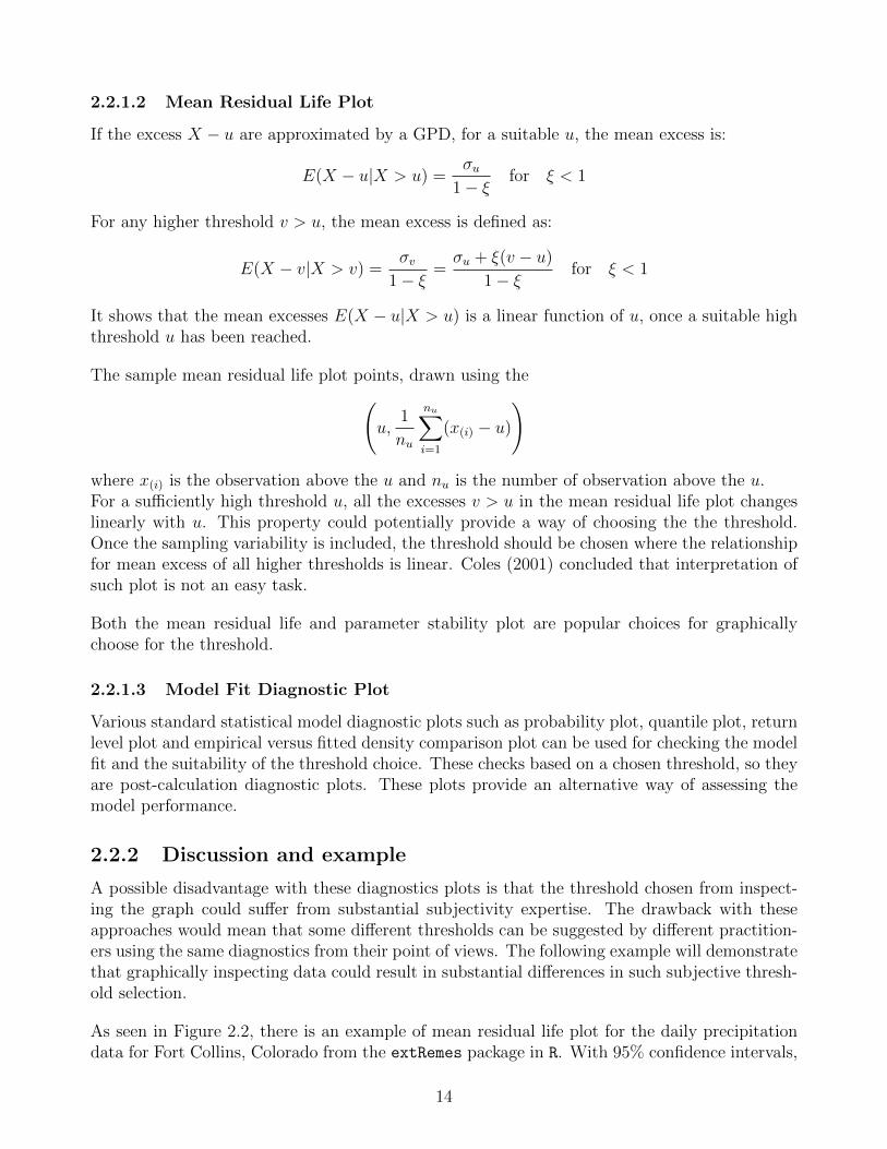
As seen in Figure 2.2, there is an example of mean residual life plot for the daily precipitationdata for Fort Collins, Colorado from the extRemes package in R. With 95% confidence intervals,
14

Figure 2.2: The mean residual life plot for Fort Collins precipitation data.
the ideal threshold u is the one where the mean excess above the threshold u is linear afterconsidering the sample variability. In order to show the problematic diagnostics for the thresholdselection, the non-stationarity and dependence of the series will be ignored. There are severalpossible choices for the thresholds. Katz et al. (2002) suggested the threshold u to be 0.395.When threshold u is 0.395, it results in a heavy tail behavior (ξ = 0.21) while the thresholdcould lead to exponential tail behavior when the threshold u is equal 1.2 (ξ = 0.003). Anotherpossible choice for u is 0.85, which exhibits a heavy tail with the shape of ξ = 0.134. From theplot, all three thresholds exhibit different tail behavior as the shape parameter varies a lot.
Figure 2.3 is the parameter stability plot for the Fort Collins daily precipitation data. Whenthe thresholds are 0.395, 0.85 and 1.2, the modified scale parameter(σ∗ in Section 2.2.1.1) seemsreach a plateau. However, if the shape parameter is taken into account, it is difficult to tellwhich the lower threshold choice is. The parameter stability plot cannot provide a consistentconclusion once the sample variability of both parameters and the negative dependence betweenthe modified scale and shape parameter are taken into account. Scarrott and MacDonald (2012)used this data to demonstrate the above threshold selection issue in detail.
These examples have shown that the diagnostics plots could result in subjective judgement.The threshold choice procedure needs a more objective approach. Not only does the traditionalthreshold selection approach face substantial subjectivity in threshold choice, but also it lacksthe considerations of uncertainty of the threshold choice in the subsequent inferences. Once thethreshold is chosen, the variability or uncertainty of the threshold will not be taken into account.Pre-fixed the threshold is at least not ideal in most cases unless there is a valid reason for doingthat. In this case, threshold is always constrained by physical objectives.
15

Figure 2.3: The parameter threshold stability plot for Fort Collins precipitation data.
2.3 Point Process Representation
The theory of point process in the extreme value literature can be dated back to Pickands(1971). Pickands (1971) presented a way of describing the classic block maximum and GPDbased extreme value model through point processes point view. The mathematical theory be-hind the point process model can be found by Leadbetter et al. (1983), Resnick (1987) andEmbrechts et al. (1997). Leadbetter et al. (1983) provided the comprehensive coverage of theclassic extreme value theory including theoretical argument for the point process properties.Resnick (1987) presented the mathematically fundamental and detailed explanation of the pointprocess characterization especially the Poisson process for the extreme value theory based onindependent and identically distributed random variables.
Coles (2001) interpreted that the point process characterization can be used to measure theprobability of a given event occurring during a particular time period or the expected time for thenext event occurring. The point process representation unifies the classic extreme value modelslike the GEV and GPD into one model. It is popular to adopt the point process representationfor GPD to solve the problem of the dependence between the scale parameter and threshold.
2.3.1 Point Process Theory
A point process describes the distribution of random points within a space. Coles (2001) explains,the most popular way of characterizing the point process is to define a set of positive integer,N(A), for each subset A ⊂ A. The set of A could be multi-dimensional, A ⊂ Rk. N(A) simplymeasures the number of points in the subset A. The characteristics of the point process N isdetermined by the distribution of every N(A) in the A.
16

The expected number of points in a set A is referred to as the intensity measure Λ(A),
Λ(A) = E(N(A)).
The intensity measure Λ has a density function λ, which is referred to as the intensity function,
λ(A; θ) =
∫A
λ(Xi; θ) dx.
A Poisson process on an Euclidean space is a point process N with intensity measure Λ whichsatisfies with the following conditions.
1 For any set of A ⊂ A, N(A) is Poisson random variable with mean Λ(A).
2 For all disjoint set A1, . . . , An, N(A1), . . . , N(An) are independent.
In other words, the number of points has a Poisson distribution and the number of points fallingin different subset are independent. One of the inherent property of a Poisson process is thatthe points occur independently of each other. If the intensity function of a Poisson process λ isconstant, then the corresponding Poisson process is referred to as a homogenous Poisson process.
Let X1, . . . , Xn be a series of independent and identically distributed random variables withcommon distribution function F, and let
Pn =
{(i
n+ 1,Xi − bnan
); i = 1, . . . , n
}Coles (2001) explains that the first ordinate is to restrict to map the time axis to (0,1) andthe second ordinate with the nonnormalizing constant an and bn is to stabilize the behaviorof Xi when n → ∞. It is known that such distribution of Pn can converge in the limit to atwo-dimensional non-homogeneous Poisson point process. For a sufficiently high threshold, thedistribution of the two-dimensional point process Pn is approximated in the limit by a non-homogeneous Poisson point process over the set A of (0, 1]× [u,∞).
The intensity measure on the subregion B = [t1, t2] × (u,∞) for the non-homogeneous Poissonpoint process is given by:
Λ(B) =
(t1 − t2)
[1 + ξ
(x− µσ
)]−1/ξ
+
ξ 6= 0
(t1 − t2) exp
{−(x− µσ
)}+
ξ = 0
The corresponding intensity function is then given by:
λ(x) =
1
σ
[1 +
ξ
σ(x− u)
]−1/ξ−1
ξ 6= 0
1
σexp
[−(x− uσ
)]ξ = 0
17

It is common to include the scaling constant variable nb which is the number of years of obser-vation to the intensity function. By doing this, the estimated (µ, σ, ξ) refers to GEV parametersfor the number of years maxima estimate. The intensity measure can be therefore given by:
Λ(B) =
(t1 − t2)nb
[1 + ξ
(x− µσ
)]−1/ξ
+
ξ 6= 0
(t1 − t2)nb exp
{−(x− µσ
)}+
ξ = 0
It is not difficult to show that GPD can be derived from the point process representation.
Pr
{(Xi − bn)
an> x
∣∣∣(Xi − bn)
an> u
}=
[1 + ξ(x−µ
σ)
1 + ξ(u−µσ
)
]−1/ξ
=
[1 +
ξ(x− u)
σu
]−1/ξ
2.3.2 Likelihood Function
The points of a Poisson process in a set A, N(A), are independent and identically distributed
with a density of λ(Xi;θ)Λ(A;θ)
. Suppose the point process Pn with the intensity measure Λ(A; θ) is on
the space of A = (0, 1]× [u,∞). For the points, x1, . . . , xnu within the space of A, the likelihoodcan be derived from:
lpp(θ, x) = exp {−Λ(A; θ)} Λ(A; θ)nu
nu!
nu∏i=1
λ(Xi; θ)
Λ(A; θ),
lpp(θ, x) ∝ exp {−Λ(A; θ)}nu∏i=1
λ(Xi; θ),
where Λ(A; θ) =∫Aλ(Xi; θ) dx.
The general from of Poisson process likelihood can be derived as:
l(u, µ, σ, ξ|x) ∝
exp
{−nb
[1 + ξ
(u− µσ
)]−1/ξ}
nu∏i=1
1
σ
[1 + ξ
(xi − µσ
)]−1/ξ−1
ξ 6= 0,
exp
[−nb exp
(u− µσ
)] nu∏i=1
1
σexp
[−(x− uσ
)]ξ = 0.
Similarly with the peaks over threshold method, the estimate obtained from the point processlikelihood are based on the data that are greater than the threshold.
18

2.4 Kernel Density Estimation
2.4.1 Introduction
Nonparametric density estimation plays an important role in analyzing data. Unlike parametricmodels, nonparametric estimation technique can be used for effectively describing the complexdata structure such as bi-modality or multi-modality without making prior assumptions aboutthat they exist and the form they take. Nonparametric density estimation doesn’t assume aspecific functional form for the population distribution, only that it is sufficiently smooth, whichprovides more flexibility in estimating the density of the underlying dataset. The subject ofnonparametric density estimation was brought to prominence by Rosenblatt (1956). One of themost popular nonparametric techniques is kernel density estimation. There has been intensivediscussion about kernel density estimation in the literature, for example Rosenblatt (1956),Parzen (1962), Watson and Leadbetter (1963) and Resnick (1987). A classic text book on thetopic is Wand and Jones (1995).
2.4.2 The Univariate Kernel Density Estimator
The traditional kernel density estimator is defined as:
f(x; x, h) =1
nh
n∑i=1
K
(x− xih
),
where K(.) is the kernel function usually defined to be a symmetric and unimodal probabilitydensity function and h is the bandwidth parameter. The kernel function usually meets thefollowing conditions: K(x) ≥ 0 and
∫K(x) dx = 1. Another formula for the kernel estimator
can be obtained by including scale kernel Kh(y) = h−1K(y/h)
f(x; x, h) = n−1
n∑i=1
Kh (x− xi)
Wand and Jones (1995) interpret that the value of the kernel estimate at the point x is simplythe average of the n kernel ordinates at that point. Various kernel functions have been proposedin the literature such as uniform, biweight, normal and other functions. The choice of the kernelfunction is not limited to some probability density functions. In this case, the resulting densityestimate will not be a density any more but can be renormalized to be a density. The normalprobability density function is a popular choice for the kernel. When the normal distribution issuggested to be the kernel function, the bandwidth h will play the role of the standard deviationin the normal distribution which controls the spread of the kernel.
Wand and Jones (1995) pointed out that the choice of the kernel function is less critical than thechoice of the bandwidth. There is always a trade-off between the bias of the resulting estimatorand corresponding variance. If the bandwidth is too low, the estimate is very spiky and thusincreasing the variance in the estimate. On the other hand, if the bandwidth is too high, thekernel estimation is too smooth leading to bias and it fails to provide adequate estimation forthe true structure of the underlying density. Thus a large bandwidth could lead to a high biasbut low variance of the estimator.
19

2.4.3 Bandwidth Selection
There are several common approaches of choosing bandwidth h in the literature. Silverman(1986) looks at varies method to choose the bandwidth parameter. A simple and natural wayof choosing the smoothing parameter is to plot several possible parameter value and choosethe best fit to the underlying the density. The process of examining the a range of possiblesmoothing parameter candidates can be inefficient, time-consuming and subjective. Anothermethod of selecting the bandwidth is to minimize some error criteria such as the mean squarederror(MSE), mean integrated squared error (MISE), mean integrated absolute error(MIAE) andother criteria. The detail of bandwidth selection is beyond the scope of this thesis. Simplerules of thumb for selecting the bandwidth are based on various measures of performance, forexample by minimizing asymptotic mean integrated squared error (AMISE). When the normaldistribution has been used as the kernel function, the optimal choice of bandwidth in terms ofminimising the AMISE, for a normal population is given by Silverman (1986):
h =
(4σ5
3n
)1/5
,
where σ is the sample standard deviation and n is the sample size.
2.4.4 Boundary Bias and Consistency
One inherent drawback of the kernel density estimator is that it has no prior knowledge aboutwhere the boundary should be. It is better to use kernel density estimator to fit some unboundeddensities. When kernel density estimator fits to the bounded density, it doesn’t achieve the samelevel of accuracy at the boundary compared to the bounded density. Jones (1993) finds thatkernel density estimator causes more bias at the boundary than the interior point. Kernel densityestimation simply assigns the probability mass outside the support and so it suffers from biasat or near the boundary.
Let K be a symmetric kernel function with support [-1,1] and the bandwidth is denoted by has usual. Suppose x = ph, p is a function of x. For any x ≥ h, or p ≥ 1, there is no overspill ofthe contributions to the boundary. For an interior point, or any x ≥ h, if the first and secondderivatives of f are continuous, the usual mean and variance can be derived:
E{f(x)
}' f(x) +
1
2h2a2(p)f ′′(x).
At or near the boundary, for any x < h,or p < 1, the usual mean and variance can be derived:
E{f(x)
}' a0(p)f(x)− ha1(p)f ′(x) +
1
2h2a2(p)f ′′(x),
V{f(x)
}' (nh)−1b(p)f(x),
where
al(p) =
∫ min{p,1}
−1
ulK(u) du and b(p) =
∫ min{p,1}
−1
K2(u) du.
20
The coefficient of the first term in the mean of the f(x) is a0(p), which can be interpreted asthe probability mass outside the boundary. Thus kernel density estimation is not a consistentestimator at the boundary. If the coefficient of the first term in the mean of the f(x) is one, thenthe estimator is regarded as a consistent estimator. Jones (1993) points out that the boundarypoint has the bias of the order O(h) while the interior point has the bias of the order O(h2).
Consequently, the kernel density estimator is more biased at or near the boundary comparedwith interior point. A boundary corrected approach is needed to achieve O(h2) bias everywhere.Jones (1993) presented two popular ways of achieving reduced bias at the boundary. The firstapproach is to use a local re-normalization technique to make the estimator become consistentat the boundary. By dividing f(x) by a0(p), the resulting estimator fN(x) is defined as:
fN(x) = f(x)/a0(p),
where a0(p) =∫ min{p,1}−1
K(u) du. The resulting estimator successfully captures that the kernel
probability mass within the boundary. fN(x) has become a consistent estimator. This localre-normalization technique (fN(x)) still gives and o(h) bias at the boundary. Another way ofreducing the bias is to reflect the data at the boundary, with the estimator given by:
fR(x) = f(x) + f(−x)
It is proven that fR(x) becomes a consistent estimator but it doesn’t achieve O(h2) bias at theboundary. Through the theoretical comparison, both approaches can overcome the consistencyissues. In general, the refection approach outperforms the re-normalization approach as therefection approach suffers a smaller bias compared with the re-normalization approach. One ofthe fundamental issues with these two estimators is that they all still suffer from the boundarybias with an order of O(h).
2.4.5 Boundary Correction Estimator
Jones (1993) suggested a generalized jackknifing idea to obtain the O(h2) bias either in theinterior or the boundary. Let K be a general kernel function with the support of [−SK , SK ].The idea is to take a linear combination of K with some other function L which is closely relatedwith function K. The corresponding kernel will have the following properties:
1. ao(p) =∫ min{p,Sk}−1
K(u) du = 1
2. a1(p) =∫ min{p,Sk}−1
uK(u) du = 0
where p is a function of x, p = xh. The first property is to make kernel mass within the boundary
and the second property is to make the first moment of each kernel center about the data point.Let L be a kernel function with support[−SL, SL]. The corresponding kernel density estimatoris defined as:
f(x) =1
n
n∑i=1
Lh (x− xi)
Like the standard kernel estimator, another formula for f(x) can be obtained as Lh(x − xi) =h−1L((x− xi)/h). By dividing c0(p), f(x) can be re-normalized as usual,
21

f(x) = f(x)/c0(p) where cl(p) =
∫ min{p,SL}
−SL
ulL(u) du.
Generalized jackknifing method undertakes such linear combination,
f(x) ≡ αxfN(x) + βxf(x).
The following linear combination is able to allow O(h2) bias either interior or boundary point,provided that c1(p)a0(p) 6= a1(p)c0(p),
αx = c1(p)a0(p)/ {c1(p)a0(p)− a1(p)c0(p)} ,βx = −a1(p)c0(p)/ {c1(p)a0(p)− a1(p)c0(p)} .
It should be noticed that such boundary corrected kernel density estimator doesn’t automaticallyintegrate to unity, which requires further re-normalizing the estimator. A popular choice for L(.)is to set L(x) = xK(x). There is a linear relationship between the L(.) and K(.). Such choice re-sults in a simple boundary corrected kernel (lx+mxx)K(x),where lx = a2(p)/ {a2(p)a0(p)− a2
1(p)}and mx = −a1(p)/ {a2(p)a0(p)− a2
1(p)}. Even though there are various boundary corrected es-timators using generalized jackknifing technique, there are little differences in the performance.Jones (1993) suggests the linear boundary corrected estimator is a good choice.
The associated boundary corrected kernel density estimator is therefore defined as:
f(x; x, h) =1
nh
n∑i=1
KL
(x− xih
),
where KL is the kernel function,
KL(x) =(a2(p)− a1(p)x)K(x)
a2(p)a0(p)− a21(p)
.
2.4.6 Non-Negative Boundary Correction Estimator
As mentioned earlier, there are several different choices for L(.) kernel, which will lead to differentboundary corrected kernel estimators. The major drawback with these generalized jackknifingestimators is the propensity to take the negative values at the boundary. Jones and Foster(1996) propose a simple non-negative boundary correction estimator, which is a combinationof boundary corrected estimator and scaled standard kernel density estimator. The resultingestimator is defined as:
fBC(x; x, hBC) ≡ f(x; x, hBC)exp
{f(x; x, hBC)
f(x; x, hBC)− 1
}.
This is a combination of boundary corrected estimator f(x; x, hBC) and scaled standard kerneldensity estimator,
f(x; x, hBC) =f(x; x, h)
a0(p).
Jones and Foster (1996) provide mathematical and theoretical justification of this estimator.They have shown that this estimator achieves the desirable property of obtaining the sameorder of bias between the interior point and near the boundary.
22

2.4.7 Likelihood Inference for the Bandwidth
The likelihood inference for kernel bandwidth was proposed by Habbema et al. (1974) and Duin(1976). The likelihood degenerates at zero bandwidth, leading to point mass at each uniquedatapoint. To avoid this degeneracy issue, they propose a cross-validation likelihood
L(λ|X) =n∏i=1
1
(n− 1)
n∑j=1j 6=i
Kλ(xi − xj)
This cross-validation likelihood is used in the Bayesian inference MacDonald et al. (2011) andMacDonald et al. (2013). Habbema et al. (1974) and Duin (1976) indicate that this cross-validation likelihood doesn’t provide a good fit to heavy tail distribution. On the other hand,the standard kernel density estimator also suffers unavoidable boundary bias.
23

Chapter 3
Literature Review in Extremal MixtureModels
3.1 Background
Extreme value theory has been used to develop models for the behavior of the distributionfunction in the tail and has been used as reliable basis for extrapolation. In traditional GPDapplication, the non-extreme data below the threshold will be discarded and only those inherentlyscarce extremal data will be fitted by the GPD models.
The motivations for ignoring the non-extreme data can be summarized as follows:
1 Extreme and non-extreme data are generally caused by different processes. If the unusualand rare events are of concern, there is little reason that we should consider the non-extremeevents.
2 The GPD model itself provides a mathematically and statistically justifiable model for ex-amining tail excesses. It is sometimes hard to combine the distribution below the thresholdwith tail model as the choice of bulk model depends on application and inferences for mixturemodel can be challenging and problematic.
3 The bulk distribution has not contributed much in determining the tail behavior. It is arguableto consider bulk fit which may compromise examination of the tail fit.
For the last decade, there has been increasing interests in extreme value mixture models, whichprovide for an automated approach both for estimation of the threshold, quantification of theuncertainties that result from the threshold choice and use all the data for parameter estimationin the inference.
The extreme value mixture models typically have two components :
1 a model for describing all the non-extreme data below the threshold (as many data will bebelow the threshold, we refer to this model as bulk model);
2 a traditional extreme value threshold excess model for modeling data above the threshold todescribe the tail of the population distribution (we refer to this model as the tail model).
24

The tail model could be used to describe the upper, lower or both tails dependent on whichextremes are of interest in the application. Generally speaking, the tail component is a flexiblethreshold model (e.g. GPD) and the bulk model is a parametric, semi-parametric, non-parametricform as appropriate for the application. Figures 3.1 gives an example of a extreme value mixturemodel without continuity constraint at the threshold and the dotted line indicates the threshold.
Figure 3.1: Example of an extreme value mixture model, where the dotted line is the threshold.
Advantages
1 Extreme value mixture models have the advantage of simultaneously capturing not only thebulk distribution below the threshold but the tail distribution above the threshold as well. Itconsiders all the available data without wasting any information. One major goal of extremevalue mixture models is to choose a flexible bulk model and tail model which fit to the non-extreme data as well as to the extreme data simultaneously.
2 The threshold selection is a challenging area in the extreme value literature. In some cases, itis likely that there are multiple suitable thresholds in some datasets. Different threshold choicemay result in different tail behavior and corresponding with different return levels. Instead ofapplying the traditional fixed threshold approach, these mixture models treat the threshold asa parameter to be estimated. Furthermore, the uncertainty related with threshold estimationcan be taken into account through the inference method. The major benefit of such models isnot only providing a more natural way of estimating threshold, but also taking into accountthe uncertainties associated with threshold selection.
3 Great efforts have been made in developing different kinds of bulk models. Especially manydifferent semi-parametric or non-parametric statistical techniques have been proposed for the
25

bulk model, which aims to describe the bulk model without assumptions on the model form. Ifthe model is misspecified, the parametric bulk model doesn’t offer much flexibilities comparedwith semi-parametric or non-parametric bulk model.
Drawbacks
Some common drawbacks of extreme value mixture model as follows:
1 The mixture model properties are not well understood and still need to be further investigated.Unfortunately, these mixture models are not commonly available in any existing software forpractitioners to apply and develop further.
2 Another danger with applying these models is that they assume no strong influences betweenthe bulk fit and tail fit. The bulk and tail components are not fully independent as they sharethe threshold with each other. If the bulk fit strongly affects the tail fit, the threshold willof course be subsequently affected. In this case, it is not clear that such a mixture model isstill able to provide an reliable quantile estimates. Thus, the robustness between the bulk fitand tail fit are of great concern. There is a lack of sensitive analysis of robustness issue ofthe bulk and tail distribution in the literature although some discussions about robustness areavailable. A more detailed and comprehensive study is needed.
3 Some mixture models do not have continuous density function at the threshold. They normallyhave a discontinuity at the threshold and whether this is a problem for tail quantile estimationor whether the extra continuity constraints would improve the model performances are still notclear in the literature. In general, the advantage of a model without the continuity constraintsis that it is more flexible compared to the model with the continuity constraints. On the otherhand, it is physically sensible to have a continuous density function. However, by imposing thecontinuity constraints over the bulk and tail distribution, it has potential impact on thresholdestimation. Thus the robustness of bulk fit and tail fit are of concern.
3.2 Extremal Mixture Models
This section will review some recent extreme value mixture models in the literature with somediscussions of their properties.
3.2.1 Behrens et al. (2004)
Behrens et al. (2004) developed an extreme value mixture models including a parametric modelto fit the bulk distribution and GPD for the tail distributions. The threshold is estimated as aparameter by splicing the two distributions at this point. The bulk model could be any para-metric distributions, such as, gamma, Weibull or normal. In their paper, they use a (truncated)gamma for the bulk distribution.
They have mentioned to consider other parametric, semi parametric and nonparametric formsdistribution to fit the bulk distribution and their model can be extended to a mixture distributionfor any observations below the threshold. The distribution function of their model is defined as:
26

F (x|η, u, σu, ξ) =
{H(x|η) y ≤ u;H(u|η) + [1−H(x|η)]G(x|u, σu, ξ) y > u,
where H(x|η) could be gamma, Weibull or normal distribution function and G(.|u, σu, ξ) repre-sents the GPD distribution function. The value of 1−H(x|η) takes the place of the tail fractionφu = Pr(X > u) in the usual extreme tail modeling.
Advantages: Behrens et al. (2004)
1 This model is very straightforward and flexible and is the simplest of the extreme value mixturemodels. All available data can be used for estimating the parameters including the thresholdwhich is treated as parameter. The most beneficial property of such model is to able toconsider threshold estimation and corresponding uncertainty in the inference.
2 Bayesian inference is used throughout, which takes advantage of expect prior information tocompensate the inherent sparse extreme data. Another benefit of using Bayesian inferenceis that entire parameter posterior distribution is available. For some certain applicationsfrom traditional graphic threshold selection method, different thresholds can be suggested byresearchers. These multiple threshold choice could lead to a bi-modal or multi-modal posteriorfor the threshold. In this case, computational Bayesian approach is the ideal way to cope withdifficulties with multiple local modes in the likelihood inference.
Disadvantages: Behrens et al. (2004)
1 One common drawback of such model is that the lack of a constraint of continuity at thethreshold. MacDonald et al. (2011) indicated that uncertainty with threshold choice hasstrong localised effect on the estimates close to threshold. If there is a spurious peak in thetail, the threshold is very likely to be chosen close to this location. As a result, the thresholdcould be influenced by some spurious peaks in the tail due to natural sample variation andthese features are common in many applications.
2 One disadvantage of this model is that the Bayesian posterior inference becomes less efficientby ignoring dependence between the threshold and GPD scale parameter and treating theprior for the threshold and GPD parameters as independent. One way of overcoming suchissues is to use point process representation for the GPD model.
3 Another possible drawback with their method is that the parametric form used for bulkdistribution could suffer if the model is misspecified particularly as the tail fraction is estimatedusing the bulk distribution function. The parameter estimation for the tail model of suchmixture models could be sensitive to the choice of the bulk model. For instance, if the bulkdistribution is poorly fit, then threshold may be effected. The tail fit could be subsequentlyinfluenced as well. There are no publications to discuss the model misspecification of suchextreme value mixture model.
27

3.2.2 Carreau and Bengio (2008)
Carreau and Bengio (2008) proposed the hybrid Pareto model by splicing a normal distributionwith generalized Pareto distribution (GPD) and set continuity constraint on the density and onits first derivative at the threshold.
The fundamental idea underlying these constraints are to make this hybrid Pareto model notonly continuous but also smooth. Initially, this model has 5 parameters including the normaldistribution mean parameter µ, standard deviation parameter β, the threshold u, the GPD shapeparameters ξ and scale parameter σu. By setting two constraints on the threshold, these fiveparameters could be reduced to three. They use Lambert W function to obtain the scale σuand threshold u in terms of (µ, β and ξ), thus only these three parameters are needed for theirmodel. This is an arbitrary choice for them to rewrite scale σu and threshold u in terms of theremaining parameters and this choice is for analytic tractability. It is not clear that it wouldmake some differences to the inference by fixing any other pair of the parameters.
The density function of the hybrid Pareto model is defined as:
f(x|µ, β, ξ) =
1
τh(x|µ, β) x ≤ u,
1
τg(x|u, σu, ξ) x > u,
where τ normalizes to make it integrate to one and is given by,
τ = 1 +1
2
[1 + Erf
(√W (z)
2
)].
The τ is the usual normalising constant, where the 1 comes from the integration of the unscaledGPD and second term is from the usual normal component. h(.|µ, β) is the Gaussian densityfunction with mean µ and standard deviation β and GPD density is defined as g(.|u, σu, ξ) withshape ξ and scale σu.
The distribution function (CDF) of the hybrid Pareto model is defined as:
F (x|µ, β, ξ) =
1
τH(x|µ, β) x ≤ u,
1
τ[H(u|µ, β) +G(x|u, σu, ξ)] x > u,
where H(.|µ, β) is the Gaussian distribution function and GPD distribution function is definedas G(.|u, σu, ξ)
Advantages: Carreau and Bengio (2008)
1 This is the first approach in the literature which attempts to set continuity between the bulkand tail component at the threshold. It has advantage of using two less parameters. Byimposing continuity at the threshold, this potentially reduces the local degree of freedomproblem in the mixture model.
28

Disadvantages: Carreau and Bengio (2008)
1 The main drawback of hybrid Pareto model is that it performs very poorly in practice. Recalledfrom Section 1.1.1.2, the GPD is defined conditionally on being above the threshold. The valueof tail fraction φu is another parameter required when using the GPD. Carreau and Bengio(2008) don’t include this parameter in their model. The simulation study in Chapter 5 willshow it only works well for some asymmetric heavy tailed distributions. The GPD is nottreated as a conditional model for the exceedances. The unscaled GPD is then spliced withnormal distribution and the model parameters have to adjust for the lack of tail fraction(Amodified version of hybrid Pareto model which improves the performance of the original hybridPareto model will be discussed in Section 3.3.2).
2 A big danger with this approach is that parameters are highly dependent on each other. Themodel formulation has restricted where the threshold can go. The potential position for thethreshold is limited by the three free parameters. Thus the bulk fit will likely have a greaterimpact on the tail fit compared to any mixture model. In short, there will likely be a lack ofrobustness between the bulk and tail model.
3 It is still unclear that whether such a model provides sufficient flexibility to cope with modelmisspecification. The bulk fit strongly influence the tail fit, and subsequently the threshold.This question is explored in the applications in Chapter 6.
Carreau and Bengio (2009)
Carreau and Bengio (2009) extended this model to a mixture of hybrid Pareto distributionsto account for the unsatisfactory model performance. There are two different ways of modelformulation. The mixture of hybrid Pareto distributions can be formulated as either a finitenormal distribution with GPD or a finite number of hybrid Pareto distributions. They chooseto use the second representation to overcome undesirable model fits in applications. The tail istherefore estimated by finite number of GPD’s. They show that the mixture of hybrid Paretodistribution performs better when the tail is fat-tailed or heavy tailed. Kang and Serfozo (1999)proved that the tail behavior of the mixture model will be dominated by the component whichhas the heaviest tail.
The main attraction for this new mixture model is the ability to handle asymmetry, multi-modality and heavy tail distributions. Although this new approach improves performance, itresults in several issues. The performance of this model when the underlying distribution isshort tail or exponential tail is not clear. Some drawbacks are naturally very similar with theoriginal hybrid Pareto model, so are not detailed again. The tail is asymptotically dominated bythe component which has the strongest impact on the tail, but the rest of the components willsub-asymptotically influence the tail behavior as well. Apart from that, model misspecificationis another crucial issue for this mixture model. The choice of optimal number of components inthe mixture model is not clear in Carreau and Bengio (2009).
29

3.2.3 Frigessi et al. (2002)
Frigessi et al. (2002) suggested a dynamically weighted mixture model by combining the Weibullfor the bulk model with GPD for the tail model. Instead of explicitly defining the threshold, theyuse a Cauchy cumulative distribution function for the mixing function to make the transitionbetween the bulk distribution and tail distribution. The bulk model is assumed to be light-tailed,so the GPD should dominate in the upper tail.
Maximum likelihood estimation is used throughout. The mixing function allows bulk modelto dominate the lower tail and GPD to dominate the upper tail. It should be noted that theupper tail is not purely determined by the GPD model. When GPD asymptotically dominatesthe upper tail, the bulk model sub-asymptotically dominates the upper tail as well. Theymentioned that if Heaviside function is used as the mixing function, then this mixture modelencompasses the Behrens et al. (2004) as a special case. The model is designed for positive dataset only and the full data set is used for inference for GPD component. Hence, the threshold isassumed to be zero.
The density function of the dynamic mixture model is given by:
f(x|θ, β, u, σu, ξ) =[1− p(x|θ)]h(x|β) + p(x|θ)g(x|u = 0, σu, ξ)
Z(θ, β, u = 0, σu, ξ),
where h(x|β) denotes the Weibull density and Z(θ, β, u = 0, σu, ξ) denotes the normalizingconstant to make the density integrate to one.
The mixing function p(x|θ) is a Cauchy distribution function with location parameter µ andscale parameter τ given by:
p(x|θ) =1
2+
1
πarctan
(x− uτ
), θ = (µ, τ), µ, τ > 0.
Advantages: Frigessi et al. (2002)
1 This model bypasses the usual threshold choice as threshold is not explicitly defined as pa-rameter. The intuition behind this model is to utilise the mixing function to overcome thedifficulties associated with threshold selection as the threshold selection has great impact onparameter estimation.
2 This is the first approach in the literature which uses a continuous transition function toconnect the bulk with tail model. The mixing function dynamically determines the weight forthe bulk model and tail model and makes the mixture density continuous. The idea of suchtransition function attempt to overcome the lack of continuity at the threshold.
Disadvantages: Frigessi et al. (2002)
30

1 Even if the mixing function makes continuous transition between two components, two issueshave been pointed out by Scarrott and MacDonald (2012). The Cauchy CDF has been used asa smooth transition function. The spread out of transition effect between the two componentsis measured by the scale parameter of Cauchy distribution. The larger scale parameter, themore spread out of the transition effect. In spite of the optimization difficulties, a solutionbased on maximum likelihood estimation is sometimes obtainable when scale parameter of theCauchy distribution is close to zero. If the scale parameter of Cauchy distribution approachesto zero, the beneficial smooth transition effects could be lost in the inference procedure.
2 The lack of robustness between bulk and tail model is the fundamental issue. Not only doesCauchy CDF contribute the bulk fit, but it also has an impact on tail fit as well. It has acontinuous transition effect between the two components. The mixing function is able to givehigh weight for bulk model in the lower range of the support and high weight for the GPDmodel in the upper tail. The GPD also contributes to the lower tail. As all three componentsin this model are likely to influence each other, this mixture model could suffer the lack ofrobustness of the bulk fit and tail fit.
3.2.4 Mendes and Lopes (2004)
Mendes and Lopes (2004) propose a data driven approach of an extreme value mixture model.The bulk distribution has been suggested to be normal distribution and GPD models are fittedto the two tails.
The distribution function is defined as:
F (x) = φulGlξl,σl
(x− tl) + (1− φul − φur)H trtl
(x− tr) + φurGξr,σr(x− tr),
where φul and φur are proportion of data in the lower tail and upper tail respectively. Glξl,σl
(x)
is the GPD distribution function for lower tail, provided that Glξl,σl
(x) = 1 − Gξr,σr(x). H trtl
denotes the normal distribution function truncated at tl and tr.
They have outlined following estimation procedure:
Step 1. Data should be standardized and put in order. They apply some shift-scale transforma-tion for all the data using the median (med) and the median absolute deviation (mad).
Step 2. Select some certain value of proportions data in both tails and compute empirical thresh-old respectively. Two groups of empirical thresholds tl and tr are calculated due to proportionof data φul and φur .
Step 3. The L-moments method is used to estimate the two tail GPD parameters. (ξl, σl),(ξr, σr) based on different thresholds tl and tr.
Step 4. Calculate the φul = H(tl) and φur = 1−H(tr), where H(.) is the normal distribution.
Step 5. Computer the log-likelihood of the mixture density using the set of parameter estimates{φul , φur , tl, tr, ξl, σl, ξr, σr} .
Step 6. Choose the pair (φul , φur) maximizes the log-likelihood of data.
31

Advantages: Mendes and Lopes (2004)
1 The main benefit of such a model is that it provides some intuitions to consider two tail modelsrather than a single tail model.
2 Another benefit of this mixture model is the flexibility from both tails makes choice of thebulk model less sensitive, but there are 4 more parameters to estimate.
Disadvantages: Mendes and Lopes (2004)
1 Unlike the usual approach, they use robust technique to standardize the data before the fittingprocedure. They claim that this robust standardized procedure which pushes the bulk datamore close to the center is beneficial to distinguish between extreme data and non-extremedata. However, a linear rescaling used so this argument is flawed.
2 Another drawback with their method is that the uncertainty associated with threshold isignored in the inference.
3.2.5 Zhao et al. (2010)
Zhao et al. (2010) or Zhao et al. (2011) consider a mixture model with lower tail and uppertail using GPD, which is so called as two tail model. The bulk distribution has been suggestedas normal distribution in this two tail mixture model. This model is similar with the workof Mendes and Lopes (2004) but the method of parameter estimation is different. Bayesianinference is used throughout.
Let Θ = (ul, σul , ξl, µ, β, ur, σur , ξr) be the parameter vector. The distribution function is definedas:
F (x|Θ) =
φul {1−G(−x| − ul, σul , ξl)} x < ul,
H(x|µ, β) ul ≤ x ≤ ur,
(1− φur) + φurG(x|ur, σur , ξr) x > ur,
where φul = H(ul|µ, β) and φur = 1 − H(ur|µ, β) and H(.|µ, β) is the normal distributionfunction with mean µ and standard deviation β. G(.| − ul, σul , ξl) and G(.|ur, σur , ξr, ) are GPDdistribution functions for lower tail and upper tail. Bayesian inference is used throughout.
It is possible to define φul = P (X < ul) and φur = P (X > ur). The corresponding distributionfunction is given by:
F (x|Θ) =
φul {1−G(−x| − ul, σul , ξl)} x < ul,
φul + (1− φul − φur)H(x|µ, β)−H(ul|µ, β)
H(ur|µ, β)−H(ul|µ, β)ul ≤ x ≤ ur,
(1− φur) + φurG(x|ur, σur , ξr) x > ur,
32

Advantages: Zhao et al. (2010)
1 A major improvement of this approach is that the choice of bulk distribution becomes lessinfluential on both tail fit. The advantage of this mixture model is to provide more flexibilityin fitting asymmetry data which is very common in many applications. The both tails are lesssensitive with choice of bulk model, especially compared with single tail model.
Disadvantages: Zhao et al. (2010)
1 The main drawback with this method is that dependence between the threshold and GPDscale parameter is ignored, which makes the Bayesian inference less efficient. Such an issuecan be simply solved by using a different representation of the GPD model (point processrepresentation in Section 2.3).
2 Model misspecification is another issue which associated with this model. Although this modelis likely less sensitive to model misspecification, it is not clear that this mixture model is ableto handle misspecification issue.
3 This model has 8 parameters to be estimated.
3.2.6 Tancredi et al. (2006)
Tancredi et al. (2006) constructed a mixture model by combining non-parametric density esti-mation using unknown number of uniform distribution for the bulk, with GPD model using PPrepresentation. In order to overcome the lack of a flexible bulk model, they adopted the uniformdensity estimator of Robert and Casella (2004). The dimension of parameter spaces change onaccount of unknown number of uniform densities. Consequently, the standard Markov chainMonte Carlo algorithm is not applicable in this case. Instead, they work in Bayesian frameworkand use the reversible jump Markov chain Monte Carlo algorithm of Green (1995) to deal withchanging parameter dimension.
As u0 is a very low threshold, any data beyond u0 are i.i.d observations from the density functionby:
f(x) =
(1− φu)h(x|φ(x)u , a(k), u) u0 < x < u,
φug(x|u, σu, ξ) u ≤ x <∞,
where g(.|u, σu, ξ) is the GPD density. Let φu = Pr(X > u|u0) and φu is the probability thatan observation from the distribution is greater u conditional on being greater than very lowthreshold u0. h(x|φ(x)
u , a(k), u) is piecewise density on the support of [u0,u) where the number ofk is not known. The k step piecewise density is given by:
33

h(x|φ(x)u , a(k), u) =
m∑i=1
φuiI[ai+1,ai)(x),
where a1 = u0, ak+1 = u, and∑m
i=1 φui(ai+1 − ai) = 1.
If we let φui = piai+1−ai and
∑mi=1 pi = 1, the k step piecewise density can be represented as:
h(x|φ(x)u , a(k), u) =
m∑i=1
piU [ai+1, ai).
The h is essentially a mixture of k uniform distributions where the k is not known.
Advantages: Tancredi et al. (2006)
1 This is the first approach in the literature to use PP representation for the extreme value tail.There are several advantages of using point process likelihood for the threshold excess model.The main advantage of adopting point process representation is to remove the dependencebetween the threshold u and scale parameter σ. The dependence in the GPD case makesposterior sampling less efficient and more challenging to achieve good chain convergence.
2 Not only do they firstly use PP representation to solve the dependence problem, but alsothey have attempted to use non-parametric density estimator for bulk model for the first timein the literature. The most beneficial property of such non-parametric technique is that tailmodel is more robust to bulk model compared with usual parametric bulk models.
Disadvantages: Tancredi et al. (2006)
1 The main drawback of this model is that the use of the reversible jump Markov chain MonteCarlo algorithm may cause computational challenges. Thompson et al. (2009) criticize thatthere is huge computational complexity of bulk model.
2 Another issue with this model is the required the hyper-parameter in the prior information.There are some hyper-parameters in the prior for the unknown uniform distribution. Tancrediet al. (2006) acknowledge that there is a lack of guidelines for selecting hyper-parameter inthe prior. Thompson et al. (2009) also point out that the prior information which is neededto specify then is seldom available.
3.2.7 MacDonald et al. (2011)
MacDonald et al. (2011) constructed a standard kernel density estimator as the bulk with aGPD or PP tail model. The motivation of formulating such model is that they aim to providea more flexible framework for extreme value analysis. The distribution function is defined as :
F (x|X,λ, u, σu, ξ, φu) =
{(1− φu)H(x|X,λ)
H(u|X,λ)x ≤ u,
(1− φu) + φu ×G(x|u, σu, ξ) x > u,
34

where H(.|X,λ) is the distribution function of the kernel density estimator and λ is the band-width.
MacDonald et al. (2011) also introduced a two tailed mixture model. This mixture model isconstructed by splicing the standard kernel density estimator with two extreme value tail models.This two-tailed extreme value mixture model also overcomes the inconsistency in the cross-validation likelihood estimation of the bandwidth for heavy tailed distributions, see MacDonaldet al. (2011) for details. The parameter vector is Θ = (X,λ, u1, σul , ξl, φul , u2, σur , ξr, φur).
The distribution function of two tailed mixture model is given by:
F (x|Θ) =
φul {1−G(−x| − ul, σul , ξl)} x < ul,
φul + (1− φul − φur)H(x|X,λ)−H(ul|X,λ)
H(ur|X,λ)−H(ul|X,λ)ul ≤ x ≤ ur,
(1− φur) + φurG(x|ur, σur , ξr) x > ur,
where φul and φur are estimated as the sample proportions less than threshold ul and above thethreshold ur respectively. G(−x| − ul, σul , ξl) is the unconditional GPD function for x < ul andG(x|ur, σur , ξr) is the unconditional GPD function for x > ur. These two unconditional GPDfunctions can be represented by corresponding PP representation to remove the dependencebetween the threshold and GPD scale parameter.
Advantages: MacDonald et al. (2011)
1 The main drawback of the cross validation likelihood based kernel bandwidth estimators isthat is biased high in the face of heavy tail behavior. Bowman (1984) further mentions that theproblem of poor performance is due to the inconsistent likelihood bandwidth parameter. Theyeven address that the cross-validation likelihood inference also over smooth the bandwidthparameter when an outlier are observed from a distribution. This problem comes about due tothe lack of separation of the highest (and lowest) order statistics for heavy tailed populations,thus no allowing the bandwidth to converge to zero as the sample size increases (see Duin(1976) for details). As these order statistics are in the tails, this problem is overcome byreplacing the upper and/or lower tail with a GPD in these mixture models, so that the datain the tails (those highest and lowest order statistics) do not contribute to the cross-validationlikelihood given by equation 8 in MacDonald et al. (2011). A key feature of this two tailedmixture model is that MacDonald et al. (2011) demonstrated that this model has managingto solve the inconsistency issue of kernel density bandwidth estimator. Form their simulationstudies, this mixture model provide a good fit in bulk model, lower tail and upper tail model.By allowing both lower and upper tail, the likelihood based bandwidth estimation consistencyissue is simply removed. The boundary bias is also effectively removed by including lowertail and upper tail model as these GPD models can automatically consider the finite boundedconstraints.
2 If both lower tail and upper tail are of interest and the underlying process has a proper lowertail, this model is capable to provide a simple and flexible framework for most applications.
35

The bulk model is able to provide a very effective way of estimating structure of the datawithout assuming a particular parametric form. This model is unlike Mendes and Lopes(2004) and Zhao et al. (2010), it is not necessary to impose any parametric form restrictionsfor the bulk model. The choice of bulk model becomes less sensitive to the both tail models,which suggest that the bulk model has little impact on the tail model. Thus the three differentcomponents are fairly robust to each other.
3 MacDonald et al. (2011) utilise PP model representation for both tail models. The benefitsof adopting PP model have been intensively discussed in Section 2.3.
Disadvantages: MacDonald et al. (2011)
1 One drawback of this two tailed mixture model is its assumption about the lower tail or theshape of the underlying distribution. In order to apply this model, the underlying distributionhas to have a lower tail which decays to zero at the boundary. When there is a pole or shoulderat the lower tail, this model is obviously not appropriate to fit such distribution.
2 The major drawback of this model is the computational complexity, which results in a hugecomputational burden. Hence the MCMC takes a lot of the computational time.
3.2.8 MacDonald et al. (2013)
MacDonald et al. (2013) combine a boundary corrected kernel density estimator for bulk modelsliced at the threshold with a point process representation of GPD tail model. The boundarycorrection kernel density estimator tries to reduce the inherent bias of the kernel density esti-mator. Many forms of boundary correction based kernel density estimators have been proposedin the literature. However, many of these estimators can take negative values at the boundary.MacDonald et al. (2013) utilise the non-negative boundary correction estimator which is devel-oped by Jones and Foster (1996) to overcome the negative values near the boundary, which isdetailed in Section 2.4.6.
The distribution function of boundary corrected mixture model is given by :
F (x|X,λBC , u, σu, ξ, φu) =
{(1− φu)HBC(x|X,λBC)
HBC(u|X,λBC)x ≤ u,
(1− φu) + φu ×G(x|u, σu, ξ) x > u,
where HBC(x|X,λBC) is the distribution function of the non-negative boundary corrected kerneldensity estimator. φu is estimated as the sample proportion of the data above the u.
Advantages: MacDonald et al. (2013)
1 The most beneficial property of adopting the non-parametric technique as the bulk model isthat the bulk fit has no strong influence on tail fit. MacDonald et al. (2013) utilise the Turkey’ssensitive curve to visualize the impact of the outlier to the kernel bandwidth parameter andthis curve indicates that bandwidth parameter estimation is robust to the outlier. In otherwords, the bulk model is robust to the tail model.
36

2 The flexibility of this boundary corrected mixture model is a good feature. Unlike the twotailed kernel mixture model by MacDonald et al. (2011), there is no need to assume a properlower tail with additional parameters. The boundary corrected mixture model can be appliedwhen there is a proper tail, pole, and shoulder at the boundary.
Disadvantages: Boundary Corrected Kernel GPD Model
1 This model improves on the standard kernel density estimator used in MacDonald et al. (2011)for heavy tailed distributions by reducing boundary bias. However, this model is more complexcompared to the standard kernel GPD model.
2 Boundary correction of the cross-validation likelihood causes a huge computational burden.This approach can be time consuming and computationally intensive when the sample size ofthe population distribution is large.
3.2.9 Nascimento et al. (2011)
Nascimento et al. (2011) considered a semi-parametric Bayesian approach by including a weightedmixture of gamma densities for the bulk distribution and GPD as the tail distribution. The num-ber of gamma components in the bulk distribution is determined by BIC or DIC based statistics.As bulk model could include a number of gamma components, the bulk model of this mixturemodel is relatively flexible compared to Behrens et al. (2004) model. In order to overcome theidentifiability problem due to a number of gamma densities in the model, they have adoptedsome parameter restrictions.
The density function of their model is defined as:
f(x|θ, u, σu, ξ) =
{h(x|θ) y ≤ u,[1−H(u|θ)] g(x|u, σu, ξ, ) y > u,
where H(.|θ) is distribution function of the mixture of gamma and g(x|u, σu, ξ) represents theGPD density function. h(x|θ) is the density function of the mixture of gamma and define byh(x|θ) =
∑ki=1 pi ∗ h(x|αi, ηi). θ is denoted by the gamma shape parameter α = (αi, ..., αk) and
gamma mean parameter η = (ηi, ..., ηk). The shape parameter α and mean parameter η can beany positive value. The weight component pi’s can only take value between 0 and 1 with thesum of weight component pi’s need to be 1 for obvious reasons.
Advantages: Nascimento et al. (2011)
1 The main advantage of such model is that it provides more flexibility for the bulk modelcompared to simple parametric forms. The bulk model includes a number of gamma densitiesand it has advantage of fitting some bi-modal or multi-modal distributions. The weightedmixture of gamma densities is to eliminate any constraint on the possible shape of the bulkmodel and eliminate the unimodal constraint. However, it uses up less degree of freedomcompared to the non-parametric density estimator.
37
2 This mixture model is like Behrens et al. (2004) model, the density function may have adiscontinuity at the threshold.
Disadvantages: Nascimento et al. (2011)
1 The concern of such model is whether it is still flexible enough when the model is misspecified.In particular, the robustness between the bulk fit and tail fit. It is clear that such mixturemodel is more flexible compared with parametric approach mixture model. However, it is stillnot clear that whether this mixture model can cope with model misspecification well than theparametric approach mixture model, which would be interesting to investigate such issues inthe future.
3.2.10 Lee et al. (2012)
Lee et al. (2012) proposed a mixture mixture model which is made up of mixture of exponentialdistribution for the data below the threshold and GPD for the threshold excess. This mixturemodel is essentially an extension from Behrens et al. (2004), and similar with Nascimento et al.(2011). This mixture model is a special case of Nascimento et al. (2011) with different inferencemethods. Instead of directly applying the maximum likelihood estimation method, they adoptEM algorithm for parameter estimation. They adopt a mixture of two exponential distributionsmodel to the usual Danish fire claim and a medical claim dataset.
The density function of their model is defined as:
f(x|p, θ, u, σu, ξ) =
{h(x|θ) y ≤ u,[1−H(u|θ)] g(x|u, σu, ξ, ) y > u,
where H(.|θ) is distribution function of the mixture of exponential and g(x|u, σu, ξ) representsthe GPD density function. h(.|θ) is the exponential density function and is given by:
h(x|θ) = h(x|pi, λi) =m∑i=1
pi ∗ λi exp(−λix)
Advantages: Lee et al. (2012)
1 The benefit of this mixture model is that the bulk model may offer additional more flexibilitycompared with a single exponential distribution. Due to the limitation about the shape ofexponential distribution, this mixture model is theoretically more flexible.
2 The main feature of this model is the multi-level procedure based EM algorithm. The fit-ting procedure can reduce the computational burden, which suggest that the EM algorithmestimator is more efficient than the ML estimator. Moreover, unlike the ML estimator, theyalso notice that the initial values are not sensitive with the EM algorithm. This could be anappealing feature of this inference approach.
38

Disadvantages: Lee et al. (2012)
1 The model may provide a somehow reasonable fit to some distribution which has a pole at thelower boundary and the upper tail is of interest. However, it seems that this model may notbe appropriate for an underlying process which has a proper lower tail, a shoulder or there iszero at the boundary. Even though, a mixture of two exponential models can provide someflexibilities, it still has relatively restrictive shape.
3.3 New Model Extensions
This section will show two new mixture models that have been developed:
• hybrid Pareto with single continuity constraint,
• normal GPD with single continuity constraint model.
3.3.1 Hybrid Pareto Model with Single Continuity Constraint
Carreau and Bengio (2008) propose the hybrid Pareto model by splicing a normal distributionwith GPD and set two continuity constraints at the threshold. They do not include usual scalingφu in their model. It is possible that the two continuity constraints are too strong assumptionsfor the hybrid Pareto model, which could be the reason why the hybrid Pareto model can performpoorly. However, I suspect the model formulation is also restrictive.
A similar model can be suggested by splicing a normal distribution with GPD and set a singlecontinuity constraint on the density only at the threshold. The usual scaling φu is ignored,which is consistent with the original hybrid Pareto model. The 5 initial parameters have beenreduced to 4 and the GPD scale parameter σu is replaced by the other 4 parameters (normalmean parameter µ, standard deviation parameter β, the threshold u, the GPD shape parametersξ).
Let h(.|µ, β) and g(.|u, σu, ξ) be the normal density function and GPD density function. Thesingle continuous constraint on the density at the threshold implies:
h(u|µ, β) = g(u|u, σu, ξ).
Rearrange the equation,
h(u|µ, β) =1
σu.
The GPD scale parameter is replaced by,
σu =1
h(u|µ, β).
The density function of the hybrid Pareto model with single continuity constraint is thereforedefined as:
39

f(x|µ, β, u, ξ) =
1
τh(x|µ, β) x ≤ u,
1
τg(x|u, σu, ξ) x > u,
The distribution function (CDF) of the hybrid Pareto model with single continuity constraint isdefined as:
F (x|µ, β, u, ξ) =
1
τH(x|µ, β) x ≤ u,
1
τ[H(u|µ, β) +G(x|u, σu, ξ)] x > u,
where H(.|µ, β) is the Gaussian distribution function and GPD distribution function is definedas G(.|u, σu, ξ). The τ is the usual normalising constant and τ = 1 + H(u|µ, β), where the 1comes from the integration of the unscaled GPD and second term is from the usual normalcomponent.
The density and distribution function of the hybrid Pareto model with single continuity con-straint are essentially same as the hybrid Pareto model except the single continuity constraintmodel has a one more parameter (threshold u). The advantages and disadvantages of this modelare very similar with hybrid Pareto model, so they are not detailed again.
It will be interesting to see if this model provide sufficient flexibility to overcome the lack of thetail fraction φu, which will be explored in the the simulation study in Chapter 5.
3.3.2 Normal GPD model with Single Continuity Constraint
Carreau and Bengio (2008) ignore the usual tail fraction term (φu = P (X > u)) of the conditionalGPD in their definition of the hybrid Pareto. This extension will take the extreme value mixturewith any distribution for the bulk (e.g. normal) and GPD for the tail and require a continuityconstraint at the threshold. This extension with a normal for the bulk is then directly comparableto that in Section 3.3.1, so the impact of the inclusion of the tail fraction can be explicitlyexamined..
The modified version of single continuity constraint model reduces the five parameters to four,by replacing scale parameter σu from GPD model using the other four parameters by a singlecontinuity constraint on the density at the threshold. We will also introduce φu = P (X > u),which is included to natural application. This is consistent with more usual extreme tail models.Let h(.|µ, β) and g(.|u, σu, ξ) be the normal density function and GPD density function.
The single continuous constraint on the density at the threshold implies:
(1− φu)h(u|µ, β)
H(u|µ, β)= φug(u|u, σu, ξ).
From the single constraint condition, we equate two components at u:
(1− φu)h(u|µ, β)
H(u|µ, β)=φuσu.
40

Rearrange the above equation,
σu =φuH(u|µ, β)
(1− φu)h(u|µ, β).
The single constraint model of hybrid Pareto density function is given by:
f(x|µ, β, u, ξ) =
(1− φu)
h(x|µ, β)
H(u|µ, β)x ≤ u,
φug(x|u, σu, ξ) x > u.
The φu is estimated using the sample proportion being above the threshold which is an extraparameter in the model.
Otherwise, if φu = 1−H(u|µ, β), the density function can be simplified to:
f(x|µ, β, u, ξ) =
h(x|µ, β) x ≤ u,
φug(x|u, σu, ξ) x > u.
The σu is given by:
σu =1−H(u|µ, β)
h(u|µ, β).
In this case, only 4 parameters are needed. The bulk model can be any parametric form distri-bution, such as, gamma, Weibull or other distributions. The normal distribution is used in thisexample. It is possible to extend this single continuity constraint model to have different bulkmodel choices with GPD.
Discussion About Tail Fraction φu
The normal GPD with single continuity constraint model is different from the hybrid Paretoand hybrid Pareto with single continuity constraint model. With a key difference that the usualtail fraction φu is included.
Advantages Extension of Hybrid Pareto Model: Single Constraint Model
1 The beneficial property of this model is the required continuity condition over the two com-ponents with using only four or five parameters.
2 Although this model faces the usual robustness issues between the bulk model and tail model,the threshold parameter would offer extra flexibility which may be able to offset some of therobustness issues. The bulk model doesn’t affect the tail model as much as the original hybridPareto model due to the increased number of free parameters.
3 The inclusion of the tail fraction (compared to the hybrid Pareto) means this model formula-tion is more consistent with classical extremal tail applications.
Disadvantages Extension of Hybrid Pareto Model: Single Constraint Model
1 This single constraint mixture model faces some similar shortcomings with hybrid Paretomodel, so they won’t be repeated here again.
41

Chapter 4
User’s Guide
4.1 Introduction
4.1.1 What is the evmix package for?
evmix is an add-on package for the statistical software (R Development Core Team, 2006). Themain purpose of this package is to implement extreme value mixture models and other thresholddiagnostics to make these new tools accessible for researchers and practitioners in this field. Thispackages includes the density, distribution, quantile and random number generation functionof most of the extreme value mixture distributions defined in the current literature, includingextensions of many of them to provide more flexibility. This package provides likelihood inferencefor these extreme value mixture models, and will later be extended to provide Bayesian inferencevia MCMC for some of the models which have likelihoods which are challenging to numericallymaximise. A reasonably comprehensive review of extreme value mixture models can be foundin Scarrott and MacDonald (2012).
Extreme Value Mixture Distributions
The following is a list of all the mixture models which are currently implemented and a referenceto where I believe they were first proposed or applied. Very few extreme value mixture models inthe literature are constrained to be continuous at the threshold. So to provided greater flexibilitywe have provided both the original version of each mixture model and where appropriate, anextended version which is constrained to continuous at the threshold is also provided (with thefunction names post-fixed with con).
The implemented extreme value mixture models with a parametric model for the bulk compo-nent are:
• Normal GPD mixture distribution (Behrens et al., 2004)
• Normal GPD with single continuity constraint mixture distribution
• Gamma GPD mixture distribution (Behrens et al., 2004)
• Gamma GPD with single continuity constraint mixture distribution
• Weibull GPD mixture distribution (Behrens et al., 2004)
42

• Weibull GPD with single continuity constraint mixture distribution
• Lognormal GPD mixture distribution (Behrens et al., 2004)
• Lognormal GPD with single continuity constraint mixture distribution
• Beta GPD mixture distribution (Behrens et al., 2004)
• Beta GPD with single continuity constraint mixture distribution
• GPD-Normal-GPD(GNG) mixture distribution (Zhao et al., 2010)
• GPD-normal-GPD (GNG) with single continuity constraint mixture distribution
• Dynamically weighted mixture distribution (Frigessi et al., 2002)
• Hybrid Pareto distribution (Carreau and Bengio, 2008)
• Hybrid Pareto with single continuity constraint distribution
The implemented extreme value mixture models with a semi-parametric model for the bulkcomponent are:
• Mixture of gamma GPD distribution (Nascimento et al., 2011)
The implemented extreme value mixture models with a non-parametric model for the bulkcomponent are:
• Kernel GPD distribution (MacDonald et al., 2011)
• Kernel GPD with single continuity constraint distribution
• Two tailed kernel GPD distribution (MacDonald et al., 2011)
• Boundary correction kernel GPD distribution (MacDonald et al., 2013)
4.1.2 Obtaining the package/guide
The package can be downloaded from CRAN (The Comprehensive R Archive Network) athttp://cran.r-project.org/. The PDF version of this guide will be in package installation di-rectory and available from the help system, type help(evmix) and click browse directory.
4.1.3 Citing the package/guide
The package citation is available from citation(evmix). The current citation is:
Hu, Y. and Scarrott, C.J. (2013). evmix: R Package for Extreme Value Mixture Modelling andThreshold Estimation. Available on CRAN. URL: http://www.math.canterbury.ac.nz/ c.scarrott/evmix
43

4.1.4 Caveat
These functions are provided on a best attempt basis, use at your own risk. They are well triedand tested and have many error checking facilities to ensure users can’t do silly things and usefulerror messages are reported back where needed. However, there will almost certainly be bugs.If you do find a possible bug in the code or documentation then do report it to Carl Scarrott,[email protected]. For bugs, please provide a reproducible example.
4.1.5 Legalese
This program is free software: you can redistribute it and/or modify it under the terms of theGNU General Public License as published by the Free Software Foundation, either version 3 ofthe License, or (at your option) any later version. This program is distributed in the hope thatit will be useful, but WITHOUT ANY WARRANTY; without even the implied warranty ofMERCHANTABILITY or FITNESS FOR A PARTICULAR PURPOSE. See the GNU GeneralPublic License for more details. You should have received a copy of the GNU General PublicLicense along with this program. If not, see http://www.gnu.org/licenses.
4.2 Generalized Pareto distribution(GPD)
Coles (2001) states that if X1, . . . , Xn be a sequence of independent random variables, for somelarge enough threshold u, the excess X − u may be well approximated by a generalized Paretodistribution.
The distribution function of GPD is given by:
G(x|u, σu, ξ) =
1−
[1 + ξ
(x− uσu
)]−1/ξ
+
ξ 6= 0,
1− exp
[−(x− uσu
)]+
ξ = 0.
The shape parameter ξ determines the tail behavior of the GPD:
• ξ < 0: short tail with finite upper end point of u− σuξ
;
• ξ = 0: exponential tail; and
• ξ > 0: heavy tail.
It is common to use letters d, p, q, r with a distribution name to represent the correspondingdensity, distribution, quantile and random number generation functions respectively. This pack-age follows this guideline. The parameter definitions and ordering are explicitly designed to besimilar to those used in the evd package, such that most code would be interchangeable betweenthem.
44

� �# User can specify whether density or log density should be evaluated by setting the log=FALSE or log=TRUE.
dgpd(0.1, u = 0, sigmau = 1, xi = c(0.05, 0.1, 0.15), log = TRUE)
[1] -0.1047384 -0.1094536 -0.1141460
# User can specify whether cumulative or exceedance probability by setting option lower.tail=FALSE or TRUE.
pgpd(0.1,u = 0, sigmau = c(0.99, 1, 1.01), xi = 0.1, lower.tail = FALSE)
[1] 0.9043821 0.9052870 0.9061749
rgpd(5,u = 0, sigmau = 1, xi = 0)
[1] 2.1070377 0.1620293 0.3380177 2.6219259 0.2536274� �4.3 Parametric Mixture Models
This section will cover several existing parametric form models in the literature and some ex-tensions.
4.3.1 Gamma/Normal/Weibull/Log-Normal/Beta GPD Model
Behrens et al. (2004) developed a simple extreme value mixture model by combining a parametricbulk model below the threshold with GPD above the threshold. This has been implemented usinggamma, Weibull, normal distribution as the bulk model. There is no standardized frameworkfor defining the renormalizing constant of combining the two distributions in the literature. Thispackage implements two approaches for specifying the tail fraction φu either defined using theparameters from the bulk component or as a separate parameter to be estimated, to be detailedbelow.
The distribution function of the parametric form of the of the bulk component of the extremevalue mixture mixture model can be defined as:
Bulk Model Based Tail Fraction Approach
F (x|u, θ, σu, ξ, φu) =
{H(x|θ) x ≤ u,H(u|θ) + (1−H(u|θ))×G(x|u, σu, ξ) x > u.
(4.1)
Parameterised Tail Fraction Approach
F (x|u, θ, σu, ξ, φu) =
{(1− φu)× H(x|θ)
H(u|θ) x ≤ u,
(1− φu) + φu ×G(x|u, σu, ξ) x > u,(4.2)
where φu is the proportion of data above the threshold and 0 < φu < 1. H(.|θ) could beparametric distribution function such as gamma, Weibull or normal distribution function and θis the parameter vector of the bulk distribution. G(.|u, σu, ξ) represents the GPD distributionfunction where u is the threshold, ξ is the shape parameter and σu is the scale parameter.
The latter approach in Equation (4.2) explicitly makes it clear that when conditional modelingthe upper tail using the GPD also requires the proportion of excesses to obtain the unconditionalquantities of interest. The maximum likelihood estimator of this tail fraction parameter is of
45
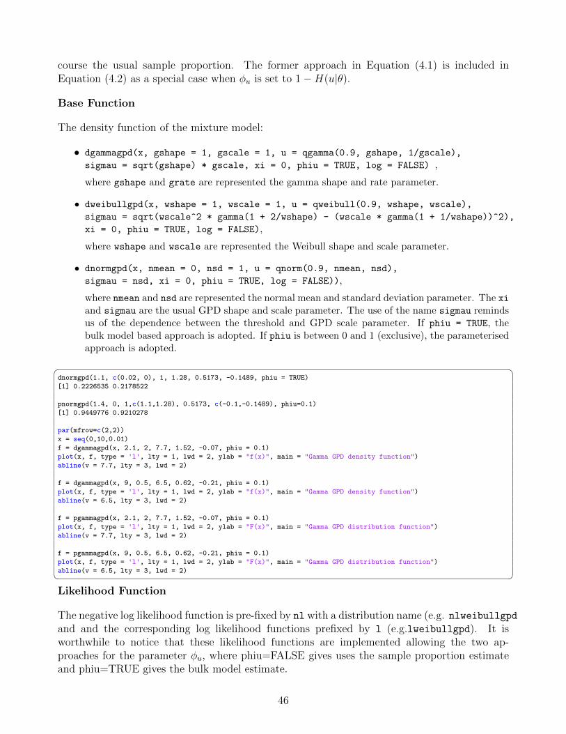
course the usual sample proportion. The former approach in Equation (4.1) is included inEquation (4.2) as a special case when φu is set to 1−H(u|θ).
Base Function
The density function of the mixture model:
• dgammagpd(x, gshape = 1, gscale = 1, u = qgamma(0.9, gshape, 1/gscale),
sigmau = sqrt(gshape) * gscale, xi = 0, phiu = TRUE, log = FALSE) ,
where gshape and grate are represented the gamma shape and rate parameter.
• dweibullgpd(x, wshape = 1, wscale = 1, u = qweibull(0.9, wshape, wscale),
sigmau = sqrt(wscale^2 * gamma(1 + 2/wshape) - (wscale * gamma(1 + 1/wshape))^2),
xi = 0, phiu = TRUE, log = FALSE),
where wshape and wscale are represented the Weibull shape and scale parameter.
• dnormgpd(x, nmean = 0, nsd = 1, u = qnorm(0.9, nmean, nsd),
sigmau = nsd, xi = 0, phiu = TRUE, log = FALSE)),
where nmean and nsd are represented the normal mean and standard deviation parameter. The xiand sigmau are the usual GPD shape and scale parameter. The use of the name sigmau remindsus of the dependence between the threshold and GPD scale parameter. If phiu = TRUE, thebulk model based approach is adopted. If phiu is between 0 and 1 (exclusive), the parameterisedapproach is adopted.
� �dnormgpd(1.1, c(0.02, 0), 1, 1.28, 0.5173, -0.1489, phiu = TRUE)
[1] 0.2226535 0.2178522
pnormgpd(1.4, 0, 1,c(1.1,1.28), 0.5173, c(-0.1,-0.1489), phiu=0.1)
[1] 0.9449776 0.9210278
par(mfrow=c(2,2))
x = seq(0,10,0.01)
f = dgammagpd(x, 2.1, 2, 7.7, 1.52, -0.07, phiu = 0.1)
plot(x, f, type = 'l', lty = 1, lwd = 2, ylab = "f(x)", main = "Gamma GPD density function")
abline(v = 7.7, lty = 3, lwd = 2)
f = dgammagpd(x, 9, 0.5, 6.5, 0.62, -0.21, phiu = 0.1)
plot(x, f, type = 'l', lty = 1, lwd = 2, ylab = "f(x)", main = "Gamma GPD density function")
abline(v = 6.5, lty = 3, lwd = 2)
f = pgammagpd(x, 2.1, 2, 7.7, 1.52, -0.07, phiu = 0.1)
plot(x, f, type = 'l', lty = 1, lwd = 2, ylab = "F(x)", main = "Gamma GPD distribution function")
abline(v = 7.7, lty = 3, lwd = 2)
f = pgammagpd(x, 9, 0.5, 6.5, 0.62, -0.21, phiu = 0.1)
plot(x, f, type = 'l', lty = 1, lwd = 2, ylab = "F(x)", main = "Gamma GPD distribution function")
abline(v = 6.5, lty = 3, lwd = 2)� �Likelihood Function
The negative log likelihood function is pre-fixed by nl with a distribution name (e.g. nlweibullgpdand and the corresponding log likelihood functions prefixed by l (e.g.lweibullgpd). It isworthwhile to notice that these likelihood functions are implemented allowing the two ap-proaches for the parameter φu, where phiu=FALSE gives uses the sample proportion estimateand phiu=TRUE gives the bulk model estimate.
46

Figure 4.1: The density function of the parametric form GPD mixture model showing that itmay have a discontinuity at the threshold. However, the corresponding distribution function (orCDF) is always continuous at the threshold. The vertical dashed line indicates the threshold.
An example of the syntax for the negative log likelihood function is explicitly designed for use inthe optimisation, so all the parameters are input as a vector (except φu) and is just a wrapperfor the likelihood function itself::
• nlgammagpd(pvector, x, phiu = TRUE, finitelik = FALSE), pvector has 5 arguments withgamma shape, gamma scale, threshold, GPD scale and GPD shape respectively.
The log likelihood function is pre-fixed by l with a distribution name (e.g. lweibullgpd andlnormgpd). The log likelihood function syntax is similar to that of the usual distribution func-tions::
• lgammagpd(x, gshape = 1, gscale = 1, u = qgamma(0.9, gshape, 1/gscale), sigmau =
sqrt(gshape) * gscale, xi = 0, phiu = TRUE, log = TRUE)
Now x is the data and phiu is the logical input indicating either parameterised approach orbulk model based approach. If let phiu = TRUE, the likelihood function will apply the bulkmodel based approach. If phiu = FALSE, the likelihood function will adopt the parameterisedapproach, and estimate phiu using the sample proportion above the threshold.
Fitting Function
The maximum likelihood based fitting function is pre-fixed by f with a distribution name (e.g.fweibullgpd). An example of the syntax for the MLE fitting function of the mixture model:
47

• fgammagpd(x, phiu = TRUE, pvector = NULL, std.err = TRUE, method = "BFGS",
control = list(maxit = 10000), finitelik = TRUE, ...),
The pvector is a vector of initial values of the mixture model and when pvector = NULL thenthe default initial values are used. x is a vector of sample data. The default value for phiu
= TRUE so that the tail fraction is specified by gamma distribution φu = 1 − H(.|θ), whereH(.|θ) could be parametric distribution function. When phiu = FALSE then the tail fraction istreated as an extra parameter estimated using the MLE which is the sample proportion abovethe threshold. std.err is a logical variable, if std.err = TRUE, then the standard errors of themodel parameters are calculated. finitelik is a logical variable, if finitelik = TRUE, thenlog-likelihood returns finite value for invalid parameters. The default optimisation algorithm is“BFGS”, which requires a finite negative log-likelihood function evaluation finitelik = TRUE.For invalid parameters, a zero likelihood is replaced with exp(-1e6). The “BFGS” optimisationalgorithms require finite values for likelihood, so any user input for finitelik will be overriddenand set to finitelik = TRUE if either of these optimisation methods is chosen. The method,control and ... are optional inputs passed to optim.
Examples
An example program for fitting a parametric bulk model is now given in Figures 4.2. The fitaround the threshold are rather different.� �x = rgamma(1000, shape = 2)
xx = seq(-1, 10, 0.01)
y = dgamma(xx, shape = 2)
par(xaxs="i", yaxs="i")
# Bulk model base tail fraction
fit = fgammagpd(x, phiu = TRUE, std.err = FALSE)
hist(x, breaks = 100, freq = FALSE, xlim = c(0, 10))
lines(xx, y)
lines(xx, dgammagpd(xx, gshape = fit$gshape, gscale = fit$gscale, u = fit$u,sigmau = fit$sigmau, xi = fit$xi, phiu = TRUE), col="red")
abline(v = fit$u)
# Parameterised tail fraction
fit2 = fgammagpd(x, phiu = FALSE, std.err = FALSE)
plot(xx, y, type = "l")
lines(xx, dgammagpd(xx, gshape = fit$gshape, gscale = fit$gscale, u = fit$u,sigmau = fit$sigmau, xi = fit$xi, phiu = TRUE), col="red")
lines(xx, dgammagpd(xx, gshape = fit2$gshape, gscale = fit2$gscale, u = fit2$u,sigmau = fit2$sigmau, xi = fit2$xi, phiu = fit2$phiu), col="blue")
abline(v = fit$u, col = "red")
abline(v = fit2$u, col = "blue")
legend("topright", c("True Density","Bulk T. F","Parameterised T. F"),
col=c("black", "red", "blue"), lty = 1, cex= 0.8)� �4.3.2 Gamma/Normal/Weibull/Log-Normal/Beta GPD with Single
Continuity Constraint Mixture Model
The continuity constraint is achieved by equating the bulk distribution and tail model at thethreshold and replacing the GPD scale parameter in terms of other parameters. For the mixtureextreme value models, the postfixes con means a continuity constraint at the threshold. For
48

Figure 4.2: Density function of the parametric extreme value mixture model with gamma forbulk with bulk and parameterised tail fraction approach, where the vertical line indicates thethreshold. A sample of size 1000 from a gamma distribution(2,1) is generated.
Figure 4.3: Example of density function and distribution function for continuous Weibull GPDdistribution, where the Weibull shape parameter is 2, the scale parameter is 0.5, the thresholdis fixed at 0.75 and GPD shape is -0.13. The blue line indicates the threshold.
example, the Weibull distribution is defined as weibull in R, so the quantile function for WeibullGPD model with continuity constraint is therefore abbreviated as qweibullgpdcon.
In the Figure 4.3, the Weibull shape parameter is 2, the scale parameter is 0.5, the thresholdis fixed at 0.75 and GPD shape is -0.13. It can be seen that not only the density function forthis mixture model is continuous at the threshold and distribution function will be continuousin first derivative.
49

Base Function
The base functions of the parametric form continuous mixture model have very similar set upwith the functions of parametric form mixture model, so will not be demonstrated again.
Examples of the syntax of the density function of parametric form continuous mixture model:
• dgammagpdcon(x, gshape = 1, gscale = 1, u = qgamma(0.9, gshape, 1/gscale), xi = 0,
phiu = TRUE, log = FALSE), As usual, phiu can represent either bulk model based approachor parameterised approach.
Fitting and Likelihood Function
The fitting and likelihood functions of the continuity constraint mixture model has very similarset up with the fitting function of parametric form mixture model. Hence, the basic use of thesefunctions will not be demonstrated again.
4.3.3 GPD-Normal-GPD (GNG) Model
Zhao et al. (2010) proposed a two tail mixture model, where the normal distribution describesthe bulk and the GPD has been fitted to both tails separately. The parameter vector is Θ =(µ, β, ul, σul , ξl, ur, σur , ξr).
Bulk Model Based Tail Fraction Approach
The distribution function is defined as:
F (x|Θ) =
φul {1−G(−x| − ul, σul , ξl)} x < ul,
H(x|µ, β) ul ≤ x ≤ ur,
(1− φur) + φurG(x|ur, σur , ξr) x > ur,
where φul = H(ul|µ, β) and φur = 1 − H(ur|µ, β) and H(.|µ, β) is the normal distributionfunction with mean µ and standard deviation β. G(.| − ul, σul , ξl) and G(.|ur, σur , ξr, ) are GPDdistribution functions for lower tail and upper tail.
Parameterised Tail Fraction Approach
It is possible to define φul = P (X < ul) and φur = P (X > ur). The corresponding distributionfunction is given by:
F (x|Θ) =
φul {1−G(−x| − ul, σul , ξl)} x < ul,
φul + (1− φul − φur)H(x|µ, β)−H(ul|µ, β)
H(ur|µ, β)−H(ul|µ, β)ul ≤ x ≤ ur,
(1− φur) + φurG(x|ur, σur , ξr) x > ur,
Base function
The example of the density function of GNG model.
50
• dgng(x, nmean = 0, nsd = 1,
ul = qnorm(0.1, nmean, nsd), sigmaul = nsd, xil = 0, phiul = TRUE,
ur = qnorm(0.9, nmean, nsd), sigmaur = nsd, xir = 0, phiur = TRUE, log = FALSE),
The xil and sigmaul are GPD shape and scale parameter for the lower tail and the correspond-ing value xir and sigmaur for the upper tail.� �f = dgng(x, 0, 1, -1.28, 0.42, 0.2, phiul = TRUE, 1.28, 0.42, 0.2, phiur = TRUE)
plot(x, f, ylim = c(0, 0.5), type = 'l', lty = 1, ylab = "Density", main = "GNG density function")
abline(v = -1.28, col = "blue")
abline(v =1.28, col = "blue")
f1 = dgng(x, 0, 1, -1.28, 0.6, -0.11, phiul = TRUE, 1.28, 0.6, -0.12, phiur = TRUE)
plot(x, f1, ylim = c(0, 0.5), type = 'l',lty = 1, ylab = "Density", main = "GNG density function")
abline(v = -1.28, col = "blue")
abline(v = 1.28, col = "blue")� �
Figure 4.4: Example of the density function of GNG model. The parameter vector is Θ =(µ = 0, β = 1, ul = −1.28, σul = 0.42, ξl = 0.2, ur = 1.28, σur = 0.42, ξr = 0.2) on left andΘ = (µ = 0, β = 1, ul = −1.28, σul = 0.6, ξl = −0.11, ur = 1.28, σur = 0.6, ξr = 0.12) onright. This example shows the density function of GNG could have continuity / discontinuityconstraints at either lower or upper threshold with different choices of parameter values.
An example of the density function of GNG model is given in Figure 4.4. The density functionmay have a discontinuity at either the lower threshold ul or the upper threshold ur.
Likelihood and Fitting Function
The fitting and likelihood functions are similar to those of the single tailed models, with theonly difference that they now take parameters for both tails and the tail fraction can take eitherparameterisation for both tails.
Examples
51

Figure 4.5 provides an example of simulated data with overlaid fitted gng and normgpd model.It shows that two tailed model provides more flexibility in fitting asymmetry data.� �x = rnorm(1000)
xx = seq(-5, 5, 0.01)
y = dnorm(xx)
# Bulk model base tail fraction
fit = fgng(x, phiul = TRUE, phiur = TRUE, std.err = FALSE)
hist(x, breaks = 100, freq = FALSE, xlim = c(-5, 5), main = "N(0, 1)")
lines(xx, dgng(xx, nmean = fit$nmean, nsd = fit$nsd,ul = fit$ul, sigmaul = fit$sigmaul, xil = fit$xil, phiul = TRUE,
ur = fit$ur, sigmaur = fit$sigmaur, xir = fit$xir, phiur = TRUE), col="blue", lwd = 2)
abline(v = c(fit$ul, fit$ur))legend('topright', 'gng',
col = "blue", lty =1, lwd = 2)
# Two tail model is safest if bulk has lower tail which is not normal tail
x = rt(3000, df = 3)
xx = seq(-10, 10, 0.01)
y = dt(xx, df = 3)
hist(x, breaks = 100, freq = FALSE, xlim = c(-10, 10), ylim= c(0, 0.5), main = "T (df=3)")
fit = fnormgpd(x, phiu = FALSE, std.err = FALSE)
fit2 = fgng(x, phiul = FALSE, phiur = FALSE, std.err = FALSE)
lines(xx, dnormgpd(xx, nmean = fit$nmean, nsd = fit$nsd,u = fit$u, sigmau = fit$sigmau, xi = fit$xi, phiu = fit$phiu), col="red", lwd = 2)
lines(xx, dgng(xx, nmean = fit2$nmean, nsd = fit2$nsd,ul = fit2$ul, sigmaul = fit2$sigmaul, xil = fit2$xil, phiul = fit2$phiul,ur = fit2$ur, sigmaur = fit2$sigmaur, xir = fit2$xir, phiur = fit2$phiur), col="blue", lwd = 2)
legend('topright', c("gng", "normgpd"), col = c("blue", "red"), lty =1, lwd = 2)� �4.3.4 GNG with Single Continuity Constraint Model
The continuity constraints are achieved by equating the normal distribution with the GPD atthe lower and upper threshold. The GPD scale parameters of the both tails are replaced by theother parameters. The function names are post-fixed by dgngcon, pgngcon, qgngcon, rgngcon torepresent corresponding density, distribution, quantile and random number generation functionrespectively.
Those functions from the GNG continuous mixture model have very similar set up with thefunctions of GNG model. Hence, the details of these functions will not repeat again.
4.3.5 Dynamically Weighted Mixture Model
Frigessi et al. (2002) suggested a dynamically weighted mixture model by combining the Weibullfor the bulk model with GPD for the tail model. Instead of explicitly defining the threshold, theyuse a Cauchy cumulative distribution function for the mixing function to make the transitionbetween the bulk distribution and tail distribution.The density function of the dynamic mixture model is given by:
l(x) =[1− p(x|θ)] f(x|β) + p(x|θ)g(x|0, σu, ξ)
Z(θ, β, σu, ξ),
where f(x|β) denotes the Weibull density and Z(θ, β, σu, ξ) denotes the normalizing constant tomake the density integrate to one. The mixing function p(.|θ) is a Cauchy distribution functionwith location parameter µ and scale parameter τ .
52

Figure 4.5: Left: The example of 1000 simulated data from a standard normal distribution withoverlaid fitted GNG model with parameter vector (µ = −0.049, β = 0.971, ul = −1.347, σul =0.519, ξl = −0.170, ur = 1.191, σur = 0.637, ξr = −0.223). Right: The example of 3000 simu-lated data from Student-t(3) distribution with overlaid fitted normgpd and GNG model withparameter vector (µ = 0.455, β = 1.792, u = 1.729, σu = 0.940, ξ = 0.394) and (µ = −0.005, β =0.994, ul = −1.778, σul = 0.888, ξl = 0.318, ur = 1.687, σur = 0.913, ξr = 0.396), respectively.
Base Function
This dynamic weighted mixture distribution is abbreviated as dwm and an example of the syntaxis given by:
• ddwm(x, wshape = 1, wscale = 1, cmu = 1, ctau = 1,
sigmau = sqrt(wscale^2 * gamma(1 + 2/wshape) - (wscale * gamma(1 + 1/wshape))^2),
xi = 0, log = FALSE),
As before, the wshape and wscale are the Weibull shape and scale parameters. cmu and ctau
are Cauchy distribution location and scale parameter. The quantile function qdwm requires thenumerical integration of the distribution function pdwm, which very rarely fails due to integrationdifficulties. Further, the quantile function is not available in close form so require numericalinversion, which can also fail. The argument qinit is the initial quantile estimate, which can beused in case of failure. Hence, the parameter qinit is set up for user to choose some reasonableinitial values for the quantile function.
An example of the three components and the resultant density estimate are given in Figure 4.6,which reproduces the example given in Frigessi et al. (2002).� �xx = seq(0.001, 5, 0.01)
f = ddwm(xx, wshape = 2, wscale = 1/gamma(1.5), cmu = 1, ctau = 1, sigmau = 1, xi = 0.5)
plot(xx, f, ylim = c(0, 1), xlim = c(0, 5), type = 'l', lwd = 2,
53

Figure 4.6: Reproduce the plot examples of the dynamically weighted mixture model fromFrigessi et al. (2002) in page 226, where the parameter vector Θ = (wshape = 2, wscale =1.128, cmu = 1, ctau = 1, sigmau = 1, xi = 0.5).
ylab = "density", main = "Plot example in Frigessi et al. (2002)")
lines(xx, dgpd(xx, xi = 1, sigmau = 0.5), col = "red", lty = 2, lwd = 2)
lines(xx, dweibull(xx, shape = 2, scale = 1/gamma(1.5)), col = "blue", lty = 2, lwd = 2)
legend('topright', c('DWM', 'Weibull', 'GPD'),col = c("black", "blue", "red"), lty = c(1, 2, 2), lwd = 2)� �
Fitting and Likelihood Function
The fitting and likelihood functions are similar with other models so is not discussed here.
Examples
Figure 4.7 provides an example of simulated Weibull data with overlaid fitted dynamic weightedmixture model.� �x = rweibull(1000, shape = 2, scale = 1.5)
xx = seq(0.1, 5, 0.01)
fit = fdwm(x, std.err = FALSE)
hist(x, 100, freq = FALSE, ylim = c(0, 1.3), main =" dwm example")
lines(xx, ddwm(xx, wshape = fit$wshape, wscale = fit$wscale, cmu = fit$cmu, ctau = fit$ctau,sigmau = fit$sigmau, xi = fit$xi),lwd=2)
lines(xx, dgpd(xx, sigmau = fit$sigmau, xi = fit$xi), col = "red", type = 'l', lwd = 2)
lines(xx, dweibull(xx, shape = fit$wshape, scale = fit$wscale), col = "blue", lwd = 2)
lines(xx, pcauchy(xx, location = fit$cmu, scale = fit$ctau), col = "green", lty = 2, lwd = 2)
legend("topleft", c("dwm", "GPD", "Weibull", "Cauchy"), col = c("black", "red", "blue", "green")� �54

Figure 4.7: Example of 1000 simulated data from a Weibull(2,1.5) distribution with overlaidfitted dynamic weighted mixture model with parameter vector Θ = (wshape = 1.993, wscale =1.530, cmu = 2.901, ctau = 0.001, sigmau = 1.027, xi = −0.145).
4.3.6 Hybrid Pareto Model
Carreau and Bengio (2008) proposed a hybrid Pareto model by splicing a normal distributionwith GPD and set continuity constraint on the density and on its first derivative at the threshold.However, with a key difference to the usual mixture from Section 4.3.1 to Section 4.3.5 that it doesnot treat the GPD a conditional model, so the tail fraction scaling of the GPD φu = P (x > u) isnot included. The unscaled GPD is simply spliced with the normal truncated at the threshold, sothe density needs to be renormalized as it gets the contribution from the truncated normal uptothe threshold and the entire unit integration of the GPD above the threshold.. The parametershave to adjust for the lack of tail fraction scaling. The GPD scale σu and threshold u areparameterised the other parameters to achieve two continuous constraints. Hence, they havereduced the initial 5 parameters to the normal mean µ and standard deviation β with the GPDshape ξ. The parameter vector is θ = (µ, β, ξ). The hybrid Pareto mixture density is defined as:
f(x|θ) =
1
τh(x|µ, β) x ≤ u,
1
τg(x|u, σu, ξ) x > u.
µ is the normal mean and β is the standard deviation parameter. h(.|µ, β) is the normal densityfunction and g(.|u, σu, ξ) is the GPD density function. The τ is the usual normalising constantand τ = 1 +H(u|µ, β), where the 1 comes from the integration of the unscaled GPD and secondterm is from the usual normal component.
The condmixt package written by one of the original authors of the hybrid Pareto model (Carreau
55

and Bengio (2008)) also has similar functions for the hybrid Pareto hpareto and mixture ofhybrid Paretos hparetomixt, which are more flexible as they also permit the model to betruncated at zero.
Base Function
The hybrid Pareto distribution is abbreviated as hpd. Hence, the corresponding functions aredefined as:
• dhpd(x, nmean = 0, nsd = 1, xi = 0, log = FALSE),
Likelihood and Fitting Function
Examples
Figure 4.8 demonstrates that the hybrid Pareto cannot provide a reasonable fit for the normaldistribution but normgpdcon model could give a better fit.
Figure 4.8: Example of 1000 simulated data from a standard normal distribution with overlaidfitted hpd model with parameter vector of (µ = −0.606, β = 0.614, ξ = −0.372) and normgpdcon
model with parameter vector of (µ = −0.015, β = 1.001, u = 1.987, ξ = −0.089).
The negative log likelihood function of hpd is named as nlhpd and log likelihood function isnamed as lhpd. Similarly, the fitting function of hpd is named as fhpd. These functions havesimilar set up with other mixture models, so they are not detailed again.� �x = rnorm(1000)
xx = seq(-4, 4, 0.01)
y = dnorm(xx)
# Hybrid Pareto provides reasonable fit for asymmetric heavy tailed distribution
# but not for cases such as the normal distribution
fit = fhpd(x, std.err = FALSE)
hist(x, breaks = 100, freq = FALSE, xlim = c(-4, 4))
lines(xx, dhpd(xx, nmean = fit$nmean, nsd = fit$nsd,
56

xi = fit$xi), col="red", lwd = 2)
abline(v = fit$u, col="red", lwd = 2)
# Notice that if tail fraction is included a better fit is obtained
fit2 = fnormgpdcon(x, std.err = FALSE)
lines(xx, dnormgpdcon(xx, nmean = fit2$nmean, nsd = fit2$nsd, u = fit2$u,xi = fit2$xi), col="blue", lwd = 2)
abline(v = fit2$u, col="blue", lwd = 2)
legend("topright", c("hpd", "normgpdcon" ), col = c("red", "blue")� �4.3.7 Hybrid Pareto with Single Continuous Constraint Model
A similar model can be suggested by splicing a normal distribution with GPD and set a continuityconstraint on the density only not constraining it to also be continuous in first derivative at thethreshold. The initial 5 parameters haven been reduced to threshold u, normal mean µ, standarddeviation β and GPD shape ξ, which is consistent with previous continuity model. Again, notethat the a key difference that φu is not included in this model, so there is no scaling of uppertail and bulk model. The parameter vector is θ = (u, µ, β, ξ). The single continuous constrainthybrid Pareto mixture density is defined as:
f(x|θ) =
1
τh(x|µ, β) x ≤ u,
1
τg(x|u, σu, ξ) x > u,
where h(.|µ, β) is the normal density function and GPD density function is defined as g(.|u, σu, ξ).The τ is the usual normalising constant and τ = 1 + H(u|µ, β), where the 1 comes from theintegration of the unscaled GPD and second term is from the usual normal component.
Base Function
The standard density, distribution , quantile, random number generation functions of the singlecontinuous constraint hybrid Pareto model are similar with the original hybrid Pareto. Theexample of density function of single continuous constraint hybrid Pareto model:
• dhpdcon(x, nmean = 0, nsd = 1, u = qnorm(0.9, nmean, nsd), xi = 0, log = FALSE)
Likelihood and Fitting Function
An example of fitting the hybrid Pareto (with and without the constraint of continuous firstderivative) and the normal with GPD tail with single continuity constraint is given below.
Examples
Figure 4.9 demonstrates that two hybrid Pareto models cannot provide a reasonable fit for thenormal distribution but normgpdcon model could give a better fit.� �x = rnorm(1000)
xx = seq(-4, 4, 0.01)
y = dnorm(xx)
# Two Hybrid Pareto models provide reasonable fit for asymmetric heavy tailed distribution
57

Figure 4.9: Left: Example of 1000 simulated data from a normal distribution with overlaidfitted hpd model with parameter vector of (µ = −0.606, β = 0.614, ξ = −0.372), and hpdcon
model with parameter vector of (µ = −0.547, β = 0.651, u = −0.558, ξ = −0.472). Right:Example of 1000 simulated data from a normal distribution with overlaid fitted hpdcon modelwith parameter vector of (µ = −0.547, β = 0.651, u = −0.558, ξ = −0.472) and normgpdcon
model with parameter vector of (µ = 0.007, β = 0.970, u = 1.315, ξ = −0.255).
# but not for cases such as the normal distribution
fitcon = fhpdcon(x, std.err = FALSE)
fit = fhpd(x, std.err = FALSE)
hist(x, breaks = 100, freq = FALSE, xlim = c(-4, 4))
lines(xx, dhpdcon(xx, nmean = fitcon$nmean, nsd = fitcon$nsd, u = fitcon$u,xi = fitcon$xi), col="darkgreen", lwd = 2)
abline(v = fitcon$u, col="darkgreen", lwd = 2)
lines(xx, dhpd(xx, nmean = fit$nmean, nsd = fit$nsd, xi = fit$xi), col="red", lwd = 2)
abline(v = fit$u, col="red", lwd = 2)
legend("topleft", c("hpdcon", "hpd" ), col = c("darkgreen", "red")
,lty = c(1, 1), lwd = c(2, 2))
# Notice that if tail fraction is included a better fit is obtained
fit2 = fnormgpdcon(x, std.err = FALSE)
hist(x, breaks = 100, freq = FALSE, xlim = c(-4, 4))
lines(xx, dnormgpdcon(xx, nmean = fit2$nmean, nsd = fit2$nsd, u = fit2$u,xi = fit2$xi), col="blue", lwd = 2)
lines(xx, dhpdcon(xx, nmean = fitcon$nmean, nsd = fitcon$nsd, u = fitcon$u,xi = fitcon$xi), col="darkgreen", lwd = 2)
abline(v = fit2$u, col="blue", lwd = 2)
abline(v = fitcon$u, col="darkgreen", lwd = 2)
legend("topleft", c("hpdcon", "normgpdcon" ), col = c("darkgreen", "blue")� �4.4 Non-Parametric Mixture Models
MacDonald et al. (2011) and MacDonald et al. (2013) developed a non-parametric kernel densityestimator based extreme value mixture models extending on that developed by Tancredi et al.
58

(2006). The former has been implemented in the first version of this package.
4.4.1 Kernel GPD Model
MacDonald et al. (2011) constructed a standard kernel density estimator as the bulk modelbelow the threshold with GPD for the tail model. The distribution function of standard kernelGPD mixture model is given by:
Bulk Model Based Tail Fraction Approach
F (x|X,λ, u, σu, ξ, φu) =
{H(x|X,λ) x ≤ u,(1− φu) + φu ×G(x|u, σu, ξ) x > u,
where φu = 1−H(u|X,λ).
Parameterised Tail Fraction Approach
F (x|X,λ, u, σu, ξ, φu) =
{(1− φu)H(x|X,λ)
H(u|X,λ)x ≤ u,
(1− φu) + φu ×G(x|u, σu, ξ) x > u,
where H(.|X,λ) is the distribution function of the kernel density estimator and G(.|u, σu, ξ) isthe distribution function of GPD. The traditional kernel density estimator is defined as:
h(x; X, λ) =1
nλ
n∑i=1
K
(x− xiλ
),
where K(.) is the kernel function and usually to be a symmetric and unimodal probabilitydensity function and lambda is the bandwidth parameter. The kernel function usually meetsthe following conditions: K(x) ≥ 0 and
∫K(x) dx = 1.
Base Function
The density function of kernel GPD model is given by:
• dkdengpd(x, kerncentres, lambda = NULL, u = as.vector(quantile(kerncentres, 0.9)),
sigmau = sqrt(6*var(kerncentres))/pi, xi = 0, phiu = TRUE, log = FALSE)
where lambda is the bandwidth parameter of the kernel density estimator and kerncentres is thesample of data. The phiu can be used for determining either bulk model based or parameterisedapproach.
Likelihood Function
The negative log likelihood and log likelihood functions are pre-fixed as usual:
• nlkdengpd(pvector, x, phiu = TRUE, finitelik = FALSE)
• lkdengpd(x, lambda = NULL, u = 0, sigmau = 1, xi = 0, phiu = TRUE, log = TRUE)
59

Fitting Function
Notice that the kernel centres are not needed in the likelihood functions as these are the data.
Two important practical issues arise with MLE for the kernel bandwidth:
• Cross-validation likelihood is needed for the kernel density estimator bandwidth parameteras the usual likelihood degenerates by Habbema et al. (1974) and Duin (1976). If the datahas been heavily rounded, the bandwidth can be zero even if the using cross-validationlikelihood. To overcome this issue an option to add a small jitter to the data has beenincluded in the fitting inputs, using the jitter function, to remove the ties.
• For heavy tailed populations, the bandwidth is positively biased, giving a larger bandwidth.One solution to this problem is to splice the GPD to both the upper and lower tails (usingthe gkg function discussed below), as the bias comes from the lack of separation of theupper and lower order statistics in the two tails
The fitting function is given by:
• fkdengpd(x, phiu = TRUE, pvector = NULL, add.jitter = FALSE, factor = 0.1,
amount = NULL, std.err = TRUE, method = "BFGS",
control = list(maxit = 10000), finitelik = TRUE, ...)
x is a vector of sample data. add.jitter is a logical variable, if add.jitter = TRUE, thenthe jitter is needed for rounded data. factor and amount are the arguments passed to theadd.jitter.
ExamplesAn example program for fitting the kernel GPD model is now given in Figures 4.10, whichhighlights the usefulness of this model.� �x = rnorm(1000, 0, 1)
fit = fkdengpd(x, phiu = FALSE, std.err = FALSE)
hist(x, 100, freq = FALSE, xlim = c(-4, 4))
xx = seq(-4, 4, 0.01)
lines(xx, dkdengpd(xx, x, fit$lambda, fit$u, fit$sigmau, fit$xi, fit$phiu), col="blue", lwd = 2)
abline(v = fit$u, col="blue", lwd = 2)
legend("topright", "kdengpd", col = "blue",
,lty = 1, lwd = 2)
# Try a bimodal data
x <- c(rnorm(1000,-1,0.7),rnorm(1000,3,1))
fit = fkdengpd(x, phiu = FALSE, std.err = FALSE)
hist(x, 100, freq = FALSE, xlim = c(-4, 6.5), main="Bimodal data example")
xx = seq(-5, 6, 0.001)
lines(xx, dkdengpd(xx, x, fit$lambda, fit$u, fit$sigmau, fit$xi, fit$phiu), col="blue", lwd = 2)
abline(v = fit$u, col="blue", lwd = 2)
legend("topright", "kdengpd", col = "blue",
,lty = 1, lwd = 2)� �4.4.2 Two Tailed Kernel GPD Model
MacDonald et al. (2011) introduced a two tailed mixture model by splicing the standard kerneldensity estimator with two extreme value tail models. This two-tailed extreme value mixture
60

Figure 4.10: Left: Example of 1000 simulated data from a standard normal distribution withoverlaid fitted kdengpd model with parameter vector of (λ = 0.305, u = 1.048, σu = 0.522, ξ =−0.117). Right: Example of 2000 simulated data from a mixture of standard normals withoverlaid fitted kdengpd model with parameter vector of (λ = 0.201, u = 3.536, σu = 0.759, ξ =−0.260).
model also overcomes the inconsistency in the cross-validation likelihood estimation of the band-width for heavy tailed distributions, see MacDonald et al. (2011) for details.
The parameter vector is Θ = (X,λ, u1, σul , ξl, φul , u2, σur , ξr, φur). The distribution function oftwo tailed mixture model is given by:Parameterised Tail Fraction Approach
F (x|Θ) =
φul {1−G(−x| − ul, σul , ξl)} x < ul,
φul + (1− φul − φur)H(x|X,λ)−H(ul|X,λ)
H(ur|X,λ)−H(ul|X,λ)ul ≤ x ≤ ur,
(1− φur) + φurG(x|ur, σur , ξr) x > ur,
where φul and φur are estimated as the sample proportions less than threshold ul and above thethreshold ur respectively. G(−x| − ul, σul , ξl) is the unconditional GPD function for x < ul andG(x|ur, σur , ξr) is the unconditional GPD function for x > ur.
Bulk Model Based Tail Fraction Approach
F (x|Θ) =
φul {1−G(−x| − ul, σul , ξl)} x < ul,
H(x|X,λ) ul ≤ x ≤ ur,
(1− φur) + φurG(x|ur, σur , ξr) x > ur,
61

where φul=H(ul, X, λ) and φur = 1−H(ur, X, λ).
Base FunctionThe density function of two tailed kernel GPD model is defined as:
• dgkg(x, kerncentres, lambda = NULL,
ul = as.vector(quantile(kerncentres, 0.1)), sigmaul = sqrt(6*var(kerncentres))/pi,
xil = 0, phiul = TRUE,
ur = as.vector(quantile(kerncentres, 0.9)), sigmaur = sqrt(6*var(kerncentres))/pi,
xir = 0, phiur = TRUE, log = FALSE),
The basic use of the standard function will not repeated again.
Likelihood and Fitting Function
The likelihood and fitting functions are defined as usual:
• nlgkg(pvector, x, phiul = TRUE, phiur = TRUE, finitelik = FALSE)
• lgkg(x, lambda = NULL,
ul = as.vector(quantile(x, 0.1)), sigmaul = 1, xil = 0, phiul = TRUE,
ur = as.vector(quantile(x, 0.9)), sigmaur = 1, xir = 0, phiur = TRUE, log = TRUE)
• fgkg(x, phiul = TRUE, phiur = TRUE, pvector = NULL, add.jitter = FALSE,
factor = 0.1, amount = NULL, std.err = TRUE, method = "BFGS",
control = list(maxit = 10000), finitelik = TRUE, ...)
ExamplesAn example program for fitting the two tailed kernel GPD model is now given in Figures 4.11,which highlights the flexibility of this model.� �x = rt(1000, 3, 1)
fit = fgkg(x, phiul = FALSE, phiur = FALSE, std.err = FALSE)
hist(x, 100, freq = FALSE, xlim = c(-8, 10))
xx = seq(-8, 10, 0.01)
lines(xx, dgkg(xx, x, fit$lambda, fit$ul, fit$sigmaul, fit$xil, fit$phiul, fit$ur, fit$sigmaur, fit$xir, fit$phiur), col="blue", lwd = 2)
abline(v = fit$ul, col="blue", lwd = 2)
abline(v = fit$ur, col="blue", lwd = 2)
legend("topright", "gkdeng", col = "blue",
,lty = 1, lwd = 2)
# Try a bimodal data
x <- c(rnorm(1000,-1,0.7),rnorm(1000,3,1))
fit = fgkg(x, phiul = FALSE, phiur = FALSE, std.err = FALSE)
hist(x, 100, freq = FALSE, xlim = c(-4, 6.5), main="Bimodal data example")
xx = seq(-4, 6.5, 0.01)
lines(xx, dgkg(xx, x, fit$lambda, fit$ul, fit$sigmaul, fit$xil, fit$phiul, fit$ur, fit$sigmaur, fit$xir, fit$phiur), col="blue", lwd = 2)
abline(v = fit$ul, col="blue", lwd = 2)
abline(v = fit$ur, col="blue", lwd = 2)
legend("topright", "gkdeng", col = "blue",
,lty = 1, lwd = 2)� �
62

Figure 4.11: Left: Example of 1000 simulated data from Student-t(3,1) distribution with withoverlaid fitted gkg model with parameter vector of (λ = 0.347, ul = −0.230, σul = 0.494, ξl =0.334, ur = 3.617, σur = 1.727, ξr = 0.171). Right: Example of 2000 simulated data from amixture of standard normal distributions with with overlaid fitted gkg model with parametervector of (λ = 0.233, ul = −1.565, σul = 0.472, ξl = −0.218, ur = 3.686, σur = 0.669, ξr =−0.225).
4.4.3 Boundary Corrected Kernel GPD Model
MacDonald et al. (2013) combine a boundary corrected kernel density estimator for bulk modelsliced at the threshold with a point process representation of GPD tail model. The bound-ary correction kernel density estimator tries to reduce the inherent bias of the kernel densityestimator. The distribution function of boundary corrected mixture model is given by:
Bulk Model Based Tail Fraction Approach
F (x|X, hBC , u, σu, ξ, φu) =
{HBC(x|X,λBC) x ≤ u,(1− φu) + φu ×G(x|u, σu, ξ) x > u,
where φu = 1−HBC(u|X, h).
Parameterised Tail Fraction Approach
F (x|X, hBC , u, σu, ξ, φu) =
{(1− φu)HBC(x|X,λBC)
HBC(u|X,λBC)x ≤ u,
(1− φu) + φu ×G(x|u, σu, ξ) x > u,
where HBC(x|X,λBC) is the distribution function of the boundary correction kernel densityestimator.
Base Function
The density functionis given by:
63
• dbckdengpd(x, kerncentres, lambda = NULL,
u = as.vector(quantile(kerncentres, 0.9)), sigmau = sqrt(6*var(kerncentres))/pi,
xi = 0, phiu = TRUE, bcmethod = "simple", proper = TRUE, nn = "jf96",
offset = 0, xmax = Inf, log = FALSE)
The density, distribution, quantile function of boundary corrected kernel GPD model have verysimilar set up with the standard kernel GPD model. Hence, the basic use of these functions willnot repeat here. See help(dbckdengpd) for details of boundary correction methods that havebeen implemented.
Likelihood and Fitting Function
The likelihood functions and fitting function are very similar with other mixture models.
• nlbckdengpd(pvector, x, phiu = TRUE, finitelik = FALSE)
• lbckdengpd(x, lambda = NULL, u = 0, sigmau = 1, xi = 0, phiu = TRUE, log = TRUE)
• fbckdengpd(x, phiu = TRUE, pvector = NULL, add.jitter = FALSE,
factor = 0.1, amount = NULL, bcmethod = "simple", proper = TRUE, nn = "jf96",
offset = 0, xmax = Inf, std.err = TRUE, method = "BFGS", control = list(maxit = 10000),
finitelik = TRUE, ...)
The basic use of these functions will not be detailed again.
64

Chapter 5
Simulation Study
5.1 Introduction
The simulation study is to assess the performance of the different extreme value mixture modelby approximating some standard parametric distributions. In particular, to focus on their per-formance for estimating tail quantiles. These population distributions are chosen to representexamples of symmetric and asymmetric behaviors with 3 types of lower and upper tail behaviors.Various mixture models can be classified as a single tail model with the full support, a singletail model with bounded positive support or two tail model with the full support. This studywill examine only the relevant population distributions for the suitable mixture model.
It is common practice that the population distribution can be referred to one of the three typesof distribution due to the limiting tail behaviors defined by the shape parameter ξ as type I(ξ = 0), type II (ξ > 0) and type III (ξ < 0). These three types of distribution have beenmentioned in chapter 2.
In the simulation study, 100 replicates with sample size 1000 or 5000 are simulated for eachdistribution. The estimated 90%, 95%, 99%, 99.9% quantiles of the single tailed extremalmixture models will be calculated to compare with true quantiles under different populationdistributions while the estimated 0.1%, 1%, 5%, 10%, 90%, 95%, 99% and 99.9% quantiles willbe calculated for the two tailed extremal mixture models. The RMSE (the root of mean squarederror) is then used for measuring the performance of the estimated quantile with true quantileat each population distribution. A 95% bootstrap percentile interval using 100,000 bootstrapsamples of the RMSE is obtained to explore evidence for the difference in performance.
It is expected that the estimated quantile tends to have higher uncertainty (higher RMSE) asthe quantile gets close to the tail of the distribution. The estimated quantile also tends to havelarger RMSE if the population distribution is heavy tailed. All population distributions in thissensitive analysis have a single mode and it is worth mentioning that non-parametric kerneldensity estimator based models and the mixture of gamma GPD model can cope with morecomplex data structure (e.g. bimodal or multimodal).
65

5.2 Simulation Parameters for Inference
The section will explain how the initial value of the parameters for likelihood optimisation orBayesian Inference MCMC were chosen.
5.2.1 Initial Value For The Likelihood Inference Based Model
The initial value of the parameter sometimes has a great impact on the likelihood inference asthe mixture models often have multiple local modes. In order to compare the model performancedifferences which are not caused by the sensitive initial values, it is reasonable to make a fewassumptions about the initial value of parameters. The initial threshold u is assumed as the 90%quantile of the data. According to the gpd.fit function from ismev package in R, the initial valuesfor the GPD shape ξ and scale σu parameter have been chosen as 0.1 and
√(6× var(data))/π
which is the standard deviation for the Gumbel case of the GEV distribution. Thus, thissimulation study follows this rule. The initial values for the bulk model are essentially selectedas the true value, assuming the bulk model extends over the entire range of support.
5.2.1.1 Optimization Method And Quantile Estimation
There are several different numerical methods to search for the MLE in R. The optim func-tion which includes various optimization routines has been adopted. The quasi-Newton based“BFGS” method is used in the simulation study.
The estimated parameters are plugged into the relevant quantile function for quantile inference.In order to make sure the likelihood function converges, the maximum number of iterations hasbeen changed to 20000. It is important to note that the parameters are only be used for quantileestimation when the likelihood function converges.
5.2.2 Initial Value for the Bayesian Inference Based Model
For the Bayesian inference is also evaluated for the kernel GPD and boundary corrected kernelGPD based extreme value mixture models, there are 5 parameters in the model including kernelbandwidth h, threshold u, point process shape ξpp, scale σ and location parameter µ. The pointprocess shape ξpp and GPD shape ξ are the same. The point process scale σ and GPD scaleparameters are related by σ = σu − ξ(u− µ).
The initial value of the threshold u is the 90% quantile for MCMC. The shape, scale and locationfor point process model are found by maximizing the point process log-likelihood function. Theinitial value for point process location parameter µ is set to equal 0.9*u. Moreover, the scalingvariable nb from the point process likelihood function is equal to number of data greater thanthe threshold, following the advice given by Wadsworth and Tawn (2012).
The initial value of the bandwidth is found by minimizing the asymptotic mean integratedsquared error (AMISE). When the normal distribution has been used as the kernel function, theoptimal choice of bandwidth for a normal population is given by:
h =
(4σ5
3n
)1/5
,
66

where n is refer to the number of data below the threshold u and σ is refer to the standarddeviation of the data below the threshold u. This rule refers as the Silverman’s Rule of Thumbor normal reference rule. Consequently, this formula gives the initial value of h for the MCMC.
5.2.2.1 Prior Information in Bayesian Inference
For Bayesian inference, we also need to provide the prior information about each parameter. Inorder to let the data speak for themselves, very diffuse priors have been used in the simulationstudy. The details of the prior structure of the kernel GPD model and boundary correctedkernel GPD model can be found in MacDonald et al. (2011) and MacDonald et al. (2013). Itis reasonable to assume that the prior for PP parameters (µ, σ, ξ) are independent with thethreshold u and the bandwidth parameter h:
π(h, u, µ, σ, ξ) = π(h)π(u)π(µ, σ, ξ).
The prior for the point process parameter, π(µ, σ, ξ), is a trivariate normal distribution witha large variances to indicate little prior information. Each point process parameter has beensuggested a mean of zero and a standard deviation of 100 except the PP scale parameter is ona log scale.
The prior for the bandwidth is based on an inverse gamma distribution (d1, d2) to specify theprecision parameter 1/h2, where d1 and d2 are the hyperparameters. Brewer (2000) suggests to
specify d1 > 0.5 and d2 =
[Γ(d1)
Γ(d1 − 0.5)
]2
.
The prior for the threshold is suggested by Behrens et al. (2004), which is a truncated normaldistribution truncate at the minimum of the data. The mean of the truncated normal distributionis the 90th quantile with standard deviation of
√12.
5.2.2.2 Quantile Calculation
The MCMC algorithm runs for 10000 iterations with a burn-in period of 1000, which resultinga 9000 posterior draws for each simulation. The posterior mean of the each parameter fromthe 9000 posterior draws is used to estimate the corresponding quantile. The quantile functionsfor the kernel GPD and boundary corrected GPD model require integrating the distributionfunction of kernel GPD or boundary corrected GPD, respectively. It is possible that for someposterior mean values, the integration could fail. In this case, another simulation will be carriedout.
5.3 A Single Tail Model With Full Support
This section will investigate different extremal mixture models including normal GPD mixture,continuous normal GPD mixture, standard kernel GPD, hybrid Pareto and single continuousconstraint hybrid Pareto model. The first three models can be implemented by either bulk modelbased tail fraction approach or parameterized tail fraction approach. Hence, these extremalmixture models can be classified into two groups:
67

• bulk model based tail fraction approach,
• parameterized tail fraction approach.
Five different populations will be considered in this case including normal(µ = 0, σ = 3), Student-t(v = 3, µ = 0), Gumbel(σ = 1), negative Weibull(l = 10, k = 5) and Student-t(v = 4, µ = 1)shown in Figure 5.1. These provide a wide range of upper tail and bulk features. Both normal(type I) and Student-t(v = 3, µ = 0) (type II) are symmetric distributions while Gumbel(σ = 1)is an asymmetric distribution with a type III lower tail and a type I upper tail and negativeWeibull(l = 10, k = 5) is an asymmetric distribution with a short lower and upper tail (typeIII). Student-t(v = 4, µ = 1) is an asymmetric distribution with a heavy lower and upper tail(type II) and the lower tail is not as heavy as the upper tail.
Figure 5.1: Population distributions used for the single tail full support model in the simulationstudy.
The 5 mixture models will be abbreviated as:
• CONnormGPD ⇒ the continuous constraint normal GPD mixture model;
• normGPD ⇒ the normal GPD mixture model;
• hPD ⇒ hybrid Pareto model;
68

• shPD ⇒ the single continuous constraint hybrid Pareto model;
• kernelGPD ⇒ the kernel density estimator GPD model.
5.3.1 Parameterised Tail Fraction Approach
The overall results show that the RMSE tends to get larger when the tail probability decreasesand the RMSE also become larger if the population distribution is heavy tail. It should benoticed that the model performance is only comparable under the same population distribution,as the RMSE generally increases with quantile level. High quantile estimates (99.9%) are fairlyrobust to the bulk model while the lower quantile estimates (90%, 95%, 99%) are more sensitiveto the choice of the bulk model. In fact, all 5 models have a similar bootstrap percentile intervalsand the associated intervals overlap with each other, which suggests that there are no significantmodel performance differences. This seems to suggest that for a sufficiently high quantile, theGPD will asymptotically dominate the upper tail while the distribution below the threshold nolonger contributes much at the level of extremity.
From Table 5.1, both hPD and shPD perform poorly in most population distributions at lowerquantile (90%, 95%, 99%), except the hPD works reasonably well for a Gumbel distribution at99% quantile. In particular hPD and shPD have very poor fit for symmetrical distributions.There is no overlap between the 95% bootstrap percentile confidence interval of the best fitmodel and the associated interval of the hPD or shPD, which confirms they are significant worsein terms of RMSE compared to the best mixture model for a given quantile (90%, 95%, 99%).When the sample size increase to 5000, from Table 5.2, the performance of the two hybrid Paretomodels (hPD and shPD) doesn’t improve. There is no significant improvement for two hybridPareto models when the population distribution sample size is 5000 as the RMSE gets largerin most cases of the lower quantile. Initially, it is surprising that the performance is so poorfor a normal distribution. Even though Carreau and Bengio (2008) propose the hPD modelby combing a normal and GPD and set two continuous constraints to make the the densityand first derivative continuous at the threshold, this model is different from the continuousconstraint normal GPD model (CONnormGPD). In particular with the key difference is thatthey ignore the usual tail fraction φu scaling of the conditional GPD, which means that theydon’t treat the GPD as a conditional model. Essentially the hPD seems to only perform well forcertain asymmetric distributions, but even this it does not work for the asymmetric non-centralt distribution considered here.
There are some interesting results from normal GPD model (normGPD) and continuous normalGPD model (CONnormGPD). For the Student-t(v = 3, µ = 0) and Student-t(v = 4, µ = 1)distribution, it seems that CONnormGPD performs better than normGPD as the RMSE ofthe CONnormGPD is smaller in general. No such conclusions can be drawn for the normaldistribution. It should be noted that the differences of the RMSE at different quantiles from twomodels are not likely to reach the level of a statistical significance. However, if the underlyingdistribution is Gumbel, it appears that normGPD outperforms CONnormGPD. There are nosignificant performance differences of these two models for a negative Weibull distribution (l =10, k = 5). When the sample size increases to 5000, the normGPD has achieved a significantreduction of RMSE in the 90%, 95%, 99% quantile of Gumbel distribution and 95%, 99%quantile at the negative Weibull compared with corresponding RMSE of CONnormGPD. These
69

suggest that the normGPD is more flexible than the CONnormGPD, which is obvious as theCONnormGPD restricts GPD scale parameter in terms of other parameters. Hence the normalbulk model has influenced the tail fit.
It is apparent that in the majority of cases, the kernel GPD model (kernelGPD) has the best per-formance in the lower quantiles (90%, 95%, 99%) in all 5 population distribution in terms of thesmallest RMSE. What is also apparent from the result is that kernelGPD still achieves reason-ably good estimates at the 99.9% quantile. Hence, excellent results can be obtained in the lowerquantile and reasonable estimate at very extreme quantile (99.9%) can also be achieved. Ker-nelGPD has overwhelming advantage of estimating population distribution quantiles comparedwith using other models as it doesn’t assume a particular function form. However, it suffers thecomputational burden. For the Bayesian inference based kernelGPD model, the MCMC takesabout 1 hour and 15 hours for a population distribution with a sample size of 1000 and 5000.The parametric bulk mixture models (normGPD and CONnormGPD) only take a few secondsto get MLEs. Section 5.6 will introduce 2 likelihood inference based kernel GPD models, whichwill significantly reduce the computational time compared with using the Bayesian inference butit is still higher than the other models.
In most cases, normGPD, CONnormGPD and kernelGPD model have outperformed hPD andshPD model in the lower quantile (90%, 95%, 99% quantile) and all normGPD, CONnor-mGPD and kernelGPD model have achieved significant reduction in RMSE shown by the non-overlapping 95% bootstrap intervals. When the sample size increases to 5000, normGPD, CON-normGPD and kernelGPD have achieved significant reduction in RMSE compared with twohybrid Pareto models not only at lower quantile, but also at the high quantile (99%). This couldhighlight that the model formulations of the two hybrid Pareto based models are not ideal asthe two models ignore the usual tail fraction scaling.
5.3.2 Bulk Model Based Tail Fraction Approach
This section aims to illustrate the model performance differences of the two approaches for thenormGPD, CONnormGPD and kernelGPD. In general, the results are in line with the those forthe parameterized approach. Therefore I will focus here on the key differences between the twoapproaches.
According to Table 5.3, there are no significant performance differences of the bulk approachkernelGPD compared with using the parameterized approach kernelGPD except the Student-t(v = 3, µ = 0) distribution. If the lower tail is heavy, the kernelGPD doesn’t work well asthe bandwidth is bias towards higher values and leading to over smoothing. However, the bulkapproach based kernelGPD give a similar fit to Student-t(v = 4, µ = 1) distribution, as the lowertail is not as heavy as the upper tail. The bulk approach based kernelGPD is able to providesufficient flexibility in this case. On the other hand, the Student-t(v = 3, µ = 0) has heavy lowerand upper tails and the bulk approach based kernelGPD fails to provide a reasonable fit due tothis bias in the bandwidth estimation.
The performances of the normGPD model is significantly worse than the performances of the pa-rameterized approach normGPD at 90%, 95% and 99% quantile for the Student-t(v = 3, µ = 0)
70

and Gumbel(σ = 1) distributions and 90%, 95% quantile of Student-t(v = 4, µ = 1) distribu-tion. Similar conclusions can also be drawn for the CONnormGPD at 90%, 95% quantile forthe Student-t(v = 3, µ = 0) distribution.
Table 5.4 provides further evidence that the parameterised approach based model is preferredif the bulk model is misspecified. There is evidence to indicate that normGPD doesn’t achievea similar RMSE a lower quantile for the Student-t(v = 3, µ = 0), Gumbel(σ = 1), negativeWeibull(l = 10, k = 5) and Student-t(v = 4, µ = 1) distributions compared with the RMSEobtained from parameterised approach normGPD. Moreover, the CONnormGPD model doesn’tperform well for the Student-t(v = 3, µ = 0) at the lower quantile.
All 5 models have very similar model fit at the 99.99% quantile once the sampling variability istaken into account in Table 5.3. When the sample size is 1000, normGPD, CONnormGPD andkernelGPD model still outperform the hPD and shPD model in the lower quantile (90%, 95%,99% quantile) and in the high quantile as the sample size increases to 5000.
The take home message is that the parameterised approach based models provide a better modelfit in terms of a smaller RMSE in many cases as it is more flexible than the bulk approach. Theparameterised approach encompasses the bulk approach as a special case. If the bulk model ismis-specified, the parameterised approach based model is more flexible, such that even if thebulk model fit is poor the threshold is less effected and GPD is able to still provide a goodfit. Whereas the lack of flexibility of the bulk approach means the threshold is effected andthe GPD has to worker harder to fit well. This become more evident when the sample sizeof the simulation distribution is large. However, if the bulk model is correct, the bulk modelparametrization of the tail fraction is preferred, and further the continuity constraint version ofthe model also has slight performance advantage.
5.4 A Single Tail Model With Bounded Positive Support
This section will examine several extremal mixture models including gamma GPD, continuousgamma GPD, Weibull GPD, continuous Weibull GPD, boundary corrected kernel GPD, mix-ture of gamma GPD and the dynamically weighed mixture model. The first 4 models can beimplemented by the two tail fraction parameterization approaches.
The 7 mixture models will be abbreviated as:
• gammaGPD ⇒ the gamma GPD mixture model;
• CONgammaGPD ⇒ the continuous constraint gamma GPD mixture model;
• WeibullGPD ⇒ Weibull GPD model;
• CONWeibullGPD ⇒ the continuous constraint Weibull GPD model;
• BCkernelGPD ⇒ the boundary corrected kernel density estimator GPD model;
• gamMixGPD ⇒ the mixture of gamma GPD model with two gamma component;
• DWM ⇒ the dynamically weighted mixture model.
71

The mixture of gamma GPD model could have many gamma components. In order to differthis model with the gamma GPD mixture model (gammaGPD), I have adopted a just twocomponents for the bulk model as relatively simple population distributions are considered.
Seven different simulated population distributions with either an exponential upper tail (type I)or heavy upper tail (type II) are used to explore the performance of these 7 extremal mixturemodels. These population distributions are shown in Figure 5.2. They also exhibit a range ofbehaviors in the bulk and at the boundary. The seven population distributions are given by:
• gamma(α = 1, β = 2) - pole at zero and exponential tail;
• gamma(α = 2, β = 2) - sharp decay to zero at boundary and exponential tail;
• gamma(α = 5, β = 1) - proper lower tail decay to zero and exponential tail;
• non-central chi-squared(v = 2, λ = 2) - shoulder at the origin and exponential tail;
• non-central chi-squared(v = 2, λ = 6) - non-zero lower tail at boundary and exponentialtail;
• inverse-gamma(α = 4, β = 4) - proper lower tail with heavy upper tail;
• inverse-gamma(α = 4, β = 8) - proper lower tail with heavy upper tail.
5.4.1 Parameterised Tail Fraction Approach
Generally speaking, the performance of the different models is mixed and no model can bedescribed as the best model under all the different tail behaviors and population distributionsbased on Table 5.5, Table 5.6, Table 5.7 and Table 5.8. The results can be divided into twoparts as follows: lower quantile (90%, 95%, 99%) and higher quantile (99.9%). It is importantto reiterate that the RMSE tends to become larger for higher quantiles, this is consistent withthe results obtained in Section 5.3 for the mixture models defined on the real line.
The 4 parametric bulk form mixture models can give very similar fit in the lower quantileshown by the overlapping bootstrap intervals. The main concern for the 4 parametric bulk formmixture models is whether they can provide good estimations if they are mis-specified. Generallyspeaking, the bulk model is able to provide reasonable fit if the bulk model is correctly specified.For example, the gammaGPD model can give a good tail inference for the gamma populationdistribution. Further, in the case of a correctly specified bulk model, the continuity constraintgeneral model performs very slightly better.
On the other hand, if the bulk model is mis-specified, the bulk model based mixture model suffers.Moreover, the corresponding mixture model with a continuous constraint would perform worsein general as it is less flexible.
The gammaGPD outperfms the CONWeribullGPD model for the gamma(α = 5, β = 1) andgamma(α = 2, β = 2) distributions although the 95% bootstrap pencetile intervals just slightly
72

Figure 5.2: Population distributions used in the simulation study.
overlap. The gammaGPD and WeibullGPD also achieve significantly better performance com-pared to CONgammGPD and CONWeibullGPD at 95% quantile of the inverse-gamma(α =4, β = 4) distribution. More evidence can be found that when the sample size of the distri-bution increase to 5000. CONWeibullGPD gives a poor fit compared to WeibullGPD at thegamma(α = 5, β = 1), gamma(α = 2, β = 2), inverse-gamma(α = 4, β = 4) and inverse-gamma(α = 4, β = 8). The gammaGPD performs significantly better to the CONgammaGPDat the 95% quantile of the non-central chi-squared(v = 2, λ = 6), inverse-gamma(α = 4, β = 4)and inverse-gamma(α = 4, β = 8).
There is no evidence that mixture of gamma GPD model with 2 components performs betterthan other models in the 90%, 95% and 99% quantile due to the overlapping bootstrap percentileintervals. This model also faces the bulk model mis-specification issue.
The dynamically weighed mixture model achieves reasonable lower quantile estimate in termsof a similar RMSE compared to the best model fit. Not only does this model give reasonablefit to the exponential tail distributions, but it gives satisfactory tail estimation for the heavytail distributions as well. However, this model is not as flexible as the 4 parametric formGPD models. In some cases, these 4 parametric form GPD models outperform the dynamicallyweighted mixture model. Although the sample size increases to 5000, the dynamically weighedmixture model is still slightly poorer than for the gamma(α = 5, β = 1) distribution comparedwith using the other models.
73

It should be noticed that it is sometimes difficult to judge whether the bulk model is mis-specified or not for a real applications before fitting the data. Hence, a more flexible approachis highly sought after. It can be seen that boundary corrected kernel GPD model gives anexcellent quantile estimate in the majority of the lower quantiles under different distributions.Boundary corrected kernel GPD model is best for at least one case for tail estimation in the lowerquantile (90%, 95%, 99%) in the following 5 distributions: gamma(α = 2, β = 2), gamma(α =1, β = 2), non-central chi-squared(v = 2, λ = 2), non-central chi-squared(v = 2, λ = 6), inverse-gamma(α = 4, β = 4) and inverse-gamma(α = 4, β = 8) distributions. Although it fails toachieve the best tail estimation in non-central chi-squared(v = 2, λ = 2) and gamma(α =5, β = 1) distribution, the results obtained from boundary corrected kernel GPD is very closeto the best fit model. As mentioned earlier, the differences between the RMSE obtained fromboundary corrected kernel GPD and the RMSE from the best model won’t necessarily reachthe level of significance due to the overlapping intervals. However, the Bayesian inference basedBCkernelGPD model is time consuming and computationally intensive. The MCMC takes about3.5 hours and 60 hours for a sample size of 1000 and 5000, respectively, but the likelihoodinference reduces this to 90 seconds and 15 minutes respectively.
Due to the computational burden of the boundary corrected kernel GPD model, this model willonly apply to 3 population distributions (gamma(α = 1, β = 2), non-central chi-squared(v =2, λ = 2) and inverse-gamma(α = 4, β = 8)) with a sample size of 5000, which contains variouslower and upper tails. According to Table 5.7 and Table 5.8, the boundary corrected kernel GPDmodel is able to provide very good quantile estimates across a range of population distributionsthan the other parametric and semi-parametric models.
For the 99.9% quantile, all 7 models achieve very similar performance based on the RMSE inmost cases. It is likely that for very high quantiles (e.g. 99.9% quantile), the bulk model doesn’tinfluence the GPD fit to the tail.
5.4.2 Bulk Model Based Tail Fraction Approach
As can be seen from Table 5.9 and Table 5.10, the overall result is that the RMSE of the 4 para-metric bulk mixture models are almost identical compared to using the parameterized approach.However, the RMSE of the gammaGPD, CONgammaGPD and weibullGPD for the non-centralchi-squared(v = 2, λ = 6) distribution is not consistent with the RMSE from parameterisedapproach, which seems to suggest that the bulk model based approach is not always reliableespecially at the lower quantile, this is due to the model mis-specification issue. As expected,there is no significant model fit differences at the 99.9% quantile.
There is evidence to suggest that bulk model based approach is not as flexible as the parame-terised approach in Table 5.11 and Table 5.12. The RMSE of WeibullGPD for the gamma(α =5, β = 1), inverse-gamma(α = 4, β = 4) and inverse-gamma(α = 4, β = 8) are higher than theRMSE obtained from the parameterised approach. Similar conclusions can be drawn for thegammGPD at the non-central chi-squared(v = 2, λ = 2), non-central chi-squared(v = 2, λ = 6)and inverse-gamma(α = 4, β = 8) distribution. Moreover, the CONgammGPD also suffers withthe non-central chi-squared(v = 2, λ = 2) and non-central chi-squared(v = 2, λ = 6).
Based on the above, it seems that the parameterised approach based model is able to providemore flexibility in quantile estimation for the various population distributions as the bulk ap-
74

proach is a special case of the parameterised approach. If the bulk model is mis-specified, theparameterised approach based model can still give a reasonable tail quantile estimates but thisdoesn’t always hold. On the other hand, if the bulk model is correctly specified, there is littledifferences between the parameterised tail fraction approach and bulk model based tail fractionapproach.
5.5 Two Tail Model With Full Support
This section will compare the model fit of 3 mixture models including the two tail normal GPD(GNG), single continuous constraint normal GPD (CONGNG) and two tail kernel GPD model(GkerG). The GNG and CONGNG are implemented by the two approaches for tail fractionspecification. All 5 population distributions from Section 5.3 will be used. The GkerG usinglikelihood inference takes less than 1 minute for a sample size of 1000 and 15 minutes for asample size of 5000. The other models only take a second to get likelihood estimates.
5.5.1 Parameterised Tail Fraction Approach
From Table 5.13, all 3 models have very similar model fit under all population distributions dueto the overlapping bootstrap percentile intervals. Table 5.14 shows that a very similar conclusioncan be drawn if the sample size increases to 5000. However, the GNG model has significant worseperformances at 5% and 10% quantile of the Gumbel distribution.
5.5.2 Bulk Model Based Tail Fraction Approach
The GkerG model has significantly outperformed the GNG and CONGNG at 1%, 5%, 10%, 95%,99% quantile of the Gumbel distribution from Table 5.15. The RMSE differences have reachedthe level of significance. Similarly, GNG and GkerG have better performances at 1%, 5%, 95%,99%, quantile of the negative Weibull distribution. According to Table 5.16, there is furtherevidence that bulk model based approach is not as flexible as the parameterised approach. Theresults obtained from the GkerG model at 1%, 5%, 10%, 90%, 95%, 99% quantile of the Gumbeland negative Weibull distribution are clearly significant. Moreover, the GkerG and CONGNGmodel achieve significantly better than the other models at Student-t(v = 4, µ = 1) as well.
5.6 Likelihood Inference For The Kernel GPD And Bound-
ary Corrected Kernel GPD Model
The kernel GPD/PP and boundary corrected kernel GPD/PP models are fitted using theBayesian inference in Section 5.3 and Section 5.4 by MacDonald et al. (2011) and MacDonaldet al. (2013). Bayesian inference using MCMC is always computationally demanding especiallyas part of simulation studies.
75

These two models can also be fitted using the likelihood inference. Hence, this section focuseson the performance of these models when using the likelihood inference. It is not clear thatwhether the point process (PP) or GPD model should be chosen in the literature. Bayesianinference should perform much better using the point process tail representation as the pointprocess parameters are independent of the threshold, thus prior specification and sampling fromposterior much easier. However, the advantage of the point process representation in likelihoodinference is less clear. Thus the GPD model has been used when applying likelihood inference forthese mixture models, which also makes the results comparable to those from the other mixturemodels.
It should be pointed out that, as the cross-validation likelihood is not consistent with heavy tail,care must be taken when the bulk distribution is also heavy tailed to ensure the bandwidth chosenis not too large. Special attentions must be paid to the convergence of the (cross-validation)likelihood function if the lower tail is also heavy. The likelihood inference based kernel GPDmodel takes about 30 seconds for a sample size of 1000 and about 10 minutes for a sample sizeof 5000. The likelihood inference based boundary corrected kernel GPD model takes about 90seconds for a sample size of 1000 and 15 minutes for a sample size of 5000.
Table 5.17 illustrates the results of two models when the sample size of population distributionis 1000. By comparing Table 5.17, Table 5.1, Table 5.5 and Table 5.6, the results indicate thatthere is no major difference between Bayesian inference and likelihood inference in terms of asimilar bootstrap percentile interval. This is a pleasing result as it further confirms the diffusepriors proposed by MacDonald et al. (2011) are not influencing the tail fit performance.
5.7 Main Result
1 In a parametric mixture model: if the bulk model is correct, then it will perform well and youshould use the bulk model approach for the tail fraction. A slight advantage is also achievedif the density is constrained to be continuous at the threshold, but the difference appears tobe small.
2 However, if the bulk model is mis-specified, then the performance of the parametric and semi-parametric mixture models is more mixed. However, in general in this situation, it is betterto use the parameterised tail fraction approach as this provides more flexibility. So that evenif the bulk fit is poor, the tail model can still perform well. There is little to be gained byusing the continuity constraint at the threshold and in some situations it makes the fit worseso should be avoided.
3 The hybrid Pareto model frequently performs poorly, seemingly as it does not include thetail fraction. It was designed towards to work well for asymmetric heavy tailed distributions,however, even in this case the performance is mixed.
4 If the bulk model is correctly specified, then the parametric mixture models are quick, generallysimple, easy to explain to users and computations are efficient, so they are preferred. However,in the more usual situation of a mis-specified bulk model (i.e. from unknown populationdistribution), the non-parametric mixture models (i.e. nonparametric kernel density estimatorfor the bulk) perform consistently well for tall tail quantiles.
76

5 The only situation identified where the non-parametric mixture models did not perform wellis where the bulk distribution was also heavy tailed (i.e in lower tail), for which it is knownthe cross validation likelihood bandwidth estimator is biased. This is easily resolved by usinga two tailed non-parametric extreme value mixture model, where both the upper and lowertails are described by a GPD. Another alternative proposed by MacDonald et al. (2013) is topre-specify the bandwidth, as the bulk density estimate does not have a substantial impacton the tail fit in this model.
77

Tab
le5.
1:T
he
RM
SE
ofquan
tile
esti
mat
ean
d95
%b
oot
stra
pp
erce
nti
leco
nfiden
cein
terv
alusi
ng
par
amet
eris
edta
ilfr
acti
onap
pro
ach
wit
hsa
mple
size
1000
Distribution
Model
90%
95%
99%
99.9%
Norm
al(µ=
0,σ=
3)
normGPD
0.17
6(0.154
,0.19
8)0.18
6(0.159
,0.21
3)0.299(0
.259,0.338)
0.75
3(0.658
,0.84
3)CONnormGPD
0.16
2(0.138
,0.18
6)0.21
0(0.180
,0.24
1)0.32
5(0.285
,0.36
3)0.73
9(0.640
,0.83
7)hPD
1.28
5(1.096
,1.48
3)1.44
1(1.293
,1.59
8)1.24
3(1.128
,1.35
9)0.75
8(0.655
,0.85
9)shPD
1.61
8(1.339
,1.88
7)1.70
2(1.475
,1.92
9)1.38
3(1.231
,1.53
8)0.78
1(0.646
,0.91
4)kernelGPD
0.155(0
.136,0.173)
0.168(0
.146,0.188)
0.30
4(0.260
,0.34
9)0.710(0
.624,0.794)
T(v
=3,µ=
0)
norm
GPD
0.14
3(0.123
,0.16
2)0.20
7(0.178
,0.23
4)0.50
7(0.427
,0.58
7)2.58
6(2.209
,2.97
8)CONnorm
GPD
0.11
4(0.097
,0.13
1)0.20
3(0.175
,0.23
2)0.411(0
.350,0.472)
2.432(2
.223,2.632)
hPD
2.43
2(2.297
,2.56
8)3.04
0(2.851
,3.22
9)3.46
2(3.113
,3.79
5)2.77
0(2.418
,3.11
3)shPD
2.41
3(2.262
,2.56
9)3.03
2(2.831
,3.24
1)3.50
5(3.158
,3.86
6)2.65
7(2.195
,3.16
0)kernelGPD
0.089(0
.079,0.100)
0.140(0
.122,0.158)
0.52
9(0.454
,0.60
4)2.53
9(2.218
,2.87
0)
Gumbel(σ
=1)
norm
GPD
0.11
2(0.098
,0.12
7)0.13
3(0.117
,0.14
9)0.26
4(0.232
,0.29
6)0.778(0
.669,0.881)
CONnorm
GPD
0.13
4(0.118
,0.15
0)0.20
8(0.185
,0.23
1)0.37
9(0.293
,0.46
4)1.05
0(0.815
,1.28
8)hPD
0.22
2(0.204
,0.23
9)0.27
6(0.252
,0.30
0)0.27
4(0.236
,0.31
1)0.86
7(0.777
,0.95
5)shPD
0.37
6(0.206
,0.52
6)0.43
4(0.266
,0.60
0)0.42
9(0.278
,0.60
2)0.84
5(0.751
,0.93
5)kernelGPD
0.077(0
.067,0.087)
0.118(0
.101,0.134)
0.261(0
.219,0.302)
0.86
3(0.730
,0.99
6)
N.W
eibull(l=
10,k=
5)
norm
GPD
0.15
0(0.130
,0.16
9)0.16
3(0.142
,0.18
3)0.23
9(0.213
,0.26
4)0.423(0
.376,0.469)
CONnorm
GPD
0.12
6(0.109
,0.14
3)0.16
1(0.140
,0.18
2)0.227(0
.197,0.256)
0.42
5(0.369
,0.48
0)hPD
0.54
9(0.495
,0.60
6)0.63
0(0.576
,0.68
7)0.50
3(0.446
,0.56
1)0.43
9(0.384
,0.49
3)shPD
0.95
2(0.712
,1.17
2)0.90
6(0.719
,1.08
5)0.60
2(0.500
,0.70
1)0.44
1(0.393
,0.48
8)kernelGPD
0.122(0
.105,0.139)
0.147(0
.125,0.169)
0.22
8(0.193
,0.26
3)0.42
4(0.379
,0.46
8)
T(v
=4,µ=
1)
norm
GPD
0.12
7(0.110
,0.14
3)0.19
4(0.168
,0.21
9)0.48
5(0.420
,0.55
0)2.46
1(2.023
,2.98
8)CONnorm
GPD
0.10
8(0.093
,0.12
2)0.17
9(0.157
,0.20
1)0.419(0
.357,0.481)
1.945(1
.682,2.243)
hPD
0.97
9(0.933
,1.02
7)1.20
2(1.134
,1.27
2)1.06
2(0.921
,1.20
0)2.45
1(2.269
,2.62
7)shPD
1.07
2(0.882
,1.28
0)1.25
1(1.074
,1.45
4)1.00
0(0.837
,1.17
4)2.52
5(2.337
,2.70
6)kernelGPD
0.094(0
.080,0.107)
0.143(0
.126,0.160)
0.53
3(0.457
,0.60
8)2.75
5(2.095
,2.83
7)
78

Tab
le5.
2:T
he
RM
SE
ofquan
tile
esti
mat
ean
d95
%b
oot
stra
pp
erce
nti
leco
nfiden
cein
terv
alusi
ng
par
amet
eris
edta
ilfr
acti
onap
pro
ach
wit
hsa
mple
size
5000
Distribution
Model
90%
95%
99%
99.9%
Norm
al(µ=
0,σ=
3)
normGPD
0.06
3(0.054
,0.07
2)0.077(0
.065,0.088)
0.15
0(0.127
,0.17
2)0.36
0(0.315
,0.40
5)CONnorm
GPD
0.07
2(0.063
,0.08
0)0.09
6(0.083
,0.11
0)0.16
1(0.140
,0.18
1)0.31
6(0.271
,0.36
0)hPD
1.74
2(1.560
,1.92
6)2.00
0(1.834
,2.17
0)1.93
3(1.797
,2.07
6)1.05
6(0.923
,1.18
8)shPD
1.96
7(1.688
,2.23
5)2.18
7(1.933
,2.43
5)2.09
6(1.894
,2.29
7)1.25
6(1.084
,1.42
4)kernelGPD
0.069(0
.059,0.079)
0.08
3(0.072
,0.09
5)0.141(0
.123,0.159)
0.302(0
.263,0.341)
T(v=3,µ=0)
norm
GPD
0.10
7(0.087
,0.12
7)0.14
6(0.132
,0.15
9)0.21
8(0.189
,0.24
7)1.80
1(1.649
,1.94
7)CONnorm
GPD
0.08
3(0.076
,0.09
0)0.17
2(0.160
,0.18
5)0.201(0
.174,0.227)
2.17
9(2.058
,2.29
6)hPD
2.90
5(2.804
,3.01
0)3.71
0(3.588
,3.83
4)4.53
1(4.331
,4.73
0)2.48
9(2.128
,2.84
4)shPD
2.81
7(2.708
,2.93
4)3.59
2(3.463
,3.72
5)4.42
8(4.225
,4.62
8)2.63
1(2.309
,2.93
6)kernelGPD
0.038(0
.034,0.043)
0.063(0
.054,0.072)
0.21
1(0.181
,0.24
0)1.049(0
.917,1.174)
Gumbel(σ
=1)
norm
GPD
0.05
2(0.046
,0.05
9)0.07
9(0.069
,0.08
9)0.13
9(0.118
,0.16
0)0.33
6(0.293
,0.37
9)CONnorm
GPD
0.10
3(0.093
,0.11
4)0.19
7(0.182
,0.21
1)0.30
5(0.265
,0.34
5)0.40
8(0.356
,0.46
0)hPD
0.24
8(0.225
,0.28
1)0.31
7(0.287
,0.36
1)0.26
9(0.207
,0.35
1)0.58
4(0.532
,0.63
7)shPD
0.46
5(0.257
,0.64
9)0.53
0(0.324
,0.71
6)0.48
1(0.280
,0.65
3)0.57
3(0.518
,0.62
8)kernelGPD
0.040(0
.035,0.045)
0.057(0
.050,0.064)
0.117(0
.101,0.132)
0.325(0
.281,0.367)
N.W
eibull(l=
10,k=
5)
norm
GPD
0.06
5(0.055
,0.07
5)0.07
2(0.059
,0.08
6)0.09
8(0.079
,0.12
0)0.17
6(0.152
,0.20
0)CONnorm
GPD
0.06
5(0.056
,0.07
4)0.11
3(0.101
,0.12
5)0.17
9(0.162
,0.19
6)0.17
0(0.150
,0.19
0)hPD
0.90
0(0.838
,0.96
0)1.03
3(0.966
,1.09
6)0.93
3(0.865
,0.99
8)0.46
2(0.401
,0.52
2)shPD
1.46
5(1.196
,1.71
4)1.43
8(1.201
,1.65
7)1.10
5(0.946
,1.25
6)0.51
4(0.420
,0.60
5)kernelGPD
0.056(0
.048,0.064)
0.063(0
.054,0.072)
0.085(0
.072,0.098)
0.165(0
.144,0.185)
T(v
=4,µ=
1)
norm
GPD
0.05
8(0.048
,0.06
7)0.09
5(0.080
,0.11
2)0.189(0
.167,0.211)
1.12
7(0.984
,1.26
7)CONnormGPD
0.05
7(0.046
,0.06
9)0.10
4(0.087
,0.12
2)0.24
0(0.202
,0.27
9)1.07
6(0.930
,1.22
2)hPD
1.07
9(1.044
,1.12
4)1.37
5(1.328
,1.42
9)1.38
2(1.291
,1.47
6)1.47
3(1.345
,1.59
5)shPD
1.08
8(0.998
,1.23
0)1.37
4(1.269
,1.53
4)1.37
3(1.212
,1.58
7)1.60
5(1.468
,1.73
9)kernelGPD
0.047(0
.040,0.053)
0.070(0
.060,0.081)
0.21
2(0.189
,0.23
5)0.877(0
.773,0.976)
79

Tab
le5.
3:T
he
RM
SE
ofquan
tile
esti
mat
ean
d95
%b
oot
stra
pp
erce
nti
leco
nfiden
cein
terv
alusi
ng
bulk
model
bas
edta
ilfr
acti
onap
pro
ach
wit
hsa
mple
size
1000
Distribution
Model
90%
95%
99%
99.9%
Norm
al(µ=
0,σ=
3)
normGPD
0.13
8(0.118
,0.15
7)0.19
0(0.165
,0.21
5)0.33
0(0.279
,0.37
9)0.76
7(0.673
,0.85
7)CONnormGPD
0.128(0
.108,0.148)
0.163(0
.138,0.188)
0.282(0
.245,0.319)
0.728(0
.639,0.815)
hPD
1.28
5(1.096
,1.48
3)1.44
1(1.293
,1.59
8)1.24
3(1.128
,1.35
9)0.75
8(0.655
,0.85
9)shPD
1.61
8(1.339
,1.88
7)1.70
2(1.475
,1.92
9)1.38
3(1.231
,1.53
8)0.78
1(0.646
,0.91
4)kernelGPD
0.15
4(0.132
,0.17
6)0.17
9(0.156
,0.20
1)0.32
3(0.278
,0.36
7)0.85
2(0.743
,0.95
9)
T(v
=3,µ=
0)
norm
GPD
0.292(0
.263,0.323)
0.41
7(0.363
,0.47
3)0.76
6(0.646
,0.88
7)2.82
8(2.461
,3.20
1)CONnorm
GPD
0.32
9(0.285
,0.37
9)0.39
5(0.341
,0.45
8)0.69
5(0.615
,0.77
1)3.15
0(2.540
,3.73
8)hPD
2.43
2(2.297
,2.56
8)3.04
0(2.851
,3.22
9)3.46
2(3.113
,3.79
5)2.77
0(2.418
,3.11
3)shPD
2.41
3(2.262
,2.56
9)3.03
2(2.831
,3.24
1)3.50
5(3.158
,3.86
6)2.657(2
.195,3.160)
kernelGPD
0.29
6(0.164
,0.44
1)0.338(0
.181,0.511)
0.592(0
.475,0.729)
3.00
9(2.518
,3.48
5)
Gumbel(σ
=1)
norm
GPD
0.20
7(0.183
,0.23
0)0.27
1(0.233
,0.30
8)0.33
7(0.298
,0.37
6)0.79
3(0.696
,0.88
5)CONnorm
GPD
0.12
1(0.104
,0.13
8)0.17
6(0.153
,0.19
9)0.273(0
.233,0.310)
0.773(0
.681,0.863)
hPD
0.22
2(0.204
,0.23
9)0.27
6(0.252
,0.30
0)0.27
4(0.236
,0.31
1)0.86
7(0.777
,0.95
5)shPD
0.37
6(0.206
,0.52
6)0.43
4(0.266
,0.60
0)0.42
9(0.278
,0.60
2)0.84
5(0.751
,0.93
5)kernelGPD
0.096(0
.079,0.117)
0.141(0
.116,0.168)
0.29
4(0.249
,0.33
7)1.16
5(0.944
,1.38
1)
N.W
eibull(l=
10,k=
5)
norm
GPD
0.18
2(0.161
,0.20
2)0.18
5(0.163
,0.20
8)0.22
2(0.184
,0.26
1)0.41
2(0.354
,0.46
9)CONnorm
GPD
0.13
9(0.124
,0.15
5)0.17
7(0.158
,0.19
5)0.210(0
.182,0.238)
0.379(0
.328,0.429)
hPD
0.54
9(0.495
,0.60
6)0.63
0(0.576
,0.68
7)0.50
3(0.446
,0.56
1)0.43
9(0.384
,0.49
3)shPD
0.95
2(0.712
,1.17
2)0.90
6(0.719
,1.08
5)0.60
2(0.500
,0.70
1)0.44
1(0.393
,0.48
8)kernelGPD
0.114(0
.098,0.130)
0.142(0
.119,0.167)
0.21
8(0.185
,0.24
9)0.46
6(0.401
,0.53
0)
T(v
=4,µ=
1)
norm
GPD
0.19
9(0.159
,0.24
6)0.30
5(0.248
,0.36
6)0.49
8(0.429
,0.56
4)2.26
3(2.033
,2.48
7)CONnorm
GPD
0.13
1(0.107
,0.15
6)0.19
8(0.169
,0.22
7)0.474(0
.414,0.531)
1.962(1
.711,2.207)
hPD
0.97
9(0.933
,1.02
7)1.20
2(1.134
,1.27
2)1.06
2(0.921
,1.20
0)2.45
1(2.269
,2.62
7)shPD
1.07
2(0.882
,1.28
0)1.25
1(1.074
,1.45
4)1.00
0(0.837
,1.17
4)2.52
5(2.337
,2.70
6)kernelGPD
0.106(0
.089,0.122)
0.145(0
.089,0.123)
0.53
8(0.428
,0.64
8)2.91
5(2.292
,3.53
9)
80

Tab
le5.
4:T
he
RM
SE
ofquan
tile
esti
mat
ean
d95
%b
oot
stra
pp
erce
nti
leco
nfiden
cein
terv
alusi
ng
bulk
model
bas
edta
ilfr
acti
onap
pro
ach
wit
hsa
mple
size
5000
Distribution
Model
90%
95%
99%
99.9%
Norm
al(µ=
0,σ=
3)
normGPD
0.059(0
.051,0.068)
0.074(0
.063,0.085)
0.115(0
.102,0.127)
0.279(0
.234,0.326)
CONnormGPD
0.05
6(0.048
,0.06
4)0.06
5(0.056
,0.07
4)0.12
5(0.108
,0.14
1)0.33
4(0.283
,0.38
3)hPD
1.74
2(1.560
,1.92
6)2.00
0(1.834
,2.17
0)1.93
3(1.797
,2.07
6)1.05
6(0.923
,1.18
8)shPD
1.96
7(1.688
,2.23
5)2.18
7(1.933
,2.43
5)2.09
6(1.894
,2.29
7)1.25
6(1.084
,1.42
4)kernelGPD
0.06
8(0.059
,0.07
6)0.09
3(0.083
,0.10
3)0.15
7(0.135
,0.17
9)0.32
2(0.282
,0.36
1)
T(v
=3,µ=
0)
norm
GPD
0.34
3(0.305
,0.38
2)0.47
4(0.411
,0.53
9)0.52
9(0.443
,0.62
1)2.08
2(1.914
,2.24
1)CONnorm
GPD
0.29
3(0.275
,0.31
2)0.34
9(0.326
,0.37
2)0.62
9(0.567
,0.69
0)1.63
6(1.352
,1.90
9)hPD
2.90
5(2.891
,3.11
7)3.73
6(3.792
,4.12
7)4.62
5(4.996
,5.78
4)2.77
8(4.316
,6.43
8)shPD
2.81
7(2.708
,2.93
4)3.59
2(3.463
,3.72
5)4.42
8(4.225
,4.62
8)2.63
1(2.309
,2.93
6)kernelGPD
0.204(0
.157,0.269)
0.228(0
.175,0.302)
0.427(0
.371,0.523)
1.401(1
.273,1.660)
Gumbel(σ
=1)
norm
GPD
0.21
6(0.198
,0.23
4)0.30
4(0.274
,0.33
2)0.30
2(0.269
,0.33
5)0.49
1(0.444
,0.53
8)CONnorm
GPD
0.09
0(0.081
,0.09
8)0.13
5(0.124
,0.14
6)0.12
9(0.112
,0.14
5)0.51
4(0.467
,0.55
9)hPD
0.24
8(0.225
,0.28
1)0.31
7(0.287
,0.36
1)0.26
9(0.207
,0.35
1)0.58
4(0.532
,0.63
7)shPD
0.46
5(0.257
,0.64
9)0.53
0(0.324
,0.71
6)0.48
1(0.280
,0.65
3)0.57
3(0.518
,0.62
8)kernelGPD
0.041(0
.036,0.045)
0.057(0
.049,0.064)
0.115(0
.100,0.129)
0.331(0
.288,0.373)
N.W
eibull(l=
10,k=
5)
norm
GPD
0.15
6(0.145
,0.16
7)0.16
0(0.145
,0.17
5)0.12
3(0.108
,0.13
7)0.171(0
.152,0.190)
CONnorm
GPD
0.06
9(0.059
,0.07
9)0.09
7(0.085
,0.11
0)0.13
1(0.112
,0.15
0)0.19
6(0.173
,0.21
8)hPD
0.90
0(0.838
,0.96
0)1.03
3(0.966
,1.09
6)0.93
3(0.865
,0.99
8)0.46
2(0.401
,0.52
2)shPD
1.46
5(1.196
,1.71
4)1.43
8(1.201
,1.65
7)1.10
5(0.946
,1.25
6)0.51
4(0.420
,0.60
5)kernelGPD
0.046(0
.041,0.051)
0.059(0
.052,0.066)
0.084(0
.073,0.095)
0.17
4(0.154
,0.19
3)
T(v
=4,µ=
1)
norm
GPD
0.12
8(0.115
,0.14
2)0.23
5(0.200
,0.26
7)0.32
6(0.275
,0.37
5)1.21
1(1.073
,1.35
1)CONnorm
GPD
0.066(0
.049,0.086)
0.11
1(0.098
,0.12
5)0.213(0
.186,0.240)
1.22
8(1.081
,1.37
5)hPD
1.07
9(1.044
,1.12
4)1.37
5(1.328
,1.42
9)1.38
2(1.291
,1.47
6)1.47
3(1.345
,1.59
5)shPD
1.08
8(0.998
,1.23
0)1.37
4(1.269
,1.53
4)1.37
3(1.212
,1.58
7)1.60
5(1.468
,1.73
9)kernelGPD
0.07
0(0.054
,0.08
5)0.089(0
.073,0.105)
0.24
4(0.200
,0.28
7)1.026(0
.840,1.200)
81

Tab
le5.
5:T
he
RM
SE
ofquan
tile
esti
mat
ean
d95
%b
oot
stra
pp
erce
nti
leco
nfiden
cein
terv
alusi
ng
par
amet
eris
edta
ilfr
acti
onap
pro
ach
wit
hsa
mple
size
1000
Distribution
Model
90%
95%
99%
99.9%
Gam
ma(α
=5,β=
1)
gam
maGPD
0.18
0(0.156
,0.20
3)0.190(0
.163,0.215)
0.342(0
.301,0.382)
0.97
4(0.854
,1.09
5)CONgam
maG
PD
0.155(0
.134,0.175)
0.22
2(0.191
,0.25
4)0.39
7(0.347
,0.44
6)1.07
6(0.956
,1.19
0)WeibullGPD
0.18
2(0.156
,0.20
8)0.22
2(0.186
,0.26
1)0.35
2(0.300
,0.40
2)1.08
0(0.896
,1.26
6)CONWeibullGPD
0.16
8(0.145
,0.19
2)0.24
6(0.212
,0.27
9)0.43
4(0.380
,0.48
6)0.926(0
.815,1.036)
gamMixGPD(m
=2)
0.16
6(0.145
,0.18
6)0.20
3(0.172
,0.23
6)0.41
2(0.331
,0.50
3)1.06
1(0.915
,1.20
5)DW
M0.31
4(0.244
,0.36
5)0.44
3(0.378
,0.50
0)0.54
9(0.478
,0.67
9)1.08
9(1.004
,1.29
1)BCkernelGPD
0.16
2(0.143
,0.18
1)0.21
7(0.188
,0.24
7)0.35
6(0.303
,0.40
8)1.05
5(0.907
,1.20
2)
Gam
ma(α
=2,β=
2)
gam
maGPD
0.23
5(0.210
,0.26
0)0.30
4(0.264
,0.33
9)0.49
9(0.424
,0.57
4)1.74
3(1.464
,2.03
7)CONgam
maG
PD
0.22
9(0.197
,0.26
0)0.32
4(0.276
,0.37
1)0.484(0
.406,0.571)
1.65
7(1.444
,1.86
5)WeibullGPD
0.23
4(0.204
,0.26
5)0.32
9(0.285
,0.37
4)0.58
9(0.514
,0.66
3)1.79
9(1.594
,1.99
7)CONWeibullGPD
0.26
7(0.227
,0.30
7)0.35
8(0.294
,0.42
7)0.66
7(0.569
,0.77
1)1.63
4(1.446
,1.81
6)gam
MixGPD(m
=2)
0.23
1(0.188
,0.27
4)0.291(0
.238,0.345)
0.54
3(0.470
,0.61
3)1.64
2(1.397
,1.88
3)DW
M0.24
9(0.213
,0.28
5)0.32
8(0.283
,0.37
1)0.57
0(0.498
,0.64
0)1.410(1
.241,1.572)
BCkernelGPD
0.204(0
.178,0.229)
0.30
3(0.266
,0.33
8)0.58
1(0.504
,0.66
5)1.68
3(1.413
,1.97
8)
Gam
ma(α
=1,β=
2)
gam
maGPD
0.19
9(0.165
,0.23
4)0.25
8(0.221
,0.29
4)0.54
8(0.473
,0.62
2)1.63
1(1.426
,1.82
6)CONgam
maG
PD
0.17
1(0.143
,0.19
7)0.25
2(0.215
,0.28
7)0.472(0
.403,0.538)
1.54
2(1.362
,1.71
9)WeibullGPD
0.21
1(0.185
,0.23
6)0.25
1(0.211
,0.29
0)0.48
1(0.414
,0.54
7)1.54
4(1.354
,1.72
6)CONWeibullGPD
0.14
5(0.127
,0.16
2)0.23
6(0.204
,0.26
4)0.50
0(0.429
,0.56
9)1.65
6(1.407
,1.90
6)gam
MixGPD(m
=2)
0.18
8(0.164
,0.21
1)0.26
8(0.23
1,0.30
3)0.54
8(0.481
,0.61
3)1.54
5(1.368
,1.71
8)DW
M0.16
6(0.142
,0.19
0)0.235(0
.206,0.265)
0.56
1(0.500
,0.61
9)1.71
9(1.515
,1.91
7)BCkernelGPD
0.163(0
.141,0.185)
0.24
6(0.212
,0.27
9)0.55
8(0.467
,0.65
4)1.435(1
.259,1.607)
N.C
hi-Squared(v
=2,λ=
2)
gammaG
PD
0.32
3(0.279
,0.36
7)0.39
6(0.352
,0.43
8)0.73
9(0.626
,0.84
8)2.37
8(2.006
,2.77
5)CONga
mmaG
PD
0.24
4(0.205
,0.28
3)0.37
9(0.326
,0.43
2)0.71
5(0.635
,0.79
2)2.11
6(1.825
,2.40
5)WeibullGPD
0.32
2(0.279
,0.36
4)0.44
4(0.387
,0.50
2)0.80
4(0.699
,0.90
5)2.24
8(1.950
,2.53
7)CONWeibullGPD
0.25
8(0.222
,0.29
3)0.39
2(0.344
,0.43
8)0.73
5(0.641
,0.82
7)2.42
5(2.063
,2.79
5)gam
MixGPD(m
=2)
0.37
5(0.321
,0.43
0)0.41
9(0.356
,0.47
9)0.73
1(0.612
,0.84
8)2.29
5(1.946
,2.64
8)DW
M0.240(0
.211,0.269)
0.325(0
.286,0.363)
0.73
9(0.642
,0.83
5)2.07
4(1.811
,2.33
2)BCkernelGPD
0.28
2(0.245
,0.31
6)0.38
9(0.338
,0.43
9)0.684(0
.583,0.786)
2.024(1
.716,2.334)
82

Tab
le5.
6:C
onti
nued
:The
RM
SE
ofquan
tile
esti
mat
ean
d95
%b
oot
stra
pp
erce
nti
leco
nfiden
cein
terv
alusi
ng
par
amet
eris
edta
ilfr
acti
onap
pro
ach
wit
hsa
mple
size
1000
Distribution
Model
90%
95%
99%
99.9%
N.C
hi-Squared(v
=2,λ=
6)
gammaG
PD
0.41
0(0.346
,0.47
2)0.456(0
.399,0.514)
0.815(0
.696,0.934)
2.42
0(2.138
,2.70
1)CONga
mmaG
PD
0.353(0
.301,0.403)
0.55
9(0.478
,0.63
8)0.87
4(0.758
,0.98
5)2.36
1(1.992
,2.73
4)WeibullGPD
0.45
0(0.391
,0.50
8)0.52
1(0.447
,0.59
2)0.87
1(0.758
,0.98
4)2.57
7(2.227
,2.95
1)CONWeibullGPD
0.35
9(0.305
,0.41
2)0.52
3(0.446
,0.59
7)0.86
7(0.755
,0.97
5)2.39
1(2.062
,2.70
9)ga
mMixGPD(m
=2)
0.45
3(0.404
,0.50
2)0.48
9(0.431
,0.54
6)1.07
4(0.875
,1.21
7)2.43
9(2.063
,2.80
4)DW
M0.38
6(0.330
,0.43
9)0.53
9(0.463
,0.61
3)1.02
4(0.887
,1.15
8)2.61
8(2.366
,2.86
0)BCkernelGPD
0.40
8(0.349
,0.46
6)0.58
1(0.490
,0.67
4)1.00
2(0.860
,1.14
1)2.323(2
.040,2.600)
Inversega
mma(α=
4,β=
4)
gam
maGPD
0.09
3(0.078
,0.10
8)0.14
3(0.110
,0.18
1)0.45
6(0.328
,0.61
6)2.03
2(1.550
,2.64
5)CONgam
maG
PD
0.12
4(0.102
,0.14
9)0.24
5(0.192
,0.30
3)0.56
0(0.442
,0.68
3)1.630(1
.407,1.856)
WeibullGPD
0.10
2(0.086
,0.11
8)0.14
2(0.121
,0.16
3)0.36
7(0.318
,0.41
4)1.68
5(1.487
,1.89
6)CONWeibullGPD
0.10
4(0.093
,0.11
5)0.20
1(0.177
,0.22
5)0.54
4(0.445
,0.64
0)1.90
3(1.572
,2.25
3)gamMixGPD(m
=2)
0.16
0(0.138
,0.18
0)0.23
7(0.201
,0.27
3)0.53
1(0.444
,0.61
7)2.00
4(1.706
,2.30
1)DW
M0.15
6(0.126
,0.19
2)0.28
1(0.236
,0.33
6)0.42
9(0.334
,0.53
1)2.00
6(1.756
,2.28
6)BCkernelGPD
0.079(0
.067,0.092)
0.125(0
.105,0.145)
0.347(0
.282,0.411)
1.77
9(1.493
,2.06
0)
Inversega
mma(α=
4,β=
8)
GammaG
PD
0.17
1(0.147
,0.19
4)0.23
2(0.202
,0.26
0)0.658(0
.575,0.736)
3.22
9(2.859
,3.58
7)CONga
mmaG
PD
0.18
3(0.160
,0.20
5)0.27
9(0.243
,0.31
3)0.72
3(0.627
,0.81
8)3.025(2
.691,3.356)
WeibullGPD
0.18
0(0.158
,0.20
1)0.25
3(0.221
,0.28
4)0.77
3(0.661
,0.88
7)3.69
8(3.220
,4.18
3)CONWeibullGPD
0.19
4(0.172
,0.21
5)0.29
8(0.257
,0.33
7)0.67
3(0.557
,0.78
8)3.19
3(2.852
,3.53
3)ga
mMixGPD(m
=2)
0.17
1(0.150
,0.19
1)0.29
3(0.257
,0.32
8)0.75
2(0.649
,0.85
3)3.52
0(2.988
,4.05
8)DW
M0.33
7(0.288
,0.38
6)0.39
6(0.338
,0.45
7)0.85
0(0.744
,0.95
1)3.85
8(3.499
,4.19
3)BCkernelGPD
0.158(0
.134,0.183)
0.249(0
.213,0.284)
0.76
4(0.661
,0.86
5)3.44
9(3.015
,3.86
2)
83

Tab
le5.
7:T
he
RM
SE
ofquan
tile
esti
mat
ean
d95
%b
oot
stra
pp
erce
nti
leco
nfiden
cein
terv
alusi
ng
par
amet
eris
edta
ilfr
acti
onap
pro
ach
wit
hsa
mple
size
5000
Distribution
Model
90%
95%
99%
99.9%
Gam
ma(α
=5,β=
1)
gam
maGPD
0.07
2(0.063
,0.08
2)0.09
1(0.078
,0.10
4)0.155(0
.132,0.177)
0.46
1(0.397
,0.52
3)CONga
mmaG
PD
0.07
1(0.060
,0.08
1)0.10
4(0.088
,0.12
0)0.16
9(0.146
,0.19
2)0.45
0(0.388
,0.51
2)WeibullGPD
0.07
6(0.066
,0.08
6)0.09
6(0.082
,0.11
1)0.16
9(0.144
,0.19
4)0.37
3(0.328
,0.41
6)CONWeibullGPD
0.10
9(0.097
,0.12
0)0.20
5(0.188
,0.22
2)0.35
3(0.322
,0.38
3)0.46
3(0.403
,0.52
1)ga
mMixGPD(m
=2)
0.062(0
.053,0.071)
0.081(0
.071,0.090)
0.16
1(0.139
,0.18
3)0.415(0
.359,0.469)
DW
M0.21
9(0.198
,0.24
1)0.32
0(0.290
,0.34
9)0.42
3(0.376
,0.46
9)0.58
1(0.514
,0.65
0)
Gam
ma(α
=2,β=
2)
gam
maGPD
0.11
7(0.103
,0.13
2)0.15
2(0.130
,0.17
3)0.28
2(0.246
,0.31
7)0.77
3(0.675
,0.86
9)CONgam
maG
PD
0.098(0
.084,0.112)
0.15
1(0.128
,0.17
3)0.28
1(0.244
,0.31
7)0.71
9(0.625
,0.81
1)WeibullGPD
0.11
4(0.094
,0.13
4)0.124(0
.103,0.143)
0.27
5(0.239
,0.31
1)0.82
9(0.743
,0.91
1)CONWeibullGPD
0.12
0(0.106
,0.13
4)0.20
7(0.181
,0.23
3)0.38
2(0.329
,0.43
4)0.76
4(0.661
,0.86
5)ga
mMixGPD(m
=2)
0.10
8(0.091
,0.12
4)0.14
0(0.117
,0.16
3)0.267(0
.218,0.317)
0.715(0
.618,0.810)
DW
M0.17
6(0.158
,0.19
4)0.26
7(0.241
0,0.29
17)
0.32
1(0.272
,0.36
8)0.82
0(0.710
,0.92
8)
Gam
ma(α
=1,β=
2)
gam
maGPD
0.071(0
.061,0.080)
0.101(0
.087,0.116)
0.25
0(0.216
,0.28
2)0.68
3(0.587
,0.77
6)CONga
mmaG
PD
0.08
3(0.071
,0.09
4)0.12
5(0.109
,0.14
1)0.23
3(0.200
,0.26
6)0.67
3(0.577
,0.76
8)WeibullGPD
0.09
2(0.081
,0.10
2)0.11
8(0.101
,0.13
5)0.25
1(0.222
,0.27
9)0.74
1(0.629
,0.85
8)CONWeibullGPD
0.08
2(0.071
,0.09
3)0.12
6(0.111
,0.14
0)0.23
1(0.205
,0.25
5)0.68
2(0.586
,0.77
5)gam
MixGPD(m
=2)
0.08
9(0.075
,0.10
3)0.11
1(0.092
,0.12
9)0.22
1(0.193
,0.25
0)0.72
5(0.629
,0.82
1)DW
M0.08
4(0.071
,0.09
5)0.11
0(0.093
,0.12
6)0.214(0
.181,0.247)
0.650(0
.541,0.757)
BCkernelGPD
0.08
2(0.073
,0.09
1)0.12
0(0.106
,0.13
5)0.23
4(0.200
,0.26
8)0.68
1(0.584
,0.77
8)
N.C
hi-Squared(v
=2,λ=
2)
gammaG
PD
0.12
4(0.107
,0.14
1)0.18
1(0.153
,0.20
9)0.33
5(0.288
,0.38
5)0.801(0
.692,0.909)
CONga
mmaG
PD
0.115(0
.099,0.130)
0.22
8(0.201
,0.25
5)0.39
8(0.350
,0.44
5)0.90
8(0.774
,1.04
1)WeibullGPD
0.13
0(0.111
,0.14
7)0.17
2(0.146
,0.19
8)0.34
7(0.290
,0.40
3)1.03
4(0.868
,1.19
7)CONWeibullGPD
0.13
6(0.117
,0.15
5)0.20
9(0.178
,0.23
8)0.34
4(0.294
,0.39
3)0.86
4(0.749
,0.97
9)ga
mMixGPD(m
=2)
0.24
0(0.211
,0.26
9)0.22
9(0.195
,0.26
3)0.39
5(0.333
,0.45
6)1.41
8(1.226
,1.60
8)DW
M0.12
3(0.106
,0.13
9)0.168(0
.145,0.190)
0.306(0
.268,0.344)
0.90
5(0.796
,1.01
1)BCkernelGPD
0.12
7(0.111
,0.14
2)0.17
5(0.148
,0.20
3)0.31
2(0.266
,0.35
4)0.81
3(0.721
,0.90
2)
84

Tab
le5.
8:C
onti
nued
:The
RM
SE
ofquan
tile
esti
mat
ean
d95
%b
oot
stra
pp
erce
nti
lein
terv
alusi
ng
par
amet
eris
edta
ilfr
acti
onap
pro
ach
wit
hsa
mple
size
5000
Distribution
Model
90%
95%
99%
99.9%
N.C
hi-Squared
(v=
2,λ=
6)
Gam
maG
PD
0.19
6(0.172
,0.22
0)0.25
3(0.221
,0.28
3)0.44
4(0.388
,0.50
1)1.17
7(1.053
,1.29
7)CONga
mmaG
PD
0.17
4(0.146
,0.20
2)0.38
8(0.346
,0.42
9)0.55
6(0.485
,0.62
6)1.25
9(1.107
,1.40
6)WeibullGPD
0.18
1(0.154
,0.20
6)0.24
4(0.203
,0.28
9)0.382(0
.328,0.437)
1.010(0
.883,1.133)
CONWeibullGPD
0.17
5(0.150
,0.19
8)0.26
1(0.221
,0.29
9)0.49
3(0.427
,0.55
8)1.35
7(1.169
,1.54
3)gam
MixGPD(m
=2)
0.34
0(0.279
,0.39
8)0.34
6(0.275
,0.41
9)0.54
1(0.458
,0.62
3)1.19
4(1.023
,1.36
7)DW
M0.158(0
.136,0.179)
0.203(0
.178,0.228)
0.41
7(0.368
,0.46
4)1.49
0(1.266
,1.72
6)
Inversegamma(α
=4,β=
4)
gammaG
PD
0.056(0
.048,0.063)
0.07
8(0.066
,0.09
0)0.22
2(0.164
,0.29
5)1.17
1(1.057
,1.28
5)CONga
mmaG
PD
0.07
4(0.066
,0.08
3)0.11
2(0.098
,0.12
6)0.20
2(0.175
,0.22
8)1.16
6(1.051
,1.27
9)WeibullGPD
0.05
7(0.050
,0.06
3)0.077(0
.069,0.087)
0.181(0
.158,0.204)
1.15
5(1.035
,1.27
1)CONWeibullGPD
0.08
8(0.083
,0.09
3)0.12
4(0.109
,0.13
9)0.23
0(0.179
,0.28
4)1.43
3(1.335
,1.52
9)ga
mMixGPD(m
=2)
0.05
8(0.046
,0.07
0)0.08
4(0.068
,0.10
1)0.23
3(0.187
,0.28
4)1.107(0
.932,1.283)
DW
M0.14
2(0.126
,0.15
8)0.27
3(0.248
,0.29
9)0.29
4(0.240
,0.35
0)1.29
8(1.146
,1.44
6)
Inversegamma(α
=4,β=
8)
GammaGPD
0.07
7(0.067
,0.08
8)0.12
0(0.103
,0.13
5)0.36
5(0.316
,0.41
4)1.76
7(1.548
,1.97
4)CONgam
maG
PD
0.16
1(0.148
,0.17
4)0.24
1(0.215
,0.26
6)0.43
1(0.356
,0.51
2)2.24
2(2.035
,2.44
3)WeibullGPD
0.11
9(0.103
,0.13
6)0.15
5(0.135
,0.17
5)0.35
8(0.308
,0.40
7)2.37
0(2.115
,2.62
0)CONWeibullGPD
0.18
1(0.165
,0.19
7)0.25
4(0.221
,0.29
0)0.42
1(0.347
,0.49
7)2.83
5(2.648
,3.02
1)gam
MixGPD(m
=2)
0.06
9(0.060
,0.07
8)0.12
5(0.106
,0.14
4)0.55
1(0.449
,0.64
9)2.11
9(1.801
,2.43
3)DW
M0.26
3(0.235
,0.29
0)0.28
6(0.253
,0.32
0)0.51
5(0.444
,0.58
7)2.81
4(2.500
,3.11
5)BCkernelGPD
0.065(0
.058,0.072)
0.113(0
.098,0.129)
0.335(0
.295,0.374)
1.522(1
.341,1.704)
85

Tab
le5.
9:T
he
RM
SE
ofquan
tile
esti
mat
ean
d95
%b
oot
stra
pp
erce
nti
leco
nfiden
cein
terv
alusi
ng
bulk
model
bas
edta
ilfr
acti
onap
pro
ach
wit
hsa
mple
size
1000
Distribution
Model
90%
95%
99%
99.9%
Gam
ma(α
=5,β=
1)
Gam
maG
PD
0.15
0(0.131
,0.16
8)0.20
6(0.177
,0.23
5)0.40
4(0.345
,0.46
3)1.00
5(0.881
,1.12
4)CONgammaGPD
0.14
2(0.123
,0.16
1)0.17
8(0.153
,0.20
2)0.32
5(0.281
,0.36
7)1.14
0(0.986
,1.29
5)WeibullGPD
0.23
9(0.210
,0.26
7)0.30
2(0.259
,0.34
4)0.44
3(0.397
,0.48
8)1.09
0(0.962
,1.21
6)CONWeibullGPD
0.16
5(0.142
,0.18
8)0.22
9(0.201
,0.25
6)0.37
0(0.313
,0.42
7)0.96
8(0.836
,1.09
9)
Gam
ma(α
=2,β=
2)
Gam
maG
PD
0.20
0(0.171
,0.22
8)0.32
0(0.272
,0.36
8)0.65
4(0.584
,0.72
3)1.71
9(1.512
,1.92
9)CONgammaGPD
0.21
8(0.192
,0.24
3)0.26
9(0.235
,0.30
2)0.59
3(0.511
,0.67
4)2.05
8(1.823
,2.28
3)WeibullGPD
0.28
7(0.251
,0.32
2)0.33
6(0.291
,0.37
9)0.59
3(0.522
,0.66
2)1.70
6(1.532
,1.87
6)CONWeibullGPD
0.22
7(0.196
,0.25
6)0.32
6(0.282
,0.37
0)0.54
7(0.468
,0.62
3)1.77
2(1.431
,2.11
3)
Gam
ma(α
=1,β=
2)
Gam
maG
PD
0.18
7(0.163
,0.21
1)0.24
8(0.214
,0.28
1)0.63
1(0.541
,0.71
9)1.56
2(1.364
,1.75
2)CONgammaGPD
0.17
1(0.150
,0.19
2)0.21
7(0.190
,0.24
5)0.41
1(0.351
,0.47
0)1.66
6(1.449
,1.88
1)WeibullGPD
0.16
7(0.144
,0.18
9)0.22
8(0.202
,0.25
3)0.51
5(0.448
,0.58
1)1.51
6(1.353
,1.67
3)CONWeibullGPD
0.16
9(0.144
,0.19
5)0.24
3(0.206
,0.28
0)0.55
8(0.486
,0.62
8)1.88
3(1.676
,2.08
8)
N.C
hi-Squared(v
=2,λ=
2)
GammaG
PD
0.37
4(0.330
,0.41
8)0.45
7(0.378
,0.53
5)0.74
1(0.626
,0.86
4)2.43
3(2.012
,2.85
4)CONgam
maG
PD
0.36
0(0.307
,0.41
4)0.51
7(0.451
,0.58
0)0.77
9(0.663
,0.89
5)2.06
9(1.809
,2.32
3)WeibullGPD
0.30
1(0.263
,0.34
0)0.44
3(0.376
,0.50
8)0.81
7(0.712
,0.91
9)2.25
5(1.986
,2.52
0)CONWeibullGPD
0.29
1(0.252
,0.33
0)0.41
0(0.353
,0.47
0)0.76
5(0.668
,0.86
0)2.23
8(1.965
,2.50
0)
86

Tab
le5.
10:
Con
tinued
:The
RM
SE
ofquan
tile
esti
mat
ean
d95
%b
oot
stra
pp
erce
nti
leco
nfiden
cein
terv
alusi
ng
bulk
model
bas
edta
ilfr
acti
onap
pro
ach
wit
hsa
mple
size
1000
Distribution
Model
90%
95%
99%
99.9%
N.C
hi-Squared(v
=2,λ=
6)
GammaG
PD
0.71
7(0.653
,0.78
0)0.73
9(0.653
,0.82
7)0.98
6(0.856
,1.11
2)2.56
5(2.268
,2.85
3)CONgam
maG
PD
0.70
0(0.631
,0.76
9)0.99
5(0.909
,1.07
6)1.35
3(1.174
,1.53
2)2.94
7(2.268
,2.85
3)WeibullGPD
0.40
4(0.351
,0.45
5)0.54
6(0.474
,0.61
7)1.06
7(0.918
,1.20
9)2.71
7(2.373
,3.04
9)CONWeibullGPD
0.37
7(0.323
,0.43
0)0.47
7(0.409
,0.54
6)0.83
4(0.715
,0.94
9)2.58
5(2.230
,2.91
7)
Inversega
mma(α=
4,β=
4)
gam
maGPD
0.16
1(0.142
,0.18
0)0.28
9(0.243
,0.33
3)0.57
0(0.470
,0.66
3)1.89
4(1.655
,2.12
4)CONgam
maG
PD
0.08
2(0.071
,0.09
4)0.12
2(0.104
,0.14
1)0.37
2(0.310
,0.43
7)1.78
7(1.486
,2.14
9)WeibullGPD
0.16
7(0.151
,0.18
4)0.30
1(0.265
,0.33
6)0.52
6(0.459
,0.59
2)1.78
9(1.624
,1.95
0)CONWeibullGPD
0.10
0(0.086
,0.11
6)0.13
9(0.118
,0.16
0)0.36
6(0.324
,0.40
6)1.80
6(1.654
,1.95
3)
Inversega
mma(α=
4,β=
8)
Gam
maG
PD
0.21
6(0.185
,0.24
7)0.30
3(0.253
,0.35
3)0.72
8(0.622
,0.83
7)3.19
8(2.851
,3.53
3)CONgammaG
PD
0.17
2(0.149
,0.19
5)0.23
8(0.201
,0.27
3)0.67
0(0.582
,0.76
0)3.30
6(2.979
,3.62
4)WeibullGPD
0.22
8(0.192
,0.26
3)0.37
7(0.307
,0.44
38)
0.83
4(0.711
,0.95
9)3.42
0(2.975
,3.86
4)CONWeibullGPD
0.22
0(0.194
,0.24
5)0.30
3(0.264
,0.34
0)0.69
6(0.618
,0.77
5)3.43
3(3.114
,3.73
9)
87

Tab
le5.
11:
The
RM
SE
ofquan
tile
esti
mat
ean
d95
%b
oot
stra
pp
erce
nti
leco
nfiden
cein
terv
alusi
ng
bulk
model
bas
edta
ilfr
acti
onap
pro
ach
wit
hsa
mple
size
5000
Distribution
Model
90%
95%
99%
99.9%
Gam
ma(α
=5,β=
1)
Gam
maG
PD
0.06
1(0.052
,0.07
0)0.09
2(0.079
,0.10
6)0.16
4(0.146
,0.18
3)0.50
8(0.444
,0.57
1)CONgammaGPD
0.06
2(0.055
,0.06
9)0.07
7(0.067
,0.08
8)0.13
0(0.111
,0.15
0)0.45
0(0.393
,0.50
4)WeibullGPD
0.21
8(0.204
,0.23
2)0.26
2(0.240
,0.28
2)0.25
5(0.240
,0.28
3)0.50
5(0.447
,0.56
1)CONWeibullGPD
0.10
3(0.089
,0.11
8)0.17
7(0.158
,0.19
6)0.22
5(0.201
,0.24
8)0.56
1(0.491
,0.62
9)
Gam
ma(α
=2,β=
2)
Gam
maG
PD
0.08
1(0.072
,0.09
0)0.13
2(0.115
,0.14
9)0.27
7(0.242
,0.31
1)0.85
5(0.760
,0.94
6)CONgammaGPD
0.08
4(0.074
,0.09
4)0.10
6(0.094
,0.11
9)0.22
1(0.191
,0.25
0)0.87
3(0.760
,0.98
2)WeibullGPD
0.21
4(0.194
,0.23
4)0.22
5(0.198
,0.25
2)0.30
2(0.264
,0.33
7)0.83
5(0.723
,0.94
4)CONWeibullGPD
0.11
3(0.099
,0.12
7)0.16
1(0.140
,0.18
2)0.22
6(0.189
,0.26
1)0.81
2(0.716
,0.90
6)
Gam
ma(α
=1,β=
2)
Gam
maG
PD
0.07
5(0.065
,0.08
6)0.10
6(0.091
,0.12
2)0.25
8(0.217
,0.29
9)1.04
5(0.720
,1.43
9)CONgammaGPD
0.08
6(0.063
,0.11
6)0.11
6(0.084
,0.15
7)0.22
5(0.157
,0.31
0)0.79
0(0.642
,0.94
6)WeibullGPD
0.08
2(0.071
,0.09
4)0.12
0(0.102
,0.13
7)0.23
2(0.201
,0.26
4)0.72
4(0.625
,0.82
2)CONWeibullGPD
0.07
8(0.067
,0.08
9)0.10
8(0.093
,0.12
4)0.23
6(0.209
,0.26
3)0.84
8(0.737
,0.96
2)
N.C
hi-Squared(v
=2,λ=
2)
GammaG
PD
0.30
9(0.289
,0.32
7)0.28
4(0.260
,0.30
8)0.37
8(0.333
,0.42
2)1.10
4(0.969
,1.23
8)CONgam
maG
PD
0.23
5(0.214
,0.25
5)0.33
4(0.304
,0.36
3)0.39
8(0.344
,0.44
9)1.19
7(1.075
,1.31
8)WeibullGPD
0.18
3(0.163
,0.20
3)0.20
6(0.179
,0.23
1)0.37
8(0.329
,0.42
8)0.96
0(0.830
,1.08
7)CONWeibullGPD
0.16
0(0.139
,0.18
0)0.23
7(0.209
,0.26
4)0.39
3(0.337
,0.44
6)1.25
6(1.084
,1.43
0)
88

Tab
le5.
12:
Con
tinued
:The
RM
SE
ofquan
tile
esti
mat
ean
d95
%b
oot
stra
pp
erce
nti
leco
nfiden
cein
terv
alusi
ng
bulk
model
bas
edta
ilfr
acti
onap
pro
ach
wit
hsa
mple
size
5000
Distribution
Model
90%
95%
99%
99.9%
N.C
hi-Squared(v
=2,λ=
6)
GammaG
PD
0.63
8(0.606
,0.67
0)0.61
2(0.565
,0.65
9)0.70
2(0.621
,0.78
3)1.07
3(0.935
,1.20
8)CONgam
maG
PD
0.60
4(0.573
,0.63
4)0.91
6(0.873
,0.95
8)1.09
2(0.986
,1.19
6)1.36
6(1.198
,1.53
1)WeibullGPD
0.17
7(0.153
,0.20
0)0.23
6(0.204
,0.26
8)0.45
5(0.390
,0.52
2)0.99
1(0.859
,1.11
9)CONWeibullGPD
0.15
7(0.140
,0.17
6)0.22
1(0.196
,0.24
5)0.41
8(0.369
,0.46
8)1.12
1(0.980
,1.25
6)
Inversega
mma(α=
4,β=
4)
gam
maGPD
0.14
0(0.122
,0.15
9)0.23
6(0.196
,0.27
3)0.39
7(0.323
,0.47
0)1.83
1(1.140
,2.62
9)CONgam
maG
PD
0.06
3(0.057
,0.06
9)0.08
3(0.074
,0.09
1)0.18
3(0.160
,0.20
5)1.33
6(1.238
,1.43
0)WeibullGPD
0.13
6(0.124
,0.14
9)0.21
9(0.189
,0.24
8)0.35
7(0.311
,0.40
2)1.38
1(1.271
,1.48
6)CONWeibullGPD
0.08
4(0.078
,0.09
0)0.09
6(0.088
,0.10
4)0.18
6(0.165
,0.20
8)1.60
1(1.520
,1.68
2)
Inversega
mma(α=
4,β=
8)
Gam
maG
PD
0.24
3(0.214
,0.27
1)0.36
9(0.306
,0.42
8)0.65
4(0.529
,0.77
6)2.13
6(1.944
,2.32
1)CONgammaG
PD
0.11
0(0.099
,0.12
1)0.14
3(0.126
,0.15
9)0.37
1(0.324
,0.41
7)2.70
1(2.519
,2.87
7)WeibullGPD
0.25
3(0.227
,0.27
8)0.45
0(0.382
,0.51
5)0.72
6(0.617
,0.83
4)2.52
7(2.281
,2.76
4)CONWeibullGPD
0.16
4(0.151
,0.17
7)0.19
1(0.171
,0.21
1)0.40
7(0.358
,0.45
4)3.21
7(3.046
,3.38
8)
89

Tab
le5.
13:
The
RM
SE
ofquan
tile
esti
mat
ean
d95
%b
oot
stra
pp
erce
nti
leco
nfiden
cein
terv
alusi
ng
par
amet
eris
edta
ilfr
acti
onap
pro
ach
wit
hsa
mple
size
1000
Distribution
Model
0.1%
1%5%
10%
90%
95%
99%
99.9%
Norm
al(µ=
0,σ=
3)
GNG
0.759
0.32
50.20
20.15
50.15
20.18
50.30
60.74
0(0.656,0.862
)(0.279
,0.37
2)(0.173
,0.23
1)(0.134
,0.17
5)(0.131
,0.17
1)(0.164
,0.20
5)(0.266
,0.34
5)(0.645
,0.83
3)CONGNG
0.651
0.278
0.182
0.130
0.149
0.19
70.29
80.75
4(0
.575,0.728)(0.239,0.317)(0.153,0.209)(0.113,0.148)(0.127,0.171)(0.169
,0.22
5)(0.259
,0.33
7)(0.614
,0.91
2)GkerG
0.75
20.34
60.19
80.15
70.17
20.176
0.272
0.739
(0.656
,0.84
5)(0.307
,0.38
5)(0.174
,0.22
0)(0.139
,0.17
5)(0.146
,0.19
6)(0
.150,0.202)(0.236,0.308)(0.642,0.843)
T(v
=3,µ=
0)GNG
2.34
70.52
60.23
70.09
80.097
0.19
00.52
42.328
(1.978,2.729
)(0.427
,0.62
5)(0.169
,0.31
4)(0.083
,0.11
3)(0
.084,0.110)(0.160
,0.22
2)(0.424
,0.62
7)(2
.068,2.581)
CONGNG
2.284
0.445
0.20
50.32
40.30
90.18
40.412
2.39
5(1
.940,2.651)(0.366,0.521)(0.154
,0.25
5)(0.291
,0.35
4)(0.276
,0.34
0)(0.142
,0.22
7)(0
.357,0.467)(1.930
,2.88
6)GkerG
2.42
40.50
50.171
0.097
0.10
50.164
0.47
02.43
0(2.002,
2.864
)(0.409
,0.60
9)(0
.141,0.202)(0.083,0.115)(0.091
,0.12
0)(0
.139,0.188)(0.408
,0.53
3)(2.083
,2.77
5)
Gumbel(σ
=1)
GNG
0.18
00.07
40.05
60.04
40.09
90.115
0.24
60.83
6(0.127
,0.23
3)(0.065
,0.08
3)(0.048
,0.06
4)(0.038
,0.05
0)(0.084
,0.11
4)(0
.098,0.131)(0.214
,0.27
8)(0.710
,0.96
3)CONGNG
0.131
0.065
0.05
10.04
60.098
0.14
30.30
80.84
5(0
.116,0.147)(0.056,0.075)(0.044
,0.05
8)(0.040
,0.05
2)(0
.084,0.111)(0.123
,0.16
4)(0.259
,0.35
6)(0.707
,0.98
0)GkerG
0.16
50.08
00.048
0.036
0.10
00.12
90.240
0.826
(0.117,
0.217
)(0.067
,0.09
3)(0
.042,0.054)(0.030,0.042)(0.088
,0.11
2)(0.113
,0.14
4)(0
.207,0.274)(0.667,1.008)
N.W
eibull(l=
10,k=
5)GNG
0.37
40.155
0.105
0.09
80.12
20.14
40.20
40.42
0(0.323
,0.42
4)(0
.133,0.178)(0.089,0.121)(0.084
,0.11
2)(0.107
,0.13
7)(0.126
,0.16
2)(0.175
,0.23
3)(0.363
,0.47
6)CONGNG
0.363
0.15
80.11
80.094
0.108
0.14
80.21
00.44
6(0
.316,0.410)(0.136
,0.18
0)(0.100
,0.13
8)(0
.079,0.112)(0.090,0.125)(0.124
,0.17
4)(0.180
,0.24
0)(0.358
,0.54
5)GkerG
0.366
0.15
70.11
10.09
50.12
30.121
0.195
0.407
(0.308,0.423
)(0.137
,0.17
8)(0.096
,0.12
6)(0.079
,0.11
1)(0.105
,0.14
1)(0
.101,0.140)(0.162,0.233)(0.352,0.461)
T(v
=4,µ=
1)GNG
0.79
50.22
60.10
40.07
10.114
0.19
00.50
72.14
9(0.674,0.940
)(0.186
,0.26
6)(0.088
,0.12
0)(0.057
,0.08
7)(0
.100,0.130)(0.165
,0.21
5)(0.446
,0.56
5)(1.873
,2.44
3)CONGNG
0.749
0.188
0.082
0.058
0.11
50.19
60.502
2.115
(0.672,0.822)(0.166,0.209)(0.071,0.092)(0.050,0.065)(0.099
,0.13
2)(0.170
,0.22
1)(0
.437,0.566)(1.846,2.380)
GkerG
0.82
30.23
10.10
40.07
10.12
10.176
0.55
62.39
4(0.722
,0.92
2)(0.197
,0.26
5)(0.088
,0.12
1)(0.060
,0.08
2)(0.105
,0.13
7)(0
.149,0.204)(0.455
,0.66
5)(2.046
,2.73
7)
90

Tab
le5.
14:
The
RM
SE
ofquan
tile
esti
mat
ean
d95
%b
oot
stra
pp
erce
nti
leco
nfiden
cein
terv
alusi
ng
par
amet
eris
edta
ilfr
acti
onap
pro
ach
wit
hsa
mple
size
5000
Distribution
Model
0.1%
1%5%
10%
90%
95%
99%
99.9%
Norm
al(µ=
0,σ=
3)
GNG
0.324
0.15
10.081
0.06
90.07
20.087
0.17
00.34
6(0.279
,0.36
9)(0.126
,0.17
7)(0
.069,0.092)(0.060
,0.07
8)(0.058
,0.08
7)(0
.075,0.100)(0.143
,0.19
9)(0.301
,0.39
0)CONGNG
0.319
0.140
0.08
50.063
0.06
30.08
90.140
0.278
(0.273,0.363)(0.119,0.161)(0.072
,0.09
7)(0.054
,0.07
1)(0.052
,0.07
5)(0.074
,0.10
3)(0
.119,0.160)(0.238,0.319)
GkerG
0.352
0.17
00.09
70.07
10.065
0.09
50.16
60.33
4(0.299
,0.40
5)(0.138
,0.20
3)(0.079
,0.11
5)(0.058
,0.08
3)(0
.058,0.073)(0.081
,0.10
9)(0.145
,0.18
8)(0.279
,0.38
8)
T(v
=3,µ=
0)GNG
1.28
90.188
0.08
40.04
60.03
90.08
20.22
31.27
0(1.174
,1.40
0)(0
.157,0.221)(0.070
,0.09
9)(0.040
,0.05
3)(0.034
,0.04
4)(0.070
,0.09
4)(0.187
,0.25
9)(1.054
,1.52
7)CONGNG
1.113
0.28
40.08
20.042
0.04
20.08
70.29
41.181
(0.987,1.238)(0.234
,0.33
7)(0.070
,0.09
5)(0
.036,0.048)(0.036
,0.04
8)(0.074
,0.10
0)(0.247
,0.34
2)(1
.016,1.344)
GkerG
1.380
0.21
70.069
0.04
30.038
0.061
0.204
1.37
8(1.164,1.594
)(0.182
,0.25
1)(0
.057,0.082)(0.037
,0.04
9)(0
.033,0.043)(0.050,0.071)(0.170,0.238)(1.181
,1.58
1)
Gumbel(σ
=1)
GNG
0.12
40.06
00.06
10.06
50.04
90.058
0.12
00.37
2(0.056
,0.19
6)(0.039
,0.08
4)(0.032
,0.08
9)(0.035
,0.09
2)(0.042
,0.05
6)(0
.050,0.066)(0.103
,0.13
8)(0.320
,0.42
5)CONGNG
0.052
0.033
0.02
10.019
0.048
0.06
70.12
70.336
(0.044,0.059)(0.029,0.037)(0.019
,0.02
4)(0
.017,0.022)(0.041,0.055)(0.058
,0.07
6)(0.110
,0.14
4)(0
.277,0.402)
GkerG
0.057
0.03
70.020
0.02
00.05
00.06
30.114
0.38
2(0.048,0.066
)(0.032
,0.04
2)(0
.018,0.023)(0.017
,0.02
3)(0.044
,0.05
5)(0.055
,0.07
0)(0
.099,0.129)(0.326
,0.44
0)
N.W
eibull(l=
10,k=
5)GNG
0.15
70.09
00.05
40.04
70.06
60.06
80.08
80.182
(0.137,0.177
)(0.073
,0.10
8)(0.047
,0.06
1)(0.040
,0.05
4)(0.057
,0.07
6)(0.058
,0.07
8)(0.074
,0.10
3)(0
.154,0.211)
CONGNG
0.149
0.069
0.04
90.04
50.048
0.07
20.10
70.18
4(0
.129,0.169)(0.058,0.081)(0.043
,0.05
5)(0.039
,0.05
0)(0
.042,0.055)(0.064
,0.08
1)(0.094
,0.11
9)(0.160
,0.20
6)GkerG
0.15
80.07
60.048
0.044
0.05
40.062
0.087
0.21
6(0.138,0.178
)(0.066
,0.08
5)(0
.043,0.054)(0.038,0.050)(0.046
,0.06
1)(0
.054,0.070)(0.074,0.101)(0.183
,0.24
9)
T(v
=4,µ=
1)GNG
0.37
40.10
30.03
60.03
40.06
00.08
90.184
1.02
6(0.330,0.417
)(0.087
,0.12
0)(0.032
,0.04
1)(0.030
,0.03
9)(0.052
,0.06
8)(0.074
,0.10
6)(0
.161,0.205)(0.841
,1.25
4)CONGNG
0.340
0.12
00.04
00.02
80.05
60.10
70.25
40.931
(0.293,0.386)(0.104
,0.13
5)(0.034
,0.04
6)(0.024
,0.03
2)(0.049
,0.06
4)(0.092
,0.12
1)(0.223
,0.28
5)(0
.818,1.037)
GkerG
0.39
30.095
0.034
0.027
0.045
0.074
0.20
51.31
0(0.343
,0.44
1)(0
.080,0.110)(0.030,0.039)(0.023,0.031)(0.039,0.052)(0.064,0.085)(0.178
,0.23
2)(1.062
,1.58
8)
91

Tab
le5.
15:
The
RM
SE
ofquan
tile
esti
mat
ean
d95
%b
oot
stra
pp
erce
nti
leco
nfiden
cein
terv
alusi
ng
bulk
model
bas
edta
ilfr
acti
onap
pro
ach
wit
hsa
mple
size
1000
Distribution
Model
0.1%
1%5%
10%
90%
95%
99%
99.9%
Norm
al(µ=
0,σ=
3)
GNG
0.674
0.32
20.19
00.137
0.131
0.18
80.29
80.698
(0.586,0.760)(0.283
,0.36
1)(0.164
,0.21
5)(0
.117,0.156)(0.112,0.150)(0.164
,0.21
3)(0.260
,0.33
4)(0
.608,0.788)
CONGNG
0.74
20.254
0.167
0.14
50.14
40.164
0.266
0.82
0(0.652,0.831
)(0.218,0.290)(0.146,0.188)(0.128
,0.16
1)(0.127
,0.16
0)(0
.144,0.183)(0.228,0.303)(0.712
,0.93
5)GkerG
0.752
0.34
60.19
80.15
70.17
20.17
60.27
20.73
9(0.656,0.845
)(0.307
,0.38
5)(0.174
,0.22
0)(0.139
,0.17
5)(0.146
,0.19
6)(0.150
,0.20
2)(0.236
,0.30
8)(0.642
,0.84
3)
T(v
=3,µ=
0)GNG
2.161
0.392
0.16
40.10
70.10
20.162
0.448
2.24
2(1
.944,2.371)(0.338,0.446)(0.142
,0.18
5)(0.094
,0.11
9)(0.090
,0.11
4)(0
.138,0.185)(0.382,0.516)(1.937
,2.59
1)CONGNG
2.232
0.49
30.163
0.089
0.090
0.15
50.45
32.44
1(1.945
,2.51
4)(0.426
,0.55
9)(0
.141,0.185)(0.078,0.101)(0.079,0.100)(0.139
,0.17
0)(0.394
,0.50
9)(2.104
,2.80
8)GkerG
2.42
40.50
50.17
10.09
70.10
50.16
40.47
02.430
(2.002
,2.86
4)(0.409
,0.60
9)(0.141
,0.20
2)(0.083
,0.11
5)(0.091
,0.12
0)(0.139
,0.18
8)(0.408
,0.53
3)(2
.083,2.775)
Gumbel(σ
=1)
GNG
0.18
20.13
70.10
20.08
00.16
70.21
50.32
70.801
(0.107,0.264
)(0.099
,0.17
4)(0.085
,0.11
9)(0.068
,0.09
1)(0.148
,0.18
6)(0.188
,0.24
1)(0.278
,0.37
7)(0
.680,0.926)
CONGNG
0.140
0.17
70.08
70.05
00.13
70.18
80.39
51.36
9(0
.118,0.161)(0.156
,0.19
8)(0.073
,0.10
0)(0.043
,0.05
7)(0.120
,0.15
4)(0.164
,0.21
2)(0.324
,0.46
2)(1.006
,1.72
0)GkerG
0.165
0.080
0.048
0.036
0.100
0.129
0.240
0.82
6(0.117
,0.21
7)(0
.067,0.093)(0.042,0.054)(0.030,0.042)(0.088,0.112)(0.113,0.144)(0.207,0.274)(0.667
,1.00
8)
N.W
eibull(l=
10,k=
5)GNG
0.349
0.17
80.13
00.11
40.14
30.16
10.20
40.41
3(0
.306,0.391)(0.152
,0.20
3)(0.11
1,0.14
8)(0.099
,0.13
0)(0.121
,0.16
6)(0.138
,0.18
4)(0.177
,0.23
1)(0.358
,0.46
8)CONGNG
0.406
0.24
40.17
70.11
80.15
30.21
10.27
90.43
8(0.331,0.489
)(0.214
,0.27
3)(0.158
,0.19
5)(0.103
,0.13
4)(0.129
,0.17
8)(0.183
,0.24
0)(0.249
,0.30
8)(0.392
,0.48
3)GkerG
0.366
0.157
0.111
0.095
0.123
0.121
0.195
0.407
(0.308,0.423
)(0.137,0.178)(0.096,0.126)(0.079,0.111)(0.105,0.141)(0.101,0.140)(0.162,0.233)(0.352,0.461)
T(v
=4,µ=
1)GNG
0.781
0.27
90.12
00.08
20.18
20.26
90.48
72.02
7(0
.657,0.909)(0.216
,0.34
7)(0.100
,0.14
1)(0.073
,0.09
1)(0.162
,0.20
1)(0.234
,0.30
4)(0.433
,0.54
0)(1.835
,2.20
8)CONGNG
0.860
0.184
0.085
0.068
0.110
0.167
0.440
1.960
(0.677,1.064
)(0.154,0.216)(0.072,0.098)(0.059,0.076)(0.094,0.126)(0.142,0.192)(0.389,0.489)(1.741,2.173)
GkerG
0.823
0.23
10.10
40.07
10.12
10.17
60.55
62.39
4(0.722,0.922
)(0.197
,0.26
5)(0.088
,0.12
1)(0.060
,0.08
2)(0.105
,0.13
7)(0.149
,0.20
4)(0.455
,0.66
5)(2.046
,2.73
7)
92

Tab
le5.
16:
The
RM
SE
ofquan
tile
esti
mat
ean
d95
%b
oot
stra
pp
erce
nti
leco
nfiden
cein
terv
alusi
ng
bulk
model
bas
edta
ilfr
acti
onap
pro
ach
wit
hsa
mple
size
5000
Distribution
Model
0.1%
1%5%
10%
90%
95%
99%
99.9%
Norm
al(µ=
0,σ=
3)
GNG
0.267
0.13
60.07
80.06
80.06
60.09
40.15
20.302
(0.233,0.301)(0.119
,0.15
3)(0.068
,0.08
8)(0.058
,0.07
7)(0.057
,0.07
5)(0.080
,0.10
8)(0.133
,0.17
1)(0
.256,0.346)
CONGNG
0.31
40.134
0.073
0.062
0.056
0.068
0.125
0.32
5(0.274
,0.35
4)(0
.115,0.154)(0.064,0.082)(0.055,0.069)(0.048,0.064)(0.058,0.078)(0.106,0.144)(0.283
,0.36
6)GkerG
0.35
20.17
00.09
70.07
10.06
50.09
50.16
60.33
4(0.299
,0.40
5)(0.138
,0.20
3)(0.079
,0.11
5)(0.058
,0.08
3)(0.058
,0.07
3)(0.081
,0.10
9)(0.145
,0.18
8)(0.279
,0.38
8)
T(v
=3,µ=
0)GNG
1.258
0.24
50.12
10.05
60.05
70.11
90.23
81.33
0(1
.123,1.388)(0.201
,0.29
1)(0.107
,0.13
4)(0.049
,0.06
3)(0.050
,0.06
4)(0.104
,0.13
3)(0.209
,0.26
5)(1.184
,1.47
1)CONGNG
1.274
0.202
0.07
30.04
40.04
50.07
80.196
1.152
(1.137,
1.408
)(0.169,0.233)(0.064
,0.08
2)(0.037
,0.05
1)(0.039
,0.05
1)(0.066
,0.09
0)(0
.163,0.229)(1.044,1.257)
GkerG
1.38
00.21
70.069
0.043
0.038
0.061
0.20
41.37
8(1.164,
1.594
)(0.182
,0.25
1)(0
.057,0.082)(0.037,0.049)(0.033,0.043)(0.050,0.071)(0.170
,0.23
8)(1.181
,1.58
1)
Gumbel(σ
=1)
GNG
0.06
40.08
00.06
80.07
40.16
50.19
70.21
20.40
6(0.056
,0.07
1)(0.059
,0.10
7)(0.056
,0.08
2)(0.063
,0.08
4)(0.150
,0.17
9)(0.175
,0.21
9)(0.186
,0.23
8)(0.354
,0.46
0)CONGNG
0.139
0.15
80.08
10.03
90.10
50.15
10.16
40.49
8(0.110
,0.17
2)(0.134
,0.18
1)(0.064
,0.09
7)(0.033
,0.04
6)(0.085
,0.12
5)(0.124
,0.17
8)(0.128
,0.20
1)(0.453
,0.54
3)GkerG
0.057
0.037
0.020
0.020
0.050
0.063
0.114
0.382
(0.048,0.066)(0.032,0.042)(0.018,0.023)(0.017,0.023)(0.044,0.055)(0.055,0.070)(0.099,0.129)(0.326,0.440)
N.W
eibull(l=
10,k=
5)GNG
0.18
00.12
30.09
00.09
70.11
40.12
50.12
20.193
(0.156,0.203
)(0.101
,0.14
6)(0.077
,0.10
3)(0.089
,0.10
4)(0.105
,0.12
2)(0.114
,0.13
6)(0.105
,0.13
8)(0
.160,0.229)
CONGNG
0.231
0.28
30.18
10.08
90.08
60.15
60.23
40.20
5(0.198,0.264
)(0.266
,0.30
1)(0.170
,0.19
2)(0.082
,0.09
6)(0.077
,0.09
4)(0.145
,0.16
7)(0.219
,0.24
9)(0.180
,0.23
0)GkerG
0.158
0.076
0.048
0.044
0.054
0.062
0.087
0.21
6(0
.138,0.178)(0.066,0.085)(0.043,0.054)(0.038,0.050)(0.046,0.061)(0.054,0.070)(0.074,0.101)(0.183
,0.24
9)
T(v
=4,µ=
1)GNG
0.42
60.16
30.08
30.08
00.15
50.22
20.30
41.18
0(0.369
,0.48
3)(0.142
,0.18
4)(0.074
,0.09
3)(0.071
,0.08
8)(0.139
,0.17
0)(0.196
,0.24
7)(0.266
,0.34
2)(1.065
,1.29
1)CONGNG
0.406
0.11
40.03
60.03
20.05
50.11
00.186
1.305
(0.358
,0.45
3)(0.100
,0.12
8)(0.031
,0.04
1)(0.028
,0.03
7)(0.049
,0.06
1)(0.098
,0.12
0)(0
.164,0.208)(1.191,1.412)
GkerG
0.393
0.095
0.034
0.027
0.045
0.074
0.20
51.31
0(0
.343,0.441)(0.080,0.110)(0.030,0.039)(0.023,0.031)(0.039,0.052)(0.064,0.085)(0.178
,0.23
2)(1.062
,1.58
8)
93

Tab
le5.
17:
The
RM
SE
ofquan
tile
esti
mat
ean
d95
%b
oot
stra
pp
erce
nti
leco
nfiden
cein
terv
alusi
ng
like
lihood
infe
rence
appro
ach
wit
hsa
mple
size
1000
Dis
trib
uti
onM
odel
90%
95%
99%
99.9
%N
orm
al(µ
=0,σ
=3)
kern
elG
PD
0.16
9(0
.149
,0.
190)
0.18
7(0
.163
,0.
210)
0.31
5(0
.259
,0.
376)
0.69
0(0
.591
,0.
789)
T(v
=3,µ
=0)
kern
elG
PD
0.10
3(0
.088
,0.
119)
0.17
2(0
.144
,0.
182)
0.52
4(0
.421
,0.
632)
2.23
8(1
.829
,2.
623)
Gum
bel
(σ=
1)ke
rnel
GP
D0.
106
(0.0
91,
0.12
0)0.
129
(0.1
10,
0.14
8)0.
272
(0.2
35,
0.30
8)0.
877
(0.7
60,
0.99
4)N
.Wei
bull
(l=
10,k
=5)
kern
elG
PD
0.12
7(0
.109
,0.
146)
0.14
1(0
.122
,0.
159)
0.20
9(0
.180
,0.
237)
0.44
5(0
.387
,0.
502)
T(v
=4,µ
=1)
kern
elG
PD
0.10
7(0
.093
,0.
121)
0.15
8(0
.138
,0.
177)
0.44
6(0
.387
,0.
503)
2.45
6(2
.037
,2.
912)
Dis
trib
uti
onM
odel
90%
95%
99%
99.9
%G
amm
a(α
=5,β
=1)
BC
kern
elG
PD
0.16
7(0
.145
,0.
188)
0.21
7(0
.187
,0.
246)
0.43
1(0
.370
,0.
492)
1.11
5(0
.925
,1.
305)
gam
ma(α
=2,β
=2)
)B
Cke
rnel
GP
D0.
235
(0.2
08,
0.26
3)0.
314
(0.2
71,
0.35
8)0.
562
(0.4
85,
0.63
7)1.
633
(1.4
15,
1.84
4)G
amm
a(α
=1,β
=2)
BC
kern
elG
PD
0.21
0(0
.188
,0.
239)
0.29
0(0
.250
,0.
329)
0.55
9(0
.481
,0.
638)
1.49
7(1
.309
,1.
684)
N.C
hi-
Squar
ed(v
=2,λ
=2)
BC
kern
elG
PD
0.27
1(0
.237
,0.
304)
0.34
4(0
.307
,0.
380)
0.70
7(0
.586
,0.
835)
2.05
5(1
.796
,2.
302)
N.C
hi-
Squar
ed(v
=2,λ
=6)
BC
kern
elG
PD
0.43
0(0
.374
,0.
484)
0.54
3(0
.475
,0.
610)
0.96
6(0
.855
,1.
075)
2.14
0(1
.840
,2.
434)
Inve
rse
gam
ma(α
=4,β
=4)
BC
kern
elG
PD
0.08
0(0
.069
,0.
091)
0.13
3(0
.112
,0.
152)
0.38
2(0
.337
,0.
425)
1.95
8(1
.650
,2.
327)
Inve
rse
gam
ma(α
=4,β
=8)
BC
kern
elG
PD
0.14
8(0
.130
,0.
165)
0.23
1(0
.197
,0.
264)
0.75
7(0
.639
,0.
876)
3.31
8(2
.888
,3.
728)
94

Chapter 6
Applications
6.1 Introduction
This chapter will look at applications of extreme value mixture models to some of the classicdatasets considered in extreme value applications: Danish fire insurance claims, FTSE 100 indexdaily return and Fort Collins precipitation data . All the relevant extreme value mixture modelsare applied to these three datasets by likelihood inference.
6.2 Application to Danish Fire Insurance Data
The Danish dataset contains 2167 fire losses in Denmark from January 1980 to December 1990.It is available in evir library in R. It will be rescaled by -1 and have a small residual added to it,so the data starts just above the zero. If the data is heavily rounded, the bandwidth parameterof KDE could be zero. Likelihood for KDE can be effected in this case.
Figure 6.1: The histogram of the Danish fire insurance data in log scale.
95

The Danish fire data has been intensively studied in the extreme value literature. McNeil (1997)and Embrechts (1999) apply the peaks over threshold method to estimate the quantile of thefire loss. Resnick (1997) uses several diagnostics for the independence assumption of the Dainishdata and conclude that there is insufficient evidence to reject the independence hypothesis. Hefurther acknowledges that McNeil’s work is of great importance in insurance claim applicationand an excellent example of adopting the extreme value models. In the extreme value mixturemodel field, Frigessi et al. (2002), Carreau and Bengio (2008), Charpentier and Oulidi (2009)and Lee et al. (2012) have applied their mixture model to this heavy tailed data. Here all therelevant extreme value mixture models are fitted.
Figure 6.2 illustrates the mean residual life plot and Figure 6.3 gives the parameter stability plotsfor the Danish fire insurance data. McNeil (1997) has tried some subjective thresholds usingPOT method. Based on these 2 figures, I have considered 3 thresholds (4.5, 9, 10) as the initialvalue of the threshold for the likelihood inference. These three thresholds are corresponding to90%, 95% and 99% quantile of the data. According to the Figure 6.2, the threshold is chosenthe place where the mean excess above the threshold is linear. The parameter stability plots fitsGPD over a certain values of thresholds against the shape and scale parameter. The thresholdu should be chosen where the shape and modified scale parameter remain constant after takingthe sampling variability into account. All 3 choices are valid under general guideline for choosingthe threshold. Hence, I decide to choose the threshold 4.5 (90% quantile) as the initial value forthe threshold, which generates more excesses compared to using threshold 9 and 10.
Figure 6.2: The mean residual life plot for the Danish fire insurance data.
96

Figure 6.3: The parameter stability plot for the Danish fire insurance data.
Figures 6.4 and 6.5 are the corresponding return level plot for the Danish fire data. The returnlevel plot is very useful for the model validation and particularly for evaluating the performancein the tail extrapolation. According to Figure 6.4, all the parametric bulk form mixture modelsgive a reasonable and similar model fit to the upper tail up to the 99% quantile level. It seems thatthe bulk tail fraction approach based models (gammaGPD, WeibullGPD and CONweibullGPD)have a better fit between 99% and 99.9% quantile level. Above the 99.9% quantile, all 8 modelscan give a good fit to the very extreme upper tail. The differences between the two approacheswill not be significant if the 95% confidence interval for the return level is added to the plot.
The simple boundary correction method of Jones (1993) is the default method for the boundarycorrection kernel GPD model. However, this method does not work well for this dataset. Thismethod tends to overestimate the bandwidth and this issue will be investigated in the future.Alternatively, the renormalisation method of Diggle (1985) is used as the boundary correctionmethod for the boundary corrected kernel GPD model. The dynamically weighted mixture andthe boundary correction kernel GPD models can provide a reasonable and similar fit to the uppertail. Above the 99.9% quantile level, both two models can still give a good tail extrapolation.
97

Figure 6.4: The fitted return level plot of Danish fire insurance claims data of parametricbulk mixture model using both parameterised and bulk approaches, where the horizontal linerepresents the corresponding threshold for each model and the horizontal dashed line representsthe corresponding return level. The plot is constructed at a Gumbel scale.
Figure 6.5: The fitted return level plot of Danish fire insurance claims data of dynamicallyweighted mixture and boundary corrected kernel GPD model, where the horizontal line repre-sents the corresponding threshold for each model and the horizontal dashed line represents thecorresponding return level. The plot is constructed at a Gumbel scale.
98

6.3 Application to FTSE 100 Index Log Daily Return
Data
This section will examine all the relevant mixture models applied to data on from the FTSE100 index. The FTSE 100 index is one of the most important stock indices in the world, whichcomprises 100 companies on the London stock exchange market. The FTSE data can be foundat Yahoo Finance and the data is from 02/04/1984 to 28/02/2012 for the daily closing index.
The log daily return of the FTSE 100 index is defined as : r = log(Pi+1
Pi
), where r is the log
daily return and Pi is the today’s closing index. It is worth mentioning that financial data tendsto exhibit heavy tails with dependence. The dependence issue will be ignored for the followinganalysis. All the positive bounded support extreme value mixture models considered in thesimulation study will be applied to this data. The upper tail is of the interest.
Figure 6.6 provides the mean residual life plot for the FTSE 100 index log daily return dataand Figure 6.7 gives the parameter threshold stability plots. The thresholds of 0.012, 0.017, and0.031 have been considered as possible choices. The threshold 0.012 will be selected as the initialvalue for likelihood inference.
Figure 6.6: The mean residual life plot for FTSE 100 index log daily return data of the uppertail.
Figures 6.8 provides the histogram of the data overlaid with the fitted density plot. As can beseen, the parameterised approach based normal GPD and continuous normal GPD model tendto overestimate the mode of the FTSE data, resulting from the estimated standard deviation
99

Figure 6.7: The parameter stability plot for FTSE 100 index log daily return data of the uppertail.
being too small. On the other hand, the bulk approach based normal GPD and continuousnormal GPD model tend to underestimate the mode, resulting from having too large standarddeviation. Both the overestimation and underestimation are caused by the heavy lower tail. Itis commonly known that normal distribution cannot cope with a heavy tail.
It is also interesting to note that even when the bulk model does not provide a good fit, theGPD is still able to cope with the heavy upper tail very well even if the bulk model is mis-specified. However, the hybrid Pareto and single continuity constraint hybrid Pareto model arecompletely mis-specified for the FTSE data, which lead to very poor fit. Both models fail toprovide sufficient flexibility to the FTSE data to overcome the lack of the tail fraction φu term.This could explain the relatively poor performance of these two models. It is clear that thekernel GPD model gives a very good fit for both tails and the corresponding return level plot isnot shown for brevity.
100

Figure 6.8: Left: Histogram of FTSE 100 index log daily return data fitted by parametric bulkmixture and kernel GPD models using parameterised approach. Right: Histogram of FTSE 100Index Log Daily Return fitted by parametric bulk mixture model using bulk approach and twohybrid Pareto models, where the vertical line represents the corresponding threshold for eachmodel.
Application to FTSE 100 Index Log Daily Return Data(Two tailed)
As explained earlier, both the normal GPD and continuous normal GPD model are affectedby the heavy lower tail. Moreover, the cross-validation likelihood based kernel GPD model issometimes problematic due to the inconsistency of the cross-validation likelihood based band-width estimator for heavy tailed population distribution. One way of solving such issues isto extend the single tail model to a two tailed model by splicing the bulk model with bothlower and upper extreme value models (GPD-normal-GPD, continuous GPD-normal-GPD andGPD-kernel-GPD).
Figure 6.9 gives the histogram of the data overlaid with the fitted density. All 5 models are ableto provide a reasonable fit. It can be observed from Figure 6.10 that a good tail explorationcan be obtained in continuous GNG and two tailed kernel GPD models, which highlights theusefulness of the two tailed extreme value mixture models. The results also highlight the featureof these two tailed models is that these models can capture all sorts of tail behavior, especiallyfor both heavy lower and upper tail. The two tailed kernel GPD model is more flexible to othermodels as the choice of the bulk distribution could affect the tail estimation.
101

Figure 6.9: Left: Histogram of FTSE 100 index log daily return data fitted by two tailed normalGPD, continuous two tailed normal GPD using bulk approach and two tail kernel GPD modelusing parameterised approach. Right: Histogram of data fitted by two tailed normal GPD,continuous two tailed normal GPD using parameterised approach. The vertical lines representseither the corresponding lower or upper threshold for each model.
Figure 6.10: The return level plot of FTSE 100 index log daily return data by the 5 two tailedmixture models, where the horizontal lines represent either the lower or upper correspondingthreshold for each model. The plot is constructed at a Gumbel scale.
102

6.4 Application to Fort Collins Precipitation Data
The Fort Collins precipitation rate is a very popular dataset in the hydrology field, which containsthe daily precipitation rate in Fort Collins, Colorado, USA. This data is available in extRemes
package in R. It will be shifted by removing the zero values for the following analysis as zero isnot inside the support of gamma and Weibull distributions.
The feature of this data is that there are multiple choices for the threshold. Scarrott andMacDonald (2012) has demonstrated the multiple choices of the threshold selection for this datain detail and this data is discussed in Section 2.2.2 as well. In this section, all the positivebounded support models will apply this data with the thresholds of 0.395, 0.85 and 1.2. Katzet al. (2002) suggested the threshold u to be 0.395 and Scarrott and MacDonald (2012) consideredthe thresholds of 0.85 and 1.2. These 3 different choices will be used as the initial value ofthe threshold in each model. The best fit model is determined by the maximum likelihoodfunction value (or minimum negative likelihood function value). Figures 6.11 and 6.12 are thecorresponding mean residual life and parameter stability plots for the Fort Collins data.
This data is also heavily rounded, so the bandwidth can be zero as the cross validation likelihoodis utilized in the boundary correction kernel GPD model. Hence, a small residual has been addedto the data. The default simple boundary correction method by Jones (1993) does not workwell for this data. I have found that this default method tends to overestimate the bandwidth,which leads to a poor fit to the distribution below the threshold. This may be caused by thecross-validation likelihood which used for bandwidth parameter estimation. This issue requiresfurther investigations. Therefore, I adopt the refection method of Boneva et al. (1971) as theboundary correction method for the boundary correction kernel GPD model.
Figures 6.13 and 6.14 provide the histogram of the data overlaid with the fitting density, whichsuggests that all models can achieve a reasonable fit. Figures 6.15 and 6.16 are the correspondingreturn level plot for data. Most mixture models can only give a reasonable fit up to the 99%quantile level. Beyond the 99% quantile level, the parameterised approach based gamma GPDand boundary correction kernel GPD model can still provide a good tail exploration.
103
Figure 6.11: The mean residual life plot for Fort Collins precipitation data.
Figure 6.12: The parameter stability plot for Fort Collins precipitation data.
104

Figure 6.13: Histogram of Fort Collins precipitation data fitted by parametric bulk mixturemodel using parameterised and bulk approaches, where the vertical line represents the corre-sponding threshold for each model.
Figure 6.14: Histogram of Fort Collins precipitation data fitted by dynamically weighted mixtureand boundary correction kernel GPD model, where the vertical line represents the correspondingthreshold for each model.
105

Figure 6.15: The return level plot of Fort Collins precipitation data fitted by parametric bulkmixture model using bulk and parameterised approaches, where the vertical line represents thecorresponding threshold for each model. The 95%, 99%, 99.9% quantile of the Fort Collins dataare also indicated in the plot. The plot is constructed at a Gumbel scale.
Figure 6.16: The return level plot of Fort Collins precipitation data fitted by dynamicallyweighted mixture and boundary correction kernel GPD model, where the vertical line repre-sents the corresponding threshold for each model. The 95%, 99%, 99.9% quantile of the FortCollins data are also indicated in the plot. The plot is constructed at a Gumbel scale.
106

Chapter 7
Conclusion and Future Work
7.1 Summary
This thesis evaluates the majority of the of extreme value mixture models in the literature, in-cluding implementing them in the statistical computing package R and carrying out a simulationstudy to compare their performance. I extended some of the existing models using differentparametric components in the mixture and placing them in a more generalized framework tocompare the performance under the various specifications used in the literature. The R package Icreated called evmix will be available on CRAN to increase the usability of such mixture modelsand enable these models to be further developed.
Chapter 2 reviews both the extreme value theory and the kernel density estimator. Chapter 3presents a detailed literature review of existing extreme value models with some discussions oftheir properties. Some new model extensions which have continuous density at the thresholdare also introduced. Chapter 4 details the user’s guide to the evmix package, demonstrating theusage of the package with examples.
The simulation study which investigates the model performance is carried out in Chapter 5.The extreme value mixture models in the evmix package can be classified into three groups: asingle tail with full support, a single tail with bounded positive support and two tailed with fullsupport model by the support of the distribution. The simulation study provides some definitiveconclusions about the properties of these mixture models. High quantile estimates (99.9%) arefairly robust to the choice of bulk model while the lower quantile estimates (90%, 95%, 99%)are very sensitive to the choice of the bulk model.
The results also indicate that the kernel density estimator based mixture models are superioror close to the best performer. However, Bayesian inference based kernel GPD and boundarycorrected kernel GPD suffer huge computational burden. The likelihood inference based kernelGPD and boundary corrected kernel GPD are good alternatives. MacDonald et al. (2011) andMacDonald et al. (2013) develop three kernel density estimator based extreme value mixturemodels by Bayesian inference. Two of the three models are implemented by Bayesian inference,and all three models are implemented by the likelihood inference as well in the evmix library.
However, if the bulk model is correctly specified, then they are preferred due to their simplicityand good performance. Furthermore, in this case the bulk model based tail fraction approach is
107

beneficial as the tail inference essentially benefits from the extra data in the bulk, but providesa substantial disadvantage if the bulk model is mis-specified. The continuity constraint at thethreshold is beneficial if the bulk model is correctly specified, but again is a disadvantage ifthe bulk model is mis-specified. If the bulk model is mis-specified, it is better to adopt theparameterised tail fraction approach, as it provides more flexibility and reduces the sensitivityof the tail fit on the bulk model.
In the more general situations, it is very difficult to judge whether the bulk model is mis-specifiedor not before fitting the data (e.g. an unknown population distribution or a complex data withbimodal or multimodal modes). The kernel density estimator based mixture models performwell in general under different population distributions, as the kernel density estimator does notassume any particular function form. A key problem with the kernel density estimator is thatit does not perform well under a heavy tailed distribution due to the cross-validation likelihoodbased bandwidth is biased high. In this case, the kernel density estimator based mixture modelscan be included to have GPDs for both tails to overcome the issue. Therefore, it is better toadopt the non-parametric form mixture model rather than the parametric and semi-parametricform mixture models.
I have implemented three recent extremal mixture models in the package including two tailednormal GPD (GNG) by Zhao et al. (2010), two tailed kernel GPD by MacDonald et al. (2011)and the boundary corrected kernel GPD model by MacDonald et al. (2013), which are themost relevant models for financial applications. This work may provide a useful new insight forresearchers in the field of extreme value statistics and financial models. These mixture modelshave been applied to the application in Danish fire insurance data and FTSE 100 index data inChapter 6.
7.2 My Contributions
1 I have implemented most of the existing extreme value mixture models in the literature in theevmix package for R, which provides a very useful tool for researchers and practitioners in thefield of extreme value. For each mixture model, the density, distribution, quantile, randomnumber generation, likelihood and maximum likelihood based fitting function are provided inthe evmix package and a Bayesian inference approach via MCMC has also been provided.
2 There is no consistent definition of the tail fraction in the extreme value mixture models in theliterature. Some have used the proportion of the bulk model, which would have been abovethe threshold if it continued. Others have parameterised the tail fraction and estimated itusing the sample proportion. I have placed all the mixture models (except hybrid Pareto anddynamically weighted mixture, which do not have a tail fraction scaling) into both frameworks,to evaluate their performance under each choice. Further the implementation in the evmix
package also allows the user to utilise either approach.
3 I also extended some mixture models which have parametric model for the bulk distributionto be continuous at the threshold . The continuity constraint is achieved on the density byreplacing the GPD scale parameter in terms of other parameters. I considered this extensionfor various different choices of bulk model (e.g. gamma, Weibull, and normal distribution).
108
A continuity version of the two tailed GPD-normal-GPD (GNG) model was also obtainedby replacing the GPD scale parameters for both lower and upper tail. A single continuityconstraint version of the hybrid Pareto model was developed. However, this model does notinclude the tail fraction in its derivation and this is a key difference compared to the normalGPD model with a single continuity constraint. Overall, the model performance is poorwhich is consistent with the original hybrid Pareto model. These two models highlight theimportance of use of the tail fraction.
4 A detailed simulation study and applications have been used to compare the performance ofthese different mixture models, including whether the tail fraction specification and continuityconstraint at the threshold improve the performance.
7.3 Future Work
The kernel density estimator has bias at the boundary. MacDonald et al. (2013) utilise Jonesand Foster (1996)’s non-negative boundary corrected kernel density estimator to overcome theboundary bias. Another possibility is to adopt Marron and Ruppert (1994)’s transformationbased boundary correction approach of the kernel density estimator
Future work could also consider alternative non-parametric density estimator to describe thebulk distribution. Kooperberg and Stone (1991) propose a non-parametric density estimatorfor data estimation, which is known as the logspline density estimation. The advantage of thelogspline density estimation is that it works well for a sample size of the data as small as 50.They further claim that the corresponding confidence intervals for the quantiles can be easilyobtained.
In the simulation study, only 100 simulations are carried out. In future research, it would bebetter to perform a larger simulation study.
109

Bibliography
Behrens, C. N., H. F. Lopes, and D. Gamerman (2004). Bayesian analysis of extreme eventswith threshold estimation. Statistical Modelling 4 (3), 227–244.
Boneva, L., D. Kendall, and I. Stefanov (1971). Spline transformations: Three new diagnosticaids for the statistical data-analyst. Journal of the Royal Statistical Society. Series B 33 (1),1–71.
Bowman, A. W. (1984). An alternative method of cross-validation for the smoothing of densityestimates. Biometrika 71 (2), 353–360.
Brewer, M. J. (2000). A Bayesian model for local smoothing in kernel density estimation.Statistics and Computing 10 (4), 299–309.
Carreau, J. and Y. Bengio (2008). A hybrid Pareto model for asymmetric fat-tailed data: theunivariate case. Extremes 12 (1), 53–76.
Carreau, J. and Y. Bengio (2009). A hybrid Pareto mixture for conditional asymmetric fat-taileddistributions. IEEE transactions on neural networks 20 (7), 1087–1101.
Charpentier, A. and A. Oulidi (2009). Beta kernel quantile estimators of heavy-tailed lossdistributions. Statistics and Computing 20 (1), 35–55.
Coles, S. (2001). An Introduction to Statistical Modeling of Extreme Values. Springer Series inStatistics. Springer-Verlag: London.
Cooley, D., D. Nychka, and P. Naveau (2007). Bayesian spatial modeling of extreme precipitationreturn levels. Journal of the American Statistical Association 102 (479), 824–840.
Diggle, P. (1985). A kernel method for smoothing point process data. Applied Statistics 34 (2),138–147.
Duin, R. (1976). On the choice of smoothing parameters for Parzen estimators of probabilitydensity functions. IEEE Transactions on Computers 25 (11), 1175–1179.
Embrechts, P. (1999). Extreme value theory as a risk management tool. North AmericanActuarial 3 (2), 37–41.
Embrechts, P., C. Kluppelberg, and T. Mikosch (1997). Modelling Extremal Events for Insuranceand Finance. Applications of Mathematics. Springer-Verlag: New York.
110

Frigessi, A., O. Haug, and H. Rue (2002). A dynamic mixture model for unsupervised tailestimation without threshold selection. Extremes 5 (3), 219–235.
Green, P. J. (1995). Reversible Jump Markov Chain Monte Carlo Computation and BayesianModel Determination. Biometrika 82 (4), 711.
Habbema, J., H. J, and v. d. B. K (1974). A stepwise discriminant analysis program usingdensity estimation. Number 1. Physica-Verlag: Vienna.
Jenkinson, A. F. (1955). The frequency distribution of the annual maximum (or minimum) valueof meteorological events. Quarterly Journal of the Royal Meteorological Society 81 (348), 158–172.
Jones, M. and P. Foster (1996). A simple nonnegative boundary correction method for kerneldensity estimation. Statistica Sinica 6, 1005–1013.
Jones, M. C. (1993). Simple boundary correction for kernel density estimation. Statistics andComputing 3, 135–146.
Kang, S. and R. Serfozo (1999). Extreme values of phase-type and mixed random variables withparallel-processing examples. Journal of Applied Probability 36 (1), 194–210.
Katz, R. W., M. B. Parlange, and P. Naveau (2002). Statistics of extremes in hydrology.Advances in Water Resources 25 (8-12), 1287–1304.
Kooperberg, C. and C. J. Stone (1991). A study of logspline density estimation. ComputationalStatistics & Data Analysis 12 (3), 327–347.
Leadbetter, M. R., G. Lindgren, and H. Rootzen (1983). Extremes and Related Properties ofRandom Sequences and Processes. Springer Series in Statistics. Springer-Verlag: New York.
Lee, D., W. K. Li, and T. S. T. Wong (2012). Modeling insurance claims via a mixture ex-ponential model combined with peaks-over-threshold approach. Insurance: Mathematics andEconomics 51 (3), 538–550.
MacDonald, A. E., C. J. Scarrott, and D. S. Lee (2013). Boundary correction, consistency androbustness of kernel densities using extreme value theory. Submitted .
MacDonald, A. E., C. J. Scarrott, D. S. Lee, B. Darlow, M. Reale, and G. Russell (2011). Aflexible extreme value mixture model. Computational Statistics and Data Analysis 55 (6),2137–2157.
Marron, J. and D. Ruppert (1994). Transformations to reduce boundary bias in kernel densityestimation. Journal of the Royal Statistical Society. Series B (Methodological) 56 (4), 653–671.
McNeil, A. (1997). Estimating the tails of loss severity distributions using extreme value theory.Astin Bulletin 27, 117–137.
McNeil, A. J. and R. Frey (2000). Estimation of tail-related risk measures for heteroscedasticfinancial time series: An extreme value approach. Journal of Empirical Finance 7 (3-4), 271–300.
111

Mendes, B. V. D. M. and H. F. Lopes (2004). Data driven estimates for mixtures. ComputationalStatistics and Data Analysis 47 (3), 583–598.
Nascimento, F. F., D. Gamerman, and H. F. Lopes (2011). A semiparametric Bayesian approachto extreme value estimation. Statistics and Computing 22 (2), 661–675.
Parzen, E. (1962). On estimation of a probability density function and mode. Annals of Math-ematical Statistics 33 (3), 1065–1076.
Pickands, J. (1971). The two-dimensional Poisson process and extremal processes. Journal ofApplied Probability 8 (4), 745–756.
Reiss, R. and M. Thomas (2001). Statistical Analysis of Extreme Values with Applications toInsurance, Finance, Hydrology and Other Fields. Birkhauser: Berlin.
Resnick, S. (1997). Discussion of the Danish data on large fire insurance losses. Astin Bulletin 1,1–12.
Resnick, S. I. (1987). Extreme Values, Regular Variation and Point Processes. Springer Seriesin Operations Research and Financial Engineering. Springer-Verlag: New York.
Robert, C. P. and G. Casella (2004). Monte Carlo statistical methods. Springer Series in Statis-tics. Springer: New York.
Rosenblatt, M. (1956). Remarks on some nonparametric estimates of a density function. TheAnnals of Mathematical Statistics 27 (3), 832–837.
Rossi, F., M. Fiorentino, and P. Versace (1984). Two-component extreme value distribution forflood frequency analysis. Water Resources Research 20 (7), 847–856.
Scarrott, C. J. and A. E. MacDonald (2012). A review of extreme value threshold estimationand uncertainty quantification. REVSTAT Statistical Journal 10 (1), 33–60.
Silverman, B. W. (1986). Density Estimation for Statistics and Data Analysis. Monographs onStatistics and Applied Probability. Chapman & Hall: London.
Smith, R. (1985). Maximum likelihood estimation in a class of non-regular cases.Biometrika 72 (1), 67–90.
Smith, R. (1989). Extreme value analysis of environmental time series: an application to trenddetection in ground-level ozone. Statistical Science 4 (4), 367–393.
Tancredi, A., C. Anderson, and A. O’Hagan (2006). Accounting for threshold uncertainty inextreme value estimation. Extremes 9, 87–106.
Tawn, J. (1990). Modelling multivariate extreme value distributions. Biometrika 77 (2), 245–253.
Thompson, P., Y. Cai, D. Reeve, and J. Stander (2009). Automated threshold selection methodsfor extreme wave analysis. Coastal Engineering 56 (10), 1013–1021.
von Mises, R. (1954). La distribution de la plus grande de n valeurs. American MathematicalSociety: Providence RI II, 271–294.
112
Wadsworth, J. L. and J. A. Tawn (2012). Likelihood-based procedures for threshold diagnosticsand uncertainty in extreme value modelling. Journal of the Royal Statistical Society: SeriesB (Statistical Methodology) 74 (3), 543–567.
Wand, M. and M. Jones (1995). Kernel Smoothing. Monographs on Statistics and AppliedProbability. Chapman & Hall: London.
Watson, G. and M. R. Leadbetter (1963). On the estimation of the probability density, I. Annalsof Mathematical Statistics 34 (2), 480–491.
Zhao, X., C. J. Scarrott, L. Oxley, and M. Reale (2010). Extreme value modelling for forecastingmarket crisis impacts. Applied Financial Economics 20 (1-2), 63–72.
Zhao, X., C. J. Scarrott, L. Oxley, and M. Reale (2011). GARCH dependence in extreme valuemodels with Bayesian inference. Mathematics and Computers in Simulation 81 (7), 1430–1440.
113