extraction of coherent structures in a rotating turbulent...

Extraction of coherent structures in a rotating turbulent flow experiment

Jori E. Ruppert-Felsot, Olivier Praud, Eran Sharon,* and Harry L. Swinney†

Center for Nonlinear Dynamics and Department of Physics, The University of Texas at Austin, Austin, Texas 78712, USA�Received 20 October 2004; published 25 July 2005�

The discrete wavelet transform �DWT� and discrete wavelet packet transform �DWPT� are used to extractand study the dynamics of coherent structures in a turbulent rotating fluid. Three-dimensional turbulence isgenerated by strong pumping through tubes at the bottom of a rotating tank �48.4 cm high, 39.4 cm diameter�.This flow evolves toward two-dimensional �2D� turbulence with increasing height in the tank. Particle imagevelocimetry measurements on the quasi-2D flow reveal many long-lived coherent vortices with a wide range ofsizes. The vorticity field exhibits vortex creation, merger, scattering, and destruction. We separate the flow intoa low-entropy “coherent” and a high-entropy “incoherent” component by thresholding the coefficients of theDWT and DWPT of the vorticity field. Similar thresholdings using the Fourier transform and JPEG compres-sion together with the Okubo-Weiss criterion are also tested for comparison. We find that the DWT and DWPTyield similar results and are much more efficient at representing the total flow than a Fourier-based method.Only about 3% of the large-amplitude coefficients of the DWT and DWPT are necessary to represent thecoherent component and preserve the vorticity probability distribution function �PDF�, transport properties, andspatial and temporal correlations. The remaining small-amplitude coefficients represent the incoherent compo-nent, which has near Gaussian vorticity PDF, contains no coherent structures, rapidly loses correlation in time,and does not contribute significantly to the transport properties of the flow. This suggests that one can describeand simulate such turbulent flow using a relatively small number of wavelet or wavelet packet modes.

DOI: 10.1103/PhysRevE.72.016311 PACS number�s�: 47.27.�i, 47.32.�y, 47.32.Cc

I. INTRODUCTION

Large-scale ordered coherent motions occur in a wide va-riety of turbulent flows despite existing in a rapidly fluctuat-ing background turbulence �1,2�. These “coherent struc-tures,” which are associated with localized regions ofconcentrated vorticity, persist for times that are long com-pared to an eddy turnover time. The importance of coherentstructures in turbulence has become recognized through theuse of flow visualization. Examples of coherent structuresidentified in turbulent flows include hairpin vortices inboundary layer turbulence �3�, plumes in turbulent convec-tion, and vortices in turbulent shear flows. Coherent struc-tures play a major role in the transport of mass and momen-tum, thus affecting transport, drag, and dissipation inturbulent flows. Due to their long lifetimes, coherent struc-tures in the atmosphere strongly influence the exchange ofheat, moisture, and nutrients between different locations. Inindustry, the prediction and control of transport, drag, andturbulence are important in many processes �4�, and in somecases flows can be modified through the control of coherentstructures �5,6�.

The emergence of coherent vortices is especially strikingin geostrophic turbulence, where the Coriolis force plays adominant role �7,8�. Under the effect of rotation and stratifi-cation, geophysical flows develop large and robust coherentstructures which can be identified and tracked for timesmuch longer than their characteristic turnover time. Ex-amples of such flows are high- and low-pressure systems,

large vortical structures that are formed in the Gulf Streammeander, Mediterranean eddies �Meddies�, and the Earth’sjet stream; all can be observed and tracked by satellite imag-ing of the atmosphere or the ocean surface �e.g., see satelliteimaging websites �9,10��. Large coherent structures are notlimited to the Earth; the atmospheres of other planets alsoreveal structures such as Neptune’s dark spot and Jupiter’szones, belts, and Great Red Spot.

Three-dimensional �3D� turbulence subjected to strong ro-tation develops columnar vortical structures aligned with therotation axis, as observed in the present experiment and inprevious laboratory experiments �11–14�. Correlation in thisdirection becomes large when the Coriolis force becomeslarge compared to inertial forces, and the flow proceeds to-ward a quasi-2D state. This two-dimensionalization allowsenergy to proceed toward larger scales through the inverseenergy cascade and toward smaller scales through the for-ward enstrophy cascade �15�, as observed in simulation�16–18� and experiments on rotating �12,13� and nonrotatingquasi-2D flows �19�. The cascades of energy and enstrophylead to a spontaneous appearance of intense localized coher-ent vortices containing most of the enstrophy of the flow.Vorticity filaments outside of those coherent structures aredistorted and advected by the velocity field induced by thevortices. Thus, a rotating turbulent fluid flow can organizeitself into large-scale coherent structures that are often longlived compared to dissipative time scales. The presence oflong-lived coherent structures in turbulent rotating flow hasbeen observed in both experiments �7,11–13� and simula-tions �17,18�. These structures are larger than the scale of theforcing. The large-scale coherent structures break the homo-geneity of the flow and are thought to dominate the flowdynamics. The long lifetimes and spatial extent allow coher-

*Present address: The Racah Institute of Jerusalem, Israel.†Electronic address: [email protected]

PHYSICAL REVIEW E 72, 016311 �2005�

1539-3755/2005/72�1�/016311�14�/$23.00 ©2005 The American Physical Society016311-1

http://dx.doi.org/10.1103/PhysRevE.72.016311

ent structures to play a significant active role in transportprocesses �20,21�.

Due to the dynamical importance of coherent structures,any analysis of flow containing these structures should takeinto account their existence. One approach to analyze thecoherent structures and the dynamics of such flow is to par-tition it into regions with different dynamical properties.Okubo �22� derived a criterion to separate flow into a regionwhere strain dominates �hyperbolic region� and a regionwhere vorticity dominates �elliptic region�. The same crite-rion was later rederived by Weiss �23� and is now known asthe Okubo-Weiss criterion. The criterion has been widelyused to analyze numerical simulations of 2D turbulence.However, as pointed out by Basdevant and Philipovitch �24�,the validity of the criterion’s key assumption is restricted tothe core of the vortices that correspond to the strongest el-liptic regions. This limitation reduces the applicability of adecomposition using this criterion.

Another method that has been found useful in analyzingflow fields is proper orthogonal decomposition �POD�. Thisprojects a field onto a set of orthonormal basis functionswhere successive eigenvectors are obtained by numericallymaximizing the amount of energy corresponding to thateigenmode �25�. �POD is known by other names, includingthe Karhunen-Loève decomposition, principal componentsanalysis, and singular value decomposition; the basis func-tions are also known as empirical eigenfunctions and empiri-cal orthogonal functions �25, p. 86�.� Linear combinations ofthe basis functions ideally correspond to coherent structuresin the flow. However, if the ensemble of fields is homoge-neous, the basis functions become Fourier modes �25�. Fur-thermore, a single mode of the POD corresponds to a fullfield with structures in a particular spatial arrangement. If thestructures in the field are not stationary, as in the case of ourpresent flow, many modes will therefore be necessary totrack the different spatial configurations. Indeed, applicationof POD to our data resulted in the extraction of the large-scale, low-amplitude mean flow structure of our field, ratherthan the continually moving intense coherent structures. Wetherefore do not include POD in this paper.

This paper separates a flow into coherent and incoherentcomponents using wavelet transforms �26� to extract local-ized features at different spatial scales. The most importantadvantage of the wavelet representation over the more usualFourier representation is the localization of the basis func-tions. A Fourier analysis is not well suited to pick out local-ized features such as intense vortices. The basis functions ofa Fourier transform are localized in wave number space andhence spread out over the entire domain in physical space.The basis functions of the wavelet transform consist of dila-tions and translations of a “mother” wavelet, which containsmultiple frequencies and has compact support �nonzero val-ues only inside a finite interval� in physical space. The basisfunctions are well localized in both physical and wave num-ber space; hence only a few coefficients suffice to describelocalized features of a signal. The coefficients of the wavelettransform contain not only the amplitude but also the scaleand position of the basis elements. Thus the coefficients canbe used to track the size and location of features that are wellcorrelated with the wavelet bases �e.g., �27,28��.

The discrete wavelet transform �DWT� �26� has beenfound to be well suited to analyze intermittent signals andsystems containing localized features such as the intense vor-tices that occur in turbulence �29–31�. Farge and co-workershave extensively applied wavelets to the analysis and com-putation of turbulent flows �29–34�.

The discrete wavelet packet transform �DWPT� �35� is ageneralization of the DWT; the possible wavelet packet basiselements are a larger set which include spatial modulation ofthe wavelet basis. The advantage of the DWPT is that thechoice of basis is adaptable to the signal to be analyzed.

Turbulent flow can be considered as a superposition oflarge-scale coherent motions, “fine-scale” incoherent turbu-lence, and a mean flow with interaction between the threeconstituents �36�. In numerical simulations of 2D turbulence�27,30,31�, and more recently 3D turbulence �33�, the coher-ent and incoherent turbulent background components havebeen separated using wavelet-based decompositions operat-ing on the vorticity field. The coherent part, represented byonly a small fraction of the coefficients, retained the totalflow dynamics and statistical properties, while the incoherentpart represented no significant contribution to the flow prop-erties. This separation of the flow into two dynamically dif-ferent components suggests that the computational complex-ity of turbulent flows could be reduced in simulations withcoherent structures interacting with a statistically modeledincoherent background �31�. The application, however, hasbeen heretofore primarily limited to results obtained fromnumerical simulations.

In this paper, we use the wavelet technique to analyze ourparticle image velocimetry �PIV� data on a rapidly rotatingturbulent flow. Section II describes the experimental system.Section III describes the resulting flow fields obtained in theexperiment. Section IV presents the techniques used to de-compose the vorticity field into coherent and incoherentcomponents. Section V presents the results obtained by ap-plying the method to measurements on rotating turbulentflow. The conclusions are discussed in Section VI.

II. EXPERIMENT

A. Instrumentation and measurements

An acrylic cylinder �48.4 cm tall, 39.4 cm inner diameter�is fitted inside a square acrylic tank �40�40 cm2 cross sec-tion, 60 cm tall� that has a transparent lid �Fig. 1� �37�. Thetank is filled with distilled water at 24±1 °C ��=0.998 g/cm3, �=9.5�10−3 cm2/s�. The tank is mountedon a table that can be rotated up to 1.0 Hz.

Fluid is injected at the bottom of the tank by pumpingwater through a hexagonal array of tubes with grid spacing2.3 cm; there are 192 sources and 61 sinks, as shown in Fig.1. The source tubes are tee-shaped with a 2.5 cm shaft and2.1 cm horizontal top �0.079 cm inside diameter� �see insetof Fig. 1�a��. Each tee is screwed into the distributor. Thisdesign allows us to change the type of connector or changethe forcing geometry by blocking or modifying sources orsinks. The tee source geometry was chosen to produce hori-zontal velocities and to minimize the vertical motions di-rectly driven by the forcing. Further, the orientation of the

RUPPERT-FELSOT et al. PHYSICAL REVIEW E 72, 016311 �2005�

016311-2

tees was chosen to minimize cooperation between neighbor-ing tees; however, it was not possible to eliminate com-pletely a mean flow. The sinks are 1.27 cm diameter holes inthe bottom of the distributor �Fig. 1�b��. The forcing systemis versatile and allows us to inject nearly homogeneous tur-bulence at a scale much smaller than the system size.

Flow rates can range up to 1400 cm3/s, corresponding toflow velocities up to 8 m/s out of the tees. This correspondsto a Reynolds number of order 105 based on the jet velocityand the grid spacing of the tees. The Rossby number U /2�L,based upon the same scales, is of order 50 near the bottom ofthe tank, near the forcing. However, the turbulence decaysaway from the forcing, with increasing height, and becomesmore 2D due to the influence of rotation.

The data presented are for 0.4 Hz rotation rate and flowrate of 426 cm3/s, producing 2.4 m/s velocity jets at theforcing tees. This corresponds to Reynolds and Rossby num-bers of about 6�104 and 20, respectively, near the forcing.Near the top the rms flow velocity is about 2 cm/s and themaximal characteristic velocity length scale �twice thee-folding length of the velocity spatial correlation function�is about 5 cm; hence near the top the Reynolds number is

about 1000. The Rossby number calculated from character-istic scales is 0.08, while the local averaged Rossby numbercalculated from the rms vorticity ��rms/2�� at such a flowcondition is 0.3. The depth of our system thus allows us toobserve more 3D �Rossby �20� or more 2D �Rossby �0.3�flow without changing control parameters, such as rotation orforcing.

The water is seeded with polystyrene ��=1.067 g/cm3�spherical particles with diameters in the range 90–106 �m.The small mismatch in density results in a sedimentationterminal velocity of 4�10−2 cm/s in the absence of flow,which is insignificant compared to the measured flow veloci-ties. The density mismatch also causes a lag in the responseof the particles in regions of large acceleration �38,39�. Weestimate the largest lag to be a 1% difference between theparticle velocity and the flow velocity in the vortices at thetop of the tank.

A 395 mW, 673 nm diode laser with attached light-sheetoptics �from Lasiris� illuminates the particles in horizontalplanes for flow visualization and PIV measurements. It isalso possible to rotate the laser and optics by 90° to illumi-nate vertical planes for measurements of the vertical veloci-ties. The thickness of the sheet is about 1 cm and varies lessthan 10% across the diameter of the tank. The laser is fixedto a carriage which allows us to adjust the vertical position ofthe light sheet without changing the pumping rate or systemrotation rate.

Particles are imaged in the rotating frame with a charge-coupled device �CCD� camera �1004�1004 pixels, 30frames per second� mounted 65 cm above the tank. The im-ages are grabbed and stored into a memory buffer by a com-puter on the rotating table. A second, lower-resolution cam-era with an analog output allows us to view the flow whennot grabbing digital images.

The laser pulses were timed so that pairs of pulses wereimaged in successive frames of the CCD camera, which hada dead time of 120 �s between consecutive frames. Thepulse duration was typically 10 ms with a 2 ms dark intervalbetween pulses.

The analog signal from the second camera and power forthe equipment on the table are sent through slip rings. Theentire experiment is controlled remotely with a wireless eth-ernet connection and remote access software �PC ANYWHERE�by a computer in the nonrotating laboratory frame. This al-lows us to take multiple data sets, adjust the pumping rate,and adjust the position of the light sheet without having tostop the table.

To determine the two-dimensional projection of the veloc-ity field we use a type of digital particle image velocimetryknown as correlation image velocimetry �CIV� �40,41�. TheCIV algorithm uses cross correlations over small interroga-tion regions between a pair of consecutive images to findparticle displacements over known time intervals to obtainvelocities. The CIV algorithm also allows for possible rota-tions and deformations of the interrogation region to takeinto account nonlinear particle motions in between images.The resulting velocity field is interpolated to a uniform regu-lar grid by a cubic spline interpolation. The vorticity fieldsare calculated from the coefficients of the spline fit.

Our maximum data rate is 15 image pairs/s, which cap-tures the dynamics of our flow. Images were taken for 20 s

FIG. 1. �Color online� �a� A schematic of the apparatus. Theheight of the laser sheet is adjustable. Shown in the inset is a clo-seup of a single tee. �b� Horizontal cross section of the distributionof pumping sources �open circles� and sinks �black circles� �posi-tions are to scale; see text for relative size of sources and sinks andtank diameter scale�. �c� Overhead image of tank bottom, showingthe tees. Overlaid are lines indicating the orientation of the tees.

EXTRACTION OF COHERENT STRUCTURES IN A… PHYSICAL REVIEW E 72, 016311 �2005�

016311-3

periods, resulting in 300 fields in a sequence. Images werealso taken at 30 s intervals �longer than measured decay timefor our flow� over runs of 50 min, sufficient for convergenceof statistical quantities. Resulting velocity and vorticity fieldsare on a 128�128 grid with a spatial resolution of 0.3 cm.We tested the CIV algorithm using simulated test particleimages in known flow fields �42� and found that the velocityfields determined by the algorithm have about 2% rms error.Additional error results from perspective effects that causeapparent in-plane motions �e.g., see �43��. The error in-creases with distance from the optical axis and decreases forincreasing object distance. The typical velocity �vorticity�error is about 15% �35%�, but this error does not affect ourdata analysis.

B. Decay time

Characteristic decay times for our flow were measured bythree different types of experiments. In each experiment, themeasured decay time was taken as the e-folding relaxationtime of the mean kinetic energy in the flow.

�i� Laminar �no forcing� spin-down experiments wereconducted with the tees removed and replaced with a flathorizontal boundary. The tank was subjected to a sudden10% decrease in rotation rate after the flow had reachedsolid-body rotation �no motion in the rotating tank frame�.The predicted decay time of motions in laminar rotatingflows with rigid, flat horizontal boundaries subject to smallstep changes in rotation is given by the Ekman dissipationtime �=H / �2��, where H is the depth of the fluid, � is thekinematic viscosity, and �=2f is the angular frequency ofthe container �44�. The corresponding decay time for theenergy in the flow is �=H / �4��. For our closed cylindri-cal tank without topography of depth H=48.4 cm, �=0.095 cm2/s, and a rotation rate of 0.4 Hz, this gives adecay time of the energy as 78 s; the measured time was64 s.

�ii� Laminar spin-down experiments were conducted inthe same way as in �i�, except that the tees were installed inthe bottom of the tank. The characteristic decay time mea-sured with the tees installed in the bottom of the tank for ourflow was 18±3 s. The reduced laminar spin-down time isdue to the tees, which cause extra drag and secondary circu-lations that quickly bring the fluid to solid-body rotation.

�iii� Turbulent decay experiments were conducted byabruptly shutting off the forcing. For these experiments, theflow was allowed to reach a steady turbulent state �typicallymany decay times� under a constant pumping rate of426 cm3/s and rotation rate of 0.4 Hz before abruptly turn-ing off the forcing. The measured decay time of 13±3 s islong compared to the typical vortex turnover time of 1 s.

C. Passive scalar advection

To study the transport and mixing properties of our flowwe examine numerically the motion of passive scalar pointparticles and passive scalar fields in the velocity fields ob-tained from the experiment. The velocity fields that we mea-sure are a two-dimensional projection of a three-dimensional

incompressible flow field. Therefore, they have a nonzerodivergence and do not satisfy any fluid dynamical equationof motion. Nonetheless, they can give us useful informationregarding the transport properties of the flow.

Initial locations are chosen for the point particles, and thepositions of the particles are updated corresponding to thevelocity fields such that xn+1=unt+xn where xn is the posi-tion of the particle at time step n, and un is the velocity of theflow field at time step n at the location of the particle. Eachvelocity field is interpolated in space by a cubic spline tocalculate the field at the location of a given particle. The timestep t is chosen by the Courant condition �45�, whichavoids particles jumping over grid points or going too far ata given iteration. For our data this condition means t�0.02�1/15 s; therefore, fields must also be interpolated intime. The measured velocity fields vary slowly in time com-pared to our temporal resolution 1/15 s �measured correla-tion time is �2.4 s; see Sec. V A�. We therefore justify theuse of a cubic spline interpolation in time to achieve t�1/15 s �typically t=0.001 s�.

We also examine the time evolution of a passive scalarfield advected in the experimental velocity field by numeri-cally integrating the advection-diffusion equation,

�c

�t= − u · � c + D�2c , �1�

where c=c�x , t� is the passive scalar concentration and D isa diffusion coefficient, chosen as necessary for numericalstability of the solution. The values of D used correspond toSchmidt numbers � D /�� near 0.05. The numerical integra-tion is performed using a pseudospectral method in polarcoordinates based upon methods given in �46�. The grid is128 Chebyshev modes in the radial direction and 128 Fouriermodes in the azimuthal direction. The velocity field obtainedby the CIV measurement is interpolated via a cubic splineonto the simulation grid. The numbers of radial and azi-muthal modes were chosen so as to not underresolve ourvelocity fields on the nonuniform polar grid.

The singularity at the origin was avoided by choosingChebyshev modes for the radial direction. The collocationpoints for Chebyshev modes have unit spacing on a circle,xi=cos�i / �N−1��, where xi is the ith grid point, and N thetotal number of grid points. The grid points are clustered atthe boundaries and sparse in the center of the domain. Bydefining the radial coordinate r� �−1,1� and using only ther�0 values, the radial grid points are sparse near r=0 andclustered at the boundary r=R. For an even number of modesthe origin r=0 is skipped. However, the azimuthal grid isstill dense at the origin, which requires us to use a very shorttime step t�2�10−4 s to avoid numerical instability. Theexperimentally determined velocity fields are then interpo-lated in time by the method described above for the tracerparticle simulation.

The diffusive term is calculated implicitly by a Crank-Nicholson scheme, separately for the radial and azimuthaldirections. The advection term is calculated explicitly by apredictor-corrector scheme using a third-order Adams-


016311-4

Bashforth step followed by a fourth-order Adams-Moultonstep �45�.

To perform the numerical analysis on the decomposedfields we construct a velocity field from a vorticity field. Wemake the assumption of 2D flow that the total vorticity isgiven by the measured vertical vorticity, �=�z. We then usethe 2D streamfunction-vorticity relation �2�=−�z and solvePoisson’s equation for the streamfunction � using MATLAB’spartial differential equation solver. The derivatives of thestream function are then used to calculate the velocity fieldby the relation �� z�=u, where z is the unit vector in thevertical direction.

The assumption above is clearly not valid close to thesource tees, where the flow is 3D. However, close to the topof the tank the assumption becomes valid as the flow isquasi-2D. To test the reconstruction and the validity of the2D approximation, we compare the original measured veloc-ity fields to velocity fields reconstructed from the vorticityfields. A region of an original velocity field and the recon-structed field is shown in Fig. 2. The rms difference in themagnitudes of the original and reconstructed fields is about2%. The reconstruction calculation does well in regionswhere there is a strong uniform flow. It does less well wherethere are large gradients in the velocity, in particular nearvortices. However, on the whole the reconstructed velocityfield follows the same behavior as the original field.

III. VELOCITY AND VORTICITY FIELDS

A. Transition to quasi-2D flow

Near the forcing sources �tees� at the bottom of the tank,the flow is very turbulent �Reynolds number �6�104� andthree dimensional �Rossby number �1�. However, moving

vertically away and up the tank from the forcing, the turbu-lent velocities decay. The Reynolds number near the top ofthe tank where our data were collected is of order 1000 basedupon the rms velocity of 2 cm/s and typical structure size of5 cm �estimated from the velocity correlation function�. Therelative influence of rotation also becomes larger so that theRossby number becomes about 0.3.

Figure 3 compares the magnitude of the divergence andvertical vorticity of the flow in our tank at two differentheights. The divergence in our flow fields is small relative tothe vorticity and 2� ��5 rad/s�. The divergence field con-sists of small length scales near the top and has a weakcorrelation with the vorticity field. The ratio of the rms di-vergence to the rms vorticity is 0.2, of the same order as theRossby number. Near the bottom forcing, however, the di-vergence field becomes larger in amplitude and length scale,and more strongly correlates with structure in the vorticityfield. The inset in Fig. 3 shows that the ratio of the diver-gence to vorticity increases near the forcing, where the flowis more 3D, and decreases near the top, where the flow ismore 2D.

The particles in a plane near the top of the tank are con-fined primarily to the plane, and the particle streaks followpersistent coherent jets, cyclones �a vortex with rotation inthe same sense as the tank�, and anticyclones without cross-ing, similar to a 2D streamline flow �Figs. 4�a� and 4�b��. Incontrast, the motions of the particles near the bottom of thetank are much less organized; particles pass through theplane frequently and the particle streaks can cross and ex-hibit small fluctuations due to increased three-dimensionalityand turbulence.

B. Persistent coherent structures

Localized coherent structures including large compact re-gions of intense vorticity and wispy filaments of intense vor-

FIG. 2. �Color online� Closeup of a vortex in our tank near theboundary �bold line�. The original field is represented by black vec-tors and the reconstructed field by light-colored vectors. The origi-nal and reconstructed fields are indistinguishable in the regions ofuniform flow. The largest vectors correspond to 6.7 cm/s. The cen-ter of the tank is at �x ,y�= �19.2 cm,18.9 cm�.

FIG. 3. �Color online� The PDF of the magnitude of verticalvorticity and divergence at two different heights in our tank, 4 cmbelow the lid �solid curves� and 10.4 cm above the top of the tees�dashed curves�. Inset: the ratio of the divergence PDF to the vor-ticity PDF, showing the increase in the relative magnitude of thedivergence near the forcing.


016311-5

ticity are evident in Figs. 4�c� and 4�d�. We observe morecyclones �rotation in the same sense as the tank� than anti-cyclones, in accord with observations in previous experi-ments on rotating turbulent flows �12,13�. The amplitudes ofvorticity at the core of the intense cyclones are typicallymore than ten times that of the surrounding flow �see Fig.4�d� for a close-up of an intense cyclone�. The anticyclones,

however, have a typical core vorticity amplitude only a fewtimes that of the background.

The cyclones, anticyclones, and vorticity filaments arelong lived and are active dynamically. The vortices and vor-tex filaments can be tracked by eye as the flow evolves intime �Fig. 4�e��. Vortices are shed from the wall and travelacross the tank and interact with one another. Vortex fila-

FIG. 4. �Color online� �a� Streak photo �400 ms exposure time� of the particle image fields in a horizontal plane 4 cm below the lid ofthe tank �see movie of tracer particles in our flow, #2 in �47��. �b� Closeup of the boxed region �18.7�18.7 cm2� showing a cyclone �circularclosed particle streaks� and an anticyclone �elliptical closed particle streaks to the upper left of the cyclone�. �c� Vorticity field �z with thevalue along the dashed line shown in the trace below the field. The lines indicating the flow structure would be streamlines if the velocityfield were divergence-free, which it is not. Arrows indicate flow direction. �d� Closeup of velocity and vorticity fields in an 8�8 cm2 regionnear the boundary. The longest velocity vector corresponds to 6.7 cm/s. The vorticity is indicated by the gray �color� scale, where vorticityvalues are clipped at 5 s−1 to render visible weaker structures; the vorticity in the core of the strongest cyclone is 22 s−1. �e� A sequenceshowing the time evolution of the vorticity field �see movie #4 in �47��.


016311-6

ments occasionally peel from vortices, advect with the flow,and sometimes roll up to form new vortices. Structures maydisappear by merging with other structures or by stretchingin a jet region between opposite sign vortices. Many ofthe small intense vortices with very short turnaround times��1 s� exist on the order of a characteristic decay time��10 s� before shearing apart or merging with neighboringstructures.

Additionally, we see persistent structures such as the largecyclone and anticyclone that appear in Fig. 4. Such structuresoften appear in a preferred location in the tank. Presumablysuch preferred locations exist because of inhomogeneities inthe forcing by the tees �cf. Fig. 1�c��. A vortex can be kickedoff its preferred location by a large perturbation when it in-teracts with neighboring vortices. If it begins to wanderaround the tank, it will generally disappear within a fewcharacteristic decay times unless it returns to the preferredlocation. If a structure moves off its preferred location anddisappears, a new structure will typically form, replacing thepreexisting one within a few decay times. Some long-livedcoherent structures occasionally persist throughout the entireduration of an experimental run ��5000 vortex turnovertimes�. Further, we observe persistent structures as low as5 cm above the tees. Observations closer to the tees are dif-ficult because the three-dimensional turbulent flow rapidlymoves particles into and out of the laser sheet.

A wide range of spatial scales is visible in the velocityand vorticity fields �Figs. 4�c� and 4�d��. The largest features,approximately 10 cm in size, are coherent vortices that havea much larger amplitude than their surrounding region. Thereare also large-amplitude vortex filaments that stretch up to10 cm; these can be as thin as the grid resolution in thetransverse direction. Small-scale persistent structures lessthan 1 cm in size yet large in amplitude are also observed.The region between the various large-amplitude coherentstructures is occupied by relatively low-amplitude vorticity�see the vorticity trace in Fig. 4�c��.

IV. DECOMPOSITION OF THE VORTICITY FIELD

A. Wavelets and wavelet packets

The discrete wavelet transform is a multiresolution analy-sis that successively decomposes the signal into coefficientsthat encode coarse and fine details at successively lowerresolution �35�. The basis elements of the transform �s,p cor-respond to dilations and translations of a mother waveletfunction �, where s is the scale �dilations� of the wavelet andp its position �translations�. Successive levels of the trans-form continue to split the coarse detail coefficients, effec-tively analyzing the signal at coarser and coarser resolution.

The discrete wavelet packet transform is a generalizationof the discrete wavelet transform. The basis elements of thewavelet packet transform include, in addition to dilations andtranslations, spatial modulation of the mother wavelet at dif-ferent resolutions. The basis elements �s,p,k take on an addi-tional parameter k, which roughly corresponds to the modu-lation of the wavelet packet. In contrast to the DWT, thechoice of basis of the DWPT is not unique �26�. The waveletbasis is contained within the possible choices of wavelet

packet bases. To select the particular basis to use, a naturalchoice is the wavelet packet basis in which the coefficients ofthe transform most efficiently represent the signal. This isknown as the “best basis.” The best basis is typically calcu-lated based upon the minimization of an effective entropymeasure of the coefficients �35�, thus minimizing the “infor-mation cost” of the coefficients in the best basis. The flex-ibility in basis choice of the DWPT allows the transform toadapt the basis to the particular signal being analyzed. Forexample, if the signal contains regions of rapid fluctuations,the basis choice will reflect that by including more basiselements with high modulation.

We use the DWT �O�N� operations� and DWPT�O�N log2 N� operations� on our experimentally obtainedvorticity fields, as previous authors have done using 2D tur-bulent flow data from numerical simulations in a periodicsquare domain �e.g., �27,30,31��. We use the MATLAB wave-let toolbox and the coiflet 12 �coif2 in MATLAB notation� asthe analyzing wavelet. The coiflet family of wavelets �seeRef. �26�, p. 258� both has compact support and can generatean orthogonal basis. These two properties allow one to selectthe localized features of the coherent structures and to treatthe decomposition of the vorticity field as two orthogonalcomponents. The choice of wavelet does not alter the resultssignificantly as long as the basis is sufficiently smooth �31�.

B. Coherent structure extraction

We use an algorithm for coherent structure extractionbased upon a denoising algorithm �e.g., Chap. 11 of Ref.�35��. In the denoising, the assumption is that the originalsignal can be represented by a few large-amplitude coeffi-cients of an orthogonal transform using an appropriate set ofbasis functions, while the noise is contained in the manyremaining coefficients of small amplitude. The denoising isthen performed by applying a threshold to the resulting co-efficients of the transform. Coefficients above the thresholdamplitude are assumed to correspond to the signal while co-efficients below the threshold correspond to the “noise.” Thefew large-amplitude coefficients are called the “coherent”coefficients, while the many small-amplitude coefficients are“incoherent.” The coherent and incoherent parts of the vor-ticity are then reconstructed by the inverse transform.

The choice of the threshold separating the coherent andincoherent parts of the signal is based upon a measure of thenumber of significant coefficients N0, which is the theoreticaldimension of the signal, defined by

N0�f� = eH�f� �2�

where H�f� is the entropy of a discrete signal f = �f i� �where�f i� is the set of discrete values of an arbitrary signal f�. Inour case, the f i’s correspond to the discrete values of ourvertical vorticity measurements. The entropy H�f� is definedas

H�f� = − �i=1

N

pi ln pi �3�

where pi= f i2 / f2 is the normalized square modulus of theith element of the signal, with N the number of elements and


016311-7

f2=�if i2. N0 indicates how many of the largest coeffi-cients should be retained to give an efficient, low-entropy,representation of the signal.

Thus, the decomposition algorithm is the following. Wetake the transform of an individual measured vorticity field.For the DWPT, the best basis is used. Then we find thenumber of significant coefficients N0 of the transformed vor-ticity field in the transform basis. The threshold is thereforebased upon the value of the N0

th largest coefficient. Coeffi-cients whose modulus is larger �smaller� than the thresholdcorrespond to the coherent �incoherent� part of the vorticityfield. We then take the inverse transform to get the coherentpart in physical space. The incoherent field is reconstructedby subtracting the coherent from the total field. The processis then repeated for each of our vorticity fields. Our algo-rithm contains no adjustable parameters other than the se-lected wavelet and is based upon the assumption that theflow field has a low-entropy component, corresponding tothe coherent structures, and a high-entropy component, cor-responding to an incoherent background.

Our algorithm is different from the various iterative algo-rithms of Farge et al. �31� and others �27,35�. In the denois-ing algorithm described in �27,35�, successive iterations ex-tract a fraction of the coherent coefficients until a stoppingcriterion is met. The fraction of retained coefficients at eachstep and the stopping criterion are adjustable parameters.However, the basis of the DWPT can change at each itera-tion. The number of coefficients retained therefore loses itsmeaning since coefficients can be selected from completelydifferent bases. Therefore, we only perform a single iterationwithout changing the basis for the DWPT. In the algorithmof Farge et al. �31�, an a priori assumption is made of aGaussian white noise incoherent component superimposedupon a non-Gaussian component of coherent vortices. Thethreshold is then iteratively found to separate the two withoutadjustable parameters.

C. Fast fourier transform, JPEG compression, and Okubo-Weiss-based techniques

To examine the relative efficiency of the wavelet-baseddecompositions, we compare the DWPT and DWT to threeother algorithms; one based upon a Fourier transform, a sec-

ond on basic JPEG compression, and a third on the methoddeveloped by Okubo �22� and Weiss �23�.

For the Fourier transform algorithm we threshold the co-efficients of a two-dimensional fast Fourier transform �FFT�of our vorticity. The coherent fields are then constructed viaan inverse FFT of the largest-amplitude coefficients. The in-coherent remainder fields are constructed by subtracting thecoherent fields from the original fields.

The basic JPEG algorithm consists of subdividing an im-age into 8�8 blocks and taking the discrete cosine transformover the sub-blocks. The coefficients are arranged basedupon the global average of the amplitudes among the sub-blocks. The average of the amplitudes is used to determinewhich modes to keep. After the threshold, each sub-blockretains the same number of modes, each in the same position.Thus the number of modes retained must be a multiple of thenumber of sub-blocks which compose the image �for our128�128 fields, this is 256�. For more information on theJPEG image compression standard see Ref �48�, Chap. 3.

The Okubo-Weiss criterion splits the fields into ellipticand hyperbolic regions, dominated by vorticity and strain,respectively. The regions dominated by vorticity and strainare then separated and taken to be the coherent and incoher-ent fields. For details on the Okubo-Weiss criterion see Ref.�24�.

V. RESULTS

A. Decomposed vorticity fields

The resulting coherent and incoherent vorticity fields ob-tained from the wavelet packet, wavelet, Fourier, and JPEGtechniques are compared in Fig. 5. The Okubo-Weiss crite-rion was also tested for comparison with the other decompo-sition methods. The fields shown are constructed with thesame number of coefficients for the DWPT, DWT, and Fou-rier transforms, and the closest approximate number forJPEG.

The coherent fields in Fig. 5 appear to retain the largescale coherent structures �cf. Figs. 4�c� and 4�e��. TheDWPT, DWT, and Fourier methods preserve the structure ofthe total vorticity field. The Okubo-Weiss criterion excisesprimarily the regions of large-amplitude vorticity, which gen-erally correspond to the cores of vortices. However, it ex-

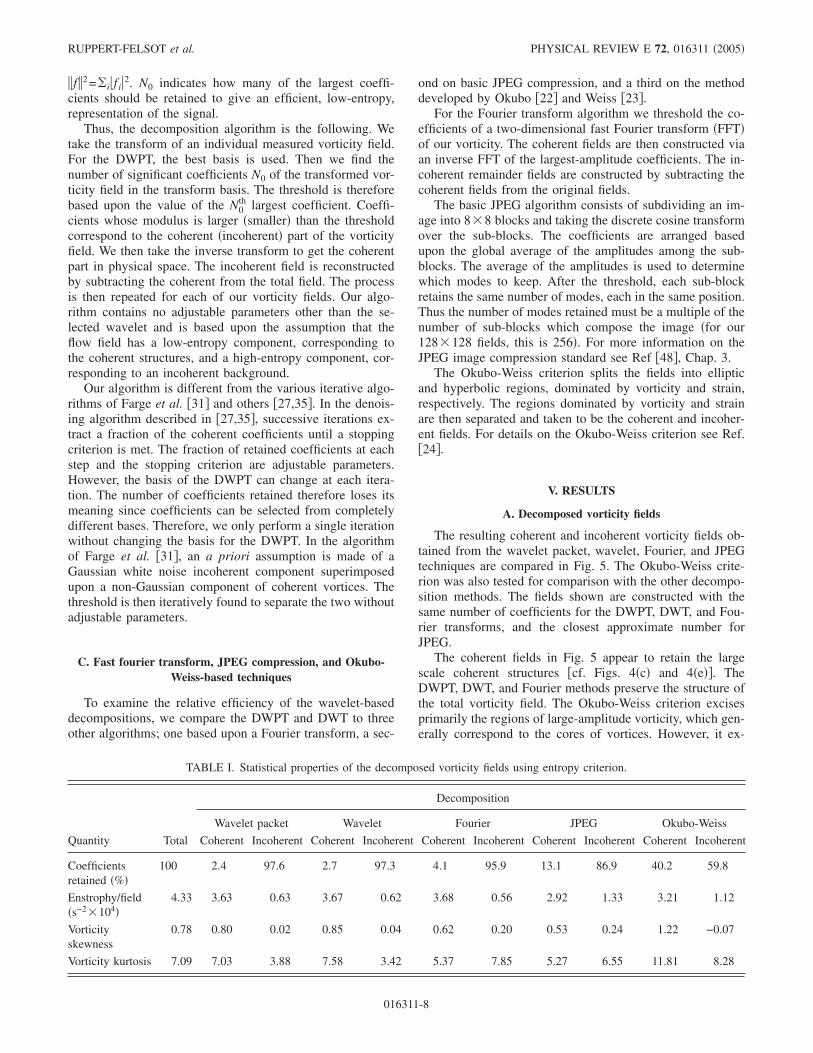
TABLE I. Statistical properties of the decomposed vorticity fields using entropy criterion.

Quantity Total

Decomposition

Wavelet packet Wavelet Fourier JPEG Okubo-Weiss

Coherent Incoherent Coherent Incoherent Coherent Incoherent Coherent Incoherent Coherent Incoherent

Coefficientsretained �%�

100 2.4 97.6 2.7 97.3 4.1 95.9 13.1 86.9 40.2 59.8

Enstrophy/field�s−2�104�

4.33 3.63 0.63 3.67 0.62 3.68 0.56 2.92 1.33 3.21 1.12

Vorticityskewness

0.78 0.80 0.02 0.85 0.04 0.62 0.20 0.53 0.24 1.22 −0.07

Vorticity kurtosis 7.09 7.03 3.88 7.58 3.42 5.37 7.85 5.27 6.55 11.81 8.28


016311-8

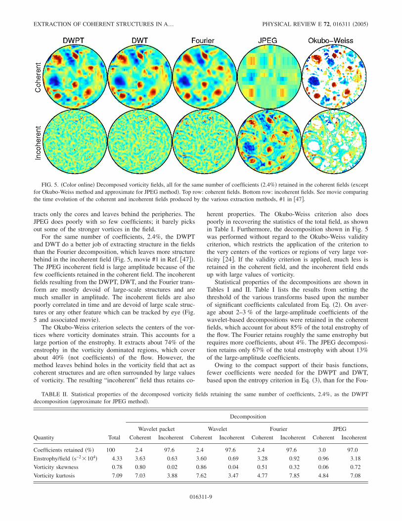
tracts only the cores and leaves behind the peripheries. TheJPEG does poorly with so few coefficients; it barely picksout some of the stronger vortices in the field.

For the same number of coefficients, 2.4%, the DWPTand DWT do a better job of extracting structure in the fieldsthan the Fourier decomposition, which leaves more structurebehind in the incoherent field �Fig. 5, movie #1 in Ref. �47��.The JPEG incoherent field is large amplitude because of thefew coefficients retained in the coherent field. The incoherentfields resulting from the DWPT, DWT, and the Fourier trans-form are mostly devoid of large-scale structures and aremuch smaller in amplitude. The incoherent fields are alsopoorly correlated in time and are devoid of large scale struc-tures or any other feature which can be tracked by eye �Fig.5 and associated movie�.

The Okubo-Weiss criterion selects the centers of the vor-tices where vorticity dominates strain. This accounts for alarge portion of the enstrophy. It extracts about 74% of theenstrophy in the vorticity dominated regions, which coverabout 40% �not coefficients� of the flow. However, themethod leaves behind holes in the vorticity field that act ascoherent structures and are often surrounded by large valuesof vorticity. The resulting “incoherent” field thus retains co-

herent properties. The Okubo-Weiss criterion also doespoorly in recovering the statistics of the total field, as shownin Table I. Furthermore, the decomposition shown in Fig. 5was performed without regard to the Okubo-Weiss validitycriterion, which restricts the application of the criterion tothe very centers of the vortices or regions of very large vor-ticity �24�. If the validity criterion is applied, much less isretained in the coherent field, and the incoherent field endsup with large values of vorticity.

Statistical properties of the decompositions are shown inTables I and II. Table I lists the results from setting thethreshold of the various transforms based upon the numberof significant coefficients calculated from Eq. �2�. On aver-age about 2–3 % of the large-amplitude coefficients of thewavelet-based decompositions were retained in the coherentfields, which account for about 85% of the total enstrophy ofthe flow. The Fourier retains roughly the same enstrophy butrequires more coefficients, about 4%. The JPEG decomposi-tion retains only 67% of the total enstrophy with about 13%of the large-amplitude coefficients.

Owing to the compact support of their basis functions,fewer coefficients were needed for the DWPT and DWT,based upon the entropy criterion in Eq. �3�, than for the Fou-

FIG. 5. �Color online� Decomposed vorticity fields, all for the same number of coefficients �2.4%� retained in the coherent fields �exceptfor Okubo-Weiss method and approximate for JPEG method�. Top row: coherent fields. Bottom row: incoherent fields. See movie comparingthe time evolution of the coherent and incoherent fields produced by the various extraction methods, #1 in �47�.

TABLE II. Statistical properties of the decomposed vorticity fields retaining the same number of coefficients, 2.4%, as the DWPTdecomposition �approximate for JPEG method�.

Quantity Total

Decomposition

Wavelet packet Wavelet Fourier JPEG

Coherent Incoherent Coherent Incoherent Coherent Incoherent Coherent Incoherent

Coefficients retained �%� 100 2.4 97.6 2.4 97.6 2.4 97.6 3.0 97.0

Enstrophy/field �s−2�104� 4.33 3.63 0.63 3.60 0.69 3.28 0.92 0.96 3.18

Vorticity skewness 0.78 0.80 0.02 0.86 0.04 0.51 0.32 0.06 0.72

Vorticity kurtosis 7.09 7.03 3.88 7.62 3.47 4.77 7.85 4.84 7.08


016311-9

rier and JPEG decompositions. Compression curves for theenstrophy of the various decompositions applied to our vor-ticity fields are shown in Fig. 6. The DWPT and DWT bothdo similarly well at extracting the enstrophy in the fieldswith only a small number of coefficients. The DWPT prob-ably does slightly better due to the adaptability of its basis.The Fourier-based methods do not converge as rapidly as thewavelet-based methods. This is likely due to the nonlocalityof the basis functions when applied to a field which haslocalized structures and sharp features.

The wavelet-based algorithms also do a better job pre-serving the skewness and kurtosis of the total vorticity in thecoherent component, while the incoherent components aremuch closer to a Gaussian distribution �skewness 0, kurtosis3�. Table II displays the results from setting the threshold onthe transforms so that each method retains 2.4% of the coef-ficients in the coherent component �since the JPEG coeffi-cients must be a multiple of the number of 8�8 blocks, 256,this restriction is relaxed�. For the same number of retainedcoefficients, the DWT and DWPT clearly outperform theFourier method in terms of preserving the statistics of thetotal vorticity field.

Figure 7 shows that the coherent fields from the waveletpacket and wavelet decompositions rapidly converge to thestatistics of the total vorticity field. The coherent fields pre-serve the non-Gaussianity of the vorticity probability distri-bution function �PDF� without having to extract many coef-ficients. The respective incoherent fields also rapidlyconverge to Gaussian statistics. This suggests that waveletsand wavelet packets do a good job of extracting the coherentstructures from the vorticity field. The near-Gaussianity ofthe incoherent field suggest that the transforms have left theremainder without coherent structure.

The coherent components of the Fourier and JPEG de-compositions, however, converge to the statistics of the totalfields much more slowly. To obtain the same level of fidelity,both the Fourier and JPEG decomposition must extract many

more coefficients. This inefficiency results in overtrans-formed fields. Further, the insets in Fig. 7�b� show that thekurtosis of the incoherent component never converges toanything small, but increasingly deviates from Gaussian.This suggests that the Fourier decomposition is not separat-ing the coherent structures from the background.

The probability distribution function of vorticity hasbroad wings �Fig. 8�, which correspond to the large vorticityvalues that occur in the coherent vortices and vorticity fila-

FIG. 6. �Color online� The percent enstrophy retained in thelargest-amplitude coefficients as a function of the number of coef-ficients kept. In order from best �most efficient� to worst: waveletpacket, wavelet, Fourier, JPEG results.

FIG. 7. �Color online� Convergence of the skewness and kurto-sis of the vorticity PDFs for the various decompositions, plottedwith quantities defined so that they approach unity as they con-verge. The vertical line indicates the fraction of coefficients retainedin the wavelet packet decomposition. �a� Convergence of the coher-ent component. Plotted: kurtosis ratio kcoh/ktotal; skewness ratioscoh/stotal. �b� Convergence of the incoherent component. Plotted:kurtosis ratio 2−kincoh/3; skewness ratio 1− sincoh/stotal. Note thatunity on the graph represents the respective statistic for a Gaussiandistribution: skewness 0, kurtosis 3. The kurtosis of the Fourier andJPEG incoherent fields is large and off the main plot. The insetsshow the convergence behavior at large numbers of retained coef-ficients. The open circles on the curves correspond to the fraction ofcoefficients retained for the corresponding techniques using the en-tropy criterion as a threshold.


016311-10

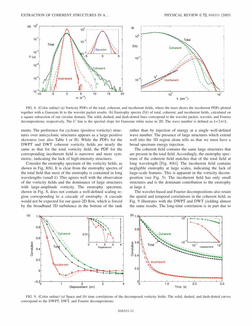
ments. The preference for cyclonic �positive vorticity� struc-tures over anticyclonic structures appears as a large positiveskewness �see also Table I or II�. While the PDFs for theDWPT and DWT coherent vorticity fields are nearly thesame as that for the total vorticity field, the PDF for thecorresponding incoherent field is narrower and more sym-metric, indicating the lack of high-intensity structures.

Consider the enstrophy spectrum of the vorticity fields, asshown in Fig. 8�b�. It is clear from the enstrophy spectra ofthe total field that most of the enstrophy is contained in longwavelengths �small k�. This agrees well with the observationof the vorticity fields and the dominance of large structureswith large-amplitude vorticity. The enstrophy spectrum,shown in Fig. 8, does not contain a well-defined scaling re-gion corresponding to a cascade of enstrophy. A cascadewould not be expected for our quasi-2D flow, which is forcedby the broadband 3D turbulence in the bottom of the tank

rather than by injection of energy at a single well-definedwave number. The presence of large structures which extendwell into the 3D region alone tells us that we must have abroad spectrum energy injection.

The coherent field contains the same large structures thatare present in the total field. Accordingly, the enstrophy spec-trum of the coherent field matches that of the total field atlong wavelength �Fig. 8�b��. The incoherent field containsnegligible enstrophy at large scales, indicating the lack oflarge-scale features. This is apparent in the vorticity decom-position �see Fig. 5�. The incoherent field has only smallstructures and is the dominant contribution to the enstrophyat large k.

The wavelet-based and Fourier decompositions also retainthe spatial and temporal correlations in the coherent field, asFig. 9 illustrates with the DWPT and DWT yielding almostthe same results. The long-time correlation is in part due to

FIG. 9. �Color online� �a� Space and �b� time correlations of the decomposed vorticity fields. The solid, dashed, and dash-dotted curvescorrespond to the DWPT, DWT, and Fourier decompositions.

FIG. 8. �Color online� �a� Vorticity PDFs of the total, coherent, and incoherent fields, where the inset shows the incoherent PDFs plottedtogether with a Gaussian fit to the wavelet packet results. �b� Enstrophy spectra Z�k� of total, coherent, and incoherent fields, calculated ona square subsection of our circular domain. The solid, dashed, and dash-dotted lines correspond to the wavelet packet, wavelet, and Fourierdecompositions, respectively. The k1 line is the spectral slope for Gaussian white noise in 2D. The wave number is defined as k=2 /L.


016311-11

the presence of long-lived coherent structures. In contrast,for the incoherent field the spatial and temporal correlationsare short ranged, indicating the absence of large-scale andlong-lived structures.

B. Transport of passive scalar particlesand concentration fields

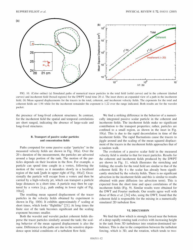
Paths computed for some passive scalar “particles” in themeasured velocity fields are shown in Fig. 10�a�. Over the20 s duration of the measurement, the particles are advectedaround a large portion of the tank. The motion of the par-ticles depends on their location in the flow. For example, aparticle can spend time caught in a vortex, following themotion of the vortex as it meanders slowly in a localizedregion of the tank �path in upper right of Fig. 10�a��. Occa-sionally the particle will escape from a vortex and then becarried by a high-velocity jet, which can transport a particlelarge distances in a short time. A particle may then be cap-tured by a vortex �e.g., path ending in lower right of Fig.10�a��.

The resulting mean squared displacement of the tracerparticles in the velocity fields obtained by experiment isshown in Fig. 10�b�. It exhibits approximately t2 scaling atshort times, which looks “flightlike” �21�. At long times thefinite size of the tank becomes significant and the scalingexponent becomes smaller.

Both the wavelet and wavelet packet coherent fields dis-perse the tracer particles similarly around the tank; the scal-ing behavior of the mean squared displacement is also thesame. Differences in the paths are due to the sensitive depen-dence upon initial conditions of a turbulent flow field.

We find a striking difference in the behavior of a numeri-cally integrated passive scalar particle in the coherent andincoherent fields. The incoherent fields make no significantcontribution to the transport properties; rather, particles areconfined to a small region, as shown in the inset in Fig.10�a�. This is due to the rapid decorrelation in time of theincoherent fields. The rapid fluctuations cause the tracers tojiggle around and the scaling of the mean squared displace-ment of the tracers in the incoherent fields approaches that ofa random walk.

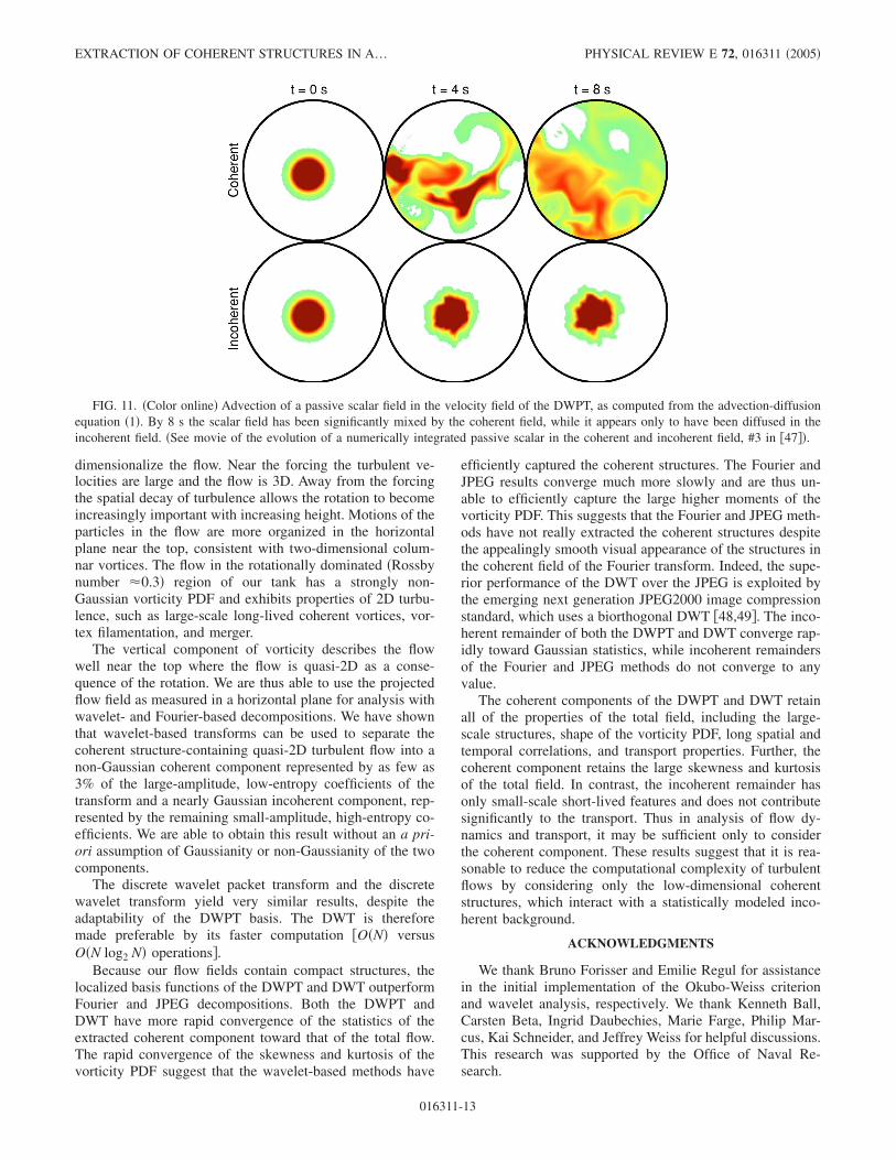
The evolution of a passive scalar field in the measuredvelocity field is similar to that for tracer particles. Results forthe coherent and incoherent fields produced by the DWPTare shown in Fig. 11, which illustrates the stretching andfolding; the results for the total field are similar to that of thecoherent field. By 4 s the scalar has already been signifi-cantly stretched by the velocity fields. There is no significantadvection in the incoherent fields and this is similar to resultsobtained with pure diffusion �no advection term�. This isexpected from the short time and space correlations of theincoherent fields �Fig. 9�. Similar results were obtained forthe DWT and Fourier methods. Our results agree well withthose of Beta et al. �34� who, using the DWT, found that thecoherent field is responsible for the mixing in a numericallysimulated 2D turbulent flow.

VI. DISCUSSION

We find that flow which is strongly forced near the bottomof a deep rapidly rotating tank evolves with increasing heightin the tank from 3D turbulence into rotation-dominated tur-bulence. This is due to the competition between the turbulentforcing, which is 3D, and the rotation, which tends to two-

FIG. 10. �Color online� �a� Simulated paths of numerical tracer particles in the total field �solid curves� and in the coherent �dashedcurves� and incoherent field �boxed regions� for the DWPT �total time 20 s�. The inset shows an expanded view of a path in the incoherentfield. �b� Mean squared displacements for the tracers in the total, coherent, and incoherent velocity fields. The exponents for the total andcoherent fields are 1.94 while for the incoherent remainder the exponent is 1.22 over the range indicated. Both results are for the waveletpacket.


016311-12

dimensionalize the flow. Near the forcing the turbulent ve-locities are large and the flow is 3D. Away from the forcingthe spatial decay of turbulence allows the rotation to becomeincreasingly important with increasing height. Motions of theparticles in the flow are more organized in the horizontalplane near the top, consistent with two-dimensional colum-nar vortices. The flow in the rotationally dominated �Rossbynumber �0.3� region of our tank has a strongly non-Gaussian vorticity PDF and exhibits properties of 2D turbu-lence, such as large-scale long-lived coherent vortices, vor-tex filamentation, and merger.

The vertical component of vorticity describes the flowwell near the top where the flow is quasi-2D as a conse-quence of the rotation. We are thus able to use the projectedflow field as measured in a horizontal plane for analysis withwavelet- and Fourier-based decompositions. We have shownthat wavelet-based transforms can be used to separate thecoherent structure-containing quasi-2D turbulent flow into anon-Gaussian coherent component represented by as few as3% of the large-amplitude, low-entropy coefficients of thetransform and a nearly Gaussian incoherent component, rep-resented by the remaining small-amplitude, high-entropy co-efficients. We are able to obtain this result without an a pri-ori assumption of Gaussianity or non-Gaussianity of the twocomponents.

The discrete wavelet packet transform and the discretewavelet transform yield very similar results, despite theadaptability of the DWPT basis. The DWT is thereforemade preferable by its faster computation �O�N� versusO�N log2 N� operations�.

Because our flow fields contain compact structures, thelocalized basis functions of the DWPT and DWT outperformFourier and JPEG decompositions. Both the DWPT andDWT have more rapid convergence of the statistics of theextracted coherent component toward that of the total flow.The rapid convergence of the skewness and kurtosis of thevorticity PDF suggest that the wavelet-based methods have

efficiently captured the coherent structures. The Fourier andJPEG results converge much more slowly and are thus un-able to efficiently capture the large higher moments of thevorticity PDF. This suggests that the Fourier and JPEG meth-ods have not really extracted the coherent structures despitethe appealingly smooth visual appearance of the structures inthe coherent field of the Fourier transform. Indeed, the supe-rior performance of the DWT over the JPEG is exploited bythe emerging next generation JPEG2000 image compressionstandard, which uses a biorthogonal DWT �48,49�. The inco-herent remainder of both the DWPT and DWT converge rap-idly toward Gaussian statistics, while incoherent remaindersof the Fourier and JPEG methods do not converge to anyvalue.

The coherent components of the DWPT and DWT retainall of the properties of the total field, including the large-scale structures, shape of the vorticity PDF, long spatial andtemporal correlations, and transport properties. Further, thecoherent component retains the large skewness and kurtosisof the total field. In contrast, the incoherent remainder hasonly small-scale short-lived features and does not contributesignificantly to the transport. Thus in analysis of flow dy-namics and transport, it may be sufficient only to considerthe coherent component. These results suggest that it is rea-sonable to reduce the computational complexity of turbulentflows by considering only the low-dimensional coherentstructures, which interact with a statistically modeled inco-herent background.

ACKNOWLEDGMENTS

We thank Bruno Forisser and Emilie Regul for assistancein the initial implementation of the Okubo-Weiss criterionand wavelet analysis, respectively. We thank Kenneth Ball,Carsten Beta, Ingrid Daubechies, Marie Farge, Philip Mar-cus, Kai Schneider, and Jeffrey Weiss for helpful discussions.This research was supported by the Office of Naval Re-search.

FIG. 11. �Color online� Advection of a passive scalar field in the velocity field of the DWPT, as computed from the advection-diffusionequation �1�. By 8 s the scalar field has been significantly mixed by the coherent field, while it appears only to have been diffused in theincoherent field. �See movie of the evolution of a numerically integrated passive scalar in the coherent and incoherent field, #3 in �47��.


016311-13

�1� A. K. M. F. Hussain, J. Fluid Mech. 173, 303 �1986�.�2� K. R. Sreenivasan, Rev. Mod. Phys. 71, S383 �1999�.�3� S. K. Robinson, Annu. Rev. Fluid Mech. 23, 601 �1991�.�4� J. C. R. Hunt, Annu. Rev. Fluid Mech. 23, 1 �1991�.�5� J. T. C. Liu, Annu. Rev. Fluid Mech. 21, 285 �1989�.�6� J. Lumley and P. Blossy, Annu. Rev. Fluid Mech. 30, 311

�1998�.�7� J. Sommeria, S. D. Meyers, and H. L. Swinney, Nature

�London� 331, 689 �1988�.�8� J. C. McWilliams, J. Fluid Mech. 146, 21 �1984�.�9� NOAA/NESDIS interactive GOES archive, available at http://

wist.ngdc.noaa.gov/wist/goes.html�10� http://visibleearth.nasa.gov/�11� A. D. McEwan, Nature �London� 260, 126 �1976�.�12� A. Colin de Verdiere, Geophys. Astrophys. Fluid Dyn. 15, 213

�1980�.�13� E. J. Hopfinger, F. K. Browand, and Y. Gagne, J. Fluid Mech.

125, 505 �1982�.�14� S. C. Dickinson and R. R. Long, J. Fluid Mech. 126, 315

�1983�.�15� R. H. Kraichnan, Phys. Fluids 10, 1417 �1967�.�16� L. M. Smith, J. R. Chasnov, and F. Waleffe, Phys. Rev. Lett.

77, 2467 �1996�.�17� L. M. Smith and F. Waleffe, Phys. Fluids 11, 1608 �1999�.�18� F. S. Godeferd and L. Lollini, J. Fluid Mech. 393, 257 �1999�.�19� J. Paret and P. Tabeling, Phys. Rev. Lett. 79, 4162 �1997�.�20� A. Provenzale, Annu. Rev. Fluid Mech. 31, 55 �1999�.�21� T. H. Solomon, E. R. Weeks, and H. L. Swinney, Phys. Rev.

Lett. 71, 3975 �1993�.�22� A. Okubo, Deep-Sea Res. Oceanogr. Abstr. 17, 445 �1970�.�23� J. Weiss, Physica D 48, 273 �1991�.�24� C. Basdevant and T. Philipovitch, Physica D 73, 17 �1994�.�25� P. Holmes, J. L. Lumley, and G. Berkooz, Turbulence, Coher-

ent Structure, Dynamical Systems and Symmetry �CambridgeUniversity Press, New York, 1996�, Chap. 3.

�26� I. Daubechies, Ten Lectures on Wavelets �SIAM, Philadelphia,1992�.

�27� A. Siegel and J. B. Weiss, Phys. Fluids 9, 1988 �1997�.�28� C. Schram and M. L. Riethmuller, Meas. Sci. Technol. 12,

1413 �2001�.�29� M. Farge, Annu. Rev. Fluid Mech. 24, 395 �1992�.�30� M. Farge, E. Goirand, Y. Meyer, F. Pascal, and M. V. Wicker-

hauser, Fluid Dyn. Res. 10, 229 �1992�.�31� M. Farge, K. Schneider, and N. Kevlahan, Phys. Fluids 11,

2187 �1999�.�32� M. Farge, http://wavelets.ens.fr/�33� M. Farge, K. Schneider, G. Pellegrino, A. A. Wray, and R. S.

Rogallo, Phys. Fluids 15, 2886 �2003�.�34� C. Beta, K. Schneider, M. Farge, and H. Bockhorn, Chem.

Eng. Sci. 58, 1463 �2003�.�35� M. V. Wickerhauser, Adapted Wavelet Analysis from Theory to

Software �A. K. Peters, Wellesley, MA, 1994�.�36� A. K. M. F. Hussain, Phys. Fluids 26, 2816 �1983�.�37� J. E. Ruppert-Felsot, MS thesis, The University of Texas at

Austin, 2003.�38� M. Raffel, C. Willert, and J. Kompenhans, Particle Image Ve-

locimetry: A Practical Guide �Springer-Verlag, Berlin, 1998�.�39� E. E. Michaelides, J. Fluids Eng. 119, 233 �1997�.�40� A. M. Fincham and G. R. Spedding, Exp. Fluids 23, 449

�1997�.�41� A. Fincham and G. Delerce, Exp. Fluids 29, S13 �2000�.�42� K. Okamoto, S. Nishio, T. Saga, and T. Kobayashi, Meas. Sci.

Technol. 11, 685 �2000�. This work describes image genera-tion for PIV and CIV algorithm evaluation;http://piv.vsj.or.jp/piv/

�43� A. K. Prasad, Exp. Fluids 29, 103 �2000�.�44� J. Pedlosky, Geophysical Fluid Dynamics, 2nd ed. �Springer-

Verlag, New York, 1987�.�45� W. H. Press, B. P. Flannery, S. A. Teukolsky, and W. T. Vet-

terling, Numerical Recipes in C: The Art of Scientific Comput-ing �Cambridge University Press, New York, 1988�.

�46� L. N. Trefethen, Spectral Methods in Matlab �SIAM, Philadel-phia, 2000�.

�47� See EPAPS Document No. E-PLEEE8-71-103504 for the aux-iliary materials. A direct link to this document may be found inthe online article’s HTML reference section. The documentmay also be reached via the EPAPS homepage �http://www.aip.org/pubservs/epaps.html� or from ftp.aip.org in thedirectory /epaps/. See the EPAPS homepage for more informa-tion.

�48� T. Acharya and P.-S. Tsai, JPEG 2000 Standard for ImageCompression �Wiley-Interscience, Hoboken, NJ, 2005�.

�49� http://jpeg.org/jpeg2000/index.html


016311-14

extraction of coherent structures in a rotating turbulent...

Documents