numerical simulation on wind flow over step-shaped cliff ... · pdf fileinfluence on the...

Int. J. Environ. Res., 7(1):173-186, Winter 2013ISSN: 1735-6865

Received 20 April 2012; Revised 4 Aug. 2012; Accepted 17 Aug. 2012

*Corresponding author E-mail: [email protected]

173

Numerical Simulation on Wind Flow over Step-shaped Cliff Topographywith Rough Surface

Yassin, M.F.1,2*and Al-Harbi, M.1

1 Department of Environmental Technology Management, Kuwait University, Kuwait2 Faculty of Engineering, Assiut University, Egypt

ABSTRACT:To enhance the understanding of the impact of obstacle buildings on pollution transportationand dispersion in the atmospheric boundary layer, it is necessary to know the atmospheric flow characteristicsover terrains. Wind flow characteristics in a boundary layer over a step-shaped cliff topography model withrough and smooth surfaces were studied numerically using Computational Fluid Dynamics models (CFD).The CFD models that were used for the simulation were based on the steady-state Reynolds-Average Navier-Stoke equations (RANS) with turbulence models; standard and RNG models. The rough surface was modeledusing windbreak fence, which was set on the step-shaped cliff model surface. The results of the numericalmodel were validated against the wind tunnel results in order to optimize the turbulence model. Numericalpredictions agreed reasonably with the wind tunnel results. The results indicated that rough surface has a greatinfluence on the turbulent flow characteristics and vortex rotating. The wind velocity for rough surface near theground level was observed to be lower than that for the smooth surface of the step-shaped cliff model. Largeflow separations were formed by the windbreak fences. Distortion of the flow at the windward corner of thestep created a steep gradient of velocity and large turbulent mixing.

Key words: Atmospheric turbulence,CFD models, Rough surface,Terrain model,Wind flow

INTRODUCTIONWind flow above complex terrain has become one

of the most important topics of environmental research.This is because wind turbines are increasingly erectedin areas with complex orography, furthering the courseof wind energy is the main impetus for the investigation.Good knowledge of the flow over complex terrain isessential for precisely estimating wind energy potential,assessing structural loads on turbines. Anunderstanding of flow in complex terrain is also crucialfor the parameterization of form drag in meteorologicalmodels. It is also significant for various dispersionapplications. Several studies have paid a great deal ofattention to atmospheric boundary layer flow over hills.Jackson and Hunt (1975) presented their two-dimensional (2D) analysis of turbulent flow in complexterrain, which was later extended to three-dimensional(3D) flow by Mason and Stykes (1979). This theory hasbeen refined and implemented numerically intocommercial codes such as MS3DJH, MSFD and WAsP(Taylor et al. 1983; Walmsley et al. 1986; and Beljaars etal. 1987). These so-called linear models have theadvantage of producing computationally fast and

accurate results for terrains of gentle slopes of lessthan 0.3 or 17æ% (Wood 1995; Walmsley and Taylor1996).Until recently, many investigators haveattempted to measure turbulence in the backward-facing step flow with sophisticated experimentaltechniques (Eaton and Johnston, 1981). However, thereare relatively fewer studies on wind flow over step-shaped topography with turbulent boundary layer(Bowen and Lindley, 1977; Adams and Johnston, 1988;Friedrich and Arnal, 1990; Djilali and Gartshora, 1991;Kasagi and Matsunaga, 1993; Olsson, 1999). Williamand Joseph (2000) evaluated the viability of using astep-shaped terrain representation of a smoothmountain profile in model simulations of small-amplitude mountain waves, where the result can becompared against known analytic solutions. Ross etal. (2004) have performed numerical and experimentalstudies in order to assess the performance of differentturbulence closure schemes in predicting the flow fieldover a hill. Two-dimensional steep hills of differentslopes, in both neutral and stably stratified flowconditions were studied. Loureiro and Freire (2005)have investigated the effects that a large change in

174

Yassin, M.F. and Al-Harbi, M.

surface elevation provokes on the properties of theatmospheric using wind tunnel and water channelexperiments. Mouzakis and Bergels (2005) presentpredictions of the two-dimensional turbulent flow overa triangular ridge. Turbulent boundary layer with a stepchange in surface roughness was investigatedexperimentally by Krogstad and Nickels (2006). Poggiaet al. (2007) collected a new data set above a terrain ofgentle hills to explore experimentally and theoreticallythe 2-D structure of the mean velocity. Blocken et al.(2007) addressed the problem of horizontalhomogeneity associated with the use of sand-grainroughness wall functions. This is done by focusingon the CFD simulation of a neutrally stratified,horizontally homogeneous atmospheric boundary layerflow over uniformly rough, flat terrain.

This paper presents the results of numericalinvestigatation for studying the effect of the roughsurface on the wind flow in the turbulent boundarylayer over step-shaped cliff topography. Therefore, theaim of the present work is to improve the understandingof mechanism of simulation on the wind flow overterrain topography and to predict the wind flow overlocal topography. For this purpose, a two-dimensionalmodel of step-shaped cliff with and without obstaclesfence was considered. Mean velocity, turbulenceintensity and turbulent kinetic energy were analyzedand discussed at different locations in the downwinddistance over step-shaped cliff model under neutralatmospheric conditions.

MATERIALS & METHODSIn this paper, the numerical simulations were

performed using the FLUENT CFD code (Fluent, 2009),which is based on the finite volume method to solvethe equations of conservation for the differenttransported quantities in the atmospheric flow (mass,momentum and energy). The code first performs thecoupled resolution of the pressure and velocity fieldsand then evolution of other parameters.

A two-dimensional step-shaped cliff configurationwas chosen as a model of steep curvature obstacles.The model geometry is shown in Fig. 1. In this figure,Z‘ means the height from the upper surface of the step-shaped cliff. The step-shaped cliff model is modeledon a 1:1000 scale. The geometry chosen was identicalto that examined experimentally in a wind tunnel study

by Yassin et al. (2001), where the cliff height was 75 mhigh in the real scale and its length was 20H (H=75mm). The simulated rough surface was modeled withwindbreak fence and the simulated smooth surfacemodeled without windbreak fence. The windbreakfence was set on the step-shaped cliff model surface.The computational domain was 3 m long x 1.8 m high,which was discretised as 109 x 50 grids. The modeledge distance 7H from the inlet domain, 13.33H fromthe outlet domain, and 29.33H from the upper domain.Extensive tests of the grid intervals are carried out withincreasing grid interval until further refinement is shownto be less significant. The computational meshemployed was a conventional non-uniform mesh, forwhich the optimal mesh was identified, consisting of634675 cells of average side sizes. The origin of thedomain was defined at the center of the front edge ofthe step-shaped cliff model. The expansion ratio in thenon-uniform grid was 1.1. The grid intervals near theobstacles in the x-, and z-directions are ∆x =0.16H, and∆z = 0.12H respectively. Fine cells were defined overthe step-shaped cliff model, where high gradients wereexpected, and coarse cells elsewhere. A meshrefinement test was performed to identify the optimalmesh resolution and ensure the results were mesh-independent. To minimize truncation error, cell-sizeincrements were gradual and limited to a maximumincrement of 25% between contiguous cells. In Fluent,The grid was generated using GAMBIT software. Thecomputational grid configurations over the step-shaped cliff model with and without obstacle fence areshown in Fig. 2.

The FLUENT CFD package has been configuredto solve the Navier Stokes equations for the flow overthe step-shaped cliff using the standard k-ε turbulencemodel (Launder and Spalding, 1974) and RNG k-εturbulence model (Yakhot et al., 1992) for computationalefficiency and accuracy. The RNG k-ε model differsfrom the standard k-ε turbulence scheme only throughthe modification to the equation for ε, which includesan additional sink term in the turbulence dissipationequation to account for non-equilibrium strain ratesand employs different values for the model coefficients(Kim and Baik, 2004). The governing equations of themodel are shown belowContinuity equation

0=∂∂

i

i

xu (1)

Momentum equation

⎪⎭

⎪⎬⎫

⎪⎩

⎪⎨⎧

′′−⎟⎟⎠

⎞⎜⎜⎝

⎛

∂

∂+

∂∂

∂∂

+∂∂

−=∂∂

+∂∂

jii

j

j

i

jiij

j

i uuxu

xu

xxpuu

xtu ν

ρ1)( (2)

Int. J. Environ. Res., 7(1):173-186, Winter 2013

175

Smooth surface Rough surface

Fig. 2. the computational step-cliff configuration

143.0ZUα Z ′

Z

H

X X/H=0

UH

Z’=0

Fig. 1. Two-dimensional step-cliff model

Tke - transport equation

ενσν

−∂∂

⎟⎟⎠

⎞⎜⎜⎝

⎛

∂

∂+

∂∂

+⎟⎟⎠

⎞⎜⎜⎝

⎛∂∂

∂∂

=∂∂

+∂∂

j

i

i

j

j

it

ik

t

ii

i

xu

xu

xu

xK

xxKu

tK

(3)

ε - transport equation for standard k-ε turbulence model

Kc

xu

xu

xu

Kc

xxxu

t j

i

i

j

j

it

i

t

ii

i2

21ενεε

σνεε

εεε

−∂∂

⎟⎟⎠

⎞⎜⎜⎝

⎛

∂

∂+

∂∂

+⎟⎟⎠

⎞⎜⎜⎝

⎛

∂∂

∂∂

=∂∂

+∂∂

(4)

ε - transport equation for RNG k-ε turbulence model

RK

cxu

xu

xu

Kc

xxxu

t j

i

i

j

j

itls

i

t

ii

i −−∂

∂⎟⎟⎠

⎞⎜⎜⎝

⎛

∂

∂+

∂

∂+⎟⎟

⎠

⎞⎜⎜⎝

⎛

∂∂

∂∂

=∂

∂+

∂∂ 2

2ενεε

σνεε

εε

(5)

)1(/1

30

023

ηβηηεηµ +

−=

kcR (6)

2/1

⎪⎭

⎪⎬⎫

⎪⎩

⎪⎨⎧

∂∂

⎟⎟⎠

⎞⎜⎜⎝

⎛

∂

∂+

∂∂

=j

i

i

j

j

i

xu

xu

xuK

εη (7)

iji

j

j

itji K

xu

xuuu δν

32

−⎟⎟⎠

⎞⎜⎜⎝

⎛

∂

∂+

∂∂

=′′− (8)

εν µ

2K

ct =(9)

176

Numerical Simulation on Wind Flow

where, ui is the ith mean velocity component; p isthe deviation of pressure from its reference value andρ is the air density. νt is the turbulent viscosities ofmomentum, respectively, δij is the kronecker delta. ν isthe kinematic viscosity of air. η =4.38 and β0 = 0.012.Table 1 show the constant values in the transportequations.

In modeling atmospheric flow, smaller grid size isdesirable near the surface of the step-shaped cliffmodel to better resolve flow, but away from the model,a larger grid size is allowable. The governing equationsset was solved numerically on a staggered grid systemusing the finite-volume following the semi-ImplicitMethod for pressure-Linked Equation (SIMPLE)algorithm described by Patankar (1980). The standardand RNG k-ε turbulence models were employed herefor comparison because of its widespread acceptancein diverse fields.

Velocity inlet boundary layer conditions were usedin the main inlet wind flow. The initial wind speed isuniform (10 m/s) with low turbulence intensity. A user-defined subroutine for including the turbulence 0.143the power law in rural area inlet velocity profile intoFLUENT code was developed and used in the analysis.The initial condition for wind velocities, turbulentkinetic energy, K and its dissipation rate ε are specifiedas (FLUENT, 2009)

where, UH is the velocity at a height ZH ; Z is theheight above the ground, and n is the power exponent,uτ is the friction velocity and l is the turbulence lengthscale. The ground and step-shaped cliff surfaces aredefined as walls with no-slip boundary condition. Thewall boundary conditions for momentum are applied toall solid surface and rough walls. Zero gradientboundary conditions are applied at the outflow andupper boundaries.

The experimental data was used for the validationof numerical simulation obtained from a detailed windtunnel study by Yassin et al. (2001). Experiments wereperformed in a closed-circle boundary layer wind

n

HH Z

ZUU ⎟⎟⎠

⎞⎜⎜⎝

⎛= (11)

µ

τ

cuK

2

= (12)

lTc Ke )(

2/34/3

µε = (13)

tunnel, which is shown in Fig.3. The width and heightof the test section were 2.2 and 1.5 m. A neutral stratifiedatmospheric boundary layer was simulated using threespires, one 90 mm high cubic array placed justdownstream of the contraction exit and followed by 60and 30 mm cubic roughness element, covering 10.2 mof the test-section floor. This arrangement wasemployed to generate a thick turbulent boundary layeras the approaching flow. Reynolds number based onUH and H is 3.5 x 104. Fig. 4 shows the simulatedturbulent boundary layer profile at X=0.0 correspondsto the center of the step model. Tripping wires (1 mmrectangular columns, 50 mm intervals) were arrangedover the step-shaped cliff. The windbreak fence overthe step-shaped cliff was a solid plate fence, and waspositioned at intervals of 50 mm, the same as for thetripping wires.

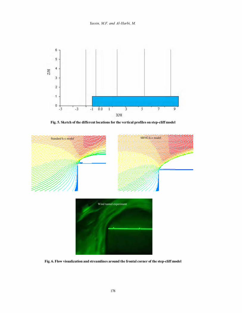
Wind velocity was measured using a hot wireConstant Temperature Anemometer (CTA) system witha split fiber probe, which was 70 µm diameter and 1.25mm long. This was because the X-wire probeanemometers for turbulence measurement cannot givereasonable accuracy when the turbulence intensity islarger than 0.3 (Ishihara, 1999). Wind velocitymeasurements over the step-shaped model were madewith split-fiber probe (55R55) in conjunction with a90N10 DANTEC constant temperature anemometersystem. The mean velocity was normalized by thereference velocity, UH which is the velocity of the step-shaped cliff height. The velocity profiles weremeasured at the positions over the step-shaped cliffsurface shown in Fig. 5. To clarify the change in theflow characteristics, the simulated data wereinterpolated at the same grid points as in the windtunnel experiment. Smoke flow visualization was donein the wind tunnel to see what kind of flowcharacteristics appeared around the windward cornerand over the step-shaped cliff model. The numericalresults of the wind tunnel experiments for the flowstructure were compared using the flow visualizationand streamlines around the windward corner and overthe step-shaped cliff model, as is shown in Fig 6. Onthe windward corner of the step-shaped cliff, the flowseparation was created. A reattachment point appearedover the step-shaped cliff and moved downstreamtowards the downwind street. The numerical simulationof the wind flow was therefore consistent and inagreement with the measurements used in wind tunnelexperiments.The simulated data was interpolated at thesame grid points as in the wind tunnel experiment. Thenumerical data of the standard and RNG k-ε turbulencemodels was validated against the data obtained fromthe wind tunnel experiments at various locations. Figs.7-8 show the vertical profiles of the normalizedhorizontal velocity for the surfaces with and without

177


1800 mm

Wind

1450 mm

Roughness

Roughness Roughness

Step-c liff model

Split -Fiber probe

10215 mm

Spires

H=75mm

Z Y

X

Wind

6550 mm 2215 mm 1256 mm

Roughness Roughness Roughness

Split -

Spires Z Y

X

90x90x90 mm 60x60x60 mm 30x30x30 mm

Fig. 3. Schematic diagram of the wind tunnel experimental

1

10

100

1000

1 10 100

0.01 0.1 1 Turbulence intensity

Mean velocity

m/s

Z, mm

Fig. 4. Vertical distribution of mean velocity and turbulence intensity of incident flow (at X= -800 mm & Y=0)

obstacles fence at X/H=-5, -1, 0.5, 3.8, 7.8 and 11.8. Agood agreement between the turbulence models andthe wind tunnel experiment was observed for both thesurfaces without and with obstacles fence. A slightdifference between the turbulence models and the windtunnel experiments for the surface without obstaclesfence was observed at X/H=-5, 7.8 and 11.8 and for thesurface with obstacles fence at X/H=-5, and 0.5, whichcould have been due to the use of three-dimensionalisolated step-shaped cliff in the wind tunnel experiment.However, the standard turbulence model was showedto be generally close to the wind tunnel experimentsfor the surface without obstacles fence.

RESULTS & DISCUSSIONSThe distributions, vectors, and streamlines of the

horizontal velocity over the step-shaped cliff modelfor the rough and smooth surfaces are shown in Figs9-11. Fig.12 shows the vertical profiles of the meanhorizontal velocity over the step-shaped cliff modelfor the rough and smooth surfaces without at variouslocations; X/H=-5, -1, 0.5, 3.8, 7.8 and 11.8.

These figures show that the standard and RNGturbulence model predict similar wind velocities overthe step-shaped cliff model, except for the smoothsurface at 1<Z/H<1.75. The most intensive movement

Table 1. Constants in the turbulence models

Models c µ c1 ε c2ε σk σ ε standard κ-ε model 0.09 1.44 1.92 1.0 1.3

RNG κ-ε model 0.085 1.42 1.68 0.7179 0.7179

178


Fig. 5. Sketch of the different locations for the vertical profiles on step-cliff model

Standard k-ε model SRNG k-ε model

Wind tunnel experiment

Fig. 6. Flow visualization and streamlines around the frontal corner of the step-cliff model

179


Fig. 7 .Vertical profiles of normalized horizontal velocity over step-cliff model without windbreak fence atdifferent locations X/H

Fig. 8. Vertical profiles of normalized horizontal velocity over step-cliff model with windbreak fence atdifferent locations X/H

180


Standard k-ε model Without windbreak fence

m/s RNG k-ε model Without windbreak fence

m/s

Standard k-ε model With windbreak fence

m/s RNG k-ε model With windbreak fence

m/s

Fig. 9. Mean horizontal velocity distributions over the step-cliff model

Standard k-ε model Without windbreak fence

Standard k-ε model With windbreak fence

RNG k-ε model Without windbreak fence

RNG k-ε model With windbreak fence

Fig. 10. Mean horizontal velocity vectors over the step-cliff model

181


Fig. 11. Streamlines of the mean horizontal velocity over the step-cliff model

Fig. 12. Vertical profiles of normalized horizontal velocity over step-cliff model at different locations

182


of the flow appeared near the windward corner of thestep-shaped cliff. The mean horizontal velocityappeared to be very small at the windward corner ofthe step-shaped cliff. The vortex appeared to berotating clockwise on the step-shaped cliff roughsurface between every windbreak fences and for thesmooth surface near the ground windward of the step-shaped cliff. The vortex was generated by standardturbulence model was observed smaller than that byRNG turbulence model. A negative velocity was foundfor the surface with obstacles fence. This meant thatthe air movement associated with the vortex-likemotion effectively towards both the leeward andwindward of the windbreak fences in the step-shapedcliff. The wind velocity adjacent for the smooth surfacewas higher than that for the rough surface of the step-shaped cliff. Flow separation at the windward cornerof the step-shaped cliff for the smooth surface wasquite small if present at all, and compared to the roughsurfaces. Relatively large flow separations were formedby the windbreak fences. The difference between thesmooth and rough surfaces was relatively small at Z/H>2. A thick internal boundary layer was generated bythe rough surface. Inversely, internal boundary layerfor the smooth surface was very thin because therewas no windbreak fence. While, at X/H= 0.5, the thickinternal boundary layer was generated over the smoothsurface compared to the other due to the turbulentmixing, which was formed by the distortion of flow atthe windward corner of the step-shaped cliff. Themaximum velocity was observed at X/H= 0.5 for thesmooth and rough surfaces. This was because thewindward corner generated the separation flow. Theprevious results showed that the rough surface has agreat influence on the flow characteristics and vortexrotating.

Besides the mean velocity, it is of interest to knowhow turbulence might be modified as the flow goesover the step-shaped cliff model. Turbulence structuresbehind two-dimensional hill are poorly understood.Figs13-14 show the contours of the turbulence intensityover the step-shaped cliff model for the smooth andrough surfaces. The vertical profiles of the turbulenceintensity over the step-shaped cliff model for thesmooth and rough surfaces at various locations; X/H=-5, -1, 0.5, 3.8, 7.8 and 11.8 are shown in Fig.14.Vigorous turbulent mixing was observed in the upperpart of the frontal corner of the step-shaped cliff model.The turbulence intensity over the rough surfaceappeared to have similar patterns at Z/H<2. While, theturbulence intensity over the smooth surface appearedto have similar patterns on the step-shaped cliff surfaceat X/H=3.8, 7.8 and 11.8 for Z/H<2 respectively. Theturbulence intensity varied slowly with height. Over

the step-shaped cliff, there was significant highintensity near the surface and this led to a large increasein the turbulent stress. There was a strong gradient inthe turbulence intensity at X/H=0.5 with the maximummagnitude close to the step-shaped cliff surface. Aregion of high-turbulence intensity appeared to bealong the shear layer downstream of the step-shapedcliff model. Peak values of the turbulence intensitycreated in the zones were characterized by the highestvelocity gradients. The turbulence intensity showedhigher value at Z/H<2 over the step-shaped cliff forthe smooth surface due to the steep gradient of thevelocity than that of the rough surface. The value ofthe turbulence intensity over the step-shaped cliff atX/H= 3.8, 7.8 and 11.8 for the rough surface was largerthan that for the smooth surface.

The turbulent kinetic energy is one of the mostimportant variables in the atmospheric boundary layer.Figs. 15-16 show the contours and vertical profiles ofthe turbulent kinetic energy over the step-shaped cliffmodel for the smooth and rough surface surfaces. It isshowed that an increase in wind velocity significantlydecreases the turbulent kinetic energy over the step-shaped cliff model. The distribution of the turbulentkinetic energy quantifies the turbulent diffusion alongthe shear layer and is consistent with the direction ofthe mean flow. The turbulent energy for the rough andsmooth surfaces had similar pattern at Z/H>2. The peakvalue of the turbulent energy appeared to be near thewindward corner at X/H=0.5 for the surface withoutobstacles fence and was considered to be closelyrelated to the small separation as described above. Theminimum value of the turbulent energy for the surfacewithout an obstacle fence was displayed at X/H=-5.The values of turbulent energy appeared to be slightlyhigher at Z/H<2 for the rough surface than that for thesmooth surface, except at X/H=0.5 due to the largevelocity gradient.

CONCLUSIONA two-dimensional computational fluid dynamics

(CFD) model with the standard and RNG k-ε turbulencemodels were used to investigate the effects of thesmooth and rough surfaces on the atmospheric flowover two-dimensional step-shaped cliff model usingFLUENT code. The validation of the numerical modelwas evaluated and agreed with wind tunnel data. Thevalidation of the numerical simulation through the windtunnel experiment enhances the aspect that numericalsimulations, which are a low-cost tool able to providein reasonable time accurate results regarding fluiddynamics problems. The current study clearly indicatesthat there is significant influence of the smooth and

Standard k-ε model Without obstacle fence

Standard k-ε model With obstacle fence



Fig. 13. Turbulence intensity distributions over the step-cliff model

Fig. 14. Vertical profiles of normalized turbulence intensity over step-cliff model at different locations


183


RNG k-ε model Without obstacle fence


RNG k-ε model With obstacle fence

Fig. 15. Turbulent kinetic energy, K distributions over the step-cliff model

Fig. 16. Vertical profiles of normalized turbulent kinetic energy, K over step-cliff model atdifferent locations


184

185


rough surfaces on the wind flow over the step-shapedcliff model, the following conclusions can be made: (a) For mean velocity field, the most intensivemovement of the flow appeared near the windwardcorner of the step-shaped cliff. The mean horizontalvelocity appeared to be very small at the windwardcorner of the step-shaped cliff. The vortex appearedto be rotating clockwise on the step-shaped cliffsurface for the rough surface between every windbreakfences and for the smooth surface near the groundwindward of the step-shaped cliff. Inverse flow wasfound with the rough surface. The wind velocityadjacent to the smooth surface was higher than thatof the rough surface of the step-shaped cliff. A thickinternal boundary layer was generated by theobstacles fence.

(b) For turbulent field, vigorous turbulent mixingwas observed in the upper part of the frontal cornerof the step-shaped cliff model. The turbulenceintensity varied slowly with height. A region of high-turbulence intensity appeared to be along the shearlayer downstream of the step-shaped cliff surface.Peak values of the turbulence intensity created in thezones were characterized by the highest velocitygradients. The turbulence intensity showed highervalue at Z/H<2 in the step-shaped cliff for the smoothsurface. An increase in wind velocity significantlydecreases the turbulent kinetic energy over the step-shaped cliff model. The distribution of the turbulentkinetic energy quantifies the turbulent diffusionalong the shear layer and is consistent with thedirection of the mean flow. The peak value of theturbulent energy appeared to be near the windwardcorner at X/H=0.5 for the smooth surface. Theminimum value of the turbulent energy for the smoothsurface was displayed at X/H=-5.

REFERENCESAdams, E. W. and Johnston, J. P. (1988). Effects of theSeparating Shear Layer on the Reattachment Flow Structure.Exp. Fluids, 6, 493-499.

Beljaars, A., Walmsley, J. and Taylor, P. (1987). A mixedspectral finite difference model for neutrally stratifiedboundary layer flow over roughness changes and topography.Boundary-Layer Meteorol., 38, 273–303.

Blocken, B., Stathopoulos, T. and Carmeliet, J. (2007). CFDsimulation of the atmospheric boundary layer: wall functionproblems. Atmospheric Environment 41, 238-252.

Bowen, A. J., and Lindley, D. (1977). A Wind TunnelInvestigation of the Wind Speed and TurbulenceCharacteristics Close to the Ground over Various Escarpmentshapes. Boundary Layer Meteorology, 12, 259-271.

Djilali, N. and Gartshora, I. S. (1991). Turbulent Flowaround a Bluff Rectangular Plate. Part 1: ExperimentalInvestigational. J. of Fluid Engineering, Trans. of ASME,113 (3), 51-59.

Eaton, J. K. and Johnston, J. P. (1981). A Review ofResearch on Subsonic Turbulent Flow Reattachment. AIAAJournal, 19 (9), 1093-1100.

FLUENT Inc. (2010). FLUENT 6.3.16 user Manual.

Friedrich, R. and Arnal, M. (1990). Analyzing turbulentbackward-facing steep flow with lowpass-filtered navier-stokes equations. Journal of Wind Engineering and IndustrialAerodynamics, 35, 101-128.

Ishihara, T., Hibi, K. and Oikawa, S. (1999). A wind tunnelstudy of turbulent flow over a three-dimensional steep hill.J. of Wind Eng. and Indus. Aerodyn., 83, 95-107.

Jackson, P, and Hunt, J. (1975). Turbulent wind flow over alow hill. Q J Roy Meteorol Soc., 101, 929–955.

Kasagi, N. and Matsunaga, A. (1993). Turbulencemeasurement in a separated and reattaching flow over abackward-facing step with the aid of three-dimensionalparticle tracking velocimetry. Journal of Wind Engineeringand Industrial Aerodynamics, 46, 821-829.

Krogstad, P. A. and Nickels, T. B. (2006). Turbulentboundary layer with a step change in surface roughness.13th International Conference on Fluid Flow Technologies,6-9 September 2006, Budapest, Hungary.

Launder, B. E. and Spalding, D. E. (1974). The numericalcomputation of turbulent flows. Comp. Meth. Appl. Mech.Eng., 3, 269-289.

Loureiro, J. B. R. and Silva Freire A. P. (2005). ExperimentalInvestigation of Turbulent Boundary Layers over SteepTwo-dimensional Elevations. J. of the Braz. Soc. of Mech.Sci. & Eng., 27 (4), 329-344.

Mason, P. and Stykes, R. (1979). Flow over an isolated hillof moderate slope. Q J Roy Meteorol Soc., 105, 383–395.

Olsson, L. (1999). Steps towards an environmentallysustainable transport system. The Science of the TotalEnvironment, 235, 407-409.

Patankar, S. V. (1980). Numerical heat transfer and fluidflow. McGraw-Hill.

Poggia, D. Katulb, G., Albertsonc, J. D and Ridolfid, L.(2007). An experimental investigation of turbulent flowsover a hilly surface. Physics of Fluids, 19 (3), 036601-036612.

Ross, A. N., Arnold, S., Vosper, S. B., Mobbs, S. D., Nixon,N. and Robins, A. G. (2004). A comparison of wind-tunnelexperiments and numerical simulations of neutral andstratified flow over a hill. Boundary Layer Meteorology,113, 427-459.

Taylor, P.A., Walmsley, J. and Salmon, J. (1983). A simplemodel of neutrally stratiûed boundary-layer ûow over realterrain incorporating wave number-dependent scaling.Boundary-Layer Meteorol., 26, 169–189.


186

Walmsley, J. and Taylor, P. (1996). Boundary-layer flowover topography: impacts of the Askervein study. BoundaryLayer Meteorol., 78, 291–320.

Walmsley, J., Taylor, P. and Keith, T. (1986). A simple modelof neutrally stratified boundary layer flow over complexterrain with surface roughness modulations . Boundary LayerMeteorol., 36, 157–186.

William, A. G. and Joseph, B. K. (2000). Behavior of flowover step topography, American Meteorological Society.April, 1153-1164.

Wood, N. (1995). The onset of separation in neutral,turbulent flow over hills. Boundary Layer Meteorol., 76,137–164.

Yassin, M. F., Kato, S., Ooka, R., Murakami, S., Takahashi,T. and Ohtsu, T. (2001). Wind tunnel study on predictionof wind characteristic over local topography for suitablesite of wind power station (part 3): turbulent characteristicsof flow over a two dimensional step model. Summaries oftechnical papers of annual meeting, AIJ.

numerical simulation on wind flow over step-shaped cliff ... · pdf fileinfluence on the...

Documents