external imbalances and growth - uv · external imbalances and growth mariam camarero university...
TRANSCRIPT
External imbalances and growth
Mariam Camarero
University Jaume I and INTECO
Jesús Peiró-Palomino
University Jaume I and INTECO
Cecilio Tamarit
University of València and INTECO
Abstract
The purpose of the paper is to investigate the role that unbalanced net foreign asset
positions play in the growth path of the economies. In particular, the hypothesis to be
tested is whether external imbalances may constrain growth in debtor countries. We
analyze a large sample of countries using Lane and Milesi-Ferretti “External Wealth of
Nations Dataset” and employing both parametric and nonparametric techniques. We
find a preponderant positive relationship between the external position and growth,
although the impact differ between countries and temporal periods.
Keywords: Economic growth; net external position; nonparametric regression
Communications to: Jesús Peiró-Palomino, Department of Economics, University Jaume
I, Campus del Riu Sec, 12071 Castelló de la Plana, Spain. Tel: +34 964728592, Fax: +34
964728591, e-mail: peiroj�uji.es

1. Introduction and motivation
The analysis of the impact of high levels of external indebtedness on economic growth
has mostly been confined up to now to developing countries. However, after years of
global and large external imbalances, somewhat adjusted and mitigated during the re-
cent financial crisis, the evolution of imbalances and their prospective effects on future
growth remains a matter of concern for both, developed and developing countries, also
in times of recovery. For those countries that suffered large imbalances in the eve of the
crisis, the question is whether this can be a constraint for recovery and long-run growth
prospects. Blanchard et al. (2015) have emphasized that after the crisis, output growth may
have slowed down, calling for the concepts of hysteresis or super-hysteresis coined by Ball
(2014). The rational behind this reasoning is that high levels of external leverage may divert
resources from investment and other productive uses to service the debt, reducing growth
in the long-run and leading to a Secular Stagnation process.
The theoretical literature has distinguished between the positive short-run effects of
accumulating external imbalances in order to finance investment and the negative long-run
growth effects of high levels of indebtedness. The underlying idea is that the impact of the
net external indebtedness on growth is sensitive to the debt level itself. Theoretical works
suggest, in fact, a non-linear relationship and the existence of an optimal level of debt,
giving rise to an external debt Laffer curve,1 although the supporting empirical evidence is
mixed.2 This study analyses the impact of the net external position on growth for a wide
range of developed and developing nations. We use data from the Penn World Tables
and the last update of the Lane and Milesi-Ferretti (2001) database, covering the period
1983–2011. The net foreign assets (NFA) relative to GDP is used as a measure of the net
external position.3 The value of assets owned by domestic residents held abroad (A) minus
the value of domestic liabilities to the rest of the world (L) is called the national NFA or
1The relationship between net external position and growth has been focus of much work historically.There exists a set of theoretical models predicting inverted U-shaped curves. The growth rate increases withindebtedness until a given threshold, after which growth reduces. The underlying idea is that when thethreshold is passed, the economy moves to another regime, with the indebtedness-growth nexus being differentfrom the old one. In the inverted “U” models, the low-indebtedness regime corresponds to an increasingindebtedness-growth relationship, while in the regime after the threshold the indebtedness-growth relationshipis decreasing.
2Different strategies have been implemented in the empirical literature to estimate the externalindebtedness-growth relationship, leading to a wide variety of results across countries (see Pattillo et al., 2011,for a recent review of the literature).
3The choice of this variable for the analysis is widely discussed in Section 3.2.
1

external wealth of a nation. A country, therefore, can be a net creditor (NFA > 0), or a net
debtor (NFA < 0).
The increasing degree of economic and financial integration led by the globalization
process since the 80’s has affected expenditure decisions for two reasons. First, the sig-
nificant improvement in the conditions of access to external financing, and second, the
prospects for future improvements in productivity that may have induced agents to over-
shoot on their spending decisions.4 These overly optimistic expectations may have led
to unsustainable current account deficits and capital movements with puzzling allocative
results and destabilizing financial effects raising the frequency and severity of economic
crises. Consequently, this paper also relates to a recent strand of the literature analyzing
the effects of financial globalization (see, for instance, Prasad et al., 2007; Ayhan Kose et al.,
2009; Obstfeld, 2009).
Kraay and Ventura (2000, 2002) and Ventura (2003) showed that although for indus-
trial countries the classic intertemporal models (IA) perform well empirically, neither the
IA nor the Real Business Cycle (RBC) models are appropriate for the emerging market
countries. Therefore, a new class of models emphasizing the role of strategic default on
foreign debts (also called sovereign risk) was developed (see Aguiar and Amador, 2014).
More recently, Broner and Ventura (2016) have made a pathbreaking contribution to ex-
plain the pattern of capital flows and their macroeconomic consequences. They show how
the sovereign’s behavior worsens as a result of globalization, emphasizing the role of mi-
croeconomic frictions in financial markets. If these frictions are present, wealth plays a
role as collateral when borrowing, so that autarky interest rates might be lower in capital-
scarce countries than in capital-abundant ones even if the marginal product of capital is
higher. This prediction, contrary to the IA models, helps to solve the allocation puzzle coined
by Gourinchas and Jeanne (2013) and to explain why capital flows towards rich countries
with developed financial markets. Puzzles, however, are not constrained to developing
countries. The recent financial and economic crisis of 2008-09 has raised serious concerns
about the long-term sustainability of external imbalances where sovereigns’ position are
subject to multiple equilibria driven not only by fundamentals but by variations in market
sentiments.4The dynamics of the external accounts are explained by agents’ response to transitory and permanent
shocks, in particular shocks in productivity. In the case of favorable productivity or technological shocks, likethe expectations triggered by the creation of the euro, investment booms tend to enhance output growth butworsen the external accounts (Glick and Rogoff, 1995).
2

In this context, this paper aims to address not only the role of net external positions on
growth, but also attempts to unravel how the process of globalization might influence this
relationship. We follow Broner and Ventura (2016) trying to identify different behaviors
for countries sharing similar relative positions (creditor or debtor), geographical location
or particular country-specific characteristics such as the stage of development (GDP per
capita), institutional quality, financial development or commercial openness. In contrast
to previous contributions, which mostly rely on parametric estimations, we apply non-
parametric kernel regressions (see Li and Racine, 2007; Henderson and Parmeter, 2015).
Empirical contributions in the field of economic growth using these techniques are on the
rise (see, for instance Henderson et al., 2012b, 2013), 5 since they are data-driven methods
providing a flexible framework and allowing for nonlinearities. In addition, they provide
observation-specific estimates, so that parameter heterogeneity in both the spatial and the
temporal dimension can be easily exploited.
The remainder of the paper is organized as follows: Section 2 reviews the previous
theoretical and empirical literature on the external imbalances-growth nexus, starting from
the neoclassical growth model up to more recent theories that explain some paradoxical
stylized facts related to external imbalances; in Section 3 we account for the empirical
methodology, whereas the main empirical results are presented in Section 4. Finally, Sec-
tion 5 concludes.
2. Theoretical review and related empirical literature
From a theoretical point of view, the neoclassical growth model has been considered the
standard workhorse framework for the analysis of financial integration and its conse-
quences. In this model, capital moves from countries with low autarky returns to those
with high autarky returns.6 Moreover, each country’s autarky returns are determined by
two factors: capital abundance/scarcity and growth prospects in the long-run. The long-
term external position of a country would depend on the gap between the world interest
rate and its autarky rate, but will be also proportional to the difference between the world’s
and its own productivity. Also, the rate of growth of consumption per capita is equal to the
5GDP per capita growth has been explained by a large number of theories. It is common practice toconsider the Solow variables as the baseline model, where variables from other theories such as demography,policy, geography, fractionalisation, institutions or financial development are added (see Henderson et al., 2012b,2013, for recent examples using nonparametric methods in this context).
6See Gourinchas and Rey (2014) for a detailed description of the main elements of the model.
3

world’s growth rate of productivity (independently of the country’s productivity growth).
The main prediction of this theory is that advanced economies will have low autarky re-
turns, and emerging countries would be the ones with high rates. Thus, capital flows would
go from rich to poor countries. That means that countries export capital when this factor
is relatively abundant, in a similar fashion as the principles of comparative advantage.
The fulfillment of the neoclassical theory would imply a negative relationship between
growth and the net foreign position of a country: this means that creditor countries would
reduce their growth rate whereas debtor countries will increase their growth thanks to
the contribution of external resources. Moreover, according to this, the most advanced
economies would grow at a lower rate than less affluent countries leading to a catching-up
process.
Empirical evidence, however, not always supports the neoclassical theory. In particular,
important stylized facts of the international capital markets are difficult to be reconciled
with these predictions. For example, the US has been importing capital since 1982, coming
from emerging economies (Stylized Fact 1 in (Gourinchas and Rey, 2014)). Moreover, pro-
ductivity growth and net capital inflows are not always positively related–i.e. the so-called
“allocation puzzle” (Gourinchas and Jeanne, 2013)–commonly explained by the effect of
the public capital flows. Alternatively, an important consequence that could be derived
from these facts is that rich countries may have, in reality, higher productivity (otherwise
they would not attract private capital). Thus, they would accumulate capital inflows and
diverge from emerging countries, widening the income gap with them. However, the em-
pirical evidence suggests that emerging countries have higher productivity growth and, at
the same time, are accumulating capital outflows.
Before the recent eurozone crisis, the evolution of peripheral European countries was
considered evidence in favor of the neoclassical theory. However, later on it was shown
that those countries (i. e. Spain) had instead very low productivity growth and that the
large inflow of capital was more related to the financing of the residential housing boom
than to productive investment.7
Newer theories or extensions of the neoclassical model have tried to explain these puz-
zling facts and the pattern of external imbalances.8 Their underpinnings were laid out
by the maximizing models that took over the field of international economics in the early
7Portugal constitutes a similar example, as described in Blanchard (2007).8For a survey on the literature about the relationship between financial development and economic growth
see Levine (2005).
4

1980s. According to Broner and Ventura (2016) their purpose was to explain the pattern
of capital flows and their macroeconomic consequences from two competing sources: the
intertemporal approach (IA) to the current account and the open-economy versions of the
Real Business Cycle (RBC).9 Although the IA models tend to show a quite high explanatory
power for the case of developed economies, neither the IA nor the RBC seem to perform
well empirically in the case of developing countries, and therefore the causal mechanisms
behind borrowing and growth remain imperfectly understood. Gourinchas and Rey (2014)
describe extensively the most relevant explanations trying to fill this gap. Asymmetries in
financial development (among countries at different stages of economic development) may
explain international imbalances due to demographic differences or asset shortage (limited
domestically acceptable collateral). In particular, according to Ferrero (2010) population ag-
ing, increasing savings, lower autarky interest rates, and therefore, countries with rapidly
aging populations (such as Germany or Japan) run external surpluses. In addition, idiosyn-
cratic risk triggers precautionary savings as argued by Aiyagari (1994), so that additional
demand for savings further reduces domestic interest rates. Another possible explanation
is provided by Antràs and Caballero (2009) and Jin (2012) who analyze the links between
trade flows and capital flows. Specialization (in labour or capital intensive products) may
determine that a country becomes capital exporter or importer. Finally, valuation effects
have been very large recently and have acted through the financial channel of external
imbalances, as found by Gourinchas and Rey (2007).10
With this aim, Gourinchas and Rey (2007) decomposed the external adjustment into a
financial (valuation) channel and a trade (net export) channel and show that the deteriora-
tion in net exports or net foreign asset positions of a country have to be matched either by
future net export growth (trade adjustment channel) or by future increases in the returns of
net foreign asset portfolio (financial adjustment channel). The valuation channel is impor-
tant in the medium-term, whereas the net export channel is more relevant in a long-time
horizon. While temporary current account deficits may simply reflect the reallocation of
capital to countries where capital is more productive, persistent deficits may be regarded
9See Obstfeld and Rogoff (1996) and Blanchard et al. (2016) for a description of both models.10In contrast to the traditional trade channel, we can assess the nature and dimension of external imbalances
by looking at the NFA position of countries. The negative values of the NFA position reflect the cumulatedeffect of persistent current account deficits, and therefore, the imbalance between foreign assets and liabilities.However, a country running persistent current account deficits might be at the same time improving its NFAposition if capital gains on its foreign assets exceed those on its foreign liabilities (Lane and Milesi-Ferretti,2007). With valuation effects, the changes in the NFA position do not coincide with the current account. Thismay explain some of the imbalances but it is hard to incorporate in the theoretical models.
5

as a more serious issue. Deficits may lead to increased domestic interest rates to attract
foreign capital. However, the accumulation of external debt due to persistent deficits may
imply increasing interest payments that impose an excess burden on future generations.
The current account plays the role of a buffer against transitory shocks in supply (pro-
ductivity) or demand (government spending, or interest rates, among others) in order to
smooth the inter-temporally optimal consumption path. However, in the long-run, the no-
Ponzi game restriction, which is regarded as synonymous with the fulfillment of the Inter
temporal External Budget Constraint (IEBC) that all countries face, requires that today’s
external debt is matched by an excess of future primary surpluses over deficits in present
value terms. All nations are subject to a budget constraint that requires that the value of
gross domestic expenditure (GDE) or absorption, plus the change in the stock of foreign
assets owned by domestic residents (At − At−1) equals the value of gross domestic product
(GDP) plus the change in the stock of domestic debt owed to foreigners (Lt − Lt−1). Com-
bining this relationship with the definition of the current account, it follows that the change
in the NFA position is the same as the balance on the current account. Therefore, if the
current account is in deficit (CA < 0), the change in the NFA is negative, indicating that
the increase in foreign debt was greater than the increase in foreign assets over the year. A
negative change in the NFA is referred to as a net capital inflow, since more capital flowed
into the country through additions to the level of foreign debt than flowed out through
purchases of foreign assets.
Let us consider a stochastic setting, in which the economy is characterized by an en-
dogenous policy response to the balance of payments or a borrowing constraint that main-
tains external debt at some constant optimal ratio to income (n f a∗) pursuing a growth
maximizing leverage strategy (Fleming and Stein, 2004). Dividing by the level of GDP and
imposing the foreign debt sustainability condition that the ratio of NFA to GDP be constant
at a given level n f a∗, we find that the critical net current account position to GDP ratio,
ca∗, is:
ca∗t = (g − i)n f a∗, (1)
where g is the growth rate of nominal GDP and i is the real interest rate.
Therefore, exports (imports) respond positively (negatively) to debt in excess of the
optimal ratio. In practical terms, the arithmetic of solvency examines whether the net
6

debt/GDP ratio grows more or less rapidly than the difference between the real interest
rate and the economy’s growth rate. To sum up, this equation signals a clear relationship
between the net level of external debt and the growth rate of the economy.
Debt overhang may induce a poorer macroeconomic policy environment (i.e. less in-
centive to undertake difficult structural reforms) as it generates expectations of debt re-
structuring and/or uncertainty about other ways of financing with distortionary effects
on the efficiency of the system (inflation tax or cuts in productive public investment).
Also, in resource-rich countries, spending resource revenues domestically may lead to
Dutch disease, hurting the competitiveness of traded good sectors and, hence, growth
(e.g., Van der Ploeg (2011) and Van der Ploeg and Venables (2013)). History reveals that,
during windfalls, resource-rich countries that plan to increase public investment together
with external borrowing may bear substantial debt risks. As stated in Greenlaw et al. (2013)
a strand of the literature has looked at the determinants of currency and sovereign debt
crises, much of it focusing on the experience of developing economies.11 Eichengreen et al.
(2005) described the inability of emerging market countries to borrow in their own cur-
rencies as an original sin.12 Unfortunately, the recent experience has shown that more
advanced economies are not immune to potential sovereign-debt problems similar to those
widely observed in less developed economies.13
Even in models with repudiation risk, low levels of debt are still associated with higher
growth than in financial autarky. However, beyond a certain threshold or tipping point
level of accumulated debt stock, growth can diminish due either to expected higher taxes to
service the debt or simply because future debt will be larger than the country’s repayment
ability and foreign investment is discouraged (Krugman, 1988). This new class of models
emphasizing the role of strategic default of foreign debts (also called sovereign risk) makes
the same predictions as the IA models. Strategic default reduces the size of the effects,
but it does not change their nature. Therefore, it was necessary to find more alternative
theories and the focus shifted from macroeconomic or sovereign risk to microeconomic
11Reinhart et al. (2003) found that emerging-market economies have a lower tolerance for sovereign debt,with defaults at much lower levels of debt to GDP. Reinhart and Rogoff (2010) provided further evidence.Mishkin (1996, 1999) attributed the lower debt tolerance of emerging-market economies to their weaker finan-cial institutions and greater vulnerability to international capital flows.
12The denomination of debt in foreign currencies implies that a currency depreciation increases the debtburden, which can lead to financial crises, a collapse in the economy and further exchange rate depreciation.The possibility of this vicious cycle puts limits on the amount of debt that a country can issue and constrainsmonetary policy options.
13De Grauwe (2012) argued that the periphery countries of the European Monetary Union are in a similarsituation to emerging economies, forced to borrow in a currency (the euro) whose supply they do not control.
7
frictions in financial markets. If wealth plays a role as collateral when borrowing, autarky
interest rates might be lower in capital-scarce countries than in capital-abundant ones due
to the higher risk involved in financial transactions in capital-scarce countries even if its
marginal product of capital is higher.
This fact reverses the predictions of the IA models regarding the pattern of capital flows,
so that financial liberalization can reduce investment and growth in developing capital-
scarce countries swapping risky, high-return assets for safe, low-return assets in developed
countries. This is a promising approach to explain why capital flows towards countries
that are already rich and with developed financial markets (financial depth effect). In a
recent paper, Broner and Ventura (2016) develop a model aiming at reconciling the different
stylized facts present in the literature of the effects derived from financial globalization. The
model stresses the role of imperfect enforcement of domestic debts and the interactions
between domestic and foreign debts. According to these authors the outcome in terms of
growth of the external position of a country involved in a process of financial globalization
will depend on the initial level of development together with other fundamentals, namely,
the level of productivity, domestic savings, and the quality of institutions.
Financial globalization changes the mix of creditors, raising the number of foreign hold-
ers of domestic debt and increasing the political incentive for the domestic debtors (private
and public) to default on their debt, raising the probability of a financial crisis. But the
probability of a financial crisis will depend as well on a set of additional observable coun-
try characteristics (the initial income level, domestic savings, level of productivity and the
quality of enforcement institutions) and an unobservable variable: the market sentiment or
investors expectations (optimistic or pessimistic laws of motion) about the probability of
default. Productivity, savings and the quality of institutions although they scale up the
dynamics of the process, do not change the law of motion of the model. Therefore, ceteris
paribus the effects on growth of the globalization process will depend critically on the level
of development of the country that liberalizes (threshold effects).
As Broner and Ventura (2016) show, contrary to the representative-agent benchmark
models, where financial globalizations always lead to capital inflows in developing coun-
tries, the effects of financial globalization are heterogenous. A country that liberalizes is
subject to three different possible outcomes in terms of capital flows and growth depending
on the level of development. At a low level of development, the country imports capital
and growth accelerates (the capital-flight effect is weak because domestic financial markets
8
are very shallow and globalization still results in net capital inflows). However, if financial
globalization takes place at an intermediate level of development, financial globalization
leads to net capital outflows and slows down growth (domestic capital flight effect prevails).
Finally, if financial globalization occurs at high levels of development, we are under multi-
ple equilibria: there will be capital imports and higher growth under optimist expectations
and capital exports and lower growth under pessimism giving rise to recurrent cycles of
high and low-growth periods. A seemingly successful economy might suddenly face a
shift from optimism to pessimism under a self-fulfilling expectations process that results
in a sudden stop in capital inflows, reversing into capital outflows and a reduction in in-
vestment and growth. The optimistic equilibrium only exists beyond a threshold: only in
countries that are sufficiently rich and which have deep enough domestic financial markets
the optimistic equilibrium exists and financial globalization is more likely to lead to capital
inflows and higher investment and growth (financial-depth effect). Concerning the empir-
ics, as pointed out by Checherita-Westphal and Rother (2012) the empirical literature has
focused until recently on the role of the external debt in developing countries and found
this to be a key predictor of financial crises in emerging economies.14 The estimated re-
lationships, mainly in reduced form specifications, have taken cubic or quadratic forms;
the estimation methods have also varied from OLS to panel data with fixed or random
effects, Tobit, or semi-parametric estimation; in addition, explanatory variables have also
been augmented including lagged values, population density, locational variables, micro or
macro variables, distributional variables, trade variables, as well as non-economic variables
such as literacy rates or political rights. Some of these studies find evidence of a positive
relationship between debt and growth for low borrowing levels while others find a negative
effect for a high debt level. Concerning the functional form, some authors have found that
the correlation between external debt and economic growth is linear, while others signal
to a non-linear relationship. Thus, while Schclarek (2004) claims that they have a linear
relationship, some other studies such as Pattillo et al. (2011), Smyth and Hsing (1995), and
Cohen (1997) argue that they follow a non-linear pattern.
Government deficits and current-account deficits often appear together, with the gov-
ernment effectively funding its shortfall by borrowing from abroad. The more government
debt is held by foreigners, the greater the political incentives for the government to default
on that debt. In a rational market, this would translate into a higher sovereign borrowing
14See, for instance Smyth and Hsing (1995); Cohen (1997); Pattillo et al. (2011); Clements et al. (2003);Schclarek (2004); Bussière and Fratzscher (2006); Bussière (2013).
9
cost. Alternatively, if the government borrows from domestic banks who in turn are largely
capitalized by foreign lending, the public debt may be domestically held but the political
economy could work out similarly to the case when the sovereign debt is held directly by
foreigners. Furthermore, a higher overall foreign debt load (both public and private) may
make it more difficult for a country to continue to make interest payments on its sovereign
debt. For these reasons a strand of the literature has focused on the exploration of the
relationship between the interest rate, the current account and total indebtedness.15
Cohen (1997) uses the external indebtedness as a variable representing the predicted
risk of a debt rescheduling (or debt crisis) to measure its effects on growth finding a thresh-
old of external debt to GDP of 50%. Reinhart et al. (2003) find a much lower threshold level
for some countries: 15%, while others, as Elbadawi et al. (1997) find a debt maximizing
level clearly higher: 97%. A recent strand of literature aims at ascertaining whether and
to what extent the external debt-growth nexus depends on country-specific characteristics,
such as the quality of their policies and institutions.16 Imbs and Ranciere (2005) confirm
a 60% level result using non-parametric methods. Pattillo et al. (2011) also find evidence
of a hump-shaped effect of debt overhang using regressions augmented with debt dummy
variables for the threshold between 35-40% of GDP.
The evidence available seems to suggest that the existence of high levels of external debt
for prolonged periods may have significant macroeconomic repercussions. From the theo-
retical revision above, we can single out the different mechanisms at stake that explain the
external debt-growth nexus. First, high levels of external debt are usually associated with
higher interest rates and, via crowding-out of funding for the private sector, lead to lower
medium term GDP growth rates. However, the latest evidence suggests that it is not pos-
sible to find a particular threshold of public debt valid for all the countries. Second, high
external debt levels reduce the leeway for a counter-cyclical fiscal policy, triggering auster-
ity measures and possible debt crisis episodes. Third, connected to the former mechanism,
the sustainability of a high level of external debt, in a context of moderate growth, requires
large and sustained primary current account surpluses, which may affect the potential
growth of the economy. Fourth, the effects of external indebtedness are heterogeneous
depending on the income level of the country together with other fundamental variables,
15The general findings in Gale and Orszag (2003), Reinhart and Sack (2000) are that a one-percentage-pointincrease in the actual or projected debt-to-GDP ratio raises the long rate by 3-7 basis points.
16The results are heterogeneous; see for instance Rresbitero (2008) who finds evidence of a threshold layingin a range from 10% to 30% for poor countries.
10
as productivity, domestic savings level and the quality of institutions. Finally, a high ex-
ternal debt-to-GDP ratio generates larger borrowing requirements in the short term, which
increase the economy’s vulnerability to financial market conditions.
To sum up, although both, negative and positive, relationships are compatible with the
different types of models, in order to clarify our results, we can establish the following
testing hypotheses for our empirical analysis:
1. A majority of negative relationships between NFA and growth would be evidence in
favor of the neoclassical models. According to these models, this relationship tends
to be homogeneous for all types of countries (developed or developing) but can be
subject to the existence of threshold effects (intertemporal external budget constraint)
that limit growth. Standard representative-agent based or IA (inter-temporal) mod-
els show how capital inflows affect the economy through two channels: currency
appreciations and cheaper financial intermediation, with opposite results on growth
and leading to boom-bust cycles.17 This evidence is also compatible with open RBC
models. If this negative relationship prevails, that would be signaling that debtor
countries achieve better performances in terms of growth and that external financial
liberalization should always be the right strategy (up to some threshold).
2. A majority of positive relationships between NFA and growth would mean that creditor
countries are the ones that win from external financial liberalization. In this case, the
theoretical support lies both in sovereign risk models and especially, the ones that pay
special attention to the microeconomic frictions in financial markets. Some of these
models, like Broner and Ventura (2016) combine both elements and are compatible
with heterogenous performances depending on the characteristics of the countries.
Therefore, the right policy to achieve a successful financial opening up process should
be designed accordingly on a country-specific basis.
Up to now the empirical evidence is far from being conclusive and calls for further
research. Our hypothesis is that the existence of a positive or negative relationship
between NFA and growth will depend critically on the type of the country (stages
of development) together with other fundamental characteristics like the domestic
financial market, the rate of saving, the productivity levels or the institutional qual-
ity that may affect the investor’s expectations and trigger sharp changes in financial
17The sign will depend on the nature of the capital flows, i.e. short-term vs. long-term effects.
11

flows, investment and growth. The econometric approach adopted allows us to un-
cover these elements and single out its relative importance with a high degree of
detail.
3. Empirical framework
3.1. Nonparametric kernel regressions
The external net position-growth nexus is assessed by means of nonparametric kernel re-
gressions. However, as a preliminary approach, we also run standard parametric (OLS)
estimations, which commonly take the following form:
Yit = β0 +T
∑j=1
β jZjit + ǫit, i = 1, 2, ...n, t = 1, 2, ...k (2)
where Yit is the average growth rate of GDP per capita for country i in period t, Z is a
vector of T regressors and β0 and β j are the associated parameters. ǫit is the error term,
and i and t refer to countries and time periods, respectively.
Despite offering an interesting first approach, parametric regressions have several short-
comings derived from their restrictive assumptions (for instance, the linearity of the pa-
rameters and those concerning the distribution of the error term). Alternatively, a more
flexible framework is provided by nonparametric regressions, which relax many of these
assumptions given its data-driven nature. Let us consider the nonparametric counterpart to
Equation (2), given by:
Yit = m(Zit) + ǫit, i = 1, 2, ...n, t = 1, 2, ...k (3)
where all the elements other than m(.) are equivalent to Equation (2). m(.) represents
an unknown smooth function, which captures the conditional relationship between the
dependent and the independent variables. This relationship is given by the data, and can
be linear or nonlinear.
There are different alternatives to estimate Equation (3). We employ the local-linear
least squares (LLLS) estimator, introduced by Racine and Li (2004). This estimator is based
on “generalized product kernels” and provides optimal estimations for mixed data sets
with both continuous and categorical variables.
The LLLS estimator computes a weighted least-squares regression around every sam-
12

ple point zit and neither a predefined functional form nor a distribution of the error term
are required (Li and Racine, 2007). A kernel function and a bandwidth vector establish the
weights such that more weight is given to those observations near to zit . The functional
form of m(.) can be drawn after connecting the estimated points. Let us reconsider Equa-
tion (3). Adopting a first-order Taylor expansion for the continuous variables, denoted as
zc, we obtain:
Yit ≈ m(z) + (zcit − zc)β(zc) + ǫit (4)
where β(zc) is the partial derivative of m(z) with respect to zc. The LLLS estimator of
δ(z) ≡ [m(z), β(zc)]′ is expressed as
δ̂(z) = [Z′K(z)Z]−1Z′K(z)y (5)
where Z is a n x (qc + 1) matrix with i row (1, (zcit − zc)) and K(z) is a n diagonal matrix of
product kernel weighting functions. For continuous variables the selection is the Gaussian
kernel; for ordered categorical variables the Wang and Van Ryzin (1981) kernel is chosen.
For additional details see Li and Racine (2007) and Henderson and Parmeter (2015).
As it is common in nonparametric methodologies, the essential point is not the choice
of the kernel but the selection of appropriate bandwidths, responsible for the degree of
smoothing. Among the various automated bandwidth selection procedures, we select least-
squares cross-validation (LSCV), employed in recent studies in the economic growth field
(see, for instance Henderson et al., 2012b, 2013). When using the LLLS estimator, the band-
widths not only determine the degree of smoothing, but also provide information on the
linearity of the regressors. When a bandwidth of a continuous regressor hits its upper
bound this implies that the regressor enters the model linearly. The upper bounds are de-
fined as two standard deviations for continuous variables whereas for ordered categorical
variables the upper bound is the unity (see Hall et al., 2007).
As we mentioned in the introduction, nonparametric regression provides observation-
specific estimates. In our context, this allows for the construction a posteriori of different
groups of countries and/or time periods in order to evaluate whether the effect of our
variable of interest is similar in countries sharing similar characteristics and comparable
over time.
Finally, as an additional robustness check, the adequacy of estimating nonparametric
13

regressions is assessed by computing Hsiao et al. (2007) tests. These compare the paramet-
ric and nonparametric models and establish which one is preferable given the data. Under
the null hypothesis (H0 : Pr[E(x|z) = f (z, β)] = 1) the parametric model is the correct
specification. Contrarily, if the the alternative (H1 : Pr[E(x|z) = f (z, β)] < 1) cannot be
rejected, it is preferred the nonparametric specification.
3.2. Models, variables and data sources
This section describes the models to be estimated and the data. We estimate four models.
In all of them the dependent variable is the average GDP per capita growth. Model 1 is a
simple model which only considers the external net position (net foreign assets, NFA) as
an explanatory variable. Model 2 is a neoclassical Barro-type growth equation (see Barro,
1991), considering as baseline the Solow (1957) model. It includes the initial GDP per
capita (in logs), population growth,18 investment (share of GDP) and a human capital index
(in logs).19 To that well-known growth regression framework, the external net position
is added as an additional regressor.20 Model 3 incorporates both regional and temporal
fixed effects to Model 2. Similarly to Henderson et al. (2013), which evaluates the role of
financial development on growth, we make use of the World Bank geographical country
classification to generate regional fixed effects, whereas the temporal effects are referred to
different sub-periods whose information is detailed in the next paragraph.21 Finally, Model
4 includes three additional regressors as control variables namely financial development,
trade openness and institutional quality. To measure financial development, following
18Following Mankiw et al. (1992) and posterior contributions, we add a constant equal to 0.05, which cap-tures depreciation and technological change.
19As it is common in the literature (see, for instance Badunenko and Romero-Ávila, 2013) the index is con-structed using a function that takes into account the average years of education (Barro and Lee, 2013) as wellas the returns to education (Psacharopoulos, 1994). The index is nowadays directly provided by internationaldatasets such as the Penn World Table.
20The selection of the baseline model is not an easy task. As put forth by Durlauf (2002), the typical cross-country growth regressions fail to capture all the potential growth determinants. As Durlauf and Quah (1999)and Brock and Durlauf (2001) argue, the fact that one particular theory could predict economic growth does notdiscredit other alternative theories as growth drivers, which represents the major difficulty for model selection.In practice, however, the great power of the Solow framework and Barro-type growth equations for predictinggrowth in different geographical contexts has meant it is widely used as a starting point when evaluating othertheories in growth empirics (see, for instance Durlauf et al., 2008; Henderson et al., 2012b, 2013).
21However, a model with country fixed effects is not estimated. For the time being, as argued byHenderson and Parmeter (2015), the implementation of the fixed effects estimator presents some difficultiesand the literature is still incipient. In our context, an alternative to the fixed effects estimation might be theinclusion of individual dummies but this would dramatically increase the number of regressors (there are 103countries in the sample). Therefore, following recent contributions in similar contexts (see Henderson et al.,2012b, 2013), we include regional dummies, which seems a balanced strategy.
14
Henderson et al. (2013), we consider the ratio of deposit bank assets/(deposits money +
central bank assets). Trade openness is measured as the ratio of imports plus exports
over GDP. Finally, among the wide variety of institutional quality indicators we consider
a composed indicator, constructed as the mean value of three items: corruption, law and
order and bureaucratic quality.
The choice of NFA as the variable measuring the external position (and vulnerability)
of a country is due to several reasons. First, the meticulous database provided by Lane
and Milesi-Ferretti allows us to make broad comparisons among countries with enough
time span to construct panel data sets. Second, it includes both external private and public
positions. This is important, because boundaries between public and private debt can
become blurred in a crisis and excluding external private positions is one the forms of
hidden debt even if it can be a source of financial instability (see Reinhart and Rogoff, 2014).
Third, this measure considers foreign currency-denominated positions, and therefore, the
related original sin problems as well as prospective valuation effects. Fourth, we consider
net positions which seems to be a better measure of external indebtedness than the gross
ones (Calderón et al., 2000). However, our choice of the NFA position is not absent of some
criticisms. As it has been recently claimed by Dias et al. (2014) using face (undiscounted)
value of assets can be misleading because countries can borrow at different maturities
and contractual forms (different distributions between principal and interest service).22
Another interesting alternative is to study the separate effects of the two components of
NFA: assets and liabilities.23 Related to the former point, some authors claim that financial
crisis affect not only net but gross international capital flows to and from the crisis country,
having important consequences on output (Broner et al., 2013; Janus and Riera-Crichton,
2015). Finally, concerning the use of the Net International Investment Position (NIIP) for
this analysis, the main problem is data availability, as both the span and the number of
reporting countries is very limited (Lane and Milesi-Ferretti, 2007).
Data for the external net position are taken from the last update of the database con-
structed by Lane and Milesi-Ferretti (2001), which currently provides data from the 1970’s
to 2013 for the majority of the world’s economies. The external net position is measured by
net stock of foreign assets as a share of GDP. As a stock variable, the authors have measured
22Dias et al. (2014) and Easterly (2002) provide alternative datasets with net present value (NPV) of debtdata.
23This goes beyond the objectives of this paper and it is an interesting research alternative to be addressedin future research.
15
the NFA position of each country in domestic currency as of Dec 31 and hence converted in
USD at the end-of-period exchange rate. However, the last update of the PWT covers only
until year 2011 and additional data constraints arise when including the full set of control
variables. Consequently, the final sample covers the period 1983–2011.
Data for the Solow variables and trade openness are provided by the Penn World Table
(PWT) 8.1. The information on financial development is available at the Financial Structure
Dataset (November 2013), whereas information on institutional quality is taken from the
Quality of Government Dataset (QOG) 2015. Following the standard practice in the growth
literature, we average data for different 5-year subperiods. The final sample comprises 550
observations for 103 countries.
3.3. Descriptive statistics
Table 1 provides some descriptive statistics. Special attention is paid to the NFA variable in
Figure 1, which displays a world map with the external net position of the countries in the
sample in 2007, the year before the economic crisis started in most of the world’s economies.
The map shows that there were only a reduced group of creditor countries at that time,
being the rest of the world a net debtor. The majority of the creditor countries are oil
producers (notably Norway, Saudi Arabia and Iran). Others, such as Japan and Germany,
are competitive exporters with aging population. In the case of China, the country has not
only surplus in the trade balance, but also an underdeveloped financial system, so that the
gains from growth and trade are invested abroad. The rest of the world is debtor, but only
a minority exceed the 100% threshold.
Figure 2 shows both the evolution and distribution of the NFA variable. In particular,
the panels a) and b) provide the temporal trend for particular country groups and indi-
vidual countries. In Figure 2 a) the OECD and the EU-15 countries display a very stable
evolution during the whole period, close to equilibrium or to a relatively small debtor
position. Internally the situation is different, as some of their members have had large
imbalances in both directions. Other areas show more volatility although, in general, the
net position tends to persist (either creditor or debtor). MENA countries are systematically
net creditors, beginning in the eighties, after the two oil price shocks and the discovery of
natural gas and oil reserves in North Africa. In contrast, the Latin American and Caribbean
area have both, as a whole, a debtor position. Sub-Saharian countries have also been net
debtors during a large part of the sample, but their position has reversed at the end of the
16
last decade. Graph b) portrays the evolution of some representative countries. Two of them,
Germany and China, are clearly net creditors. The US was balanced up to mid-nineties,
whereas Spain, Greece and Argentina are more volatile but have been net debtors during
most of the period. In the graph the Argentinian’s hardship with external debt is percep-
tible at the end of the eighties and the beginning of last decade, whereas the deterioration
of the Greek debt becomes evident since the euro inception.
Panel c) in Figure 2 provides violin plots for the different sub-periods.24 From the
inspection of these plots the main conclusion we might draw is that the NFA positions
showed lower variability in the last sub-periods, whereas in the first periods the dispersion
is higher.
4. Results
4.1. Parametric estimates
In this section we discuss the results obtained from the parametric OLS estimations, shown
in Table 2. Model 1 includes only the variable of interest, namely NFA. The estimated
coefficient, despite being relatively small is highly significant. Both the size and the signifi-
cance of the coefficient remain stable across the rest of model specifications, which include
as controls the typical Solow variables as well as regional and time effects. Considering the
most comprehensive Model 4, a 10% increase in the ratio of NFA/GDP generates a 0.08%
increase in GDP per capita. Thus, although the value of the parameter is relatively small,
the positive sign is the expected one.25 The Solow variables in models 2, 3 and 4 behave
as predicted by theory and are significant in all cases: initial GDP per capita is negative,
indicating that poorer regions grow faster than the relatively richer; population growth has
a negative sign, whereas investment in both physical and human capital shows positive
coefficients. Focusing on the additional control variables (Model 4), financial development
and institutional quality have the expected positive sign but are nonsignificant, whereas
24Violin plots are box-plots overlayed by a kernel density. The white bullet inside the box represents themedian value and the black box contains 50% of the observations (first and third quartiles correspond to thebottom and the top of the box, respectively). The vertical bars represent observations beyond these limits and,finally, the kernel density overlaying the boxplot displays the probability mass at the different values of therepresented variable.
25Some of the relationships predicted by the neoclassical model for factor mobility and growth may varydramatically, when we change the assumptions to imperfect competition and include the existence of frictionin different markets, so that the neoclassical model becomes a particular case of a more general one. See, forinstance, Markusen (1983) for the case of the complementarity among factor movements and commodity trade.
17
for trade openness we obtain an unexpected negative and significant sign.
We will use this last model as a benchmark for the rest of the analysis, bearing in mind
that we are imposing a linear relationship among all the variables. Therefore, if even in
these restrictive conditions we have been able to find that all the variables are significant
and the estimated coefficients remain stable once the control variables are introduced, this
might suggest that the NFA-growth link is relatively robust. Moreover, the NFA position,
which represents the country’s intertemporal balance between domestic savings and invest-
ment contributes positively to GDP per capita growth, in the same direction as physical and
human capital. However, we should bear in mind that the NFA position can be either pos-
itive or negative and the interpretation of the estimated coefficient should be careful. If the
country has a negative net position (that is, if the country is a debtor), an increase in this
position will reduce growth. When the net balance is positive (the country is a creditor),
the contribution of NFA to growth will be positive as well.
4.2. Nonparametric estimates
In this section we provide the results for the nonparametric counterparts of the models
considered in the preceding section. We have proceeded as follows: first, we have com-
puted the bandwidths via least squares cross validation (LSCV) and have estimated the
models using the local-linear least squares (LLLS) estimator; second, we have focused the
analysis more tightly on the NFA variable by considering potential heterogeneity and its
effects across particular groups of countries, individual countries and temporal periods.
Table 3 provides the upper bounds for the regressors as well as the bandwidths for the
different variables and models. We have marked in bold those bandwidths higher than
the corresponding upper bound, meaning that the variable enters the models linearly. In
general, the majority of the variables enter the models nonlinearly, with the exception of
financial development and the initial GDP in Model 4 and the variable of interest (NFA),
which enters linearly in models 2 and 4.
Table 3 also reports the results for the Hsiao et al. (2007) tests, described in Section 3.
They evaluate the appropriateness of the parametric estimations for all the models. In all
cases, the null hypothesis of parametric correct specification form is clearly rejected. The
results suggest that the relationship between GDP per capita growth and the regressors in-
cluded departs from linearity and, consequently, the adoption of a more flexible framework
where no functional form is predefined becomes an interesting alternative.
18

We now focus on the estimated coefficients. As noted throughout the paper, nonpara-
metric regression techniques allow us to compute individual estimates for each country
and temporal period. Table 4 reports quartile estimates for each regressor and model.
These coefficients represent the impact of a given regressor on economic growth assum-
ing that the rest of the variables remain constant at their median values. Wild bootstrap
standard errors are provided in parenthesis. In all cases the R2 for the nonparametric re-
gressions is considerably higher than that for the parametric counterparts. This supports
the appropriateness of the nonparametric methods, known for a very strong in-sample fit
(Henderson and Parmeter, 2015).
From the results presented in Table 4 we might draw that the estimated NFA coefficient
is significant in all four models and its size remains virtually unaltered when the different
controls are included. However, note that the variability across quartiles is sizable; for in-
stance, considering Model 4 the impact of NFA on growth can be four times higher in some
countries (third quartile) than in others (first quartile).26 Compared with the parametric es-
timations, the coefficient size in the nonparametric models is almost double for the third
quartile in comparison with the mean estimate provided by OLS and slightly lower for the
first quartile. This indicates that the parametric models are underestimating the impact
of NFA on growth in some countries and overestimating the effects in some others due to
model misspecification. For the rest of control variables we also detect some variability in
both the size and the significance of the coefficients, although the results are still highly
consistent with theory. In particular, for the variable trade openness we observe that the
third quartile is positive and significant, which is contrary to the result obtained with OLS
but more consistent with theory.
These quartile estimates are a useful first approach to analyze the effects on growth of
the different variables. Nonetheless, for a complete view of the results the computation
of kernel densities for the whole vector of estimated effects is a better choice. Figure 3
displays the density for NFA in all four models. In general, whereas the inclusion of the
Solow controls (Model 2) leads to similar results to those for Model 1 (simple model), the
inclusion of geographical and temporal dummies in Model 3 increases the variability of
the estimated parameter (the distribution is less pointed and shows longer tails). With the
inclusion of additional controls in Model 4, the estimated density becomes again tighter
and similar to Models 1 and 2. The median estimate, however, is fairly similar in all four
26We will try to identify later in the analysis the countries corresponding to each group.
19
models, thus indicating that the coefficient is stable and the estimation does not suffer
notable changes when additional variables are included in the model.
The NFA’s effect on growth is mainly positive and approximately normal. Most of the
effects are ranged in the interval (0–0.04), although higher and lower effects (some of them
negative) are also observed. Since from Figure 3 and Table 4 we do not perceive important
differences in the size of the NFA estimates across models, from now on we exclusively
focus on Model 4, the most comprehensive one including all the controls. The kernel den-
sity displays the entire distribution of estimates but it does not allow exploration of their
significance. Alternatively, 45o plots such as those proposed by Henderson et al. (2012a)
can easily deal with this shortcoming. They consist of plotting the estimated gradients
against themselves, which results in a 45o line, together with the associated 95% bootstrap
confidence bands for each estimate. Those intervals containing the value zero indicate that
the associated estimate is not significant. Figure 3 b) shows that most of the NFA estimates
(Model 4) in both the positive and the negative quadrant are significant.
Summarizing, the majority of the NFA gradients have a positive sign. Note however
that, according to the theory, both negative and positive signs are possible. Moreover, a
negative sign of the NFA parameter in the case of a debtor country (i.e. with a negative
NFA position) would have a positive impact on growth.
4.3. Nonparametric estimates for particular sample splits
In this section we explore whether the effects of NFA on growth differ for particular groups
of countries, individual countries and temporal periods. First, we analyze the results from
Model 4 for the case of some groups of countries and time periods. These results are
provided in Table 5. The estimated coefficient for NFA shows some variability between
groups of countries and periods.27
We have classified the results by country groups according to either economic or ge-
ographical links. The areas we consider are the OECD, the EU-15, MENA countries,
Sub-Saharian African countries, South-Asian countries and Latin-American and Caribbean
countries. In general the size and the significance of the estimated coefficient varies across
groups and temporal periods, showing that it is important to consider particular groups
27Note that the estimates for particular sample splits are not the result of partial regressions for these groups.Given that the nonparametric regression provides individual estimates for each observation, the models arerun in all cases for the entire sample and the groups (both in terms of countries and temporal periods) aremade a posteriori.
20
rather than generalize. Table 5 provides these results.
For instance, note that for the OECD group the coefficient was not significant during
the eighties and the nineties but becomes significant in 2003-2007 and practically doubles
during the crisis. A similar result is found for the EU-15.28 External imbalances accumu-
lated since the end of the nineties and the beginning of last decade have been significantly
offset after the crisis. However, in the international context, foreign capital has not always
been invested in highly productive sectors. In some cases current account imbalances were
due to consumption expenditure and real estate investment, notably in OECD countries,
whereas the funds had their origin in emerging countries. This may explain, in some
cases, the low impact of NFA positions on growth and the positive signs: rapidly growing
countries may have been accumulating positive positions and transferring excess assets to
developed countries with more modest rates of growth but with deep financial markets.
This explanation, valid for times of bonanza, can be complemented by an excess of demand
of safe assets under deleveraging periods as the current one.
The previous discussion may explain the situation of South-Asian and MENA countries,
which were net creditors during the expansion years and for which we found a positive
relation between the NFA position and GDP growth, whereas for both the OECD countries
and the EU-15 (presenting a small debtor position) no significant link is found. Possibly
the Southern Asian countries and the MENA group were growing but their savings did not
remain in the domestic economy nor received foreign capital inflows (probably as a result
to the Asian Financial crisis); this evidence can be considered in line with the arguments
presented in Broner and Ventura (2016). In contrast, for the group of Subsaharian countries,
being net debtors over virtually the entire period may have been dampening their economic
growth.
Furthermore, in the lower rows we show a different grouping criterion, as we distin-
guish between debtor and creditor countries. As the majority of the creditor countries are
the above-mentioned South-Asian and MENA countries, the same discussion applies in
this case. For the debtor countries the relationship is significant for the whole period, al-
though the parameter seems larger and more significant since the end of nineties, the time
of financial globalization for most of them. However, as we will test later, no significant dif-
ference has been found between these two groups. This means that being a debtor reduces
per capita GDP growth in a similar extent than it would increase growth if the country was
28This result is expected, since the EU-15 countries are also included in the OECD group.
21
a creditor. The comparison between countries growing above and below the mean yields
analogous results, which suggests that the impact of NFA on growth is not driven by the
growth intensity. This later would suggest that our regressions are not affected by inverse
causality.
Following Broner and Ventura (2016) we are also interested in studying differences in
the NFA impact on growth for countries differing in terms of GDP per capita, financial
development, trade openness and institutional quality. As in the previous comparisons
we have distinguished between countries with these fundamentals above and below the
sample mean. For all cases we find statistically significant differences. In particular, for
those countries with GDP per capita levels below the mean we find positive and significant
coefficients for all periods with the exception of the crisis years, whereas for the relatively
rich economies (above mean GDP per capita) the coefficient is only positive from the late
nineties onwards. An analogous pattern is observed when considering the degree of fi-
nancial development. The result is somehow expected, since countries with relatively high
levels of financial development are also those with GDP per capita levels above the mean.
The degree of trade openness seems to be related to the NFA effect on growth. While for
the countries with relatively low levels of openness the coefficient is significant in virtually
all the periods, for more open economies a significant link is observed only for the two later
periods. Finally, distinguishing by institutional quality, countries with healthy institutional
systems (above the mean) show only significant coefficients for the latest periods whereas
for those below the mean level significant coefficients are found for most of the periods.
The different quadrants in Figure 4 display the associated kernel densities using data
for the whole period, allowing for a more descriptive view of the full vector of estimates
in the different sample splits. The densities are superimposed in order to ease the analysis
of differences. Similarly to the median estimates in Table 5 we obtain differences in some
cases whereas in others the computed densities are virtually identical, thus showing no
differences between the two compared groups not only in the median, but in the entire
distribution. In general, the greatest differences are found for the different geographical
comparisons (first quadrant) and the time period comparison for the full sample (last quad-
rant), although other comparisons with notable differences are those corresponding to GDP
per capital levels, institutional quality and external openness. As already commented, no
differences are observed between countries with high and low growth rates and between
debtors and creditors.
22
For all cases, the hypothesis of equal density distributions is formally tested with the Li
(1996) test, which assesses the closeness of two given distributions h(x) and g(x). Under the
null hypothesis (H0 : h(x) = g(x)), the two distributions are equal. Under the alternative
(H1 : h(x) 6= g(x)), they differ statistically. The results for these tests for all the possible
pairs are presented in Table 6. The first part of Table 6 is devoted to the geographical
country-groups. The majority of the comparisons give the same result: the null hypothesis
of equality is rejected. The only exceptions are the case of the OECD versus the EU-15 and
the comparisons among the MENA, Sub-Saharian and South-Asian countries. Two of them
(MENA and South-Asian) are net creditors. These tests confirm the previous discussion
concerning the similarities found among the country-groups estimations for the different
data-periods in Table 5. The second part of Table 6 compares all the possible time-periods
pairs in the sample. In this case the null hypothesis is rejected in all cases but for the periods
(1988–1992) vs. (2008–2011). In addition, for the case of (1988–1992) vs. (1993–1997) the
null hypothesis is rejected at 10%. Thus, this would mean that from the beginning of the
nineties to the end of the sample the behavior of the estimated model is more similar than
in the first part of the sample. This result can be clearly observed in the lower-right graph
in Figure 4, which shows that the distributions are more biased towards the right and
narrower in the second part of the sample.
The third part of Table 6 is devoted to formally test for a set of potential factors that
introduce heterogeneity in the sample. We compare creditor and debtor countries but also
those growing above and below the mean, the richer (above the mean per capita GDP)
compared to the less affluent, as well as above and below mean openness, financial devel-
opment and institutional quality. No significant differences are found between debtors and
creditors or between fast growing and below average growing countries. However, GDP
per capita, openness and institutional quality differences are relevant (the null hypothesis
of equal densities is rejected al 1% level of significance), whereas financial development
differences also show a different density distribution at 10%.
Due to the relevance of the above-mentioned factors and in order to further exploit
all the information contained in our nonparametric estimates, we consider four country-
groups and represent the estimates of the effect of NFA on growth for each of them. The
countries are classified into debtors below 50% of GDP, debtors between 50% and 100%,
debtors over 100% and, finally, creditor countries. In addition, we consider for each group
whether financial development, openness and institutional quality is above or below the
23
mean. The median estimates for NFA in Model 4 is presented in Table 7. Following the
predictions of Broner and Ventura (2016), is particularly relevant the size of the coefficient
for creditor countries when the level of financial development is below the mean. This esti-
mate is found to be the largest for all the groups considered (0.016), positive and significant
at 1%. The interpretation of this result supports the “capital flight” effect, as for underde-
veloped financial systems a positive NFA position means that capital is leaving the country
and this has a positive effect on per capita growth.29 In contrast, this coefficient is non-
significant when financial development is above the mean. A similar interpretation can be
given to the role of institutional quality for creditor countries: the parameter is not signifi-
cant when the institutional quality is above the mean, whereas it is positive and significant
when the quality is below mean. Poor institutional quality may also provoke capital flight
and a creditor position in those countries. The role of openness, however, is the oposite:
in more open countries with a creditor position an increase in this position has a positive
and significant effect on growth, possibly boosting the internationalization of the economy
both in terms of trade and investment. The coefficient is, in this case, non-significant for
more closed economies. Note that these results would imply that improvements in the
net creditor position for countries with strong institutions and developed financial systems
would not have any effect on per capita GDP growth. This argument has been put forward
by Sinn (2014) for the case of Germany, arguing that since the creation of the eurozone this
country has been one of the largest capital exporters and, simultaneously, its position in
terms of GDP per capita has worsened.
Concerning debtor countries, the role of the control variables also differs depending
on the degree of net indebtedness. Even if in these countries the initial NFA position is
negative, an increase in the variable implies an improvement in this position. In contrast
to the neoclassical theory, all the coefficients are positive (although some of them are not
significant). This means that reducing its negative position is good for per capita growth.
Concerning the countries more financially developed, changes in its position do not have
any effect on growth when the NFA percentage over GDP is below 50%. For more indebted
countries, reducing their degree of indebtedness has positive effects on growth. The same
holds for countries with less developed financial markets: in all cases, including levels
below 50% the improvement in its position is positively related to per capita growth. As for
the role of openness, more open countries may suffer strongly the limits posed by external
29This does not necessarily imply a “flight to safety” but just an outflow searching better investment oppor-tunities in a more financially developed country
24

indebtedness: the results agree with this hypothesis as the gradient is 0.008 for debtors
below 50%, 0.012 between 50% and 100% and reaches 0.015 for those with a negative
position over 100% of GDP. The effect is also significant and of a similar magnitude for
less open countries. Finally, we have presented the results for debtor countries according
to their relative institutional quality. Reducing indebtedness has positive effects for all the
possible country groups, although the magnitude is larger for those countries with weaker
institutions. This result also agrees with what we found for the creditor countries. The
only exception are net external debtors over 100% of GDP with stronger institutions, as for
this group an improvement in their position does not have any effect on growth.
4.4. Nonparametric estimates for representative countries
Finally, we also explore how NFA affects growth in some particular countries. In the
choice, limited by definition due to the dimension of the sample, we have selected notorious
creditors and debtors. Examples of creditor countries are Germany and China, whereas the
US, Spain and Greece are debtors.30 In the German case, its role as "safe asset provider"
may explain our results for this country before and after the 2007 crisis. In fact, this role has
been recently qualified as a "curse" by Gourinchas and Rey (2016) and it has only recently
mutated into a positive effect under the present zero lower bound monetary context, where
there is a clear capital flight effect that adds to the financial depth effect.
Table 8 summarizes the results.31 Concerning the creditor countries, the cases of Ger-
many and China are very different. In China the coefficient is large and significant for all
the periods in the sample. During the period analyzed China has maintained the largest
surplus in the world, being the main counterpart to the US current account deficit. In the
case of Germany, only during the last two periods (2003–2007) and (2008–2011) the NFA
coefficient is significant. This country has accumulated both before and after the crisis very
large current account surpluses so that its positive imbalance (in contrast to other countries
in the OECD) has not been offset. On the contrary, in 2015 the European Commission
announced that Germany had a “macroeconomic imbalance” due to its external accounts.
Concerning the debtor countries, the two European countries, Spain and Greece, have
had large negative net positions through the sample period. In the case of Spain NFA is
30In this analysis we should bear in mind that NFA consists not only of productive investment, i.e. FDI,but also portfolio investment and other international assets and liabilities. Thus, the composition of the netposition is also relevant and should be tackled separately.
31We do not have information for the first period in the case of China.
25
significant in the first subperiod considered (1983–1987), and then becomes nonsignificant
until (1998-2002) and the subsequent periods. The value of the coefficient increases, so
that in the context of a negative position, the positive coefficients imply a negative effect on
growth. In Greece the coefficient is also large for the significant subperiods that correspond
to the second part of the sample and the creation of the EMU. The three European countries
analyzed, even from different relative positions, share the fact that the role of NFA on
growth becomes significant after they join the eurozone (with the exception of Germany in
the first subperiod, displaying a very small coefficient).
Concerning the US, the value of the NFA effect becomes significant after the Plaza
Agreement (period 1988–1992). Then, only during the last two periods of the sample the
variable is significant again, with a larger coefficient during the crisis years. Due to the
role of the US and the dollar in international financial markets, with very few exceptions,
it is likely that growth has not been seriously challenged by the capacity to obtain external
financing. However, the joint existence of very large external and fiscal deficits that have
accumulated since the beginning of the millennium may explain the increase in the value
of the coefficient at the end of the sample.
In Argentina, the effect of the net external position NFA on growth is relatively large
and significant along the whole sample with the only exception of the period 1983–1987,
when it is only marginally significant. This corresponds to Latin-American debt restructur-
ing of the eighties. The evolution of the external position of Argentina in the 2000s has been
of constant improvement (see Figure 2) mostly due to oil exports, so that the current ac-
count surplus has been accompanied by larger positive values of the NFA effect. Due to the
default history of this country, the “capital flight” effect described by Broner and Ventura
(2016) may have been at work.
5. Concluding remarks
In this paper we have applied nonparametric kernel regressions to the analysis of the effect
of the net foreign asset position (NFA) on growth for a large group of countries during
the period 1983–2011. The adopted approach provides an estimate for each observation
so that we are able to study country-groups, particular time-periods, or even individual
countries. We estimate four models, in all of them the dependent variable is the average
GDP per capita growth and the control variables include the typical variables in cross-
country growth regressions.
26

We have found, across models, that the net foreign position of a country has a posi-
tive impact on growth for the majority of the countries and periods, although the size of
the coefficient is relatively small. We explicitly compare and test for parametric versus
nonparametric relationships and we conclude in favor of a nonlinear and nonparametric
model.
The positive sign of the coefficients obtained in the majority of the cases should be
interpreted with caution, as the value of the NFA is positive for net creditor countries and
negative for net debtor ones. Therefore, our results show that creditor countries tend to
have better performances in terms of growth than debtors. Although, both signs, positive
and negative, have support from competing theoretical approaches, our results are, in
principle, at odds with the intertemporal agent-based models used as workhorse theoretical
framework in the literature. However, they are in line with the allocation puzzle commonly
found in the empirical literature. These results find support by sovereign risk models and
other recent class of models explaining the macroeconomic consequences of globalization
were frictions are present (especially in financial markets). They show that the negative sign
would be a particular case under some restrictive constraints while the general outcome
should be the positive one. Moreover, our results show that the sign, and the size and
significance of the coefficients may vary significantly depending on the temporal span
considered for the analysis as well as the country characteristics. This latter result is in line
with the recent theoretical findings developed in Broner and Ventura (2016).
Concerning the size of the effect, we find that its value is small, although consistent
across countries and time-periods. We have been able to obtain richer results that allow
for heterogeneity thanks to the nonparametric strategy that we follow. In addition, we
have formally tested for this heterogeneous behavior, finding important differences not
only across geographical groups of countries and time periods, but also when we consider
particular country characteristics such as the initial GDP per capita, the level of financial
development, the trade openness and institutional quality.
We have classified the results by country groups according to either economic or ge-
ographical links. The areas we consider are the OECD, the EU-15, MENA countries,
Sub-Saharian African countries, South-Asian countries and Latin-American and Caribbean
countries. While for South-Asian and MENA countries, which were net creditors during
the expansion years, we found a positive relation between the NFA position and GDP
growth, for both the OECD countries and the EU-15 (bearing a small debtor position) no
27
significant link is found. In contrast, for the group of Subsaharian countries, we find that
being net debtors over virtually the entire period may have been dampening their economic
growth. Concerning the country characteristics, we have distinguished between countries
with these fundamentals above and below the sample mean. For all cases we find statis-
tically significant differences. In particular, for those countries with GDP per capita levels
below the mean we find positive and significant coefficients for all periods with the ex-
ception of the crisis years, whereas for the relatively rich economies (above mean GDP per
capita) the coefficient is only positive from the late nineties onwards. An analogous pattern
is observed when considering the degree of financial development. The result is somehow
expected, since countries with relatively high levels of financial development are also those
with GDP per capita levels above the mean. The degree of trade openness seems to be
related to the NFA effect on growth. While for the countries with relatively low levels of
openness the coefficient is significant in virtually all the periods, for more open economies
a significant link is observed only for the late periods. Finally, distinguishing by the level
of institutional quality, countries with healthy institutional systems (above the mean) show
only significant coefficients for the latest periods whereas for those below the mean level
significant coefficients are found for most of the periods. For both, debtor and creditor
countries, the role of the country-specific control variables also differs depending on the
degree of net indebtedness. An important issue is that in the case of debtor countries, a
reduction in the degree of indebtedness leads, in most of the cases, to a higher per capita
growth but the size of the effect depends on the idiosyncratic characteristics of the countries
analyzed.
Finally, no significant differences have been found when accounting for discrepancies
in growth rates (growth above mean vs. growth below mean) or when we distinguish
between debtor and creditor countries.
28
References
Aguiar, M. and Amador, M. (2014). Sovereign Debt. In Handbook of International Macroeconomics, volume 4,
chapter 11, pages 1–50.
Aiyagari, R. (1994). Uninsured idiosyncratic risk and aggregate savings. Quarterly Journal of Economics, 109:659–
684.
Antràs, P. and Caballero, R. J. (2009). Trade and Capital Flows : A Financial Frictions Perspective. Journal of
Political Economy, 117(4):701–744.
Ayhan Kose, M., Prasad, E. S., and Terrones, M. E. (2009). Does openness to international financial flows raise
productivity growth? Journal of International Money and Finance, 28(4):554–580.
Badunenko, O. and Romero-Ávila, D. (2013). Financial development and the sources of growth and conver-
gence. International Economic Review, 54(2):629–663.
Ball, L. (2014). Long-Term Damage from the Great Recession in OECD Countries. Technical Report 20185,
National Bureau of Economic Research, Cambridge, MA.
Barro, R. J. (1991). Economic growth in a cross section of countries. Quarterly Journal of Economics, 106(2):407–
443.
Barro, R. J. and Lee, J. W. (2013). A new data set of educational attainment in the World, 1950–2010. Journal of
Development Economics, 104:184–198.
Blanchard, B. O., Ostry, J. D., Ghosh, A. R., and Chamon, M. (2016). Capital Flows: Expansionary or Contrac-
tionary? American Economic Review: Papers & Proceedings, 106(5):565–569.
Blanchard, O. (2007). Adjustment within the euro. The difficult case of Portugal. Portuguese Economic Journal,
6:1–21.
Blanchard, O., Cerutti, E., and Summers, L. (2015). Inflation and Activity-Two Explorations and their Monetary
Policy Implications. IMF Working Paper, 230.
Brock, W. A. and Durlauf, S. N. (2001). What have we learned from a decade of empirical research on growth?
Growth empirics and reality. World Bank Economic Review, 15(2):229–272.
Broner, F., Didier, T., Erce, A., and Schmukler, S. L. (2013). Gross capital flows: Dynamics and crises. Journal of
Monetary Economics, 60(1):113–133.
Broner, F. and Ventura, J. (2016). Rethinking the Effects of Financial Globalization. The Quarterly Journal of
Economics, forthcoming.
Bussière, M. (2013). Sovereign Debt and Fiscal Policy in the Aftermath of the Financial Crisis: Introduction.
The Economic Journal, 123(566):F1–F3.
29

Bussière, M. and Fratzscher, M. (2006). Towards a new early warning system of financial crises. Journal of
International Money and Finance, 25(6):953–973.
Calderón, C., Loayza, N., and Serven, L. (2000). External Sustainability. World Bank Policy Research Working
Paper, 2281.
Checherita-Westphal, C. and Rother, P. (2012). The impact of high government debt on economic growth and
its channels: An empirical investigation for the euro area. European Economic Review, 56(7):1392–1405.
Clements, B. J., Bhattacharya, R., and Nguyen, T. Q. (2003). External Debt, Public Investment, and Growth in
Low-Income Countries. IMF Working Papers, 249.
Cohen, D. (1997). Growth and External Debt: A new perspective on the African and Latin American tragedies.
CEPR Discussion Paper Series, 1753.
De Grauwe, P. (2012). The governance of a fragile Eurozone. Australian Economic Review, 45(3):255–68.
Dias, D. a., Richmond, C., and Wright, M. L. (2014). The stock of external sovereign debt: Can we take the data
at ’face value’? Journal of International Economics, 94(1):1–17.
Durlauf, S. N. (2002). On the empirics of social capital. Economic Journal, 112(483):459–479.
Durlauf, S. N., Kourtellos, A., and Tan, C. M. (2008). Are any growth theories robust? The Economic Journal,
118(527):329–346.
Durlauf, S. N. and Quah, D. T. (1999). The new empirics of economic growth. In Taylor, J. B. and Woodford,
M., editors, Handbook of Macroeconomics, volume 1A, chapter 4, pages 235–308. North-Holland, Amsterdam.
Easterly, W. (2002). How did heavily indebted poor countries become heavily indebted? Reviewing two
decades of debt relief. World Development, 30(10):1677–1696.
Eichengreen, B., Hausmann, R., and Panizza, U. (2005). The mystery of original sin. In Eichengreen, B., Haus-
mann, R., editor, Other people’s money: Debt denomination and financial instability in emerging-market economies,
pages 233–65. University of Chicago Press, Chicago.
Elbadawi, I., Ndulu, B., and Ndung’u, N. (1997). Debt Overhang and Economic Growth in Sub-Saharan Africa.
In Zubair, I. and Kanbur, R., editors, External Finance for Low-Income Countries, pages 7–20. IMF Institute,
Washington, D.C.
Ferrero, A. (2010). A structural decomposition of the U.S. trade balance: Productivity, demographics and fiscal
policy. Journal of Monetary Economics, 57(4):478–490.
Fleming, W. H. and Stein, J. L. (2004). Stochastic optimal control, international finance and debt. Journal of
Banking & Finance, 28(5):979–996.
Gale, W. G. and Orszag, P. R. (2003). Economic effects of sustained budget deficits. National Tax Journal,
56(3):463–485.
30

Glick, R. and Rogoff, K. S. (1995). Global versus country-specific productivity shocks and the current account.
Journal of Monetary Economics, 35:159–192.
Gourinchas, P. and Rey, H. (2007). International Financial Adjustment. Journal of Political Economy, 115(4):665–
703.
Gourinchas, P. and Rey, H. (2014). External Adjustment, Global Imbalances, Valuation Effects. In Gopinath,
G., Helpman, E., and Rogoff, K., editors, Handbook of International Economics, Volume 4, volume 4, chapter 10,
pages 585–645. Elsevier B.V.
Gourinchas, P.-O. and Jeanne, O. (2013). Capital Flows to Developing Countries: The Allocation Puzzle. The
Review of Economic Studies, 80(4):1484–1515.
Gourinchas, P.-O. and Rey, H. (2016). Real Interest Rates, Imbalances and the Curse of Regional Safe Asset
Providers at the Zero Lower Bound. ECB Forum on Central Banking.
Greenlaw, D., Hamilton, J. D., Hooper, P., and Mishkin, F. S. (2013). Crunch Time: Fiscal Crises and the Role of
Monetary Policy. NBER Working Paper Series, 19297.
Hall, P., Li, Q., and Racine, J. S. (2007). Nonparametric estimation of regression functions in the presence of
irrelevant regressors. The Review of Economics and Statistics, 89(4):784–789.
Henderson, D. J., Kumbhakar, S. C., and Parmeter, C. F. (2012a). A simple method to visualize results in
nonlinear regression models. Economics Letters, 117(3):578–581.
Henderson, D. J., Papageorgiou, C., and Parmeter, C. F. (2012b). Growth empirics without parameters. Economic
Journal, 122(559):125–154.
Henderson, D. J., Papageorgiou, C., and Parmeter, C. F. (2013). Who benefits from financial development? New
methods, new evidence. European Economic Review, 63:47–67.
Henderson, D. J. and Parmeter, C. F. (2015). Applied Nonparametric Econometrics. Cambridge University Press.
Hsiao, C., Li, Q., and Racine, J. S. (2007). A consistent model specification test with mixed categorical and
continuous data. Journal of Econometrics, 140(2):802–826.
Imbs, J. and Ranciere, R. (2005). The Overhang Hangover. World Bank Policy Research Working Paper, 3673.
Janus, T. and Riera-Crichton, D. (2015). The output effect of gross foreign investment reversals. Oxford Economic
Papers, 67(2):356–379.
Jin, K. (2012). Industrial structure and capital flows. American Economic Review, 102(5):2111–2146.
Kraay, A. and Ventura, J. (2000). Current accounts in debtor and creditor countries. Quarterly Journal of
Economics, 115(4):1137–1166.
Kraay, A. and Ventura, J. (2002). Current Accounts in the Long and Short Run. NBER Working Paper Series,
(9030).
31

Krugman, P. (1988). Financing vs. forgiving a debt overhang. Journal of Development Economics, 29(3):253–268.
Lane, P. R. and Milesi-Ferretti, G. M. (2001). The external wealth of nations: Measures of foreign assets and
liabilities for industrial and developing countries. Journal of International Economics, 55(2):263–294.
Lane, P. R. and Milesi-Ferretti, G. M. (2007). The external wealth of nations mark II: Revised and extended
estimates of foreign assets and liabilities, 1970-2004. Journal of International Economics, 73(2):223–250.
Levine, R. (2005). Finance and growth: theory, evidence, and mechanisms. In Aghion, P. and Durlauf, S.,
editors, The Handbook of Economic Growth, volume 1A of Handbooks in Economics, chapter 12. North-Holland,
Amsterdam.
Li, Q. (1996). Nonparametric testing of closeness between two unknown distribution functions. Econometric
Reviews, 15:261–274.
Li, Q. and Racine, J. S. (2007). Nonparametric Econometrics: Theory and Practice. Princeton University Press,
Princeton and Oxford.
Mankiw, N., Romer, D., and Weil, D. (1992). A contribution to the empirics of economic growth. Quarterly
Journal of Economics, 107(2):407–437.
Markusen, J. R. (1983). Factor Movements and Commodity Trade as Complements. Journal of International
Economics, (3-4):341–356.
Mishkin, F. S. (1996). Understanding Financial Crises: A Developing Country Perspective. In Bruno, M. and
Pleskovic, B., editors, Annual World Bank Conference on Development Economics 1996, pages 29–62. World Bank,
Washington, D.C.
Mishkin, F. S. (1999). Lessons from the Asian Crisis. Journal of International Money and Finance, 18:709–723.
Obstfeld, M. (2009). International Finance and Growth in Developing Countries: What Have We Learned? IMF
Staff Papers, 56(1):63–111.
Obstfeld, M. and Rogoff, K. (1996). Foundations of International Macroeconomics. Massachusetts Institute of
Technology, Cambridge, MA.
Pattillo, C., Poirson, H., and Ricci, L. A. (2011). External Debt and Growth. Review of Economics and Institutions,
2(3):1–30.
Prasad, E. S., Rajan, R. G., and Subramanian, A. (2007). Foreign Capital and Economic Growth. Brookings
Papers on Economic Activity, (1):153–230.
Psacharopoulos, G. (1994). Returns to investment in education: A global update. World Development, 22(9):1325–
1343.
Racine, J. S. and Li, Q. (2004). Nonparametric estimation of regression functions with both categorical and
continuous data. Journal of Econometrics, 119(1):99–130.
32
Reinhart, C. M. and Rogoff, K. S. (2010). Growth in a time of debt. American Economic Review, 100(2):573–578.
Reinhart, C. M. and Rogoff, K. S. (2014). Financial and Sovereign Debt Crises: Some Lessons Learned and
Those Forgotten. In Claessens, S., Kose, M., and Laeven, L., editors, Financial Crisis: Causes, Consequences,
and Policy Responses. IMF, Washington, D.C.
Reinhart, C. M., Rogoff, K. S., and Savastano, M. a. (2003). Debt Intolerance. NBER Working Paper, 9908.
Reinhart, V. and Sack, B. (2000). The Economic Consequences of Disappearing Government Debt. Brookings
Papers on Economic Activity, 31(2):163–220.
Rresbitero, A. (2008). The Debt-Growth Nexus in Poor Countries: A Reassessment. Economics: The Open-Access,
Open-Assessment E-Journal, 2(30):1–28.
Schclarek, A. (2004). Debt and Economic Growth in Developing and Industrial Countries. Lund University
Working Paper, 46(0):1–37.
Sinn, H.-W. (2014). The euro trap. Oxford University Press, Oxford, UK.
Smyth, D. J. and Hsing, Y. (1995). In search of an optimal debt ratio for economic growth. Contemporary
Economic Policy, XIII:51–60.
Solow, R. M. (1957). Technical change and the aggregate production function. Review of Economics and Statistics,
39(3):312–320.
Van der Ploeg, F. (2011). Fiscal policy and Dutch disease. International Economics and Economic Policy, 8(2):121–
138.
Van der Ploeg, F. and Venables, A. J. (2013). Absorbing a windfall of foreign exchange: Dutch disease dynamics.
Journal of Development Economics, 103(1):229–243.
Ventura, J. (2003). Towards a Theory of Current Accounts. The World Economy, 23(4):483–512.
Wang, M.-C. and Van Ryzin, J. (1981). A class of smooth estimators for discrete distributions. Biometrika,
68(1):301–309.
33

Table 1: Descriptive statisticsVariable Obs. Mean s.d. Min. 1st quartile Median 3rd quartile Max.
GDP pc growth 550 0.020 0.029 -0.094 0.005 0.019 0.034 0.130Net foreign assets 550 -0.369 0.657 -3.280 -0.646 -0.365 -0.126 3.443Initial GDP pc 550 8.765 1.247 5.483 7.846 8.870 9.855 11.618Population growth 550 0.016 0.014 -0.026 0.005 0.015 0.025 0.137Investment 550 0.202 0.078 0.012 0.147 0.202 0.250 0.484Human capital 550 0.366 0.117 0.045 0.292 0.394 0.458 0.558Financial development 550 4.393 0.306 2.673 4.327 4.506 4.584 4.605Openness 550 0.580 0.926 0.037 0.245 0.386 0.683 16.003Institutional quality 550 0.576 0.228 0.056 0.422 0.544 0.736 1.000
Notes: Initial GDP pc and human capital are in logarithms.
Table 2: Ordinary least squares estimationsDependent variable: GDP per capita growth
Variables Model 1 Model 2 Model 3 Model 4
Intercept 0.022∗∗∗ 0.086∗∗∗ 0.098∗∗∗ 0.110∗∗∗
(0.001) (0.011) (0.012) (0.022)Net foreign assets 0.006∗∗∗ 0.009∗∗∗ 0.007∗∗∗ 0.008∗∗∗
(0.001) (0.002) (0.002) (0.002)Initial GDP per capita −0.011∗∗∗ −0.010∗∗∗ −0.013∗∗∗
(0.001) (0.001) (0.002)Population growth −0.517∗∗∗ −0.485∗∗∗ −0.480∗∗∗
(0.093) (0.106) (0.105)Investment 0.934∗∗∗ 0.064∗∗∗ 0.079∗∗∗
(0.017) (0.018) (0.018)Human capital 0.065∗∗∗ 0.033∗ 0.041∗∗
(0.017) (0.018) (0.018)Financial development 0.001
(0.004)Openness −0.005∗∗∗
(0.001)Institutional quality 0.010
(0.008)
N 550 550 550 550R2(Adjusted) 0.020 0.195 0.298 0.318FSTAT 12.05∗∗∗ 27.52∗∗∗ 14.74∗∗∗ 13.80∗∗∗
Region control No No Yes YesTime control No No Yes Yes
Notes: Standard errors are in parentheses. ∗, ∗∗ and ∗∗∗ denote significance at10%, 5%, and 1% significance levels, respectively.
34

Table 3: Local linear least squares, bandwidths and modelspecification tests (Hsiao et al., 2007)
Dependent variable: GDP pc growth
Variables UB Model 1 Model 2 Model 3 Model 4
NFA 1.313 0.593 5.028 0.935 110.903Initial GDP pc (logs) 2.494 1.092 1.259 33.307Population growth 0.029 0.011 0.005 0.014Investment 0.157 0.052 0.036 0.059Human capital 0.233 0.097 0.069 0.082Financial development 0.613 0.902Openness 1.851 1.235Institutional quality 0.456 0.252Region 1.000 0.625 0.991Time 1.000 0.372 0.264
Jn-statistic 2.259 3.518 8.507 8.099(0.000) (0.000) (0.000) (0.000)
Notes: Bandwidths are computed using Least Squares Cross Validation(LSCV). A bandwidth in bold indicates that it exceeds the upper bound (UB).In LLLS estimations it indicates that the regressor enters the model linearly.The Jn− statistic provides the result for nonparametric Hsiao et al. (2007) testsof correct functional form. The null hypothesis being tested is whether theparametric specification is correct (H0 : Pr[E(x|z) = f (z, β)] = 1), againstthe alternative that it is not (H1 : Pr[E(x|z) = f (z, β)] < 1). Bootstrap (399repetitions) p-values are in parenthesis.
35

Table 4: Local linear least squares, quartile estimatesDependent variable: GDP pc growth
Model 1 Model 2 Model 3 Model 4
Variables Q1 Q2 Q3 Q1 Q2 Q3 Q1 Q2 Q3 Q1 Q2 Q3
NFA 0.008∗∗∗ 0.012∗∗∗ 0.015∗∗∗ 0.006∗∗∗ 0.010∗∗∗ 0.014∗∗∗ −0.001 0.008 0.019∗∗∗ 0.004 0.011∗∗∗ 0.016∗∗∗
(0.003) (0.002) (0.002) (0.002) (0.002) (0.003) (0.007) (0.007) (0.005) (0.008) (0.001) (0.003)Initial GDP per capita −0.207∗∗∗ −0.018∗∗∗ −0.011∗∗∗ −0.026∗∗∗ −0.015 −0.004 −0.024∗∗∗ −0.017∗∗∗ −0.009∗∗∗
(0.003) (0.004) (0.003) (0.003) (0.012) (0.008) (0.003) (0.003) (0.002)Population growth −1.220∗∗∗ −0.762∗∗∗ −0.402∗∗∗ −1.556∗ −0.714 −0.021 −1.270∗∗∗ −0.892 −0.497∗∗∗
(0.333) (0.206) (0.206) (0.857) (0.597) (0.761) (0.255) (0.555) (0.251)Investment 0.063∗∗∗ 0.092∗∗∗ 0.127∗∗∗ 0.005 0.077 0.166∗ 0.049 0.087∗∗∗ 0.128∗∗∗
(0.024) (0.024) (0.039) (0.188) (0.066) (0.099) (0.049) (0.021) (0.043)Human capital 0.015 0.074∗∗ 0.093∗∗∗ −0.021 0.065 0.126∗∗∗ 0.000 0.062∗∗∗ 0.104∗∗∗
(0.064) (0.027) (0.032) (0.103) (0.051) (0.033) (0.038) (0.026) (0.040)Financial development −0.015 0.004 0.032∗∗∗
(0.018) (0.008) (0.010)Openness −0.005 0.001 0.007∗∗∗
(0.003) (0.003) (0.007)Institutional quality −0.006 0.009 0.029∗∗∗
(0.013) (0.011) (0.013)
N 550 550 550 550R2 0.055 0.463 0.848 0.784Region control No No Yes YesTime control No No Yes Yes
Notes: Estimates for a particular continuous regressor correspond to first (Q1), median (Q2) and third (Q3) quartile of the vector of partial effects forthat regressor. Bootstrap standard errors are reported in parenthesis. In all cases, estimations are performed considering that the rest of variables in themodel remain constant at the median. ∗, ∗∗ and ∗∗∗ denote significance at 10%, 5%, and 1% significance levels, respectively.
36
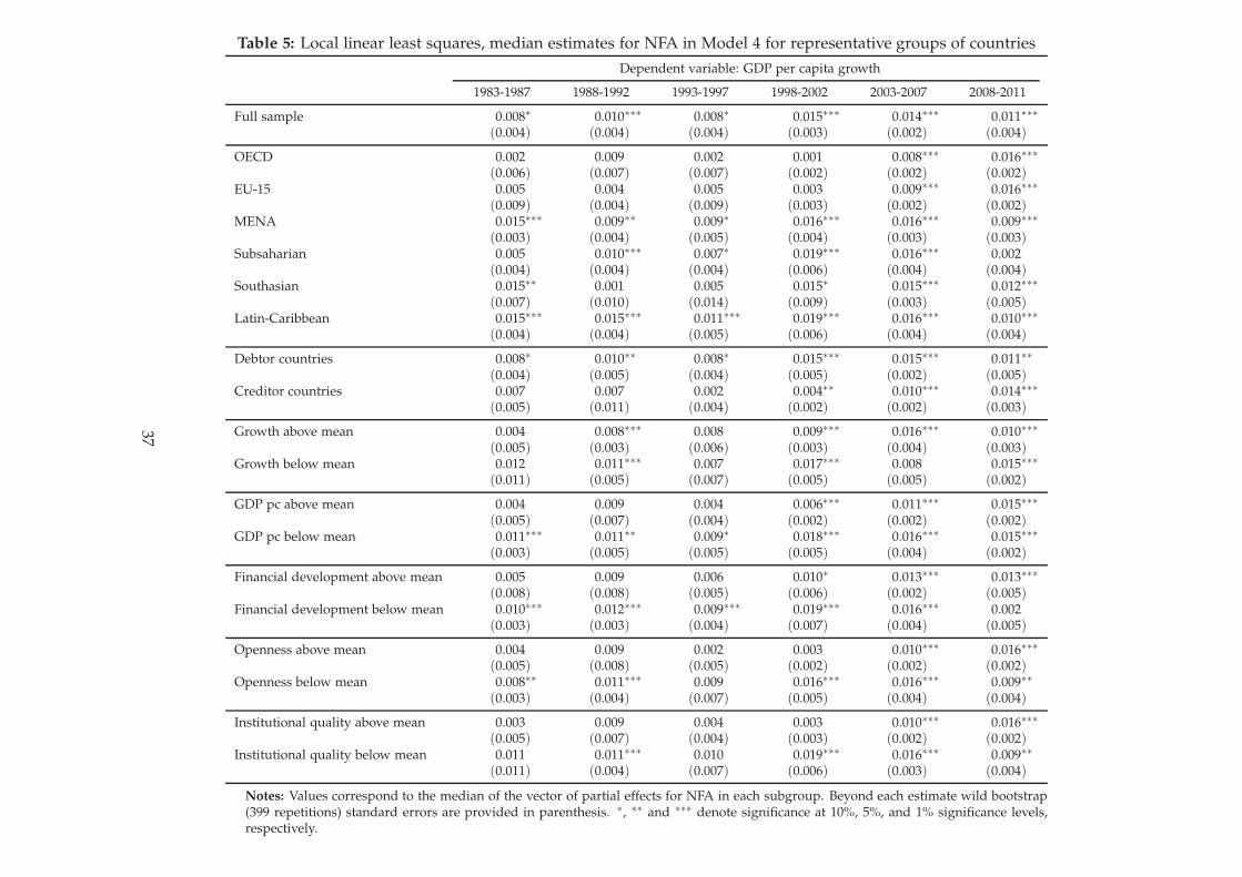
Table 5: Local linear least squares, median estimates for NFA in Model 4 for representative groups of countries
Dependent variable: GDP per capita growth
1983-1987 1988-1992 1993-1997 1998-2002 2003-2007 2008-2011
Full sample 0.008∗ 0.010∗∗∗ 0.008∗ 0.015∗∗∗ 0.014∗∗∗ 0.011∗∗∗
(0.004) (0.004) (0.004) (0.003) (0.002) (0.004)
OECD 0.002 0.009 0.002 0.001 0.008∗∗∗ 0.016∗∗∗
(0.006) (0.007) (0.007) (0.002) (0.002) (0.002)EU-15 0.005 0.004 0.005 0.003 0.009∗∗∗ 0.016∗∗∗
(0.009) (0.004) (0.009) (0.003) (0.002) (0.002)MENA 0.015∗∗∗ 0.009∗∗ 0.009∗ 0.016∗∗∗ 0.016∗∗∗ 0.009∗∗∗
(0.003) (0.004) (0.005) (0.004) (0.003) (0.003)Subsaharian 0.005 0.010∗∗∗ 0.007∗ 0.019∗∗∗ 0.016∗∗∗ 0.002
(0.004) (0.004) (0.004) (0.006) (0.004) (0.004)Southasian 0.015∗∗ 0.001 0.005 0.015∗ 0.015∗∗∗ 0.012∗∗∗
(0.007) (0.010) (0.014) (0.009) (0.003) (0.005)Latin-Caribbean 0.015∗∗∗ 0.015∗∗∗ 0.011∗∗∗ 0.019∗∗∗ 0.016∗∗∗ 0.010∗∗∗
(0.004) (0.004) (0.005) (0.006) (0.004) (0.004)
Debtor countries 0.008∗ 0.010∗∗ 0.008∗ 0.015∗∗∗ 0.015∗∗∗ 0.011∗∗
(0.004) (0.005) (0.004) (0.005) (0.002) (0.005)Creditor countries 0.007 0.007 0.002 0.004∗∗ 0.010∗∗∗ 0.014∗∗∗
(0.005) (0.011) (0.004) (0.002) (0.002) (0.003)
Growth above mean 0.004 0.008∗∗∗ 0.008 0.009∗∗∗ 0.016∗∗∗ 0.010∗∗∗
(0.005) (0.003) (0.006) (0.003) (0.004) (0.003)Growth below mean 0.012 0.011∗∗∗ 0.007 0.017∗∗∗ 0.008 0.015∗∗∗
(0.011) (0.005) (0.007) (0.005) (0.005) (0.002)
GDP pc above mean 0.004 0.009 0.004 0.006∗∗∗ 0.011∗∗∗ 0.015∗∗∗
(0.005) (0.007) (0.004) (0.002) (0.002) (0.002)GDP pc below mean 0.011∗∗∗ 0.011∗∗ 0.009∗ 0.018∗∗∗ 0.016∗∗∗ 0.015∗∗∗
(0.003) (0.005) (0.005) (0.005) (0.004) (0.002)
Financial development above mean 0.005 0.009 0.006 0.010∗ 0.013∗∗∗ 0.013∗∗∗
(0.008) (0.008) (0.005) (0.006) (0.002) (0.005)Financial development below mean 0.010∗∗∗ 0.012∗∗∗ 0.009∗∗∗ 0.019∗∗∗ 0.016∗∗∗ 0.002
(0.003) (0.003) (0.004) (0.007) (0.004) (0.005)
Openness above mean 0.004 0.009 0.002 0.003 0.010∗∗∗ 0.016∗∗∗
(0.005) (0.008) (0.005) (0.002) (0.002) (0.002)Openness below mean 0.008∗∗ 0.011∗∗∗ 0.009 0.016∗∗∗ 0.016∗∗∗ 0.009∗∗
(0.003) (0.004) (0.007) (0.005) (0.004) (0.004)
Institutional quality above mean 0.003 0.009 0.004 0.003 0.010∗∗∗ 0.016∗∗∗
(0.005) (0.007) (0.004) (0.003) (0.002) (0.002)Institutional quality below mean 0.011 0.011∗∗∗ 0.010 0.019∗∗∗ 0.016∗∗∗ 0.009∗∗
(0.011) (0.004) (0.007) (0.006) (0.003) (0.004)
Notes: Values correspond to the median of the vector of partial effects for NFA in each subgroup. Beyond each estimate wild bootstrap(399 repetitions) standard errors are provided in parenthesis. ∗, ∗∗ and ∗∗∗ denote significance at 10%, 5%, and 1% significance levels,respectively.
37

Table 6: Nonparametric comparison (Li, 1996) of theestimated densities for different groups inModel 4
Compared distributions t-statistic
OECD vs. EU-15 −1.227OECD vs. MENA 3.872∗∗∗
OECD vs. Subsaharian 6.987∗∗∗
OECD vs. South-Asian 1.797∗∗
OECD vs. Latin-Caribbean 23.540∗∗∗
EU-15 vs. MENA 3.039∗∗∗
EU-15 vs. Subsaharian 5.143∗∗∗
EU-15 vs. South-Asian 2.262∗∗
EU-15 vs. Latin-Caribbean 17.260∗∗∗
MENA vs. Subsaharian 1.080MENA vs. South-Asian −0.163MENA vs. Latin-Caribbean 1.980∗∗
Subsaharian vs. South-Asian 1.075Subsaharian vs. Latin-Caribbean 10.711∗∗∗
South-Asian vs. Latin-Caribbean 1.874∗∗
1983–1987 vs. 1988–1992 3.312∗∗∗
1983–1987 vs. 1993–1997 6.170∗∗∗
1983–1987 vs. 1998–2002 2.778∗∗∗
1983–1987 vs. 2003–2007 13.358∗∗∗
1983–1987 vs. 2008–2011 4.275∗∗∗
1988–1992 vs. 1993–1997 1.632∗
1988–1992 vs. 1998–2002 10.002∗∗∗
1988–1992 vs. 2003–2007 4.099∗∗
1988–1992 vs. 2008–2011 0.1181993–1997 vs. 1998–2002 20.456∗∗∗
1993–1997 vs. 2003–2007 17.361∗∗∗
1993–1997 vs. 2008–2011 8.613∗∗∗
1998–2002 vs. 2003–2007 12.832∗∗∗
1998–2002 vs. 2008–2011 6.307∗∗∗
2003–2007 vs. 2008–2011 2.363∗∗∗
Above vs. below mean growth rate 0.709Debtor countries vs. creditor countries 0.220Above vs. below mean GDP pc 5.322∗∗∗
Above vs. below mean financial development 1.716∗
Above vs. below mean openness 2.993∗∗∗
Above vs. below mean institutional quality 17.153∗∗∗
Notes: Under the null hypothesis (H0 : h(x) = g(x)), the twodistributions are equal. Under the alternative (H1 : h(x) 6=g(x)), they differ statistically. ∗, ∗∗ and ∗∗∗ denote significanceat 10%, 5%, and 1% significance levels, respectively.
38
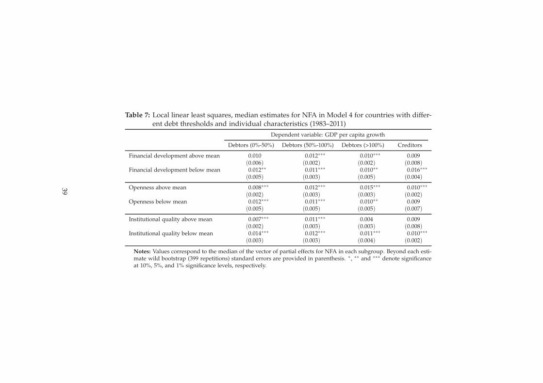
Table 7: Local linear least squares, median estimates for NFA in Model 4 for countries with differ-ent debt thresholds and individual characteristics (1983–2011)
Dependent variable: GDP per capita growth
Debtors (0%-50%) Debtors (50%-100%) Debtors (>100%) Creditors
Financial development above mean 0.010 0.012∗∗∗ 0.010∗∗∗ 0.009(0.006) (0.002) (0.002) (0.008)
Financial development below mean 0.012∗∗ 0.011∗∗∗ 0.010∗∗ 0.016∗∗∗
(0.005) (0.003) (0.005) (0.004)
Openness above mean 0.008∗∗∗ 0.012∗∗∗ 0.015∗∗∗ 0.010∗∗∗
(0.002) (0.003) (0.003) (0.002)Openness below mean 0.012∗∗∗ 0.011∗∗∗ 0.010∗∗ 0.009
(0.005) (0.005) (0.005) (0.007)
Institutional quality above mean 0.007∗∗∗ 0.011∗∗∗ 0.004 0.009(0.002) (0.003) (0.003) (0.008)
Institutional quality below mean 0.014∗∗∗ 0.012∗∗∗ 0.011∗∗∗ 0.010∗∗∗
(0.003) (0.003) (0.004) (0.002)
Notes: Values correspond to the median of the vector of partial effects for NFA in each subgroup. Beyond each esti-mate wild bootstrap (399 repetitions) standard errors are provided in parenthesis. ∗, ∗∗ and ∗∗∗ denote significanceat 10%, 5%, and 1% significance levels, respectively.
39

Table 8: Local linear least squares, individual estimates for NFA in Model 4 for representativecountries
Dependent variable: GDP per capita growth
1983-1987 1988-1992 1993-1997 1998-2002 2003-2007 2008-2011
EEUU 0.004 0.018∗∗∗ 0.003 −0.001 0.008∗∗∗ 0.018∗∗∗
(0.008) (0.006) (0.008) (0.003) (0.002) (0.002)Germany 0.009 0.000 −0.001 0.008∗∗∗ 0.018∗∗∗
(0.007) (0.005) (0.003) (0.002) (0.002)Argentina 0.014∗ 0.016∗∗∗ 0.010∗∗∗ 0.012∗∗∗ 0.016∗∗∗ 0.015∗∗∗
(0.008) (0.004) (0.004) (0.002) (0.003) (0.004)Spain 0.008∗∗∗ 0.001 0.003 0.005∗∗ 0.008∗∗∗ 0.013∗∗∗
(0.002) (0.010) (0.004) (0.003) (0.002) (0.002)Greece −0.004 0.002 0.004 0.006∗∗∗ 0.010∗∗∗ 0.019∗∗∗
(0.004) (0.006) (0.004) (0.002) (0.002) (0.003)China 0.020∗∗∗ 0.015∗∗∗ 0.013∗∗∗ 0.015∗∗∗ 0.010∗∗∗ 0.015∗∗∗
(0.004) (0.004) (0.004) (0.005) (0.002) (0.003)
Notes: Beyond each estimate wild bootstrap (399 repetitions) standard errors are provided in parenthesis. ∗, ∗∗ and∗∗∗ denote significance at 10%, 5%, and 1% significance levels, respectively.
40

Figure 1: Net foreign assets, international comparison in 2007
CREDITORSDEBTORS (0%−50%)DEBTORS (50%−100%)DEBTORS (>100%)NO DATA
41

Figure 2: Net foreign assets (1983–2011)
1985 1990 1995 2000 2005 2010
Year
NFA
−2.0
−1.5
−1.0
−0.5
0.0
0.5
1.0
1.5
2.0 OECDEU−15
MENASUBSAHARIAN
LATIN CARIBBEANSOUTH ASIAN
(a) NFA, groups of countries
1985 1990 1995 2000 2005 2010
Year
NFA
−1.5
−1.1
−0.7
−0.3
0.1
0.5
0.9 GERMANYEE.UU.
SPAINGREECE
ARGENTINACHINA
(b) NFA, particular countries
−3
−2
−1
01
23
1983−1987 1988−1992 1993−1997 1998−2002 2003−2007 2008−2011
(c) NFA by period, violin plots
Notes: In the violin plots, the white bullet inside the box represents the median value and the black box contains 50% of the sample (first and third quartilescorrespond to the bottom and the top of the box, respectively). The vertical bars represent observations beyond these limits and, finally, the kernel densityoverlaying the boxplot displays the probability mass at the different values of the represented variable.
42

Figure 3: Net foreign assets, estimated coefficients
−0.04 −0.02 0.00 0.02 0.04 0.06
02
04
06
08
0
NFA, estimated coefficient
De
nsity
Model 1Model 2Model 3Model 4
(a) NFA, Kernel density for different models
−0.04 −0.02 0.00 0.02 0.04 0.06
−0.
04−
0.02
0.00
0.02
0.04
0.06
NFA, Estimated coefficient
NFA
, Est
imat
ed c
oeffi
cien
t
(b) NFA, 45o plot for estimates in Model 4
43

Figure 4: Net foreign assets, estimates for particular groups in Model 4
−0.04 −0.02 0.00 0.02 0.04
02
04
06
08
0
NFA, estimated coefficient
De
nsity o
f co
un
trie
s
OECDEU−15MENASUBSAHARIANSOUTH ASIANLATIN CARIBBEAN
−0.04 −0.02 0.00 0.02 0.04 0.06
01
02
03
04
05
0
NFA, estimated coefficient
De
nsity o
f co
un
trie
s
DEBTOR COUNTRIESCREDITOR COUNTRIES
−0.04 −0.02 0.00 0.02 0.04
01
02
03
04
05
0
NFA, estimated coefficient
De
nsi
ty o
f co
un
trie
s
GROWTH ABOVE MEANGROWTH BELOW MEAN
−0.04 −0.02 0.00 0.02 0.04
01
02
03
04
05
0
NFA, estimated coefficient
De
nsi
ty o
f co
un
trie
s
GDP pc ABOVE MEANGDP pc BELOW MEAN
−0.04 −0.02 0.00 0.02 0.04
01
02
03
04
05
06
0
NFA, estimated coefficient
De
nsi
ty o
f co
un
trie
s
FINANCIAL DEVELOPMENT ABOVE MEANFINANCIAL DEVELOPMENT BELOW MEAN
−0.04 −0.02 0.00 0.02 0.04
010
2030
4050
NFA, estimated coefficient
Den
sity
of c
ount
ries
OPENNESS ABOVE MEANOPENNESS BELOW MEAN
−0.04 −0.02 0.00 0.02 0.04
010
2030
4050
60
NFA, estimated coefficient
Den
sity
of c
ount
ries
INSTITUTIONAL QUALITY ABOVE MEANINSTITUTIONAL QUALITY BELOW MEAN
−0.04 −0.02 0.00 0.02 0.04 0.06
02
04
06
08
0
NFA, estimated coefficient
De
nsity
1983−19871988−19921993−19971998−20022003−20072008−2011
44