exploring new neural architectures for adaptation to
TRANSCRIPT

The University of Tokyo
DoctorThesis
博⼠論⽂
Exploring New Neural Architectures forAdaptation to Complex Worlds
(新しい構造に基づいて複雑性に対処するニューラルネットワークの研究)
Author:Sinapayen Lanaシナパヤ ラナ

THE UNIVERSITY OF TOKYO
PrologueDepartment of Multidisciplinary SciencesGraduate School of Arts and Sciences
Doctor
Exploring New Neural Architectures for Adaptation to Complex Worlds
by Sinapayen Lana
Action, Prediction, Classification.
The world is a dynamical system producing countless complex data streams: noisy,stochastic, aperiodic data. To manipulate the environment to its advantage, an organ-ism needs to filter these data streams and produce appropriate actions. The efficiencyof actions is improved by predicting consequences, and the efficiency of predictions isimproved by classifying inputs. Yet the amount of energy available to living organismsis limited, and these three functions cannot afford being both slow and computationallyexpensive. In this thesis, we present two algorithms to help machines learn from complexinput and produce appropriate outputs while optimizing the computational cost.

Contents
Prologue i
Contents ii
List of Figures iv
Abbreviations xi
1 Introduction 1
2 Learning by Stimulation Avoidance 62.1 Background . . . . . . . . . . . . . . . . . . . . . . . . . . . . . . . . . . . 62.2 Model . . . . . . . . . . . . . . . . . . . . . . . . . . . . . . . . . . . . . . 92.3 LSA is Sufficient to Explain Biological Results . . . . . . . . . . . . . . . 12
2.3.1 Superficial selective learning experiment . . . . . . . . . . . . . . . 132.3.2 Dynamics of LSA in 2-Neuron Paths . . . . . . . . . . . . . . . . . 19
2.3.2.1 Dynamics in a single synapse . . . . . . . . . . . . . . . . 192.3.2.2 Effect-based differentiation of stimuli . . . . . . . . . . . 22
2.3.3 Dynamics of LSA in 3-Neuron Paths . . . . . . . . . . . . . . . . . 232.4 Burst Suppression by Adding Noise . . . . . . . . . . . . . . . . . . . . . . 25
2.4.1 Selective Learning with burst suppression . . . . . . . . . . . . . . 252.4.2 Parameter Exploration . . . . . . . . . . . . . . . . . . . . . . . . . 28
2.5 Burst Suppression by Short Term Plasticity . . . . . . . . . . . . . . . . . 292.6 Embodied Application: Wall Avoidance with a Robot . . . . . . . . . . . 302.7 Discussion . . . . . . . . . . . . . . . . . . . . . . . . . . . . . . . . . . . . 34
3 The Epsilon Network 393.1 Background . . . . . . . . . . . . . . . . . . . . . . . . . . . . . . . . . . . 393.2 Model . . . . . . . . . . . . . . . . . . . . . . . . . . . . . . . . . . . . . . 42
3.2.1 Network architecture . . . . . . . . . . . . . . . . . . . . . . . . . . 433.2.2 Creating and updating prediction weights . . . . . . . . . . . . . . 45
3.2.2.1 Creating PrW . . . . . . . . . . . . . . . . . . . . . . . . 453.2.3 Creating and updating pattern weights . . . . . . . . . . . . . . . . 48
3.2.3.1 Creating a PaW . . . . . . . . . . . . . . . . . . . . . . . 483.2.3.2 Updating a PaW . . . . . . . . . . . . . . . . . . . . . . . 493.2.3.3 Decreasing the number of neurons and weights . . . . . . 52
ii

Contents iii
3.2.4 Short Term Memory and Attention Mechanism . . . . . . . . . . . 533.2.5 Hierarchical structures . . . . . . . . . . . . . . . . . . . . . . . . . 533.2.6 Modularity . . . . . . . . . . . . . . . . . . . . . . . . . . . . . . . 54
3.2.6.1 User Interface . . . . . . . . . . . . . . . . . . . . . . . . 583.3 Results . . . . . . . . . . . . . . . . . . . . . . . . . . . . . . . . . . . . . . 59
3.3.1 Minimal automaton . . . . . . . . . . . . . . . . . . . . . . . . . . 593.3.2 Clean or noisy environments . . . . . . . . . . . . . . . . . . . . . 613.3.3 Complex data stream and simple data stream . . . . . . . . . . . . 633.3.4 Surprising events . . . . . . . . . . . . . . . . . . . . . . . . . . . . 693.3.5 Full model and long videos . . . . . . . . . . . . . . . . . . . . . . 693.3.6 Comparison with the state of the art: PredNet . . . . . . . . . . . 73
3.4 Discussion . . . . . . . . . . . . . . . . . . . . . . . . . . . . . . . . . . . . 74
4 General Discussion 77
Bibliography 82
Acknowledgements 82

List of Figures
1.1 Evolutionary needs and their corresponding solutions. An or-ganism needs behavior; this need is met by the evolution of actuators tomodify the world. It also needs to be empowered, which depends on pre-diction to anticipate appropriate actions. Finally, it needs to generalizethese predictions, which is the role of classification. Prediction emergesfrom the need for better actions, and classification emerges from the needfor better predictions. . . . . . . . . . . . . . . . . . . . . . . . . . . . . . 3
2.1 The Stimulus Regulation Principle (SRP). (a) The SRP postulatesthat the structure of the network randomly changes when focal electricstimulation is applied, creating new paths (modifiability). (b) When thestimulation is stopped, the structure of the network stops changing (sta-bility). This idea does not explain how newly formed paths would avoidbeing destroyed when stimulation is applied to the network again like inShahaf’s training method. . . . . . . . . . . . . . . . . . . . . . . . . . . . 7
2.2 Strengthening or pruning of synapses according to LSA. Thetiming of the stimulation to a pre-synaptic neuron relative to the firingof the post-synaptic neuron the causes the strengthening or pruning ofthe synapse. If the stimulation stops just after the post-synaptic spike,the synapse is strengthened; if the stimulation starts just after the post-synaptic spike, the synapse is pruned. . . . . . . . . . . . . . . . . . . . . 8
2.3 Equations and dynamics of regular spiking and fast spiking neu-rons simulated with the Izhikevich model. Equations and dynamicsof regular spiking and fast spiking neurons simulated with the Izhikevichmodel. . . . . . . . . . . . . . . . . . . . . . . . . . . . . . . . . . . . . . . 10
2.4 The Spike-Timing Dependent Plasticity (STDP) function gov-erning the weight variation ∆w of the synapse from neuron a to neuronb depending on the relative spike timing s = tb − ta. A = 0.1; τ = 20 ms. . 11
2.5 The Shahaf experiment reformulated as a game. The networkcontrols a spaceship. There is one possible action: shooting, and onebinary input: presence or absence of an alien. Shooting destroys thealien. When an alien appears, the network’s ”eye neurons” are stimulated(Input Zone). If Output Zone A fires, the spaceship shoots. If OutputZone B fires at the same time as Output Zone B, the command is cancelledand the spaceship does not shoot. . . . . . . . . . . . . . . . . . . . . . . . 14
2.6 Evolution of the reaction times of 2 successful neural networksat the selective learning task. 20 networks were simulated, 18 ofwhich successfully learned the task (Table 2.1). Red lines represent whenthere was no response from the network. A learning curve is clearly visible. 15
iv

List of Figures v
2.7 A typical learning curve. During the initialization phase, the networkactivity is high, causing randomly short reaction times. In the explo-ration phase, the activity has stabilized and the reaction times are long;sometimes the expected output never fires. During the learning phase,the reaction time steadily decreases. Finally the behavior is learned andthe reaction time stabilizes at short values. . . . . . . . . . . . . . . . . . 15
2.8 Raster plot of the temporal firing of the network at differentphases of the experiment. During initialization, the network’s activ-ity is strong and highly synchronized (global bursts). During learning,the bursts are more common but shorter and less synchronized. Afterlearning, the network has very high activity with numerous bursts. . . . . 16
2.9 Weight matrix after learning. Initially the matrix is random, butafter learning a structure is somewhat visible. Weights from the inputneurons to all other neurons are high, including weights to Output Zone B. 17
2.10 Simple Learning experiment with no inhibitory neurons in thenetwork. The initialization phase is as long as in the original conditions,but the network is stuck in the exploration phase and never reaches thelearning phase. . . . . . . . . . . . . . . . . . . . . . . . . . . . . . . . . . 18
2.11 Simple Learning experiment with no external stimulation. Theinitialization phase is as long as in the original conditions, but with no wayto differentiate the correct firing pattern from other firing patterns, thenetwork has no proper exploration phase and does not reach the learningphase. The desired firing pattern stops being exhibited. . . . . . . . . . . 18
2.12 Experimental setup. The minimal network counts 2 neurons and 1synapse. Random noise m is added as input to both neurons. An exter-nal stimulation e0 is applied to N0. The dynamics of e0 depend on theexperimental conditions. . . . . . . . . . . . . . . . . . . . . . . . . . . . . 20
2.13 The three conditions used in Experiment 1 summarized as araster plot. The rectangles represent neuronal spikes. The externalstimulation e0 causes N0 to fire rhythmically; firing of N0 causes stimu-lation in N1. In real conditions, the noise and synaptic weight variationscause less regular spiking. . . . . . . . . . . . . . . . . . . . . . . . . . . . 20
2.14 Weight variation in one synapse depending on the effect of post-synaptic neuron firing. The principle of LSA is verified: behaviorsconducting to stimulation avoidance are reinforced via synaptic strength-ening or synaptic pruning. The default dynamics of STDP lead to weightstrengthening in neutral conditions, behavior which can be partly avoidedby applying a decay function. . . . . . . . . . . . . . . . . . . . . . . . . . 21
2.15 Augmented experimental setup: 3 neurons and 2 synapses. Randomnoise m is added as input to all neurons. The dynamics of the exter-nal stimulations e0 and e2 are different and depend on the experimentalconditions. . . . . . . . . . . . . . . . . . . . . . . . . . . . . . . . . . . . . 22
2.16 Parallel processing of two input synapses in one neuron. Onesynapse is pruned while the other is strengthened: the post-synaptic neu-ron can process inputs from both pre-synaptic neurons simultaneously.. . . . . . . . . . . . . . . . . . . . . . . . . . . . . . . . . . . . . . . . . . 23

List of Figures vi
2.17 Dynamics of weight changes induced by LSA in small networksof 3 neurons. A) Reinforcement: spiking of neuron 2 stops the stimula-tion in neuron 0. The direct weight w0,2 grows faster than other weights,even when starting at a lower value. B) Artificially fixing the direct weightw0,2 to 0, a longer pathway of 2 connections 0 → 1 → 2 is established.C) Pruning: spiking of neuron 2 starts external stimulation to neuron 0.As a result, w0,2 is pruned. . . . . . . . . . . . . . . . . . . . . . . . . . . 24
2.18 Raster plots of a regular network (activity concentrated in bursts)and a network of which parameters have been tuned to reducebursting and enhance desynchronized spiking. The desynchroniz-ing effect of sparsely connecting the network and increasing the noise areclearly visible. . . . . . . . . . . . . . . . . . . . . . . . . . . . . . . . . . . 26
2.19 Trajectory of the network in the two-dimensional space of thefiring rates of Output Zone A and Output Zone B. Using LSA,we can steer the network in this space; by contrast, the “reinforcementonly” experiment maintains the network balanced relatively to the twofiring rates. (a) leads to the low external stimulation region but (b) doesnot. Statistical results for N = 20 networks. . . . . . . . . . . . . . . . . . 27
2.20 Performance of learning depending of network connectivity andinitial weights variance. Learnability is defined as the average dif-ference between the firing rate of the Output Zone during the first 100seconds and the last 100 seconds. The ideal region of the parameter spaceto obtain good learning results is between 20 and 30 connections per neu-ron. By comparison, the variance has less influence. Statistical results forN= 20 networks for each parameter set. . . . . . . . . . . . . . . . . . . . 28
2.21 Firing rate distribution. This figure shows the cumulative number ofneurons in each firing rate bin for 20 networks. Before learning (first 100 s,blue), most neurons have a very low firing rate (leftmost peak) except forthe input neurons (rightmost peak). After learning (last 100 s, red), theneurons are distributed in 2 groups: low firing rate (2nd peak from theleft) and medium firing rate. 50 % of the Output Zone B neurons arecontained in the zone marked I; 50 % of the Output Zone A neurons arecontained in the zone marked II. . . . . . . . . . . . . . . . . . . . . . . . 30
2.22 Robot simulation. The robot has distance sensors and must learn tostay away from the arena’s walls. . . . . . . . . . . . . . . . . . . . . . . . 31
2.23 Learning curves of the wall avoidance task. The robot is consideredto be “close” to a wall if it is less than 80 pixels from the wall, whichcorresponds to the range of its distance sensors. The results show thatrandom steering due to high random activity in the network leads tospending 64% of the time close to walls, while learning due to LSA leads toonly 43% time spent close to walls. Statistical results for N= 20 networks,standard error is indicated. . . . . . . . . . . . . . . . . . . . . . . . . . . 32
2.24 The track of a “good performing” robot with the standard model.The crossing lines are the limits beyond which the robot is considered tobe close to a wall. Because the robot spends most of its time spinning onitself as an effect of the noise, it barely gets a chance to get close to thewall. Its “only 7% of the time close to a wall” performance is not reallya measure of its actual usefulness. . . . . . . . . . . . . . . . . . . . . . . . 34

List of Figures vii
2.25 Learnability of wall avoidance based on sensor sensitivity. Highnumbers on the x axis indicate high sensitivity. Under 5 mV, the taskcannot be learned; learnability improves until 7 mV, leading to the maxi-mum performance of the robot. The open loop and closed loop results forthe same sensitivity of 8 mV are reported from Fig 2.23. We have omit-ted the open loop cases as they are insensitive to the walls, but shown forthe case at the sensor sensitivity = 8 mV. Statistical results for N= 20networks with standard error. . . . . . . . . . . . . . . . . . . . . . . . . . 35
3.1 Conceptual view of online optimization in the ϵ-network. Thenetwork produces predictions from the input. Errors in this predictioncause surprise, which is used to add neurons and weights at appropri-ate locations in the network, improving future predictions. Periodically,neurons producing similar predictions are fused together, reducing thenumber of neurons and weights in the network. . . . . . . . . . . . . . . . 40
3.2 Classification and Prediction as interdependent functions. Ini-tially, there are no weights in the network and each neurons is simplyactivated from stimulation in its receptive field. During learning, newneurons and weights can be added; neurons can also be fused together(”snapped”). Snapped neurons represent classes. Pattern weights linkseveral subclasses to the superclass they belong to. Prediction weightsrepresent probabilistic time transitions between two neurons. Predictionweights determine which neurons can be snapped, and pattern weightscarry predictions down to their subclasses, closing the classification-predictionloop. . . . . . . . . . . . . . . . . . . . . . . . . . . . . . . . . . . . . . . . 43
3.3 Neurons sensitive to different shades of gray. Because we use visualimages as input, we can think of these neurons as being on different layers;in reality, there is no concept of layer in the network and all neurons in amodule can communicate together. . . . . . . . . . . . . . . . . . . . . . . 45
3.4 Network before adding weights and neurons. The greyscale inputis discretized so that the area has 6 sensors respectively activated by oneof 6 shades of grey. Here we show the receptive field of neurons sensitiveto black. . . . . . . . . . . . . . . . . . . . . . . . . . . . . . . . . . . . . . 47
3.5 Rule of creation of a prediction weight. The weight is created if aneuron is surprised (the neuron is activated unexpectedly). The predic-tion value p is used to predict whether the output neuron will be activatedat the next timestep, and updated during learning. . . . . . . . . . . . . . 48
3.6 Rule of update of a prediction weight. The prediction value p is updatedby counting how many times B is activated after A, yielding the exactprobability of activation. . . . . . . . . . . . . . . . . . . . . . . . . . . . . 49
3.7 Creation of a pattern weight. When prediction weights from A0..2 toB already exist but none can accurately predict B because the probabilityon each weight is too small, B will continue being surprised. When thishappens we create a pattern weight with A0..2 as input and a new neuronC as output. We also add a prediction weight (p = 1) from C to B. Nexttime that all 3 of A0..2 are activated, C will also be activated, and B willbe correctly predicted. . . . . . . . . . . . . . . . . . . . . . . . . . . . . . 50

List of Figures viii
3.8 Update rule of the pattern weight. In a), the PaW is made only ofstrands with p=1. According to the activation rule 100% of the strandswith p = 1 should be activated for the PaW to be activated, so withonly A0 and A1 activated for the PaW is not activated. Therefore thecondition of activation of the PaW must be relaxed by decreasing thevalue of A2. b) The PaW was not activated, so C was not activatedand B could not be predicted, leading to surprise. The surprise meansthat the PaW must be updated. c) The weight of each strand is updateddepending on whether the input neuron was activated at t − 1. A0 andA1 were activated at t − 1 so their weights are still p = 1; A2 was notactivated so its weight is decreased to p = 0.5. d) Next time that A0 andA1 are activated, this is sufficient to activate C and predict B. (50% ofneurons with p = 0.5 are also required to be activated; there is only onesuch neuron so it can be ignored.) . . . . . . . . . . . . . . . . . . . . . . 51
3.9 Example of snapping procedure: two neurons are fused together if theyhave the same output values; their input weights are reported to the fusedneuron. . . . . . . . . . . . . . . . . . . . . . . . . . . . . . . . . . . . . . 53
3.10 Hierarchical prediction. Pattern weights introduce the possibility forhierarchical prediction from neuron (class) A to neuron (class) B and allof the neurons that are part of a pattern that can activate B, instead ofhaving prediction weights from A to each of B’s sub-classes. . . . . . . . . 54
3.11 Generalizing using hierarchical predictions while avoiding over-prediction with inhibitory weights. The network is trained on simpletime series and learns the patterns for bombs and fires. Snapping causesthe neurons for ”fire” to be fused, generalizing the concept of fire by losingspatial information. When ”fire” is predicted, the network does not knowat which position. Inhibitory weights allow the prediction to use localspatial information from the lower levels of the network. . . . . . . . . . . 55
3.12 Creation of an inhibitory weight. Inhibitory weights are createdfrom neurons that were correctly predicted to false positive neurons thatwere predicted but not activated. The update rule of the weight value issimilar to the rule for prediction weights: p is the number of times thatthe post-synaptic neuron’s prediction was correctly inhibited (inhibitedand not activated at t+1) divided by the total number of activations ofthe pre-synaptic neuron. . . . . . . . . . . . . . . . . . . . . . . . . . . . . 56
3.13 Division of the network into modules. Each module takes inputfrom a small part of the image. Periodically during learning, higher levelneurons from existing modules are added as input to the neurons of thehierarchically higher modules, creating a possibility for inter-module com-munication. One neuron or one pixel cannot belong to several modulesat once, so this is not similar to a convolutional network. . . . . . . . . . . 57
3.14 User Interface of the program. On the left from top to bottom itdisplays the source image, its coarse grained version, as well as the networkprediction for the next image. On the right we can see the completenetwork or parts of it, in this case the neurons for the first gray scalevalue. On top we can control the speed, change the network display, saveand load existing networks. . . . . . . . . . . . . . . . . . . . . . . . . . . 58

List of Figures ix
3.15 User Interface of the program. This experiment used a modularstructure: image division is shown by red lines. The network structure isnot displayed. In this experiment we used higher resolution images andby step 30 the prediction is excellent. White spots indicate the placeswhere the network does not have a predicted value. . . . . . . . . . . . . . 59
3.16 Simple sequence of 3 images of a ball falling. . . . . . . . . . . . . . 593.17 Evolution of the number of neurons (left) and of probability
weights (right). After a few snapping procedures, the number of neu-rons falls to 4 (one neuron for each position of the ball and a 4th neu-ron gathering all unused inputs like the grayscale values absent from thedataset); after the initial increase, the final number of PrW is 3. . . . . . 60
3.18 Evolution of the network’s topology: t = 50 and t = 200. The finaltopology perfectly represents the automaton of the time series, with eachneurons corresponding to a state and each weight to a transition withprobability 1. The 4th neuron, with no output weights, is omitted. . . . . 61
3.19 Detail of the final receptive field of each neuron. As the result ofthe snapping procedure, each neuron can now be activated by any of thesensors in large receptive fields, as activation of any of these sensors issufficient to predict the next frame accurately. The receptive fields spanthe width and height of the image but also several greyscale values. Fromthe neurons activation, we can still deduce which image the network isseeing. . . . . . . . . . . . . . . . . . . . . . . . . . . . . . . . . . . . . . . 62
3.20 Emergence of classes in the simple experiment. The neurons ineach group in (a) have similar output weights, therefore are snapped to-gether, resulting in (b). The unused neurons (from the background andfrom greyscales never stimulated in this experiment) also have the sameoutput weights and are snapped together into one neuron with no weights. 63
3.21 Sequence with a cue: we introduce a variation in the ball position onthe 3rd and 6th frames. . . . . . . . . . . . . . . . . . . . . . . . . . . . . 63
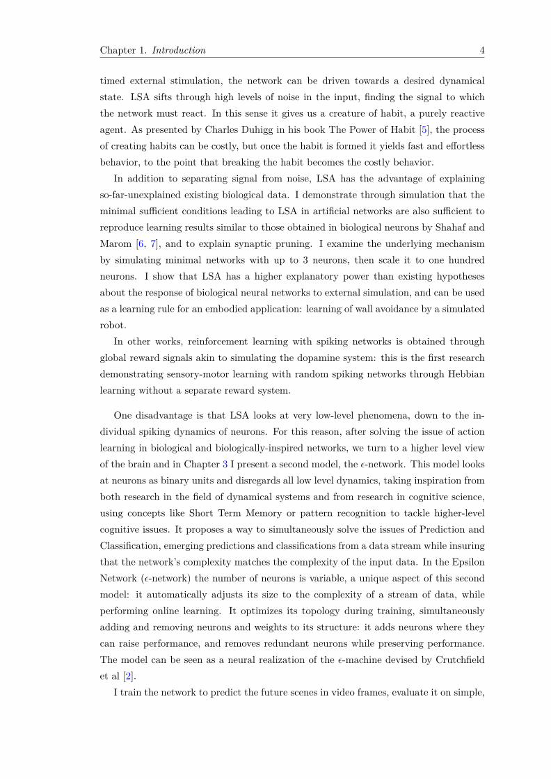
3.22 Evolution of the number of neurons (left) and of probabilityweights (right) for the modified sequence. The final number ofneurons is 6; the number of probability weights rises more sharply thanfor the simple sequence, but then decreases from more than 9,000 to only11 PrW. . . . . . . . . . . . . . . . . . . . . . . . . . . . . . . . . . . . . . 64
3.23 Examples of frames from the KITTI dataset . . . . . . . . . . . . . . . . . 643.24 Evolution of the number of neurons (left) and of prediction
weights (right) on a clean video (blue lines) and a noisy version of thesame video (red lines). The final results capture nicely the complexityinduced by trying to predict a noisy dataset. . . . . . . . . . . . . . . . . 65
3.25 Evolution of the total number of prediction weights (left) andof the number of effective prediction weights (p > 0.9, right) on aclean video (blue lines) and a noisy version of the same video (red lines).There are more weights in the network for the noisy video, but theseadditional weights have low predictive power and the number of strongprediction weights is the same for the noisy and non noisy video. . . . . . 65
3.26 Evolution of the surprise in the network with and without noise.The value slowly decreases as the networks evolves. At t = 82 (blackline), the video sequence starts a new loop which is a sudden and highlysurprising event for the network. . . . . . . . . . . . . . . . . . . . . . . . 66

List of Figures x
3.27 Frames from a simple sequence (2 characters play the accordionin almost periodic motion, static background) and a complexsequence (a character rides a bicycle, the background changes) . 66
3.28 Evolution of the number of neurons (left) and of weights (right)for the two experiments. Although both videos have the same numberof frames, the number of neurons and connections is much higher for thecomplex video sequence. . . . . . . . . . . . . . . . . . . . . . . . . . . . . 67
3.29 Evolution of the number of effective weights (p > 0.9) for thesimple and complex videos. Unlike the results with or without noise,even when discounting the weak weights the complex video requires moreweights than the simple one. This is true complexity in the sense ofCrutchfield. . . . . . . . . . . . . . . . . . . . . . . . . . . . . . . . . . . . 67
3.30 Evolution of the surprise in the simple and complex task. Thesurprise decreases sharply at the beginning of either task, then stays stableat the network optimizes its size. . . . . . . . . . . . . . . . . . . . . . . . 68
3.31 Evolution of the surprise in the simple and complex task. Zoomon the first 150 steps shows small differences between the two time series,especially at the first loop of the videos, the surprise is higher for thecomplex video. . . . . . . . . . . . . . . . . . . . . . . . . . . . . . . . . . 68
3.32 Peak of new neurons indicating surprising events in the first150 frames. The first few timesteps the network has no knowledge, soeverything is surprising. After this naive period, all peaks correspond tosignificant events. . . . . . . . . . . . . . . . . . . . . . . . . . . . . . . . . 69
3.33 Peak of new neurons indicating surprising events in the first 300frames. The biggest peaks can be seen for scene changes, which are verymuch unpredictable. . . . . . . . . . . . . . . . . . . . . . . . . . . . . . . 70
3.34 Mean Squared Error of the predictions for snapping every 50steps, 100 steps, or not snapping at all. We can see that the errorgets smaller if we snap the network less often. This means that whenfusing neurons together, a small amount of information is lost that cannotbe recovered. . . . . . . . . . . . . . . . . . . . . . . . . . . . . . . . . . . 71
3.35 Mean Number of neurons for snapping every 50 steps, 100 steps,or not snapping at all. Snapping initially works as a method to reducethe number of neurons, but some information is lost by fusing neuronstoo early. Overtime this results in some bad predictions and number ofneurons greater than without snapping. . . . . . . . . . . . . . . . . . . . 72

Abbreviations
LSA Learning by Stimulation Avoidance
MSE Mean Squared Error
SRP Stimulus Regulation Principle
STDP Spike-Timing Dependent Plasticity
STP Short Term Plasticity
STM Short Term Memory
PrW Prediction Weight
PaW Pattern Weight
xi

Chapter 1
Introduction
The real world, compared to simulated models, contains massive amounts of informa-tion. The amount of information itself is not complexity, but the way this informationcomes together is referred as environmental complexity.
There are many definitions of complexity; two of these definitions seem particularlyrelevant to this work. In 1947, Weaver gave a definition that identified two subtypesof complexity [1] : disorganized complexity and organized complexity. Disorganizedcomplexity refers to data that is produced by many components of system loosely inter-acting together. This type of data looks complex if each point is observed in isolation,but can be described in a simple way using probability distributions: Brownian motionis an example of disorganized complexity. Organized complexity involves componentsstrongly coupled together, producing organized data that cannot be described using onlystatistics: Darwinian evolution is an example of organized complexity. In 1989, Crutch-fied [2] gave a different definition of complexity as being a mix between two types ofsimple systems: random systems, which look complex but are statistically simple, andperiodic systems, which are simple to predict. Systems in-between these two extremesqualify as complex. Weaver’s disorganized complexity seems to align with Crutchfield’srandom systems, while Weaver’s organized complexity is the same as Crutchfield’s truecomplexity.
So what is complex behavior for an agent? Behavior consists in selecting the rightactions from processing input data. Even in complex environments, agents do not haveaccess to all of the world’s information; they only have access to a small part of it, asdata streaming through their sensors. The combined sensory information forms theirUmwelt [3], and is entirely dependent on darwinian evolution. The kind of actionsthat an agent can perform is also totally dependent on evolution, and the amount of
1

Chapter 1. Introduction 2
information going from the controller to the actuators of an agent depends on the agent’sbody plan.
But even a minimally simplistic agent with one binary sensor (e.g. a touch sensor)and one binary actuator (e.g. a button-pushing appendage) could, in theory, exhibitcomplex behavior if its action decision process itself is complex, neither random norperiodic: for example, pushing the button only after receiving an extremely long binarystring as input, partially depending on hidden random internal states.
Behavior is the most basic need of an agent, and action is the evolutionary functionthat emerged to fulfill this need. By acting, the agent goes from being a simple self-reproducing machine to being an agent. The need for behavior created a need for twoother functions: prediction and classification. By predicting, the agent goes from simplyreacting to stimuli, to being proactive in anticipation for future stimuli. By classifying, itgoes from only predicting consequences of previously encountered stimuli, to predictingconsequences of all new stimuli belonging to known classes. Here classes are taken to beunits for prediction, as in Crutchfield’s Epsilon Machine: if two seemingly separate unitshave the same consequences (eg a sweet taste), they represent the same cause (sugaron your tongue) and belong to the same class (fruits). The more units in the EpsilonMachine, the more complex the original input stream.
Action, Prediction, Classification: by order of importance, these are the functions anorganism needs to use a complex environment to its advantage. Accordingly, not all 3are needed by all organisms and the functions emerge from the bottom up: predictionemerges from action and classification emerges from prediction. Fig. 1.1 shows howthese 3 functions are linked, and the environmental needs that have resulted into thesefunctions evolving. We can sketch out the following rules regarding the complexity ofthe agent’s cognitive processes:
• The complexity of a perfect action selection process has the number of possibleactions as a lower bound
• The complexity of a perfect predictive process has the number of known classes asa lower bound
• The complexity of a perfect classification process has the number of classes (causesexplaining a data stream) existing in the real world as a lower bound.
The hierarchy of evolution goes from the most basic need to the more complex: action,prediction, classification. In theory, there is no higher bound to the complexity of thecognitive process, as an infinitely complex prediction machine can always be constructed

Chapter 1. Introduction 3
ActionBehavior
Changing things to your advantage,obtaining information
EmpowermentKnowing consequences of your
actions, good or bad
GeneralisationMaking your predictions work in
different contexts
Prediction
Classification
Need Function
Emerges from
Emerges from
Improved by
Improved by
Direction of evolution
Figure 1.1: Evolutionary needs and their corresponding solutions. An organ-ism needs behavior; this need is met by the evolution of actuators to modify the world.It also needs to be empowered, which depends on prediction to anticipate appropriateactions. Finally, it needs to generalize these predictions, which is the role of classifi-cation. Prediction emerges from the need for better actions, and classification emerges
from the need for better predictions.
even to explain the simplest data stream. In reality, cognitive processes have a cost ofenergy, and evolution will always match the cost of cognition to the benefits of theactions: for two levels of cognitive complexity that produce the same results in termsof actions, evolution will favor the least complex one. The cognitive process must notbe too costly, and it does not even have to be perfect: it just has to be sufficient forthe agent’s needs, as brilliantly demonstrated by Hoffman [4]. Cognitive complexity istherefore bounded by the level of complexity of what the agent can perceive of the realworld through its sensory inputs (and optionally by the attentional mechanisms thatsort through this input).
How can we obtain similar results artificially, and program a machine to adjust itscognitive complexity to the environment so that prediction emerges from action andclassification emerges from prediction? In this thesis, I present two models of networks.
The first network, presented in Chapter 2, is inspired from biology and proposes alearning rule for networks of spiking neurons as a way for the brain to close the input-output loop via action. Action must have been the first function to evolve in simpleorganisms, and in this sense the model proposed here solves the oldest issue that mighthave been faced by nervous systems: how to associate desirable/undesirable inputs withthe actions that cause these inputs? No learning rule has so far been accepted as a generalsolution for networks of real neurons and biologically-inspired networks. We argue forthe existence of a principle allowing to steer the dynamics of biological and biologically-inspired neural networks: “Learning by Stimulation Avoidance” (LSA). Using carefully
Chapter 1. Introduction 4
timed external stimulation, the network can be driven towards a desired dynamicalstate. LSA sifts through high levels of noise in the input, finding the signal to whichthe network must react. In this sense it gives us a creature of habit, a purely reactiveagent. As presented by Charles Duhigg in his book The Power of Habit [5], the processof creating habits can be costly, but once the habit is formed it yields fast and effortlessbehavior, to the point that breaking the habit becomes the costly behavior.
In addition to separating signal from noise, LSA has the advantage of explainingso-far-unexplained existing biological data. I demonstrate through simulation that theminimal sufficient conditions leading to LSA in artificial networks are also sufficient toreproduce learning results similar to those obtained in biological neurons by Shahaf andMarom [6, 7], and to explain synaptic pruning. I examine the underlying mechanismby simulating minimal networks with up to 3 neurons, then scale it to one hundredneurons. I show that LSA has a higher explanatory power than existing hypothesesabout the response of biological neural networks to external simulation, and can be usedas a learning rule for an embodied application: learning of wall avoidance by a simulatedrobot.
In other works, reinforcement learning with spiking networks is obtained throughglobal reward signals akin to simulating the dopamine system: this is the first researchdemonstrating sensory-motor learning with random spiking networks through Hebbianlearning without a separate reward system.
One disadvantage is that LSA looks at very low-level phenomena, down to the in-dividual spiking dynamics of neurons. For this reason, after solving the issue of actionlearning in biological and biologically-inspired networks, we turn to a higher level viewof the brain and in Chapter 3 I present a second model, the ϵ-network. This model looksat neurons as binary units and disregards all low level dynamics, taking inspiration fromboth research in the field of dynamical systems and from research in cognitive science,using concepts like Short Term Memory or pattern recognition to tackle higher-levelcognitive issues. It proposes a way to simultaneously solve the issues of Prediction andClassification, emerging predictions and classifications from a data stream while insuringthat the network’s complexity matches the complexity of the input data. In the EpsilonNetwork (ϵ-network) the number of neurons is variable, a unique aspect of this secondmodel: it automatically adjusts its size to the complexity of a stream of data, whileperforming online learning. It optimizes its topology during training, simultaneouslyadding and removing neurons and weights to its structure: it adds neurons where theycan raise performance, and removes redundant neurons while preserving performance.The model can be seen as a neural realization of the ϵ-machine devised by Crutchfieldet al [2].
I train the network to predict the future scenes in video frames, evaluate it on simple,

Chapter 1. Introduction 5
complex, and noisy videos and show that the final number of neurons is a good indicatorof the complexity and predictability of the data stream. A downside of the ϵ-networkis that it does not perform any actions, and it attempts to predict the whole inputdata, frame after frame, without regard to whether all data really is worth spendingpredictive power on. These two issues are coincidentally the two strong points of theLSA model: ignoring irrelevant data to perform the right action. This makes LSA andthe ϵ-network not simply opposite but complementary: this thesis solves the entirety ofthe Action, Prediction and Classification issues in two separate, complementary models.LSA and the ϵ-network work at different levels of abstraction, but they both use variantsof Hebbian learning rules and do not have a global reward function or a reward center.This makes an unifying framework possible, either by modeling the ϵ-network down tomicro-phenomena like LSA does and finding biologically plausible ways to implement it,or by putting aside low-level biological concerns modeling LSA as a more abstract mod-ule between the input data and the prediction engine as a submodule of the ϵ-network,which is the approach that we have chosen as a work in progress and is discussed inChapter 4.
This thesis is divided in 4 chapters: this introduction; Chapter 2 presents LSA asa method to close the environment-action loop while sifting through irrelevant noise;Chapter 3 presents the ϵ-network as a way to close the prediction-classification loop.Chapter 4 summarizes the impact of this thesis for our understanding of adaptive com-plexity and where to go from there.

Chapter 2
Learning by StimulationAvoidance
2.1 Background
In two papers published in 2001 and 2002, Shahaf and Marom conduct experimentswith a training method that drives rats’ cortical neurons cultivated in vitro to learngiven tasks [6, 7]. They show that stimulating the network with a focal current andremoving that stimulation when a desired behaviour is executed is sufficient to strengthensaid behaviour. By the end of the training, the behaviour is obtained reliably andquickly in response to the stimulation. More specifically, networks learn to increasethe firing rate of a group of neurons (output neurons) inside a time window of 50 ms,in response to an external electric stimulation applied to another part of the network(input neurons). This result is powerful, first due to its generality: the network is initiallyrandom, the input and output zones’ size and position are chosen by the experimenter,as well as the output’s time window and the desired output pattern. A second attractivefeature of the experiment is the simplicity of the training method. To obtain learningin the network, Shahaf and Marom repeat the following two steps: (1) Apply a focalelectrical stimulation to the network. (2) When the desired behavior appears, removethe stimulation.
At first the desired output seldom appears in the required time window, but afterseveral training cycles (repeating steps (1) and (2)), the output is reliably obtained.Marom explains these results by invoking the Stimulus Regulation Principle (SRP, from[8, 9]). The mechanism of the SRP is summarized in fig. 2.1. At the level of neuralnetwork, the SRP postulates that stimulation drives the network to “try out” differenttopologies by modifying neuronal connections (“modifiability”), and that removing the
6

Chapter 2. Learning by Stimulation Avoidance 7
Stimulation
Input zone
Output zone
(a) Modifiability
No stimulation
Input zone
Output zone
(b) Stability
Figure 2.1: The Stimulus Regulation Principle (SRP). (a) The SRP postulatesthat the structure of the network randomly changes when focal electric stimulation isapplied, creating new paths (modifiability). (b) When the stimulation is stopped, thestructure of the network stops changing (stability). This idea does not explain hownewly formed paths would avoid being destroyed when stimulation is applied to the
network again like in Shahaf’s training method.
stimulus simply freezes the network in its last configuration (“stability”). The SRPexplicitly postulates that no strengthening of neural connections occurs as a result ofstimulus removal.
The simplicity and generality of the results obtained by Shahaf and Marom suggestthat this form of learning must be a very basic property of biological neural networks.Yet the SRP does not entirely explain the experimental results. Applying several cyclesof stimulation to the network is in direct contradiction with both ideas of modifiabilityand stability. “Modifiability” conflicts with the idea of learning: we cannot prevent the“good” topology to be modified by the stimulation at each new training cycle. Whyare several training cycles necessary if “stability” guarantees that the configuration ofthe network is preserved after stopping the stimulation? The SRP might be at work indifferent frameworks, but is not suitable to explain the experimental results.
Another interesting feature in Shahaf’s experiment is that there is no global rewardsignal sent to the network. In our work we also do not have global reward signals orreward modules. This is a difference in the object of study between existing papersabout learning in spiking networks coupled with a dopamine-like system [10, 11, 12] andthe present thesis. Accepting Shahaf and Marom s̓ macro-phenomenological descriptionof the behavior, we provide a possible mechanism at the micro scale: the principle ofLearning By Stimulation Avoidance (LSA, [13, 14]). LSA is an emergent property of

Chapter 2. Learning by Stimulation Avoidance 8
t1
t2
t∞
(b) Synaptic weight pruning
t1
t2
t∞
(a) Synaptic weight reinforcement
Figure 2.2: Strengthening or pruning of synapses according to LSA. The tim-ing of the stimulation to a pre-synaptic neuron relative to the firing of the post-synapticneuron the causes the strengthening or pruning of the synapse. If the stimulation stopsjust after the post-synaptic spike, the synapse is strengthened; if the stimulation starts
just after the post-synaptic spike, the synapse is pruned.
spiking networks coupled to Hebbian rules [15] and external stimulation. LSA statesthat the network learns to avoid external stimulus by learning available behaviors e.g.moving away from or destroying the stimulation sources only as a result of local neuralplasticity.
In opposition to the SRP, LSA does not postulate that stimulus intensity is the majordrive for changes in the network, but rather that the timing of the stimulation relativeto network activity is crucial. LSA relies entirely on time dependent strengthening andweakening of neural connections (fig. 2.2). In addition, LSA proposes an explanatorymechanism for synaptic pruning, which is not covered by the SRP.
LSA emerges from Spike-Timing Dependent Plasticity (STDP), which has been foundin both in vivo and in vitro networks. We take STDP as a one basic mechanism governingthe neural plasticity [16] and a Hebbian learning rule as a classical realization of STDPin our model. STDP relies on processes so fundamental that it has been consistentlyfound in the brains of a wide range of species, from insects to humans [17, 18, 19].STDP causes changes in the synaptic weight between two firing neurons dependingon the timing of their activity: if the presynaptic neuron fires within 20 ms before thepostsynaptic neuron, the synaptic weight increases; if the presynaptic neuron fires within20 ms after the postsynaptic neuron, the synaptic weight decreases.
Shahaf postulates that the SRP might not be at work in “real brains”. Indeed,SRP has not yet been found to take place in the brain, unlike STDP. Although STDPoccurs at neuronal level, it has very direct consequences on the sensory-motor coupling

Chapter 2. Learning by Stimulation Avoidance 9
of animals with the environment. In vitro and in vivo experiments based on STDP canreliably enhance sensory coupling [20], decrease it [21], and these bidirectional changescan even be combined to create receptive fields in sensory neurons [22, 23].
Therefore, although STDP is a rule that operates at the scale of one neuron, LSAcan be expected to emerge at network level in real brains as well as it emerges inartificial networks. LSA at a network level requires an additional condition that is burstsuppression. In this paper, we have tested two mechanisms. One is that we add whitenoise to all neurons and we reduce the number of connections in the network; the otheris that we use a Short Term Plasticity rule (STP [24]) that prevents global bursting(see Section 2.5).
The structure of the paper is as follows: we show that the conditions necessary toobtain LSA are sufficient to reproduce biological results, study the dynamics of LSA in aminimal network of 3 neurons and present burst suppression methods in Section 2.3. Weshow that LSA works in a scaled up network of 100 neurons with burst suppression byadditive noise in Section 2.4. We show that LSA also works with burst suppression bySTP with 100 neurons in Section 2.5, even when there are no direct connections betweeninput and output neurons. Finally we implement a simple embodied application usingLSA and STP for burst suppression in a simulated robot in Section 2.6.
2.2 Model
We use the model of spiking neuron devised by Izhikevich [25] to simulate excitatoryneurons (regular spiking neurons) and inhibitory neurons (fast spiking neurons) witha simulation time step of 1 ms. This model of neuron is presented by Izhikevich asbeing the fastest computationally and the closest to the known spiking dynamics of liveneurons. This model can reproduce the spiking dynamics of several types of neurons.The equations of the neural model and the resulting dynamics are shown in Fig 2.3.These equations are integrated until the membrane voltage v reaches a threshold, thenv is reset to its initial value.We simulate a fully connected network of 100 neurons (self-connections are forbidden)with 80 excitatory and 20 inhibitory neurons. This ratio of 20% of inhibitory neuronsis standard in simulations [25, 26] and close to real biological values (15%, [27]). Theinitial weights are random (uniform distribution: 0 < w < 5 for excitatory neurons,−5 < w < 0 for inhibitory neurons). LSA may have different features with differentnetwork topologies and time delays; however, we believe that the conditions simulatedhere are the simplest setup for having LSA. The neurons receive three kinds of input:(1) Zero-mean Gaussian noise m with a standard deviation σ = 3 mV is injected in

Chapter 2. Learning by Stimulation Avoidance 10
Figure 2.3: Equations and dynamics of regular spiking and fast spikingneurons simulated with the Izhikevich model. Equations and dynamics of regular
spiking and fast spiking neurons simulated with the Izhikevich model.
each neuron at each time step; (2) External stimulation e with a value of 1 mV and afrequency of 1000 Hz. The external stimulation is stopped when the network exhibitsthe desired output. (3) Stimulation from other neurons: when a neuron a spikes, thevalue of the weight wa,b is added as an input for neuron b without delay. All these inputsare added for each neuron ni at each iteration as:
Ii = I∗i + ei +mi . (2.1)
I∗i =
n∑j=0
wj,i × fj ,
fj =
1, if neuron j is firing
0, otherwise.
(2.2)
We add synaptic plasticity in the form of STDP as proposed in [24]. STDP is appliedonly between excitatory neurons; other connections keep their initial weight during allthe simulation. We use additive STDP: Fig 2.4 shows the variation of weight ∆w fora synapse between connected neurons. As shown on the figure, ∆w is negative if thepost-synaptic neuron fires first, and positive the pre-synaptic neuron fires first. Thetotal weight w varies as:

Chapter 2. Learning by Stimulation Avoidance 11
Figure 2.4: The Spike-Timing Dependent Plasticity (STDP) function gov-erning the weight variation ∆w of the synapse from neuron a to neuron b depending
on the relative spike timing s = tb − ta. A = 0.1; τ = 20 ms.
wt = wt−1 +∆w . (2.3)
The maximum possible value of weight is fixed to wmax = 10. if w > wmax, w is resetto wmax. In the experiments with 100-neurons networks, we also apply a decay functionto all the weights in the network. The decay function is applied at each iteration t as:
∀wt, wt+1 = (1− µ)wt (2.4)
We fix the decay parameter as µ = 5× 10⁻⁷.
When mentioned, we use STP as way to prevent bursting behavior. STP is a re-versible plasticity rule that decreases the intensity of neuronal spikes if they are tooclose in time, preventing the network to enter a state of global synchronized activity.As in the original paper, we apply STP to the output weights from excitatory neuronsto both excitatory and inhibitory neurons.
w∗i,j = uxwi,j (2.5)

Chapter 2. Learning by Stimulation Avoidance 12
dx
dt=
1− x
τd− uxfi (2.6)
du
dt=
U − u
τf+ U(1− u)fi (2.7)
where the initial release probability parameter U=0.2, and τd = 200 ms and τf=600 msare respectively the depression and facilitation time constants. Briefly speaking, x is afast depression variable reducing the amplitude of the spikes of neurons that fire toooften, while u is a slow facilitation variable that enhances the spikes of these same neu-rons. As a result of the interplay of x and u, neurons constantly firing at high frequencyare inhibited, while neurons irregularly firing at high or low frequency are unaffected(the maximum value of ux is 1). STP acts as a short term reversible factor on the orig-inal synaptic weight, with the side effect of preventing global bursting of the network.Eq. 2.2 becomes
I∗i =
n∑j=0
w∗j,i × fj ,
fj =
1, if neuron j is firing
0, otherwise.
(2.8)
2.3 LSA is Sufficient to Explain Biological Results
In Subsection 2.3.1 we show that a simulated random spiking network built from [26,28] combined to STDP can be driven to learn desired output patterns using a trainingmethod similar to that of Shahaf et al. Shahaf shows that his training protocol can reducethe response time of a network. The response time is the delay between the applicationof the stimulation and the observation of a desired output from the network. In Shahaf’sfirst series of experiments (“simple learning” experiments), the desired output is definedby the fulfillment of one condition:
• Condition 1: the electrical activity must increase in a chosen Output Zone A.
We show that the same methods are sufficient in artificial networks to obtain resultssimilar to the second series of experiments performed by Shahaf (“selective learning”

Chapter 2. Learning by Stimulation Avoidance 13
experiments), in which the desired output is the simultaneous fulfillment of Condition 1as defined before and a second condition:
• Condition 2: a different output zone (Output Zone B) must not exhibit enhancedelectrical activity. When both conditions are fulfilled, the result is called selectivelearning because only Output Zone A must learn to increase its activity inside thetime window, while Output Zone B must not increase its activity. We reproducethe experiment as follows.
2.3.1 Superficial selective learning experiment
In this section we reproduce in simulation the biological results obtained by Shahaf. Agroup of 10 excitatory neurons are stimulated (Input Zone). Two different groups of10 neurons are monitored (Output Zone A and Output Zone B). We define the desiredoutput pattern as: n >= 4 neurons spike in Output Zone A (Condition 1), and n <
4 neurons spike in Output Zone B (Condition 2). Both conditions must be fulfilledsimultaneously, i.e. at the same millisecond. We stop the external stimulation as soonas the desired output is observed. If the desired output is not observed after 10,000 ms ofstimulation, the stimulation is also stopped. After a random delay of 1,000 to 2,000 ms,the stimulation starts again. We reformulate this setting in terms of embodiment andbehavior by using it in a simple game (fig. 2.5).
There are important differences with the biological experiment: the stimulation fre-quency (Shahaf uses lower frequencies), its intensity (this parameter is unknown inShahaf’s experiment) and the time window for the output (in Shahaf’s results the activ-ity of Output Zone A is arguably higher even outside of the selected output window).We also use a fully connected network, while the biological network grown in vitro islikely to be sparsely connected [29].
Despite these differences, we obtain results comparable to those of Shahaf: the re-action time, initially random, becomes shorter with training. Fig. 2.6 and 2.7 showtypical learning curves of the network, with a decrease in the time delay between thebeginning of the stimulation and the apparition of the desired firing pattern. The net-work goes through different phases; a learning curve is clearly visible. By the end ofthe experiment, the network exhibits the desired firing pattern consistently and rapidlyafter the beginning of the stimulation. Fig. 2.8 shows the evolution of the networkʼsfiring patterns. The global activity of the network shows a particularly clear distinctionbetween the dynamics of the input neurons and the other groups (input neurons fire lessoften than other neurons, due to reduced input weights from the rest of the network).

Chapter 2. Learning by Stimulation Avoidance 14
0 or 1 mV
Shoot: true or false
100 neurons
Input
Output A
Output B10 neurons
10 neurons
Figure 2.5: The Shahaf experiment reformulated as a game. The networkcontrols a spaceship. There is one possible action: shooting, and one binary input:presence or absence of an alien. Shooting destroys the alien. When an alien appears,the network’s ”eye neurons” are stimulated (Input Zone). If Output Zone A fires, thespaceship shoots. If Output Zone B fires at the same time as Output Zone B, the
command is cancelled and the spaceship does not shoot.
The insets show the gradual partial desynchronization of the different groups. The ini-tialization phase (a) is dominated by long, sparse, highly synchronized bursts involvingall neurons. At the learning phase (b), these completely synchronized bursts have beenreplaced by more temporally distributed firing. After the desired behavior is learnedin (c), the raster plot shows high global activity of the network, with short, stronglystructured bursts.
Fig. 2.9 shows the final weight matrix, compared to the initial random matrix. Thesynaptic weights never follow a trivial distribution, where the input neurons directlycause the firing of the output neurons (winput,A = wmax). This makes the weightdistribution difficult to analyze, but the fact that the initial weight matrix is random iscertainly the biggest factor explaining the complex distribution of the final weights.
We perform different versions of this experiment, and find several interesting prop-erties. First, the synaptic weights never follow a trivial distribution, where the inputneurons directly cause the firing of the output neurons. Second, removing inhibitoryneurons and setting all 100 neurons as excitatory prevents the network from learning(Fig. 2.10); all synaptic weights increase until saturation of the network. It is possiblethat inhibitory neurons prevent the network from forming too many recurrent excitationloops. Finally, we performed the experiment with no stimulation (e = 0 mV) as a nullhypothesis. Fig. 2.11 shows that this condition does not lead to learning of the firing

Chapter 2. Learning by Stimulation Avoidance 15
Figure 2.6: Evolution of the reaction times of 2 successful neural networksat the selective learning task. 20 networks were simulated, 18 of which successfullylearned the task (Table 2.1). Red lines represent when there was no response from the
network. A learning curve is clearly visible.
Figure 2.7: A typical learning curve. During the initialization phase, the networkactivity is high, causing randomly short reaction times. In the exploration phase, theactivity has stabilized and the reaction times are long; sometimes the expected outputnever fires. During the learning phase, the reaction time steadily decreases. Finally the
behavior is learned and the reaction time stabilizes at short values.

Chapter 2. Learning by Stimulation Avoidance 16
X 20
X 20
X 20
NB
NA
Ninput
a) Initialization
b) Learning
NB
NA
Ninput
c) Behavior learned
NB
NA
Ninput
Ninhibitory
Nreservoir
Nreservoir
Ninhibitory
Nreservoir
Ninhibitory
Figure 2.8: Raster plot of the temporal firing of the network at differentphases of the experiment. During initialization, the network’s activity is strong andhighly synchronized (global bursts). During learning, the bursts are more common butshorter and less synchronized. After learning, the network has very high activity with
numerous bursts.

Chapter 2. Learning by Stimulation Avoidance 17
Weightsfrom [line]to [column]
Weights from input neurons are strong
Output A Output B
Output A
Output B
Input
Input
Initial random matrix
Figure 2.9: Weight matrix after learning. Initially the matrix is random, butafter learning a structure is somewhat visible. Weights from the input neurons to all
other neurons are high, including weights to Output Zone B.
Table 2.1: Statistical performance of the network
Condition Success rate Learning time Attained reaction time
Selective learning 90% 187 ± 16 s 389 ± 54 ms
No external stim. 0% – –
Learning time: the task is learned when the reaction time of the network reaches avalue inferior to 4,000 ms and keeps under this limit. The success rate is thepercentage of networks that successfully learned the task in 400,000 ms or less (N = 20networks per condition). The attained reaction time is calculated for successfulnetworks after learning. Standard error is indicated.
pattern, as expected. We find a success rate of 0%; the statistics of the selective learningexperiment are summarized in Table 2.1.
As shown by these results, the network exhibits selective learning as defined by Sha-haf. But we also find that despite a success rate of 90% at exhibiting the desired firingpattern, both the firing rates of Output Zone A and Output Zone B increase in equiv-alent proportions: the two output zones fire at the same rate but in a desynchronizedway (see also Fig 2.19-b). The task was to activate Output Zone A and suppress theactivity in Output Zone B. But the opposite result also occurs at the same time, in anopposite phase. Although data about firing rates is not specifically discussed in Shahaf’s

Chapter 2. Learning by Stimulation Avoidance 18
Initialization Exploration
Figure 2.10: Simple Learning experiment with no inhibitory neurons in thenetwork. The initialization phase is as long as in the original conditions, but the
network is stuck in the exploration phase and never reaches the learning phase.
Initialization Exploration
Figure 2.11: Simple Learning experiment with no external stimulation. Theinitialization phase is as long as in the original conditions, but with no way to differ-entiate the correct firing pattern from other firing patterns, the network has no properexploration phase and does not reach the learning phase. The desired firing pattern
stops being exhibited.

Chapter 2. Learning by Stimulation Avoidance 19
paper, it is possible that the same phenomenon did happen. Shahaf himself reports inhis experiment that only half of the in-vitro networks succeeded at selective learning,while all succeeded at the “simple learning” task. Our hypothesis is that bursts aredetrimental to learning [30] and explain the difficulty of obtaining selective learning. Ifthis hypothesis is true, burst suppression is essential to obtain learning. We explain whyburst suppression is necessary by first explaining how learning works in a small network.Then we study 100-neurons networks with global bursting suppression.
2.3.2 Dynamics of LSA in 2-Neuron Paths
We focus on STDP between excitatory neurons exclusively. We demonstrate three hy-potheses concerning LSA:
• 1. STDP alone is sufficient to realize LSA at the level of an individual synapse.
• 2. STDP-enabled neurons are able to react selectively to simultaneous simulationsin several synapses.
Hypotheses 1 and 2 explain why STDP-based LSA scales up to the level of an entirenetwork.
2.3.2.1 Dynamics in a single synapse
We design the first experiment to study the weight variation in one synapse between twoneurons (Fig. 2.12). We control the external stimulation e0 in the presynaptic neuron N0
under 3 conditions summarized in Fig. 2.13: (a) Stop the stimulation if the postsynapticneuron N1 fires; (b) Start the stimulation if N1 fires; (c) Stimulate N0 whatever thebehavior of N1. The delay between two training cycles is 30 ms (except in (c) wherethe stimulation goes uninterrupted). We set the stimulation as e0 = 2 mV and the noisestandard deviation as σ = 10. These parameters are chosen rather arbitrarily as thereis no network effect to take into consideration. The initial weight is w0,1 = 5.
At the beginning of the experiment, the synaptic weight is comparatively low andN1 fires in reaction to both the firing of N0 and the high random noise m1. STDP isapplied to the minimal network, causing the weight w0,1 to vary according to the resultsin Fig. 2.14.
During a training cycle in (a), firing of N1 causes the stimulation in N0 to stop,therefore N0 stops firing. N0 lastly fired just before N1 did, so as a result of STDP, w0,1

Chapter 2. Learning by Stimulation Avoidance 20
Figure 2.12: Experimental setup. The minimal network counts 2 neurons and 1synapse. Random noise m is added as input to both neurons. An external stimulation
e0 is applied to N0. The dynamics of e0 depend on the experimental conditions.
Figure 2.13: The three conditions used in Experiment 1 summarized as araster plot. The rectangles represent neuronal spikes. The external stimulation e0causes N0 to fire rhythmically; firing of N0 causes stimulation in N1. In real conditions,
the noise and synaptic weight variations cause less regular spiking.
is strengthened. This stronger weight in the synapse eventually leads toN1 firing directlyin reaction to the firing of N0; the delay between the application of the stimulation to N0
and the firing of N1 decreases with time. In other words, the minimal network learns toimmediately produce the behavior leading to stimulation removal: the external causalloop works. The learning consists in associating a given stimulus (external stimulationof N0) with a behavior (firing of N1).
In (b), random firing of N1 causes the stimulation in N0 to start (therefore N0 startsfiring). N1 fired just before N0 starts firing, so w0,1 is decreased by STDP: the pre-synaptic neuron N0 will have less and less influence on the post-synaptic neuron N1.The synaptic weight finally reaches 0. The network learns to avoid the behavior thatcauses stimulation (firing of N1). The same behavior that was learned in (a) is nowavoided.
In (c), N0 is continuously stimulated. The synaptic weight increases slowly but con-tinuously: as long as the firing of N1 is not clearly the cause of the external stimulationof N0, the connexion will be slowly strengthened. The slow increase of the weight, as

Chapter 2. Learning by Stimulation Avoidance 21
Figure 2.14: Weight variation in one synapse depending on the effect ofpost-synaptic neuron firing. The principle of LSA is verified: behaviors conductingto stimulation avoidance are reinforced via synaptic strengthening or synaptic pruning.The default dynamics of STDP lead to weight strengthening in neutral conditions,
behavior which can be partly avoided by applying a decay function.
opposed to stable variations around the initial value of 5, is explained by two factors.First, N0 contributes to the stimulation in N1. Therefore, N1 if more likely to fire afterN0 fired: spikes of N1 will on average be closer to the last spike N0 than to its nextspike. This leads to w0,1 being reinforced; in return, this stronger weight causes smallertime delays between the spikes of the two neurons. This can potentially be exploited asan exploratory behavior, but in practice, in large networks it leads to a state of weightsaturation where all neurons are constantly firing. One way to deal with the issue is toapply a decay function on the weights. In our network, noise is mainly responsible forthe exploration process, so we apply the decay function to avoid weight saturation.
This simple experiment with a minimal network validates Hypothesis 1: STDP aloneis sufficient to realize LSA at the level of an individual synapse. In a minimal networkwith a single synapse, the synapse is strengthened to reinforce post-synaptic firing ifit leads to removal of pre-synaptic stimulation; the same synapse is pruned if post-synaptic firing causes pre-synaptic stimulation. Therefore STDP is sufficient to realizeLearning by Stimulation Avoidance at the level of a single synapse. Additionally, byrunning experiments with different values of external stimulation e0 and noise m, wefind that the learning speed tends to decrease when the noise level or the stimulationlevel are decreased. For example, reducing the noise standard deviation to σ = 5 andthe stimulation to e0 = 1 leads to a weight of only 10 in the reinforced synapse after

Chapter 2. Learning by Stimulation Avoidance 22
Figure 2.15: Augmented experimental setup: 3 neurons and 2 synapses. Randomnoise m is added as input to all neurons. The dynamics of the external stimulations e0
and e2 are different and depend on the experimental conditions.
100 000 ms, compared to a weight of 30 in Experiment 1. Both high noise and highstimulation values tends to increase the firing rate of N1, which increases the learningspeed. This leads to the paradoxical observation that noise increases the performanceof the minimal network. Furthermore, the results still hold for extremely low signal tonoise ratio (high noise, low stimulation). In the next experiment, we validate Hypothesis2 and show that the minimal network is capable of selective learning.
2.3.2.2 Effect-based differentiation of stimuli
In Experiment 2, we add one neuron to the minimal network (Fig. 2.15). The noisestandard deviation is reduced to σ = 5 to account for the increased stimulation in thenetwork (due to both w2,1 and e2). The external stimulations e0 and e2 vary indepen-dently between 0 mV and 2 mV. N0 is stimulated until N1 fires, then e0 is stopped for30 ms. N2 is stimulated by e2 during those 30 ms. So the firing of N1 causes externalstimulation in N2, but stops external stimulation in N0. The network must tell apartthese influences despite the noise: we expect w0,1 to increase as a realization of LSA,since firing of N1 is beneficial to N0 (it stops the external stimulation). Meanwhile,the firing of N1 is detrimental to N2, as it causes external stimulation: if LSA is real-ized, w2,1 should decrease. These are indeed the results of the experiment, as shown inFig. 2.16: w0,1 (in blue) increases and w2,1 (in red) decreases at the same time. Thisresult is explained by the fact that despite the noise, there are overall more spikes of N0
just before spikes of N1 than just after, leading through STDP to an increase in weight.Similarly, there are overall more spikes of N2 just after spikes of N1 than just before,leading to an decreasing weight.
We also perform a variant of this experiment where the stimulation in N0 stops 5 msafter the firing of N1 (instead of stopping instantly). Therefore not only the causalitybetween the spikes of N1 and the end of the stimulation is delayed, but additionallythe stimulations in the two pre-synaptic neurons N0 and N2 overlap for 5 ms. Despite

Chapter 2. Learning by Stimulation Avoidance 23
Figure 2.16: Parallel processing of two input synapses in one neuron. Onesynapse is pruned while the other is strengthened: the post-synaptic neuron can process
inputs from both pre-synaptic neurons simultaneously.
these additional difficulties, the results stay qualitatively the same as in the originalexperiment, with an increased learning speed (w2,1 reaches 0 at t ≈ 40 000 ms). Theincrease in speed is due to the increased firing rate of N0 as a consequence of stimulationbuilding up during the additional 5 ms.
These results validate Hypothesis 2: one neuron can receive simultaneous signalsfrom two synapses and proceed to prune one while strengthening the other. Thereforethe neuron will react differently to two stimulations with conflicting effects. In the nextsubsection, we show that LSA also works in a chain of 3 neurons, were a “hidden” neuronis placed between the input and output neurons.
2.3.3 Dynamics of LSA in 3-Neuron Paths
In this experiment we examine the weights dynamics in a chain of 3 excitatory neuronsall connected to each other: one neuron is used as input, one as output, and they areseparated by a “hidden neuron”.
Neurons are labeled 0 (input neuron), 1 (hidden neuron) and 2 (output neuron).Fig 2.17 shows the results of experiments with different learning conditions and differ-ent initial states. The results can be summarized as follows: (1) In the reinforcementcondition, direct connections between input and output are privileged over indirect con-nections. All connections are updated with the same time step (1 ms), therefore the

Chapter 2. Learning by Stimulation Avoidance 24
Figure 2.17: Dynamics of weight changes induced by LSA in small networksof 3 neurons. A) Reinforcement: spiking of neuron 2 stops the stimulation in neuron 0.The direct weight w0,2 grows faster than other weights, even when starting at a lowervalue. B) Artificially fixing the direct weight w0,2 to 0, a longer pathway of 2 connections0 → 1 → 2 is established. C) Pruning: spiking of neuron 2 starts external stimulation
to neuron 0. As a result, w0,2 is pruned.
fastest path (direct connection) will always cause neuron 2 to fire before the longer path(made of several connections) can be completely activated. When no direct connectionexists, weights on longer paths are correctly increased. (2) LSA explains a behaviourthat is not discussed in the SRP: synapse pruning. LSA predicts that networks evolve asmuch as possible towards dynamical states that cause the less external stimulation. HereLSA only prunes weights of direct connections between the input and output, as this issufficient to stop all stimulation to the output neuron. (3) For neurons that are stronglystimulated (here, neuron 0) the default behaviour of the output weights is to increase,except if submitted to the pruning influence of LSA. Neurons that fire constantly biasother neurons to fire after them, automatically increasing their output weights.
This raises concerns about the stability of larger, fully connected networks; all weightscould simply increase to the maximum value. But introducing inhibitory neurons inthe network can improve network stability [31]. In our experiments with 100-neuronnetworks, 20 are inhibitory neurons with fixed input weights and output weights. Inaddition, we make the hypothesis that global bursts in the network can impair LSA, as

Chapter 2. Learning by Stimulation Avoidance 25
all neurons fire together make it impossible to tease apart individual neuron’s contribu-tions to the postsynaptic neuron’s excitation. Global bursts are also considered to bea pathological behaviour for in vitro networks, and do not occur with healthy in vivonetworks [30].
In the next section, we use two different methods to obtain burst suppression. Thefirst method is to add strong noise to the neurons and to reduce the initial number ofconnections in the network. This produces a desynchronization of the network activity.In Section 2.4, we show that this method allows LSA to work in networks of 100 neurons.The second method is to apply Short Term Plasticity to all the connections in thenetwork. In Section 2.5 and Section 2.6 we show that this method of burst suppressionallows proper selective learning even in the absence of direct connections between inputand output; we also show an application to a robot experiment.
2.4 Burst Suppression by Adding Noise
2.4.1 Selective Learning with burst suppression
In this experiment, burst suppression is obtained in the 100-neuron network by reducingthe number of connections: each neuron has 20 random connections to other neurons(uniform distribution, 0 < w < 10), a high maximum weight of 50, high external inpute = 10 mV and high noise σ = 5 mV1. These networks are less prone to global burstsand exhibit strong desynchronized activity, as shown in Fig 2.18.
We monitor two output zones and fix two independent stimulation conditions:(Stop Condition) Input Zone A is stimulated. After n >= 1 neurons in Output Zone Aspike, the external stimulation to Input Zone A is stopped. If the desired output is notobserved after 10,000 ms of stimulation, the stimulation is also stopped. After a randomdelay of 1,000 to 2,000 ms, the stimulation starts again.(Stimulus Condition) After n >= 1 neurons spike in Output Zone B, the whole network(excluding inhibitory neurons and Output Zone B itself) is stimulated for 10 ms. Thegoal is to obtain true selective learning, by increasing the weights to Output Zone A andprune those to Output Zone B, therefore obtaining different firing rates. This StimulusCondition is opposite to the Stop Condition. It requires stimulus when a neuron in theoutput region fires. Here we use the minimal threshold (=1) for the Stop Condition, butfor later experiments we use a threshold of 4 neurons.
1Variations in the number of connections and the weight variance are examined later in this paper

Chapter 2. Learning by Stimulation Avoidance 26
Figure 2.18: Raster plots of a regular network (activity concentrated inbursts) and a network of which parameters have been tuned to reduce burst-ing and enhance desynchronized spiking. The desynchronizing effect of sparsely
connecting the network and increasing the noise are clearly visible.
Only a few (comparatively to the network size) spiking presynaptic neurons are nec-essary to make a postsynaptic neuron fire if the connection weights are high. In con-sequence, the Stimulus Condition must be able to prune as many input synapses toOutput Zone B as possible. It is therefore important to suppress global bursts: theycause Output Zone B to fire at the same time as the whole network, making it impossibleto update only relevant weights without also updating unrelated weights.
As a result of LSA, the network must move from a state where both output zonesfire at the same rate, to a state where Output Zone B fires at lower rates and OutputZone A fires at higher rates. This prediction is realized, as we can see in Fig 2.19-a: thetrajectory of firing rates goes to the space of low external stimulation. In Fig 2.19-b, weshow for comparison the trajectory for networks with only the Stop Condition applied:on average the firing rates of both output zones are equivalent, with individual networkstrajectories ending up indiscriminately at the top left or bottom right of the space.
These results could potentially be reproduced in a network in vitro: the Izhikevichmodel of spiking network that we use has been found to exhibit the same dynamics asreal neurons, and our experiments with STDP can reproduce some results of biologicalexperiments; therefore there is a probability that this results predicted by LSA still holds

Chapter 2. Learning by Stimulation Avoidance 27
Figure 2.19: Trajectory of the network in the two-dimensional space of thefiring rates of Output Zone A and Output Zone B. Using LSA, we can steerthe network in this space; by contrast, the “reinforcement only” experiment maintainsthe network balanced relatively to the two firing rates. (a) leads to the low external
stimulation region but (b) does not. Statistical results for N = 20 networks.

Chapter 2. Learning by Stimulation Avoidance 28
Figure 2.20: Performance of learning depending of network connectivity andinitial weights variance. Learnability is defined as the average difference betweenthe firing rate of the Output Zone during the first 100 seconds and the last 100 seconds.The ideal region of the parameter space to obtain good learning results is between20 and 30 connections per neuron. By comparison, the variance has less influence.
Statistical results for N= 20 networks for each parameter set.
in biological networks with suppressed bursts, especially since we have shown that LSAgives promising results on biological networks embodied in simple robots [14].
2.4.2 Parameter Exploration
We perform a parameter search to explore the working conditions of the “simple learning”task. In this section, we vary the number of connections in the network and the variancev of the weights. For each neuron an output connection is chosen at random and theweight is initialised at w = 5 + ω (w = −5 + ω), with ω following a uniform distributionbetween −v and v. This process is repeatedM times for each neuron, 0 < M < 150. Thesame connection can be chosen twice at random, so the actual number of connectionscan be inferior to M .
For each set (ω,M) we perform N = 20 experiments (with Stop Condition but noStimulus Condition) of length T = 500 seconds. Learnability is defined as the averagedifference between the firing rate of the Output Zone during the first 100 seconds and

Chapter 2. Learning by Stimulation Avoidance 29
the last 100 seconds and is reported on the heat map Fig 2.20. This figure shows thatthe variance in the initial weights has low influence on the final learning results, butthe ideal region to obtain good learning results is between 20 and 30 connections perneuron. Above these values, the increased connectivity of the network might cause toomany bursts, affecting the learning results. Below these values, we there may not bea path connecting the input neurons to the output neurons, making the learning taskimpossible. This does not mean that direct connections between input and output arenecessary to obtain learning: in the next section we show that LSA works even withoutdirect connections between input and output.
2.5 Burst Suppression by Short Term Plasticity
In this section we set all weights from input neurons to output neurons to 0. Theinitial weights are random (uniform distribution: 0 < w < 5 for excitatory neurons,−5 < w < 0 for inhibitory neurons). Zero-mean Gaussian noise m with a standarddeviation σ = 3 mV is injected in each neuron at each time step. The maximumpossible value of weight is fixed to wmax = 20. The external stimulation value is e =
10 mV. Burst suppression is obtained by adding a phenomenological model of ShortTerm Plasticity (STP, [32]) to the network, as a way to suppress bursts despite thenetwork being fully connected. STP is a reversible plasticity rule that decreases theintensity of neuronal spikes if they are too close in time, preventing the network to entera state of global synchronized activity.
As in Section 2.3.1 the goal is for Output Zone A to increase its firing rate andOutput Zone B to decrease it. The conditions are as follows:(Stop Condition) Input Zone A is stimulated. After n >= 4 neurons spike in OutputZone A and if only n < 4 neurons spiked in Output Zone B, the external stimulation toInput Zone A is stopped. After a random delay of 1,000 to 2,000 ms, the stimulationstarts again.(Stimulus Condition) After n >= 1 neurons in Output Zone B spike, the whole network(excluding inhibitory neurons and Output Zone B itself) is stimulated for 10ms.
The conditions are therefore stricter than in Section 2.3.1. Fig 2.21 shows the distri-bution of firing rates before and after learning the task. Before learning, only the inputneurons have a high firing rate due to the external simulation. After learning, 50 % ofthe Output Zone A is contained in the highest firing rate zone (region II of Fig 2.21),and 50 % of the Output Zone B in the lowest firing rate zone (region I). Even if thestimulus condition is controlled by a single neuron in the region B, the average firingrate in output regions A and B is sufficiently distinguished as is shown in Fig 2.21.

Chapter 2. Learning by Stimulation Avoidance 30
Figure 2.21: Firing rate distribution. This figure shows the cumulative numberof neurons in each firing rate bin for 20 networks. Before learning (first 100 s, blue),most neurons have a very low firing rate (leftmost peak) except for the input neurons(rightmost peak). After learning (last 100 s, red), the neurons are distributed in 2groups: low firing rate (2nd peak from the left) and medium firing rate. 50 % of theOutput Zone B neurons are contained in the zone marked I; 50 % of the Output Zone A
neurons are contained in the zone marked II.
This experiment shows that LSA works with a different burst suppression method,even when direct input-output connections are cut. In the next section, we propose asimple application of LSA in a simulated robot.
2.6 Embodied Application: Wall Avoidance with a Robot
We show that LSA can be used in a practical embodied application: wall avoidancelearning. The principle of this experiment is that a robot has distance sensors thatstimulate the network when the robot is close to walls: the more the robot learns toavoid walls, the less stimulation it receives. Burst suppression is achieved through STP.
We simulate a simple robot moving inside a closed arena. The robot has two distancesensors on the front (right and left), allowing it to detect walls (Fig 2.22). A 100-neuronnetwork takes the two sensors’ values as respective input for two input zones (10 excita-tory neurons each). Activity in two output zones of the network (10 excitatory neurons

Chapter 2. Learning by Stimulation Avoidance 31
Figure 2.22: Robot simulation. The robot has distance sensors and must learn tostay away from the arena’s walls.
each) allows the robot to turn right or left. In these conditions, steering when encoun-tering a wall can stop the stimulation received by the input zones from the distancesensors, if the new direction of the robot points away from the walls. The behaviourenhanced by LSA should therefore be wall avoidance. We call this experiment a “closedloop” experiment, because steering away from the walls automatically stops the externalstimulation at the right timing.
The arena is a square of size 1000 px (pixels). The robot is a 25 px radius circle,constantly moving at 1 px/ms except in case of collision with a wall. The robot hastwo distance sensors oriented respectively at π/4 and −π/4 from the front direction ofthe robot. The sensors have a range of 80 px; they are activated when the robot is atless than 80 px from a wall, on the direction supported by each sensor’s orientation.Two input zones in the network (10 neurons each) receive input in mV at a frequency of1000 Hz from the sensors as input = sensitivity/distance.
The sensitivity of the sensors is fixed at a constant value for the duration of eachexperiment. For simplicity, the robot’s steering is non-differential. It is controlled bythe spikes of two output zones in the network (10 neurons each). For each spike in theleft output zone, the robots steers π/6 radian (to the left); for each spike in the rightoutput zone, the robots steers −π/6 radian (to the right).

Chapter 2. Learning by Stimulation Avoidance 32
Figure 2.23: Learning curves of the wall avoidance task. The robot is consideredto be “close” to a wall if it is less than 80 pixels from the wall, which corresponds tothe range of its distance sensors. The results show that random steering due to highrandom activity in the network leads to spending 64% of the time close to walls, whilelearning due to LSA leads to only 43% time spent close to walls. Statistical results for
N= 20 networks, standard error is indicated.
We compare the results of this experiment (closed loop experiment, sensor sensitivity =
8 mV) with a control experiment where a constant stimulation (8 mV) is applied to thenetwork’s input zones, independently of the distance or orientation of the robot relativeto the walls (open loop experiment). Both conditions are tested 20 times and averaged.Fig 2.23 shows two important effects: (1) Constant stimulation leads to higher activityin the network, provoking random steering of the robot which leads to some level of wallavoidance, but (2) Closed loop feedback is necessary to obtain actual wall avoidancelearning. Indeed, by the end of the closed loop experiment the robot spends only 43% ofits time at less than 80 pixels from any wall (the range of the distance sensors), against64% in the open loop experiment. The importance of feedback over simply having highstimulation is further demonstrated by the fact that the open loop robot is receivingoverall a greater amount of stimulation than the closed loop robot. At 400 s, when thelearning curve of the closed loop robot starts sloping down, the robot has received on av-erage 1.54 mV of stimulation per millisecond. The open loop robot, which by that timehas reached its best performance, has received 16 mV/ms. In a different experiment,we give to open loop robots the same amount of average stimulation that is receivedby closed loop robots; by the end of the experiment (1000 s) the open loop robots stillspend more than 80% of the time close to arena walls.
We also compare our model with a standard wall avoidance robot. In the standard

Chapter 2. Learning by Stimulation Avoidance 33
model, the robot goes straight; if its left sensor is stimulated, it turns right; if its rightsensor is stimulated, it turns left. The closer to the wall, the sharper the steering angle(increases by steps of π/6 as for the LSA robot). For the comparison to be fair, we addas much noise to this robot as to the LSA robot: gaussian noise with mean = 3, addedto each sensor value once per millisecond. We do not add noise to the output of therobot. The model is fixed, there is no learning.
Unsurprisingly, the standard robot spends most of its time spinning on itself withoutmoving much in the arena. There is so much noise that behavior of the robot becomesunrelated to the sensory input . On 20 robots, we find an average of 22% of time spentclose to a wall, with a large variance. Some spend as little as 7% of the time close to thewall, some 40% . In reality, the ”good performing” robots spend so much time spinningon themselves that they never even get a chance of getting close a to a wall. An exampleof track for the 7% robot is shown on Fig. 2.24. Adding more noise gives the same meanof 22%, indicating that this is simply the performance of a robot spinning on itself,independently of its actual surroundings. In comparison, the networks with LSA startby always moving straight and being stuck against the walls 90% of the time, then learnto avoid it. The final average of 43% is obtained not because the robot randomly spins ata point far from a wall, but because the robot goes through the entire arena until it findsa wall, then turns away from it, as shown on video at https://youtu.be/T2bVgxToKCY.
The standard model is blinded by the amount of noise that a network with LSAwithstands easily. The standard model is very sensitive to noise and cannot be used inthese conditions. A spiking neural network with random stimulation is able also do notperform as well as the network with LSA.
We further study the effect of stimulation strength and feedback on learning perfor-mance by varying the sensitivity of the distance sensors. The average state in the last300 seconds of each task (total duration: 1000 s) is reported on Fig 2.25. The open loopresult of the previous experiment is included for reference. Fig 2.25 indicates that thelearnability of the task is improved by having more sensitive sensors, up to a limit ofabout 40%. Having sensors with a sensitivity of more than 7 mV does not improve theperformance of the robot. This result is in direct contradiction with the SRP’s leadinghypothesis, which postulates that the intensity of stimulation is the driving force behindnetwork modification. If that was the case, more sensitive sensors should always lead tobetter learnability. By contrast, LSA emphasizes timing, not strength of the simulation.The 40% limit could be due in part to unreliable feedback, as steering away from a wallcan put the robot directly in contact with another wall if it is stuck in a corner: thesame action can lead to start or removal of stimulation depending on the context.

Chapter 2. Learning by Stimulation Avoidance 34
Figure 2.24: The track of a “good performing” robot with the standardmodel. The crossing lines are the limits beyond which the robot is considered to beclose to a wall. Because the robot spends most of its time spinning on itself as an effectof the noise, it barely gets a chance to get close to the wall. Its “only 7% of the time
close to a wall” performance is not really a measure of its actual usefulness.
2.7 Discussion
I have introduced LSA, a principle explaining the dynamics of spiking neural networksunder the influence of external stimulation. I use the same training method as Shahafand Marom [6, 7]. However, because I use a simulation, the mechanisms necessary toobtain learning can be stripped down to find the minimum working conditions. Asa result, I could show that the conditions to obtain learning with this method are:(1) Causal coupling between neural network behavior and environmental stimulation;(2) Burst suppression.
Shahaf and Marom proposed that the Stimulus Regulation Principle (SRP [8, 9])could explain their results, but this hypothesis was never tested. LSA is opposed to theexplanation proposed by the SRP and is demonstrated experimentally:
• The SRP says that weights in the network change randomly as a result of externalstimulation. I show that the weights modification is not random, but depends onthe timing of the stimulation.
• The SRP says that after being modified randomly, the weights on the “correct”path from input to output are stabilized by the absence of stimulation. This is a

Chapter 2. Learning by Stimulation Avoidance 35
Figure 2.25: Learnability of wall avoidance based on sensor sensitivity. Highnumbers on the x axis indicate high sensitivity. Under 5 mV, the task cannot be learned;learnability improves until 7 mV, leading to the maximum performance of the robot.The open loop and closed loop results for the same sensitivity of 8 mV are reportedfrom Fig 2.23. We have omitted the open loop cases as they are insensitive to the walls,but shown for the case at the sensor sensitivity = 8 mV. Statistical results for N= 20
networks with standard error.
paradox: if the expected path is stabilized, then destroyed randomly by the nextstimulation, why are several rounds of training necessary for the network to learn?LSA shows that several of training gradually reinforce the weights, which explainswhy several rounds of training are necessary.
As in Shahaf’s paper, the network is trained by stopping external stimulation atthe right timing. However, this chapter also shows that the network can be trainedby starting the external stimulation at the right timing, not only stopping it. I use abiologically inspired model of neuron and STDP, but unlike real biological neurons, alldetailed dynamics can be analyzed. As a consequence, I could show that the trainingmethod works for 2 or 3 neurons as it works for 100 neurons.
In [33], Masumori performed LSA-based experiments on even larger simulated net-works. Using STP for burst suppression, he showed that STP can robustly suppressbursts in networks of 100 to 3000 neurons. The paper also showed that as a consequenceof burst suppression, STP also increased the learning ability of networks up to at least

Chapter 2. Learning by Stimulation Avoidance 36
3000 neurons. These larger networks could learn using LSA, although all other param-eters being equal, bigger networks learn slower than smaller networks. This findingsuggests that there is an ideal network size for learning using LSA, and it is possiblethat modularization could help maintain learning speed in bigger networks.
LSA does not support the theory of the Stimulus Regulation Principle, but is closer tothe Principle of Free Energy Minimisation introduced by Friston [34]. The Free EnergyPrinciple states that networks strive to avoid surprising inputs by learning to predictexternal stimulation. An expected behaviour of networks obeying the Free Energy Prin-ciple, or obeying LSA is that they can fall into the dark room paradox, avoiding incominginput by cutting all sources of external simulation. A key difference between LSA andthe Free Energy Principle is that our network does not predict incoming input. Mostimportantly, LSA happens as an outcome of the external causal loop, which let stimulifrom environment terminate at the right timing so that the network can self-organizeusing environmental information.
This research is close to the work on spiking networks presented in [10, 11, 12], asthey also train spiking networks to perform a predetermined task. The difference is withthis work is that they couple the network with a bio-inspired dopamine-like system,while the model presented here do not have global reward signals or reward modules.This means that LSA is at work at a more basic level in neural networks, even simplybetween 2 neurons connected by one synapse.
There are different forms of STDP, presented for example in [35]. In this thesis I onlytreated the most classical type of STDP, a symmetrical function happening between pairsof excitatory neurons. The other forms of STDP, especially from inhibitory to excitatoryneurons could lead to more complex behavior. Even so, LSA is the best explanationthat we have so far to understand the results obtained by Shahaf. Therefore LSA is notjust an another theoretical neural learning rule, but provides a new interpretation to thelearning behavior of neural cells in vitro.
I simulated LSA on pairs of neurons, showing that the weights change to allow theminimal network to avoid stimulation. We evaluated it by measuring the value of theweights in conditions where spiking of the output neuron causes the stimulation to startor to stop in the input neuron. The results shows that stimulation timing drives theincrease and decrease of weight values, leading to stimulation avoidance. This is entirelya consequence of the STDP function.
I showed that these results still held for chains of 3 neurons and for output neuronsthat have opposite effects on input neurons. These results support the idea that LSAscales up, and I showed that a 100-neuron network could reproduce the results of the

Chapter 2. Learning by Stimulation Avoidance 37
experiments of Shahaf, by gradually reducing the response time of a network betweenthe start of external stimulation and the expected firing pattern.
After showing that LSA is supported by robust experimental results, I demonstratethat LSA can be used beyond reproduction of existing experiments by extending Shahaf’sSelective Learning experiments. The results show that to obtain true Selective Learning,burst suppression is necessary, because the synchronous activity that happens duringbursting prevents STDP from picking apart the contributions of different neurons. Thisoffer an explanation as to why only half of Shahaf’s networks could learn the task:bursts that happen both in in vitro and simulated networks (but not in healthy in vivonetworks) can prevent selective learning. In the experiments, I obtain burst suppressionby increasing the input noise in the model or by using STP. In healthy biological neurons,the neuronal noise could be introduced by spontaneous neuronal activity, or simplyby the richness of the external environment. By suppressing bursts and using weightpruning, I show that LSA can obtain true selective learning.
In the last experiment, I show that LSA can be used beyond reproducing and ex-tending existing results and can have applications: LSA allows a robot to learn wallavoidance in the embodied experiment. The robot can gradually learn to avoid thewalls. This requires that the sensory-motor coupling should be chosen carefully, so thatlearning the task ultimately lead to the removal of external stimulation. When thiscondition is not met, the robot does not learn.
The model presented is very simplified compared to biological neurons, as it uses onlytwo types of neurons, one type of STDP, no homeostatic mechanism, etc. Nevertheless,the model is able to reproduce key features of experiments conducted with biologicalneurons by Shahaf et al. and explain results obtained in vitro with neurons submittedto external stimulation. It also has practical applications: by engineering causal rela-tionships between neural dynamics and external stimulation, we can induce learning andchange the dynamics of the neurons from the outside.
Future work should examine the consequences of the different types of STDP todiscover if they lead to different learning rules or rather enhance LSA. It should alsointroduce time delays on the neuron’s axons, which could enable learning longer temporalcorrelations, and even provide a link with the function of prediction, which was notstudied in this chapter.

Chapter 2. Learning by Stimulation Avoidance 38
Code and Data
The source code for these experiments can be found at https://github.com/LanaSina/JavaLSA; the data is stored at the Open Science Framework https://osf.io/n8c82/.

Chapter 3
The Epsilon Network
3.1 Background
In this chapter we propose a new neural network that fits the number of its neuronsto the complexity of visual input data. The network uses the concepts of surprise,short term memory and attention to optimize its topology. As a result, conceptualclasses emerge and are represented as individual neurons in the network. We answerthis question: How can a network’s experience influence neural generation and neuralpruning, to reach optimal size in a given environment? We think of the ϵ-network as astep towards an implementation of decision making in embodied robotic agents. This iswhy the focus on online learning is important in this work.
A review paper in [36] identified families of network topology optimization methods(growing, pruning, regularization) that we can also divide according to the timing ofoptimization:
• Topology is usually optimized before training, especially in Deep Learning. Thearchitecture of the network is decided before training, using parameter valuesknown in the field for giving good results, generally obtained by trial and error.
• Topology can be optimized post-training: post-training optimization uses pruningtechniques aiming to reduce the network size while preserving the performancelevel.
• Finally, Genetic Algorithms are used to find optimal topology during training butare unsuited to online learning.
By contrast, our network optimizes its topology during training, using a measureof surprise to simultaneously add and remove neurons and weights: it adds neurons
39

Chapter 3. The Epsilon Network 40
Figure 3.1: Conceptual view of online optimization in the ϵ-network. Thenetwork produces predictions from the input. Errors in this prediction cause surprise,which is used to add neurons and weights at appropriate locations in the network,improving future predictions. Periodically, neurons producing similar predictions are
fused together, reducing the number of neurons and weights in the network.
where they can raise performance, and removes redundant neurons while preservingperformance (Fig. 3.1).
Predictive coding, the idea that intelligence and learning come from attempts topredict the world, has recently been gathering interest in the field of Artificial Intelli-gence, partly because of the influence of the theoretical framework laid by Friston ([37,38, 39]). Friston builds a framework aiming to explain how prediction and inferencecan explain not only learning in the brain, but also an agent’s actions. The core ideais that agents strive to minimize “surprise” (unpredicted events). It is a theoreticallyappealing framework, but its extreme computational cost and the complexity of thecore concepts makes it difficult to grasp, let alone implement in a computer, despiteits having been used in a very simplified version as inspiration for implementing a deeplearning predictive network ([40, 41]).
Around the same time as Friston published his first papers on predictive coding,Hawkins published his own ideas on prediction: the Memory-Prediction Framework [42].That theory aims to explain how the neocortex works; it does not have the advantage ofa sound mathematical framework as Friston’s work does, but Hawkins’ work resulted ina fair number of applications and publications: for example [43] shows a model capableof image recognition; [44] are also able to do image recognition, in a moving robot; [45]coupled the framework to reinforcement learning to produce behavior. That model hasa fixed topology; its implementation is not related to our work but the underlying ideasabout prediction and prediction are close.

Chapter 3. The Epsilon Network 41
The concept of surprise is core in approaches where prediction reflects the perfor-mance of the network. [46] define the concept of Bayesian surprise as the distance be-tween the prior probability distribution and the posterior distribution, a definition closerto the human experience than the Shannon surprise (the occurrence of rare events). Inour work, surprise itself is used to decide how to update the prior, therefore we use adifferent definition than both the Shannon and Bayesian definition of surprise. Heresurprise is defined as the unpredicted activation of a neuron.
Our network implements a concept that is deemed biologically plausible by [42]: hi-erarchically ordered “name cells”, which are cells that act as pattern detectors. Yet wedo not aim to directly emulate biology, but to tackle issues that biological organismsface while also being backed up from a statistical point of view by the work of [2]. Inthat paper, Crutchfield proposes ϵ-machines as a measure of complexity for phenomenathat fall on the spectrum between periodic and random behavior. Complexity is, inhis words, “the information contained in the minimum number of equivalence classesobtained by reducing a data set modulo a symmetry.” This symmetry is “time transla-tion invariance, the symmetry appropriate to forecasting”: complexity is predictability.ϵ-machines model phenomena through automata built from a stream of data. First, webuild a hierarchical tree where nodes represent the data and edges represent the prob-ability of transition between nodes. The nodes of the tree are then pruned to eliminateredundancy: two nodes with the same probabilities on successive edges are consideredequivalent. The graph complexity of an ϵ-machine, in Crutchfield’s words, “measuresthe computational resources required to reproduce a data stream”. Our ϵ-network, likethe ϵ-machine, results in a graph that can reproduce a data steam and adapt the compu-tational resources to the complexity of the input data steam. The neurons are equivalentto nodes, the weights are equivalent to edges, and the pruning mechanism is functionallyequivalent to Crutchfield’s pruning methods. The main significant differences are thatour ϵ-network has a growing mechanism based on the notion of surprise, several nodescan be active simultaneously as we deal with multivariate data streams, and we do notyet deal with the concept of indeterminacy of transitions.
As we calculate probabilities on events, it is easier to treat events as binary values“happened” or “did not happen”. Therefore the activation of neurons is a binary value.The network itself is not completely binary, as the weights have real values. BinaryNeural networks are typically less costly to train and run than real valued or spikingnetworks, but they also have worse performance. The main specificities of our approachcompared to existing networks is that we propose online topology optimization, and inour network the count of neurons reflects the complexity of the data. A disadvantage isthat learning is not trivial (we do not use Genetic Algorithms or backpropagation), andit is not easy to compare our results with existing methods.

Chapter 3. The Epsilon Network 42
We present the results of the network on a clean versus a noisy dataset, and a simplevs a complex dataset.
3.2 Model
Deep Learning papers often use the word “prediction” to describe the output of theirnetworks as a synonym for “class”. We believe this is the symptom of a misconceptionabout the relationship between classification and prediction. Here are 3 ways in whichthese concepts are related but different:
• Classification is necessary for adaptive predictions, and prediction is necessary foradaptive actions.
• Classes can be built from predictions. Predictions can be made about classes’dynamics.
• Static inputs can be classified. Predictions are by definition made through timebetween successive inputs.
A class is not a prediction, it is a mean to a prediction. In models that mix thetwo indistinctly, like predictive auto-encoders or the PredNet architecture [41] , bothfunctions cannot be optimized according to their specific characteristics. We believethat this is a current issue with most predictive coding research. This model makesan attempt at solving it. Classes are learned by regrouping all patterns that lead tosimilar predictions. Predictions can then be made about entire classes instead of beingmade pixel-by-pixel, leading to a form of generalization. Classifying and predictingare therefore strongly interdependent yet distinct enough that their optimization relyon different parameters. Classification can be optimized by adapting the definitionof ”similarity” when looking for similar predictions; prediction can be optimized byadapting the threshold for surprising events.
The ϵ-network learns transition probabilities between two successive inputs. Thereare 2 conceptual flows of information in our network, each corresponding to one type ofweight and one function:(Fig. 3.2): classification and prediction. The classification flowcorresponds to pattern weights and to the neuron removal function. Pattern weights linkseveral subclasses to the superclass they belong to. Two neurons are fused (”snapped”)together when they represent the same class (having the same values for successiveprobability weights). The prediction flow corresponds to prediction weights and tothe neuron adding function. Prediction weights represent probabilistic time transitions

Chapter 3. The Epsilon Network 43
Initial state ClassificationPattern weights,Snapped neurons
PredictionPrediction weights,
Added neurons
Figure 3.2: Classification and Prediction as interdependent functions. Ini-tially, there are no weights in the network and each neurons is simply activated fromstimulation in its receptive field. During learning, new neurons and weights can beadded; neurons can also be fused together (”snapped”). Snapped neurons representclasses. Pattern weights link several subclasses to the superclass they belong to. Pre-diction weights represent probabilistic time transitions between two neurons. Predictionweights determine which neurons can be snapped, and pattern weights carry predictions
down to their subclasses, closing the classification-prediction loop.
between two neurons. Neurons and weights are added to reduce the number of surprisedneurons after a transition.
The difference between the prediction computed by the network and the actual inputat t + 1 is used to update the weight values. The number of neurons is increased tominimize the value of the surprise; simultaneously, redundancy is calculated by findingequivalent output probabilities on neurons, and redundant neurons are pruned. Wedetail the procedure in this section.
3.2.1 Network architecture
The ϵ-network’s architecture and update rules are fundamentally different from what canbe found in existing approaches. The network itself is composed of one type of neuronand 3 types of weights (prediction weights (PrW) ,pattern weights (PaW) and inhibitoryweights). The PrW are equivalent to a boolean circuit with OR gates and the PaW areequivalent to AND gates. The inhibitory weights annulate some predictions. The XORfunction, that would grant to this network a complete set of boolean operators, cannotbe formally computed but in practice there are some equivalences. During training,there is no null input to the network: not a ( respectively not b) is exactly equivalent toanother set of symbols X (respectively Y) being all TRUE. Using a XOR b = (a OR b)

Chapter 3. The Epsilon Network 44
AND (X OR Y), the network does forms a complete set of boolean operators {AND,XOR}. The PrW, together with Short Term Memory and the attention mechanism,are an extra layer of information that allows to optimize the network. We define thenetwork’s components as:
• Neurons have a discrete activation value of 0 (not activated) or 1 (activated). Aneuron is activated when at least one input PaW are activated.
• PaW have a discrete activation of 0 or 1. PaW are composed of strands comingfrom their input neurons. A PaW is activated when a precise number of theirinput strands are activated (see 3.2.3.2 for the activation rule). As a result PaWare activated when their input pattern is present in the network, with no timedelay. Strands have one input neuron, one output neuron and a discrete activationof 0 or 1. A strand is activated or inactivated simultaneously with its input neuron,with no time delay.
• PrW have one input neuron and one output neuron. They have a discrete activa-tion of 0 or 1, a continuous prediction probability value between 0 and 1, and adiscrete maturity value of 0 or 1. A PrW becomes activated when its input neuronis activated, but is inactivated with a delay of one timestep after the input neuron.They carry information on the probability that the output neuron will becomeactivated at the next time step. This information is used only for optimization:PrW do not influence the activation of the output neuron. The maturity value de-termines whether this weight can still be updated or not. Neurons with immatureweights cannot be fused together.
• Inhibitory weights have one input neuron and one output neuron. They have adiscrete activation of 0 or 1, a continuous probability value between 0 and 1, anda discrete maturity value of 0 or 1. An inhibitory weight becomes activated whenits input neuron is activated, and inactivated when its input neuron is inactivated.These weights are used to inhibit some predictions. The maturity value determineswhether this weight can still be updated or not.
The network takes an array of external sensors as input (here, visual sensors). Thereare between 6 to 15 groups of sensors, each sensitive to one shade of grey (Fig. 3.3). Atthe initial state, each neuron has a receptive field corresponding to one sensor as shownon Fig. 3.4. We call these initial neurons sensory neurons.
Initially, there are no weights in the network. During one timestep:
• the predicted activation is calculated;

Chapter 3. The Epsilon Network 45
White
Gray
Black
Figure 3.3: Neurons sensitive to different shades of gray. Because we usevisual images as input, we can think of these neurons as being on different layers; inreality, there is no concept of layer in the network and all neurons in a module can
communicate together.
• activation is propagated through the network via the PaW,
• activation is compared to the predicted activation to update PrW values.
This loop is repeated at the next timestep (Alg. 1).
3.2.2 Creating and updating prediction weights
3.2.2.1 Creating PrW
At the initial state, there are no PrW in the network. To detect whether a new PrW isnecessary, we introduce the notion of surprise, close to the idea of Friston and to Shannonsurprise. Surprise is defined as a prediction error: the number of neurons which have anactivation value of 1 while their predicted activation was 0. This is only one of severalchoices as a visual indicative of performance, all not optimal; but it is a good proxyfor what is happening in the network as surprise is used to update the structure of thenetwork.
We create PrW when a neuron was surprised, by adding one from each neuron thatwas activated at t − 1 to the surprised neuron activated at t (Fig. 3.5). For the imple-mentation of this concept we introduce the concept of Short Term Memory (STM). TheSTM simply stores the ID of all the neurons that were activated a t− 1. At t, PrW are

Chapter 3. The Epsilon Network 46
Algorithm 1: Activation and weights updatefor each neuron do
Neuron.activation = 1;Neuron.OutputStrands.Activation = 1;
endfor each PaW do
if PaW.activation == 1 thenPaW.outputNeuron.activation = 1;//recursively propagate activation from neurons to PaW and from PaW tooutput neurons.
endendfor each PrW do
if PrW.activation == 1 thenupdate PrW.p;PrW.activation=0;//update the probability value of the predictions based on the prediction error,then reset activation
endendfor each neuron do
if neuron.activation==1 thenfor each neuron.PrW do
PrW.activation=1;//calculate the next prediction by activating the weights
endend
endfor each element in neuron, PaW do
element.activation=0;//reset activations before reading the next input
end
Algorithm 2: Prediction probability update/* Initialized when PrW is created: */value=1;age=1;/* Each timestep */while running do
if PrW.activation == 1 && PrW.outputNeuron.activation == 1 thenvalue=value+1;
endif PrW.inputNeuron.activation==1 then
age=age+1;end/* prediction value */p = value/age;
end

Chapter 3. The Epsilon Network 47
Input image
Neurons
Figure 3.4: Network before adding weights and neurons. The greyscale inputis discretized so that the area has 6 sensors respectively activated by one of 6 shades of
grey. Here we show the receptive field of neurons sensitive to black.
created from all neurons in the STM to all currently surprised neurons. PrW are notcreated if a PrW already exists between an input neuron and an output neuron. Thevalue of the the weight represents the exact probability that the post-synaptic neuronis activated one timestep after the pre-synaptic neuron and is updated as long as theweight can learn (Fig. 3.6).
The age variable of PrW counts the number of times that the input neuron was acti-vated, while the value variable counts the times when the output neuron was activated1 timestep after the input neuron (Eq. 3.1). p is therefore the exact probability for aneuron to be activated t + 1 after another neuron. We can interpret this in terms ofϵ-machine: it is the probability of going from one state to another state, each state herebeing a neuron. p is therefore a prediction value calculated from the past experienceof 2 neurons; it is reminiscent of Hebbian rules, except that we get exact probabilities.The network takes multiple inputs and therefore, several neurons can be activated at agiven timestep.
p = value/age , (3.1)

Chapter 3. The Epsilon Network 48
p=1
A activated by external input
New weight Wa,b with probability 1 is created
A B A BA B
t = 0 t = 1
B activated by external input
Creation of a prediction weight
Figure 3.5: Rule of creation of a prediction weight. The weight is created if aneuron is surprised (the neuron is activated unexpectedly). The prediction value p isused to predict whether the output neuron will be activated at the next timestep, and
updated during learning.
with age = number of pre-synaptic activations and value =number of times that a post-synaptic activation happened at t+1 after a pre-synaptic activation. The ensemble ofall the neurons having an input PrW satisfying p > x, x = 0.8 defines the predictedactivation at t+1. The predicted input is a = 1 for the neurons with high probability ofactivation and a = 0 for all other neurons. The maturity value is defined as 0 if age < M ,1 otherwise. M = 20 is a constant defining how many times the probability value ofa PrW can be updated. It avoids pruning neurons that are still actively in a learningphase.
3.2.3 Creating and updating pattern weights
3.2.3.1 Creating a PaW
Initially predictions are made neuronwise (from one neuron to one other neuron), butsome events require to know the state of several neurons to be correctly predicted (ANDboolean operation). These events can be predicted by PaW. When a neuron is surprisedby an unpredicted activation event, if no new PrW can be created, then a new PaWis created with input strands from all neurons in the STM. Additionally, one neuronis created with the new PaW as input weight and one PrW to the surprised neuron(Fig. 3.7). This is repeated for all currently surprised neurons.

Chapter 3. The Epsilon Network 49
p=0.5
A activated by external input,B predicted with p=1
Decrease probability(p=value/age=1/2)
A B
t = 0 t = 1
B not activated despite prediction
Update rule of prediction weights
p=1
A B
p=1
A B
p=0.6
A activated by external input Increase probability(p=value/age=2/3)
A B
t = 0 t = 1
B activated
p=0.5
A B
p=0.5
A B
Decrease
Increase
Figure 3.6: Rule of update of a prediction weight. The prediction value p is updatedby counting how many times B is activated after A, yielding the exact probability of
activation.
3.2.3.2 Updating a PaW
So far PaW are treated as being AND boolean operators, and it is sufficient to have goodresults in simple experiments. But to keep with the probabilistic framework and improveresistance to noise, we define an update rule and an activation for PaW (Fig. 3.8). Thegoal is to have a probabilistic AND allowing PaW to be activated by partial and noisypatterns, not only by complete patterns.
If 20% of a pattern is constantly obscured by random noise, how can we still detectit? The update rule works by decreasing the value of the weights on strands that are notnecessary to the prediction of the target neuron (the neuron predicted by the outputof the PaW). When updating a PaW, we follow algorithm 3 which is similar to thealgorithm for updating PW probabilities.
The activation rule for a neuron j is Eq. 3.2:

Chapter 3. The Epsilon Network 50
p=1Creation of a pattern weight
Existing prediction weights all have low values
p=0.1 p=0.1p=0.2
Add a pattern weight representing an “and” operation and make its
output neuron predict B
A0 A1 A2
B
A0 A1 A2
BC
Figure 3.7: Creation of a pattern weight. When prediction weights from A0..2
to B already exist but none can accurately predict B because the probability on eachweight is too small, B will continue being surprised. When this happens we createa pattern weight with A0..2 as input and a new neuron C as output. We also add aprediction weight (p = 1) from C to B. Next time that all 3 of A0..2 are activated, C
will also be activated, and B will be correctly predicted.
Algorithm 3: Pattern recogintion probability update/* probability p = value/age */for each neuron N in the PaW do
/* potentially decreases p */N.age = N.age+1;if STM contains N then
/* if N was activated at t-1, this line means that p does notchange */
N.value = N.Value+1;end
end
activation =
true, if ∀w = ||wi,j || between 0 and 1, |Aw||Sw| > w,
false, otherwise.(3.2)
w is defined between 0 and 1 with an increment of 0.1 (0, 0.1, 0.2 etc) ; |Sw| is thesize of the set of all neurons with a weight equal to w , and |Aw| is the size of theset of activated neurons with the weight value equal to w. This activation rule is aprobabilistic version of a boolean AND operator: for the PaW to be activated: all ofthe input neurons with p = 1 have to be activated, AND more than 90% of the neuronswith p = 0.9 have to be activated, AND more than 80% of the neurons with p = 0.8
have to be activated etc. If a pattern is constantly obscured by 20% of random noise,

Chapter 3. The Epsilon Network 51
p=1 p=1p=1
p=1p=1
p=0.5
Activation rule of pattern weight: More than a% of strands with value a must be activated(n=100% of weights with p=1; n≥50% of p=0.5 etc)
Update rule of pattern weight(relaxing activation conditions)
a) Individual strands of the weight start with value p=1
c) Probabilities updated as p = in. predictions/out. activations
Weight not activated
b) Surprised neuronweight must be updated
p=1 p=0.5p=1
d) Output neuron can now be predicted
Weight activated
A0 A1 A2
B
C
A0 A1 A2 A0 A1 A2 A0 A1 A2
B B B
C C C
Figure 3.8: Update rule of the pattern weight. In a), the PaW is made onlyof strands with p=1. According to the activation rule 100% of the strands with p = 1should be activated for the PaW to be activated, so with only A0 and A1 activatedfor the PaW is not activated. Therefore the condition of activation of the PaW mustbe relaxed by decreasing the value of A2. b) The PaW was not activated, so C wasnot activated and B could not be predicted, leading to surprise. The surprise meansthat the PaW must be updated. c) The weight of each strand is updated depending onwhether the input neuron was activated at t− 1. A0 and A1 were activated at t− 1 sotheir weights are still p = 1; A2 was not activated so its weight is decreased to p = 0.5.d) Next time that A0 and A1 are activated, this is sufficient to activate C and predictB. (50% of neurons with p = 0.5 are also required to be activated; there is only one
such neuron so it can be ignored.)
the strands of the PaW detecting this pattern will all have a value of p = 0.8, andthis pattern will still be detected as long as at least 80% of the neurons are activated.Therefore, in opposition to the usual understanding of weight values, here the higherthe weight the higher the number of presynaptic neurons are necessary to activate thepostsynaptic neuron.
In our implementation, we do not add all types of weights each time that a neuronis surprised. Instead each time that a neuron is surprised, we first try to add PrWsas these weights are suitable for simple one-to-one prediction; if there is no PrW toadd, we try to add PaW, which are suitable for pattern-based prediction; if that is notpossible, we update the weights of all PaW for neurons that have strong PrW (>= 0.9)leading to the currently surprised neuron. This allows us to relax the conditions ofactivation of PaW that could have been used to predict the surprised neuron. Anexample showing the ability of the network to recognize noisy input is shown at https://youtu.be/RdQhr5-xBJo (to be compared with the same dataset without inhibitoryweights as explained in the following subsections, at https://youtu.be/20LnwTpOHl0).

Chapter 3. The Epsilon Network 52
3.2.3.3 Decreasing the number of neurons and weights
Decreasing the number of neurons is referred as the “snapping” procedure; this procedureis conducted periodically after a predefined number of timesteps (every 50 timesteps inthis paper). If 2 neurons or more are “similar”, these neurons are considered redundantand they are fused together (Fig. 3.9). The concept of similarity here is defined as:PrW are similar if they have the same output neuron and the same prediction value.Neurons are similar if all their output PrW are similar and none is immature. It is theimplementation of the idea that if two events lead to the exact same consequences, thesetwo events must be equivalent. Concretely in our paper, it means that a visual patternor object that was represented by many neurons will now be represented by only oneneuron; if two objects have the same motion dynamics they will be identified as the sameobject. It also means that if some patterns have the same abstract consequences (e.g.,all cats meow) they will be considered as belonging to the same “cat” class and end upactivating a bottom up cascade of neurons and PaW leading to the same unique neuron.It also fits nicely with the concept of “name cell” in the work of Hawkins, where thesame pattern (a visual object, a song...) ultimately always activates the same dedicatedname cell. When 2 neurons are fused into one, all PaW and input PrW are redirected toone neuron; the redundant weights are deleted, so the global number of weights is lessor equal than before snapping. This falls outside the focus of this thesis, but differentchoices could be made to report the input weights, leading to different consequences interms of generalization of inferences. For example, when the 2 neurons have 2 PaWsharing some of their input neurons, should we treat them as 2 different PaW fo thefused neuron as well? Or should we gather the common input neurons in a single PaW,and discard the neurons that were not present in both fused neurons? In this work, weadopt the following approach:
• When neurons A and B are snapped together into a new neuron C, input PrW arereported to C.
• When A had input PrW from a presynaptic neuron and B did not have any inputfrom the same neuron (no conflict), the input weight is reported to C withoutchange
• When A and B had input PrW from the same neuron (conflict), we calculate thevalue of the resulting fused PrW as a weighted average where the weights dependon the coactivation rate of A and B.
• All input PaW are reported to C without any change, even if they are redundantor conflicting

Chapter 3. The Epsilon Network 53
0.4
0.9
Snap neurons 0 and 3
10 2 3
0.4
0.7 0.9
1 2 {0,3}
0.4
0.7
Figure 3.9: Example of snapping procedure: two neurons are fused together if theyhave the same output values; their input weights are reported to the fused neuron.
3.2.4 Short Term Memory and Attention Mechanism
We only consider predictions 1 timestep in the future, so the STM only stores neuronsthat were activated at the previous timestep. In addition, not all activated neuronscan enter the STM. If a PaW is activated, its output neuron can enter the STM butthe input neurons that caused its activation do not enter the STM. It makes sense as apattern-activated neuron “stands for” all the neurons that constitute this pattern. Wecan create weights from this one neurons rather than from each one of the neurons thatconstitute this pattern. This is quite similar to attentional mechanisms in humans thatallow us to perceive a face as a whole rather than as a group of separate parts.
3.2.5 Hierarchical structures
In the introduction to this chapter, we mentioned the fact that knowledge gained aboutclasses can be used to make class-to-class prediction and not only pixel-to-pixel predic-tion. This is made possible when a PrW is created between neurons that have take inputfrom PaW. Fig. 3.10 illustrates this principle: A predicts B, but when B is predicted,all the patterns that belong to the class represented by B are also predicted. If I predictthat I will see a dog, it make sense to predict that I will also see the different parts thata dog is made of: ears, eyes, body...
This allows the network to reuse the knowledge learned about classes to make betterpredictions and not be surprised by trivial facts, and also reduces the number of weightsin the network as we do not need to add one PrW from A to each of B sub-classes. Butit also means that many more neurons than necessary will be predicted. The differentbody parts of a dog can be at any position in an image, yet simply predicting that allof the pixels of the image will be activated cannot be considered as a good prediction:that prediction contains no information. Fig. 3.11 illustrates this issue with examplewhere the network is made to learn 2 sequences. A bomb is always followed by a fire,and a fire is always followed by a game over screen. After snapping, the network has aclass for ”bomb” and a class for ”fire”, both independent from the position of the bomb

Chapter 3. The Epsilon Network 54
A B
Pattern weight
Presynapticneuron
Postsynapticneuron
Prediction weight
Presynapticneuron
Postsynapticneuron
Figure 3.10: Hierarchical prediction. Pattern weights introduce the possibility forhierarchical prediction from neuron (class) A to neuron (class) B and all of the neuronsthat are part of a pattern that can activate B, instead of having prediction weights
from A to each of B’s sub-classes.
or the position of the fire. These are great as abstract representations, but how do weretrieve the spatial information when making a prediction? In its compressed state, thenetwork will always predict an illusion of fire at a position where there is no fire at all.
The network needs to use previous information (the position of the bomb) and it alsoneeds to know that some predictions never happen simultaneously. One solution is totake the strength of prediction into consideration and to introduce inhibitory weights.Inhibitory weights will help choosing between two possible predictions locally at eachlevel: the prediction made stronger by local neurons can inhibit other predictions asneeded. Even after adding these local inhibitory weights, we still need less connectionsin total in the network than if we had no hierarchical predictions, which would require afully connected network; we also must have better predictions as we can take advantage ofthe generalization enabled by hierarchy and avoid making over-reaching predictions like”all pixels will be simultaneously activated at the next step”. An example of this over-prediction can be found at https://youtu.be/YGpaHVyUYkU ; compare with https://youtu.be/yWNsiVHh_D8 . The value of the weight of an inhibitory connection is, asfor PrW, a counter of how many times the weight lead to a correct prediction.
3.2.6 Modularity
In the worse case, we can have a fully connected network of PrW, and n! PaW. Thecomputation cost is high. To make the network more efficient, we can divide it in smallmodules as in Fig. 3.13. Each module is sensitive to several shades of gray, but onlyreceives input from a small part of the image. Each module having its own short termmemory, a neuron can only make new weights towards neurons in the same module.This prevents communication between modules; to solve this issue, neurons from high

Chapter 3. The Epsilon Network 55
Learn this sequence
Then learn this sequence
Predict the next frame from snapped network?
GAMEOVER
GAMEOVER
Snap b and d, a and c
1
1
1
1
1
a b
c d
bda c
1
1 1firebomb
1
bomb fire
bottomtop
red green green
fire
bottomtop
blackred red
top
Hierarchical prediction: no distinction between “top” fire and “bottom” fire
Hierarchical prediction with inhibitory weights: local spatial information is used
green
bomb
bomb
bomb fire
fire
Network after learning both sequences
1 1c d
bomb fire
1
1
ab
d
Final network
Corresponding network
Corresponding network
Figure 3.11: Generalizing using hierarchical predictions while avoiding over-prediction with inhibitory weights. The network is trained on simple time seriesand learns the patterns for bombs and fires. Snapping causes the neurons for ”fire” tobe fused, generalizing the concept of fire by losing spatial information. When ”fire” ispredicted, the network does not know at which position. Inhibitory weights allow the
prediction to use local spatial information from the lower levels of the network.

Chapter 3. The Epsilon Network 56
Both are predictedt = 0
But only one is really activated
t = 1Create inhibitory
weight
Prediction cancelled by inhibition
t = 2
p = 1
Figure 3.12: Creation of an inhibitory weight. Inhibitory weights are createdfrom neurons that were correctly predicted to false positive neurons that were predictedbut not activated. The update rule of the weight value is similar to the rule for predic-tion weights: p is the number of times that the post-synaptic neuron’s prediction wascorrectly inhibited (inhibited and not activated at t+1) divided by the total number of
activations of the pre-synaptic neuron.
hierarchies (having more several levels of neurons below them) are periodically pickedup from all modules and added as input to a common, unifying module. This happensjust after each snapping procedure. This way, neurons representing the most abstractclasses can communicate with each other through PrW and PaW, even in the neuronsbelow cannot communicate outside the module. When using the modular structure, wetypically use 10x10 pixels as the size of all initial modules.
In conclusion, the ϵ-network does much of the optimization by itself, changing itsstructure and parameters. There are still parameters that must be selected for theimplementation and could possibly be optimized:
• The length of the Short Term Memory: how many previous steps can the networkremember when building new weights? Here we only remember 1 timestep.

Chapter 3. The Epsilon Network 57
A WhiteGray
Black
A
Smaller modules = Shorter computing time (n*n search)
No modularity
Division in modules Limited inter-modules communication
Figure 3.13: Division of the network into modules. Each module takes inputfrom a small part of the image. Periodically during learning, higher level neurons fromexisting modules are added as input to the neurons of the hierarchically higher modules,creating a possibility for inter-module communication. One neuron or one pixel cannotbelong to several modules at once, so this is not similar to a convolutional network.
• The threshold at which weights stop learning: this could be unbounded, but tospeed up computation we choose 20 as the maximum number of times that a weightcan be updated (bound of the weights age variable).
• The threshold at which a probability is strong enough to be considered as a reliableprediction. We choose 0.9: if the weight value p exceeds this threshold, the post-synaptic neuron is counted as predicted.
• The initial sensory configuration: how many greyscales can we use (15 here), andwhat is the density of receptive neurons (here 1 neuron per 2x2 pixels or 5x5 pixeldepending on the experiment)
• The size of the modules (here 10*10 pixels)
• Which neurons to select for inter-module communication (here, neurons from lev-els > 4)

Chapter 3. The Epsilon Network 58
Figure 3.14: User Interface of the program. On the left from top to bottom itdisplays the source image, its coarse grained version, as well as the network predictionfor the next image. On the right we can see the complete network or parts of it, in thiscase the neurons for the first gray scale value. On top we can control the speed, change
the network display, save and load existing networks.
All of these parameters except from the last one also have to be decided by handin classical deep learning networks, but many of the parameters necessary to do deeplearning are not necessary to the ϵ-network: the type of layers, the number of layers, thesize of the successive layers. Although in terms of performance we cannot yet catch upto deep learning methods, in terms of optimization this network requires less guesswork.
3.2.6.1 User Interface
We developed a UI for the experiments, allowing live control of the network and itsdisplay (Fig. 3.14 and Fig 3.15). The speed of the experiment can be controlled, aswell as which group of greyscale-sensitive neuron is displayed. The prediction of thenetwork is also displayed, as well as the modular division when it exists, and the currenttimestep.

Chapter 3. The Epsilon Network 59
Figure 3.15: User Interface of the program. This experiment used a modularstructure: image division is shown by red lines. The network structure is not displayed.In this experiment we used higher resolution images and by step 30 the prediction isexcellent. White spots indicate the places where the network does not have a predicted
value.
a. Image sequence: falling ball
TimeFigure 3.16: Simple sequence of 3 images of a ball falling.
3.3 Results
3.3.1 Minimal automaton
To show that the network does work as expected, we perform a simple modeling taskwhere the data can be analyzed with the naked eye. The time series consists of 3 frames

Chapter 3. The Epsilon Network 60
Figure 3.17: Evolution of the number of neurons (left) and of probabilityweights (right). After a few snapping procedures, the number of neurons falls to 4(one neuron for each position of the ball and a 4th neuron gathering all unused inputslike the grayscale values absent from the dataset); after the initial increase, the final
number of PrW is 3.
(50x50 pixels) of a ball falling (Fig. 3.16). To keep things simple, the network has onlyone module and we do not use inhibitory weights. The network is trained by looping onthese images.
The results are summarized Fig. 3.17. Videos are also available at https://youtu.be/jvT_jmgehJ4 and https://youtu.be/GE7AHtg3Lhw. First, we can see that the num-ber of neurons decreases until there are only 4 neurons left. The number of weightsincreases at first, then decreases proportionally with the number of neurons. At theend of the task, the network (Fig. 3.18 and more detailed explanation in 3.20) perfectlyrepresents the automaton describing the time series: 1 neuron for each state of the au-tomaton (equivalent to the position of the ball, see Fig. 3.19), with weight transitionsof value 1 between the 3 states. The 4th neuron is the result of all unused neuronshaving been snapped together. In this dataset, for example there are no grey pixels:all neurons for those have no output weights and are detected as redundant. They aresnapped into one single neuron. In this case each position of the ball is identified asa different object, but ideally we want the network to recognize it as the same objectsimply with different coordinates. As the network identifies similarity of inputs if theylead to the same predictions, this ball would be identified as a single entity if an identicalprediction was attached to each position of the ball. For example, cross modal inputs(touch and vision) would be a solution to this issue, as a ball held in your hand givesthe same input through touch independently of its position in your visual field. Identify

Chapter 3. The Epsilon Network 61
using prediction is one way to identify physical objects as well as abstract concepts.
●●●●●●
●●●
●●
●
●●
●
●●
●●
●
●●
●
●
●●
●
●
●●
●
●
●●
●
●
●●
● ●
●
●
● ●
●
●●
●
●●
●
●
●●
● ●
●●●
●
●
●
●
●
●●
●
●
●●
●
●
●
●
●●
●●
●
●●
●
●
● ●●●
●
●●
●●
●●● ●
●
●
●
● ●
●●●
●●●●
●● ●
●●
●
●●●
●●●●
●●
●●
●●●
●●●
●
●
●●●
●●● ●
●●●
●● 1123
3547191203
215225
371383
395
399
447551
561
567591
609623
635
647657
663
759
779791
803
815
827839
851
855
945959
971
983
995
1007
10191031
1041
1127
11391151
1163
1175
1187
1199
12111223
1287
1307
13191331
13431355
1367
13791391
1403
1407
1487
1499
1511
15231535
1547
1559
1571
1583
1665
1679
1691
1703
17151727
1739
1751
1761
17691781
1793
1839
1859 18711883
1895
1907
19191925
19311935
194319551967 1979
2031
2049
2063
2075 2087
209120972103
2111
212321352147
2159
2247 2277
2291
2303
2315
2327
23392459
2471
248324952507
2519
2639
26512663
26752687
2699
27072723
2735
2739
2831
28432855
2863
29512963
29913007
31653215
331133233335
●
●
●
11
447
1769
Figure 3.18: Evolution of the network’s topology: t = 50 and t = 200. Thefinal topology perfectly represents the automaton of the time series, with each neuronscorresponding to a state and each weight to a transition with probability 1. The 4th
neuron, with no output weights, is omitted.
Next we try a time series that requires the creation of PaW. We use a similar settingas before, with a variation for half of the trials (Fig. 3.21): one time out of two, a cueappears at the 2nd image and the 3rd image shows the ball in the upper right cornerof the image. The results are shown on Fig. 3.22. This time 5 neurons are left, and11 weights. The 5 neurons are the 3 same as the previous experiment, plus 2 patternneurons for the two ambiguous situations (t = 2 and t = 4).
These are simple cases; in the next experiments, we perform modelling of more com-plex videos.
3.3.2 Clean or noisy environments
For this experiment, we use videos from the KITTI dataset ([47], Fig. 3.23), which arevideos taken from a moving car’s perspective. Again, the network has only one moduleand no inhibitory weights. We resize the set 2011_09_26/image_00 (83 frames) to thesize of 79x51 pixels. In the first experiment we use the images without further modifi-cations; in the second experiment, we add random noise to the image at each timestep:10% of the pixels are selected at random and to the greyscale value (0 <= g <= 255)we add noise from the uniform distribution on the interval [−50, 50]). Fig. 3.24 presentsthe results of both experiments: the final number of weights and neurons is smallerwithout noise, and bigger with noise. The higher number of weights for the noisy datashould be mainly weights with low predictive power, as they are created to try to pre-dict unpredictable noise. When counting only the strong weights with a value p > 0.9
(Fig 3.25), which we call effective weights, we indeed find that the network with noise

Chapter 3. The Epsilon Network 62
Receptive field in white sensors layer
Receptive field in black sensors layer
p=1
p=1
p=1
Receptive field in white sensors layer
Receptive field in black sensors layer
Receptive field in white sensors layer
Receptive field in black sensors layer
Input
Input
Input
Figure 3.19: Detail of the final receptive field of each neuron. As the resultof the snapping procedure, each neuron can now be activated by any of the sensors inlarge receptive fields, as activation of any of these sensors is sufficient to predict thenext frame accurately. The receptive fields span the width and height of the image butalso several greyscale values. From the neurons activation, we can still deduce which
image the network is seeing.
and without noise have similar values. The network discriminates the noisy dataset fromtrue complexity in the sense of Crutchfield, where noise is not complex as its statisticalproperties can be easily reproduced.
Finally, Fig. 3.26 shows the evolution of the surprise value for the first 100 timesteps.Both networks end up with the same performance, despite the noisy experiment requiringmore neurons and weights. Initially the network is “naive” and the surprise is very biguntil the 5th frame. The value slowly decreases as the networks learn the data. Att=82 (black line), the video sequence starts a new loop which is a sudden and highlysurprising event for the network. This peak of surprise comes at the end of each loop

Chapter 3. The Epsilon Network 63
Figure 3.20: Emergence of classes in the simple experiment. The neurons ineach group in (a) have similar output weights, therefore are snapped together, resultingin (b). The unused neurons (from the background and from greyscales never stimulatedin this experiment) also have the same output weights and are snapped together into
one neuron with no weights.
TimeFigure 3.21: Sequence with a cue: we introduce a variation in the ball position on
the 3rd and 6th frames.
during the whole experiment.
3.3.3 Complex data stream and simple data stream
For this experiment, we use sequences from the public domain 1932 cartoon “Oswaldthe Lucky Rabbit: Mechanical Man” ([48]). The network has only one module and noinhibitory weights. We sample the video at 5 frames/s and resize it to 50x50 pixels.We use two sequences of 40 frames. In the first experiment, we use a sequence wherethe background almost does not change, and in the foreground two characters do analmost periodic motion. In the second experiment, we use an action packed sequencewhere the background changes, the action in the foreground has no repetitive elements,and there is one change of scene in the middle of the sequence (Fig. 3.27). In theseexperiments, there is a higher concentration of sensors in the middle of the image (1sensor for an area of 2x2 pixels) than in the periphery (1 sensor for 5x5 pixels) to reducecomputational time. A video of the learned predictions and live updating can be foundat https://youtu.be/E4p0H3Yfbos .
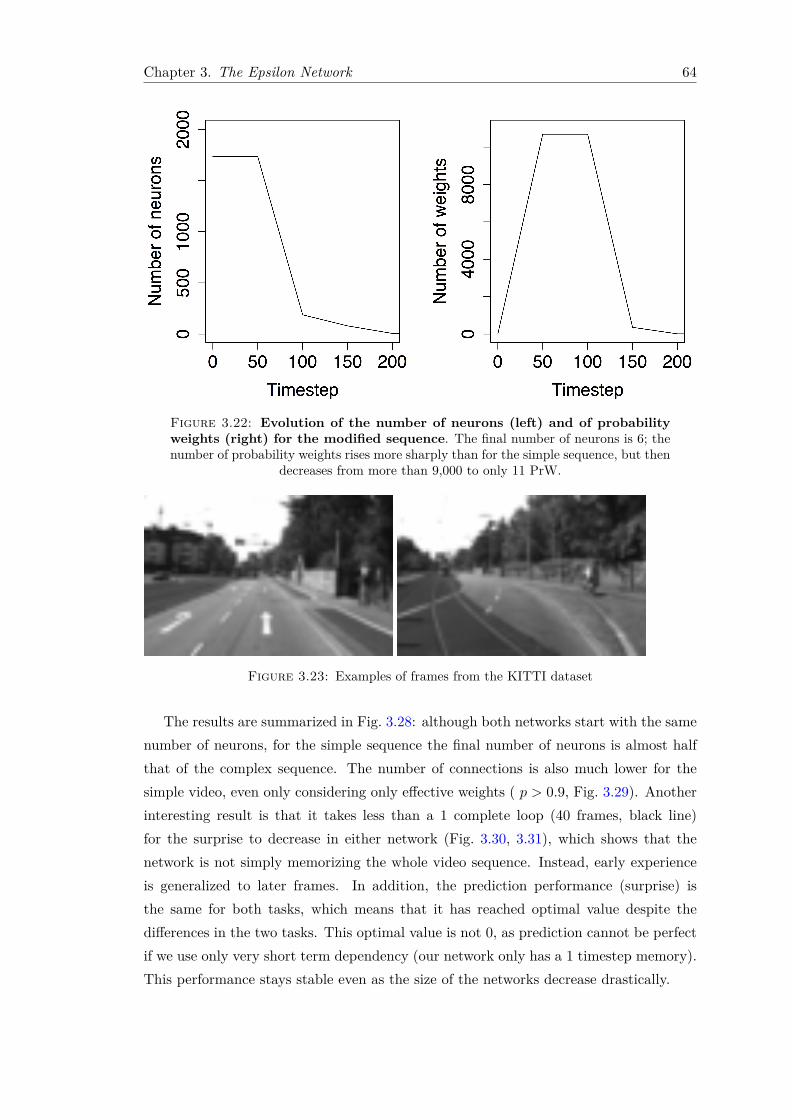
Chapter 3. The Epsilon Network 64
Figure 3.22: Evolution of the number of neurons (left) and of probabilityweights (right) for the modified sequence. The final number of neurons is 6; thenumber of probability weights rises more sharply than for the simple sequence, but then
decreases from more than 9,000 to only 11 PrW.
Figure 3.23: Examples of frames from the KITTI dataset
The results are summarized in Fig. 3.28: although both networks start with the samenumber of neurons, for the simple sequence the final number of neurons is almost halfthat of the complex sequence. The number of connections is also much lower for thesimple video, even only considering only effective weights ( p > 0.9, Fig. 3.29). Anotherinteresting result is that it takes less than a 1 complete loop (40 frames, black line)for the surprise to decrease in either network (Fig. 3.30, 3.31), which shows that thenetwork is not simply memorizing the whole video sequence. Instead, early experienceis generalized to later frames. In addition, the prediction performance (surprise) isthe same for both tasks, which means that it has reached optimal value despite thedifferences in the two tasks. This optimal value is not 0, as prediction cannot be perfectif we use only very short term dependency (our network only has a 1 timestep memory).This performance stays stable even as the size of the networks decrease drastically.

Chapter 3. The Epsilon Network 65
0 200 400 600 800
05
00
15
00
Timestep
Nu
mb
er
of n
eu
ron
s
No noiseWith noise
0 200 400 600 800
05
01
00
15
02
00
25
03
00
TimestepN
um
be
r o
f w
eig
hts
/ 1
03
Without noiseWith noise
Figure 3.24: Evolution of the number of neurons (left) and of predictionweights (right) on a clean video (blue lines) and a noisy version of the same video(red lines). The final results capture nicely the complexity induced by trying to predict
a noisy dataset.
0 200 400 600 800
05
01
00
15
02
00
25
03
00
Timestep
Nu
mb
er
of w
eig
hts
/ 1
03
Without noiseWith noise
0 200 400 600 800
05
01
00
15
02
00
25
03
00
Timestep
Nu
mb
er
of e
ffe
ctiv
e w
eig
hts
/ 1
03 Without noise
With noise
Figure 3.25: Evolution of the total number of prediction weights (left) andof the number of effective prediction weights (p > 0.9, right) on a clean video(blue lines) and a noisy version of the same video (red lines). There are more weightsin the network for the noisy video, but these additional weights have low predictivepower and the number of strong prediction weights is the same for the noisy and non
noisy video.

Chapter 3. The Epsilon Network 66
0 20 40 60 80 100
05
01
50
25
0
Timestep
Su
rpri
se
No noiseWith noise
Figure 3.26: Evolution of the surprise in the network with and withoutnoise. The value slowly decreases as the networks evolves. At t = 82 (black line), thevideo sequence starts a new loop which is a sudden and highly surprising event for the
network.
Figure 3.27: Frames from a simple sequence (2 characters play the accordionin almost periodic motion, static background) and a complex sequence (a
character rides a bicycle, the background changes)

Chapter 3. The Epsilon Network 67
0 200 400 600 800
05
00
10
00
20
00
Timestep
Nu
mb
er
of n
eu
ron
s
Simple videoComplex video
0 200 400 600 800
01
00
20
03
00
40
0Timestep
Nu
mb
er
of w
eig
hts
x 1
,00
0
Simple videoComplex video
Figure 3.28: Evolution of the number of neurons (left) and of weights (right)for the two experiments. Although both videos have the same number of frames,the number of neurons and connections is much higher for the complex video sequence.
0 200 400 600 800
02
04
06
08
01
00
Timestep
Nu
mb
er
of e
ffe
ctiv
e w
eig
hts
/ 1
03
Simple videoComplex video
Figure 3.29: Evolution of the number of effective weights (p > 0.9) for thesimple and complex videos. Unlike the results with or without noise, even whendiscounting the weak weights the complex video requires more weights than the simple
one. This is true complexity in the sense of Crutchfield.

Chapter 3. The Epsilon Network 68
0 200 400 600 800
01
00
30
0
Timestep
Su
rpri
se
Simple videoComplex video
Figure 3.30: Evolution of the surprise in the simple and complex task. Thesurprise decreases sharply at the beginning of either task, then stays stable at the
network optimizes its size.
0 50 100 150
05
01
00
15
02
00
25
03
00
Timestep
Su
rpri
se
Simple videoComplex video
Figure 3.31: Evolution of the surprise in the simple and complex task. Zoomon the first 150 steps shows small differences between the two time series, especially at
the first loop of the videos, the surprise is higher for the complex video.

Chapter 3. The Epsilon Network 69
Figure 3.32: Peak of new neurons indicating surprising events in the first150 frames. The first few timesteps the network has no knowledge, so everything is
surprising. After this naive period, all peaks correspond to significant events.
3.3.4 Surprising events
Due to its update rules, the network should be able to detect unexpected events andreact by creating new weights and new neurons. As a qualitative experiment, we letthe network (same parameters as the previous section) run on the Oswald cartoon andexamine the number of neurons, looking for peaks. As Fig. 3.32 and 3.32 show, each scenechange provokes a peak, and all other notable peaks correspond to reasonably surprisingevents, like sudden apparition of monsters or a fight scene. This simple analysis showsthat the network can be used to detect events of interest in a video.
3.3.5 Full model and long videos
We train the network on the entire Oswald video at a higher framerate (20 fps, 6644frames), with bigger images (72*54 pixels) and higher resolution (1 neuron per 2*2 pix-els). The network can create inhibitory weights. Every 50 timesteps, after the snappingprocedure, new modules are created as follows: all neurons from layer 4 or above are col-lected from all existing modules and serve as sensory input to a single common module.A video of the first learning timesteps can be found at https://youtu.be/yWNsiVHh_D8.
We compare the results for different snapping intervals: in Fig 3.34, 3.35 snapping isperformed every 50 steps, 100 steps, or never. The results show that not snapping gives

Chapter 3. The Epsilon Network 70
Figure 3.33: Peak of new neurons indicating surprising events in the first300 frames. The biggest peaks can be seen for scene changes, which are very much
unpredictable.
the best predictions, but requires a higher number of weights. This highlights one issueof this network: it is possible that 2 neurons have the exact same output predictionweights at early training time, but that these neurons would end up having differentoutput prediction weights after more training. If the neurons are compared too early,they will be fused together and there is no possibility to un-fuse them. For example, herethe video begins with black frames for several timesteps. When the network snaps, theneurons sensitive to white pixels have no output weights or only few output weights andthey are all fused together: the network becomes forever unable to perceive or predictseparately entire groups of white pixels. These bad predictions cause a higher number ofsurprised neurons; when trying to reduce this surprise the network paradoxically end upcreating more neurons than a networks that does not perform the snapping procedure.A brute force solution would be to find the ideal snapping frequency for a given dataset;a more elegant solution would be to detect when a neuron is the result of a too-earlyfusion (for example, the neuron becomes unable to make any correct prediction) anddivide it into as many neurons as needed when necessary.

Chapter 3. The Epsilon Network 71
0 2000 4000 6000 8000
05
10
15
20
Timestep
Mo
vin
g a
ve
rag
e M
SE
Snap interval 50: mean 4.01Snap interval 100: mean 3.71No snapping: mean 3.63
Figure 3.34: Mean Squared Error of the predictions for snapping every 50steps, 100 steps, or not snapping at all. We can see that the error gets smaller ifwe snap the network less often. This means that when fusing neurons together, a small
amount of information is lost that cannot be recovered.

Chapter 3. The Epsilon Network 72
0 2000 4000 6000 8000
05
00
01
00
00
15
00
02
00
00
25
00
03
00
00
Timestep
Nu
mb
er
of
ne
uro
ns
Snap interval 50Snap interval 100No snapping
Figure 3.35: Mean Number of neurons for snapping every 50 steps, 100steps, or not snapping at all. Snapping initially works as a method to reduce thenumber of neurons, but some information is lost by fusing neurons too early. Over-time this results in some bad predictions and number of neurons greater than without
snapping.

Chapter 3. The Epsilon Network 73
Table 3.1: Quantitative differences between the models
Model Neurons MSE Training time/set/epoch
PredNet 5.4x10¹⁰ 0.82 0.5 minute on 2 GPUS
ϵ-network 2.6x10³ 7.9 0.2 minute on 1 CPU
The ϵ-network has 107 times less neurons than PredNet but its final performance is10 times worse. It is also 2 times faster even if it is trained on a much less powerfularchitecture. On the other hand, the ϵ-network does not require an extensive and timeconsuming parameter search as does PredNet, as the same architecture can be used forany dataset.
3.3.6 Comparison with the state of the art: PredNet
The ϵ-network has different ambitions from the current Deep Learning (DL) boom,but how does it compare? As our model is in its infancy, we cannot expect to obtainextreme performance in terms of prediction, especially since we are more preoccupiedwith complexity modeling and online learning than with prediction performance andrepetition training. It is also not totally fair to compare the number of neurons usedby a DL network with the number of neurons of the ϵ-network, as DL networks runon architectures specifically conceived to support large amounts of neurons. Severaldozens of hours of training on GPU machines and hundred of repetitions per datasetare accepted as a trade off in exchange for extremely high performance.
Comparing parameters might be instructive if just to see how many orders of magni-tude are between the two models. In this experiment, we compare the ϵ-network with astate of the art DL network, PredNet [41]. We train the ϵ-network on the first 4 videosets in the KITTI dataset and compare the results on 2 other sets with the results ofPrednet. In terms of qualitative differences, it should be noted that in the paper Pred-Net was trained on the full 57 sets of KITTI, by batches of 10 frames of size 128x160pixels, for at least 150 epochs or more on GPUs. The ϵ-network is not meant to betrained by rote repetition, but to perform online learning. We train it on 108 framesof per video set, for 2 epochs; then we evaluate it on test data. The MSE cannot bedirectly compared with PredNet because the image format and pre-processing are dif-ferent, but we use the naive MSE (MSE of the current frame and the previous frame)of both models as a conversion factor and find the results in Table 3.1
Although the comparison is unfair due to differences in maturity of the models, goals,training protocol and amount of data, here is what we learn from this: the numberof neurons used by the ϵ-network is 7 orders of magnitude lower than the number of

Chapter 3. The Epsilon Network 74
neurons of PredNet (even extrapolating to 150 epochs and 57 video sets with the worsepossible growth conditions, our network should only reach 8x10⁶ neurons, likely less).The performance of PredNet is almost 2 orders of magnitudes greater than our model.This seems to hold true even in the first few epochs of PredNet training. Trainingtime is the same order of magnitude, but PredNet is highly optimized and runs on apowerful architecture, while the ϵ-network runs on a laptop PC (12 hours for PredNetfor 57 sets/50 epochs, 2 minutes for 4 sets/2 epochs for the ϵ-network). In addition, theparameters of PredNet (number of layers, number of channels, learning rate) have to beoptimized using heuristics, which multiplies the actual training time by as many timesas a new parameter has to be tested.
The conclusion of this experiment is that if someone was hesitating about whichmodel to use for which applications, we could give the following advice: if the applicationdepends on highly reliable predictions, the type of data is known in advance and thereis no limit on available computing power or training time, PredNet is the right choice.If the application tolerates moderately noisy predictions, requires to learn new inputson the fly in real time and with limited resources, the ϵ-network is the right choice.
3.4 Discussion
In this chapter, I presented the ϵ-network, a network that automatically adjusts its sizeto the complexity of a dataset while learning to predict its inputs. The network isinspired from Crutchfield’s work on the Epsilon Machine [2] and both models aim tomeasure complexity by predicting time series. One major difference is that the ϵ-networkperforms online learning, when the Epsilon Machine requires to know the entire datasetin advance. This makes the ϵ-network more suitable for tasks where real time processingis required and the data cannot be obtained beforehand.
Another major difference is that the Epsilon Machine operates on univariate timeseries and only has one node active at any given time, while the ϵ-network operateson multivariate time series and can have several neurons activated at the same time.This makes the ϵ-network more fit for tasks like video prediction or tasks with severalsimultaneous sources of data.
The last main difference with the Epsilon Machine is that the ϵ-network can adaptto noise automatically, without requiring to perform a parameter search to find thestructure adapted to a specific level of noise as the Epsilon Machine does. This meanswith my model, the same architecture can be used without any change to process a cleandataset or a dataset with an arbitrary level of noise. This is especially useful when wedo not know the data in advance.

Chapter 3. The Epsilon Network 75
There are other ways to adjust the size of a network during training [36]. GeneticAlgorithms are used to optimize the size of a neural network for a dataset, but unlikethe ϵ-network, they are not well suited for online learning. Genetic Algorithms requireto train several networks simultaneously for several generations in order to find the mostappropriate for the dataset. In contrast, the ϵ-network optimizes its size on the fly, it isnot necessary to train several networks simultaneously. It can adapt to the dataset inreal time.
Among the models of networks with self-adjusting size, the Growing Neural Gas [49]and Growing When Required [50] networks are models where the number of nodes isadjusted to match a spatial topology. There are two main differences with the ϵ-network.First, these models focus matching spatial structured – the networks literally grows tomatch the shape of a 2D or 3D object. The ϵ-network does not address the issue ofthe physical position of the neurons, but the temporal relationships between changinginputs. Indeed, except for the sensory neurons that are distributed over the 2D imageframe, the neurons in my model do not have spatial coordinates at all. Furthermore,the ϵ-network grows to match its output to a dynamical input that changed at everystep, while the Growing Neural Gas and Growing When Required networks are primarilyconcerned with inputs that stay static for many steps. In a sense, all models try to fitstatistical distributions, but the ϵ-network with its strong focus on prediction is moresuited to dynamical time series.
The main paradigm in neural network research is currently Deep Learning, and Iprovided a comparison of the ϵ-network with a Deep Learning network, PredNet [41].Both models perform predictive coding on video datasets, but in Deep Learning, thesize and structure of the networks do no change dynamically, and usually informs us notabout some property of the dataset but about how much computing power the researchteam had access to. Deep Learning networks are notoriously difficult to analyze andthe meaning of high performing topologies is an open issue. On the other hand, the ϵ-network’s main interest resides in the fact that its structure informs us about the natureof the data it was trained on. Not only how difficult the dataset is to predict, whichrepresents its complexity, but how much of this complexity is due to random noise andhow much of this complexity is intrinsic to the dataset.
In [37, 38, 39]), Friston presents Free Energy Minimization as a way to explain howprediction and inference can explain not only learning in the brain, but also an agent’sactions. As in this chapter, the focus is on prediction. In Friston’s work, agents learnand act to minimizing the value of surprise, which is related to the value of Free Energy.Similarly, in our work, surprise is also minimized by making the network learn. Our valueof surprise, as Friston’s, is not defined by the Shannon information where rare events are
Chapter 3. The Epsilon Network 76
surprising, but by the difference between prediction and input. This value of surpriseis used to increase the number of neurons, while comparing predictions allows us todecrease the number of neurons. This last points is relatively important for computers,but even more important for living organisms. Although we do not suggest that suchdrastic changes in brain density happen in animals, this network has a similarity withfamous cases of hydrocephaly (water in the brain) where humans retain complete abilitieswhile only a thin outer layer of brain cells remains alive.
For simple datasets, I showed that the ϵ-network can actually find the minimal au-tomaton representing this dataset, just as its inspiration the ϵ-machine[2] does. For morecomplex datasets, it is not obvious if the network will always find the minimal structurenecessary to reproduce the data stream. Yet as shown in the clean vs noisy datasetexperiment, the network has similar numbers of strong weights for datasets where theonly difference is the level of random noise. This suggests that the ϵ-network does infact capture the minimal structure representing a dataset. In addition, it adapts to noiseautomatically, while the epsilon machine of Crutchfield requires a parameter search todetermine which structure is more adapted to the level of noise in the data. This isanother advantage of our model.
I also show how the ϵ-network can be used to compare the complexity of two differentdatasets. The number of weights and neurons, even if we only consider the strongestvalues of weights, reflects the complexity of the datasets. As Crutchfield has said,periodic behaviors are predictable and therefore have lower complexity than aperiodicbehaviors, and the the ϵ-network capture this difference.
Despite not competing in terms of performance, when compared to PredNet, ourapproach shows interesting ratios: our network uses 107 times fewer neurons than Pred-Net, but only performs 10 times worse and also trains faster. In addition, it can performonline learning, which PredNet cannot; and it does not require hand tuning hundredsof parameters (number of layers, number of neurons).
To improve the ϵ-network, we could increase the capacity of the short term memory.Although computationally costly at the beginning of tasks, this might lead to evensmaller networks at the final stage of the learning task, as deeper temporal relationshipsare captured. For example, the modified falling ball task could theoretically be solvedwith only 3 neurons instead of 6 with a bigger short term memory. We could easily adaptpattern weights to detect temporal patterns. We are also in the process of implementingactions and proprioception in the network; early results suggest that this reduces thefinal size of the network for complex datasets, by allowing the network to recognize anobject even if it appears at different positions of the visual field.

Chapter 4
General Discussion
This thesis has presented two types of neural networks focusing on implementing action,prediction and classification in complex environments. The models address complexityas defined by Crutchfield (data produced by a mix of noise and periodicity) but alsocomplexity as defined by Weaver (data where several highly correlated part interacttogether). LSA faces noisy inputs as well as unreliability of the output’s effects, but stillmanages to map the inputs to the correct outputs. The ϵ-network faces purely periodicdata as well as data that is a mix of noise of periodicity, and data that is not purelyperiodic but results from highly correlated systems.
LSA allows a network to perform simple actions, mapping inputs and outputs insimple networks as we have seen in Section 2.3.2. LSA scales up to bigger networks of100 neurons despite high noise, as Section 2.4 demonstrates. These results were extendedto networks of 3000 neurons in [33]. It therefore offers a convincing explanation to theexisting results of biological experiments of Shahaf, and our explanation is backed upby experimental results. I also demonstrated the necessity of burst suppression, whichwas not addressed by Shahaf, in Section 2.4.1. LSA is also robust to unreliability ofthe output’s effects, as the embodied application in Section 2.6 shows. LSA is basedon biological data, and Chapter 2 as a whole updates our understanding of low levelquestions about the biological implementation of prediction, explains so far unexplainedbiological results and offers a way to develop more applications for biological or simulatedspiking networks. What LSA identifies as noise is entirely dependent on whether thenetwork’s actions can manipulate the value of its sensory inputs: internal noise cannotbe manipulated and is ignored.
In Section 3.17 I showed how the ϵ-network can extract the minimal probabilistic au-tomaton of a multivariate time series. The experiment demonstrated how the ϵ-networkcan replicate the functionality of the epsilon machine of Crutchfield, despite having a
77

Chapter 4: Messages from this thesis and future work 78
different implementation. Because our implementation is so different and we performonline learning on multivariate time series, there could be a concern that the networkdoes not do as well as an epsilon machine, but this experiment on a toy dataset demon-strates the validity of our model. The ϵ-network is able to adapt its topology to maintainperformance despite random noise, and to separate signal from noise; it can also adaptto true complexity as shown in Section 3.3.2. It is based on more speculative, high-level hypotheses than LSA, but offers many advantages over the existing ϵ-Machines:optimized online learning instead of offline building of the machine, processing of multi-variate streams instead of univariate streams, and automatic adaptation to noise insteadof parameter search. As a whole, Chapter 3 proposes answers to high level questionsabout intelligence, such as how does classification emerges from prediction, the relation-ship between the the unconscious and memory, and the relationship between surpriseand prediction:
• Objects belong to the same class if they allow similar predictions
• Higher level classes block the access of their subclasses to short term memory
• Surprise is used as a measure of error to improve prediction performance.
With LSA, learning consists in adapting the complexity of the agent’s behavior to itsempowerment, defined by Polani as “how much influence and control an agent has overthe world it can perceive” [51]. In Polani’s research, agents act as to always maximizeempowerment, but empowerment is known in advance. However, with LSA, it is empow-erment itself that is learned by the network. Everything that cannot be manipulated,including random external input, is irrelevant to the network’s goal and considered asnoise.
With the ϵ-network, learning consists in predicting of an input stream. The EpsilonMachine of Crutchfield has the same goal. However, unlike the Epsilon Machine, theϵ-network does not require to know the data in advance. This makes the the ϵ-networkespecially suited to online learning.
In this way, my research can be linked to existing work about predictive coding,especially the work of Friston and al. on Free Energy Minimisation [37, 38, 39]. Fristonalso speculates about how learning can happen in agents in the real world and howprediction can guide action. Nevertheless, because of its extreme complexity, there havebeen few complete implementations of Friston’s ideas. Especially, implementation isfocused on agent that already have a perfect model of the world. My model focuses onlearning and building this model of the world, so that the agent does not have to knowanything at the start of the experiment.

Chapter 4: Messages from this thesis and future work 79
Deep Learning networks can also be used for predictive coding and can have excellentperformance. However, their structure is fixed and they cannot perform online learningeither. The ϵ-network not only performs prediction of an input stream, but it adjust itsinternal structure to the complexity of the input data. This allows us to draw conclusionsabout the data just by looking at the structure of this network.
Although drastic volume changes in the mammal brain are not commonplace, theϵ-network also offers cues into how can humans lose neurons during development whileat the same time becoming more and more performant; why in some pathological casessomeone can lose 90% of the volume of their brain and still behave appropriately indaily life [52]; and how some bird and mammal species can drastically reduce and growback their number of neurons depending on the season while still being able to exhibitnormal behavior [53, 54, 55].
The ϵ-network can also be viewed as an implementation of the Interface Theory ofPerception [4]. In his paper, Hoffman says that an organism does not have to perceive theworld as it is or as accurately as possible, but instead perceive the world as accuratelyas is necessary and not more accurately than necessary. The ϵ-network starts withas much accuracy as its sensors allow, but as it learns, inputs are classified accordingto the similarity of the prediction they offer. Once snapped together, inputs becomeindistinguishable. This is the definition of “perceiving the world as accurately as isnecessary and not more” as Hoffman presented it.
The two networks that I presented change their topology to minimize different quan-tities: LSA seeks behaviors that can reduce external stimulation, while the ϵ-networkreduces the amount of surprise caused by external inputs. It is possible to integrateboth approaches in one single framework: if only unpredicted inputs cause stimulation,LSA becomes a low level implementation of the ϵ-network, but the notion of action islost. We can go further and define stimulation as “unmanipulable inputs”: can theagent have an effect on some of the input values, and if yes, can this effect be predicted?If the effect of the agent’s actions on the input stream cannot be predicted, this un-predictability becomes stimulation. In this case, we get the best of both LSA and theϵ-network: the agent is motivated to act when it cannot predict the results of its ownactions, until its predictions become accurate. Such an agent would display a form ofintrinsic motivation that depends not simply on an assigned task or on a reward signal,but on its own knowledge of the environment and understanding of its own abilities.“Can I predict what happens if I push this button? If not, I have to push it and learnwhat can happen.” Such an agent would learn not only a model of its environment, buta model of its empowerment in that environment; and that model would have just theright amount of complexity to map the agent’s abilities to the world it lives in.

Chapter 4: Messages from this thesis and future work 80
A topic that will be of particular interest is the relationship between episodic memo-ries and predictive coding. The consensus about episodic memory is that it is not“stored”somewhere like we would store a video tape (see [56]), but each memory is reconstructedeach time that we want to access it. Memories are modified each time that they arereconstructed, according to what we think “probably happened” at that time. In otherwords, predictions play a role when we remember past episodes of our life. Since ourpredictions also change depending on what we learn from day to day, this could be thereal source for erroneous and false memories. Indeed, early work with the ϵ-network sug-gests that when episodic memories are reconstructed by generating video frames frompartial input enhanced by strong prediction weights, false memories can be implantedin the network using the same techniques of suggestion that are used on humans: cre-ating associations between past objects and new stimuli, mentally rehearsing the falsememory.
Prediction is also theorized to be the engine of the “System 1” identified by thebehavioral economist Daniel Kahneman in his book [57]: System One directs humanbeings’ automatic actions and reactions, intuitions, and every decision that relies onspeed rather than accuracy. System 2 is in charge of deliberate decision making, decisionsthat take time and require precision. Switching from System 1 to System 2 during adecision process happens when the expectations of System 1 about the world are sowrong that inputs cannot be processed automatically anymore. In terms of ϵ-network,System 1 would be an automatic process treating strong prediction weights as if theywere real inputs, running in quasi-closed loop without needing to use the Short TermMemory. System 1 would make processing faster by omitting the whole bottom-upclassification and top-down trickle of predictions to lower modules. System 2 would be aprocess waiting for actual environmental inputs to reach the STM and classifying theseinputs before making the next predictions, and using these predictions to take decisions.This aligns nicely with Kahneman’s observation that the processes of System 1 do notstay in memory, and when taking decisions in this form of autopilot, humans cannotexplain why they took these decisions. In the ϵ-network, the STM is only used to updateweights, and is not necessary to generate predictions from existing weights. System 1does not need to use the memory, and so its decision process remains unconscious andinexplicable by the conscious agent itself.
Beyond the speculative and explanatory aspects of my research, existing applicationsexist as future work. Both LSA-based networks and the ϵ-network put emphasis onlow computational cost: in combination, they could improve the chances of developingapplications that depend on prediction in everyday devices: object tracking, self local-ization... For higher level applications, the ϵ-network’s ability to classify time series canbe used for identifying entities in swarms and other highly dynamic systems. On the

Chapter 4: Messages from this thesis and future work 81
contrary, its inability to predict the dynamics of a single entity could be used to detectagency: if an object’s trajectory cannot be predicted only from its environment’s history,maybe that trajectory is controlled from internal parameters akin to agency.
Many functions of the brain seem to happen independently of external rewards, andfor now the model learns without reward signal. However, goal directed behavior isan important part of the life of biological organisms. We are in the process of imple-menting reinforcement learning for reward-based behaviors. Because the network makespredictions, it can also predict the activation of reward neurons, and therefore choosethe actions that lead to higher activation of these reward neurons. The reward neuronsactivation can be decided by implementing simple policies, as in standard reinforcementlearning frameworks. The ϵ-network can have many interesting applications, and I planto work more on the integration of action and embodiment.

Acknowledgements
All my gratitude goes to the members and honorary members of the Ikegami Lab forthe hours of discussion that ultimately lead to this thesis: Norihiro Maruyama, AtsushiMasumori, Martin Biehl, Olaf Witowski, Nathaniel Virgo, Hiroki Kojima, Itsuki Doi,Julien Hubert. I am thankful to Ikegami Takashi for his support during my research,and to Nicholas Guttenberg for joining our discussions despite the distance.
Special thanks to the dedicated readers who volunteered to comment on my thesis: PaulHarland, Rafaela Libano, Rodolfo Cruz-Silva, Eric Sinapayen, Marie-Noelle Sinapayen,Sean Aubin, Julien Hubert.
82

Bibliography
[1] Warren Weaver. “Science and complexity”. In: Facets of systems science. Springer,1947, pp. 449–456.
[2] J. P. Crutchfield and K. Young. “Inferring Statistical Complexity”. In: PhysicalReview Letters 63.2 (1989), pp. 105–108.
[3] Jakob Von Uexküll. “A stroll through the worlds of animals and men: A picturebook of invisible worlds”. In: Semiotica 89.4 (1957), pp. 319–391.
[4] Donald D Hoffman, Manish Singh, and Chetan Prakash. “The interface theory ofperception”. In: Psychonomic bulletin & review 22.6 (2015), pp. 1480–1506.
[5] Charles Duhigg. The Power of Habit. Penguin Books Random House, 2012.
[6] Goded Shahaf and Shimon Marom. “Learning in networks of cortical neurons”.In: The Journal of Neuroscience 21.22 (2001), pp. 8782–8788.
[7] Shimon Marom and Goded Shahaf. “Development, learning and memory in largerandom networks of cortical neurons: lessons beyond anatomy”. In: Quarterly re-views of biophysics 35.01 (2002), pp. 63–87.
[8] Clark Leonard Hull. Principles of behavior: an introduction to behavior theory.Appleton-Century, 1943.
[9] Edwin R Guthrie. “Psychological facts and psychological theory.” In: PsychologicalBulletin 43.1 (1946), pp. 1–20.
[10] Eugene M Izhikevich. “Solving the distal reward problem through linkage of STDPand dopamine signaling”. In: Cerebral cortex 17.10 (2007), pp. 2443–2452.
[11] George L Chadderdon, Samuel A Neymotin, Cliff C Kerr, and William W Lytton.“Reinforcement learning of targeted movement in a spiking neuronal model ofmotor cortex”. In: PloS one 7.10 (2012), e47251.
[12] Samuel A Neymotin, George L Chadderdon, Cliff C Kerr, Joseph T Francis, andWilliam W Lytton. “Reinforcement learning of two-joint virtual arm reaching ina computer model of sensorimotor cortex”. In: Neural computation 25.12 (2013),pp. 3263–3293.
83

Bibliography 84
[13] Lana Sinapayen, Atsushi Masumori, Nathaniel Virgo, and Takashi Ikegami. “Learn-ing by Stimulation Avoidance as a primary principle of spiking neural networksdynamics.” In: 13th European Conference on Artificial Life (ECAL 2015) (2015),pp. 175–182.
[14] Atsushi Masumori, Norihiro Maruyama, Lana Sinapayen, Takeshi Mita, Urs Frey,Douglas Bakkum, Hirokazu Takahashi, and Takashi Ikegami. “Emergence of sense-making behavior by the Stimulus Avoidance Principle: Experiments on a robotbehavior controlled by cultured neuronal cells”. In: 13th European Conference onArtificial Life (ECAL 2015) (2015), pp. 373–380.
[15] Donald O Hebb. The organization of behavior. Wiley, New York, 1949.
[16] John Lisman and Nelson Spruston. “Questions about STDP as a general model ofsynaptic plasticity”. In: Frontiers in Synaptic Neuroscience 2 (2010), p. 140.
[17] Natalia Caporale and Yang Dan. “Spike timing-dependent plasticity: a Hebbianlearning rule”. In: Annu. Rev. Neurosci. 31 (2008), pp. 25–46.
[18] Yang Dan and Mu-Ming Poo. “Spike timing-dependent plasticity: from synapse toperception”. In: Physiological reviews 86.3 (2006), pp. 1033–1048.
[19] Sen Song, Kenneth D Miller, and Larry F Abbott. “Competitive Hebbian learningthrough spike-timing-dependent synaptic plasticity”. In: Nature neuroscience 3.9(2000), pp. 919–926.
[20] Stijn Cassenaer and Gilles Laurent. “Hebbian STDP in mushroom bodies facili-tates the synchronous flow of olfactory information in locusts”. In: Nature 448.7154(2007), pp. 709–713.
[21] Vincent Jacob, Daniel J Brasier, Irina Erchova, Dan Feldman, and Daniel E Shulz.“Spike timing-dependent synaptic depression in the in vivo barrel cortex of therat”. In: The Journal of Neuroscience 27.6 (2007), pp. 1271–1284.
[22] Yu-Xi Fu, Kaj Djupsund, Hongfeng Gao, Benjamin Hayden, Kai Shen, and YangDan. “Temporal specificity in the cortical plasticity of visual space representation”.In: Science 296.5575 (2002), pp. 1999–2003.
[23] Sven Schuett, Tobias Bonhoeffer, and Mark Hübener. “Pairing-induced changes oforientation maps in cat visual cortex”. In: Neuron 32.2 (2001), pp. 325–337.
[24] Daniel Bush, Andrew Philippides, Phil Husbands, and Michael O’Shea. “Reconcil-ing the STDP and BCM models of synaptic plasticity in a spiking recurrent neuralnetwork”. In: Neural computation 22.8 (2010), pp. 2059–2085.
[25] Eugene M Izhikevich et al. “Simple model of spiking neurons”. In: IEEE Transac-tions on neural networks 14.6 (2003), pp. 1569–1572.

Bibliography 85
[26] Eugene M Izhikevich. “Which model to use for cortical spiking neurons?” In: IEEEtransactions on neural networks 15.5 (2004), pp. 1063–1070.
[27] Douglas L Meinecke and Alan Peters. “GABA immunoreactive neurons in ratvisual cortex”. In: Journal of Comparative Neurology 261.3 (1987), pp. 388–404.
[28] Romain Brette, Michelle Rudolph, Ted Carnevale, Michael Hines, David Beeman,James M Bower, Markus Diesmann, Abigail Morrison, Philip H Goodman, Freder-ick C Harris Jr, et al. “Simulation of networks of spiking neurons: a review of toolsand strategies”. In: Journal of computational neuroscience 23.3 (2007), pp. 349–398.
[29] Orit Shefi, Ido Golding, Ronen Segev, Eshel Ben-Jacob, and Amir Ayali. “Mor-phological characterization of in vitro neuronal networks”. In: Physical Review E66.2 (2002), p. 021905.
[30] Daniel A Wagenaar, Radhika Madhavan, Jerome Pine, and Steve M Potter. “Con-trolling bursting in cortical cultures with closed-loop multi-electrode stimulation”.In: The Journal of neuroscience 25.3 (2005), pp. 680–688.
[31] Nicolas Brunel. “Dynamics of sparsely connected networks of excitatory and in-hibitory spiking neurons”. In: Journal of computational neuroscience 8.3 (2000),pp. 183–208.
[32] Gianluigi Mongillo, Omri Barak, and Misha Tsodyks. “Synaptic theory of workingmemory”. In: Science 319.5869 (2008), pp. 1543–1546.
[33] Atsushi Masumori, Lana Sinapayen, and Takashi Ikegami. “Learning by Stimula-tion Avoidance Scales to Large Neural Networks”. In: 14th European Conferenceon Artificial Life (ECAL 2017) (2017), pp. 275–282.
[34] Karl Friston. “The free-energy principle: a unified brain theory?” In: Nature Re-views Neuroscience 11.2 (2010), pp. 127–138.
[35] Daniel E Feldman. “The spike-timing dependence of plasticity”. In: Neuron 75.4(2012), pp. 556–571.
[36] M. Attik, L. Bougrain, and F. Alexandre. “Neural network topology optimization”.In: Artificial Neural Networks: Formal Models and Their Applications–ICANN2005 (2005), pp. 748–748.
[37] K. Friston. “A theory of cortical responses”. In: Philosophical Transactions of theRoyal Society of London B: Biological Sciences 360.1456 (2005), pp. 815–836.
[38] K. Friston and S. Kiebel. “Predictive coding under the free-energy principle”. In:Philosophical Transactions of the Royal Society B: Biological Sciences 364.1521(2009), pp. 1211–1221.

Bibliography 86
[39] K. Friston. “The free-energy principle: a rough guide to the brain?” In: Trends incognitive sciences 13.7 (2009), pp. 293–301.
[40] W. Lotter, G. Kreiman, and D. Cox. “Unsupervised learning of visual structureusing predictive generative networks”. In: arXiv preprint arXiv:1511.06380 (2015).
[41] W. Lotter, G. Kreiman, and D. Cox. “Deep predictive coding networks for videoprediction and unsupervised learning”. In: arXiv preprint arXiv:1605.08104 (2016).
[42] J. Hawkins and S. Blakeslee. On Intelligence. Times Books, 2004.
[43] S. J. Garalevicius. “Memory-Prediction Framework for Pattern Recognition: Per-formance and Suitability of the Bayesian Model of Visual Cortex.” In: FLAIRSConference. 2007, pp. 92–97.
[44] M. Bundzel and S. Hashimoto. “Object identification in dynamic images basedon the memory-prediction theory of brain function”. In: Journal of IntelligentLearning Systems and Applications 2.04 (2010), p. 212.
[45] David Rawlinson and Gideon Kowadlo. “Generating adaptive behaviour within amemory-prediction framework”. In: PloS one 7.1 (2012), e29264.
[46] P. Baldi and L. Itti. “Of bits and wows: a Bayesian theory of surprise with appli-cations to attention”. In: Neural Networks 23.5 (2010), pp. 649–666.
[47] A Geiger, P. Lenz, C Stiller, and R. Urtasun. “Vision meets robotics: The KITTIdataset”. In: International Journal of Robotics Research (2013).
[48] Accessed: 2017-04-12 W. Lantz and B. Nolan. Mechanical Man, Oswald theLucky Rabbit series. https://www.youtube.com/watch?v=gOkXItHRnsg. 1932.
[49] Bernd Fritzke. “A growing neural gas network learns topologies”. In: Advances inneural information processing systems. 1995, pp. 625–632.
[50] Stephen Marsland, Jonathan Shapiro, and Ulrich Nehmzow. “A self-organisingnetwork that grows when required”. In: Neural networks 15.8-9 (2002), pp. 1041–1058.
[51] Christoph Salge, Cornelius Glackin, and Daniel Polani. “Empowerment–an intro-duction”. In: Guided Self-Organization: Inception. Springer, 2014, pp. 67–114.
[52] Lionel Feuillet, Henry Dufour, and Jean Pelletier. “Brain of a white-collar worker.”In: Lancet (London, England) 370.9583 (2007), p. 262.
[53] Geert De Groof, Marleen Verhoye, Colline Poirier, Alexander Leemans, MarcelEens, Veerle M Darras, and Annemie Van der Linden. “Structural changes betweenseasons in the songbird auditory forebrain”. In: Journal of Neuroscience 29.43(2009), pp. 13557–13565.
[54] Anthony D Tramontin and Eliot A Brenowitz. “Seasonal plasticity in the adultbrain”. In: Trends in neurosciences 23.6 (2000), pp. 251–258.

Bibliography 87
[55] Javier Lázaro, Dina KN Dechmann, Scott LaPoint, Martin Wikelski, and MoritzHertel. “Profound reversible seasonal changes of individual skull size in a mam-mal”. In: Current Biology 27.20 (2017), R1106–R1107.
[56] Julia Shaw. The Memory Illusion. Penguin Random House Books, 2016.
[57] Daniel Kahneman. Thinking, Fast and slow. Penguin Books, 2011.

Publications
[1] Referred, Published Lana Sinapayen, Atsushi Masumori, Nathaniel Virgo, andTakashi Ikegami. “Online Fitting of Computational Cost to Environmental Com-plexity: Predictive Coding with the epsilon-network”. In: 14th European Conferenceon Artificial Life (ECAL 2017) (2017).
[2] Referred, Published Lana Sinapayen and Takashi Ikegami. “Learning by stim-ulation avoidance: A principle to control spiking neural networks dynamics”. In:PloS one 12.2 (2017), e0170388.
[3] Referred, Published Atsushi Masumori, Lana Sinapayen, and Takashi Ikegami.“Learning by Stimulation Avoidance Scales to Large Neural Networks”. In: 14thEuropean Conference on Artificial Life (ECAL 2017) (2017).
[4] Non-referred, Published Lana Sinapayen and Takashi Ikegami. “Video Com-pression with a Predictive Neural Network”. In: Proceedings of the conference ofJapanese Society for Artificial Intelligence. 2017.
[5] Non-referred, Published 升森 敦⼠, Lana Sinapayen, and 池上 ⾼志. “GACSオートマトンのシミュレーション”. In: Proceedings of the conference of JapaneseSociety for Artificial Intelligence. 2017.
[6] Non-referred, Published L Sinapayen and T Ikegami. “A New Principle toShape Spiking Neural Networks Dynamics: Learning by Stimulation Avoidance”.In: Meeting Abstracts of the Physical Society of Japan 71.1. The Physical Societyof Japan. 2016, p. 3038.
[7] Non-referred, Published ⼩島 ⼤樹, ⼟井 樹, Lana Sinapayen, and 池上 ⾼志.“DCGAN を⽤いた記憶と表象のモデル”. In: Proceedings of the conference ofJapanese Society for Artificial Intelligence. 2016, pp. 2747–2747.
[8] Non-referred, Published Caleb Scharf, Nathaniel Virgo, H James Cleaves,Masashi Aono, Nathanael Aubert-Kato, Arsev Aydinoglu, Ana Barahona, LauraM Barge, Steven A Benner, Martin Biehl, Ramon Brasser, Christopher J. Butch,Kuhan Chandru, Leroy Cronin, Sebastian Danielache, Jakob Fischer, John Hern-lund, Piet Hut, Takashi Ikegami, Jun Kimura, Kensei Kobayashi, Carlos Mariscal,McGlynn Shawn, Brice Menard, Norman Packard, Robert Pascal, Juli Pereto,Sudha Rajamani, Lana Sinapayen, Eric Smith, Christopher Switzer, Ken Takai,
88

Bibliography 89
Feng Tian, Yuichiro Ueno, Mary Voytek, Olaf Witkowski, and Hikaru Yabuta. “Astrategy for origins of life research”. In: Journal of Astrobiology. 2015, pp. 1031–1042.
[9] Referred, Published Lana Sinapayen, Atsushi Masumori, Nathaniel Virgo, andTakashi Ikegami. “Learning by Stimulation Avoidance as a primary principle ofspiking neural networks dynamics.” In: 13th European Conference on ArtificialLife (ECAL 2015) (2015), pp. 175–182.
[10] Referred, Published Atsushi Masumori, Norihiro Maruyama, Lana Sinapayen,Takeshi Mita, Urs Frey, Douglas Bakkum, Hirokazu Takahashi, and Takashi Ikegami.“Emergence of sense-making behavior by the Stimulus Avoidance Principle: Ex-periments on a robot behavior controlled by cultured neuronal cells”. In: 13thEuropean Conference on Artificial Life (ECAL 2015) (2015), pp. 373–380.