an overview of convolutional neural network architectures ... · an overview of convolutional...
TRANSCRIPT

An Overview of Convolutional
Neural Network Architectures for
Deep Learning
John Murphy1
Microway, Inc.
Fall 2016

Abstract
Since AlexNet was developed and applied to the ImageNet classi�cation competitionin 2012 [1], the quantity of research on convolutional networks for deep learning appli-cations has increased remarkably. In 2015, the top 5 classi�cation error was reducedto 3.57%, with Microsoft's Residual Network [2]. The previous top 5 classi�cationerror was 6.67%, achieved by GoogLeNet [3]. In recent years, new arti�cial neuralnetwork architectures have been developed which improve upon previous architectures.Speci�cally, these are the inception modules in GoogLeNet, and residual networks, inMicrosoft's ResNet [2]. Here we will examine convolutional neural networks (convnets)for image recognition, and then provide an explanation for their architecture. The roleof various convnet hyperparameters will be examined. The question of how to correctlysize a neural network, in terms of the number of layers, and layer size, for example,will be considered. An example for determining GPU memory required for training ade�ned network architecture is presented. The training method of backpropagationwill be discussed in the context of past and recent developments which have improvedtraining e�ectiveness. Other techniques and considerations related to network training,such as choosing an activation function, and proper weight initialization, are discussedbrie�y. Finally, recent developments in convnet architecture are reviewed.
2

Contents
1 Introduction 5
2 Convnet Architecture 5
3 Filter Convolution 73.1 Filter Size . . . . . . . . . . . . . . . . . . . . . . . . . . . . . . . . . . . 73.2 Padding . . . . . . . . . . . . . . . . . . . . . . . . . . . . . . . . . . . . 73.3 Stride . . . . . . . . . . . . . . . . . . . . . . . . . . . . . . . . . . . . . . 83.4 Convolution Arithmetic . . . . . . . . . . . . . . . . . . . . . . . . . . . . 83.5 Pooling . . . . . . . . . . . . . . . . . . . . . . . . . . . . . . . . . . . . . 9
4 Network Design Questions 10
5 Convnet Training 105.1 Optimization Methods . . . . . . . . . . . . . . . . . . . . . . . . . . . . . 115.2 Regularization . . . . . . . . . . . . . . . . . . . . . . . . . . . . . . . . . 125.3 Network Weight Initialization . . . . . . . . . . . . . . . . . . . . . . . . . 125.4 Dropout . . . . . . . . . . . . . . . . . . . . . . . . . . . . . . . . . . . . 125.5 Image Data Augmentation . . . . . . . . . . . . . . . . . . . . . . . . . . . 135.6 Activation Functions . . . . . . . . . . . . . . . . . . . . . . . . . . . . . . 13
6 Determining Compute Resources Required for a Convnet 146.1 Parameter Counting . . . . . . . . . . . . . . . . . . . . . . . . . . . . . . 146.2 Memory Requirement . . . . . . . . . . . . . . . . . . . . . . . . . . . . . 156.3 Similar Network, with More Layers, and Stride 1 . . . . . . . . . . . . . . . 166.4 Computational Requirement . . . . . . . . . . . . . . . . . . . . . . . . . . 17
7 Newer Developments 187.1 Inception Modules . . . . . . . . . . . . . . . . . . . . . . . . . . . . . . . 187.2 Residual Networks . . . . . . . . . . . . . . . . . . . . . . . . . . . . . . . 18
8 Conclusion 19
9 Acknowledgements 20
3

List of Figures
1 A Malamute can, in many instances, not be immediately discernable from aSiberian Husky (Malamute is on right). . . . . . . . . . . . . . . . . . . . . 5
2 A convolutional neural network with max pool layers. Here, max poolingchooses the highest pixel value in a 2×2 patch translated in increments of 2pixels. This reduced the number of pixels by a factor of 4. See the sectionbelow on Pooling for more details on max pooling). . . . . . . . . . . . . . 6
3 Computing the output values of a discrete convolution. For the subplots, darkblue squares indicate neurons in the �lter region. Dark green squares indicatethe output neuron for which the total input activation is computed. . . . . . 7
4 With zero padding, the e�ect of output size reduction is counteracted tomaintain the input size at the output. . . . . . . . . . . . . . . . . . . . . . 8
5 Convolution with zero padding and stride > 1. Only the �st three subplotsare shown here. Padding is of depth 1, stride is 2, and �lter size is 3×3 . . . 8
6 This is an example of computing the maxpool output at three 3×3 patchlocations on an activation layer. Max pooling is applied on 3×3 patches.Max pooling increases the intensity of pixels upon pooling, since only themaximum intensity pixel was chosen from each pooled area. . . . . . . . . . 9
7 A convolutional neural network with max pool layers replaced by convolutionlayers having stride 2. . . . . . . . . . . . . . . . . . . . . . . . . . . . . . 14
List of Tables
1 Because of the stride of 2, the activation layers become reduced approximatelyby a factor of 2 after every convolution. Max pooling is becoming replacedby convnets having stride > 1. . . . . . . . . . . . . . . . . . . . . . . . . . 15
2 Number of activations present in each layer, and the memory required forsingle precision activation values. Notice that network activations occupymuch more memory toward the input. Multiply the memory requirement bytwo to also account for the memory needed to cache gradients during theforward pass, for later backpropagation. . . . . . . . . . . . . . . . . . . . . 16
3 Number of parameters required for each network layer, and the memory re-quired for single precision parameters. The memory requirements assume thateach parameter is 4 bytes, or a single precision �oating point number. . . . . 17
4
1 Introduction
Research in arti�cial neural networks began almost 80 years ago [4]. For many years, therewas no widely accepted biological model for visual neural networks, until experimental workelucidated the structure and function of the mammalian visual cortex [5]. Thereafter, the-oreticians constructed models bearing similarity to biological neural networks [6]. Whiletheoretical progress continued with the development of methods for training convnets, therewas no practical method for training large networks yet in place. With the developmentof LeNet, by Yann LeCunn,et al., the �rst practical convnet was deployed for recognizinghand-written digits on bank checks [7]. This paper will discuss some of the major networkparameters and learning techniques related to convnets.
2 Convnet Architecture
Since AlexNet was demonstrated, in 2012, to outperform all other methods for visual clas-si�cation, convnets began to attract great attention from the research community[1]. Byperforming matrix operations in parallel on Graphical Processing Units (GPUs) in consumerdesktop computers, it became possible to train larger networks in order to classify across alarge number of classes, taken from ImageNet [8]. Since AlexNet, research activity in DeepLearning has increased remarkably.Large neural networks have the ability to emulate the behavior of arbitrary, complex, non-
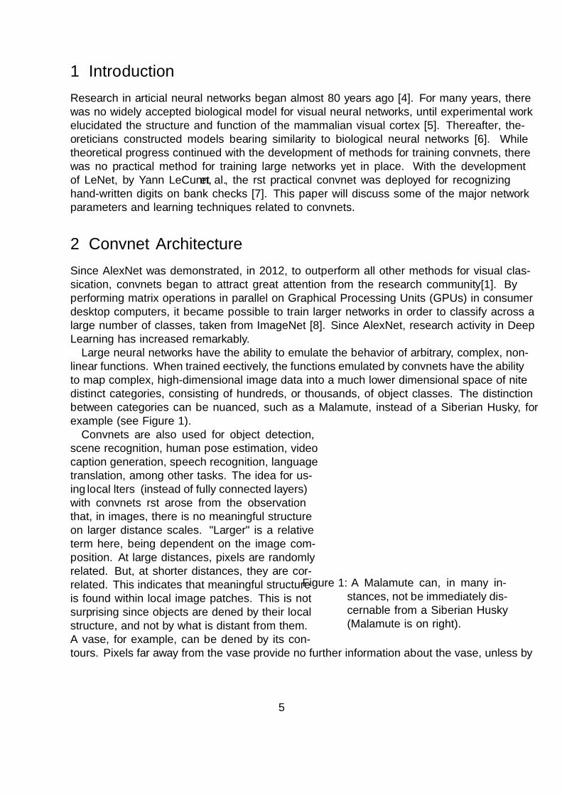
linear functions. When trained e�ectively, the functions emulated by convnets have the abilityto map complex, high-dimensional image data into a much lower dimensional space of �nitedistinct categories, consisting of hundreds, or thousands, of object classes. The distinctionbetween categories can be nuanced, such as a Malamute, instead of a Siberian Husky, forexample (see Figure 1).
Figure 1: A Malamute can, in many in-stances, not be immediately dis-cernable from a Siberian Husky(Malamute is on right).
Convnets are also used for object detection,scene recognition, human pose estimation, videocaption generation, speech recognition, languagetranslation, among other tasks. The idea for us-ing local �lters (instead of fully connected layers)with convnets �rst arose from the observationthat, in images, there is no meaningful structureon larger distance scales. "Larger" is a relativeterm here, being dependent on the image com-position. At large distances, pixels are randomlyrelated. But, at shorter distances, they are cor-related. This indicates that meaningful structureis found within local image patches. This is notsurprising since objects are de�ned by their localstructure, and not by what is distant from them.A vase, for example, can be de�ned by its con-tours. Pixels far away from the vase provide no further information about the vase, unless by
5
coincidence, a vase, for example, is always positioned adjacent to a small cube. With suchan image set, an image classi�er trained to recognize vases may also use elements of thecube to determine whether a vase is in the image.In fact, before training, it is not clear what sort of features a network will select in order
to improve recognition. One network trained by [9], for example, could recognize race cars,in part, by developing detectors for the text content of advertisement decals stuck to thesides of them- not necessarily something one would immediately associate with a car. Butsince it was a distinguishing feature of race cars, the network learned to recognize the textin advertisements, and then use this feature, in a distributed representation, to activate thenetwork output indicating race car category, and not some other type of car. Similar sortsof di�erences are used by networks to sort out recognition of similar breeds of dogs (such asSiberian Huskies and Malamutes).The structural information contained in local regions of images motivated the use of
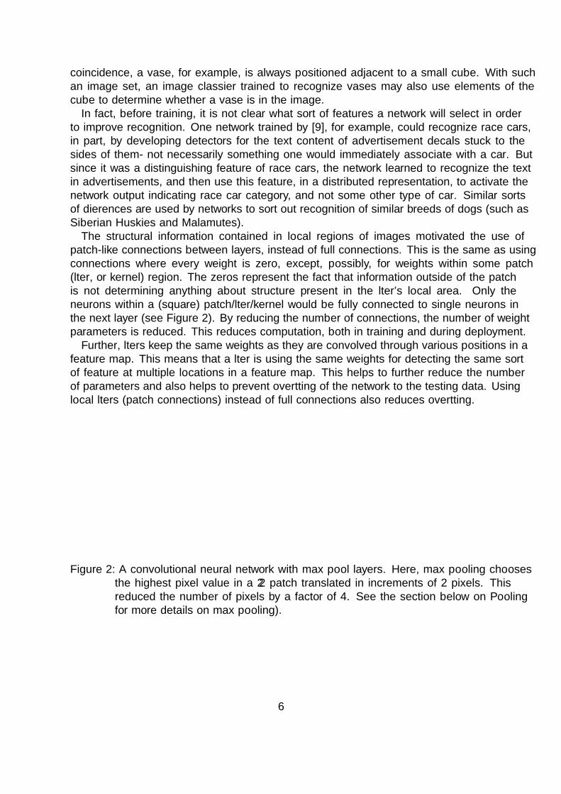
patch-like connections between layers, instead of full connections. This is the same as usingconnections where every weight is zero, except, possibly, for weights within some patch(�lter, or kernel) region. The zeros represent the fact that information outside of the patchis not determining anything about structure present in the �lter's local area. Only theneurons within a (square) patch/�lter/kernel would be fully connected to single neurons inthe next layer (see Figure 2). By reducing the number of connections, the number of weightparameters is reduced. This reduces computation, both in training and during deployment.Further, �lters keep the same weights as they are convolved through various positions in a
feature map. This means that a �lter is using the same weights for detecting the same sortof feature at multiple locations in a feature map. This helps to further reduce the numberof parameters and also helps to prevent over�tting of the network to the testing data. Usinglocal �lters (patch connections) instead of full connections also reduces over�tting.
Figure 2: A convolutional neural network with max pool layers. Here, max pooling choosesthe highest pixel value in a 2×2 patch translated in increments of 2 pixels. Thisreduced the number of pixels by a factor of 4. See the section below on Poolingfor more details on max pooling).
6

3 Filter Convolution
How a �lter is convolved across an image depends on several parameters, which are describedhere. In determining an appropriate �lter size, stride, and zero padding parameter values(described below), some basic arithmetic must be done to determine if the convolution willwork with the feature map dimensions. Figure 3 shows an example of how a convolution iscomputed with a �lter across the top three �lter positions in an image.
2
2
3
0
3
0
0
1
0
3
0
0
2
1
2
0
2
2
3
1
1
2
3
1
0
0
2
0
1
2
1
2
0
2
9.0
10.0
12.0
6.0
17.0
12.0
14.0
19.0
17.0
2
2
3
0
3
0
0
1
0
3
0
0
2
1
2
0
2
2
3
1
1
2
3
1
0
0
2
0
1
2
1
2
0
2
9.0
10.0
12.0
6.0
17.0
12.0
14.0
19.0
17.0
2
2
3
0
3
0
0
1
0
3
0
0
2
1
2
0
2
2
3
1
1
2
3
1
0
0
2
0
1
2
1
2
0
2
9.0
10.0
12.0
6.0
17.0
12.0
14.0
19.0
17.0
Figure 3: Computing the output values of a discrete convolution. For the subplots, darkblue squares indicate neurons in the �lter region. Dark green squares indicate theoutput neuron for which the total input activation is computed.
3.1 Filter Size
Almost all �lters found in the literature are square. The size of the �lter with respect tothe size of the image (or activation layer), determines what features can be detected by the�lters. In AlexNet, for example, the input layer has 11×11 �lters, applied to images whichare 224×224 pixels. Each �lter length, on side, comprises only 4.3% of the (square) imageside length. These �lters in the �rst layers cannot extract features which span more than0.24% of the input image area.
3.2 Padding
Padding is a margin of zero values which are placed around the image. Padding depth canbe set so that the output from the current convolutional layer does not become smaller insize, after convolution. Figure 4 below shows this e�ect.With many successive convolutional layers, the reduction in output dimension can become
a problem, since some area is lost at every convolution. In a convnet having many layers, thise�ect of shrinking the output can be countered by zero padding the input. Zero padding, asshown in Figure 4, can have the e�ect of canceling dimensional reduction, and maintainingthe input dimension at the output. In networks having many layers, this approach may benecessary in order to prevent outputs from becoming too reduced.
7
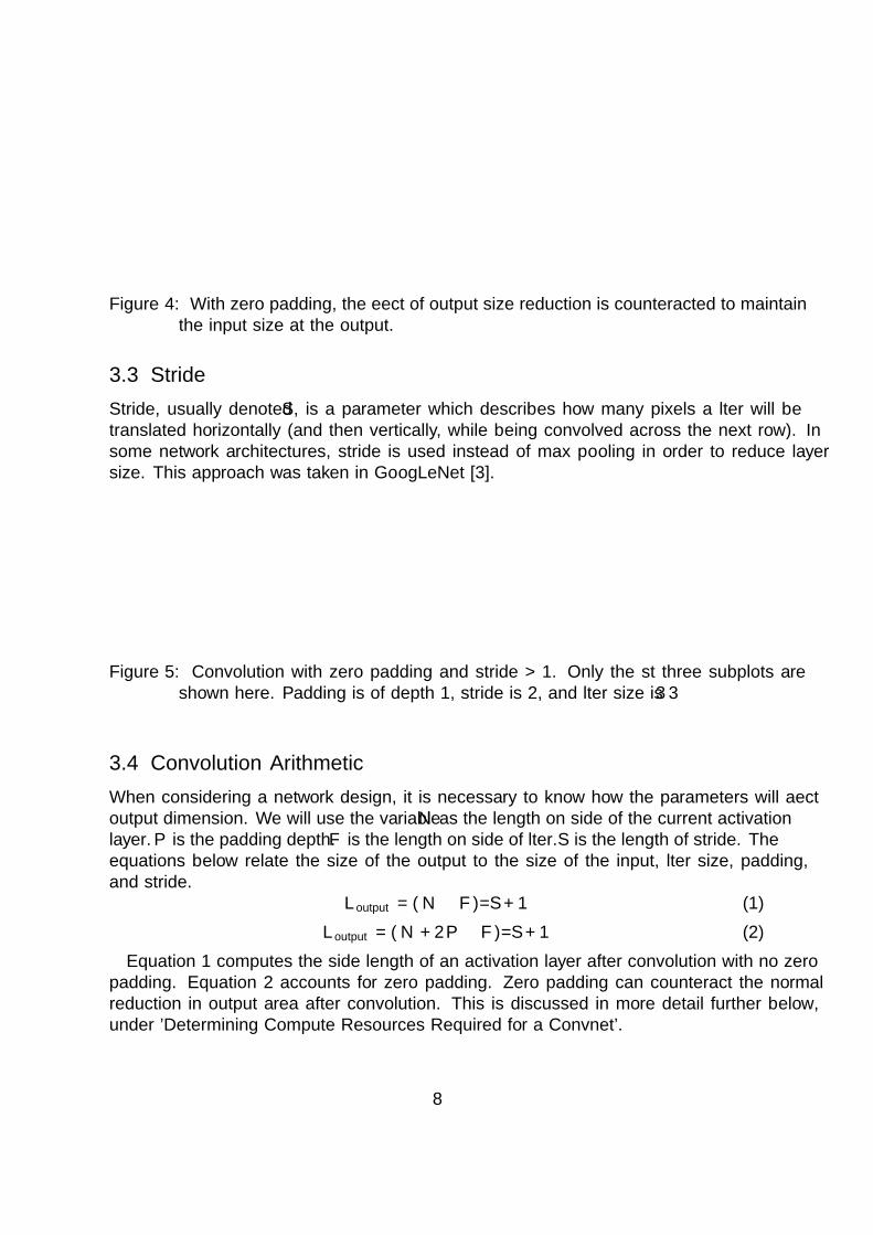
Figure 4: With zero padding, the e�ect of output size reduction is counteracted to maintainthe input size at the output.
3.3 Stride
Stride, usually denoted S, is a parameter which describes how many pixels a �lter will betranslated horizontally (and then vertically, while being convolved across the next row). Insome network architectures, stride is used instead of max pooling in order to reduce layersize. This approach was taken in GoogLeNet [3].
0
0
0
0
0
0
0
0
2
2
3
0
3
0
0
0
0
1
0
3
0
0
0
0
2
1
2
0
0
0
2
2
3
1
0
0
1
2
3
1
0
0
0
0
0
0
0
0
0
0
2
0
1
2
1
2
0
2
6.0
8.0
6.0
4.0
17.0
17.0
4.0
13.0
3.0
0
0
0
0
0
0
0
0
2
2
3
0
3
0
0
0
0
1
0
3
0
0
0
0
2
1
2
0
0
0
2
2
3
1
0
0
1
2
3
1
0
0
0
0
0
0
0
0
0
0
2
0
1
2
1
2
0
2
6.0
8.0
6.0
4.0
17.0
17.0
4.0
13.0
3.0
0
0
0
0
0
0
0
0
2
2
3
0
3
0
0
0
0
1
0
3
0
0
0
0
2
1
2
0
0
0
2
2
3
1
0
0
1
2
3
1
0
0
0
0
0
0
0
0
0
0
2
0
1
2
1
2
0
2
6.0
8.0
6.0
4.0
17.0
17.0
4.0
13.0
3.0
Figure 5: Convolution with zero padding and stride > 1. Only the �st three subplots areshown here. Padding is of depth 1, stride is 2, and �lter size is 3×3
3.4 Convolution Arithmetic
When considering a network design, it is necessary to know how the parameters will a�ectoutput dimension. We will use the variable N as the length on side of the current activationlayer. P is the padding depth. F is the length on side of �lter. S is the length of stride. Theequations below relate the size of the output to the size of the input, �lter size, padding,and stride.
Loutput = (N − F )/S + 1 (1)
Loutput = (N + 2P − F )/S + 1 (2)
Equation 1 computes the side length of an activation layer after convolution with no zeropadding. Equation 2 accounts for zero padding. Zero padding can counteract the normalreduction in output area after convolution. This is discussed in more detail further below,under 'Determining Compute Resources Required for a Convnet'.
8

2
2
3
0
3
0
0
1
0
3
0
0
2
1
2
0
2
2
3
1
1
2
3
1
0
3.0
3.0
3.0
2.0
3.0
3.0
3.0
3.0
3.0
2
2
3
0
3
0
0
1
0
3
0
0
2
1
2
0
2
2
3
1
1
2
3
1
0
3.0
3.0
3.0
2.0
3.0
3.0
3.0
3.0
3.0
2
2
3
0
3
0
0
1
0
3
0
0
2
1
2
0
2
2
3
1
1
2
3
1
0
3.0
3.0
3.0
2.0
3.0
3.0
3.0
3.0
3.0
Figure 6: This is an example of computing the maxpool output at three 3×3 patch locationson an activation layer. Max pooling is applied on 3×3 patches. Max poolingincreases the intensity of pixels upon pooling, since only the maximum intensitypixel was chosen from each pooled area.
For computational reasons, it is best to set the number of �lters to be a power of 2. Thishelps to vectorize computations. Filter sizes are usually odd numbers. This is to have a �ltercenter pixel. This way, the �lter is applied to some position that exists on the input tensor.Note that after convolving a 5×5 pixel image with a 3×3 �lter in Figure 3, the output
(activation layer) has dimensions of 3×3 pixels, which is consistent with Equation 1.
3.5 Pooling
Pooling layers were developed to reduce the number of parameters needed to describe layersdeeper in the network. Pooling also reduces the number of computations required for trainingthe network, or for simply running it forward during a classi�cation task. Pooling layersprovide some limited amount of translational and rotational invariance. However, it will notaccount for large translational or rotational perturbations, such as a face �ipped by 180◦.Perturbations like these could only be detected if images of faces, rotated by 180◦, werepresent in the original training set. Accounting for all possible orientations of an objectwould require more �lters, and therefore more weight parameters would be required.A larger question, however, is whether a simple convnet might be the most appropriate
network architecture for accounting for various representations of the same object class. In2015, Google developed the Inception module which was an architectural module designedfor detecting features with some scale invariance[3]. This is discussed further below. Theinception module is an extension to previous convolutional network architectures. Otherfunctionally distinct network modules have been developed for other purposes, such as re-taining information in a recurring neural network. Examples of this include the Long ShortTerm Memory module (LSTM), and the gated recurring unit (GRU)[10, 11]. It is speculatedhere that more e�ective modules for capturing translational, and rotational invariance maybe developed.Figure 6 shows max pooling applied on 3×3 patches. Because max pooling increases the
intensity of pixels, one might expect that a better way to pool would be to keep the averageintensity per pixel the same. However, this was discovered to not generally be the case.Some convnet architectures, such as GoogLeNet, are replacing max pooling layers by usinglarger strides.
9

4 Network Design Questions
1. How is an adequate number of �lters determined?
2. Given a number of image categories (classes), and the number of images per class,what is the learning capacity of a neural network?
3. How can image classi�cation tasks be expressed in terms of learning capacity require-ments?
More classes imply that more features must be learned. More features require more �lters,and more �lters require more parameters. It would seem that the depth of the networkshould be determined by some measure of complexity common to almost all images in thedata set. Residual networks operate better at arbitrarily large numbers of layers. The relationspeculated here between a su�cient number of layers and a complexity measure of images inthe dataset applies to regular convnets, and not to residual networks. If the number of hiddenlayers required could be determined at the outset, then only the number and size of �ltersfor each layer would be left to determine. The number of classes would primarily determinethe number of �lters. However, because of the e�ectiveness of distributed representation,the number of �lters required will not increase linearly with the number of classes. It mayinstead increase in proportional to some fractional power of it.During training, patches low in the network usually become resolved into edge detectors
[1]. This helps the network to then build more complex representations in the �lters for thenext layer. Also, the small size of �lters used in the �rst layer leaves them little �exibilitybut to pick out only small, nearly featureless structures, such as edges, or blobs of color,for instance. Filters for the next layer then become combinations of �lter features from thecurrent layer.
5 Convnet Training
During network training, the �lter weights are adjusted, so as to improve the classi�cationperformance of the network. This can be done using a method called backpropagation,where the gradient of an error function is computed with respect to all network weights,going all the way to the input connections of the network. Network weights are updated bythe following equation relating the step size to the gradient and the learning rate, denotedη.
Wnew = W − η dEdW
(3)
An error (or "scoring") function can be expressed as a sum of squared di�erences betweenthe network's output and the correct output, over all discrete points in the output. This sortof scoring function works for cases where the network output is a vector, matrix, or tensorof continuous real values.
10

E(W, b) =1
N
N∑i=1
1
2‖hW,b(x
(i))− y(i)‖2 (4)
The gradient of this scoring function would be taken in Equation 3.For classi�cation networks, the scoring function is computed di�erently. Because the
output is a one-of-N vector, where the highest value component represents the network'sbest estimation of the image class (i.e., car, boat, airplane, etc.), an error function forcategorical output is needed. This is called the categorical cross entropy [12], which will notbe explained here, other than to state that it is used to estimate the error in categoricaloutputs, such as with image classi�cation convnets.
5.1 Optimization Methods
Names for optimization methods, both old and new, are listed below.
Stochastic Gradient Descent (SGD)SGD is used with batch processing, where the gradient of a batch is averaged over andused for making network weight updates.
SGD with MomentumWhen momentum is added, jitter in steep gradient directions is reduced, while momen-tum is built in shallow directions.
Nesterov's Accelerated Gradient (NAG)NAG evaluates at the next position indicated by the momentum. This is called a"lookahead" gradient. In practice, NAG almost always converges faster than SGDwith momentum.
AdaGradAdaGrad scales the gradient inversely proportional to the square root of the sum of thesquare of previous gradients. In practice, this means that you can have a larger learningrate than in steep directions. Since the sum of the square of previous gradient willonly grow larger, the learning rate with AdaGrad eventually falls to zero and networklearning stops.
RMSPropRMSProp is similar to AdaGrad, except that a decay parameter is applied to the cachedsum of previous squared gradient values. This has the e�ect of preventing the learningrate from goin to zero, by constantly re-energizing the search.
ADAMADAM combines the concept of momentum with AdaGrad [13].
Stochastic gradient descent derives its name from the random �uctuations of the gradientvector of the scoring function with respect to weights across networks in a batch. Thecomputed gradients are averaged across and the network scoring functions are minimizedusing the average gradient.
11

5.2 Regularization
Regularization is another mechanism for preventing networks from over�tting to the data.A regularization technique called L2 regularization places a penalty on the sum of weightssquared, with a weight decay parameter, denoted λ.
E(W, b) =1
N
N∑i=1
1
2‖hW,b(x
(i))− y(i)‖2 + λ
2
nl−1∑l=1
sl∑i=1
sl+1∑j=1
(W(l)ji )
2 (5)
This sort of regularization results in smaller, more distributed weights, which reduces over�t-ting. Another technique, called L1 regularization, places a penalty on the sum of the absolutevalues of the weights.
E(W, b) =1
N
N∑i=1
1
2‖hW,b(x
(i))− y(i)‖2 + λ
2
nl−1∑l=1
sl∑i=1
sl+1∑j=1
∣∣∣W (l)ji |∣∣∣ (6)
L1 regularization promotes sparsity, and many weights end up being zero.
5.3 Network Weight Initialization
Careful consideration must be given to how a network's weights are initialized. This consid-eration must be made, while keeping in mind the type of non-linear activating function beingused. If weights are initialized too large in magnitude, then a non-linear saturating function,such as tanh, or sigmoid could become saturated in either the positive or negative plateauregions. This is bad because during training by backpropagation it causes the gradient of thenon-linear functions to go to a near-zero value, for those neurons which are in the saturationregion. As more near-zero derivatives are chained on, the gradient becomes essentially zerowith respect to any weight, and network training by backpropagation will not be possible.One method for initializing network weights distributes values randomly, from a Gaussian
distribution, but with the variance inversely proportional to the sum of network inputs andoutputs [14]. A network with more input and output neurons would be initialized withrandom weights drawn from a narrower Gaussian distribution, centered on zero, compared toa network with fewer input and output neurons. This approach was proposed to prevent thebackpropagation gradient from vanishing or exploding. However, in practice, the Ca�e deeplearning framework has implemented a slightly di�erent expression for the variance, whichis inversely proportional to only the number of network inputs[15]. Further research hasdiscovered that, when using ReLU activation units, multiplying the inverse of the number ofinputs by 2 yields a variance which gives the best results [16].
5.4 Dropout
Dropout was a technique developed by [17], for preventing over�tting of a network to theparticular variations of the training set. In fully connected layers, which are prone to over-�tting, dropout can be used, where nodes in a layer will be removed with some de�ned
12
probability, p. Nodes which are removed do not participate in training. After training, theyare replaced in the network with their original weights. This prevents the fully connectedlayers from over�tting to the training data set, and improves performance on the validationset and during deployment.
5.5 Image Data Augmentation
Data augmentation is an e�ective way to increase the size of a data set, while not degradingthe quality of the data set. Training on the augmentation data set yields networks whichperform better than those trained on an unaugmented data set. To augment an imagedata set, the original images can be �ipped horizontally and vertically, and subsamples ofthe original images can be selected at random positions in the original. These subsampledimages can then also be �ipped horizontally and vertically [1].
5.6 Activation Functions
The relation between image class and image data is non-linear. In order for a neural networkto construct the non-linear relation between the data and image class, the activation functionmust have a nonlinearity. Without non-linearities, a neural network would be capable of onlylinear classi�cation.Hyperbolic tangent and sigmoidal activations were used before it was discovered that
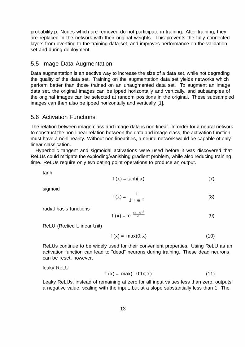
ReLUs could mitigate the exploding/vanishing gradient problem, while also reducing trainingtime. ReLUs require only two �oating point operations to produce an output.
tanhf(x) = tanh(x) (7)
sigmoid
f(x) =1
1 + e−x(8)
radial basis functions
f(x) = e−(x−xi)
2
2α (9)
ReLU (Recti�ed Linear Unit)
f(x) = max(0, x) (10)
ReLUs continue to be widely used for their convenient properties. Using ReLU as anactivation function can lead to "dead" neurons during training. These dead neuronscan be reset, however.
leaky ReLUf(x) = max(−0.1x, x) (11)
Leaky ReLUs, instead of remaining at zero for all input values less than zero, outputsa negative value, scaling with the input, but at a slope substantially less than 1. The
13

resulting piecewise de�ned function looks like the ReLU, but with the zero portionrotated only slightly counterclockwise into Quadrant III. ReLUs can sometimes go"dead" when they get stuck in the zero output plateau region. Leaky ReLUs, on theother hand, do not have this tendency to go "dead" during training.
6 Determining Compute Resources Required for a
Convnet
An example is presented here on how to determine the number of parameters a convnetrequires, and how to determine the number of FLOPs required for a forward or backwardpass through the network. Consider the convnet depicted in Figure 7. The network depicted
Figure 7: A convolutional neural network with max pool layers replaced by convolution layershaving stride 2.
consists of an input layer, an output layer, and �ve hidden layers. Two hidden layers arepatch connected to the previous layer. The last three hidden layers are fully connected tothe previous layer. These are called fully connected, or a�ne layers.If given a 125×125 input image, and sets of 96, 256, 384, and 384 �lters of dimension
5×5 are to be convolved at the �rst, second, third, and fourth convolutional layers, with nozero padding, and with stride 2, then the activation maps will be reduced in dimension, asshown in the table below.
6.1 Parameter Counting
To begin counting the total number of parameters required to describe a network, considerthe network in Figure 7, the �rst convolution is done with 96 �lters. We will use the variableK to represent the number of �lters.
Qparams = K(5× 5× 3 + 1) (12)
The extra 3 arises from the three color channels for the input image.
14

Activation Layer Sizes after Convolution
Convnet LayerActivation LayerSize
input 125×125×3Conv Layer1 61×61×96Conv Layer2 29×29×256Conv Layer3 13×13×384Conv Layer4 5×5×384FC1 1x1x4096FC2 1x1x4096Output 1x1x1000
Table 1: Because of the stride of 2, the activation layers become reduced approximately by afactor of 2 after every convolution. Max pooling is becoming replaced by convnetshaving stride > 1.
The neurons in each successive layer have a bias term adding to the sum over all 25weighted inputs from the �lter. Note that there is only one bias across all three colorchannels. This leads to 126 parameters per �lter: 125 for the weights, and one for the biasterm. In total, the quantity of parameters, Qparams, is then 12,096 (12,000 weights and 96bias terms). The weight parameters then fully describe all 5×5×3+1 parameters for each ofthe 96 �lters.
6.2 Memory Requirement
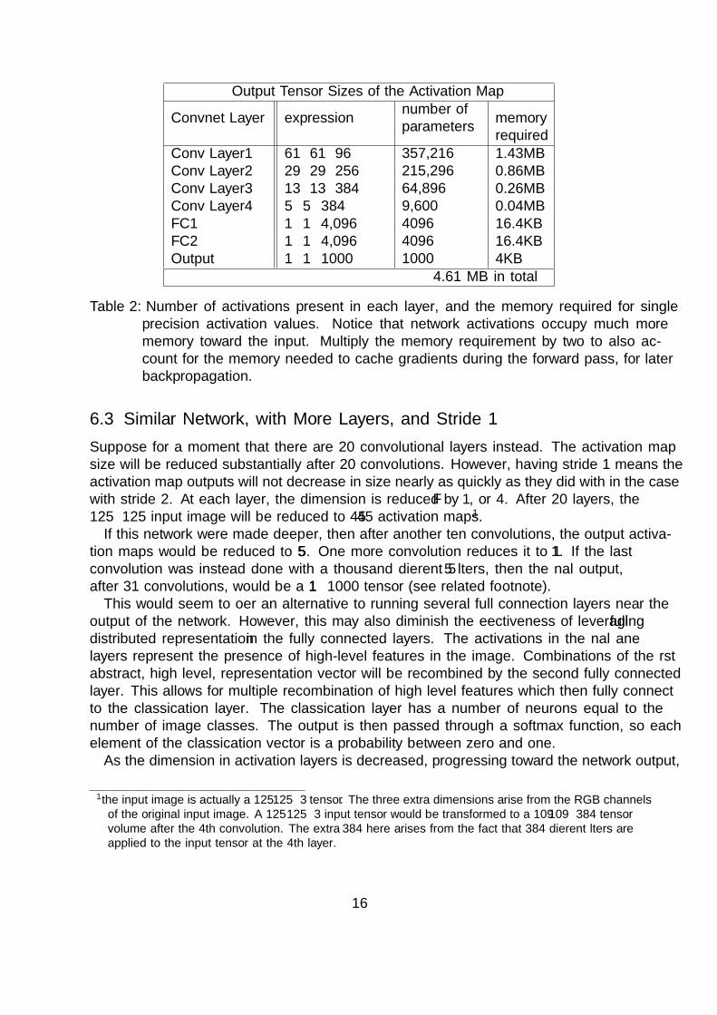
The memory requirement is determined by the memory for the feature map activations. Thememory footprint for a network is twice the total given in Table 2, because the gradients mustalso be stored along the forward pass. As the network is computed forward, the derivativescan be calculated along the way, and both the neurons' activations and gradient of theoutput with respect to neuron weights can be stored in cache. The stored values will thenbe used when backpropagation is computed during training. Some deep learning frameworkswill cache these values during the forward pass.Doubling the memory value in Table 2 yields 9.22MB as the total memory footprint for
one network. On a GPU with 8GB onboard, 867 networks could be �t onto the GPU atonce. However, there is a limit to the batch size, beyond which there is no improvement inthe averaged gradient. A batch size of 256 is common, if the network memory footprint will�t into the GPU memory 256 times.Before we can begin estimating the number of parameters required, we must consider
several parameters related to the �lter itself. These are the stride, �lter size, and zeropadding depth.
15
Output Tensor Sizes of the Activation Map
Convnet Layer expressionnumber ofparameters
memoryrequired
Conv Layer1 61×61×96 357,216 1.43MBConv Layer2 29×29×256 215,296 0.86MBConv Layer3 13×13×384 64,896 0.26MBConv Layer4 5×5×384 9,600 0.04MBFC1 1×1×4,096 4096 16.4KBFC2 1×1×4,096 4096 16.4KBOutput 1×1×1000 1000 4KB
4.61 MB in total
Table 2: Number of activations present in each layer, and the memory required for singleprecision activation values. Notice that network activations occupy much morememory toward the input. Multiply the memory requirement by two to also ac-count for the memory needed to cache gradients during the forward pass, for laterbackpropagation.
6.3 Similar Network, with More Layers, and Stride 1
Suppose for a moment that there are 20 convolutional layers instead. The activation mapsize will be reduced substantially after 20 convolutions. However, having stride 1 means theactivation map outputs will not decrease in size nearly as quickly as they did with in the casewith stride 2. At each layer, the dimension is reduced by F − 1, or 4. After 20 layers, the125×125 input image will be reduced to 45×45 activation maps.1
If this network were made deeper, then after another ten convolutions, the output activa-tion maps would be reduced to 5×5. One more convolution reduces it to 1×1. If the lastconvolution was instead done with a thousand di�erent 5×5 �lters, then the �nal output,after 31 convolutions, would be a 1×1×1000 tensor (see related footnote).This would seem to o�er an alternative to running several full connection layers near the
output of the network. However, this may also diminish the e�ectiveness of leveraging fulldistributed representation in the fully connected layers. The activations in the �nal a�nelayers represent the presence of high-level features in the image. Combinations of the �rstabstract, high level, representation vector will be recombined by the second fully connectedlayer. This allows for multiple recombination of high level features which then fully connectto the classi�cation layer. The classi�cation layer has a number of neurons equal to thenumber of image classes. The output is then passed through a softmax function, so eachelement of the classi�cation vector is a probability between zero and one.As the dimension in activation layers is decreased, progressing toward the network output,
1the input image is actually a 125×125×3 tensor. The three extra dimensions arise from the RGB channels
of the original input image. A 125×125×3 input tensor would be transformed to a 109×109×384 tensor
volume after the 4th convolution. The extra ×384 here arises from the fact that 384 di�erent �lters are
applied to the input tensor at the 4th layer.
16

Network Parameter Count
Convnet Layer expressionnumber ofparameters
memoryrequired
Conv Layer1 (5×5×3+1)×96 12,096 0.05MBConv Layer2 (5×5×96+1)×256 614,656 2.46MBConv Layer3 (5×5×256+1)×256 1,638,656 6.55MBConv Layer4 (5×5×384+1)×4096 39,325,696 157MBFC1 4096×(4096+1) 16,781,312 67.1MBFC2 4096×(4096+1) 16,781,312 67.1MBOutput 4096×(1000+1) 4,100,096 16.4MB
321MB in total
Table 3: Number of parameters required for each network layer, and the memory required forsingle precision parameters. The memory requirements assume that each parameteris 4 bytes, or a single precision �oating point number.
information loss could result, if the number of �lters per layer is not increased at a minimumpace. With a deep network, it is possible to maintain layer size by padding layers beforeconvolving them. An example of this is illustrated in Figure 4. When layer size is maintained,a side e�ect occurs, however, which is that pixels closer to the edge are lower in value, orthey contain redundant information. This e�ect increases in deeper network layers. Evenwith padding, some information loss still occurs.By increasing the number of �lters as the e�ective area of activation layers decreases,
the high dimensional, low-level image information is transformed to low dimensional, high-level information. The central challenge in neural networks is obtaining networks whichperform this transition so that an e�ective, high-level, compressed information representationis produced at the output, e.g., image class.Newer convnet architectures are beginning to replace the fully connected layers in favor
of more convolutional layers. With current trends, better performance is seen when aver-age pooling over an output tensor of activation maps when each cross section is 9×9, orslightly larger. Average pooling here replaces full connections. This approach has been usedwith GoogLeNet, which performed better than previous architectures having fully connectedlayers near the output. This suggests that high level feature recombination in successivefully connected layers is excessive, and that better performance can be obtained with lessrecombination.
6.4 Computational Requirement
Computational requirements for fully connected and convnets are determined di�erently. Thefull connection in multilayer networks allows for the computation to be expressed as a singlematrix multiplication for each layer.Because of the use of �lters, convnets do have have a method as straightforward as a
single matrix computation for determining the number of �oating point operations involved
17
in a single forward pass. New developments have shown that the compute requirement forconvnets can be reduced by using the Strassen algorithm, by a factor down to 1
8[18].
While the number of �oating point operations can be determined, the speed at whichthe total number of operations can be executed depends on the programming language,algorithmic implementation in the application, and the hardware compute capacity, expressedin �oating point operations per second (FLOPS). Host to device communication latenciesalso play a determining factor in program execution speed. Modern GPUs, such as the TeslaP100 have compute capacities of 10.3 TFLOPS for single precision �oating point operations.The use of sigmoidal or tanh activation functions are more expensive than ReLU. ReLU
requires only two FLOPs per output in an activation layer. Sigmoidal and tanh functionsrequire more, since they are represented by a truncated Taylor series expansion.Adding a regularization term to the scoring function, or incorporating dropout into any
layers would complicate determining the computational requirement. This topic will berevisited in another paper.
7 Newer Developments
7.1 Inception Modules
Inception is an architectural element developed to allow for some scale invariance in objectrecognition. If an object in an image is too small, a convnet may not be able to detect itbecause the network �lters were trained to recognize larger versions of the same object. Inother words, a network could be trained to recognize faces very well. But if the face is toofar away in the image, the �lters, trained on larger faces, will not pick out the scaled down,distant face. Inception is able to convolve through the image with various �lter sizes, allat the same computational step in the network. The results are computed and combinedtogether into a single vector.Combining the scale invariance of Inception modules with Residual Networks might result
in an architecture worth investigating [3, 2]. The best features of both GoogLeNet andResNet could possibly be combined into a single network for better performance.As mentioned previously, GoogLeNet does not use fully connected layers at the end of the
network. Instead, it computes average pooling across a 7×7×512 output volume, to yielda 1×1×512 vector. This avoids a substantial portion of the parameters required for fullyconnected layers, and suggests that successive recombination of high level features in fullyconnected layers is excessive for constructing a low dimension, high level representation ofthe image.
7.2 Residual Networks
Microsoft ResNet was the winner of the ILSVRC competition in 2015. Their entry introduceda new architectural design, called residual networks. One of the advantages of residual net-works is that backpropagation does not encounter the vanishing/exploding gradient problem.A network output is determined by the sum of a series of small residual changes made to
18

the original input. Because the gradient can be backpropagated without attenuation withResNets, network architectures can be deeper than anything previously possible. Microsoftintroduced a network having 152 layers (8 times deeper than VGG Net) [2],[19].Previously, increasing network depth past a certain point was shown to actually decrease
network performance. With Residual networks, network performance continues to increasebeyond depths at which regular convnets yielded decreased performance.
8 Conclusion
Several trends have been noted throughout this paper. They are summarized here foroverview.
1. �lters of 3×3 are being used more often, instead of larger �lters, but with more networklayers [19]
2. Fully connected layers are being replaced with average pooling over some output volume
3. With batch normalization, networks can do without dropout and have higher learningrates
Two major architectural improvements have been developed recently. The inception mod-ule, along with residual networks, have improved convnet performance, and introduced newcapabilities. The Inception module provides some scale invariance, while residual networksallow for training deeper networks. Residual networks can train deep networks without thedegradation of performance seen when regular convnets are extended to the number of layersused in Microsoft's ResNet.Several methods for preventing over�tting of a network to training data have been devel-
oped, including:
• convolutional networks with local �lters
• dropout
• data set augmentation
• L2 Regularization
Methods for more e�ective training discussed are:
ReLUUsing ReLU as an activation function speeds up training, and works around the vanish-ing/exploding gradient problem. ReLU can result in "dead" neurons during training.The Leaky ReLU was developed to address this problem.
Xavier Initializationtunes the variance of initial weight distribution to be inversely proportional to thenumber of network inputs
19

ADAM, RMSPropmore recently developed minimization algorithms such as ADAM, and RMSProp resultis faster training times.
Calculating the memory requirement for a convnet will help determine an appropriatebatch size. The exercise illustrated demonstrates how to compute memory requirementsfor a convolutional network with four convolutional layers, and three fully connected layers(including the output layer).
9 Acknowledgements
The code used to generate the �gures illustration discrete convolution is available on GitHub.2.The code used to generate the convolutional neural networks in Figure 2 and Figure 7 is alsoavailable on GitHub.3.
2https://github.com/vdumoulin/conv_arithmetic3https://github.com/gwding/draw_convnet
20
References
[1] Alex Krizhevsky, Ilya Sutskever, and Geo�rey E Hinton. Imagenet classi�cation with deepconvolutional neural networks. In Advances in neural information processing systems,pages 1097�1105, 2012.
[2] Kaiming He, Xiangyu Zhang, Shaoqing Ren, and Jian Sun. Deep residual learning forimage recognition. arXiv preprint arXiv:1512.03385, 2015.
[3] Christian Szegedy, Wei Liue, Yangqing Jia, Pierre Sermanet Sermanet, Scott Reed,Dragomir Anguelov, Dumitru Erhan, Vincent Vanhoucke, and Andrew Rabinovich. Go-ing deeper with convolutions. arXiv preprint arXiv:1409.4842, 2014.
[4] Warren McCulloch and Walter Pitts. A logical calculus of ideas immanent in nervousactivity. Bulletin of Mathematical Biophysics, 5:115�133, 1943.
[5] David Hubel and Torsten Wiesel. Receptive �elds, binocular interaction and functionalarchitecture in the cat's visual cortex. The Journal of physiology, 160:106�154, 1962.
[6] Kunihiko Fukushima. Neocognitron: A self-organizing neural network model for a mech-anism of pattern recognition una�ected by shift in position. Biological Cybernetics,36:193�202, 1980.
[7] Yann Le Cun, Léon Bottou, and Yoshua Bengio. Reading checks with multilayer graphtransformer networks. In Acoustics, Speech, and Signal Processing, 1997. ICASSP-97.,1997 IEEE International Conference on, volume 1, pages 151�154. IEEE, 1997.
[8] Jia Deng, Wei Dong, Richard Socher, Li-Jia Li, Kai Li, and Li Fei-Fei. Imagenet: Alarge-scale hierarchical image database. In Computer Vision and Pattern Recognition.IEEE, 2009.
[9] Matthew D Zeiler and Rob Fergus. Visualizing and understanding convolutional net-works. In Computer vision�ECCV 2014, pages 818�833. Springer, 2014.
[10] Hochreiter, Sepp, and Schmidhuber. Long short-term memory. Neural Computation,9.8:1735�1780, 1997.
[11] Junyoung Chung, Caglar Gulcehre, Kyunghyun Cho, and Yoshua Bengio. Gated feedbackrecurrent neural networks. CoRR, 2015.
[12] Richard Socher, Alex Perelygin, Jean Wu, Jason Chuang, Christopher Manning, AndrewNg, and Christopher Potts. Recursive deep models for semantic compositionality overa sentiment treebank. Proceedings of the conference on empirical methods in naturallanguage processing (EMNLP), 1631, 2013.
[13] Diederik Kingma and Jimmy Ba. Adam: A method for stochastic optimization. arXivpreprint arXiv:1412.6980, 2014.
21

[14] Glorot Xavier and Yoshua Bengio. Understanding the di�culty of training deep feedfor-ward neural networks. Aistats, 9, 2010.
[15] Yangqing Jia, Evan Shelhamer, Je� Donahue, Sergey Karayev, Jonathan Long, RossGirshick, Sergio Guadarrama, and Trevor Darrell. Ca�e: Convolutional architecturefor fast feature embedding. In Proceedings of the ACM International Conference onMultimedia, pages 675�678. ACM, 2014.
[16] Kaiming He, Xiangyu Zhang, Shaoqing Ren Ren, and Jian Sun. Delving deep intorecti�ers: Surpassing human-level performance on imagenet classi�cation. arXiv preprintarXiv:1502.01852, 2015.
[17] Nitish Srivastava, Geo�rey Hinton, and Alex and Krizhevsky. Dropout: A simple wayto prevent neural networks from over�tting. Journal of Machine Learning Research,15:1929�1958, 2014.
[18] Nitish Srivastava, Geo�rey Hinton, Alex Krizhevsky, Ilya Sutskever, and RuslanSalakhutdinov. Dropout: A simple way to prevent neural networks from over�tting.Journal of Machine Learning Research, 15:1929�1958, 2014.
[19] Karen Simonyan and Andrew Zisserman. Very deep convolutional networks for large-scale image recognition. arXiv preprint arXiv:1409.1556, 2014.
22