exploring ligand affinities for proteins by nmr of long ... spin-pair labeling for ligand lls ......
TRANSCRIPT

POUR L'OBTENTION DU GRADE DE DOCTEUR ÈS SCIENCES
acceptée sur proposition du jury:
Prof. D. L. Emsley, président du juryProf. G. Bodenhausen, Dr C. Dalvit, directeurs de thèse
Dr W. Jahnke, rapporteurDr E. Chiarparin, rapporteuseProf. K. Johnsson, rapporteur
Exploring Ligand Affinities for Proteins by NMR of Long-Lived States
THÈSE NO 6816 (2015)
ÉCOLE POLYTECHNIQUE FÉDÉRALE DE LAUSANNE
PRÉSENTÉE LE 11 DÉCEMBRE 2015
À LA FACULTÉ DES SCIENCES DE BASELABORATOIRE DE RÉSONANCE MAGNÉTIQUE BIOMOLÉCULAIRE
PROGRAMME DOCTORAL EN CHIMIE ET GÉNIE CHIMIQUE
Suisse2015
PAR
Roberto BURATTO


“Twenty years from now you will be more
disappointed by the things that you didn’t
do than by the ones you did do. So throw
off the bowlines. Sail away from the safe
harbor. Catch the trade winds in your sails.
Explore. Dream. Discover.”
Mark Twain


Abstract
i
Abstract
The detection of molecules that can bind to active sites of protein targets and the
measurement of their affinities is a promising application of NMR. Nowadays, the
screening of drug candidates is routinely done by NMR in pharmaceutical industry.
We have proposed to use the relaxation of Long-Lived States (LLS) for drug screening by
NMR. Long-lived states are nuclear spin states whose decay time constant 𝑇𝐿𝐿𝑆 can be
much longer than the longitudinal relaxation time 𝑇1. LLS can be used to screen and
determine the dissociation constant 𝐾𝐷 of molecular fragments that bind weakly to protein
targets. The use of LLS for fragment screening leads to a spectacular increase in contrast
between free and bound ligands, and thus allows one to characterize binding of fragments
with very weak affinities, with 𝐾𝐷 in the millimolar range, which is difficult to achieve by
other methods such as ITC. By exploiting the LLS behavior of a spy molecule, we
experimentally demonstrate that it is possible to measure dissociation constants KD as
large as 12 mM, corresponding to very weak binding, where most other biophysical
techniques fail, including other NMR methods based on the observation of ligands.
Furthermore, we have combined LLS for screening for improved contrast with 1H
dissolution-DNP to enhance the sensitivity. DNP-enhanced screening for measuring LLS
signals of a weak ligand allows one to use very low concentrations of ligands and proteins.
We observed dramatic differences between the spectra of the ligand in the presence or
absence of a protein, or in the presence of the protein combined with a stronger ligand.
Moreover, we have explored LLS involving pairs of 19F nuclei to study binding phenomena.
Indeed, fluorine detection is quite interesting because it offers the possibility to perform
screening experiments without any problems due to overlapping signals. In a custom-
designed fluorinated ligand that binds trypsin, we have observed a promising ratio 𝑇𝐿𝐿𝑆 /
𝑇1 > 4. This fluorinated ligand has been used as spy molecule in competition experiments,
which allowed us to rank the affinities and estimate dissociation constants of arbitrary
ligands that do not contain any fluorine.
Keywords: drug discovery, fragment screening, ligand binding, competition experiments,
Long-Lived States, dynamic nuclear polarization, trypsin, Hsp90, fluorine.

ii

Sommario
iii
Sommario
La rilevazione di molecole che si legano al sito attivo di proteine e la misura della loro
affinità è una promettente applicazione dell’NMR. Nell’industria farmaceutica, al giorno
d’oggi lo screening di molecole con potenziale farmaceutico è abitualmente eseguito con
tecniche NMR.
Abbiamo proposto l’uso del rilassamento degli stati a lunga vita (LLS) per lo screening di
ligandi tramite NMR. Gli stati a lunga vita sono stati di spin nucleari la cui costante di
rilassamento 𝑇𝐿𝐿𝑆 può essere molto più lunga della costante di rilassamento longitudinale
𝑇1. Gli LLS possono essere utilizzati per selezionare ligandi e determinare la costante di
dissociazione 𝐾𝐷 di frammenti molecolari che si legano debolmente a proteine. L’uso degli
LLS per lo screening di frammenti molecolari permette uno spettacolare aumento del
contrasto tra ligandi liberi e legati, permettendo quindi di caratterizzare il legame di
frammenti con affinità molto deboli, con 𝐾𝐷 nell’ordine del millimolare. Questo è un
traguardo normalmente molto difficile da raggiungere con altri metodi, per esempio con
l’ITC. Sfruttando il comportamento degli LLS in una molecola spia, abbiamo dimostrato
sperimentalmente che è possibile misurare costanti KD fino a 12 mM, corrispondenti a
legami molto deboli, dove molte altre tecniche biofisiche falliscono, compresi molti metodi
NMR basati sull’osservazione dei ligandi.
Inoltre, abbiamo combinato l’alto contrasto dello screening effettuato tramite LLS con la
DNP per aumentare la sensibilità dell’esperimento NMR. L’uso della DNP per misurare i
segnali LLS di un ligando debole permette l’uso di concentrazioni molto basse di ligando
e proteina. Con questo approccio, abbiamo osservato enormi differenze tra gli spettri del
ligando in presenza o in assenza della proteina, o in presenza della proteina e di un
ligando più forte.
In aggiunta, abbiamo testato la possibilità di usare LLS su coppie di nuclei di fluoro per
studiare questo tipo di fenomeni. Infatti, la rilevazione dei segnali del fluoro è piuttosto
interessante perchè offre la possibilità di eseguire esperiementi di screening evitando
problemi derivanti dalla sovrapposizione di segnali. In un ligando fluorurato che si lega
alla tripsina, abbiamo misurato un promettente rapporto 𝑇𝐿𝐿𝑆 / 𝑇1 > 4. Questo ligando
fluorurato è stato usato come molecola spia in esperimenti di competizione,
permettendoci di confrontare le affinità e stimare le costanti di dissociazione di ligandi che
non contengono atomi di fluoro.

Sommario
iv
Keywords: drug discovery, screening di frammenti, esperimenti di competizione, stati a
lunga vita, polarizzazione dinamica nucleare, tripsina, Hsp90, fluoro.

Contents
v
Table of Contents
Abstract ............................................................................................................................ i
Sommario ....................................................................................................................... iii
1. Introduction ................................................................................................................ 1
1.1 The drug discovery and development process ....................................................... 2
1.1.1 The drug discovery phase ................................................................................ 3
1.1.2 The drug development phase .......................................................................... 4
1.2 Fragment-Based Drug Discovery ........................................................................... 6
1.2.1 What is a fragment? ......................................................................................... 9
1.2.2 Ligand efficiency ............................................................................................ 10
1.2.3 FBDD compounds in clinical trials .................................................................. 10
1.2.4 Screening of fragments libraries .................................................................... 12
1.2.4.1 Biochemical assays at high concentration ............................................. 13
1.2.4.2 Biophysical techniques ........................................................................... 13
References .............................................................................................................. 19
2. Nuclear magnetic resonance for ligand screening ............................................... 23
2.1 The dissociation constant ..................................................................................... 24
2.1.1 Dissociation constants in competitive binding equilibria ................................. 26
2.2 Effect of binding on NMR parameters ................................................................... 28
2.3 Ligand-based and receptor-based screening ....................................................... 30
2.4 Receptor-based methods ...................................................................................... 31
2.5 Ligand-based methods ......................................................................................... 32
2.5.1 Transverse relaxation rates ............................................................................ 34
2.5.2 Paramagnetic relaxation enhancement .......................................................... 36
2.5.3 Longitudinal relaxation rates .......................................................................... 37

vi
2.5.4 Transverse 19F relaxation ............................................................................... 39
2.5.5 Translational diffusion .................................................................................... 42
2.5.6 Transferred NOEs .......................................................................................... 43
2.5.7 NOE pumping ................................................................................................ 44
2.5.8 Saturation transfer difference ......................................................................... 45
2.5.9 WaterLOGSY ................................................................................................. 47
References ................................................................................................................. 50
3. Nuclear Long-Lived States ..................................................................................... 55
3.1 The principle of symmetry-switching ..................................................................... 57
3.2 Applications .......................................................................................................... 59
3.3 Long-Lived States: the principles ......................................................................... 60
3.4 The singlet NMR experiment ................................................................................ 64
3.4.1 TSI preparation .............................................................................................. 65
3.4.2 TSI storage .................................................................................................... 66
3.4.3 Detection ......................................................................................................... 68
3.4.4 LLS pulse sequence ....................................................................................... 69
3.5 Relaxation of Long-Lived States ........................................................................... 73
3.5.1 The homogeneous master equation .............................................................. 76
3.5.2 The dipolar relaxation mechanism ................................................................. 77
References ................................................................................................................. 79
4. The use of Long-Lived States for studying ligand-protein interactions ............. 83
4.1 LLS contrast ......................................................................................................... 84
4.2 Competition experiments ...................................................................................... 88
4.3 Spin-pair labeling for ligand LLS experiments ...................................................... 91
4.4 Hyperpolarized LLS ligand screening experiments .............................................. 95
4.5 Exploring weak ligand-protein interactions by LLS ............................................... 99
4.6 Extending LLS ligand screening to 19F nuclei ..................................................... 104
References ............................................................................................................... 109

Contents
vii
5. Experimental procedures ...................................................................................... 115
5.1 Ligand titrations .................................................................................................. 115
5.2 Fitting of titration curves ..................................................................................... 115
5.3 Hyperpolarized LLS experiments ....................................................................... 116
5.4 Chemical synthesis of ligands ............................................................................ 116
References ............................................................................................................... 119
6. Conclusions ........................................................................................................... 121
Acknowledgements ..................................................................................................... 125
Curriculum Vitae .......................................................................................................... 129

viii

Chapter 1. Introduction
1
1. Introduction
he overall cost of the development of a new drug is about $800 million to $1
billion.[1] These numbers may seem to be exaggerated, but two factors can
explain them. The first one is the complexity of the research and development
process: for every 5000-10000 compounds that enter the selection process, on average
only one gets approved for the market. Hundreds of other molecules are dropped during
the intermediate selection steps and the final cost must include the expense of these
failures. The second reason is the length of the process: on average 10-15 years are
needed to develop a new drug from the beginning of the discovery campaign to the final
approval. These numbers are quite impressive. It means that a drug which enters into the
market today is the result of a process that has started in the 2000. At that time, the twin
towers were still standing and Wikipedia did not yet exist.
T

1.1 The drug discovery and development process
2
1.1 The drug discovery and development process
uring the past 40 years there has been a huge acceleration in the understanding
of molecular mechanisms that underlay disease processes. As a consequence,
modern pharmaceutical research has become progressively based on target-
focused discovery, where the aim is to modulate the biological activity of a particular
molecular target and thus provide a cure for a disease. The ‘post-genome era’ has further
increased the number of targets of therapeutic interest for which there are not yet known
small-molecule modulators, stimulating many new studies and opening the way to fight
diseases that were hitherto incurable.
The entire process consists in two parts. The first one is the phase of “drug discovery”,
during which a few molecules are identified, studied and optimized in order to be
subsequently tested as potential drugs. The second one is called “drug development”
and consists of an ensemble of clinical tests needed to get the final approval for marketing.
Figure 1 The drug discovery and development timetable. After the target identification, screening campaigns are performed in order to identify a few hit compounds, which have to be optimized in order to address requirements such as affinity, specificity, absorption, distribution, metabolism, excretion and toxicological properties (ADMET). Before accessing to the clinical trials, the compounds have to pass some preclinical tests, in order to verify their efficacy and safety. During the clinical trials, composed of three phases, potential drugs are tested on humans in order to test the safety and efficacy and to optimize the dose. At the end of these clinical phases, the FDA decides if the molecule can go to the market. The whole process can take 10-15 years.
D

Chapter 1. Introduction
3
1.1.1 The drug discovery phase
The first step of drug discovery is the understanding of a disease. Scientists try to
understand how genes are altered, how proteins are overexpressed, etc., and how these
abnormalities affect the health of the patients. In many cases, the major
biopharmaceutical companies are not the only sources of knowledge of this step; many
smaller companies, research centers, universities and other nonprofit institutions provide
significant contributions to the basic knowledge of the disease etiology.
Once the knowledge of a disease allows it, pharmaceutical researchers select a target for
a potential new drug. Already at this step there is the risk of failure: the chosen target has
to be “druggable”, i.e., it should be possible to regulate its activity with high affinity and
selectivity by a drug-like molecule, and its role in the disease has to be validated. In other
words, researchers have to demonstrate that the chosen target is relevant to the disease
being studied through experiments in both living cells and in animal models of the disease.
A recent study estimated that among the 30000 genes in the human genome, only 3000
might code for druggable proteins.[2] Only about 400 of such targets have been studied
so far.
Once the target is chosen, scientists look for a molecule, a “hit compound”, which may act
on it to alter the course of the disease. There are different approaches to search for a hit
compound:
- Natural compounds: molecules present in nature can be starting points for
developing a new drug;
- De novo: computer modeling can be used to design a molecule from structure base
knowledge that may bind and modulate the target’s activity;
- Screening: Few hundred thousand up to few millions compounds can be tested
against the target to identify promising compounds;
- Biotechnology: Researchers can genetically engineer living systems to produce
biological molecules that can fight a disease.
The next phase involves its optimization. The aim is to enhance properties such as
specificity, efficiency and safety. Typically scientists synthetize hundreds of analogues of
the initial hit and test them with the aim of improving the above-cited properties. For
example, they can make the compound less likely to interact with other chemical pathways
in the body, thus reducing potential side effects. The resulting molecule is called lead
compound.

1.1.1 The drug discovery phase
4
Once a few lead compounds have been identified, they have to go through a series of
tests to study their pharmacokinetics properties. In fact, a drug should be 1) absorbed into
the bloodstream, 2) distributed to the proper site of action, 3) metabolized efficiently and
effectively, 4) successfully excreted from the body and 5) demonstrated not to be toxic.
Before being allowed to test a candidate drug on humans, several preclinical tests need
to be performed. Scientists have to understand how the drug works and what its safety
profile looks like. Several in vitro and in vivo tests need to be carried out. Agencies like
the FDA (Food and Drug Administration) require the molecules to go through severe tests
before being applied to humans.
All the above steps can take from three to six years. After starting with 5000-10000
molecules, scientists may have identified a group reduced to one to five molecules which
will be studied in clinical trials as candidate drugs.
1.1.2 The drug development phase
Before starting any clinical trials, an Investigational New Drug (IND) application has to be
submitted to the FDA. This file includes the results of the preclinical work, the molecular
structure and the hypothetical mechanism of action in the body, a list of any side effects
and a detailed clinical plan for the next studies. FDA must be regularly updated on results
of on-going tests and can stop the trials at any time if problems arise.
In Phase 1 trials, the candidate drug is tested on about twenty to one hundred healthy
volunteers. These are the first tests on humans and they are mainly aimed at getting
information on the safety profile and the definition of the safe dosing range.
In Phase 2 trials the potential drug is tested on about 100 to 500 patients who suffer from
the disease. The aim of these tests is to evaluate the effectiveness of the drug, while
keeping possible short-time side effects under observation. In this stage, scientists also
optimize the dose strength and schedules for use of the drug.
In Phase 3 trials, the candidate drug is tested on a larger number (about 1000-5000)
patients to get statistically significant data about safety, efficacy and overall benefit-risk
relationship of the drug. This is the costliest, longest and most critical phase.
At the end of the third phase, all data are evaluated. If the results demonstrate that the
potential drug is safe and effective, the company can file a New Drug Application (NDA)
to the FDA requesting approval to market the drug. At this point, FDA reviews the
application and can decide to 1) approve the medicine, 2) request more information or
studies, or 3) deny approval.

Chapter 1. Introduction
5
It can take 7-9 years from the first tests of Phase 1 and the FDA approval. Research on a
new drug continues even after approval since potential long-term side effects can occur.
The company is asked to submit periodic reports to the FDA.
A famous proverb says “Rome wasn’t built in a day”. “Neither was a drug generated in a
day”, we could add.

1.2 Fragment-Based Drug Discovery
6
1.2 Fragment-Based Drug Discovery
owadays, the search for hit compounds is usually achieved through screening
campaigns. Large libraries (>105) of molecules are usually screened against the
target of interest and their potential interactions are detected by biochemical or
cell-based functional assays. The molecules identified through this procedure, called
High-Throughput Screening (HTS), are then optimized via medicinal chemistry in order to
improve their pharmacokinetic properties.
Progress in robotics and engineering allows one to accelerate the speed of the process.
Nowadays, it is possible to monitor up to 100 million reactions in ten hours.[3]
Nevertheless, the use of HTS has often proven to be inefficient for drug discovery resulting
often in false positive and false negatives. About half of the HTS campaigns fail, mainly
because the library does not contain any good small molecules as starting points.[4] The
probability to fail is even higher for new classes of targets, such as protein-protein
interactions (PPIs), for which there are not many historical precedents.[5, 6]
The hit molecules identified through this strategy may be complex and suffer from a
substantial lipophilicity. These compounds therefore often have limitations with respect to
the criteria of Absorption, Distribution, Metabolism, Excretion and Toxicological (ADMET)
that cannot be easily overcome during the following optimization step.
Table 1 Main differences between Fragment-Based Drug Discovery (FBDD) and High-Throughput
Screening (HTS)
N
FBDD
HTS
About 103 compounds of small size (<300 Da) >105 compounds (>300 Da)
High coverage of chemical space Poor coverage of chemical space
Low-affinity hits (100 µM < KD < 10 mM)
High-affinity hits (KD in the low µM or
stronger)

Chapter 1. Introduction
7
In the past decade, an alternative approach called Fragment-Based Drug Discovery
(FBDD) has emerged. FBDD involves the use of small libraries of fragments that are low
molecular weight compounds. The idea is that scientists can look for small binding
fragments and then either expand a fragment or combine two of them to achieve the
affinity one expects from HTS.
The top part of Figure 2 shows an example of high-throughput screening: many
compounds are screened against a target to identify a hit that binds. This will be then
optimized through medicinal chemistry. The central part of Figure 2 represents the
fragment-linking approach: the screening identifies two small molecules that bind to
nearby sites. They can then be linked together and optimized via medicinal chemistry.
This is the principle of a well-known strategy known as structure-activity relationship
(SAR), implemented by NMR for the first time by Fesik and co-workers.[7]
Figure 2 Graphical representation of the main approaches to develop a drug. (Top) In high throughput screening (HTS), libraries of relatively complex molecules are screened to identify hit compounds with high potency. (Middle) in FBDD, screening can identify fragments that can be successively merged in order to generate a ligand with higher potency. (Bottom) in FBDD, a fragment with low affinity can be identified and then optimized to improve its potency via medicinal chemistry.

1.2 Fragment-Based Drug Discovery
8
Although extremely elegant, many scientists have found that the linking is much more
challenging than might be expected. The main difficulty is that much of the potency of the
two fragments will be lost if they are not perfectly positioned, so that the affinity of the
resulting molecule will not be as good as expected. Therefore, a frequently used
alternative strategy is “fragment growing”, shown in the bottom part of figure 2: a single
fragment is expanded or “grown” by medicinal chemistry to increase the potency of the
initial fragment.
The hit rates of screening campaigns of fragment libraries is usually higher than those of
HTS. This is due to the fact that the larger the molecules, the more complex their
structures. As consequence, each additional moiety has an increasing probability of
interfering with binding. On the other hand, fragments give an opportunity to better sample
the active site of the target, giving important information to medicinal chemists, who have
to link different fragments or to optimize one of them.
Figure 3 Correlation between the potency and the molecular mass of molecules considered in FBDD and HTS, and of approved drugs. Reproduced from [8]. FBDD starts with smaller and less potent molecules, giving medicinal chemists more opportunities to improve important properties needed to develop a successful drug.
Chapter 1. Introduction
9
1.2.1 What is a fragment?
The idea of FBDD to work with small fragments has been supported by some empirical
evidence, summarized in Lipinski’s famous rule of five (RO5).[9] Lipinski and co-workers
observed that most orally administered drugs are relatively small and moderately lipophilic
molecules. Note that the rule of five does not apply to certain classes of drugs, for example
to antiviral drugs.
Based on these observations, the rule summarizes molecular properties which turn out to
be important for the pharmacokinetics of a drug:
1) The molecular mass should be less than 500 Da. This allows one to work with
molecules that can efficiently explore the binding pocket and represent the variety
of chemical space;
2) An octanol-water partition coefficient log P (ClogP) not greater than 5. Solubility is
a critical parameter for fragment libraries. Fragments require a certain level of
hydrophilicity to be soluble up to 1-2 mM, but they should be sufficiently
hydrophobic to interact properly with the target; indeed, many of the druggable
protein targets have pockets with strong hydrophobic contributions to binding;
3) No more than 5 hydrogen bond donors;
4) No more than 10 hydrogen bond acceptors;
Lipinski’s rules have been successively refined for the fragments. Results of the analysis
of a diverse set of fragment hits show that such hits seem to obey a ‘rule of three’
(RO3).[10] The average molecular weight is less than 300 Da, the number of hydrogen
bond donors is not greater than 3, the ClogP is less than 3, and the number of hydrogen
bond acceptors is not greater than 3. In addition, the results suggest that the number of
rotatable bonds (NROT) should not be greater than 3 and the polar surface area (PSA)
should not be greater than 60 Å2.
These are only guidelines, but nowadays many companies follow them while designing
libraries of fragments.

1.2.2 Ligand efficiency
10
1.2.2 Ligand efficiency
We could assume that a fragment behaves like an ant. If it invades a picnic, a guy can
easily squash it. But if he watches the ant escape with a crumb, the answer is different:
ants can carry at least ten times their own body weight.
It is the same for fragments. Due to their small size, fragments bind their target very
weakly. Despite of this, they often bind tightly for their dimensions. In order to express the
binding affinity of a fragment in the light of its molecular mass, the most widely used
parameter is called ligand efficiency (LE).[11] LE can be defined as the ratio between the
free energy of ligand binding and the number of heavy atoms in the ligand. The ‘free
energy of ligand binding’, Δ𝐺𝑏𝑖𝑛𝑑, is equal to -RTln𝐾𝐷, where R is the ideal gas constant,
T the temperature, and 𝐾𝐷 the dissociation constant. The number of heavy atoms refers
to the number of non-hydrogen atoms in the ligand. Alternative parameters exist, as the
binding efficiency index (BEI), which is defined simply as the ratio between the free energy
of ligand binding and the molecular weight.
A drug with a 𝐾𝐷 of 10 nM and a molecular weight of 500 Da (about 38 heavy atoms)
would have LE = 0.3 Kcal/mol/heavy atom. Thus, the aim is to reach ligand efficiencies of
0.3 Kcal/mol/heavy atom or better. Ligand efficiency values can vary considerably based
on the target: for many kinases, inhibitors can have LE above 0.5 Kcal/mol/heavy atom,
while for more challenging targets (as most protein-protein interactions) LE can fall below
0.3 Kcal/mol/heavy atom.
1.2.3 FBDD compounds in clinical trials
Table 2 shows an updated list (January 2015) of drugs that entered clinical trials starting
from fragments. Almost half of the targets are protein kinases, demonstrating that it is
relatively straightforward to identify fragments with high LE that bind to the purine-binding
site of this class of proteins.
August 17th, 2011, marked history of FBDD, when the FDA approved the first drug deriving
from fragment-based screening. The drug is sold with the name Zelboraf (vemurafenib)
and targets a mutant of kinase B-Raf. It can extend life of patients with metastatic
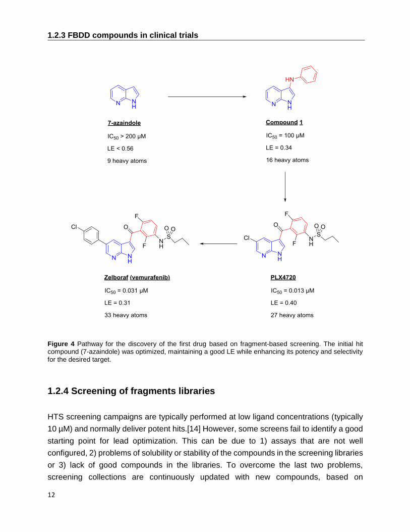
melanoma, where it displayed an impressive activity.[2, 12] Vemurafenib was discovered
at Plexxikon and developed in partnership with Roche. It is the result of a particularly rapid

Chapter 1. Introduction
11
drug discovery and development process: initiated in February 2005, it took just six years
to reach approval. Figure 4 shows the initial fragment and its optimization into the final
drug, reporting the potency and ligand efficiency of each step.
Drug candidate Company Role
Approved Vemurafenib Plexxikon B-Raf(V600E) inhibitor
Phase 2/3
ABT-199 Abbott selective Bcl-2 inhibitor
LEE011 Novartis/Astex CDK4 inhibitor
MK-8931 Merck BACE1 inhibitor
Phase 2
AT13387 Astex HSP90 inhibitor
AT7519 Astex CDK1,2,4,5 inhibitor
AT9283 Astex Aurora, Janus kinase 2 inhibitor
AUY922 Vernalis/Novartis HSP90 inhibitor
Indeglitazar Plexxikon pan-PPAR agonist
Linifanib (ABT 869) Abbott VEGF & PDGFR inhibitor
LY2886721 Lilly BACE1 inhibitor
LY517717 Lilly/Protherics FXa inhibitor
Navitoclax (ABT 263) Abbott Bcl-2/Bcl-xL inhibitor
AZD5363 AstraZeneca/Astex/CR-UK AKT inhibitor
AZD3293 AstraZeneca/Astex/Lilly BACE1 inhibitor
PLX3397 Plexxikon FMS, KIT, and FLT-3-ITD inhibitor
Phase 1
ABT-518 Abbott MMP-2 & 9 inhibitor
ABT-737 Abbott Bcl-2/Bcl-xL inhibitor
AZD3839 AstraZeneca BACE1 inhibitor
DG-051 deCODE LTA4H inhibitor
IC-776 Lilly/ICOS LFA-1 inhibitor
JNJ-42756493 J&J/Astex FGFr inhibitor
AT13148 Astex AKT, p70S6K inhibitor
LP-261 Locus Tubulin binder
LY2811376 Lilly BACE1 inhibitor
PLX5568 Plexxikon kinase inhibitor
SGX-393 SGX Bcr-Abl inhibitor
SGX-523 SGX Met inhibitor
SNS-314 Sunesis Aurora inhibitor
AZD5099 AstraZeneca Bacterial topoisomerase II inhibitor
RG-7129 Roche BACE1 inhibitor
Undisclosed Vernalis/Servier Bcl-2 inhibitor
Table 2 Drug candidates currently under clinical evaluation (January 2015).[13]
1.2.3 FBDD compounds in clinical trials
12
Figure 4 Pathway for the discovery of the first drug based on fragment-based screening. The initial hit compound (7-azaindole) was optimized, maintaining a good LE while enhancing its potency and selectivity for the desired target.
1.2.4 Screening of fragments libraries
HTS screening campaigns are typically performed at low ligand concentrations (typically
10 µM) and normally deliver potent hits.[14] However, some screens fail to identify a good
starting point for lead optimization. This can be due to 1) assays that are not well
configured, 2) problems of solubility or stability of the compounds in the screening libraries
or 3) lack of good compounds in the libraries. To overcome the last two problems,
screening collections are continuously updated with new compounds, based on
Chapter 1. Introduction
13
experience that has been gathered during other screening campaigns, in view of
achieving a better coverage of chemical space.
Another approach is to screen libraries of fragments, which due to their size and low
complexity are likely to interact much more weakly with the target. This therefore requires
one to reconfigure screening assays for much higher concentrations. Issues of solubility
of screening compounds are aggravated by the high concentrations used. Small quantities
of organic solvents like DMSO can be used to improve the solubility and light scattering
techniques can be employed to confirm the absence of aggregates.[12]
There are two ways to carry out fragment screening: biochemical screening (High
Concentration Screening, HCS) or biophysical screening.
1.2.4.1 Biochemical assays at high concentration
This approach consists in performing classical biochemical assays, but working at higher
concentrations (up to 1 mM). In this way, it is possible to use the same technology used
for the classical high-throughput screening technology for detection, and one can identify
some hits very quickly. In addition, the amounts of protein required are very small and
many ‘difficult’ targets (like GPCR or ion channel targets) can be studied. Nevertheless,
many problems can occur. For example, high ligand concentrations can interfere with the
assay or be toxic for cells. Moreover, compound aggregations can give rise to false
positives, or false negatives can result from a lack of solubility of the compounds.
1.2.4.2 Biophysical techniques
There are several biophysical techniques to screen fragments. Different biophysical
techniques have different problems and provide complementary information about
binding. For example, quantitative affinity data can be obtained from isothermal titration
calorimetry (ITC), surface plasmon resonance (SPR), or NMR spectroscopy, while X-ray
crystallography can provide detailed atomic resolution of the binding mode.
Throughput and material requirements can differ dramatically between different
techniques, determining the stage of the FBDD campaign for which they are best suited.
Primary screening is carried out using techniques with high throughput that require small
amounts of target protein, while secondary screening can be performed with techniques
that have a lower throughput. Traditionally, X-ray crystallography and ITC are considered

1.2.4.2 Biophysical techniques
14
as low throughput techniques, while SPR and thermal shift measurements are higher
throughput methods. Depending on whether ligand- or target-detected techniques are
used, NMR spectroscopy can offer a high or low throughput and potentially provide an
atomic model of binding.
X-ray crystallography
X-ray crystallography provides direct information about the binding mode at atomic
resolution.[15] Usually, protein crystals are soaked with a solution containing high
concentrations (about 50 mM) of the fragment and binding is detected directly by
observation of the fragment bound to the protein in the electron density. There is no risk
of false positives, but false negatives can occur when binding sites are occluded by crystal
contacts or when ligand binding requires a conformational change of the target protein
that is inhibited by the crystal framework. The latter problem can be avoided by attempting
co-crystallisation of the protein in the presence of the ligand. In general, X-ray
crystallography provides high resolution data, and is able to detect fairly weak binders, up
to KD ~ 5 mM .
The low throughput of the technique does not allow its use for primary screening, but it is
generally considered as the gold standard for final hit validation. Furthermore, the
throughput of X-ray crystallography has recently been increased.[16] The use of
automated, rapid data collection at powerful synchrotron beam sources that allow the
collection of high-resolution data in minutes, employing sample-changing robots, and
semi-automatic processing and structure solution has speeded up the process
considerably. Molecular replacement strategies can reduce structure solution to manual
inspection of ligand placements in different electron maps. Ligand orientations are
obtained by ligand fitting routines, employing similar strategies as those used in molecular
docking [17], with the advantage to optimize the fit of the ligand with the experimental
electron density. If a cocktail of several ligands is used, it is important to use a diverse set
of ligands to make them identifiable from the shape of their electron density, and to
minimize the chances that two or more ligands compete for the same binding site.
The technique requires the protein of interest to crystallize in a reproducible way.
Problems of solubility of the ligand can be addressed by using low concentrations of
organic co-solvents, such as 1 to 10% DMSO. X-ray crystallography does not provide
information about binding affinities, so X-ray observations must be combined with data

Chapter 1. Introduction
15
obtained by other methods. Ideally, X-ray crystallography should be used in conjunction
with a method with higher throughput like SPR, or verified by ITC after crystallization.
NMR spectroscopy
NMR spectroscopy was the first technique used for experimental FBDD screening.[18] In
the SAR by NMR methodology [7], the binding of a fragment to a protein is detected
through the change in protein chemical shifts. These changes are due to the different
chemical environments experienced by the nuclei of the protein upon binding. In its first
application, two fragments identified in this way were merged, yielding a binder with
improved potency.[16]
SAR by NMR is an example of target-detected method. In such methods, the chemical
shifts of the target protein are observed in two-dimensional NMR experiments. As a
consequence, these methods are limited to small proteins with molecular masses of about
30 to 40 kDa and require relatively large amounts of isotope-labelled proteins. On the
other side, target-detected methods can provide information about the binding site, if the
protein resonance assignments are available.
As an alternative, several ligand-detected methods have been developed, such as
Saturation Transfer Difference (STD) [19], WaterLOGSY [20] or Target-Immobilized NMR
Screening (TINS).[21] These methods require less protein, no isotope labelling, and are
also applicable to larger proteins. On the other hand, they usually do not provide
information about the binding site, but they are generally faster and simpler (usually, one-
dimensional NMR experiments suffice). NMR methods for ligand screening will be the
topic of chapter 2.
Surface Plasmon Resonance (SPR)
In this technique, the protein is immobilized on a metal-coated surface and ligands flow
past.[22] The binding of a ligand to the protein determines changes in the
refractivity/reflectivity properties of the metal. In fact, these properties are directly
correlated with the mass of the protein and the mass of the ligand and can be detected by
an optical device.
SPR is a high-throughput technique, well suited for primary screening. Screening
campaigns are rapid and straightforward to set up. The immobilization of the protein on

1.2.4.2 Biophysical techniques
16
the metal surface implies the need of very small amounts of protein. SPR allows one to
obtain important data about affinity. Indeed, the recorded sensogramm is time-dependent
and the approach represents a continuous-flow system, so ligands first saturate the
protein and are then washed off, thus allowing one to determine kinetic information
encoded in the kon and koff rates.
With SPR, several thousands of compounds can be screened in a few days, making it
ideally suited for prioritizing subsequent X-ray experiments.[23]
Isothermal Titration Calorimetry (ITC)
Isothermal Titration Calorimetry (ITC) measures the heat released upon ligand
binding.[24, 25] ITC is the technique of choice for the precise determination of binding
constants. It is the only widely used biophysical technique that is able to deconvolute the
contributions of enthalpy and entropy to ligand binding. These properties are essential to
understand the importance of polar and hydrophobic interactions and to guide medicinal
chemists during the fragment expansion process. One drawback of ITC, however, is that
it requires large amounts of protein and has a rather low throughput. As consequence,
ITC is well suited for secondary screening and hit confirmation.
Thermal shift assay
In a thermal shift assay [26-28], the unfolding temperature of a target protein is determined
in the presence and absence of a ligand by optical strategies. Indeed, folded and unfolded
proteins have different fluorescence properties. In fact, the binding of small ligands to
proteins stabilizes the protein’s folded state by increasing its heat capacity. As a
consequence, ligand binding leads to an increase of the unfolding temperature.
Thermal shift assay is a good technique for “yes/no” binding information and has a high
throughput. It is mainly utilized as an enrichment process before applying a secondary
screening technique. On the other hand, this strategy is also subject to false negative,
since fragments sometimes do not display changes in the protein unfolding temperature.

Chapter 1. Introduction
17
Computational techniques
Nowadays, computational techniques can be used to identify molecules with a greater
probability of binding a biological target. The process of screening virtual libraries is called
Virtual Screening (VS). There are two main approaches to VS: docking and de novo
design. Neither are widely used as stand-alone tools. The use of experimental knowledge
to enrich data from virtual screening campaigns plays a key role to obtain useful results.
Docking
Molecular docking was used for the first time more than 20 years ago.[29] This
computational tool combines a search algorithm to generate putative binding modes of a
ligand and its receptor with a scoring function that ranks them.
The realization that the conformation of small molecules that form a complex with a
macromolecular target does not imperatively correspond to a global minimum [30] and
that proteins experience structural rearrangements upon binding [31] highlighted the
necessity to include flexibility in docking algorithms. This means that docking algorithms
should consider the fluctuations of bond distances and dihedral angles in addition to the
rotational and translational degrees of freedom of the ligand. This is not feasible, due to
the size and flexibility of macromolecular receptors and the time constraints that must be
fulfilled for docking algorithms. At present, most docking algorithms consider the target as
a rigid structure, and only the degrees of freedom corresponding to dihedral angles of the
ligand are explored.
Despite of this simplification, most docking programs nowadays correctly predict the
binding modes for 70-80% of all known protein-ligand pairs within a root mean square
deviation (RMSD) of 2 Å. Recent studies have shown that VS results can improve when
the flexibility of the receptor is included in the algorithm.[32] Nevertheless, flexible receptor
docking is very prone to generating false positives.[33]

1.2.4.2 Biophysical techniques
18
De novo Design
It has been estimated that over a 106 million organic molecules could exist with molecular
weights not greater than 500 Da.[34] It is evident that VS libraries (usually containing 105-
107 molecules) cover only a small part of the chemical space.
De novo design methods [35] offer a way to explore the whole chemical space. They rely
on the design of ligands from scratch, by merging fragments from pre-defined libraries
and testing the complementarity to the receptor with the same or similar scoring functions
as used for docking.
The molecules proposed by de novo methods are in most cases unknown. This can be a
limitation, considering that the synthetic feasibility is generally ignored so that the chemical
structures proposed can often not be easily synthesized. Recent improvements in this
field provided programs with outputs prioritized according to their chemical accessibility.
De novo design methods are complementary to experimental fragment screening
methods. Experimental approaches can identify small fragments that need to be extended
to become lead molecules, while de novo design methods can benefit from limiting the
search to chemical scaffolds that are known to bind an active site.

Chapter 1. Introduction
19
References
1. J. A. DiMasi, R. W. Hansen, and H. G. Grabowski, The price of innovation: new
estimates of drug development costs. Journal of Health Economics, 2003. 22(2):
p. 151-185.
2. A. L. Hopkins and C. R. Groom, The druggable genome. Nature Reviews Drug
Discovery, 2002. 1(9): p. 727-730.
3. J. J. Agresti, E. Antipov, A. R. Abate, K. Ahn, A. C. Rowat, J. C. Baret, M. Marquez,
A. M. Klibanov, A. D. Griffiths, and D. A. Weitz, Ultrahigh-throughput screening in
drop-based microfluidics for directed evolution. Proceedings of the National
Academy of Sciences of the United States of America, 2010. 107(9): p. 4004-4009.
4. G. M. Keseru and G. M. Makara, The influence of lead discovery strategies on the
properties of drug candidates. Nature Reviews Drug Discovery, 2009. 8(3): p. 203-
212.
5. J. A. Wells and C. L. McClendon, Reaching for high-hanging fruit in drug discovery
at protein-protein interfaces. Nature, 2007. 450(7172): p. 1001-1009.
6. P. J. Hajduk and J. Greer, A decade of fragment-based drug design: strategic
advances and lessons learned. Nature Reviews Drug Discovery, 2007. 6(3): p.
211-219.
7. S. B. Shuker, P. J. Hajduk, R. P. Meadows, and S. W. Fesik, Discovering high-
affinity ligands for proteins: SAR by NMR. Science, 1996. 274(5292): p. 1531-1534.
8. D. C. Rees, M. Congreve, C. W. Murray, and R. Carr, Fragment-based lead
discovery. Nature Reviews Drug Discovery, 2004. 3(8): p. 660-672.
9. C. A. Lipinski, F. Lombardo, B. W. Dominy, and P. J. Feeney, Experimental and
computational approaches to estimate solubility and permeability in drug discovery
and development settings. Advanced Drug Delivery Reviews, 2001. 46(1-3): p. 3-
26.
10. M. Congreve, R. Carr, C. Murray, and H. Jhoti, A rule of three for fragment-based
lead discovery? Drug Discovery Today, 2003. 8(19): p. 876-877.
11. A. L. Hopkins, C. R. Groom, and A. Alex, Ligand efficiency: a useful metric for lead
selection. Drug Discovery Today, 2004. 9(10): p. 430-431.
12. Daniel A. Erlanson, Introduction to Fragment-Based Drug Discovery. Fragment-
Based Drug Discovery and X-Ray Crystallography, 2012. 317: p. 1-32.

References
20
13. D. Erlanson. Fragments in the clinic: 2015 edition. 2015; Available from:
http://practicalfragments.blogspot.ch/2015/01/fragments-in-clinic-2015-
edition.html.
14. T.G. Davies, M. Hyvönen, and E. Arnold, Fragment-Based Drug Discovery and X-
Ray Crystallography. 2012: Springer.
15. H. Jhoti, A. Cleasby, M. Verdonk, and G. Williams, Fragment-based screening
using X-ray crystallography and NMR spectroscopy. Current Opinion in Chemical
Biology, 2007. 11(5): p. 485-493.
16. T. G. Davies and I. J. Tickle, Fragment Screening Using X-Ray Crystallography.
Fragment-Based Drug Discovery and X-Ray Crystallography, 2012. 317: p. 33-59.
17. D. B. Kitchen, H. Decornez, J. R. Furr, and J. Bajorath, Docking and scoring in
virtual screening for drug discovery: Methods and applications. Nature Reviews
Drug Discovery, 2004. 3(11): p. 935-949.
18. D. F. Wyss, Y. S. Wang, H. L. Eaton, C. Strickland, J. H. Voigt, Z. N. Zhu, and A.
W. Stamford, Combining NMR and X-ray Crystallography in Fragment-Based Drug
Discovery: Discovery of Highly Potent and Selective BACE-1 Inhibitors. Fragment-
Based Drug Discovery and X-Ray Crystallography, 2012. 317: p. 83-114.
19. M. Mayer and B. Meyer, Group epitope mapping by saturation transfer difference
NMR to identify segments of a ligand in direct contact with a protein receptor.
Journal of the American Chemical Society, 2001. 123(25): p. 6108-6117.
20. C. Dalvit, P. Pevarello, M. Tato, M. Veronesi, A. Vulpetti, and M. Sundstrom,
Identification of compounds with binding affinity to proteins via magnetization
transfer from bulk water. Journal of Biomolecular Nmr, 2000. 18(1): p. 65-68.
21. S. Vanwetswinkel, R. J. Heetebrij, J. van Duynhoven, J. G. Hollander, D. V.
Filippov, P. J. Hajduk, and G. Siegal, TINS, target immobilized NMR screening: An
efficient and sensitive method for ligand discovery. Chemistry & Biology, 2005.
12(2): p. 207-216.
22. B. Johnsson, S. Lofas, and G. Lindquist, Immobilization of Proteins to a
Carboxymethyldextran-Modified Gold Surface for Biospecific Interaction Analysis
in Surface-Plasmon Resonance Sensors. Analytical Biochemistry, 1991. 198(2): p.
268-277.
23. M. Hennig, A. Ruf, and W. Huber, Combining Biophysical Screening and X-Ray
Crystallography for Fragment-Based Drug Discovery. Fragment-Based Drug
Discovery and X-Ray Crystallography, 2012. 317: p. 115-143.
24. W. H. J. Ward and G. A. Holdgate, Isothermal titration calorimetry in drug discovery.
Progress in Medicinal Chemistry 38, 2001. 38: p. 309-376.

Chapter 1. Introduction
21
25. G. Holdgate, S. Geschwindner, A. Breeze, G. Davies, N. Colclough, D. Temesi,
and L. Ward, Biophysical methods in drug discovery from small molecule to
pharmaceutical. Methods in molecular biology (Clifton, N.J.), 2013. 1008: p. 327-
355.
26. F. H. Niesen, H. Berglund, and M. Vedadi, The use of differential scanning
fluorimetry to detect ligand interactions that promote protein stability. Nature
Protocols, 2007. 2(9): p. 2212-2221.
27. M. N. Schulz and R. E. Hubbard, Recent progress in fragment-based lead
discovery. Current Opinion in Pharmacology, 2009. 9(5): p. 615-621.
28. J. K. Kranz and C. Schalk-Hihi, Protein Thermal Shifts to Identify Low Molecular
Weight Fragments. Fragment-Based Drug Design: Tools, Practical Approaches,
and Examples, 2011. 493: p. 277-298.
29. I. D. Kuntz, J. M. Blaney, S. J. Oatley, R. Langridge, and T. E. Ferrin, A Geometric
Approach to Macromolecule-Ligand Interactions. Journal of Molecular Biology,
1982. 161(2): p. 269-288.
30. M. C. Nicklaus, S. M. Wang, J. S. Driscoll, and G. W. A. Milne, Conformational-
Changes of Small Molecules Binding to Proteins. Bioorganic & Medicinal
Chemistry, 1995. 3(4): p. 411-428.
31. S. J. Teague, Implications of protein flexibility for drug discovery. Nature Reviews
Drug Discovery, 2003. 2(7): p. 527-541.
32. A. M. Ferrari, B. Q. Q. Wei, L. Costantino, and B. K. Shoichet, Soft docking and
multiple receptor conformations in virtual screening. Journal of Medicinal
Chemistry, 2004. 47(21): p. 5076-5084.
33. X. Barril and S. D. Morley, Unveiling the full potential of flexible receptor docking
using multiple crystallographic structures. Journal of Medicinal Chemistry, 2005.
48(13): p. 4432-4443.
34. R. S. Bohacek, C. McMartin, and W. C. Guida, The art and practice of structure-
based drug design: A molecular modeling perspective. Medicinal Research
Reviews, 1996. 16(1): p. 3-50.
35. P.S. Charifson, Practical Application of Computer-Aided Drug Design. 1997: Taylor
& Francis.

22

Chapter 2. Nuclear magnetic resonance for ligand screening
23
2. Nuclear magnetic resonance for ligand screening
ntil the mid 1990s, the role of NMR in the pharmaceutical industry was quite
limited. Its main use was focused on the three-dimensional structure
determination of peptides and proteins (as well as on the study of small molecules
and metabolites). In this context, NMR was restricted mainly to a small subset of NMR-
accessible targets (with molecular masses lower than 20 KDa and expressible in E. Coli).
Moreover, the development of a drug candidate usually requires a considerable amount
of structural information beyond the simple apo structure of the protein without ligand.
Typically, a loop of structure determination, modeling and chemistry has to be repeated
in order to achieve the potency, selectivity and ADMET properties required for a drug
candidate. In this context, NMR is not able to generate structural data at the same
resolution and with the same speed as X-ray crystallography.
Something changed after 1996. The milestone work of Fesik and co-workers [1] showed
that NMR could give a huge contribution to drug discovery. SAR by NMR [1] proved the
possibility to start a drug discovery project from compounds which would have been
normally considered to bind too weakly to be relevant for classical medicinal chemistry.[2]
Alternative techniques have been proposed to find such weakly binding fragments, for
instance X-ray crystallography [3], mass spectrometry [4] and high-concentration enzyme
assays [5], but NMR screening remains one of the most robust and reliable techniques for
identifying ligands with dissociation constants between 10 µM and 10 mM or greater.[6]
In fact, it is possible to study binding phenomena through the dramatic changes in several
NMR parameters, which occur when a small and rapidly tumbling molecule binds to a
slowly tumbling macromolecular target.
NMR screening has transformed magnetic resonance from a marginal tool to obtain
structural information about proteins into a fundamental instrument for the discovery of
lead compounds. Nowadays, there are many companies whose drug-discovery platforms
are strongly dependent on NMR. Several pharmaceutical industries use NMR as their
principal tool for both screening campaigns and ligand interaction studies.
U

2.1 The dissociation constant
24
2.1 The dissociation constant
quilibrium processes involving non-covalent interactions are very common in
chemical and biochemical systems. It is possible to define a molecular complex
as “a non-covalently bound species of definite substrate-to-ligand stoichiometry
that is formed in an equilibrium process in solution”.[7]
The binding of a small molecule to a macromolecular target is in general considered as
an equilibrium process and leads to the formation of a complex:
𝐿 + 𝑃
𝑘𝑜𝑛
⇌𝑘𝑜𝑓𝑓
𝑃𝐿 (1)
where L is the small molecule (often called ligand or binder), P is the macromolecular
target and PL is the resulting molecular complex. The dissociation rate constant 𝑘𝑜𝑓𝑓 is
inversely proportional to the lifetime τB of the ligand-target complex. The association rate
constant 𝑘𝑜𝑛 can be considered to be an estimate of the probability of a productive
encounter between protein and ligand. 𝑘𝑜𝑛 is often assumed to be diffusion-limited and
consequently values varying between 107 and 109 M-1s-1 are assigned to it. Of course, this
approximation does not take into account the potential complexity of intermolecular forces
that may attract or repel protein and ligand.
The binding affinity can be described by the temperature-dependent equilibrium
dissociation constant:
𝐾𝐷 =
[𝐿][𝑃]
[𝑃𝐿]=
𝑘𝑜𝑓𝑓
𝑘𝑜𝑛 (2)
where [L], [P] and [PL] are the concentrations at equilibrium of ligand, protein and ligand-
protein complex, respectively.
Combining equation 2 with the definitions of some known experimental parameters, as
the total ligand concentration [𝐿]𝑡𝑜𝑡 = [𝐿] + [𝑃𝐿] and the total target concentration [𝑃]𝑡𝑜𝑡 =
[𝑃] + [𝑃𝐿], leads to:
E

Chapter 2. Nuclear magnetic resonance for ligand screening
25
[𝑃𝐿] =
[𝑃]𝑡𝑜𝑡 + [𝐿]𝑡𝑜𝑡 + 𝐾𝐷 − √([𝑃]𝑡𝑜𝑡 + [𝐿]𝑡𝑜𝑡 + 𝐾𝐷)2 − 4[𝑃]𝑡𝑜𝑡 [𝐿]𝑡𝑜𝑡
2
(3)
Figure 1 shows the trend of the bound target fraction 𝑝𝐵𝑃 = [𝑃𝐿] [𝑃]𝑡𝑜𝑡⁄ as a function of the
total ligand concentration [𝐿]𝑡𝑜𝑡, for different values of 𝐾𝐷. In general, increasing [𝐿] leads
to an increase of 𝑝𝐵𝑃. When [𝐿] ≪ 𝐾𝐷, 𝑝𝐵
𝑃 is proportional to [𝐿]; When [𝐿] = 𝐾𝐷, 50% of
the protein is saturated; When [𝐿] ≫ 𝐾𝐷, the protein tends to be completely saturated.
Figure 1 Bound protein fraction [𝑃𝐿] [𝑃]𝑡𝑜𝑡⁄ as a function of the ligand concentration [𝐿]𝑡𝑜𝑡. The protein
concentration used in the calculation is [𝑃]𝑡𝑜𝑡 = 10 µ𝑀.
Ligands of weaker affinity have larger 𝐾𝐷 and as consequence require more ligand to
reach the same value of 𝑝𝐵𝑃. A value of 𝐾𝐷 in the mM range gives rise to a 1:1’000 ratio of
free to bound states in a equimolar mixture of P and L, while a 𝐾𝐷 in the µM range implies
a 1:1’000’000 ratio of these states, i.e., a more stable ligand-protein complex with less
free species present.
Figure 2 shows the trend of the bound ligand fraction 𝑝𝐵𝐿 = [𝑃𝐿] [𝐿]𝑡𝑜𝑡⁄ as a function of the
total ligand concentration [𝐿]𝑡𝑜𝑡. 𝑝𝐵𝐿 can assume values in the range 0 ≤ 𝑝𝐵
𝐿 ≤ 1 휀⁄ [8],

2.1 The dissociation constant
26
where 휀 = [𝐿]𝑡𝑜𝑡 [𝑃]𝑡𝑜𝑡⁄ is the ligand-to-protein ratio. The highest value is reached for low
values of [𝐿]𝑡𝑜𝑡. The protein saturation condition occurs for high ligand-to-protein ratios,
but in this case 𝑝𝐵𝐿 tends to zero, because of the ligand is in excess compared to the target.
Figure 2 Bound ligand fraction [𝑃𝐿] [𝐿]𝑡𝑜𝑡⁄ as a function of the ligand concentration [𝐿]𝑡𝑜𝑡. The protein
concentration used in the calculation is [𝑃]𝑡𝑜𝑡 = 10 µ𝑀.
2.1.1 Dissociation constants in competitive binding equilibria
The situation described so far is the simplest case. Often, different species compete for
the same binding site of the protein. In this case, the equilibria of the system can be
described in the following terms:
𝑃𝐿 𝑘𝑜𝑛
𝐿
⇋𝑘𝑜𝑓𝑓
𝐿𝐿 + 𝑃 + 𝐼
𝑘𝑜𝑛𝐼
⇌𝑘𝑜𝑓𝑓
𝐼 𝑃𝐼 (4)
where L and I are two competing ligands. Addition of I reduces [𝑃𝐿]; in fact, I competes
with L, hampering the interactions of the latter with the protein.

Chapter 2. Nuclear magnetic resonance for ligand screening
27
Figure 3 shows the bound ligand fraction 𝑝𝐵𝐿 as a function of the total competitor
concentration[𝐼]𝑡𝑜𝑡 for different dissociation constants of the competitor. 𝑝𝐵𝐿 decreases
rapidly with increasing concentration and/or binding affinity of the competing ligand I. As
consequence, 𝑝𝐵𝐿 can be seen as a "marker" that indicates the presence of a second,
competing molecule I. From now on, the ligand L will be called spy molecule or reporter,
while ligand I will be dubbed competitor.
The 𝐾𝐷 of the spy molecule determined in the presence of a competitor is called apparent
dissociation constant, 𝐾𝐷,𝐿𝑎𝑝𝑝
and contains information about the affinity of the competitor
for the protein. The relationship between the two values is the following:
𝐾𝐷,𝐼 = [𝐼]𝑡𝑜𝑡 𝐾𝐷,𝐿
𝐾𝐷,𝐿𝑎𝑝𝑝
− 𝐾𝐷,𝐿 (5)
where 𝐾𝐷,𝐿 is the true dissociation constant of the spy molecule and 𝐾𝐷,𝐼 is the dissociation
constant of the competitor. The denominator has to be greater than zero, hence 𝐾𝐷,𝐿𝑎𝑝𝑝 >
𝐾𝐷,𝐿 and consequently the bound fraction of the spy molecule L in presence of the
competitor I is lower than in its absence.
Figure 3 Bound ligand fraction [𝑃𝐿] [𝐿]𝑡𝑜𝑡⁄ as a function of the competitor concentration [𝐼]𝑡𝑜𝑡, for different values of the dissociation constant of the competitor. The concentrations of protein P and ligand L used in
the calculation are 10 µM and 200 µM respectively.

2.2 Effect of binding on NMR parameters
28
2.2 Effect of binding on NMR parameters
f a nucleus that “jumps” between two magnetically non-equivalent sites is observed,
the appearance of the observed signal depends on the rate of the exchange process.
For example, it is possible to consider the following complex formation equilibrium:
𝐴 ⇌ 𝐴𝐵 (6)
where A and AB are two distinct environments or sites. Let’s define 𝜈𝐴 and 𝜈𝐴𝐵 as the
Larmor frequencies of the nucleus in sites A and AB, respectively. If the system is
characterized in a coordinate system that is rotating at a frequency 𝜈0, defined as the
average of 𝜈𝐴 and 𝜈𝐴𝐵,
𝜈0 =1
2 (𝜈𝐴 + 𝜈𝐴𝐵) (7)
the nuclei in the two sites precess in opposite directions: nuclei in site A precess at
frequency (𝜈0 − 𝜈𝐴), while nuclei in site AB precess at frequency (𝜈𝐴𝐵 − 𝜈0). Different
cases are possible:
1) Slow exchange. This means that a nucleus in site A precesses many times before
it leaves that site. The same happens for a nucleus in site AB. There is plenty of
time for absorption of energy from the radiofrequency field B1 and two distinct
resonance peaks will appear at 𝜈𝐴 and 𝜈𝐴𝐵 in the NMR spectrum;
2) Intermediate exchange. The resonance peaks tend to become broader. Indeed
(𝛿𝐸)(𝛿𝑡) ≈ ℎ, where 𝛿𝐸 and 𝛿𝑡 are uncertainties associated with energy and time
measurements and ℎ is the Planck constant. Defining 𝛿𝐸 = ℎ𝛿𝜈 and identifying 𝛿𝑡
with the state lifetimes 𝜏, it results 𝛿𝜈 ≈ 1/(𝜏): this means that the width of the
peaks 𝛿𝜈 increases as the state lifetimes decrease.
3) Fast exchange. A nucleus in site A does not have enough time to precess many
times before it leaves that site. The same happens for a nucleus in site AB. From
the point of view of the rotating frame, the nuclei are essentially stationary. As
consequence, a single resonance peak will appear at 𝜈0 =1
2 (𝜈𝐴 + 𝜈𝐴𝐵).
I

Chapter 2. Nuclear magnetic resonance for ligand screening
29
A binding event such as described in equation 1 represents a two-state equilibrium for
both protein P and ligand L. Both species, in fact, exist either in a free (P, L) or bound
state (PL). The binding affinity drives the ligand and protein through an exchange process
between their free and complexed forms. In this situation, the ligand transiently affects the
NMR parameters characteristic of the protein and perturbs the chemical environment of
the binding site. In other words, the exchange process promoted by the mutual binding
affinity of ligand and protein modulates the NMR parameter of the two species.
A complete analysis of the influence of chemical exchange on the NMR parameters for
arbitrary exchange timescales would require the use of Hahn’s, Maxwell’s and
McConnell’s equations.[9, 10] However, in most NMR screening experiments, the
systems are in fast exchange and the situation is greatly simplified. Indeed, these kinds
of experiments are typically performed with a large excess of ligand with respect to the
protein ([𝐿]𝑡𝑜𝑡 [𝑃]𝑡𝑜𝑡 > 10⁄ ) and the ligand is weak, i.e., 𝐾𝐷 ≥ 100 µ𝑀. As discussed in
paragraph 2.1, 𝑘𝑜𝑛 is often approximated by the diffusion-limited rate (107-109 M-1s-1) [8],
so the slowest reasonable values of the exchange rate 𝑘𝑒𝑥 = (𝑘𝑜𝑛
[P] + 𝑘𝑜𝑓𝑓
) are in the
range 103 < 𝑘𝑒𝑥 < 105 𝑠−1. These values exceed most differences in rotating frame
precession frequencies, thus validating the fast exchange assumption.
Under the fast-exchange regime, the observed NMR parameters 휀𝑜𝑏𝑠 can be defined as
simple averages
휀𝑜𝑏𝑠 = 𝑝𝐵휀𝐵 + 𝑝𝐹휀𝐹 (8)
휀𝑜𝑏𝑠 = 𝑝𝐵휀𝐵 + 𝑝𝐹휀𝐹 + 휀𝑒𝑥 (9)
where 휀𝐵 and 휀𝐹 are the values of the NMR parameter 휀 (e.g., a relaxation rate, a chemical
shift, etc.) in the bound and free forms, respectively. Equation 9, which contains an
additional term 휀𝑒𝑥, applies to parameters for which chemical shift modulations can give
relevant contributions, for instance the transverse relaxation rate 𝑅2.
Observation of differences between 휀𝑜𝑏𝑠 and 휀𝐹 allows the detection of ligand binding.
Equation 8 shows that the ability to detect binding depends on the magnitude of the term
𝑝𝐵휀𝐵 compared to 𝑝𝐹휀𝐹. Unfortunately, under typical conditions of screening experiments
([𝐿]𝑡𝑜𝑡 ≫ [𝑃]𝑡𝑜𝑡), 𝑝𝐵 ≪ 𝑝𝐹. For this reason it is most convenient to choose for NMR
parameters which are amplified in the bound state, i.e., with 휀𝐵 ≫ 휀𝐹.
Since 𝑝𝐹 = (1 − 𝑝𝐵) and 𝑝𝐵 = 𝑝𝐵𝑃/𝜖, it is possible to write
𝜖(휀𝑜𝑏𝑠 − 휀𝐹) = (𝜀𝐵− 𝜀𝐹)[𝐿]𝑡𝑜𝑡
[𝐿]𝑡𝑜𝑡 + 𝐾𝐷 (10)

2.2 Effect of binding on NMR parameters
30
Equation 10 shows that 𝜖(휀𝑜𝑏𝑠 − 휀𝐹) (where 휀 = [𝐿]𝑡𝑜𝑡 [𝑃]𝑡𝑜𝑡⁄ is the ligand-to-protein ratio)
increases with ligand addition and reaches a plateau at (휀𝐵 − 휀𝐹), when [𝐿]𝑡𝑜𝑡 ≫ 𝐾𝐷 , i.e.,
when the binding site is saturated.
2.3 Ligand-Based and Protein-Based Screening
MR offers a rich source of parameters that are sensitive to the changes in
physical properties associated with binding and differ significantly between the
free and bound states. As consequence, a great variety of NMR methods have
been developed to perform screening experiments.
The NMR methods used to detect the binding of small molecules to macromolecular
targets fall into two categories: the ones detecting changes in the parameters of the ligand
are defined as ligand-based techniques, while the ones detecting changes in the
properties of the protein are defined as protein-based techniques. Both approaches are
routinely used and present advantages and limitations.
Protein-based NMR methods consist in the identification of perturbations of assigned
protein resonances due to binding events. Therefore, this approach gives direct
information about the binding site and allows the discrimination between specific and
nonspecific binding. Moreover, it does not rely on fast exchange to retrieve information
about the bound state, thus allowing the detection of ligands with 𝐾𝐷 values from nM to
mM. On the other hand, the direct observation of the protein usually requires the
experiments to be performed with isotopically-enriched targets at rather high
concentrations. Furthermore, problems of signal overlap and fast transverse relaxation
rate are obviously correlated with the molecular mass of the target and impose severe
limits on the molecular mass; generally, this approach is applied for proteins with
molecular masses smaller than 40 KDa.[6]
Ligand-based NMR methods consist in observing a change of an NMR parameter of the
ligand upon binding. They require only small amounts of protein and do not suffer from
any limitations in molecular mass. Since the ligand concentration is usually high and the
detection is based on the observation of nuclei with high gyromagnetic ratios (such as 1H
or 19F), there is no need for isotopic labeling. On the other hand, observation of the ligand
fails to give any information about the binding site; moreover, detection of binding is limited
to weakly interacting molecules in the fast exchange regime, since the approach relies on
N

Chapter 2. Nuclear magnetic resonance for ligand screening
31
the exchange-mediated transfer of information from the bound state to the free state.
Displacement of spy molecules by stronger competitors may allow one to circumvent the
latter limitation and to discriminate between specific and nonspecific interactions.
The elaboration of different strategies to study ligand-protein interactions has followed
progress in technology. At the beginning there were not many choices. In the mid-1970s,
the only way to perform these kinds of studies was by means of R1 or R2 relaxation rates.
With the 100 MHz spectrometers available at that time, there was little hope to resolve
any protein signals. So the earliest NMR studies in this field were based on the
observation of the ligands. With the increase of the available magnetic fields and the
availability of pure and isotopically enriched proteins, direct protein-observed studies have
started to be performed from the mid-1980s to present times. During the last two decades,
the development of a series of new ligand-observed methods (mainly based on
magnetization transfer effects) has lead to a renaissance of ligand-observed experiments.
The limitations of protein-based approaches confine the number of targets to which the
technique is applicable. Many new and interesting targets are too large, express too poorly
or are too unstable to be suitable for this approach. As a consequence, ligand-based
methods are nowadays more often used in pharmaceutical industry.
2.4 Protein-Based Methods
f the protein of interest is amenable to direct studies by NMR (i.e. if it is stable in
solution and if it can be expressed in relatively large amount), protein-based methods
can provide a unique set of information. In particular, if the structure of the protein has
been studied and the assignment of its resonances is available, an atomic scale resolution
of the ligand-binding site is obtained directly from screening experiments. So far, this
approach has been mainly used for the detection of ligands that bind to proteins.
These experiments are based on the observation of chemical shift perturbations (CSPs)
in 15N-1H and/or 13C-1H correlation spectra of the target protein in the presence of a ligand
or a mixture of up to 50 ligands. In common experiments, a 15N-labeled protein sample (at
a concentration between 10 and 100 µM) is tested against a set of compounds by
measuring 15N-1H TROSY-type or HSQC-type experiments. CSPs are considered
significant if they are greater than 0.1 ppm for at least two peaks of the spectrum.[11] The
chemical shift perturbations ∆𝛿 are defined as:
I

2.4 Protein-Based Methods
32
∆𝛿 = √[(𝛿( 𝐻, 𝑝𝑝𝑚1 )
𝑓𝑟𝑒𝑒− 𝛿( 𝐻, 𝑝𝑝𝑚1 )
𝑜𝑏𝑠)
2
+ 0.04 (𝛿( 𝑁, 𝑝𝑝𝑚15 )𝑓𝑟𝑒𝑒
− 𝛿( 𝑁, 𝑝𝑝𝑚15 )𝑜𝑏𝑠
)2
] (11)
Once a binder is identified, CSPs can be monitored as a function of ligand concentration
during a titration in order to determine the dissociation constant.[12]
This approach is usually limited to proteins with molecular masses lower than 30 kDa, but
it can be extended to larger systems by performing 13C-1H HMQC with selectively labeled
proteins. 13C-labeling of methyl-containing amino acids such as methionine, isoleucine,
leucine, alanine or valine is the most common strategy.[13]
The importance of providing information about the binding site has been firstly
demonstrated in a landmark work by Fesik and co-workers.[1] Starting from the
hypothesis that the binding energy of a ligand can be described as a sum of all interactions
[14], it has been demonstrated that different fragments, identified as weak inhibitors in
their own right, can be combined to drastically improve the potency of the resulting
molecule. These structure-activity relationship studies are called “SAR by NMR”. In the
above-mentioned work, this approach was validated by the successful design of potent
inhibitors of FKBP and stromelysin. The strategy consists in screening fragments in order
to find molecules that bind the protein at two distinct sites that are close enough on the
protein surface. Structural information obtained using intermolecular NOE data are then
exploited in order to design a chemical linker that does not modify the binding mode of the
two moieties. In this way it is possible to efficiently combine weak fragments with 𝐾𝐷′𝑠 in
the millimolar range to get an inhibitor with a dissociation constant in the nanomolar range.
2.5 Ligand-Based Methods
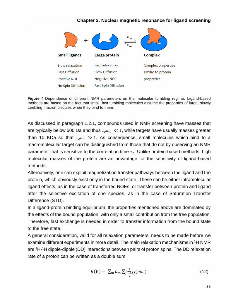
igand-based methods are based on the dependence of different NMR parameters
on the tumbling regime of the molecule studied. Molecules with 𝜏𝑐𝜔0 ≪ 1, where
𝜏𝑐 is the correlation time and 𝜔0 the Larmor frequency, have relatively long
relaxation times, large translational diffusion coefficients and positive NOEs. If such
molecules bind to a slow tumbling molecule, so that 𝜏𝑐𝜔0 ≫ 1, their behavior will change:
they will assume the properties of the slow tumbling molecule, thus having shorter
relaxation times, small translational diffusion coefficients and negative NOEs.
L
Chapter 2. Nuclear magnetic resonance for ligand screening
33
Figure 4 Dependence of different NMR parameters on the molecular tumbling regime. Ligand-based methods are based on the fact that small, fast tumbling molecules assume the properties of large, slowly tumbling macromolecules when they bind to them.
As discussed in paragraph 1.2.1, compounds used in NMR screening have masses that
are typically below 500 Da and thus 𝜏𝑐𝜔0 ≪ 1, while targets have usually masses greater
than 10 KDa so that 𝜏𝑐𝜔0 ≫ 1. As consequence, small molecules which bind to a
macromolecular target can be distinguished from those that do not by observing an NMR
parameter that is sensitive to the correlation time 𝜏𝑐. Unlike protein-based methods, high
molecular masses of the protein are an advantage for the sensitivity of ligand-based
methods.
Alternatively, one can exploit magnetization transfer pathways between the ligand and the
protein, which obviously exist only in the bound state. These can be either intramolecular
ligand effects, as in the case of transferred NOEs, or transfer between protein and ligand
after the selective excitation of one species, as in the case of Saturation Transfer
Difference (STD).
In a ligand-protein binding equilibrium, the properties mentioned above are dominated by
the effects of the bound population, with only a small contribution from the free population.
Therefore, fast exchange is needed in order to transfer information from the bound state
to the free state.
A general consideration, valid for all relaxation parameters, needs to be made before we
examine different experiments in more detail. The main relaxation mechanisms in 1H NMR
are 1H-1H dipole-dipole (DD) interactions between pairs of proton spins. The DD relaxation
rate of a proton can be written as a double sum
𝑅(𝑉) = ∑ 𝑎𝑚𝑚 ∑1
𝑟𝑗6 𝐽𝑗(𝑚𝜔)𝑗 (12)

2.5 Ligand-Based Methods
34
where the inner sum runs over all protons j that have dipolar interactions with the proton
under investigation, while the outer sum represents a linear combination of the spectral
density functions 𝐽𝑗(𝑚𝜔) evaluated at different multiples m of the Larmor frequency 𝜔.
The coefficients 𝑎𝑚 depend on the spin order 𝑉 (e.g., Iz, Ix, multiple quantum coherences,
etc.) and on the rate constant considered (e.g. R1, R2, etc.). Each spectral density 𝐽𝑗(𝜔)
can be defined as
𝐽(𝜔) =
2
5
𝜏𝑐
1 + (𝜔𝜏𝑐)2 (13)
The spectral density function 𝐽(𝜔) at 𝜔 = 0 is
𝐽(0) = 2
5𝜏𝑐 (14)
Relaxation rates that strongly depend on 𝐽(0) are highly sensitive probes for binding, since
𝜏𝑐 increases drastically upon binding, thus leading to an amplification of the corresponding
relaxation rate.
The following paragraphs will explore different commonly used methods, starting from
relaxation-filtered experiments and concluding with magnetization transfer-based
experiments.
2.5.1 Transverse Relaxation Rates
The transverse relaxation rate 𝑅2 = 1 𝑇2⁄ is perhaps the best-established NMR assay. In
fact, the strong dependence of 𝑅2 on the overall molecular rotational correlation time 𝜏𝑐
causes the difference between its values in the free and the bound form to be particularly
large. This is due to the strong dependence on 𝐽(0). Indeed R2 of a proton under 1H-1H
DD relaxation can be defined as
𝑅2 =
ℏ2𝛾𝐻4
8∑
1
𝑟𝑗6 {5𝐽𝑗(0) + 9𝐽𝑗(𝜔𝐻) + 6𝐽𝑗(2𝜔𝐻)}𝑁
𝑗=1 (15)

Chapter 2. Nuclear magnetic resonance for ligand screening
35
As a result, when the ligand is bound to the protein, one has 𝑅2,𝑏𝑜𝑢𝑛𝑑 ≫ 𝑅2,𝑓𝑟𝑒𝑒, since
𝜏𝑐,𝑐𝑜𝑚𝑝𝑙𝑒𝑥 ≫ 𝜏𝑐,𝑓𝑟𝑒𝑒 𝑙𝑖𝑔𝑎𝑛𝑑. Fast exchange allows the transfer of information from the bound
to the free state, so that the observed transverse relaxation rate 𝑅2,𝑜𝑏𝑠 can be defined as
in equation 9:
𝑅2,𝑜𝑏𝑠 = 𝑝𝐵𝑅2,𝑏𝑜𝑢𝑛𝑑 + 𝑝𝐹𝑅2,𝑓𝑟𝑒𝑒 + 𝑅𝑒𝑥 (16)
where 𝑅𝑒𝑥 is
𝑅𝑒𝑥 = (Ω𝐹 − Ω𝐵)2 𝑝𝐹𝑝𝐵
𝑘𝑒𝑥 (17)
In order to detect binding, 𝑅2,𝑜𝑏𝑠 obviously needs to be different from 𝑅2,𝑓𝑟𝑒𝑒. This means
that 𝑝𝐵𝑅2,𝑏𝑜𝑢𝑛𝑑 needs to be significant relative to 𝑝𝐹𝑅2,𝑓𝑟𝑒𝑒. However, under conditions
typical for ligand-based methods, the ligand is present in large excess ([𝐿]𝑡𝑜𝑡 [𝑃]𝑡𝑜𝑡 ≫ 1⁄ ),
so that 𝑝𝐵 is much smaller than 𝑝𝐹. Nevertheless, thanks to its 𝐽(0) dependence,
𝑅2,𝑏𝑜𝑢𝑛𝑑 ≫ 𝑅2,𝑓𝑟𝑒𝑒. As consequence, 𝑝𝐵𝑅2,𝑏𝑜𝑢𝑛𝑑 can be significant despite the large
excess of the ligand.
The rate 𝑅𝑒𝑥 expresses the line broadening due to the difference between the chemical
shifts of the free and bound states. In some circumstances, 𝑅𝑒𝑥 may be very large, so that
effects of binding on 𝑅2,𝑜𝑏𝑠 can be observed even if 𝑝𝐵𝑅2,𝑏𝑜𝑢𝑛𝑑 is not significant. In
particular, 𝑅𝑒𝑥 may be large if 𝑘𝑒𝑥 is small and/or if the difference (Ω𝐹 − Ω𝐵) between the
chemical shifts of the free and bound forms is large. The latter case is common in 19F
NMR, due to the large range of chemical shifts of fluorine.
The linewidth of a resonance is proportional to 𝑅2. If one neglects contributions due to
field inhomogeneities, etc., the linewidth in Hz can be defined as 𝐿𝑊 = 𝑅2 𝜋⁄ . As
consequence, binding events can in principle be detected by comparing the linewidths of
a small molecule in the presence and absence of a protein. In practice, if the effect is small
or if spectral crowding hampers direct comparison of the two spectra, direct observation
of line broadening can be difficult.
Alternatively, it is possible to use 𝑅2 experiments designed to observe differences in
transverse relaxation behavior in the presence and absence of a protein.[15] Typically, 𝑅2
relaxation can be monitored using Carr-Purcell-Meiboom-Gill (CPMG) pulse trains [16,
17] or continuous-wave irradiation as in 𝑅1𝜌 spin-lock methods.[18] In such experiments,

2.5.1 Transverse Relaxation Rates
36
the presence of a radiofrequency irradiation during the transverse relaxation period leads
to different expressions for 𝑅𝑒𝑥:
𝑅𝑒𝑥
𝐶𝑃𝑀𝐺 = 𝑝𝐹𝑝𝐵(Ω𝐹− Ω𝐵)2
𝑘𝑒𝑥 (1 −
2tanh (𝑘𝑒𝑥 𝑡𝑐𝑝⁄ )
𝑘𝑒𝑥𝑡𝑐𝑝) (18)
𝑅𝑒𝑥
1𝜌=
𝑝𝐹𝑝𝐵(Ω𝐹− Ω𝐵)2(sin Θ𝑟𝑓)2
𝑘𝑒𝑥 (
𝑘𝑒𝑥
(𝑘𝑒𝑥)2+ (Ω𝑆𝐿)2) (19)
where 𝑡𝑐𝑝 is the delay between two consecutive 180º pulses and Ω𝑆𝐿 is the carrier
frequency of the spin lock. In 𝑅1𝜌 experiments, on-resonance spin locking correspond to
the spin magnetization locked by the RF field along the x- or y-axis, so that 𝑅1𝜌 ≈ 𝑅2. In
both cases, comparison of 𝑅2-filtered experiments acquired with and without protein
reveals binding through one or several resonances that have been attenuated because of
an increase of 𝑅2 upon binding.
2.5.2 Paramagnetic relaxation enhancement
A variation of relaxation filtering is the approach called SLAPSTIC (spin labels attached
to protein side chains as a tool to identify interacting compounds).[19] This method
involves the use of a spin label, such as 2,2,6,6-tetramethyl-1-piperidine-1-oxyl (TEMPO),
which is covalently attached to selected protein side chains. Ligands that bind in the
proximity of the spin label will relax more rapidly, because of the electron-proton DD
interaction with the unpaired electron of the radical.
The observed transverse relaxation rate 𝑅2,𝑜𝑏𝑠 can be written as follows:
𝑅2,𝑜𝑏𝑠 = 𝑝𝐵𝑅2,𝑝𝑎𝑟𝑎 + 𝑝𝐵𝑅2,0𝐵 + 𝑝𝐹𝑅2,0𝐹 + 𝑅𝑒𝑥 (20)
where 𝑅2,𝑝𝑎𝑟𝑎 is
𝑅2,𝑝𝑎𝑟𝑎 =
ℏ2𝛾𝑒2𝛾𝐻
2
8∑
1
𝑟𝑗6
𝑁𝑗=1 {4𝐽𝑗(0) + 3𝐽𝑗(𝜔𝐻)} (21)
The j sum runs over all N spin labels in the proximity of the proton under consideration.
The electron gyromagnetic ratio 𝛾𝑒 is about 660 times larger than 𝛾𝐻. As consequence,

Chapter 2. Nuclear magnetic resonance for ligand screening
37
electron-proton DD interactions can give a huge contribution to relaxation. The large
𝑅2,𝑝𝑎𝑟𝑎 in the bound state assures that the contribution of the bound form to the 𝑅2,𝑜𝑏𝑠 is
significant, since 𝑝𝐵𝑅2,𝐵 ≫ 𝑝𝐹𝑅2,𝐹 (where 𝑅2,𝐵 is the sum of the contributions of the
paramagnetic relaxation rate 𝑅2,𝑝𝑎𝑟𝑎 and of 𝑅2,0𝐵 due to all other relaxation mechanisms).
As consequence, small fractions 𝑝𝐵 of bound ligands can be used. In some
circumstances, the use of spin labels can lead to the reduction on the order of 50 times of
the required protein concentration.[19]
For this approach to be successful, the target of interest should have amino acids that are
amenable to spin labeling (for instance lysine, tyrosine, cysteine, histidine, and
methionine) in the vicinity of the binding site. Moreover, target tailoring should not
significantly modify the structure and the flexibility of the macromolecule, since the
accidental occlusion of the site of interest would preclude binding. As consequence, prior
knowledge of the 3D structure of the protein is required.
2.5.3 Longitudinal relaxation rates
The longitudinal relaxation rate 𝑅1 = 1/𝑇1 is another parameter that is sensitive to the
correlation time. When a small molecule is interacting with a macromolecular protein, the
observed longitudinal relaxation rate 𝑅1,𝑜𝑏𝑠 can be defined as
𝑅1,𝑜𝑏𝑠 = 𝑝𝐵𝑅1,𝑏𝑜𝑢𝑛𝑑 + 𝑝𝐹𝑅1,𝑓𝑟𝑒𝑒 (22)
where 𝑅1,𝑏𝑜𝑢𝑛𝑑 and 𝑅1,𝑓𝑟𝑒𝑒 are the longitudinal relaxation rates in the bound and free
states, respectively.
It is necessary to distinguish between non-selective relaxation rates 𝑅1,𝑛𝑠 and selective
relaxation rates 𝑅1,𝑠; the former can be measured by inverting all resonances contained
in a spectrum, while the latter is determined by selectively inverting only one resonance.
The corresponding relaxation rates due to dipolar interactions between a proton i under
investigation and neighboring protons j can be defined in terms of spectral densities [20]:
𝑅1,𝑛𝑠 =
ℏ2𝛾𝐻4
10∑
1
𝑟𝑗6 {
3𝜏𝑐
1+𝜔2𝜏𝑐2 +
12𝜏𝑐
1+4𝜔2𝜏𝑐2}𝑁
𝑗=1 (23)

2.5.3 Longitudinal Relaxation Rates
38
𝑅1,𝑠 =
ℏ2𝛾𝐻4
10∑
1
𝑟𝑗6 {
3𝜏𝑐
1+𝜔2𝜏𝑐2 +
6𝜏𝑐
1+4𝜔2𝜏𝑐2 + 𝜏𝑐}𝑁
𝑗=1 (24)
The last term of equation 24 indicates a direct dependance of 𝑅1,𝑠 on 𝐽(0). Figure 5 shows
the selective and non-selective longitudinal and transverse relaxation rates as a function
of the correlation time 𝜏𝑐. One can distinguish between slow tumbing regime (𝜔𝜏𝑐 < 1),
where 𝑅1,𝑛𝑠 is smaller than 𝑅1,𝑠, and fast tumbing regime (𝜔𝜏𝑐 > 1), where 𝑅1,𝑛𝑠 > 𝑅1,𝑠.
Anyway, 𝑅1,𝑛𝑠 does not show a direct dependence on 𝜏𝑐 [21]: when a small molecule binds
to a large macromolecule, its 𝑅1,𝑠 increase rapidly, while 𝑅1,𝑛𝑠 does not.
Figure 5 𝑅1,𝑛𝑠, 𝑅1,𝑠 and 𝑅2 as a function of the correlation time. All rates were divided by the constant 𝐾 =
ℏ2𝛾𝐻4 10⁄ ∑ 1 𝑟𝑗
6⁄𝑁𝑗=1 . These simulations were performed for a Larmor frequency 𝜔 = 400 𝑀𝐻𝑧.
While testing mixtures of several compounds, it can be challenging to perturb several
chosen spins selectively. Indeed, different selective inversion pulses may have to be
applied for each compound. However, this difficulty can be circumvented by selectively
inverting a single resonance of a suitable spy molecule in competition experiments.

Chapter 2. Nuclear magnetic resonance for ligand screening
39
2.5.4 Transverse 19F relaxation
Most methods that are used for ligand-target interaction studies are based on proton
detection. Nevertheless, a few methods exploit the favorable properties of fluorine NMR
spectroscopy. Fluorine detection offers some unique advantages: (a) high sensitivity
(𝛾 𝐹19 𝛾 𝐻1⁄ = 0.94) and 100% natural abundance of the 19F isotope; (b) no interference of
signals due to non-fluorinated solvents, buffers or detergents; (c) absence of overlap with
signals of other non-fluorinated species in solution; (d) high sensitivity of the transverse
relaxation rate 𝑅2 to binding events.
Point (d) deserves to be discussed in more detail. There are two main reasons that explain
the high sensitivity of fluorine 𝑅2 to binding events: (i) the contribution of 𝐽(0) for the DD
interactions and for the chemical shift anisotropy (CSA) and (ii) the important contributions
of exchange broadening.
Fluorine transverse relaxation 𝑅2 is dominated by large contributions due to DD
interactions with proton spins in the surrounding, and CSA. For fluorine, 𝑅2 can be defined:
𝑅2 = 𝑅2𝐷𝐷 + 𝑅2
𝐶𝑆𝐴 + 𝑅2𝑜𝑡ℎ𝑒𝑟𝑠 (25)
where 𝑅2𝐷𝐷 is the contribution of the DD interactions between the isolated 19F nucleus and
surrounding protons on the ligand (and on the protein in the complex), 𝑅2𝐶𝑆𝐴 is the
contribution of CSA, and 𝑅2𝑜𝑡ℎ𝑒𝑟𝑠 stems from other sources. The rates 𝑅2
𝐷𝐷 and 𝑅2𝐶𝑆𝐴can
be defined as follows [20, 22]
𝑅2
𝐷𝐷 = 𝛾𝐹
2𝛾𝐻2 ℏ2𝜏𝑐
20∑
1
𝑟𝐹𝐻𝑖6 {4 +
1
1+(𝜔𝐹−𝜔𝐻)2𝜏𝑐2 +
3
1+𝜔𝐹2𝜏𝑐
2 +6
1+𝜔𝐻2 𝜏𝑐
2 +6
1+(𝜔𝐹+𝜔𝐻)2𝜏𝑐2}𝐻𝑖
(26)
𝑅2
𝐶𝑆𝐴 = 2
15 Δ𝜎2 (1 +
𝜂𝐶𝑆𝐴2
3) 𝜔𝐹
2𝜏𝑐 {2
3+
1
2(1+𝜔𝐹2𝜏𝑐
2)} (27)
where Δ𝜎 is the CSA of the 19F nucleus which can be defined as Δ𝜎 = 𝜎𝑧𝑧 − (𝜎𝑥𝑥+𝜎𝑦𝑦)/2,
where 𝜎𝑥𝑥, 𝜎𝑦𝑦 and 𝜎𝑧𝑧 are the principal components of the chemical shift tensor. The
asymmetry parameter is defined as 𝜂𝐶𝑆𝐴 = (3 2⁄ )(𝜎𝑥𝑥−𝜎𝑦𝑦)/Δ𝜎.
The trends of the dipolar and CSA contributions to 𝑅2 as a function of the correlation time
𝜏𝑐 are shown in figures 6 and 7, respectively. Both of these contributions are monotonic

2.5.4 Transverse 19F relaxation
40
functions of 𝜏𝑐 and can be used for screening small molecules that interact with a protein.
The relaxation of the bound state is further boosted by additional intermolecular dipolar
interactions between the 19F under investigation and protons of the macromolecular
target.
Proteins that have been selectively labeled with fluorinated amino acids have been
studied by 19F NMR since the 1970s. However, the initial results were disappointing: large
CSA effects lead to extensive line broadening of the 19F NMR spectra [23]. This fact is
well described by figure 7; the slower the molecular tumbling, the larger the CSA
contribution to the transverse relaxation. Despite the negative consequences for the
quality of the 19F spectrum of the protein, this effect turns out to be useful for detecting
binding events [24, 25]. Because of the strong dependence of CSA contributions on the
correlation time, large differences occur between the transverse relaxation rates of the
free and bound states, allowing one to detect very small fractions of ligands in the bound
state.
Figure 6 𝑅2𝐷𝐷 of 19F as a function of the correlation time. The rates were divided by the constant 𝐾 =
ℏ2𝛾𝐻2𝛾𝐹
2 𝑟𝐹𝐻𝑖
6⁄ . These simulations were performed for fluorine and proton Larmor frequencies
376 and 400 𝑀𝐻𝑧, respectively.

Chapter 2. Nuclear magnetic resonance for ligand screening
41
Figure 7 𝑅2𝐶𝑆𝐴 of 19F as a function of the correlation time. The simulations were performed for a fluorine
Larmor frequency 376 MHz. Typical CSA values of fluorobenzene were used (𝛥𝜎 = 71.5 ppm and 𝜂𝐶𝑆𝐴 = −1.32).
The transverse relaxation rates 𝑅2 of 19F are also extremely sensitive to chemical
exchange. If the relaxation rate behavior is studied through a CPMG experiment, the
observed transverse relaxation rate can be expressed as:
𝑅2,𝑜𝑏𝑠 = 𝑝𝐵𝑅2,𝑏𝑜𝑢𝑛𝑑 + 𝑝𝐹𝑅2,𝑓𝑟𝑒𝑒 + 𝑝𝐵𝑝𝐹
2𝜏𝑟𝑒𝑠4𝜋2(𝛿𝑓 − 𝛿𝑏)2 {1 − [𝑝𝐹tanh (
𝜏
𝑝𝐹𝜏𝑟𝑒𝑠)
𝜏
𝜏𝑟𝑒𝑠
]} (28)
where 𝛿𝑓 and 𝛿𝑏 are the chemical shifts of the spin under investigation in the free and
bound state, respectively, while 𝜏𝑟𝑒𝑠 = 1/𝑘𝑜𝑓𝑓 is the residence time of the ligand in the
bound state and 𝜏 is the spin-echo delay in the CPMG scheme. Simulations show that the
exchange term of equation 28 reaches its maximum value of 𝑅𝑒𝑥 = 𝑝𝐵𝑝𝐹2𝜏𝑟𝑒𝑠4𝜋2(𝛿𝑓 −
𝛿𝑏)2 for 2𝜏 ≫ 𝜏𝑟𝑒𝑠, with the 80 % of the maximum value reached with 𝜏 ≈ 5 𝜏𝑟𝑒𝑠.[26]
Indeed, if 2𝜏 is smaller than the residence time, the dephasing resulting from the exchange
can be neglected. Conversely, if 2𝜏 is larger than 𝜏𝑟𝑒𝑠, the ligand exchanges many times
between free and bound state and this will lead to maximum dephasing. This effect is
evident in figure 8. The four intensities represented in the picture are the result of four 19F
CPMG experiments with a constant total relaxation period of 80 ms, with two different 𝜏

2.5.4 Transverse 19F relaxation
42
values (left and right). In absence of protein, different spin-echo delays do not lead to
different intensities (bottom part); conversely, if exchange events occur, the exchange
contribution described above leads to a significant difference of intensities between the
two experiments.
Figure 8 19F CPMG spectra of a CF3 containing ligand in the presence (top) and absence (bottom) of a protein, recorded with two different 𝜏 values (200 µs on the left, 10 ms on the right). The difference in
intensities between experiments performed with different 𝜏 values is noticeable only in presence of the protein, when the exchange term influences the observed relaxation rate. Reproduced from [26].
2.5.5 Translational diffusion
Diffusion experiments typically use a spin echo pulse sequence with a magnetic field
gradient applied during the spin-echo delays. Before the refocusing pulse, the gradient
spatially encodes the nuclear spins, while the one after the refocusing pulse decodes
them. Only spins that do not move during the interval between the gradients will contribute
to the signal. It is possible to measure translational diffusion coefficients by incrementing
either the gradient strength or its duration.
The translational diffusion rate 𝐷 of a sphere of radius 𝑟 in a continuous medium of
viscosity 𝜂 can be defined by the Stokes-Einstein equation, [27] 𝐷 = (𝐾𝑇)/(6𝜋𝜂𝑟), where
𝐾 is the Boltzmann constant and 𝑇 is the temperature. Of course, the translational diffusion

Chapter 2. Nuclear magnetic resonance for ligand screening
43
coefficient 𝐷 is closely related to the molecular size. A large molecule will diffuse slower
than a small one.
In order to be able to apply the fast exchange approximation, the ligand needs to be in
fast exchange not only on the time scales of the chemical shifts but also on the timescale
of the diffusion measurement (typically a few hundred milliseconds) [28]. If this is the case,
the observed translational diffusion coefficient 𝐷𝑜𝑏𝑠 is:
𝐷𝑜𝑏𝑠 = 𝑝𝐵𝐷𝑏𝑜𝑢𝑛𝑑 + 𝑝𝐹𝐷𝑓𝑟𝑒𝑒 (29)
where, as usual, 𝐷𝑏𝑜𝑢𝑛𝑑 and 𝐷𝑓𝑟𝑒𝑒 are the translational diffusion constants of the bound
and free state, respectively.
Diffusion-based filtering was one of the first proposed ligand-based methods.[15] Despite
this, it has not proved to be as generally applicable as some other methods. This is mainly
due to the limited dynamic range of 𝐷, which usually differs only about one order of
magnitude between free and bound states. As consequence, low ligand-protein ratios are
required to achieve substantial changes of 𝐷𝑜𝑏𝑠 upon binding. Under these conditions,
rapid relaxation can lead to significant line broadening; as a result, this method is usually
applied to small and intermediate size proteins, which are highly soluble and available in
large amounts.
2.5.6 Transferred NOEs
There is a huge difference in correlation times between small molecules and
macromolecular proteins, with 𝜏𝑐 values in the region of 10-12 and 10-8 s, respectively.[29]
Slowly tumbling molecules show strong negative NOEs, while rapidly tumbling molecules
have weak positive NOEs. In the presence of a binding event, the small ligand acquires
transiently the correlation time of the protein, thus showing NOE cross-peaks that change
sign in 2D-NOESY.[30] Transferred NOEs are easily distinguishable from NOEs due to
the ligand in the free state, since the latter have opposite sign, and are slower to build in
intensity.
The transferred Nuclear Overhauser Effect Spectroscopy (trNOESY) experiment relies on
relatively short mixing times (100-500 ms) to probe for binding-induced changes in intra-
ligand magnetization transfer. Indeed, the mixing time should be long enough to allow the
trNOE to build up, but short enough to have negligible NOE intensities due to the free

2.5.6 Transferred NOEs
44
population. This limits the sensitivity of the method: the same binding information can be
obtained from a 1D STD experiment in 0.5 h as from a 2D trNOESY experiment in 4 h.[8]
Consequently, this method has been progressively supplanted by other methods as STD
or waterLOGSY.
Despite this, the change in sign of trNOEs makes this method useful when other screening
strategies give ambiguous results. trNOEs have proven to be extremely useful in giving
information about the bound conformation to assist modeling [31, 32], when a 3D structure
of the ligand-protein complex cannot be obtained.
An important variant of the method is the inter-ligand trNOE (ILNOE) [33], where the
trNOE is detected between two different ligands that bind to a protein in proximal sites.
This strategy can be important to extend the SAR by NMR approach to systems which
are difficult to crystallize, since it gives indications about the relative proximity of the
ligands involved in the generation of the trNOE effect.
2.5.7 NOE pumping
The previously described trNOE effects are based on intra-ligand magnetization transfer.
Alternatively, one can exploit inter-molecular NOE pathways between ligand and protein
as a signature of binding events.
In NOE pumping experiments [34], the magnetization of a small molecule is selectively
saturated by a diffusion filter, while the protein magnetization remains unchanged. A
subsequent mixing period allows a magnetization transfer from the protein to the ligand.
An additional CPMG filter can then be used in order to filter out the residual protein signals.
The method can suffer from a lack of sensitivity due to the fact that the magnetization is
stored on the macromolecular protein and its short transverse relaxation times 𝑇2 can
result in rapid losses of magnetization. A solution to this problem is provided by an inverse
experiment, where the magnetization is transferred from the ligand to the protein. This
experiment is known as reverse NOE pumping [35] and uses a CPMG filter to saturate
the protein magnetization. The magnetization stored on the ligand is then transferred to
the macromolecule during a mixing period. The result is a reduction in intensity of the
ligand signals, which would not occur in the absence of a macromolecular protein. In order
to discriminate signal losses due to NOE effects from losses due to ligand relaxation, the
experiment is performed twice: in a reference experiment, a CPMG filter is inserted after
the mixing period. In this latter experiment, the protein magnetization has not been

Chapter 2. Nuclear magnetic resonance for ligand screening
45
saturated and the ligand signals do not suffer from intensity losses due to magnetization
transfer to the macromolecule.
2.5.8 Saturation Transfer Difference
The idea of saturation transfer was already developed in the early 1960s.[36] This
approach has been applied in the late 1990s to identify binding events between small
molecules and biological targets, and has become known as Saturation Transfer
Difference (STD).[37, 38] The method exploits the magnetization transfer between an
irradiated protein and a bound ligand. The identification of the binding molecule is obtained
through the analysis of the difference between two experiments performed with or without
saturation.
In the ‘on-resonance’ experiment, a train of shaped pulses (typically N repetitions of 50
ms frequency-selective pulses with Gaussian or Seduce-1 profiles) saturates some
resonances of the protein. To selectively saturate only the protein, the irradiation is limited
to a frequency range that contains only protein resonances; usually a region shifted upfield
(between 0 and -1 ppm, containing resonances of methyl groups of the protein) or
downfield (9-10 ppm). Only a small subset of the protons of the protein is saturated by the
pulse train, but 1H-1H cross-relaxation pathways rapidly transfer this saturation across the
protein. After saturation, which usually goes on for a few seconds, a 𝜋 2⁄ pulse can be
followed by a CPMG filter to suppress the protein signals and by a water suppression
sequence to remove solvent resonances. If a small molecule binds to the protein, some
magnetization transfer will also occur at the ligand-protein interface, via intermolecular DD
interactions between protein and ligand. This will result in the partial saturation of the
ligand resonances.
In the ‘off-resonance’ experiment, the same experiment described above is performed,
but the pulse train is applied far from the protein resonances. In this case, none of the
magnetization transfer pathways described before can occur. The signals of the on-
resonance experiment are then subtracted from those of the off-resonance experiment,
usually by interleaving scans and using an inversion of the receiver phase on alternate
scans. In the resulting difference spectrum, only resonances which experienced saturation
(by direct irradiation or via magnetization transfer) will appear, thus identifying the
interacting ligand.
The STD amplification factor 𝑆𝑇𝐷𝑎𝑓 can be defined as following:

2.5.8 Saturation Transfer Difference
46
𝑆𝑇𝐷𝑎𝑓 = (𝐼0− 𝐼𝑠𝑎𝑡)
𝐼0∗
[𝐿]𝑡𝑜𝑡
[𝑃]𝑡𝑜𝑡 (30)
where 𝐼0 and 𝐼𝑠𝑎𝑡 are the signal intensities in the off- and on-resonance experiments,
respectively. Important structural information can be obtained from a detailed analysis of
the amplification factors of individual signals of the ligand. It may be possible to discern
the ligand surface that is in contact with the target (epitope mapping).[39]
Titration experiments based on the STD effect allow one to determine the dissociation
constant 𝐾𝐷 of the ligand. When 𝑆𝑇𝐷𝑎𝑓 is plotted against the total ligand concentration
[𝐿]𝑡𝑜𝑡, the curve can be fitted to the following equation to extrapolate 𝐾𝐷:
𝑆𝑇𝐷𝑎𝑓 =
−𝑆𝑇𝐷𝑎𝑓𝑚𝑎𝑥
1+([𝐿]𝑡𝑜𝑡
𝐾𝐷)
+ 𝑆𝑇𝐷𝑎𝑓𝑚𝑎𝑥 (31)
where 𝑆𝑇𝐷𝑎𝑓𝑚𝑎𝑥 is the maximum 𝑆𝑇𝐷𝑎𝑓 effect.
The STD method has some unique advantages. First of all, the technique works
particularly well with high-molecular mass drug targets, since efficient spin diffusion within
the protein is needed in order to transfer the magnetization to the bound ligand. Moreover,
in systems where fast exchange prevails, slow relaxation of the ligand in its free state
allows one to accumulate a high concentration of saturated ligand molecules over the
duration of the saturating pulse train. This permits to saturate large amounts of ligand with
low concentrations of protein. As consequence, STD experiments can be performed with
a 50-500-fold excess of ligand.
The NOE cross-relaxation 𝜎𝑁𝑂𝐸 rate between two protons depends on the correlation time
𝜏𝑐:
𝜎𝑁𝑂𝐸 = 𝛾4ℏ2
10𝑟𝑖𝑗6 {
6𝜏𝑐
1+4𝜔2𝜏𝑐2 − 𝜏𝑐} (32)
In the presence of small or medium-sized proteins with a relatively small 𝜏𝑐, magnetization
transfer via DD interactions may be inefficient, so that the complete saturation of the
protein may fail. Moreover, the observed 𝑆𝑇𝐷𝑎𝑓 cannot be linked directly to the affinity of
a ligand: a strong binder will show weak STD signals since a small 𝑘𝑜𝑓𝑓 limits the turnover
of ligand molecules in the binding site. Another problem can be saturation leakage [40]
Chapter 2. Nuclear magnetic resonance for ligand screening
47
via chemical exchange with the solvent; for this reason the STD experiment is
preferentially performed in D2O rather than H2O. Nucleic acid proteins suffer from a low
proton density which limits cross-relaxation within the protein, so that the STD technique
is not very useful for this kind of systems.
The epitope mapping from the analysis of 𝑆𝑇𝐷𝑎𝑓 of ligand signals can only be performed
for binders with weak affinities. Indeed, if the residence time is long compared to cross-
relaxation of the ligand in the bound state, the magnetization spreads over all ligand
protons and leads to a uniformly small STD effect.[21]
STD technique is useful for the study of ligands with 10−8 < 𝐾𝐷 < 10−3 M.[37] For weaker
ligands and if [𝐿]𝑡𝑜𝑡 < 𝐾𝐷, less than half of the protein molecules will be bound to a ligand.
This means that the saturation transfer from the protein to the ligand is inefficient.
Conversely, for stronger ligands, the kinetic off-rate constant 𝑘𝑜𝑓𝑓 is very small, thus
diminishing the saturation of the magnetization on the ligand. In particular, if the residence
time of the ligand in the bound state is long on the timescale of its 𝑅1 in the bound state,
the ligand cannot “remember” its visit to the binding site of the saturated protein and
relaxes back to equilibrium.
2.5.9 WaterLOGSY
The NOE pumping and STD methods described in the previous two paragraphs rely on
the selective perturbation of the magnetization of either ligand or protein and exploit the
magnetization transfer between the two species to characterize the binding properties of
the molecule under investigation. The so-called “water-ligand observed via gradient
spectroscopy” (water-LOGSY) method [41] represents an elegant modification of these
approaches.
WaterLOGSY does not need to create a pool of magnetization on either ligand or protein.
It is based on indirect excitation of the magnetization of the ligand-protein complex and of
the free ligand by selective perturbation of bulk water magnetization. The perturbation of
bulk water can be achieved either by selective saturation or by selective inversion of the
water signal. Nowadays, the most robust scheme to achieve efficient selective inversion
of the water signal is ePHOGSY,[42, 43] which consists of a water-selective 180º
refocusing pulse sandwiched between two pulsed field gradients.
Different pathways can be involved in the transfer of magnetization from bulk water to
either bound or free ligand molecules. Bound ligand molecules benefit from magnetization

2.5.9 WaterLOGSY
48
transfer from water molecules that reside in the binding site and in the hydration sphere
around the ligand-protein complex. Moreover, chemical exchange between bulk water and
exchangeable protons of the protein, i.e., labile carboxyl, amino, hydroxyl, imidazole,
guanidinium and amide protons [44, 45], pumps protein magnetization that can be
transferred to the ligand. When the ligands are bound to the protein, the magnetization
transfer within the ligand-protein complex occurs rapidly because of its long correlation
time 𝜏𝑐, generating large negative signals.
In the waterLOGSY experiment, magnetization is also transferred directly from the bulk
water to the free ligand molecules. This transfer occurs via DD interactions between the
hydration shell and the free ligand molecule, and possibly via chemical exchange through
exchangeable protons of the ligand. In this case, the DD interactions fluctuate with short
correlation times, leading to weak positive NOE’s that generate small positive signals. The
spectra are usually shown phased so that bound signals are positive and free signals
negative. As consequence, the observed waterLOGSY signals 𝐼𝑊𝐿 result from the sum of
negative signals due to free ligands that cannot bind and positive signals of ligand
molecules that can bind to the protein [8]:
𝐼𝑊𝐿 = 𝐶([𝑃𝐿]𝜎𝑏𝑜𝑢𝑛𝑑 + [𝐿]𝜎𝑓𝑟𝑒𝑒) (33)
Where C is a proportionality constant that accounts for the appropriate unit conversions,
[𝑃𝐿] is the concentration of the bound ligand, [𝐿] is the concentration of the free ligand,
while 𝜎𝑏𝑜𝑢𝑛𝑑 and 𝜎𝑓𝑟𝑒𝑒 are the cross-relaxation rate constants describing the transfer of
magnetization from water to ligand protons in the bound and free states, respectively.
As the contribution of the free state becomes more significant, the resulting waterLOGSY
spectrum of the ligand can pass through a null or be negative. For instance, if [𝐿]𝑡𝑜𝑡 ≫
[𝑃]𝑡𝑜𝑡 the negative contribution of the free state [𝐿]𝜎𝑓𝑟𝑒𝑒 may overwhelm that of bound
state, resulting in a false negative. For this reason, the experiment should not be carried
out with large ligand/protein ratios. The reference spectrum 𝐼𝑊𝐿,𝑓𝑟𝑒𝑒 recorded in the
absence of the protein can be subtracted from the spectrum 𝐼𝑊𝐿 obtained in the presence
of the protein. The difference 𝐼𝑊𝐿 − 𝐼𝑊𝐿,𝑓𝑟𝑒𝑒 can be defined as [8]:
𝐼𝑊𝐿 − 𝐼𝑊𝐿,𝑓𝑟𝑒𝑒 =
[𝑃]𝑡𝑜𝑡(𝜎𝑏𝑜𝑢𝑙𝑑− 𝜎𝑓𝑟𝑒𝑒)[𝐿]
[𝐿]+ 𝐾𝐷 (34)

Chapter 2. Nuclear magnetic resonance for ligand screening
49
Fitting the curve of 𝐼𝑊𝐿 − 𝐼𝑊𝐿,𝑓𝑟𝑒𝑒 during a titration to equation 34 and approximating [𝐿] ≈
[𝐿]𝑡𝑜𝑡 allows one to estimate 𝐾𝐷. The estimated lower limit of 𝐾𝐷 that can be detected is
𝐾𝐷 ≈ 0.1 µM.[46] Ligands with a greater affinity have longer residence times so that the
transferred magnetization is lost due to longitudinal relaxation before the ligand leaves the
binding site.
WaterLOGSY can be used when STD is not applicable, as for nucleic acid proteins.[47]
The bulk water can be seen as a pool of magnetization that compensates for the lack of
proton DD cross-relaxation pathways in proteins with low proton density.
Figure 9 Identification of a ligand that binds to the protein cdk2 in a mixture of 10 compounds using waterLOGSY. Top: 1H spectrum of the mixture in absence of protein. Bottom: waterLOGSY spectrum of the mixture in the presence of the protein. The positive waterLOGSY peak framed in a dashed red square indicates binding of the corresponding compound to the protein. Spectra reproduced from [21].

50
References
1. S. B. Shuker, P. J. Hajduk, R. P. Meadows, and S. W. Fesik, Discovering high-affinity ligands for proteins: SAR by NMR. Science, 1996. 274(5292): p. 1531-1534.
2. D. A. Erlanson, R. S. McDowell, and T. O'Brien, Fragment-based drug discovery. Journal of Medicinal Chemistry, 2004. 47(14): p. 3463-3482.
3. M. J. Hartshorn, C. W. Murray, A. Cleasby, M. Frederickson, I. J. Tickle, and H. Jhoti, Fragment-based lead discovery using X-ray crystallography. Journal of Medicinal Chemistry, 2005. 48(2): p. 403-413.
4. S. A. Hofstadler and R. H. Griffey, Analysis of noncovalent complexes of DNA and RNA by mass spectrometry. Chemical Reviews, 2001. 101(2): p. 377-390.
5. D. J. Maly, I. C. Choong, and J. A. Ellman, Combinatorial target-guided ligand assembly: Identification of potent subtype-selective c-Src inhibitors. Proceedings of the National Academy of Sciences of the United States of America, 2000. 97(6): p. 2419-2424.
6. R.E. Hubbard and Royal Society of Chemistry, Structure-based Drug Discovery: An Overview. 2006: Royal Society of Chemistry.
7. K.A. Connors, Binding constants: the measurement of molecular complex stability. 1987: Wiley.
8. C. A. Lepre, J. M. Moore, and J. W. Peng, Theory and applications of NMR-based screening in pharmaceutical research. Chemical Reviews, 2004. 104(8): p. 3641-3675.
9. E. L. Hahn and D. E. Maxwell, Spin Echo Measurements of Nuclear Spin Coupling in Molecules. Physical Review, 1952. 88(5): p. 1070-1084.
10. H. M. Mcconnell, Reaction Rates by Nuclear Magnetic Resonance. Journal of Chemical Physics, 1958. 28(3): p. 430-431.
11. P. J. Hajduk, M. Bures, J. Praestgaard, and S. W. Fesik, Privileged molecules for protein binding identified from NMR-based screening. Journal of Medicinal Chemistry, 2000. 43(18): p. 3443-3447.
12. P. J. Hajduk, G. Sheppard, D. G. Nettesheim, E. T. Olejniczak, S. B. Shuker, R. P. Meadows, D. H. Steinman, G. M. Carrera, P. A. Marcotte, J. Severin, K. Walter, H. Smith, E. Gubbins, R. Simmer, T. F. Holzman, D. W. Morgan, S. K. Davidsen, J. B. Summers, and S. W. Fesik, Discovery of potent nonpeptide inhibitors of
References

Chapter 2. Nuclear magnetic resonance for ligand screening
51
stromelysin using SAR by NMR. Journal of the American Chemical Society, 1997.
119(25): p. 5818-5827.
13. I. Bertini, K.S. McGreevy, and G. Parigi, NMR of Biomolecules: Towards
Mechanistic Systems Biology. 2012: Wiley.
14. W. P. Jencks, On the Attribution and Additivity of Binding-Energies. Proceedings
of the National Academy of Sciences of the United States of America-Biological
Sciences, 1981. 78(7): p. 4046-4050.
15. P. J. Hajduk, E. T. Olejniczak, and S. W. Fesik, One-dimensional relaxation- and
diffusion-edited NMR methods for screening compounds that bind to
macromolecules. Journal of the American Chemical Society, 1997. 119(50): p.
12257-12261.
16. H. Y. Carr and E. M. Purcell, Effects of Diffusion on Free Precession in Nuclear
Magnetic Resonance Experiments. Physical Review, 1954. 94(3): p. 630-638.
17. S. Meiboom and D. Gill, Modified Spin-Echo Method for Measuring Nuclear
Relaxation Times. Review of Scientific Instruments, 1958. 29(8): p. 688-691.
18. C. Deverell, R. E. Morgan, and J. H. Strange, Studies of Chemical Exchange by
Nuclear Magnetic Relaxation in Rotating Frame. Molecular Physics, 1970. 18(4):
p. 553-559.
19. W. Jahnke, S. Rudisser, and M. Zurini, Spin label enhanced NMR screening.
Journal of the American Chemical Society, 2001. 123(13): p. 3149-3150.
20. R.R. Ernst, G. Bodenhausen, and A. Wokaun, Principles of Nuclear Magnetic
Resonance in One and Two Dimensions. 1990: Clarendon Press.
21. B. J. Stockman and C. Dalvit, NMR screening techniques in drug discovery and
drug design. Progress in Nuclear Magnetic Resonance Spectroscopy, 2002. 41(3-
4): p. 187-231.
22. D. Canet, Nuclear Magnetic Resonance: Concepts and Methods. 1996: Wiley.
23. W. E. Hull and B. D. Sykes, Fluorotyrosine Alkaline-Phospatase - internal mobility
of individual tyrosines and role of chemical-shift anisotropy as a F-19 nuclear spin
relaxation mechanism in proteins. Journal of Molecular Biology, 1975. 98(1): p.
121-153.
24. C. Dalvit, M. Flocco, M. Veronesi, and B. J. Stockman, Fluorine-NMR competition
binding experiments for high-throughput screening of large compound mixtures.
Combinatorial Chemistry & High Throughput Screening, 2002. 5(8): p. 605-611.
25. C. Dalvit, P. E. Fagerness, D. T. A. Hadden, R. W. Sarver, and B. J. Stockman,
Fluorine-NMR experiments for high-throughput screening: Theoretical aspects,

References
52
practical considerations, and range of applicability. Journal of the American
Chemical Society, 2003. 125(25): p. 7696-7703.
26. C. Dalvit, Ligand- and substrate-based F-19 NMR screening: Principles and
applications to drug discovery. Progress in Nuclear Magnetic Resonance
Spectroscopy, 2007. 51(4): p. 243-I.
27. P. Stilbs, Fourier transform pulsed-gradient spin-echo studies of molecular
diffusion. Progress in Nuclear Magnetic Resonance Spectroscopy, 1987. 19: p. 1-
45.
28. L. Fielding, NMR methods for the determination of protein-ligand dissociation
constants. Progress in Nuclear Magnetic Resonance Spectroscopy, 2007. 51(4):
p. 219-242.
29. S. W. Homans, A dictionary of concepts in NMR. Rev. pbk. ed. ed. Biophysical
techniques series ;. 1992, New York :Oxford University Press: Oxford.
30. D. Neuhaus and M.P. Williamson, The Nuclear Overhauser Effect in Structural and
Conformational Analysis. 1989: VCH.
31. F. Ni, Y. Zhu, and H. A. Scheraga, Thrombin-Bound Structures of Designed
Analogs of Human Fibrinopeptide-a Determined by Quantitative Transferred Noe
Spectroscopy - a New Structural Basis for Thrombin Specificity. Journal of
Molecular Biology, 1995. 252(5): p. 656-671.
32. N. Evrard-Todeschi, J. Gharbi-Benarous, C. Gaillet, L. Verdier, G. Bertho, C. Lang,
A. Parent, and J. P. Girault, Conformations in solution and bound to bacterial
ribosomes of ketolides, HMR 3647 (telithromycin) and RU 72366: A new class of
highly potent antibacterials. Bioorganic & Medicinal Chemistry, 2000. 8(7): p. 1579-
1597.
33. D. W. Li, E. F. DeRose, and R. E. London, The inter-ligand Overhauser effect: A
powerful new NMR approach for mapping structural relationships of
macromolecular ligands. Journal of Biomolecular Nmr, 1999. 15(1): p. 71-76.
34. A. Chen and M. J. Shapiro, NOE pumping: A novel NMR technique for identification
of compounds with binding affinity to macromolecules. Journal of the American
Chemical Society, 1998. 120(39): p. 10258-10259.
35. A. D. Chen and M. J. Shapiro, NOE pumping. 2. A high-throughput method to
determine compounds with binding affinity to macromolecules by NMR. Journal of
the American Chemical Society, 2000. 122(2): p. 414-415.
36. S. Forsen and R. A. Hoffman, Study of Moderately Rapid Chemical Exchange
Reactions by Means of Nuclear Magnetic Double Resonance. Journal of Chemical
Physics, 1963. 39(11): p. 2892-&.

Chapter 2. Nuclear magnetic resonance for ligand screening
53
37. M. Mayer and B. Meyer, Characterization of ligand binding by saturation transfer
difference NMR spectroscopy. Angewandte Chemie-International Edition, 1999.
38(12): p. 1784-1788.
38. J. Klein, R. Meinecke, M. Mayer, and B. Meyer, Detecting binding affinity to
immobilized receptor proteins in compound libraries by HR-MAS STD NMR.
Journal of the American Chemical Society, 1999. 121(22): p. 5336-5337.
39. M. Mayer and B. Meyer, Group epitope mapping by saturation transfer difference
NMR to identify segments of a ligand in direct contact with a protein receptor.
Journal of the American Chemical Society, 2001. 123(25): p. 6108-6117.
40. V. Jayalakshmi and N. R. Krishna, Complete relaxation and conformational
exchange matrix (CORCEMA) analysis of intermolecular saturation transfer effects
in reversibly forming ligand-receptor complexes. Journal of Magnetic Resonance,
2002. 155(1): p. 106-118.
41. C. Dalvit, P. Pevarello, M. Tato, M. Veronesi, A. Vulpetti, and M. Sundstrom,
Identification of compounds with binding affinity to proteins via magnetization
transfer from bulk water. Journal of Biomolecular Nmr, 2000. 18(1): p. 65-68.
42. C. Dalvit, Homonuclear 1D and 2D NMR experiments for the observation of
solvent-solute interactions. Journal of Magnetic Resonance Series B, 1996. 112(3):
p. 282-288.
43. C. Dalvit, Efficient multiple-solvent suppression for the study of the interactions of
organic solvents with biomolecules. Journal of Biomolecular Nmr, 1998. 11(4): p.
437-444.
44. G. Otting and E. Liepinsh, Protein hydration viewed by high reslotuion NMR-
spectroscopy - Implications for magnetic-resonance image-contrast. Accounts of
Chemical Research, 1995. 28(4): p. 171-177.
45. E. Liepinsh and G. Otting, Proton exchange rates from amino acid side chains -
Implications for image contrast. Magnetic Resonance in Medicine, 1996. 35(1): p.
30-42.
46. C. Dalvit, G. Fogliatto, A. Stewart, M. Veronesi, and B. Stockman, WaterLOGSY
as a method for primary NMR screening: Practical aspects and range of
applicability. Journal of Biomolecular Nmr, 2001. 21(4): p. 349-359.
47. E. C. Johnson, V. A. Feher, J. W. Peng, J. M. Moore, and J. R. Williamson,
Application of NMR SHAPES screening to an RNA target. Journal of the American
Chemical Society, 2003. 125(51): p. 15724-15725.

54

Chapter 3. Nuclear Long-Lived States
55
3. Nuclear Long-Lived States
wo particles with spin I = 1/2 can couple to form a composite system with total spin
I = 0 or 1. The spin I = 0 state can only have the magnetic quantum number m =
0, while the spin I = 1 configuration comprises three distinct energy levels (m = -1,
0, 1). These two categories of spin states are called respectively singlet state and triplet
states.
When the two spin-1/2 particles are both electrons, there is usually a large energy
difference between the singlet and triplet states, mainly due to the electron exchange
interaction, which arises from the overlap of the electronic wavefunctions. In this situation,
the electronic singlet and triplet states are nearly exact eigenfunctions of the Hamiltonian
of the system. In many cases, an excited electronic singlet state is converted into lower-
energy electronic triplet states through a process known as intersystem crossing (ISC).
If the two spin-1/2 particles are both nuclei, the situation is different. Nuclear exchange
couplings are usually small, because the nuclear wavefunctions are strongly localized and
there is no overlap. Since the nuclear exchange coupling usually vanishes, the singlet-
triplet energy splitting is extremely small, and it is often dominated by weak symmetry-
breaking interactions such as the chemical shift difference. As a consequence, the use of
the language of singlet and triplet states is less widespread in NMR, compared with the
fields of electronic spectroscopy or molecular quantum mechanics. However, the
concepts of singlet and triplet states are very important to understand the relaxation
properties of the nuclear spin systems.
The singlet and triplet states of a nuclear spin-1/2 pair can be described by the
wavefunctions [1]:
|𝑆0⟩ = 1√2⁄ (|𝛼𝛽⟩ − |𝛽𝛼⟩)
|𝑇−1⟩ = |𝛽𝛽⟩
|𝑇0⟩ = 1√2⁄ (|𝛼𝛽⟩ + |𝛽𝛼⟩)
|𝑇+1⟩ = |𝛼𝛼⟩
(1)
where the symbols 𝛼 and 𝛽 refer to angular momentum components ±ℏ/2 respectively,
along a defined quantization axis (usually, the external magnetic field axis). If the system
T

3. Nuclear Long-Lived States
56
is exposed to an external magnetic field, the configuration of the energy eigenstates of
the spin-1/2 pair is different if the nuclear sites are magnetically equivalent or inequivalent.
If the nuclear sites are magnetically equivalent, the nuclei experience identical local
magnetic fields generated by the local electronic environment. In this situation, the singlet
and triplet states are exact eigenstates of the Hamiltonian of the system. The three triplet
states are split by the nuclear Zeeman resonance frequency, which is proportional to the
applied magnetic field, as shown in figure 1.
Figure 1 Energy levels for a system of two magnetically equivalent spins with I = 1/2.
If the nuclear sites are magnetically inequivalent, the nuclei experience local fields which
can be significantly different, depending on the size of the chemical shift difference and
the magnitude of the external magnetic field. If this difference is much larger than the
scalar coupling between the two spins, the spin-pair is said to be weakly coupled. In this
situation, the energy eigenstates of the system are close to the individual Zeeman states
|𝛼𝛼⟩, |𝛼𝛽⟩, |𝛽𝛼⟩ and |𝛽𝛽⟩, as shown in figure 2.
Usually, the relaxation of nuclear spin systems is described by Redfield’s equations, which
involve transition probabilities between pairs of eigenstates. The classical Redfield theory
of weakly-coupled spin pairs does not use the singlet and triplet states, since these are
not eigenstates of a system of two inequivalent spins.
However, the use of singlet and triplet states in the Redfield formalism can show an
important property: just as in electronic spectroscopy, where intersystem crossing
between singlet and triplets is a slow process, nuclear singlet-triplet transitions break spin-

Chapter 3. Nuclear Long-Lived States
57
exchange symmetry and are therefore hindered. In addition, if the coherent singlet-triplet
transitions are suppressed, the lifetime of the nuclear singlet order is often longer than the
longitudinal relaxation time 𝑇1. This fact provides the interesting possibility of storing
nuclear spin order for times much longer than 𝑇1.[2-4]
Figure 2 Energy levels for a magnetically inequivalent 2-spin-1/2 system.
However, in order to exploit these longer lifetimes, two problems must be overcome. In
the case of two inequivalent spins, spin order cannot be deposited in a state that is not an
eigenstate of the Hamiltonian of the system. Indeed, rapid singlet-triplet interconversion
would lead to a rapid depletion of the non-equilibrium state. On the other hand, singlet
states cannot be observed directly, since they have total spin zero and therefore they do
not give rise to any NMR signal.
3.1 The principle of symmetry-switching
he solution to both problems outlined above is to switch the symmetry of the spin
interactions at different points during the experimental procedure. When the
symmetry prevails, coherent singlet-triplet transitions are quenched, so that the
lifetime of the singlet state is extended. When the symmetry is broken, singlet-triplet
T

3.1 The principle of symmetry-switching
58
transitions are allowed, so that spin order to be deposited in the singlet state and be
converted into detectable magnetization.
A typical singlet NMR experiment comprises three steps:
In the excitation interval, the symmetry is broken, so that coherent singlet-triplet
transitions are allowed. These coherent transitions are used to create an imbalance
between the populations of the singlet and triplet states, abbreviated as TSI (triplet-
singlet imbalance);
In the storage interval, coherent singlet-triplet transitions are quenched by imposing
spin-exchange symmetry. During this period, the TSI decays with a time constant
𝑇𝑇𝑆𝐼 (also known as 𝑇𝑆), which may be longer than the longitudinal relaxation time
𝑇1;
In the detection interval, the symmetry is broken again. This permits the
observation of singlet-derived NMR signals. In fact, nuclear singlet order is non-
magnetic, but the broken symmetry restores coherent singlet-triplet transitions,
which are used to obtain observable nuclear magnetization.
If a pair of magnetically equivalent spins is considered, symmetry is a starting feature of
the system. The symmetry has to be broken both to populate the TSI and subsequently
during the detection interval. Conversely, if an inequivalent two-spin system is considered,
symmetry must be imposed during the storage interval.
All para-hydrogen-based methods belong to the first category and exploit the use of
chemical reactions to break the symmetry of the two magnetically equivalent spins during
the excitation and detection intervals.[5, 6] Dihydrogen gas is prepared in a metastable
state of enriched nuclear singlet order by thermal equilibration at low temperatures
(typically 40 K) in the presence of a metal catalyst, followed by separation from the catalyst
and warming to ambient temperature. The symmetry of the hydrogen molecule is usually
broken by a reaction in a metal complex. In this state of broken symmetry, coherent
singlet-triplet transitions permit the conversion of hyperpolarized singlet order to
hyperpolarized magnetization, thus leading to large NMR signals.
It has been recently demonstrated that a singlet-triplet imbalance can also be created
directly in a system of magnetically equivalent spins by dynamic nuclear polarization
(DNP); the resulting long-lived states have been nicknamed Hyperpolarized Equivalent
Long-Lived States (HELLS).[7] The detection is performed after the symmetry has been
broken, by means of enzymatic or chemical reactions. Alternatively, the TSI can be

Chapter 3. Nuclear Long-Lived States
59
transferred by cross-relaxation to observable, enhanced signals of protons and coupled 13C spins.[8]
Alternatively, many traditional methods use a change of the magnetic field to which the
nuclei are exposed to impose or remove the symmetry in a system of magnetically
inequivalent spins. In field-cycling singlet NMR, a strong magnetic field is applied to break
the exchange symmetry. Then, exchange symmetry is restored by removing this magnetic
field and coherent singlet-triplet transitions are suppressed. To obtain detectable
magnetization, radiofrequency pulse sequences can be applied at the nuclear resonance
frequency.[1, 2, 9] In high-field NMR, the nuclear singlet order is maintained by using a
resonant spin-locking field which suppresses effects of chemical shift differences and
establishes an effective spin-exchange symmetry in the nuclear spin Hamiltonian.[1, 3,
10]
3.2 Applications
he extended lifetime of nuclear singlet states can suggest new applications of
hyperpolarized NMR. In fact, they can provide a possibility to reduce losses of
hyperpolarized spin order due to relaxation in the interval between the generation
of hyperpolarized spin order and its use.
Dynamic nuclear polarization (DNP) consists in the doping of the sample with
paramagnetic species and the application of a resonant microwave field slightly offset
from the electron Larmor frequency at low temperatures. Under suitable conditions, a
large polarization of nuclei builds up. It has been shown that the frozen sample can be
dissolved using injection of a hot solvent and transferred to an NMR magnet, resulting in
an enormous increase in signal strength.[11] Nevertheless, this dissolution method (D-
DNP) has a serious limitation: hyperpolarized magnetization has a limited lifetime, which
decays with the time constant 𝑇1. Relaxation causes important losses of hyperpolarization
during the warming process, the transport to the second magnet, or the transport of the
hyperpolarized substance to the site of interest. The use of singlet states has enormous
potential in combination with dissolution-DNP. Tayler and coworkers have shown that a
TSI can be directly populated before the transfer by DNP for the two inequivalent 13C spins
in 1,2-13C2-pyruvic acid.[12] They demonstrated that a singlet-triplet population imbalance
could be created directly by hyperpolarization, i.e., without any extra manipulations of the
T

3.2 Applications
60
sample. However, in this experiment the magnitude of the TSI, which depends on the
nuclear polarization reached, was very limited. As discussed before, alternative strategies
involve the use of magnetically equivalent spin systems and particular strategies for the
detection of the otherwise NMR-silent singlet order. [7, 8] However, most of the current
experiments where D-DNP is combined with LLS rely on rf pulses sequences to prepare
the LLS after the transfer of the hyperpolarized sample to the detection spectrometer.[13-
15]
The extended lifetime of singlet states allows a greater interval for the transport to take
place, while still maintaining the memory of the nuclear spin system. This allows the
measurement of smaller diffusion coefficients or slower flow rates. Singlet states can also
allow the study of slower exchange processes than is normally the case.[4, 16, 17]
The relaxation of nuclear singlet states is sensitive to the presence of nearby magnetic
centers such as other magnetic nuclei and can therefore be used as a probe of molecular
geometry. Its sensitivity to changes in molecular structure can be used to detect protein
folding and unfolding.[18]
3.3 Long-Lived States: the principles
uclear magnetic resonance can give structural and dynamic information on
molecules containing nuclei with a non-vanishing magnetic moment.
Many studies, like the examination of slow translational diffusion, chemical
exchange or folding of proteins, are limited by the longitudinal relaxation time 𝑇1, which
gives a measure of the time needed for the nuclear spins to return to thermal equilibrium.
𝑇1 is usually regarded as the maximum lifetime of the memory of nuclear spins.
Nevertheless, Carravetta and Levitt have recently demonstrated that there are nuclear
spin states whose decay time constant 𝑇𝐿𝐿𝑆 is much longer than 𝑇1.[1, 10, 19, 20] These
nuclear states are called Long Lived States (LLS). LLS are based on peculiar properties
of singlet states, i.e., spin states that can be represented by an antisymmetric combination
of Zeeman spin states of two nuclei. A singlet state is immune to the dipolar interaction
between the two spins of the system, which is the main relaxation mechanism in solution-
state NMR. If a population imbalance between singlet and triplet states can be created, it
can be be stored for a long time.
N

Chapter 3. Nuclear Long-Lived States
61
Nuclear spin states are conveniently labeled as |𝛼⟩ and |𝛽⟩ according to the projection of
their angular moment onto the z-axis:
𝐼𝑧|𝛼⟩ = 1
2 |𝛼⟩ (2)
𝐼𝑧|𝛽⟩ = −
1
2 |𝛽⟩ (3)
Singlet and triplet states are defined as antisymmetric and symmetric superpositions,
respectively, of the Zeeman spin states. As mentioned in equation 1, they can be written
as follows:
|𝑆0⟩ = 1√2⁄ (|𝛼𝛽⟩ − |𝛽𝛼⟩)
|𝑇−1⟩ = |𝛽𝛽⟩
|𝑇0⟩ = 1√2⁄ (|𝛼𝛽⟩ + |𝛽𝛼⟩)
|𝑇+1⟩ = |𝛼𝛼⟩
with
𝐼2|𝑆0⟩ = 𝐼(𝐼 + 1)|𝑆0⟩ = 0 (4.1)
𝐼2|𝑇𝑚⟩ = 𝐼(𝐼 + 1)|𝑇𝑚⟩ = 2|𝑇𝑚⟩ (4.2)
where 𝐼2 = 𝐼𝑥2 + 𝐼𝑦
2 + 𝐼𝑧2 is the square of the spin angular momentum and 𝑚 = −1, 0, +1
is the quantum number for the projection of 𝐼 onto the quantization axis.[21]
These states can be classified according to their symmetry properties with respect to the
spin exchange operator P:
𝑷|𝑆0⟩ = −|𝑆0⟩ (5.1)

3.3 Long-Lived States: the principles
62
𝑷|𝑇𝑚⟩ = +|𝑇𝑚⟩ (5.2)
The singlet state is anti-symmetric while the triplet states are symmetric with respect to
the exchange of the two spins. The singlet and triplet states are eigenstates of the spin
Hamiltonian for a magnetically equivalent spin pair.
When the two spins are in magnetically equivalent environments, the nuclear spin
Hamiltonian can be written as follows:
𝐻 = 𝜔0𝐼𝑧 + 2𝜋𝐽𝐼1𝐼2 (6)
where 𝐽 is the spin-coupling constant, 𝜔0 = −𝛾𝐵 is the Larmor frequency and 𝐵 is the
applied static magnetic field. Its matrix representation in the singlet-triplet basis is:
|𝑆0⟩ |𝑇+1⟩ |𝑇0⟩ |𝑇−1⟩
𝐻 =
(
−3
2𝜋𝐽 0 0 0
0 𝜔0 +1
2𝜔𝐽 0 0
0 01
2𝜔𝐽 0
0 0 0 −𝜔0 +1
2𝜔𝐽)
(7)
If the two spins are in magnetically equivalent environments, the three triplet states are
spaced by energy dfferences 𝛾𝐵 and there is a field-independent energy difference of 2𝜋𝐽
between the singlet state and the central triplet state.
The singlet state is non-magnetic and does not induce any NMR signal. In practice, with
the inversion-recovery method, in a system of magnetically equivalent spin pairs, only the
relaxation to equilibrium within the triplet manifold is measured. The time constant 𝑇1 is
thus an exclusive property of the triplet states.
However, the situation is different if the population of the singlet state is perturbed with
respect to that of the triplet state. In this case, the re-establishment of thermal equilibrium

Chapter 3. Nuclear Long-Lived States
63
needs singlet-triplet transitions. Here is the heart of the phenomenon. These transitions
can be far slower than 𝑇1.
The reason why 𝑇𝑠 is usually longer that 𝑇1 can be explained by symmetry considerations.
It has been demonstrated in equation 5 that the singlet state is antisymmetric under
exchange, while the three triplet states are symmetric with respect to exchange. However,
the conversion of an exchange-antisymmetric state into an exchange-symmetric state
requires a mechanism that is itself exchange-antisymmetric. Since many of the strongest
relaxation processes are exchange-symmetric (including the homonuclear dipole-dipole
coupling between the nuclei, which is the strongest relaxation mechanism in a system of
two coupled spin-1/2 in solution), they cannot contribute to 𝑇𝑠. In general, a relaxation
mechanism can induce singlet-triplet transitions only if it does something 'different' to the
two nuclear spins.
When the two spins are in magnetically inequivalent environments, the nuclear spin
Hamiltonian can be written as follows:
𝐻 = 𝜔0(1 + 𝛿1)𝐼1𝑧 + 𝜔0(1 + 𝛿2)𝐼2𝑧 + 2𝜋𝐽𝐼1𝐼2 (8)
where 𝛿1 and 𝛿2 are the two chemical shifts. Its matrix representation in the singlet-triplet
basis is the following:
|𝑆0⟩ |𝑇+1⟩ |𝑇0⟩ |𝑇−1⟩
𝐻 =
(
−3
2𝜋𝐽 0
1
2𝜔0Δ 𝛿 0
0 𝜔0(1 +1
2Σ 𝛿) +
1
2𝜔𝐽 0 0
1
2𝜔0Δ 𝛿 0
1
2𝜔𝐽 0
0 0 0 −𝜔0(1 +1
2Σ 𝛿) +
1
2𝜔𝐽)
(9)
where the sum and the difference of the chemical shifts are:

3.3 Long-Lived States: the principles
64
Σ 𝛿 = 𝛿1 + 𝛿2 (10.1)
Δ 𝛿 = 𝛿1 − 𝛿2 (10.2)
The relaxation theory for inequivalent spin-1/2 pairs does not predict any states that have
a lifetime longer than 𝑇1. The reason is apparent in equation 9: there are two terms
12⁄ 𝜔0 Δ 𝛿 that connect the singlet state to the central triplet state. These terms indicate
that singlet-triplet transitions are induced by the chemical shift frequency difference
𝜔0 Δ 𝛿. Therefore, the long-lived nature of the singlet state is masked by the chemical shift
difference. In order to fully exploit the long lifetime of singlet states the chemical shift
difference must be suppressed.
3.4 The singlet NMR experiment
n the case of magnetically equivalent spin pairs, singlet and triplet states are
eigenstates of the spin system. However, the singlet state is non-magnetic and does
not provide an NMR signal. In the case of magnetically inequivalent spin pairs, when
the nuclear spin Hamiltonian is expressed in the singlet-triplet basis, the cross terms
between singlet and triplet states demonstrate that coherent singlet-triplet transitions are
allowed by chemical shift frequency difference.
Evidently, to exploit the long-lived nature of the singlet state (and hence to have 𝑇𝑠 =
𝑇𝐿𝐿𝑆), a combination of the two previous situations has to be devised. Starting from a
magnetically inequivalent spin pair (IS spin system), the trick is to switch the symmetry of
the spin interactions at different points during the experimental procedure:
1. Singlet preparation: in a situation of broken spin-exchange symmetry; the two spins
are magnetically inequivalent and the system Hamiltonian is the one given in
equation 9. The goal is to obtain a magnetization which corresponds, in the next
step, to the maximal difference between singlet and triplets populations;
I

Chapter 3. Nuclear Long-Lived States
65
2. TSI sustaining: in this step, by imposing spin-exchange symmetry, coherent
singlet-triplet transitions are prohibited and the singlet population decays with a
constant time 𝑇𝑠 = = 𝑇𝐿𝐿𝑆 which can be much longer than 𝑇1;
3. Detection: in the last step, spin-exchange symmetry is broken again and nuclear
spin order is transformed into a detectable magnetization.
The two most used procedures for sustaining TSI are the followings:
a) Field cycling: the magnetic field is temporarily reduced (either by removing the
sample from the region where the magnetic field is strong or by reducing the current
in the main solenoid) and magnetic equivalence is thus established;
b) Radio-frequency spin-locking: the effect of the chemical shift difference is
suppressed by applying a resonant radio-frequency field.
The mechanical procedure for the field cycling method is often slow and complicated.
Where possible, it is more convenient to apply resonant radio-frequency irradiation to
suppress the chemical shift difference. This is the solution that we adopted in the
experiments shown in this thesis, and it will be described in more detail in the following
paragraphs.
3.4.1 TSI preparation
In this step, a spin density operator corresponding to singlet nuclear spin order must be
created. The normalized operator 𝑄𝐿𝐿𝑆, which describes the population difference
between singlet and triplet states, is given by:
𝑄𝐿𝐿𝑆 =
√3
2[|𝑆0⟩⟨𝑆0| −
1
3(|𝑇+1⟩⟨𝑇+1| + |𝑇0⟩⟨𝑇0| + |𝑇−1⟩⟨𝑇−1|)] (11)
Since singlet and triplet states are not eigenstates in a magnetically inequivalent spin pair,
it is more convenient to define two distinct basis sets:
IS spin system: Product Basis set (PB) Φ𝑃𝐵 = {|𝛼𝛼⟩, |𝛼𝛽⟩, |𝛽𝛼⟩, |𝛽𝛽⟩} ;
I2 spin system: Singlet-Triplet Basis set (STB) Φ𝑆𝑇𝐵 = {|𝑆0⟩, |𝑇+1⟩, |𝑇0⟩, |𝑇−1⟩}

3.4.1 TSI preparation
66
It is thus possible to convert the density operator from the Liouville space expressed in
the Φ𝑆𝑇𝐵 base to the Liouville space expressed in the Φ𝑃𝐵 base and vice-versa.[4]
The operator QLLS expressed in the product basis is:
𝑄𝐿𝐿𝑆 = −2
√3 (𝐼𝑥𝑆𝑥 + 𝐼𝑦𝑆𝑦 + 𝐼𝑧𝑆𝑧) =
1
√3(−2𝑍𝑄𝑥 − 2𝐼𝑧𝑆𝑧) (12)
where 𝑍𝑄𝑥 = [|𝛼𝛽⟩⟨𝛽𝛼| + |𝛽𝛼⟩⟨𝛼𝛽|] 2⁄ and 2𝐼𝑧𝑆𝑧 = [|𝛼𝛼⟩⟨𝛼𝛼| − |𝛼𝛽⟩⟨𝛼𝛽| − |𝛽𝛼⟩⟨𝛽𝛼| +
|𝛽𝛽⟩⟨𝛽𝛽|].
In order to excite LLS, a zero-quantum coherence ZQx and/or a longitudinal two-spin order
2IzSz must be created.[4]
3.4.2 TSI storage
As mentioned above, the chemical shift difference between spins in magnetically
inequivalent sites leads to coherent singlet-triplet transitions in the presence of the main
field 𝐵. To reveal the long lifetime of the singlet state, this source of relaxation must be
suppressed.
Figure 3 Sketch of an NMR spectrum of a weakly coupled two spin ½ system with some important
parameters.
The Hamiltonian of a two-spin system irradiated by a continuous RF field is given by:

Chapter 3. Nuclear Long-Lived States
67
𝐻 = 𝜔1(𝐼𝑥 + 𝑆𝑥) + Δ𝜔(𝐼𝑥 + 𝑆𝑥) + 2𝜋𝐽𝐼𝑆 +12⁄ ΔΩ(𝐼𝑥 − 𝑆𝑥) (13)
where 𝜔1 is the RF amplitude, Δ𝜔 = 𝜔𝑅𝐹 − (Ω𝐼 + Ω𝑆)/2 is the offset of the carrier 𝜔𝑅𝐹
from the center of the spectrum (Ω𝐼 + Ω𝑆)/2 and ΔΩ = Ω𝐼 − Ω𝑆 is the chemical shift
difference.[22] While the first three terms in the equation above are invariant with respect
to a permutation of the two spins, the last term is anti-symmetric. This causes singlet-
triplet transitions that lead to the leakage of singlet state population.
The application of a radio-frequency (RF) field allows the suppression of the chemical shift
difference, making the effective Hamiltonian symmetric with respect to permutation. The
ratio ΔΩ/𝜔1 between the magnitude of the chemical shift difference and the RF amplitude
is an important parameter that affects the singlet lifetime. The ratio Δ𝜔/𝜔1 between the
offset and the RF amplitude is another important parameter. When Δ𝜔 𝜔1⁄ = 0 and
ΔΩ/𝜔1 ≪ 1, the term proportional to the chemical shift difference ΔΩ is rendered
ineffective. However, when the offset |Δ𝜔| 𝜔1⁄ > 0, part of the term that is proportional to
ΔΩ remains secular with respect to the first dominant term. In other words, moving the
carrier away from the center of the spectrum (Δ𝜔 ≠ 0) re-introduces the chemical shift
difference. To efficiently sustain the singlet state, it is necessary to know the value of the
two chemical shifts.
A sufficiently strong RF field imposes a spin-exchange symmetry on the nuclear spin
system and locks the anti-symmetric singlet state. However, to sustain the TSI, the RF
field must be applied for a long interval. Therefore, the applied RF field should be as weak
as possible in order to minimize sample heating.
Spin-locking can be achieved with an unmodulated RF field, often referred to as
continuous-wave (CW) irradiation. Assuming that the RF carrier frequency corresponds
to the chemical shift 𝛿𝑅𝐹, the resonance offset frequencies are given by
Ω1 = 2𝜋𝛾𝐵(𝛿1 − 𝛿𝑅𝐹) (14.1)
Ω2 = 2𝜋𝛾𝐵(𝛿2 − 𝛿𝑅𝐹) (14.2)

3.4.2 TSI storage
68
A good singlet spin-locking by a CW RF field requires that the nutation radiofrequency
𝜔𝑛𝑢𝑡 is considerably larger than both resonance offset frequencies (|𝜔𝑛𝑢𝑡| ≫ |Ω1|, |Ω2|).
For example, in a 600 MHz spectrometer (14 T), two protons with a chemical shift
difference of 1 ppm are spaced by 600 Hz. The resonant frequencies are +/- 300 Hz away
from the spin-locking field and an RF nutation frequency of at least 1 kHz would be
necessary for efficient singlet spin-locking. This amplitude can be applied to the sample
for intervals as long as a few minutes without problems.
If the chemical shift difference is larger, the situation is more complicated. For example, a
chemical shift difference of 50 ppm (i.e., 7.5 kHz in 14 T) is common for 13C. Under these
conditions, it is impossible to lock the singlet state of such a spin pair without risking
sample heating and damage to the NMR probe. Therefore, singlet spin-locking using CW
RF fields requires that the two spins have similar chemical shifts and that the RF field is
applied close to resonance for both spins.
Spin-locking can also be obtained by modulated spin-locking fields. Trains of broadband
refocusing pulses can be used [4] as well as WALTZ-16 modulation of the RF field [10].
With this technique, a much broader bandwidth of the spin-locking field can be achieved
with respect to the average chemical shift, but not with respect to the difference of the
chemical shifts. This is a strong restriction on singlet NMR performed in high magnetic
fields. In most cases, if the chemical shift difference is very large, the field-cycling method
must be used instead of spin-locking
.
3.4.3 Detection
As described by equation 12, during the sustaining time of the singlet state, the nuclear
spin order is comprised of zero-quantum coherence and longitudinal two-spin order. At
the end of the sustaining time, the density operator must be converted into detectable
magnetization. For this purpose, a procedure that resembles the time-reversal of the
singlet preparation step can be used.[4]

Chapter 3. Nuclear Long-Lived States
69
3.4.4 LLS pulse sequence
As mentioned above, the LLS experiments presented in this thesis were performed using
the optimized LLS pulse sequence described by Sarkar.[4] Hereunder the individual steps
of the pulse sequence are described.
System: two non-equivalents spins 𝐼 = 1 2⁄ and 𝑆 = 1 2⁄ with a chemical shift difference
Δ𝜈𝐼𝑆 = (Ω𝐼 − Ω𝑆)/(2𝜋), and scalar coupling constant 𝐽𝐼𝑆.
1. Boltzmann equilibrium, the magnetization is aligned with the z axis [23]:
𝜎(1) = 𝑎(𝐼𝑧 + 𝑆𝑧) (15)
2. The first 𝜋 2⁄ pulse with a phase parallel to the x axis flips the magnetization
towards the transverse plane of the rotating frame:
𝜎(1)
(𝜋 2⁄ )𝑥→ 𝜎(2) = 𝑎(−𝐼𝑦 − 𝑆𝑦) (16)
3. The 𝜏1 − 𝜋 − 𝜏1 sequence convert the in-phase magnetization into anti-phase
magnetization if 𝜏1 = 1/(4𝐽𝐼𝑆):
𝜎(2) 𝜏1−𝜋−𝜏1→ 𝜎(3) = 𝑎(2𝐼𝑥𝑆𝑧 + 2𝐼𝑧𝑆𝑥) (17)

3.4.4 LLS pulse sequence
70
4. The 𝜋 4⁄ pulse along the –y axis generates a superposition of longitudinal two-spin
order and two-spin coherence:
𝜎(3) (𝜋/4)−𝑦→ 𝜎(4) = 𝑏(2𝐼𝑧𝑆𝑧 − 2𝐼𝑥𝑆𝑥) (18)
Using the definitions of zero (𝑍𝑄𝑥) and double- (𝐷𝑄𝑥) quantum coherences [24]:
{𝑍𝑄𝑥 =
1
2(2𝐼𝑥𝑆𝑥 + 2𝐼𝑦𝑆𝑦)
𝐷𝑄𝑥 = 1
2(2𝐼𝑥𝑆𝑥 − 2𝐼𝑦𝑆𝑦)
(19)
we have 2𝐼𝑥𝑆𝑥 = 𝑍𝑄𝑥 + 𝐷𝑄𝑥 and hence:
𝜎(4) = 𝑏(2𝐼𝑧𝑆𝑧 − 𝑍𝑄𝑥 −𝐷𝑄𝑥) (20)
The 𝐷𝑄𝑥 term can be suppressed by a pulsed field gradient (PFG) which affects
neither the 2𝐼𝑧𝑆𝑧 nor the 𝑍𝑄𝑥 terms, so that one retains after this PFG:
𝜎(4) = 𝑏(2𝐼𝑧𝑆𝑧 − 𝑍𝑄𝑥) (21)
5. To avoid that 2𝐼𝑧𝑆𝑧 and −𝑍𝑄𝑥 cancel each other, a delay 𝜏2 = 1/(2Δ𝜈𝐼𝑆) is inserted
to let −𝑍𝑄𝑥 evolve into +𝑍𝑄𝑥 under the chemical shift difference:

Chapter 3. Nuclear Long-Lived States
71
𝜎(4)
𝜏2=1/(2Δ𝜈𝐼𝑆)→ 𝜎(5) = 𝑏(2𝐼𝑧𝑆𝑧 + 𝑍𝑄𝑥) (22)
6. A continuous-wave (CW) radiofrequency (RF) field with an amplitude 𝜈1 larger than
the chemical shift difference between the two spins (𝜈1 > 5Δ𝜈𝐼𝑆) is usually applied
to render the two spins I and S equivalent. During the ‘sustaining delay’ 𝜏𝑚, the
spin system is better best described in the singlet-triplet basis (STB) given by
Φ𝑆𝑇𝐵 = {|𝑇+1⟩, |𝑇0⟩, |𝑆0⟩, |𝑇−1⟩}. The conversion from the product basis to the
singlet-triplet basis can be summed up as follows:
where filled circles indicate a population excess with respect to thermal equilibrium,
while empty circles indicate a population deficiency. Hence one obtains:
𝜎(6) = 𝑏(|𝑆0⟩⟨𝑆0| −1
2(|𝑇1⟩⟨𝑇1| + |𝑇−1⟩⟨𝑇−1|))𝑆𝑇𝐵 (23)
7. During the sustaining delay 𝜏𝑚, the population |𝑆0⟩⟨𝑆0| of the singlet state |𝑆0⟩ is
isolated from the three triplet states. The flow of populations between the singlet
and triplet states is largely suppressed as long as the magnetic equivalence is
maintained by the RF field. However, the populations of the three triplet states will
equilibrate with a time constant 𝑇1. If we multiply all populations by an arbitrary
factor three for the sake of clarity, we have at the end of the sustaining delay 𝜏𝑚:

3.4.4 LLS pulse sequence
72
𝜎(7) = 𝑐(|𝑆0⟩⟨𝑆0| −1
3(|𝑇1⟩⟨𝑇1| + |𝑇0⟩⟨𝑇0| + |𝑇−1⟩⟨𝑇−1|))𝑆𝑇𝐵 (24)
8. When the CW RF field is switched off, the two spins become inequivalent again,
and are best described in the product basis (PB):
𝜎(7) =
𝑐
2(
11
−31
)
𝑆𝑇𝐵
𝐶𝑊 𝑜𝑓𝑓→ 𝜎(8) = 𝑐(2𝐼𝑧𝑆𝑧 + 𝑍𝑄𝑥)𝑃𝐵 (25)
9. Again, 𝑍𝑄𝑥 is converted to −𝑍𝑄𝑥 via the chemical shift difference during a delay
𝜏2 = 1/(2Δ𝜈𝐼𝑆). Remembering the definition of −𝑍𝑄𝑥 (see step 4) , we obtain:
𝜎(9) = 𝑐(2𝐼𝑧𝑆𝑧 − 𝑍𝑄𝑥) = 𝑐(2𝐼𝑧𝑆𝑧 − 2𝐼𝑥𝑆𝑥 − 2𝐼𝑦𝑆𝑦) (26)
10. A last (𝜋 4⁄ ) pulse along the y-axis partly converts the first two terms into
observable anti-phase magnetization, while −2𝐼𝑦𝑆𝑦 remains unobservable:
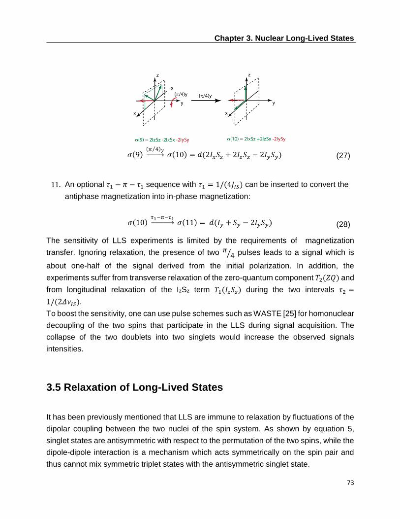
Chapter 3. Nuclear Long-Lived States
73
𝜎(9)
(𝜋 4⁄ )𝑦→ 𝜎(10) = 𝑑(2𝐼𝑥𝑆𝑧 + 2𝐼𝑧𝑆𝑥 − 2𝐼𝑦𝑆𝑦) (27)
11. An optional 𝜏1 − 𝜋 − 𝜏1 sequence with 𝜏1 = 1/(4𝐽𝐼𝑆) can be inserted to convert the
antiphase magnetization into in-phase magnetization:
𝜎(10) 𝜏1−𝜋−𝜏1→ 𝜎(11) = 𝑑(𝐼𝑦 + 𝑆𝑦 − 2𝐼𝑦𝑆𝑦) (28)
The sensitivity of LLS experiments is limited by the requirements of magnetization
transfer. Ignoring relaxation, the presence of two 𝜋 4⁄ pulses leads to a signal which is
about one-half of the signal derived from the initial polarization. In addition, the
experiments suffer from transverse relaxation of the zero-quantum component 𝑇2(𝑍𝑄) and
from longitudinal relaxation of the IzSz term 𝑇1(𝐼𝑧𝑆𝑧) during the two intervals 𝜏2 =
1/(2𝛥𝜈𝐼𝑆).
To boost the sensitivity, one can use pulse schemes such as WASTE [25] for homonuclear
decoupling of the two spins that participate in the LLS during signal acquisition. The
collapse of the two doublets into two singlets would increase the observed signals
intensities.
3.5 Relaxation of Long-Lived States
It has been previously mentioned that LLS are immune to relaxation by fluctuations of the
dipolar coupling between the two nuclei of the spin system. As shown by equation 5,
singlet states are antisymmetric with respect to the permutation of the two spins, while the
dipole-dipole interaction is a mechanism which acts symmetrically on the spin pair and
thus cannot mix symmetric triplet states with the antisymmetric singlet state.

3.5 Relaxation of Long-Lived States
74
In its simplest form, relaxation can be described by Bloch's equations, which provide a
phenomenological picture of relaxation. Bloch’s formulation does not provide any
microscopic explanation of the origin of relaxation, nor does it allow to predict the
magnitude of the rate constants. This limitation can be overcome by treating relaxation
quantum mechanically.
In Liouville space, the relaxation rates of populations and coherences can be obtained as
eigenvalues of the matrix representation of the relaxation superoperator in an appropriate
operator basis. The set of basis operators is chosen as the one containing all
eigenoperators 𝑄𝑟 obtained by commutation with the total spin angular momentum along
the z-axis 𝐼𝑧:
𝐼𝑧𝑄𝑟 = 𝑝𝑟𝑄𝑟 (29)
where the integer value 𝑝𝑟 is called the coherence order.
If a superoperator 𝑨 commutes with the superoperator Iz, the matrix representation of 𝑨 is
block-diagonal in the chosen basis set 𝑏 with a block for each possible value of the
coherence order 𝑝 [21]:
The matrix block containing operators with the same coherence order p will be denoted
as [𝑨]𝑝𝑏. In the context of singlet states relaxation, it is convenient to use an operator basis
where the basis operators are built from an appropriate combination of all the 16 products
of the type [10]:
|𝑠⟩⟨𝑟| (30)
where |𝑠⟩ ∈ {|𝑆0⟩, |𝑇−1⟩, |𝑇0⟩, |𝑇+1⟩}
⟨𝑟| ∈ {⟨𝑆0|, ⟨𝑇−1|,⟨𝑇0|, ⟨𝑇+1| }

Chapter 3. Nuclear Long-Lived States
75
Furthermore, it is sufficient to consider only the zero-quantum block of the relaxation
matrix to examine the relaxation properties of LLS because the singlet state belongs to
this block and is not coupled to any blocks with different coherence orders.[21]
Figure 4 Redfield kite structure of the relaxation supermatrix [26].
The zero-quantum block (𝑝 = 0) of the operator basis is:
𝑆𝑇𝐵0 =
{
1
2(|𝑆0⟩⟨𝑆0| + |𝑇+1⟩⟨𝑇+1| + |𝑇0⟩⟨𝑇0| + |𝑇−1⟩⟨𝑇−1|)
1
2√3(3|𝑆0⟩⟨𝑆0| − |𝑇+1⟩⟨𝑇+1| − |𝑇0⟩⟨𝑇0| − |𝑇−1⟩⟨𝑇−1| )
1
√2(|𝑇+1⟩⟨𝑇+1| − |𝑇−1⟩⟨𝑇−1|)
1
√6(2|𝑇0⟩⟨𝑇0| − |𝑇+1⟩⟨𝑇+1| − |𝑇−1⟩⟨𝑇−1| )
|𝑆0⟩⟨𝑇0|
|𝑇0⟩⟨𝑆0| }
(31)
The first operator in this zero-quantum block (𝑄1𝑆𝑇𝐵0) is one-half of the unity operator and
commutes with all other spin operators. The second basis operator (𝑄2𝑆𝑇𝐵0) has an
expectation value proportional to the deviation of the singlet population from a uniform
population distribution. The third (𝑄3𝑆𝑇𝐵0) and the fourth (𝑄4
𝑆𝑇𝐵0) operators represent
perturbations of the triplet populations, the third one having an expectation value

3.5 Relaxation of Long-Lived States
76
proportional to the total longitudinal magnetization for the two nuclei. Finally, the last two
operators (𝑄5𝑆𝑇𝐵0) and (𝑄6
𝑆𝑇𝐵0) represent zero-quantum singlet-triplet coherences.
3.5.1 The homogeneous master equation
The dynamics of a spin system can be described by the homogeneous Liouville-von
Neumann master equation:
𝑑
𝑑𝑡𝜎(𝑡) = −𝐿(𝑡)𝜎(𝑡) (32)
where 𝜎(𝑡) is the density matrix representation and 𝐿 the Liouvillian superoperator, which
represents a superposition of both coherent and incoherent effects on the spin-system,
described respectively by the commutation superoperators 𝐻0 and Γ:
𝐿(𝑡) = −𝑖𝐻0(𝑡)+ Γ (33)
In a frame rotating at a frequency 𝜔𝑅𝐹 (preferably corresponding to the average of the
chemical shifts of the two spins), the coherent superoperator can be written as [27]
𝐻0 = 𝜔𝐼𝐼𝑧 +𝜔𝑆𝐼𝑧 + 2𝜋𝐽𝐼𝑆 + 𝜔𝑛𝑢𝑡(𝐼𝑥 + 𝑆𝑥) (34)
where 𝜔𝐼 and 𝜔𝑆 are the offsets of the two spins 𝐼 and 𝑆, respectively, and 𝜔𝑛𝑢𝑡 is the
amplitude of the CW RF field with frequency 𝜔𝑅𝐹 applied to suppress the chemical shift
difference of the two spins, making them equivalent in the sense of average Hamiltonian
theory.
The superoperator 𝐿 contains a superposition of the contributions of all possible relaxation
mechanisms:
Γ = Γ𝐷𝐷 + Γ𝐶𝑆𝐴 + Γ𝑆𝑅 + Γ𝑃𝑆 + ∑ Γ𝑗𝑘𝑗,𝑘 (35)

Chapter 3. Nuclear Long-Lived States
77
where Γ𝐷𝐷 is the contribution due to the dipole-dipole (DD) interaction between the two
spins, Γ𝐶𝑆𝐴 is the contribution of the chemical shift anisotropy, Γ𝑆𝑅 is the contribution of the
spin rotation mechanism and Γ𝑃𝑆 is the contribution of interactions with the paramagnetic
species, while ∑ Γ𝑗𝑘𝑗,𝑘 is the sum of all cross-correlation terms, such as DD-CSA, etc..
From now on it is necessary to distinguish the types of mechanisms that cause relaxation.
In the following paragraph, the attention will be focused on the dipolar mechanism
between the spin pair, in order to demonstrate its inefficiency for the relaxation of LLS.
3.5.2 The dipolar relaxation mechanism
As mentioned, it is possible to demonstrate, by symmetry arguments, that the singlet state
of two spin-1/2 nuclei is immune to the DD relaxation mechanism.
Singlet states are anti-symmetric with respect to spin exchange, while the dipole-dipole
interaction acts symmetrically on the two coupled nuclei and thus cannot mix symmetric
and anti-symmetric states. Therefore, singlet and triplet states are never interchanged.
A theoretical explanation requires examination of the zero-quantum block of the matrix
representation of Γ𝐼𝑆𝐷𝐷 in the 𝑆𝑇𝐵0 basis [21] :
[Γ𝐼𝑆𝐷𝐷]0
𝑆𝑇𝐵0 = −𝑏𝐼𝑆2 𝜏𝑐10
(
0 0 0 0 0 00 0 0 0 0 00 0 15 0 0 00 0 0 9 0 00 0 0 0 5 00 0 0 0 0 5)
(36)
where 𝑏𝐼𝑆 = −(ℏ𝜇0𝛾𝐼𝛾𝑆)/(4𝜋𝑟𝐼𝑆3 ) is the dipolar coupling constant.
The zero-quantum block is diagonal and 𝑄2𝑆𝑇𝐵0 is, indeed, an eigenoperator of the
superoperator DD
IS . Its eigenvalue corresponds therefore to the decay rate of the singlet
population. At the same time, the longitudinal magnetization −𝑄2𝑆𝑇𝐵0 has a non-vanishing
decay rate. Hence in the extreme narrowing regime [21]:
𝑅𝑠𝐷𝐷 = 0 (37)

3.5.2 The dipolar relaxation mechanism
78
𝑅1𝐷𝐷 =
3
2𝑏𝐼𝑆2 𝜏𝑐 (38)
The relaxation rate of the singlet state 𝑅𝑠𝐷𝐷 due to the dipolar interaction between the spin
pair vanishes. The singlet state population is immune to this kind of interaction. On the
other hand,
the correspondent longitudinal magnetization decay rate 𝑅1𝐷𝐷 does not vanish
and is consistent with that derived by Redfield relaxation theory.
As a result, if a population imbalance between singlet and triplet states is excited, the main
relaxation mechanism in solution is switched off. Relaxation of this long-lived state will
occur due to secondary mechanisms, like dipolar couplings with “out-of-pair” nuclear spins
or paramagnetic species, chemical shift anisotropy, spin rotation, and so on.

Chapter 3. Nuclear Long-Lived States
79
References
1. M. Carravetta and M. H. Levitt, Theory of long-lived nuclear spin states in solution
nuclear magnetic resonance. I. Singlet states in low magnetic field. Journal of
Chemical Physics, 2005. 122(21): p. 14.
2. G. Pileio, M. Carravetta, E. Hughes, and M. H. Levitt, The long-lived nuclear singlet
state of N-15-nitrous oxide in solution. Journal of the American Chemical Society,
2008. 130(38): p. 12582-+.
3. R. Sarkar, P. Ahuia, D. Moskau, P. R. Vasos, and G. Bodenhausen, Extending the
scope of singlet-state spectroscopy. Chemphyschem, 2007. 8(18): p. 2652-2656.
4. R. Sarkar, P. R. Vasos, and G. Bodenhausen, Singlet-state exchange NMR
spectroscopy for the study of very slow dynamic processes. Journal of the
American Chemical Society, 2007. 129(2): p. 328-334.
5. E. Y. Chekmenev, J. Hovener, V. A. Norton, K. Harris, L. S. Batchelder, P.
Bhattacharya, B. D. Ross, and D. P. Weitekamp, PASADENA hyperpolarization of
succinic acid for MRI and NMR spectroscopy. Journal of the American Chemical
Society, 2008. 130(13): p. 4212-4213.
6. T. C. Eisenschmid, R. U. Kirss, P. P. Deutsch, S. I. Hommeltoft, R. Eisenberg, J.
Bargon, R. G. Lawler, and A. L. Balch, Para Hydrogen Induced Polarization in
Hydrogenation Reactions. Journal of the American Chemical Society, 1987.
109(26): p. 8089-8091.
7. A. Bornet, X. Ji, D. Mammoli, B. Vuichoud, J. Milani, G. Bodenhausen, and S.
Jannin, Long-Lived States of Magnetically Equivalent Spins Populated by
Dissolution-DNP and Revealed by Enzymatic Reactions. Chemistry-a European
Journal, 2014. 20(51): p. 17113-17118.
8. D. Mammoli, B. Vuichoud, A. Bornet, J. Milani, J. N. Dumez, S. Jannin, and G.
Bodenhausen, Hyperpolarized para-Ethanol. Journal of Physical Chemistry B,
2015. 119(10): p. 4048-4052.
9. G. Pileio, M. Carravetta, and M. H. Levitt, Storage of nuclear magnetization as long-
lived singlet order in low magnetic field. Proceedings of the National Academy of
Sciences of the United States of America, 2010. 107(40): p. 17135-17139.
10. G. Pileio and M. H. Levitt, Theory of long-lived nuclear spin states in solution
nuclear magnetic resonance. II. Singlet spin locking. Journal of Chemical Physics,
2009. 130(21).

References
80
11. J. H. Ardenkjaer-Larsen, B. Fridlund, A. Gram, G. Hansson, L. Hansson, M. H.
Lerche, R. Servin, M. Thaning, and K. Golman, Increase in signal-to-noise ratio of
> 10,000 times in liquid-state NMR. Proceedings of the National Academy of
Sciences of the United States of America, 2003. 100(18): p. 10158-10163.
12. M. C. D. Tayler, I. Marco-Rius, M. I. Kettunen, K. M. Brindle, M. H. Levitt, and G.
Pileio, Direct Enhancement of Nuclear Singlet Order by Dynamic Nuclear
Polarization. Journal of the American Chemical Society, 2012. 134(18): p. 7668-
7671.
13. P. R. Vasos, A. Comment, R. Sarkar, P. Ahuja, S. Jannin, J. P. Ansermet, J. A.
Konter, P. Hautle, B. van den Brandt, and G. Bodenhausen, Long-lived states to
sustain hyperpolarized magnetization. Proceedings of the National Academy of
Sciences of the United States of America, 2009. 106(44): p. 18469-18473.
14. P. Ahuja, R. Sarkar, S. Jannin, P. R. Vasos, and G. Bodenhausen, Proton
hyperpolarisation preserved in long-lived states. Chemical Communications, 2010.
46(43): p. 8192-8194.
15. C. Laustsen, G. Pileio, M. C. D. Tayler, L. J. Brown, R. C. D. Brown, M. H. Levitt,
and J. H. Ardenkjaer-Larsen, Hyperpolarized singlet NMR on a small animal
imaging system. Magnetic Resonance in Medicine, 2012. 68(4): p. 1262-1265.
16. R. Sarkar, P. Ahuja, P. R. Vasos, and G. Bodenhausen, Measurement of Slow
Diffusion Coefficients of Molecules with Arbitrary Scalar Couplings via Long-Lived
Spin States. Chemphyschem, 2008. 9(16): p. 2414-2419.
17. P. Ahuja, R. Sarkar, P. R. Vasos, and G. Bodenhausen, Diffusion Coefficients of
Biomolecules Using Long-Lived Spin States. Journal of the American Chemical
Society, 2009. 131(22): p. 7498-+.
18. Aurelien Bornet, Puneet Ahuja, Riddhiman Sarkar, Laetitia Fernandes, Sonia Hadji,
Shirley Y. Lee, Aydin Haririnia, David Fushman, Geoffrey Bodenhausen, and Paul
R. Vasos, Long-Lived States to Monitor Protein Unfolding by Proton NMR.
Chemphyschem, 2011. 12(15): p. 2729-2734.
19. M. Carravetta, O. G. Johannessen, and M. H. Levitt, Beyond the T-1 limit: Singlet
nuclear spin states in low magnetic fields. Physical Review Letters, 2004. 92(15).
20. M. Carravetta and M. H. Levitt, Long-lived nuclear spin states in high-field solution
NMR. Journal of the American Chemical Society, 2004. 126(20): p. 6228-6229.
21. Giuseppe Pileio, Relaxation theory of nuclear singlet states in two spin-1/2
systems. Progress in Nuclear Magnetic Resonance Spectroscopy, 2010. 56(3): p.
217-231.

Chapter 3. Nuclear Long-Lived States
81
22. G. Bodenhausen and K. Gopalakrishnan, Lifetimes of the singlet-states under
coherent off-resonance irradiation in NMR spectroscopy. Journal of Magnetic
Resonance, 2006. 182(2): p. 254-259.
23. J. Keeler, Understanding NMR Spectroscopy, ed. Wiley. 2005.
24. P. J. Hore, J. A. Jones, and S. Wimperis, NMR: The Toolkit, ed. O.S. Publication.
2000.
25. D. Carnevale, T. F. Segawa, and G. Bodenhausen, Polychromatic Decoupling of a
Manifold of Homonuclear Scalar Interactions in Solution-State NMR. Chemistry-a
European Journal, 2012. 18(37): p. 11573-11576.
26. Bodenhausen G. Ernst R. R., Wokaun A., ed. Principles of Nuclear Magnetic
Resonance in One and Two Dimensions. 1990, Oxford University Press.
27. M.H. Levitt, ed. Spin dynamics. 2008, Wiley: Chichester.

82

Chapter 4. The use of Long-Lived States for studying ligand-protein interactions
83
4. The use of Long-Lived States for studying ligand-protein
interactions
he first step of drug discovery is commonly referred to as hit identification.
Screening techniques such as enzyme-linked immunosorbent assays (ELISA),[1]
surface plasmon resonance (SPR, also known under the trade name Biacore),[2]
isothermal titration calorimetry (ITC),[3] and an ever-expanding range of nuclear magnetic
resonance (NMR) techniques [4-6] allow one to recognize ligands for a defined protein
contained in extensive libraries of chemical compounds.
Because one can choose from a wide range of observable parameters, NMR
spectroscopy offers several methods to study interactions between small ligand molecules
and macromolecular targets. It is possible to extract dissociation constants [7] and to
obtain structural information about the protein and its complex with the ligand.[8] Provided
the exchange between the free and bound forms of the ligand is faster than the difference
of their resonance frequencies,[8, 9] i.e., when 𝑘𝑒𝑥 ≈ 𝑘𝑜𝑓𝑓 ≫ (𝜋/√2)Δ𝜐, where Δ𝜐 is the
chemical shift difference (in Hz) of the signals in the bound and free states, any observable
quantity 휀𝑜𝑏𝑠, be it a frequency or a relaxation rate, is determined by a weighted average
of the free and bound forms [10]:
휀𝑜𝑏𝑠 = 𝑝𝐵휀𝐵 + 𝑝𝐹휀𝐹 (1)
where 𝑝𝐵 and 𝑝𝐹 are the mole fractions of the bound and free ligands, respectively, while
휀𝐵 and 휀𝐹 are the values of the parameter 휀 in the bound and free forms, respectively.
Observation of differences between 휀𝑜𝑏𝑠 and 휀𝐹 allows the detection of ligand binding.
Provided that 휀𝐵 ≠ 휀𝐹, differences between 휀𝑜𝑏𝑠 and 휀𝐹 can be detected if there is a certain
amount of ligand in the bound form, i.e., 𝑝𝐵 > 0.
The sensitivity of a parameter 휀 to binding events can be expressed by the experimental
contrast 𝐶𝜀, which is a function of the “observable” parameters 휀𝑜𝑏𝑠 and 휀𝐹:
𝐶𝜀 = |𝜀𝑜𝑏𝑠− 𝜀𝐹
𝜀𝑜𝑏𝑠| ∗ 100 (2)
The larger the contrast, the more sensitive the parameter 휀 to ligand–protein binding, i.e.,
smaller the fraction of ligand in the bound form 𝑝𝐵 that is required to detect binding.
T

4. The use of Long-Lived States for studying ligand-protein interactions
84
Several NMR methods based on such a contrast are extensively used nowadays to
determine dissociation constants of ligand–protein interactions. The quantity 휀𝑜𝑏𝑠 can be
determined by the chemical shifts of one or more selected nuclei of either target proteins
[11] or ligands,[12] the translational or rotational diffusion constant of the ligand,[13] the
relaxation rates 𝑇1, 𝑇2 or 𝑇1𝜌, the rate of magnetization transfer by cross-relaxation
(Overhauser effect) between protons belonging to the ligand,[14] the saturation transfer
from proteins to ligands determined by difference spectroscopy,[15] or “waterLOGSY” that
exploits differences in the rate of transfer of magnetization from bulk water to free or bound
ligands by cross-relaxation.[16] Several of these methods rely on differences in rotational
correlation times between the free ligand and the protein–ligand complex.[17]
It has been recently demonstrated that so-called Long-Lived States (LLS), also known as
singlet states (SS) in isolated two-spin systems, can be used very efficiently to investigate
protein-ligand interactions.[18] In the following paragraphs, the use of LLS for this purpose
will be described and experimental results will be discussed.
4.1 LLS contrast
s mentioned in the previous paragraph, detection of ligand-receptor binding is
obtained through observation of a difference between 휀𝑜𝑏𝑠 and 휀𝐹. Equation 1
nicely shows that such a difference is possible only if 휀𝐵 ≠ 휀𝐹. In particular, the
larger the difference between 휀𝐵 and 휀𝐹, the smaller the fraction of ligand in the bound
form 𝑝𝐵 required to generate a sufficient difference between the parameters 휀𝑜𝑏𝑠 and 휀𝐹.
In other words, for a fixed ligand-to-receptor ratio [𝐿]/[𝑃], i.e., a fixed 𝑝𝐵, large differences
between 휀𝐵 and 휀𝐹 lead to a large experimental contrast 𝐶𝜀, while small differences
between 휀𝐵 and 휀𝐹 lead to a small value of 𝐶𝜀. Combining equation 1 with the definitions
𝑝𝐵 = [𝑃𝐿]/[𝐿]𝑡𝑜𝑡 and 𝑝𝐹 = ([𝐿]𝑡𝑜𝑡 − [𝑃𝐿])/[𝐿]𝑡𝑜𝑡, one gets:
휀𝑜𝑏𝑠 = [𝑃𝐿]
[𝐿]𝑡𝑜𝑡(휀𝐵 − 휀𝐹) + 휀𝐹 (3)
Equation 3 can be used to fit the variation of an observed parameter during a titration in
order to extrapolate the dissociation constant 𝐾𝐷, since the ratio [𝑃𝐿] [𝐿]𝑡𝑜𝑡⁄ is a function
of 𝐾𝐷. It we rearrange equation 3, we obtain:
A

Chapter 4. The use of Long-Lived States for studying ligand-protein interactions
85
(휀𝑜𝑏𝑠 − 휀𝐹) = [𝑃𝐿]
[𝐿]𝑡𝑜𝑡(휀𝐵 − 휀𝐹) (4)
Equation 4 correlates directly the experimental difference (휀𝑜𝑏𝑠 − 휀𝐹) with the difference
(휀𝐵 − 휀𝐹) between the values of the parameter 휀 in the bound and free forms, showing
that the larger the difference (휀𝐵 − 휀𝐹), the smaller the bound fraction 𝑝𝐵 = [𝑃𝐿]/[𝐿]𝑡𝑜𝑡
required to obtain a detectable (휀𝑜𝑏𝑠 − 휀𝐹).
The LLS relaxation rate 𝑅𝐿𝐿𝑆 is extremely sensitive to ligand-protein binding. Long-lived
states have the unique property that their populations relax with time constants that can
be much longer than longitudinal relaxation time constants (𝑇𝐿𝐿𝑆 ≫ 𝑇1). The intensity 𝐼 of
the LLS signal decays mono-exponentially as a function of the sustaining delay 𝜏𝑚:
𝐼(𝜏𝑚) = 𝐼0exp (−𝑅𝐿𝐿𝑆𝜏𝑚) (5)
where 𝐼0 is the LLS intensity at 𝜏𝑚 = 0 and 𝑅𝐿𝐿𝑆 is the LLS relaxation rate. The LLS
relaxation rate 𝑅𝐿𝐿𝑆 and thus the LLS lifetime 𝑇𝐿𝐿𝑆 = 1/𝑅𝐿𝐿𝑆 can be extracted by fitting the
signal intensity observed as a function of the sustaining delay 𝜏𝑚. For pairs of protons,
𝑇𝐿𝐿𝑆/𝑇1 ratios as large as 60 have been observed in R-CH=CH-R’ systems.
Glycine residues in peptides contain two diastereotopic Hα protons, so it is straightforward
to excite LLS in virtually any glycine-containing peptide.[19] It has been shown by phage
display [20] using a peptide library and consensus sequence analysis that peptides that
bind to Urokinase-type Plasminogen Activator (uPA) must contain at least one arginine
residue.[21] We therefore considered the GGR tripeptide, which turns out to be a weak
binder for uPA.
The two Hα protons of the central glycine residue are not magnetically equivalent, due to
the vicinity of the chiral Cα carbon of the arginine residue. Hence, it is possible to excite
long-lived states with the pulse sequence described in chapter 3.[22] The lifetime 𝑇𝐿𝐿𝑆 of
this pair of diastereotopic Hα protons was determined to be 𝑇𝐿𝐿𝑆 = (8.0 ± 0.2) 𝑠 at 8 ºC
and 9.4 T.[18] Under the same conditions, the longitudinal relaxation time 𝑇1 turned out to
be 𝑇1 = (0.40 ± 0.08) 𝑠, leading to a ratio 𝑇𝐿𝐿𝑆/𝑇1 as large as 20.

4.1 LLS contrast
86
Figure 1 Chemical structure of the tripeptide GGR. The two Hα protons of the central glycine residue are highlighted in red. The chiral Cα carbon of the arginine residue is indicated by a star.
The situation changes drastically if there are interactions between ligands and proteins.
We simulated the dipole-dipole contributions (the main relaxation pathways in solution-
state NMR spectroscopy if chemical shift anisotropy can be neglected) to the 𝑅1 and 𝑅𝐿𝐿𝑆
relaxation rates of the free and bound tripeptide GGR. For the conventional longitudinal
relaxation rates 𝑅1, the dipole-dipole interactions between the protons of the ligand and
those lining the binding site of uPA contribute roughly to 85% of the observed contrast.
Moreover, the structures of free GGR and of the GGR-uPA complex in water were
optimized using Gromacs 4.5.3 [23] using the GROMOS 53a6 force field.[24] The
chemical shifts of the free and bound ligands were calculated by using these structures
as input for Camshift 1.35.[25] The chemical shifts of the two Hα protons of the central
glycine residue in GGR in the free and bound forms were estimated by modeling to change
by ca. 0.5 ppm (200 Hz at 9.4 T in our experiments). Conventional longitudinal relaxation
is not influenced by such a shift, but it has a dramatic effect on the lifetimes of the LLS.[26,
27] Indeed, during the LLS relaxation period, a radiofrequency (RF) field must be used to
mask the chemical shift difference between the two Hα protons involved in the LLS. This
field is most efficient when the carrier frequency coincides precisely with the center
between the shifts of the two Hα protons, as we chose for the free ligand. When the ligand
is bound, there is a frequency mismatch due to the change in chemical shifts upon binding,
and the LLS decays rapidly, so that its lifetime is reduced. Indeed, figure 2 shows that ca.
75% of the decay rate of the LLS signal is due to the coherent effect of the frequency
mismatch that occurs upon binding. This effect can be enhanced by using weaker RF
fields or higher static fields.

Chapter 4. The use of Long-Lived States for studying ligand-protein interactions
87
Figure 2 (Top) The tripeptide glycine-glycine-arginine (GGR) and its complex with Urokinase-type Plasminogen Activator (uPA). (Middle) Frequency jumps of the two Hα protons of the central glycine of GGR when it forms a complex with uPA. It is estimated that the two chemical shifts of the Hα protons jump by 0.5 ppm (200 Hz at 9.4 T) as the ligand goes from the free (green solid line) to the bound forms (red dashed line). The spectrum of the bound ligand cannot be observed directly because of fast exchange. The chemical shifts are weighted averages of the values in the free and bound forms. (Bottom) Relative contributions to the decay rate 𝑅𝐿𝐿𝑆 = 1/𝑇𝐿𝐿𝑆 of the long-lived state of the two Hα protons in the complex. The RF field used
to sustain the LLS was monochromatic with an amplitude of 𝜈1 = 1 𝑘𝐻𝑧, well above the minimum required
to mask the chemical shift difference 𝛿(𝐻𝛼) − 𝛿(𝐻𝛼′) = 100 𝐻𝑧 in the free ligand.
The combination of a slow relaxation rate 𝑅𝐿𝐿𝑆𝑓𝑟𝑒𝑒
< 𝑅1𝑓𝑟𝑒𝑒
of the ligand in its free state with
a rapid relaxation rate 𝑅𝐿𝐿𝑆𝑏𝑜𝑢𝑛𝑑 in its bound state makes the difference (𝑅𝐿𝐿𝑆
𝑏𝑜𝑢𝑛𝑑 − 𝑅𝐿𝐿𝑆𝑓𝑟𝑒𝑒
)
particularly large, thus making the relaxation of long-lived state an extremely sensitive
NMR parameter to ligand-protein binding.
To demonstrate the enhancement of the contrast 𝐶𝐿𝐿𝑆 with respect to the contrast 𝐶1 and
𝐶1𝜌, binding experiments were carried out for a 1 mM solution of the tripeptide ligand GGR
in the presence of its protein target trypsin in the range 0.5 < [𝑃] < 50 µM, using various
methods (𝑇𝐿𝐿𝑆, 𝑇1 and 𝑇1𝜌). Figure 3 shows that the LLS method can work with a protein-
ligand ratio that is ~25-fold lower that required for the well-known 𝑇1𝜌 method, whereas

4.1 LLS contrast
88
the 𝑇1 contrast remains below 𝐶1 < 10 % even at the highest protein concentration [𝑃] =
50 µM.
Figure 3 Experimental contrast for 𝑇𝐿𝐿𝑆 (red), 𝑇1𝜌 (green), and 𝑇1 (blue) methods for the diastereotopic pair
of protons on the central glycine residue of the tripeptide GGR in a solution with a fixed concentration [𝐿] =1 mM and a variable trypsin concentration 0.5 µM < [𝑃]0 < 50 µM in D2O at 8 ºC and 11.7 T.
4.2 Competition experiments
quation 3 can be used to fit the variation of the observed LLS relaxation rate 𝑅𝐿𝐿𝑆𝑜𝑏𝑠
during the titration of a ligand against a target:
𝑅𝐿𝐿𝑆𝑜𝑏𝑠 =
[𝑃𝐿]
[𝐿]𝑡𝑜𝑡(𝑅𝐿𝐿𝑆
𝑏𝑜𝑢𝑛𝑑 − 𝑅𝐿𝐿𝑆𝑓𝑟𝑒𝑒
) + 𝑅𝐿𝐿𝑆𝑓𝑟𝑒𝑒
(6)
The fitting allows one to estimate the LLS relaxation rate of the bound form 𝑅𝐿𝐿𝑆𝑏𝑜𝑢𝑛𝑑 and
the molar fraction of the ligand in the bound form 𝑝𝐵 = [𝑃𝐿] [𝐿]𝑡𝑜𝑡⁄ . The latter parameter
is a function of the dissociation constant 𝐾𝐷 [28]:
[𝑃𝐿]
[𝐿]𝑡𝑜𝑡=
[𝑃]𝑡𝑜𝑡+[𝐿]𝑡𝑜𝑡+𝐾𝐷−√([𝑃]𝑡𝑜𝑡+[𝐿]𝑡𝑜𝑡+𝐾𝐷)2−4[𝑃]𝑡𝑜𝑡[𝐿]𝑡𝑜𝑡
2[𝐿]𝑡𝑜𝑡
(7)
E

Chapter 4. The use of Long-Lived States for studying ligand-protein interactions
89
As consequence, it is possible to determine the dissociation constant by fitting the
variation of the observed relaxation rate during a titration experiment. For example, the
ligand GGR was titrated over a range 0.5 mM < [𝐿]𝑡𝑜𝑡 < 10 mM in the presence of [𝑃]𝑡𝑜𝑡 =
10 µM uPA at 8 ºC. The curve in figure 4 was fitted to equation 6, yielding 𝐾𝐷 = 220 ± 10
µM and 𝑇𝐿𝐿𝑆𝑏𝑜𝑢𝑛𝑑 = 1/𝑅𝐿𝐿𝑆
𝑏𝑜𝑢𝑛𝑑 = 30 ± 10 ms. In contrast, as shown in figure 4, binding had
virtually no effect on the longitudinal relaxation rates 𝑅1 = 1/𝑇1 of the same Hα protons.
Figure 4 Lifetimes 𝑇𝐿𝐿𝑆 of the long-lived state associated with the two Hα protons of the central glycine residue of the weak ligand L = GGR and their conventional longitudinal relaxation times 𝑇1 in the presence
of [𝑃]𝑡𝑜𝑡= 10 µM uPA as a function of [𝐿]𝑡𝑜𝑡 at 8 ºC and 400 MHz in D2O. The curve shows a fit of the
experimental data to equation 6.
Experiments based on the direct observation of ligands suffer from some limitations: non-
specific binders may give similar effects as specific ones, ligands are difficult to detect if
their solubility is low, and strong ligands in slow exchange are easily mistaken for non-
binders. Indeed, when binding is too strong, the lifetime of the ligand-protein complex may
be too long on the NMR time scale, so that the conditions for equation 1 are not fulfilled
and the rates are not properly averaged.
To overcome these drawbacks, Dalvit and co-workers [29] introduced competition
experiments for ligand screening. In this approach, a weak-affinity ligand is used as a spy
molecule; a stronger binder partly displaces the spy molecule, and the latter’s expulsion
from the binding site of the macromolecular target leads to a decrease of relaxation rates
of nuclei that belong to the displaced spy ligand. Of course, the contrast defined above
should be sufficient. The concentration of the competitor that is required to displace the
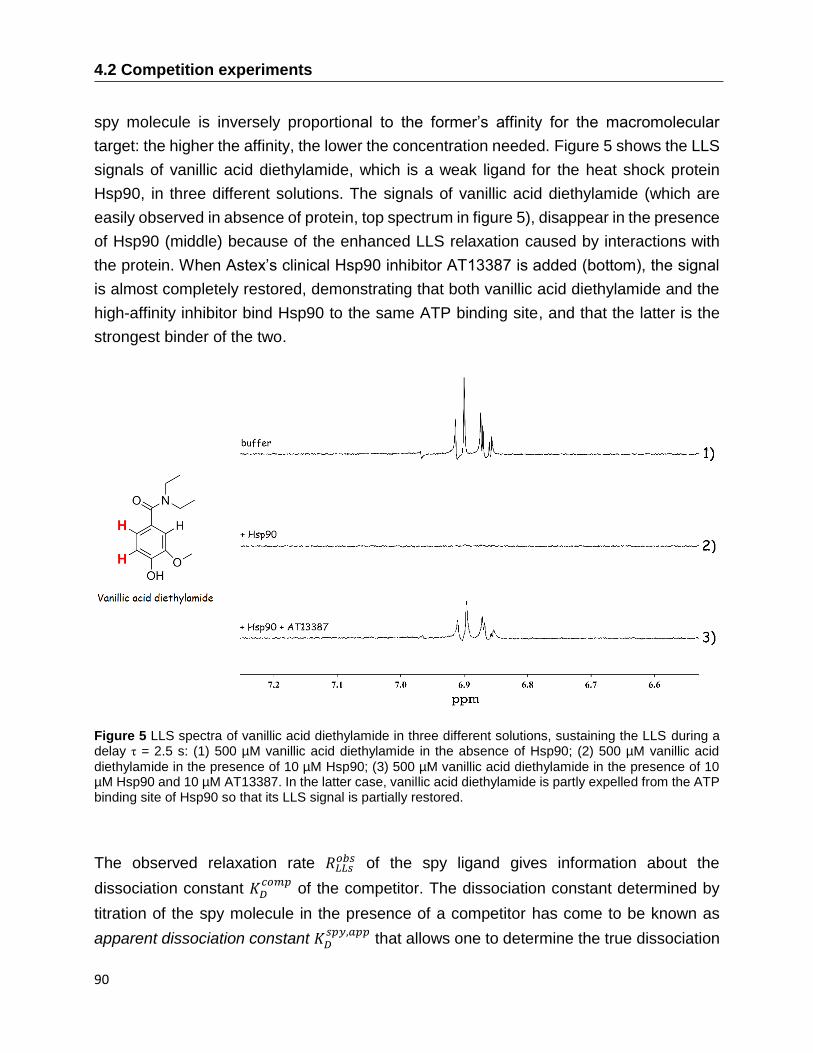
4.2 Competition experiments
90
spy molecule is inversely proportional to the former’s affinity for the macromolecular
target: the higher the affinity, the lower the concentration needed. Figure 5 shows the LLS
signals of vanillic acid diethylamide, which is a weak ligand for the heat shock protein
Hsp90, in three different solutions. The signals of vanillic acid diethylamide (which are
easily observed in absence of protein, top spectrum in figure 5), disappear in the presence
of Hsp90 (middle) because of the enhanced LLS relaxation caused by interactions with
the protein. When Astex’s clinical Hsp90 inhibitor AT13387 is added (bottom), the signal
is almost completely restored, demonstrating that both vanillic acid diethylamide and the
high-affinity inhibitor bind Hsp90 to the same ATP binding site, and that the latter is the
strongest binder of the two.
Figure 5 LLS spectra of vanillic acid diethylamide in three different solutions, sustaining the LLS during a delay τ = 2.5 s: (1) 500 µM vanillic acid diethylamide in the absence of Hsp90; (2) 500 µM vanillic acid
diethylamide in the presence of 10 µM Hsp90; (3) 500 µM vanillic acid diethylamide in the presence of 10 µM Hsp90 and 10 µM AT13387. In the latter case, vanillic acid diethylamide is partly expelled from the ATP binding site of Hsp90 so that its LLS signal is partially restored.
The observed relaxation rate 𝑅𝐿𝐿𝑠𝑜𝑏𝑠 of the spy ligand gives information about the
dissociation constant 𝐾𝐷𝑐𝑜𝑚𝑝
of the competitor. The dissociation constant determined by
titration of the spy molecule in the presence of a competitor has come to be known as
apparent dissociation constant 𝐾𝐷𝑠𝑝𝑦,𝑎𝑝𝑝
that allows one to determine the true dissociation

Chapter 4. The use of Long-Lived States for studying ligand-protein interactions
91
constant 𝐾𝐷𝑐𝑜𝑚𝑝
of the competitor. The relationship between these two constants is
expressed by the following equation:
𝐾𝐷
𝑐𝑜𝑚𝑝 = [𝐿𝑐𝑜𝑚𝑝]𝑡𝑜𝑡 𝐾𝐷
𝑠𝑝𝑦
𝐾𝐷𝑠𝑝𝑦,𝑎𝑝𝑝
− 𝐾𝐷𝑠𝑝𝑦
(8)
where [𝐿𝑐𝑜𝑚𝑝]𝑡𝑜𝑡 is the concentration of the competitor and 𝐾𝐷𝑠𝑝𝑦
is the true dissociation
constant of the spy molecule.
Note that the competitor does not need to contain any spin pairs that can sustain an LLS.
Moreover, by keeping the concentration of the spy ligand low, one can study competing
ligands with limited solubility. Furthermore, as the changes in 𝑅𝐿𝐿𝑠𝑜𝑏𝑠 need only to be
observed for the spy molecule, there are no requirements for the competitor to fulfill the
fast-exchange condition. This implies that the dissociation constants 𝐾𝐷𝑐𝑜𝑚𝑝
of the
competitor can lie anywhere in a wide range below 100 µM. Following this approach, GGR
was used as spy molecule and titrated over a range 0.5 mM < [𝐿𝑠𝑝𝑦]𝑡𝑜𝑡 < 10 mM in the
presence of [𝑃]𝑡𝑜𝑡 = 10 µM uPA and [𝐿𝑐𝑜𝑚𝑝]𝑡𝑜𝑡 = 10 µM of two different competitors at 8
ºC. In this fashion, 𝐾𝐷𝑐𝑜𝑚𝑝
= 89 ± 20 µM was determined for 4-aminobenzamidine, which
has a better affinity than GGR but is not strong enough to inhibit uPA. Next, the bicyclic
peptide ligand UK-18 has been investigated. This ligand has a high affinity and specificity
for uPA [30], and indeed 𝐾𝐷𝑐𝑜𝑚𝑝
= 180 ± 20 nM was determined by the LLS method [18],
in good agreement with previously published results obtained by Heinis and co-workers
(𝐾𝐷𝑐𝑜𝑚𝑝
= 157 ± 39 nM) [30] and Stubbs and co-workers (𝐾𝐷𝑐𝑜𝑚𝑝
= 180 nM).[31]
4.3 Spin-pair labeling for ligand LLS experiments
drawback of ligand screening by LLS is that the ligands (or only the spy ligand in
the competition approach) must carry a pair of nonequivalent spins with I = 1/2.
When such ligands are not immediately available in the compound libraries,
synthetic labeling strategies can circumvent this issue. These approaches include two
steps: 1) the identification of a spy ligand that binds weakly to the target protein, and 2)
the functionalization of this ligand by attaching a spin-pair label that can carry LLS. By
way of illustration, 3-bromothiophene-2-carboxylic acid (henceforth called “BT”), which is
known to have long lifetimes 𝑇𝐿𝐿𝑆 [32], has been covalently attached to the tripeptide GGR.
A

4.3 Spin-pair labeling for ligand LLS experiments
92
The resulting spin-pair-labeled tripeptide was called BT-GGR (figure 6b). It is a weak
ligand for trypsin. [33]
Despite some steric effects and long-range dipolar relaxation mechanisms in the spin-
pair-labeled tripeptide BT-GGR, the two aromatic protons of the bromothiophene group
retain a remarkably long lifetime 𝑇𝐿𝐿𝑆(BT) = 11.7 ± 0.7 s in the absence of protein. In this
particular tripeptide, both diastereotopic pairs of Hα protons on the two glycine residues of
BT-G1G2R can be used to excite LLS. They have lifetimes 𝑇𝐿𝐿𝑆(G1) = 10.4 ± 0.5 s and
𝑇𝐿𝐿𝑆(G2) = 9.3 ± 0.5 s again in the absence of protein.
The spin-pair-labeled ligand BT-GGR was added to a solution containing [𝑃]𝑡𝑜𝑡 = 25 µM
trypsin over a range 0.5 mM < [𝐿]𝑡𝑜𝑡 < 40 mM. At each concentration, the observed
relaxation times 𝑇𝐿𝐿𝑆𝑜𝑏𝑠 = 1/𝑅𝐿𝐿𝑆
𝑜𝑏𝑠 of the three different pairs of protons were measured.
Figure 6a shows how the titration curves can be fitted to equation 6. As expected, nearly
the same dissociation constants were obtained for the three proton pairs that can sustain
LLS in BT-GGR: 𝐾𝐷(BT) = 0.18 ± 0.03 mM, 𝐾𝐷(G1) = 0.24 ± 0.01 mM, and 𝐾𝐷(G2) = 0.21
± 0.02 mM.
Figure 6 LLS titration experiments. a) Observed LLS lifetimes of the three proton pairs on the spin-pair-
labeled tripeptide BT-GGR as a function of the ligand concentration [𝐿]𝑡𝑜𝑡, in the presence of 25 µM trypsin in D2O at 25 ºC and 11.7 T. b) Pairs of protons capable of sustaining LLS in BT-GGR: on bromothiophene BT (red), on the N-terminal glycine G1 (blue) and on the central glycine G2 (green).

Chapter 4. The use of Long-Lived States for studying ligand-protein interactions
93
The functionalized ligand can be used as spy molecule in competition experiments, once
the dissociation constant 𝐾𝐷𝑠𝑝𝑦
of the spin-pair labeled spy ligand and its LLS lifetime in
the bound form 𝑇𝐿𝐿𝑆𝑏𝑜𝑢𝑛𝑑 are known. It is possible to optimize the competitor [𝐿𝑐𝑜𝑚𝑝]𝑡𝑜𝑡 and
protein [𝑃]𝑡𝑜𝑡 concentrations to rank strong competitors according to their binding
strengths. Figure 7 shows the calculated 𝑇𝐿𝐿𝑆𝑜𝑏𝑠 (BT) of the bromothiophene protons in BT-
GGR if [𝑃]𝑡𝑜𝑡 = 25 µM and [𝐿𝑐𝑜𝑚𝑝]𝑡𝑜𝑡 = 50 µM as a function of the dissociation constant
𝐾𝐷𝑐𝑜𝑚𝑝
of the competitor. Under these conditions, 𝑇𝐿𝐿𝑆𝑜𝑏𝑠 changes dramatically in the range
between 𝐾𝐷𝑐𝑜𝑚𝑝
= 100 µM and 𝐾𝐷𝑐𝑜𝑚𝑝
= 1 µM.
Figure 7 Effect of a competitor on the lifetime 𝑇𝐿𝐿𝑆𝑜𝑏𝑠 of a spy molecule. The lifetime of the pair of aromatic
protons of bromothiophene (BT) depends on the dissociation constant of the competing ligand, calculated using equations 6, 7 and 8. The parameters of the spy molecule BT-GGR were obtained from the fit of the
data in figure 6: 𝐾𝐷 = 0.2 mM, 𝑇𝐿𝐿𝑆𝑏𝑜𝑢𝑛𝑑 = 0.1 s, 𝑇𝐿𝐿𝑆
𝑓𝑟𝑒𝑒 = 11 s, [𝐿𝑠𝑝𝑦]𝑡𝑜𝑡 = 0.5 mM, [𝑃]𝑡𝑜𝑡 = 25 µM, and [𝐿𝑐𝑜𝑚𝑝]𝑡𝑜𝑡
= 50 µM. The three points correspond to 𝑇𝐿𝐿𝑆𝑜𝑏𝑠 in the presence of myricetin (𝐾𝐷
𝑐𝑜𝑚𝑝 = 3 µM, green), apigenin
(𝐾𝐷𝑐𝑜𝑚𝑝
= 39 µM, blue) and in the absence of any competitor (red) calculated for these conditions.
A library of competing ligands can thus be ranked according to their affinities by observing
the LLS signal of a spy ligand. Under the conditions shown in figure 7, one can easily rank
competing ligands with great accuracy, provided 1 µM < 𝐾𝐷𝑐𝑜𝑚𝑝
< 100 µM. The ranking of
ligands can be achieved by performing LLS experiments with a single sustaining delay
𝜏𝑚. As the observed relaxation rate 𝑅𝐿𝐿𝑆𝑜𝑏𝑠 of the spy ligand is attenuated in the presence of
a stronger competitor, the LLS signal intensity of the spy ligand after a suitably chosen
delay 𝜏𝑚 will be enhanced. For instance, LLS spectra of 0.5 mM BT-GGR were recorded
with 𝜏𝑚 = 3 s in the presence of [𝑃]𝑡𝑜𝑡 = 25 µM trypsin with four different competitors, all
with [𝐿𝑐𝑜𝑚𝑝]𝑡𝑜𝑡 = 50 µM: myricetin (𝐾𝐷𝑐𝑜𝑚𝑝
= 3 µM), morin (𝐾𝐷𝑐𝑜𝑚𝑝
= 30 µM), apigenin (𝐾𝐷𝑐𝑜𝑚𝑝

4.3 Spin-pair labeling for ligand LLS experiments
94
= 39 µM) [34] and benzamydine (𝐾𝐷𝑐𝑜𝑚𝑝
= 39 µM).[31] Figure 8a shows three of the five
LLS spectra, obtained either without competitor (red), with apigenin (blue), or with
myricetin (green). Figure 8b shows the signal intensities of the spy ligand BT-GGR in the
presence of one of the four competing ligands.
Note that the spin-lock duration m has to be chosen carefully to tune the experiment to
the expected range of affinities. Equation 8 can be used to estimate the apparent
dissociation constant of the spy molecule 𝐾𝐷𝑠𝑝𝑦,𝑎𝑝𝑝
, and equations 7 and 6 then allow one
to estimate the relaxation rate RLLS of the spy molecule in the presence of a competitor.
Once this relaxation rate is known, the spin-lock duration can be set to maximize the
difference between the signals of the spy molecule with and without competitor.
Figure 8 LLS competition binding experiments. a) Signals of one of the two aromatic protons of bromothiophene (BT) in the spy ligand BT-GGR at a concentration of 0.5 mM in the presence of 25 µM trypsin, sustaining the LLS for 𝜏𝑚 = 3 s in D2O at 25 ºC and 11.7 T: 1) in the absence of any competitor (red), 2) in competition with 50 µM of the intermediate ligand apigenin (blue), and 3) in competition with 50 µM of the stronger ligand myricetin (green). b) Peak intensities of one of the aromatic protons of BT-GGR under the same conditions as in a), without competitor and in the presence of apigenin, benzamidine, morin,
or myricetin. The better the binding, the smaller the dissociation constant 𝐾𝐷𝑐𝑜𝑚𝑝
, the more effective the
displacement of the spin-pair-labeled spy ligand BT-GGR, and the more intense its LLS signal.

Chapter 4. The use of Long-Lived States for studying ligand-protein interactions
95
4.4 Hyperpolarized LLS ligand screening experiments
t is obviously desirable to use low concentrations of both proteins and ligands, not only
to save expensive materials, but also to avoid protein and ligand aggregation and to
be able to study poorly soluble ligands. The ligand concentrations cannot be very low
because of the intrinsic poor sensitivity of NMR. At ligand concentrations [𝐿]𝑡𝑜𝑡 < 100 µM,
NMR spectra require extensive signal averaging to show sufficient signal-to-noise ratios
(SNR).
Hyperpolarization of nuclear spins by dissolution dynamic nuclear polarization (D-DNP)
[35] can overcome this problem. By microwave irradiation of samples containing radicals
at temperatures close to 𝑇 = 1.2 K, the polarization of electron spins can be transferred to
protons or other nuclei, followed by rapid dissolution of the hyperpolarized samples and
their transfer to a high-resolution NMR spectrometer for detection. Enhancements 휀𝐷𝑁𝑃
up to five orders of magnitude can be obtained for nuclei with low gyromagnetic ratios,
while enhancements 100 < 휀𝐷𝑁𝑃 < 1000 can be achieved for 1H or 19F nuclei.[36] The
technique has not been very popular for 1H and 19F nuclei so far, because rapid 𝑇1
relaxation tends to cause losses of polarization during the transfer from the polarizer to
the spectrometer.
Ligands with covalently attached spin-pair labels such as BT-GGR contain protons with
long 𝑇1 values and are therefore suitable for hyperpolarization by dissolution DNP. Indeed,
provided 𝑇1(1H) > 1 s, a sufficient fraction of the hyperpolarized magnetization can be
preserved during the transfer from the DNP polarizer to the NMR spectrometer.
In our laboratory, BT-GGR has been hyperpolarized by DNP and used as a spy ligand in
LLS competition binding experiments.[33] We shall give a brief protocol for these
experiments. In a glass-forming solvent mixture H2O/D2O/DMSO-d6 (v/v/v = 5:35:60), 10
mM BT-GGR are dissolved with 25 mM 4-hydroxy-2,2,6,6-tetramethylpiperidine-1-oxyl
(TEMPOL). Five frozen beads (5 x 10 µL) of this solution are loaded together with five
frozen beads (5 x 10 µL) of 3 M ascorbate [37] into a home-built DNP polarizer [38, 39]
operating at 𝐵0 = 6.7 T and 𝑇 = 1.2 K. The sample is irradiated with microwaves at a
frequency 𝑓𝑚𝑊 = 188.3 GHz and power 𝑃𝑚𝑊 = 100 mW. At 𝐵0 = 6.7 T, a proton polarization
up to 𝑃(1H) = 90 % can be obtained [39], while 𝑃(1H) is only ~ 40 % in polarizers operating
at 𝐵0 = 3.35 T. After ~ 15 min of microwave irradiation, a steady-state proton 𝑃(1H) can
generally be reached.
The DNP sample can be dissolved rapidly in 0.7 s with 5 mL of hot D2O (𝑃 = 1 MPa, 𝑇 =
400 K) and transferred to a 11.7 T NMR spectrometer in 4.5 s through a “magnetic tunnel”
I
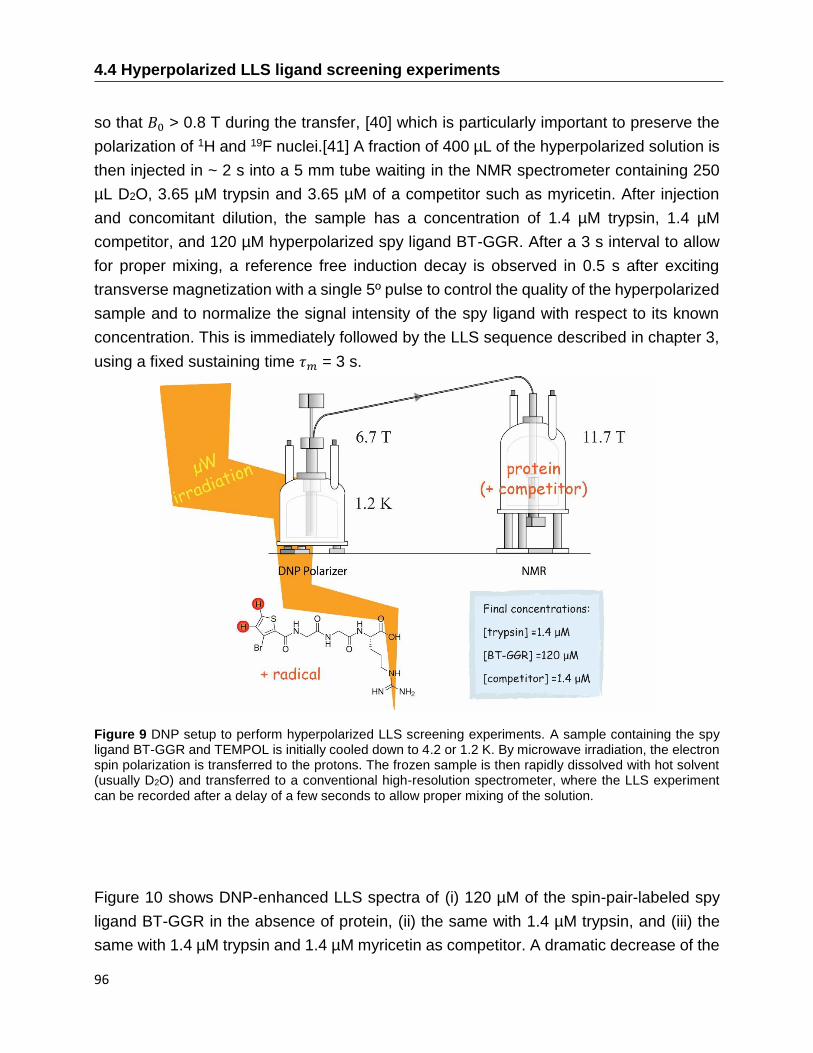
4.4 Hyperpolarized LLS ligand screening experiments
96
so that 𝐵0 > 0.8 T during the transfer, [40] which is particularly important to preserve the
polarization of 1H and 19F nuclei.[41] A fraction of 400 µL of the hyperpolarized solution is
then injected in ~ 2 s into a 5 mm tube waiting in the NMR spectrometer containing 250
µL D2O, 3.65 µM trypsin and 3.65 µM of a competitor such as myricetin. After injection
and concomitant dilution, the sample has a concentration of 1.4 µM trypsin, 1.4 µM
competitor, and 120 µM hyperpolarized spy ligand BT-GGR. After a 3 s interval to allow
for proper mixing, a reference free induction decay is observed in 0.5 s after exciting
transverse magnetization with a single 5º pulse to control the quality of the hyperpolarized
sample and to normalize the signal intensity of the spy ligand with respect to its known
concentration. This is immediately followed by the LLS sequence described in chapter 3,
using a fixed sustaining time 𝜏𝑚 = 3 s.
Figure 9 DNP setup to perform hyperpolarized LLS screening experiments. A sample containing the spy ligand BT-GGR and TEMPOL is initially cooled down to 4.2 or 1.2 K. By microwave irradiation, the electron spin polarization is transferred to the protons. The frozen sample is then rapidly dissolved with hot solvent (usually D2O) and transferred to a conventional high-resolution spectrometer, where the LLS experiment can be recorded after a delay of a few seconds to allow proper mixing of the solution.
Figure 10 shows DNP-enhanced LLS spectra of (i) 120 µM of the spin-pair-labeled spy
ligand BT-GGR in the absence of protein, (ii) the same with 1.4 µM trypsin, and (iii) the
same with 1.4 µM trypsin and 1.4 µM myricetin as competitor. A dramatic decrease of the

Chapter 4. The use of Long-Lived States for studying ligand-protein interactions
97
LLS signal intensity stemming from BT-GGR is observed in the presence of trypsin. An
equimolar amount of the competitor myricetin leads to a partial displacement of the spy
ligand that can be readily detected through the revival of its LLS signal. With only 120 µM
of BT-GGR, the DNP-enhanced LLS spectrum of figure 10 recorded in a single scan after
𝜏𝑚 = 3 s has a signal-to-noise ratio of 130. Under the same conditions, but without DNP,
an accumulation of 225 transients for ~1 h was necessary to reach the same SNR.
Figure 10 DNP-enhanced LLS competition binding experiments. DNP-enhanced LLS spectra of the two
aromatic protons of bromothiophene in 120 µM BT-GGR after a sustaining time τm = 3 s, (i) without protein
(black), (ii) in the presence of 1.4 µM trypsin (orange), (iii) with 1.4 µM trypsin and 1.4 µM myricetin as
competitor (green). All spectra were acquired in a single scan in D2O at 25 ºC and 11.7 T.
A DNP-enhanced LLS spectrum of BT-GGR with a concentration as low as 10 µM could
be recorded with a SNR of 16. Clearly, DNP allows one to decrease the concentration of
ligands, but the protein concentration should not be decreased further. Indeed, lower
protein concentrations would diminish the observed contrast. Figure 11 shows the protein
concentration [𝑃]𝑡𝑜𝑡 necessary to obtain a satisfactory contrast 𝐶𝐿𝐿𝑆 = 50 %, depending
on the ligand concentration, for different dissociation constants. If 𝐾𝐷 = 200 µM, a protein
with cannot be diluted to nanomolar concentrations without sacrificing contrast. It is clear
that when [𝐿]𝑡𝑜𝑡 < 𝐾𝐷, it is does not make sense to decrease the protein concentration
further, since this leads to a loss of contrast 𝐶𝐿𝐿𝑆.
Without DNP, using a 50-fold increase in ligand concentration (figure 8), 256 transients
had to be accumulated in 100 min to obtain a SNR of 8. The experimental conditions can
be adapted depending on the primary objective: low concentrations of either protein or
ligand, rapid throughput, high sensitivity for the displacement by a competitor, or high
SNR. In figure 10, the conditions were optimized for high SNR and high contrast upon

4.4 Hyperpolarized LLS ligand screening experiments
98
addition of a competitor, albeit at the expense of a slightly higher ligand concentration and
longer polarization build-up time. To attain faster throughput, one could polarize at a
higher temperature 𝑇 = 4.2 K and 𝐵0 = 6.7 T, where proton polarization 𝑃(1H) = 25 % can
be reached by DNP in ~ 2 min.[39] The price to pay would be an approximate three-fold
lower SNR. Similarly, at 𝑇 = 1.2 K and 𝐵0 = 3.35 T, as in commercially available DNP
polarizers, 𝑃(1H) = 40 % can be reached in ~ 6 min.[32]
Figure 11 Protein concentrations required to obtain a 50 % LLS contrast for different ligand concentrations.
When [𝐿]𝑡𝑜𝑡 < 𝐾𝐷, the required protein concentration to obtain a sufficient contrast approaches a plateau. The decrease of the protein concentration below the plateau leads to a drop of contrast. These simulations are based on equations 6 and 7.
With the set-up used to perform these experiments, the time required for the transfer from
the polarizer to the detection magnet is similar to 𝑇1(1H) of the spy ligand BT-GGR. A
significant fraction of the proton hyperpolarization is lost during the 10 s interval between
dissolution and signal acquisition. Nevertheless, a faster sample injection device [41]
could decrease this interval to 1.2 s. An acceleration of the transfer would enhance the
remaining proton polarization and thus the SNR. Such improvements would allow either
a further decrease in ligand concentration or an increase in sample throughput.
After dissolution, the sample temperature could not be monitored in our experiments.
Nevertheless, one can assume that during the “voyage” through the magnetic tunnel, the
hyperpolarized solution reaches room temperature. In any case, potential temperature

Chapter 4. The use of Long-Lived States for studying ligand-protein interactions
99
drifts of the final solution after dissolution should not affect the ranking of competitors,
since the temperature should affect the restoration of the signals of the spy molecule in a
uniform and reproducible manner.
4.5 Exploring weak ligand-protein interactions by LLS
n fragment-based drug discovery (FBDD), fragment screening is performed using
relatively small libraries of carefully chosen compounds with low molecular weights
(120-250 Da). Useful fragments typically have dissociation constants 𝐾𝐷 ranging from
0.1 to 10 mM or greater. Techniques that can detect ligand-protein complexes, such as
X-ray crystallography, surface plasmon resonance (SPR), isothermal titration calorimetry
(ITC), and high-concentration assays can be used for fragment screening. The output of
these target-based methods depends on the fraction of bound protein with respect to the
total protein concentration.[42] If the binding affinities are weak, the equilibrium can only
be shifted by increasing the concentration of the fragments, which must therefore be highly
soluble, a requirement that is difficult to meet.
In ligand-based methods the output is given by the fraction 𝑝𝐵 = [𝑃𝐿]/[𝐿]𝑡𝑜𝑡 of bound
ligands with respect to the total ligand concentration.[42] So despite its low intrinsic
sensitivity, the detection of ligands by NMR spectroscopy can be used over an extremely
wide dynamic range of dissociation constants 𝐾𝐷 while requiring only relatively low protein
and ligand concentrations. In contrast to the above-mentioned biophysical techniques,
NMR allows one to perform screening with ligand concentrations [𝐿]𝑡𝑜𝑡 that are orders of
magnitude lower than the corresponding dissociation constants 𝐾𝐷.
As has been shown in chapter 2, the fraction 𝑝𝐵 of ligand in the bound form depends on
the affinity of the ligand. In particular, for a given ligand [𝐿]𝑡𝑜𝑡 and protein concentration
[𝑃]𝑡𝑜𝑡, the larger the dissociation constant, the lower the fraction of ligand in the bound
form 𝑝𝐵 (see figure 2, chapter 2). As consequence, the detection of weak interactions
turns out to be challenging.
Equation 4 shows that, for a fixed value of 𝑝𝐵, the ability of detecting the binding event
depends on the difference (휀𝐵 − 휀𝐹) between the values of the parameter 휀 in the free and
bound forms. In the case of long-lived states, the difference Δ𝑅𝐿𝐿𝑆 = (𝑅𝐿𝐿𝑆𝑏𝑜𝑢𝑛𝑑 − 𝑅𝐿𝐿𝑆
𝑓𝑟𝑒𝑒) can
be much larger than Δ𝑅1, Δ𝑅2, etc., so that it is possible to achieve a high contrast 𝐶𝐿𝐿𝑆
even for high ligand/protein ratios, making LLS-based screening particularly attractive for
a fragment-based approach that seeks to identify weakly binding ligands.
I

4.5 Exploring weak ligand-protein interactions by LLS
100
Figure 12 shows mole fractions 𝑝𝐵 of bound ligands for different ligand/protein ratios and
the corresponding contrast 𝐶𝐿𝐿𝑆 during a titration of vanillic acid diethylamide against the
N-terminal ATPase domain of heat shock protein 90 (Hsp90). Long-lived states were
excited on the two aromatic protons of the ligand. Even for a large ligand-to-protein ratio
[𝐿]𝑡𝑜𝑡 [𝑃]𝑡𝑜𝑡⁄ = 272, one observes a dramatic 45 % contrast.
A contrast 𝐶𝐿𝐿𝑆 = 23 %, corresponding to a ratio 𝑅𝑜𝑏𝑠/𝑅𝑓𝑟𝑒𝑒 = 1.3, can be achieved with a
ratio [𝐿]𝑡𝑜𝑡/[𝑃]𝑡𝑜𝑡 = 707, i.e., under conditions where less than 0.2 % of the ligand is bound
to the protein. Compared to other 1H-detected NMR methods, which suffer from lower
contrast, this allows ligand binding to be detected for low protein concentrations and/or
low binding affinities. One can thus more easily customize the concentrations of proteins
and ligands to study very weak affinities in screening assays. For example, to detect
ligands with 𝐾𝐷 ≤ 1 mM and [L] = 500 µM, one would require a protein concentration [P] =
3 µM; alternatively, if [P] = 20 µM one can detect binding even if 𝐾𝐷 > 10 mM. Such weak
affinities are typically encountered for fragments that bind to protein-protein interfaces.
This offers considerable advantages over fragment screening by traditional ligand-based
NMR methods.
Figure 12 (Left) Structure of vanillic acid diethylamide. The pair of aromatic protons that is suitable for the excitation of LLS is indicated by bold red letters. (Right) Molar fractions of bound ligands for different ligand/protein ratios and the experimentally observed contrast 𝐶𝐿𝐿𝑆 for a titration of vanillic acid diethylamide
(𝐾𝐷 = 790 µM) in the presence of the protein Hsp90.
LLS screening is most effectively carried out in competition mode, as proposed by Dalvit
et al. [29] for traditional 𝑅1 and 𝑅2 experiments: a strongly binding ligand partly displaces
a weakly binding ‘spy’ ligand from the binding site, so that one observes a decrease of the
relaxation rate 𝑅𝐿𝐿𝑆 of the displaced spy ligand.

Chapter 4. The use of Long-Lived States for studying ligand-protein interactions
101
Obviously, the search for weak binders by a competition approach is a difficult task, since
the spy ligand has to be displaced by a weaker competitor. Nevertheless, it has been
demonstrated that LLS can efficiently reach this goal. Vanillic acid diethylamide (𝐾𝐷 = 790
µM) has been used as spy ligand in LLS competition screening experiments against
Hsp90.[43] The performance of LLS screening in competition mode with a mixture
containing known binders and known non-binders has been tested. Indeed, if a library of,
say, 1000 compounds is to be screened against a protein target, it is most efficient to
screen ‘cocktails’ containing typically 3-10 ligands, to reduce experimental time and
protein consumption. In the absence of competing binders, the interaction between the
spy ligand and the protein leads to rapid LLS relaxation and hence to the attenuation of
the LLS signal (spectrum 1 in Figure 13); conversely, the presence of a competitor leads
to a partial displacement of the spy ligand, hence to slower LLS relaxation and a partial
restoration of the LLS signal of the spy (spectrum 2 in Figure 13). This change in LLS
signal is due to a mere 13 % change in the amount of bound ligand, which itself is only
0.3 % of the total ligand concentration.
Once the presence of a binder in a mixture has been demonstrated, a deconvolution step
is needed to identify the hit, as shown in Figure 13 (spectrum 3), which allowed the
identification of 3-hydroxyindazole as a weak binder for Hsp90.
Note that to displace a weak spy ligand by fragments that are binding even more weakly,
the latter must be present at similar concentrations. This is a considerable advantage over
other NMR methods used in competition mode, which because of lower contrast require
much higher concentrations to achieve effective displacements, as they require small
ligand/protein ratios to detect weak ligands. Furthermore, if the mixtures comprise many
components, the NMR resonances of the spy molecule may be obscured by overlapping
signals [44], which may hamper all NMR methods when used in competition mode.
Fortunately, the LLS sequence in effect eliminates signals that do not stem from long-lived
states. As shown by spectrum 2 in Figure 13, resonances that arise from other compounds
are considerably reduced, compared to the conventional 1H spectrum of the same mixture
(spectrum 4).
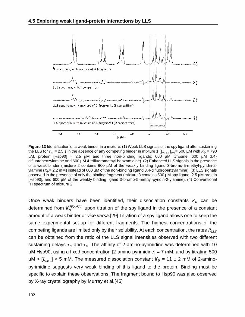
4.5 Exploring weak ligand-protein interactions by LLS
102
Figure 13 Identification of a weak binder in a mixture. (1) Weak LLS signals of the spy ligand after sustaining the LLS for 𝜏𝑚 = 2.5 s in the absence of any competing binder in mixture 1 ([𝐿𝑠𝑝𝑦]𝑡𝑜𝑡= 500 µM with 𝐾𝐷 = 790
µM, protein [Hsp90] = 2.5 µM and three non-binding ligands: 600 µM tyrosine, 600 µM 3,4-difluorobenzylamine and 600 µM 4-trifluoromethyl-benzamidine). (2) Enhanced LLS signals in the presence of a weak binder (mixture 2 contains 600 µM of the weakly binding ligand 3-bromo-5-methyl-pyridin-2-ylamine (𝐾𝐷= 2.2 mM) instead of 600 µM of the non-binding ligand 3,4-difluorobenzylamine). (3) LLS signals observed in the presence of only the binding fragment (mixture 3 contains 500 µM spy ligand, 2.5 µM protein [Hsp90], and 600 µM of the weakly binding ligand 3-bromo-5-methyl-pyridin-2-ylamine). (4) Conventional 1H spectrum of mixture 2.
Once weak binders have been identified, their dissociation constants 𝐾𝐷 can be
determined from 𝐾𝐷𝑠𝑝𝑦,𝑎𝑝𝑝
upon titration of the spy ligand in the presence of a constant
amount of a weak binder or vice versa.[29] Titration of a spy ligand allows one to keep the
same experimental set-up for different fragments. The highest concentrations of the
competing ligands are limited only by their solubility. At each concentration, the rates 𝑅𝐿𝐿𝑆
can be obtained from the ratio of the LLS signal intensities observed with two different
sustaining delays 𝜏𝑎 and 𝜏𝑏. The affinity of 2-amino-pyrimidine was determined with 10
μM Hsp90, using a fixed concentration [2-amino-pyrimidine] = 7 mM, and by titrating 500
μM < [𝐿𝑠𝑝𝑦] < 5 mM. The measured dissociation constant 𝐾𝐷 = 11 ± 2 mM of 2-amino-
pyrimidine suggests very weak binding of this ligand to the protein. Binding must be
specific to explain these observations. The fragment bound to Hsp90 was also observed
by X-ray crystallography by Murray et al.[45]

Chapter 4. The use of Long-Lived States for studying ligand-protein interactions
103
Figure 14 (Grey line) Direct titration of the spy ligand vanillic acid diethylamide in the presence of 10 μM Hsp90 protein. (Black line) Competition experiment with titration of vanillic acid diethylamide as a spy ligand in the presence of 10 μM Hsp90 protein and a constant concentration of 7 mM of 2-amino-pyrimidine.
Note that the choice of the spy molecule determines the experimental conditions of the
LLS assay. With a spy molecule such as vanillic acid diethylamide (𝐾𝐷𝑠𝑝𝑦
= 790 µM), a
concentration of 7 mM of the competing 2-amino-pyrimidine (𝐾𝐷 = 12 mM) gives rise to
19% contrast (first point of black curve in Figure 14). This can be reduced to 3.3 mM to
give rise to a 10% contrast, which is sufficient to show binding in screening experiments,
as shown in Figure 13 for 3-hydroxyindazole (difference between spectra 1 and 2). If the
expected affinities of fragments for a particular target are on the order of 𝐾𝐷 = 5 mM or
higher, it is most convenient to identify and use a weaker spy molecule that would ensure
a 10% contrast while working at lower fragment concentrations. As a consequence, one
can effectively screen and identify weak fragments with very low solubility.
The ability of measuring accurate binding constants in the mM range, where methods
such ITC and high concentration assays may fail, in particular when the ligand solubility
is limited, enables the investigation of structure-activity relationships and the guidance of
initial steps of hit optimization chemistry.

4.6 Extending LLS ligand screening to 19F nuclei
104
4.6 Extending LLS ligand screening to 19F nuclei
n competition experiments, the concentration of the competitor that is required to
displace the spy molecule is inversely proportional to the former’s affinity for the
macromolecular target: the higher the affinity, the lower the concentration needed. The
study of weakly binding fragments turns out to be challenging since high concentrations
and thus high solubility are required. Moreover, if mixtures of competitors are tested, the
risk of signal overlap must be circumvented by a careful choice of the cocktail of
molecules.
The excitation of LLS involving pairs of 19F nuclei belonging to spy ligands that have been
designed to feature a favorable contrast CLLS between free and bound forms allows one
to study weak protein-ligand interactions while avoiding signal overlap. 19F detection offers
several advantages [46] over 1H detection: a) high sensitivity, since 19F has a high
gyromagnetic ratio and 100% natural abundance; b) absence of overlap with protonated
solvents, buffers or detergents; c) absence of overlap with other molecules if experiments
are performed on chemical mixtures with many components; d) high sensitivity of
transverse 𝑅2 relaxation of 19F to binding, as seen in chapter 2.
Long-lived states have so far only been observed in systems comprising 1H, 13C or 15N
nuclei.[47] We have synthetized a molecule that contains a pair of diastereotopic aliphatic
fluorine atoms: 1,1-difluoro-1-phenylacetyl-Gly-Arg, abbreviated as DFPA-GR (figure 15).
The presence of an arginine residue assures a weak binding affinity for the active site of
trypsin [21], thus allowing one to explore the behavior of LLS of pairs of 19F nuclei upon
binding. Aliphatic fluorine atoms have been preferred to aromatic ones, in order to
minimize LLS relaxation due to CSA contributions. In fact, amino acids with 19F-labels in
aliphatic positions have shown smaller CSA values than in aromatic compounds with 19F
substituents on the ring. [48, 49] [48, 49] [48, 49]
Figure 15 Structure of DFPA-GR that contains a pair of aliphatic diastereotopic fluorine atoms (red), which are magnetically inequivalent because of the vicinity of a chiral center (*).
I
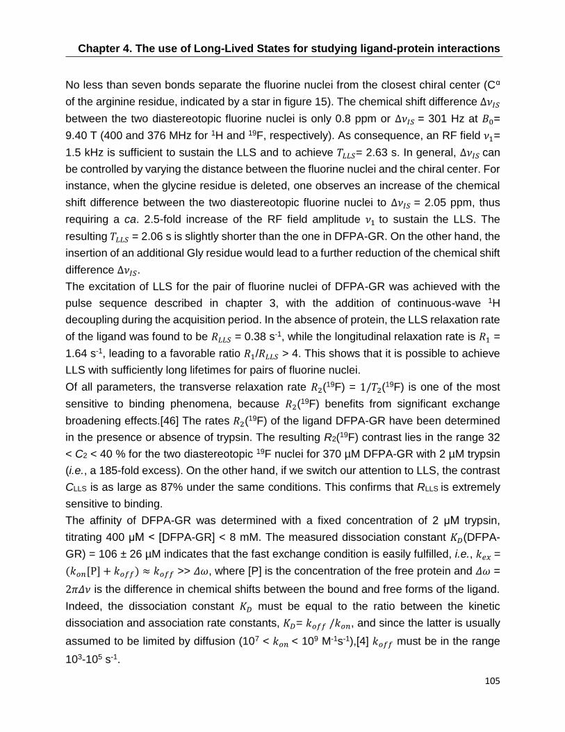
Chapter 4. The use of Long-Lived States for studying ligand-protein interactions
105
No less than seven bonds separate the fluorine nuclei from the closest chiral center (Cα
of the arginine residue, indicated by a star in figure 15). The chemical shift difference Δ𝜈𝐼𝑆
between the two diastereotopic fluorine nuclei is only 0.8 ppm or Δ𝜈𝐼𝑆 = 301 Hz at 𝐵0=
9.40 T (400 and 376 MHz for 1H and 19F, respectively). As consequence, an RF field 𝜈1=
1.5 kHz is sufficient to sustain the LLS and to achieve 𝑇𝐿𝐿𝑆= 2.63 s. In general, Δ𝜈𝐼𝑆 can
be controlled by varying the distance between the fluorine nuclei and the chiral center. For
instance, when the glycine residue is deleted, one observes an increase of the chemical
shift difference between the two diastereotopic fluorine nuclei to Δ𝜈𝐼𝑆 = 2.05 ppm, thus
requiring a ca. 2.5-fold increase of the RF field amplitude 𝜈1 to sustain the LLS. The
resulting 𝑇𝐿𝐿𝑆 = 2.06 s is slightly shorter than the one in DFPA-GR. On the other hand, the
insertion of an additional Gly residue would lead to a further reduction of the chemical shift
difference Δ𝜈𝐼𝑆.
The excitation of LLS for the pair of fluorine nuclei of DFPA-GR was achieved with the
pulse sequence described in chapter 3, with the addition of continuous-wave 1H
decoupling during the acquisition period. In the absence of protein, the LLS relaxation rate
of the ligand was found to be 𝑅𝐿𝐿𝑆 = 0.38 s-1, while the longitudinal relaxation rate is 𝑅1 =
1.64 s-1, leading to a favorable ratio 𝑅1/𝑅𝐿𝐿𝑆 > 4. This shows that it is possible to achieve
LLS with sufficiently long lifetimes for pairs of fluorine nuclei.
Of all parameters, the transverse relaxation rate 𝑅2(19F) = 1/𝑇2(19F) is one of the most
sensitive to binding phenomena, because 𝑅2(19F) benefits from significant exchange
broadening effects.[46] The rates 𝑅2(19F) of the ligand DFPA-GR have been determined
in the presence or absence of trypsin. The resulting R2(19F) contrast lies in the range 32
< C2 < 40 % for the two diastereotopic 19F nuclei for 370 µM DFPA-GR with 2 µM trypsin
(i.e., a 185-fold excess). On the other hand, if we switch our attention to LLS, the contrast
CLLS is as large as 87% under the same conditions. This confirms that RLLS is extremely
sensitive to binding.
The affinity of DFPA-GR was determined with a fixed concentration of 2 μM trypsin,
titrating 400 μM < [DFPA-GR] < 8 mM. The measured dissociation constant 𝐾𝐷(DFPA-
GR) = 106 ± 26 µM indicates that the fast exchange condition is easily fulfilled, i.e., 𝑘𝑒𝑥 =
(𝑘𝑜𝑛[P] + 𝑘𝑜𝑓𝑓) ≈ 𝑘𝑜𝑓𝑓 >> 𝛥𝜔, where [P] is the concentration of the free protein and 𝛥𝜔 =
2𝜋𝛥𝜈 is the difference in chemical shifts between the bound and free forms of the ligand.
Indeed, the dissociation constant 𝐾𝐷 must be equal to the ratio between the kinetic
dissociation and association rate constants, 𝐾𝐷= 𝑘𝑜𝑓𝑓 /𝑘𝑜𝑛, and since the latter is usually
assumed to be limited by diffusion (107 < 𝑘𝑜𝑛 < 109 M-1s-1),[4] 𝑘𝑜𝑓𝑓 must be in the range
103-105 s-1.

4.6 Extending LLS ligand screening to 19F nuclei
106
Figure 16 (Top) Signals derived from 19F-19F LLS of 500 µM DPFA-GR in the absence of trypsin after 𝜏𝑚 = 0.7 s. (Center) the same in the presence of 2 µM trypsin. (Bottom) in the presence of 2 µM trypsin and 485 µM morin as competitor, which partly displaces DPFA-GR from the binding site of the protein, leading to a partial restoration of its signals. A total of 128 scans were recorded for each spectrum, with acquisition and repetition times of 0.7 and 3 s, respectively.
Once a suitable spy ligand such as DFPA-GR that fulfills the fast exchange regime has
been identified, libraries of potential binders can be screened by competition experiments
[29] by observing changes in the LLS decay rates of the spy ligand. Figure 16 shows the
LLS spectrum of 500 µM DFPA-GR in the absence of protein (top), in the presence of 2
µM trypsin (center) and with 2 µM trypsin plus 485 µM morin, a well-known trypsin inhibitor
[50] (bottom). Since a competitor like morin partly displaces the spy molecule from the
binding site of the protein, its presence leads to a partial restoration of the LLS signals of
the spy ligand.
Once a competitor has been identified, its dissociation constant needs to be determined.
To do so, the spy DFPA-GR can be titrated in the presence of a constant concentration of
competitor or vice versa [29]. The curve of TLLS vs. [𝐿𝑠𝑝𝑦] can be fitted using equation 6 to
extrapolate an apparent dissociation constant 𝐾𝐷𝑠𝑝𝑦,𝑎𝑝𝑝
. The dissociation constant 𝐾𝐷𝑐𝑜𝑚𝑝
of the competitor can be calculated from the knowledge of 𝐾𝐷𝑠𝑝𝑦,𝑎𝑝𝑝
using equation 8.
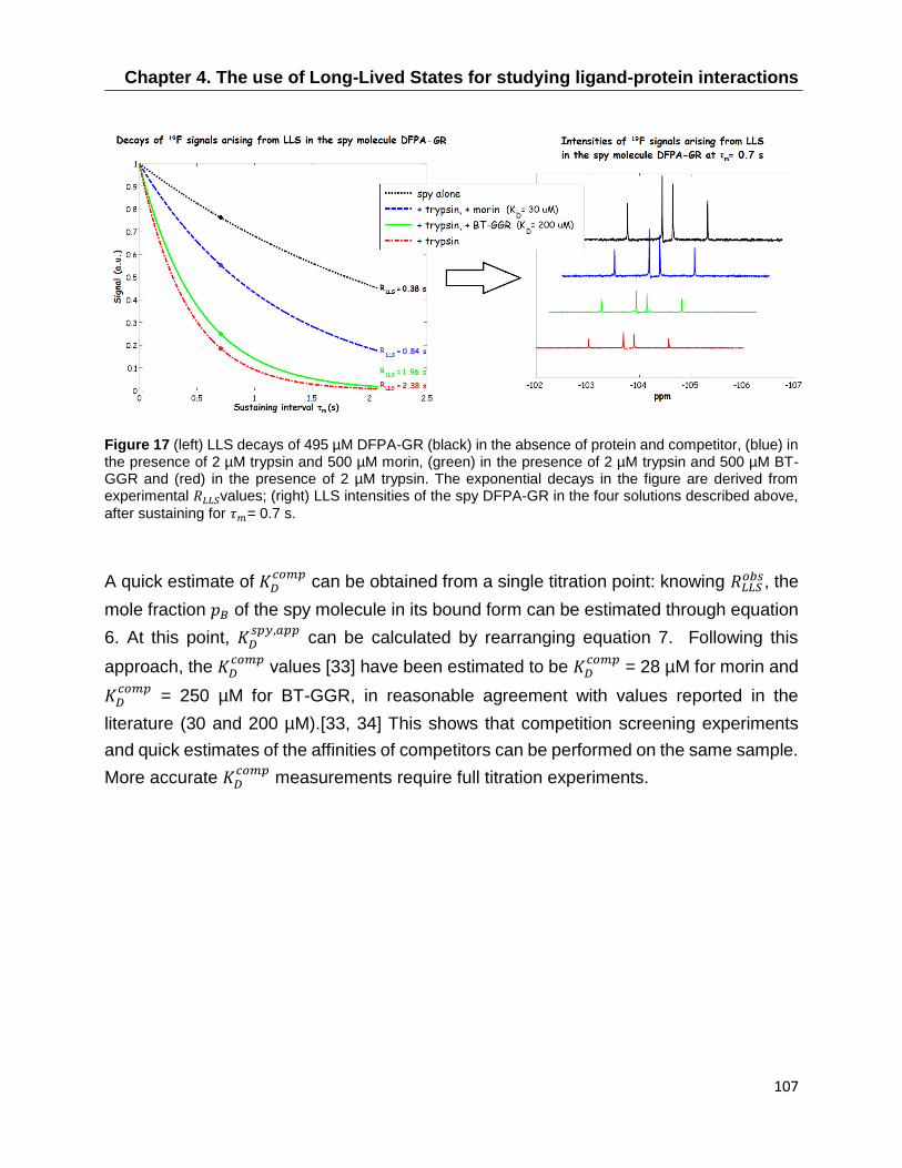
Chapter 4. The use of Long-Lived States for studying ligand-protein interactions
107
Figure 17 (left) LLS decays of 495 µM DFPA-GR (black) in the absence of protein and competitor, (blue) in the presence of 2 µM trypsin and 500 µM morin, (green) in the presence of 2 µM trypsin and 500 µM BT-GGR and (red) in the presence of 2 µM trypsin. The exponential decays in the figure are derived from experimental 𝑅𝐿𝐿𝑆values; (right) LLS intensities of the spy DFPA-GR in the four solutions described above,
after sustaining for 𝜏𝑚= 0.7 s.
A quick estimate of 𝐾𝐷𝑐𝑜𝑚𝑝
can be obtained from a single titration point: knowing 𝑅𝐿𝐿𝑆𝑜𝑏𝑠, the
mole fraction 𝑝𝐵 of the spy molecule in its bound form can be estimated through equation
6. At this point, 𝐾𝐷𝑠𝑝𝑦,𝑎𝑝𝑝
can be calculated by rearranging equation 7. Following this
approach, the 𝐾𝐷𝑐𝑜𝑚𝑝
values [33] have been estimated to be 𝐾𝐷𝑐𝑜𝑚𝑝
= 28 µM for morin and
𝐾𝐷𝑐𝑜𝑚𝑝
= 250 µM for BT-GGR, in reasonable agreement with values reported in the
literature (30 and 200 µM).[33, 34] This shows that competition screening experiments
and quick estimates of the affinities of competitors can be performed on the same sample.
More accurate 𝐾𝐷𝑐𝑜𝑚𝑝
measurements require full titration experiments.

4.6 Extending LLS ligand screening to 19F nuclei
108
Figure 18 (top) Proton spectrum of 495 µM DFPA-GR (spy); (bottom) Proton spectrum of 495 µM DFPA-
GR and 500 µM BT-GGR. The grey square shows the range where the signals of the α-protons of the
glycine residues occur.
Often, screening is performed by testing mixtures (also known as “cocktails”) of 3-10
putative competitors, in order to reduce experimental time and minimize protein
consumption. If one observes proton signals, such experiments need a careful choice of
the mixtures in order to avoid overlap of signals of the putative ligands with those of the
spy molecule. For example, figure 18 shows a comparison between the 1H spectra of the
spy molecule DFPA-GR alone and mixed with BT-GGR, a competitor with a similar
molecular structure. The overlap between the proton signals of the spy molecule and
those of the competitor are too severe to allow one to perform any competition screening
experiments. The problem can become even more severe when looking for weak binders.
Indeed, the larger the dissociation constants, the higher the required concentrations of the
competitors. In this context, 19F NMR has no rivals. It allows one to perform experiments
with high sensitivity while avoiding problems of overlap with protonated buffers and signals
of mixtures. The combination of the high sensitivity to binding phenomena offered by the
LLS method and the lack of overlap in 19F NMR can be put to good use for fragment-
based drug discovery.

Chapter 4. The use of Long-Lived States for studying ligand-protein interactions
109
References
1. B. Friguet, A. F. Chaffotte, L. Djavadiohaniance, and M. E. Goldberg,
Measurements of the True Affinity Constant in Solution of Antigen-Antibody
Complexes by Enzyme-Linked Immunosorbent-Assay. Journal of Immunological
Methods, 1985. 77(2): p. 305-319.
2. P. Schuck, Reliable determination of binding affinity and kinetics using surface
plasmon resonance biosensors. Current Opinion in Biotechnology, 1997. 8(4): p.
498-502.
3. J. E. Ladbury and B. Z. Chowdhry, Sensing the heat: The application of isothermal
titration calorimetry to thermodynamic studies of biomolecular interactions.
Chemistry & Biology, 1996. 3(10): p. 791-801.
4. C. A. Lepre, J. M. Moore, and J. W. Peng, Theory and applications of NMR-based
screening in pharmaceutical research. Chemical Reviews, 2004. 104(8): p. 3641-
3675.
5. B. J. Stockman and C. Dalvit, NMR screening techniques in drug discovery and
drug design. Progress in Nuclear Magnetic Resonance Spectroscopy, 2002. 41(3-
4): p. 187-231.
6. P. J. Hajduk, R. P. Meadows, and S. W. Fesik, NMR-based screening in drug
discovery. Quarterly Reviews of Biophysics, 1999. 32(3): p. 211-240.
7. L. Fielding, NMR methods for the determination of protein-ligand dissociation
constants. Progress in Nuclear Magnetic Resonance Spectroscopy, 2007. 51(4):
p. 219-242.
8. A. D. Bain, Chemical exchange in NMR. Progress in Nuclear Magnetic Resonance
Spectroscopy, 2003. 43(3-4): p. 63-103.
9. B. Meyer and T. Peters, NMR Spectroscopy techniques for screening and
identifying ligand binding to protein receptors. Angewandte Chemie-International
Edition, 2003. 42(8): p. 864-890.
10. H. M. Mcconnell, Reaction Rates by Nuclear Magnetic Resonance. Journal of
Chemical Physics, 1958. 28(3): p. 430-431.
11. S. B. Shuker, P. J. Hajduk, R. P. Meadows, and S. W. Fesik, Discovering high-
affinity ligands for proteins: SAR by NMR. Science, 1996. 274(5292): p. 1531-1534.
12. S. J. Perkins, L. N. Johnson, D. C. Phillips, and R. A. Dwek, The Binding of
Monosaccharide Inhibitors to Hen Egg-White Lysozyme by Proton Magnetic-
References
110
Resonance at 270 Mhz and Analysis by Ring-Current Calculations. Biochemical
Journal, 1981. 193(2): p. 553-572.
13. L. H. Lucas and C. K. Larive, Measuring ligand-protein binding using NMR diffusion
experiments. Concepts in Magnetic Resonance Part A, 2004. 20A(1): p. 24-41.
14. A. D. Chen and M. J. Shapiro, NOE pumping. 2. A high-throughput method to
determine compounds with binding affinity to macromolecules by NMR. Journal of
the American Chemical Society, 2000. 122(2): p. 414-415.
15. M. Mayer and B. Meyer, Characterization of ligand binding by saturation transfer
difference NMR spectroscopy. Angewandte Chemie-International Edition, 1999.
38(12): p. 1784-1788.
16. C. Dalvit, P. Pevarello, M. Tato, M. Veronesi, A. Vulpetti, and M. Sundstrom,
Identification of compounds with binding affinity to proteins via magnetization
transfer from bulk water. Journal of Biomolecular Nmr, 2000. 18(1): p. 65-68.
17. G. Valensin, T. Kushnir, and G. Navon, Selective and Non-Selective Proton Spin-
Lattice Relaxation Studies of Enzyme-Substrate Interactions. Journal of Magnetic
Resonance, 1982. 46(1): p. 23-29.
18. N. Salvi, R. Buratto, A. Bornet, S. Ulzega, I. R. Rebollo, A. Angelini, C. Heinis, and
G. Bodenhausen, Boosting the Sensitivity of Ligand-Protein Screening by NMR of
Long-Lived States. Journal of the American Chemical Society, 2012. 134(27): p.
11076-11079.
19. P. Ahuja, R. Sarkar, P. R. Vasos, and G. Bodenhausen, Diffusion Coefficients of
Biomolecules Using Long-Lived Spin States. Journal of the American Chemical
Society, 2009. 131(22): p. 7498-+.
20. C. Heinis, T. Rutherford, S. Freund, and G. Winter, Phage-encoded combinatorial
chemical libraries based on bicyclic peptides. Nature Chemical Biology, 2009. 5(7):
p. 502-507.
21. S. H. Ke, G. S. Coombs, K. Tachias, D. R. Corey, and E. L. Madison, Optimal
subsite occupancy and design of a selective inhibitor of urokinase. Journal of
Biological Chemistry, 1997. 272(33): p. 20456-20462.
22. R. Sarkar, P. R. Vasos, and G. Bodenhausen, Singlet-state exchange NMR
spectroscopy for the study of very slow dynamic processes. Journal of the
American Chemical Society, 2007. 129(2): p. 328-334.
23. B. Hess, C. Kutzner, D. van der Spoel, and E. Lindahl, GROMACS 4: Algorithms
for highly efficient, load-balanced, and scalable molecular simulation. Journal of
Chemical Theory and Computation, 2008. 4(3): p. 435-447.

Chapter 4. The use of Long-Lived States for studying ligand-protein interactions
111
24. C. Oostenbrink, A. Villa, A. E. Mark, and W. F. Van Gunsteren, A biomolecular
force field based on the free enthalpy of hydration and solvation: The GROMOS
force-field parameter sets 53A5 and 53A6. Journal of Computational Chemistry,
2004. 25(13): p. 1656-1676.
25. K. J. Kohlhoff, P. Robustelli, A. Cavalli, X. Salvatella, and M. Vendruscolo, Fast
and Accurate Predictions of Protein NMR Chemical Shifts from Interatomic
Distances. Journal of the American Chemical Society, 2009. 131(39): p. 13894-+.
26. K. Gopalakrishnan and G. Bodenhausen, Lifetimes of the singlet-states under
coherent off-resonance irradiation in NMR spectroscopy. Journal of Magnetic
Resonance, 2006. 182(2): p. 254-259.
27. G. Pileio and M. H. Levitt, Theory of long-lived nuclear spin states in solution
nuclear magnetic resonance. II. Singlet spin locking. Journal of Chemical Physics,
2009. 130(21).
28. G.C.K. Roberts, NMR of Macromolecules: A Practical Approach. 1993: IRL Press
at Oxford University Press.
29. C. Dalvit, M. Flocco, S. Knapp, M. Mostardini, R. Perego, B. J. Stockman, M.
Veronesi, and M. Varasi, High-throughput NMR-based screening with competition
binding experiments. Journal of the American Chemical Society, 2002. 124(26): p.
7702-7709.
30. A. Angelini, L. Cendron, S. Y. Chen, J. Touati, G. Winter, G. Zanotti, and C. Heinis,
Bicyclic Peptide Inhibitor Reveals Large Contact Interface with a Protease Target.
Acs Chemical Biology, 2012. 7(5): p. 817-821.
31. M. Renatus, W. Bode, R. Huber, J. Sturzebecher, and M. T. Stubbs, Structural and
functional analyses of benzamidine-based inhibitors in complex with trypsin:
Implications for the inhibition of factor Xa, tPA, and urokinase. Journal of Medicinal
Chemistry, 1998. 41(27): p. 5445-5456.
32. S. Jannin, A. Bornet, S. Colombo, and G. Bodenhausen, Low-temperature cross
polarization in view of enhancing dissolution Dynamic Nuclear Polarization in NMR.
Chemical Physics Letters, 2011. 517(4-6): p. 234-236.
33. R. Buratto, A. Bornet, J. Milani, D. Mammoli, B. Vuichoud, N. Salvi, M. Singh, A.
Laguerre, S. Passemard, S. Gerber-Lemaire, S. Jannin, and G. Bodenhausen,
Drug Screening Boosted by Hyperpolarized Long-Lived States in NMR.
Chemmedchem, 2014. 9(11): p. 2509-2515.
34. A. Checa, A. R. Ortiz, B. dePascualTeresa, and F. Gago, Assessment of solvation
effects on calculated binding affinity differences: Trypsin inhibition by flavonoids as

References
112
a model system for congeneric series. Journal of Medicinal Chemistry, 1997.
40(25): p. 4136-4145.
35. J. H. Ardenkjaer-Larsen, B. Fridlund, A. Gram, G. Hansson, L. Hansson, M. H.
Lerche, R. Servin, M. Thaning, and K. Golman, Increase in signal-to-noise ratio of
> 10,000 times in liquid-state NMR. Proceedings of the National Academy of
Sciences of the United States of America, 2003. 100(18): p. 10158-10163.
36. Y. Lee, H. F. Zeng, S. Ruedisser, A. D. Gosser, and C. Hilty, Nuclear Magnetic
Resonance of Hyperpolarized Fluorine for Characterization of Protein-Ligand
Interactions. Journal of the American Chemical Society, 2012. 134(42): p. 17448-
17451.
37. P. Mieville, P. Ahuja, R. Sarkar, S. Jannin, P. R. Vasos, S. Gerber-Lemaire, M.
Mishkovsky, A. Comment, R. Gruetter, O. Ouari, P. Tordo, and G. Bodenhausen,
Scavenging Free Radicals To Preserve Enhancement and Extend Relaxation
Times in NMR using Dynamic Nuclear Polarization (vol 49, pg 6182, 2010).
Angewandte Chemie-International Edition, 2010. 49(43): p. 7834-7834.
38. A. Comment, B. van den Brandt, K. Uffmann, F. Kurdzesau, S. Jannin, J. A. Konter,
P. Hautle, W. T. H. Wenckebach, R. Gruetter, and J. J. van der Klink, Design and
performance of a DNP prepolarizer coupled to a rodent MRI scanner. Concepts in
Magnetic Resonance Part B-Magnetic Resonance Engineering, 2007. 31B(4): p.
255-269.
39. S. Jannin, A. Bornet, R. Melzi, and G. Bodenhausen, High field dynamic nuclear
polarization at 6.7 T: Carbon-13 polarization above 70% within 20 min. Chemical
Physics Letters, 2012. 549: p. 99-102.
40. J. Milani, B. Vuichoud, A. Bornet, P. Mieville, R. Mottier, S. Jannin, and G.
Bodenhausen, A magnetic tunnel to shelter hyperpolarized fluids. Review of
Scientific Instruments, 2015. 86(2).
41. S. Bowen and C. Hilty, Rapid sample injection for hyperpolarized NMR
spectroscopy. Physical Chemistry Chemical Physics, 2010. 12(22): p. 5766-5770.
42. C. Dalvit, NMR methods in fragment screening: theory and a comparison with other
biophysical techniques. Drug Discovery Today, 2009. 14(21-22): p. 1051-1057.
43. R. Buratto, D. Mammoli, E. Chiarparin, G. Williams, and G. Bodenhausen,
Exploring Weak Ligand-Protein Interactions by Long-Lived NMR States: Improved
Contrast in Fragment-Based Drug Screening. Angewandte Chemie-International
Edition, 2014. 53(42): p. 11376-11380.

Chapter 4. The use of Long-Lived States for studying ligand-protein interactions
113
44. C. Dalvit, D. T. A. Hadden, R. W. Sarver, A. M. Ho, and B. J. Stockman, Multi-
selective one dimensional proton NMR experiments for rapid screening and binding
affinity measurements. Combinatorial Chemistry & High Throughput Screening,
2003. 6(5): p. 445-453.
45. C. W. Murray, M. G. Carr, O. Callaghan, G. Chessari, M. Congreve, S. Cowan, J.
E. Coyle, R. Downham, E. Figueroa, M. Frederickson, B. Graham, R. McMenamin,
M. A. O'Brien, S. Patel, T. R. Phillips, G. Williams, A. J. Woodhead, and A. J. A.
Woolford, Fragment-Based Drug Discovery Applied to Hsp90. Discovery of Two
Lead Series with High Ligand Efficiency. Journal of Medicinal Chemistry, 2010.
53(16): p. 5942-5955.
46. C. Dalvit, Ligand- and substrate-based F-19 NMR screening: Principles and
applications to drug discovery. Progress in Nuclear Magnetic Resonance
Spectroscopy, 2007. 51(4): p. 243-I.
47. G. Pileio, M. Carravetta, E. Hughes, and M. H. Levitt, The long-lived nuclear singlet
state of N-15-nitrous oxide in solution. Journal of the American Chemical Society,
2008. 130(38): p. 12582-+.
48. U. H. N. Durr, S. L. Grage, R. Witter, and A. S. Ulrich, Solid state F-19 NMR
parameters of fluorine-labeled amino acids. Part I: Aromatic substituents. Journal
of Magnetic Resonance, 2008. 191(1): p. 7-15.
49. S. L. Grage, U. H. N. Durr, S. Afonin, P. K. Mikhailiuk, I. V. Komarov, and A. S.
Ulrich, Solid state F-19 NMR parameters of fluorine-labeled amino acids. Part II:
Aliphatic substituents. Journal of Magnetic Resonance, 2008. 191(1): p. 16-23.
50. A. Checa, A. R. Ortiz, B. dePascualTeresa, and F. Gago, Assessment of solvation
effects on calculated binding affinity differences: Trypsin inhibition by flavonoids as
a model system for congeneric series. Journal of Medicinal Chemistry, 1997.
40(25): p. 4136-4145.

114

Chapter 5. Experimental procedures
115
5. Experimental procedures
All the experiments presented in this thesis were performed at 298 K on 500 MHz (11.7
T) or 600 MHz (16.4 T) Avance Bruker spectrometers equipped with 5 mm CryoProbes.
The following paragraphs give some details about ligand titrations, competition
experiments, fitting of data and synthesis of ligands. Further details can be found in
references [1-3].
5.1 Ligand titrations
Ligand titrations, as in figure 4 of Chapter 4, were performed by addition of small aliquots
(from 1 to 2 µL) of a concentrated ligand solution (from 150 to 200 mM) to 400 µL of a
buffered D2O solution containing the protein (from 10 to 20 µM). Lifetimes 𝑇𝐿𝐿𝑆 were
obtained by mono-exponential fitting of signal intensities observed with the LLS pulse
sequence described in Chapter 3, using 10 different spin-lock durations 0.5 s < 𝜏𝑚 < 5𝑇𝐿𝐿𝑆.
A short-cut can sometimes be used. For example, the relaxation rates 𝑅𝐿𝐿𝑆 reported in
figure 14 were obtained from ratios of the signal intensities observed using only two
different sustaining delays 𝜏𝑎 and 𝜏𝑏, repeating each of them twice in order to compare
four pairs of signal intensities 𝐼𝑎(𝜏𝑎)/𝐼𝑏(𝜏𝑏). In this case, the relaxation rates where
obtained from the ratio 𝑅𝐿𝐿𝑆 = (log(𝐼𝑎/𝐼𝑏))/(𝜏𝑏 − 𝜏𝑎). Typically, we used 𝜏𝑎 = 0.5 s, while
𝜏𝑏 was chosen in the vicinity of the estimated value of 𝑅𝐿𝐿𝑆.
Competition experiments were performed in the same manner. The only difference was
the presence of a potential competitor in the protein solution.
Ligand concentrations were carefully measured using the PULCON technique.[4]
5.2 Fitting of titration curves
The experimental data obtained were fitted to equation 6 of Chapter 4 to determine the
fraction of ligand in the bound form [𝑃𝐿] [𝐿]𝑡𝑜𝑡⁄ . Equation 7 was used to determine the
dissociation constant 𝐾𝐷.
For competition experiments, equation 7 of Chapter 4 gives the apparent dissociation
constant of the spy molecule 𝐾𝐷𝑠𝑝𝑦,𝑎𝑝𝑝
. Using this value, equation 8 of Chapter 4 gives the
dissociation constant of the competitor.

5.3 Hyperpolarized LLS experiments
116
5.3 Hyperpolarized LLS experiments
A detailed protocol for DNP-LLS experiments is described on page 95. Further details are
described in reference [2].
5.4 Chemical synthesis of ligands
Two ligands mentioned in this thesis, BT-GGR and DFPA-GR, are not commercially
available and were synthetized in our laboratory. Since the synthesis of BT-GGR is
described in the supporting information of reference [2], we describe here the preparation
of DFPA-GR.
The synthesis of 1,1-difluoro-1-phenylacetyl-Gly-Arg (DFPA-GR) was performed by solid-
phase peptide synthesis (SPPS) using 2-chlorotritylchloride resin and Fmoc protected
amino acids. The first step is a SN1 substitution of Fmoc-Arg(Pbf)-OH on the resin. All
remaining reactive 2-chlorotrityl groups were then capped with MeOH. The molecule was
obtained by coupling of Fmoc-protected Gly in the presence of HOBt and TBTU, followed
by deprotection of the N-terminus of the dipeptide. Finally, difluoro-phenyl-acetic acid was
attached at the N-terminus of the dipeptide. Cleavage from the resin, followed by
deprotection of the arginine side chain, afforded DFPA-GR.
N-Fmoc-Arg(Pbf)-O-resin (2): After swelling with dry DCM (80 mL) for 5 min, the 2-
chlorotrityl chloride resin (0.83 mmol.g-1, 1 equiv, 1 mmol, 1.2 g) was treated with a
solution of Fmoc-Arg(Pbf)-OH (1) (1.2 equiv, 1.2 mmol, 0.78 g) in dry DCM (10 mL) and
DIPEA (2.5 equiv, 6.23 mmol, 0.81 g) shaken at 125 rpm at room temperature for 2 hrs.
The reaction was performed in 4x10 mL filtration tubes with polyethylene fritters. MeOH
(10 mL) was added to cap the free sites, and the reaction mixture was shaken for 1. The
resin was washed with DCM (3 × 12 mL), DCM/MeOH 1:1 (3 × 12 mL), MeOH (3 × 12
mL), diethyl ether (3 x 12 mL) and dried for 12 hrs in vacuo to give the N-Fmoc-Arg(Pbf)-
O-resin (2).
N-Fmoc-Gly-Arg(Pbf)-O-resin (3): N-Fmoc-Arg(Pbf)-O-resin (2) was suspended in a
solution of 20% piperidine in DMF (10 mL) for 30 min and shaken to give the N-
deprotected resin. The resin was washed with DMF (4 × 10 mL) and DCM (4 × 10 mL).
Fmoc-Gly-OH (4 equiv, 4 mmol, 1.19 g), HOBt (4 equiv, 4 mmol, 0.54 g), TBTU (4 equiv,

Chapter 5. Experimental procedures
117
4 mmol, 1.29 g) and DIPEA (4 equiv, 4 mmol, 0.52 g) were dissolved in DMF (10 mL).
The solution was added to the N-deprotected resin. The reaction mixture was shaken at
room temperature for 3 hrs to give Fmoc-Gly-Arg(Pbf)-O-resin (3) which was washed with
DMF (4 × 10 mL).
Scheme 1. Synthesis of the 19F labelled ligand for trypsin 5.
DFPA-Gly-Arg(Pbf)-O-resin (4): Fmoc-Gly-Arg(Pbf)-O-resin (3) was suspended in a
solution of 20% piperidine in DMF (30 mL) for 30 min and shaken to give the N-
deprotected resin. The resin was washed with DMF (4 × 10 mL) and DCM (4 × 10 mL).

5.4 Chemical synthesis of ligands
118
Difluoro-phenyl-acetic acid (4 equiv, 4 mmol, 0.69 g), HOBt (4 equiv, 4 mmol, 0.54 g),
TBTU (4 equiv, 4 mmol, 1.29 g), and DIPEA (4 equiv, 4 mmol, 0.52 g) were dissolved in
DMF (30 mL). The solution was added to the N-deprotected resin. The reaction mixture
was shaken at room temperature for 3 hrs at 125 rpm to give DFPA-Gly-Arg(Pbf)-O-resin
(4) which was washed with DMF (4 × 10 mL) and DCM (4 × 10 mL).
DFPA-Gly-Arg (5): Cleavage from the resin and deprotection of the side-chain was
carried out with 10 mL TFA:H2O:TIS (95:2.5:2.5) for 3 hrs. TFA was then removed by
evaporation and the final product (5) was obtained after lyophilization.

Chapter 5. Experimental procedures
119
References
1. N. Salvi, R. Buratto, A. Bornet, S. Ulzega, I. R. Rebollo, A. Angelini, C. Heinis, and
G. Bodenhausen, Boosting the Sensitivity of Ligand-Protein Screening by NMR of
Long-Lived States. Journal of the American Chemical Society, 2012. 134(27): p.
11076-11079.
2. R. Buratto, A. Bornet, J. Milani, D. Mammoli, B. Vuichoud, N. Salvi, M. Singh, A.
Laguerre, S. Passemard, S. Gerber-Lemaire, S. Jannin, and G. Bodenhausen,
Drug Screening Boosted by Hyperpolarized Long-Lived States in NMR.
ChemMedChem, 2014. 9(11): p. 2509-2515.
3. R. Buratto, D. Mammoli, E. Chiarparin, G. Williams, and G. Bodenhausen,
Exploring Weak Ligand-Protein Interactions by Long-Lived NMR States: Improved
Contrast in Fragment-Based Drug Screening. Angewandte Chemie-International
Edition, 2014. 53(42): p. 11376-11380.
4. G. Wider and L. Dreier, Measuring protein concentrations by NMR spectroscopy.
Journal of the American Chemical Society, 2006. 128(8): p. 2571-2576.

120

6. Conclusions
121
6. Conclusions
he drug discovery and development process is a very long and expensive
pathway. It can take 12-15 years from the first, preliminary tests to the final
approval for marketing.
In the first stage of drug discovery, screening campaigns are usually performed in order
to identify a “hit compound”, which may bind to a macromolecular target and alter the
course of a disease. NMR offers a rich source of parameters that are sensitive to changes
in physical properties associated with binding. As consequence, a great variety of NMR
methods have been developed to perform screening experiments.
Long-Lived States (LLS) are nuclear spin states whose decay time constant 𝑇𝐿𝐿𝑆 can be
much longer than the longitudinal relaxation time 𝑇1. The goal of the present work was to
develop a new NMR strategy to study the interactions between ligands and proteins, by
exploiting some peculiar properties of the LLS.
In the regime of fast exchange on the NMR time scale, i.e., when the exchange between
the free and bound forms of a weak ligand is fast compared to the difference of their
resonance frequencies, the observable relaxation rate of a long-lived state associated with
a weak ligand results from a weighted average of the bound and free forms. As described
in Chapter 4, the contrast between the averaged LLS relaxation rate and the LLS
relaxation rate of the free ligand is proportional to the difference of the relaxation rates of
the free and the bound forms. Because of the long lifetimes of LLS in the free form and
the boosted LLS relaxation in the bound state, this difference is particularly large, making
the relaxation of long-lived states one of the most sensitive NMR parameters to ligand-
protein binding.
LLS have been successfully excited in glycine residues in short polypeptides in order to
quantify their affinities for protein targets. The use of competition experiments allowed the
study of binders which do not contain any spin system that can sustain a long-lived state.
Whenever there is no ligand that can carry a long-lived state, the functionalization of a
binder with a spin-pair label can provide a molecule that can be used as reporter in LLS
competition experiments. This strategy was used to synthetize a ligand containing a
bromo-thiophene group, which can carry an LLS on its two aromatic protons. The relatively
long 𝑇1 of these spins allowed us to perform a dissolution DNP experiment, where the
functionalized ligand was hyperpolarized, transferred to a conventional NMR
spectrometer and used as LLS reporter in competition experiments. This strategy allows
T

6. Conclusions
122
one to perform screening experiments with high contrast while working with low
concentrations of ligand and proteins.
The superior sensitivity of the LLS method can be exploited in order to quantify the affinity
of a weakly binding fragment to a protein target. By exploiting the LLS behaviour of a spy
molecule, we experimentally demonstrated that it is possible to measure dissociation
constants up to 12 mM, where most other biophysical techniques fail, including NMR
methods based on the observation of ligands.
We also explored LLS involving pairs of 19F nuclei to study binding phenomena. In a
custom-designed fluorinated ligand that binds trypsin, we have observed a ratio 𝑇𝐿𝐿𝑆 / 𝑇1
> 4. We found a dramatic effect on the LLS lifetime 𝑇𝐿𝐿𝑆 of the fluorinated ligand and great
contrasts have been observed between signals derived from 𝑇𝐿𝐿𝑆 with/without protein. This
fluorinated ligand has been successively used as spy molecule in competition
experiments, which allowed us to rank the affinities of arbitrary ligands that do not contain
any fluorine. The extension of LLS to pairs of 19F nuclei is an important achievement, since
fluorine detection allows one to perform screening campaigns without suffering from
problems due to overlapping signals. The combination of fluorine detection with DNP will
be the next frontier of screening by LLS. It could provide biophysical scientists with a very
sensitive and innovative tool to perform ligand-protein interaction studies.

123

124

Acknowledgements
125
Acknowledgements
The first ‘thanks’ goes to the members of my thesis committee for taking the time to read
this manuscript and judge my work: Prof. Lyndon Emsley, president of the jury, Dr.
Wolfgang Jahnke and Dr. Elisabetta Chiarparin, external examiners, and Prof. Kai
Johnsson, internal examiner. Together with my advisor and co-advisor, I guess that in
twenty years they still will be the only ones to have read entirely this manuscript.
I thank immensely my advisor Prof. Geoffrey Bodenhausen for giving me the opportunity
to work in his lab. His unattainable knowledge and enthusiasm drove me (and many other
PhD students and postdocs) during these four years, showing how the combination of
fantasy, originality and rigor is the best recipe to perform successful research.
I am indebted to my co-advisor Prof. Claudio Dalvit, who helped and advised me in many
circumstances, despite of the constant geographic distance. The trips to Neuchatel and
the hours spent in front of his spectrometers allowed me to learn not only about scientific
concepts, but also about the approach to science of a person who has a deep experience
both at academic and industry level.
I would really like to thank Astex Pharmaceuticals for the fruitful collaboration. They
provided us not only with precious proteins and molecules, but also with their priceless
knowledge of the pharmaceutical field. In this context, I thank in particular Dr. Glyn
Williams, who sustained the collaboration and welcomed me during my visit to their site
in Cambridge. It has been really a great pleasure to meet him.
From now on, I want to spend a couple of words for all the people I met during this amazing
experience, assigning a funny nickname at the end of the description. I would like to start
with Dr. Simone Ulzega, who has been the first person to welcome me in Lausanne in the
far 2011 during my Erasmus experience. He probably remembers those first days when I
was almost not able to communicate in English and consequently he was my Italian
lifebelt. I will never forget our scrupulous analysis of the Serie A and Champions league
results and, above all, his innate skills in mimic the way of kicking the ball of famous
players (not always with positive results). Football mentor.

Acknowledgements
126
I thank also Dr. Nicola Salvi, nicknamed ‘Chamois of Abruzzo’ for his hiking skills, for
making possible one of the best works I had the privilege to co-author. I shared with him
also my first transatlantic flight and my first exploration of California (and my first US fine!).
Unfortunately, he is a supporter of Inter, but everybody knows that nobody is perfect!
NoInter,please.
A big thanks goes also to Dr. Diego Carnevale. He is a great expert in solid state NMR, a
field which is very far from my works. As consequence, we almost did not share any
scientific project. Despite of this, he has always been very kind and ready to have fun. He
is also a supporter of Inter, but some beers can make me forget about it. Great Escape.
When I arrived in Switzerland, I had never touched seriously an NMR spectrometer before.
Here, I have been very lucky to meet Dr. Aurelien Bornet, who had a huge patience while
introducing me to the NMR world. NobelPriceForPatience (but do not profit, he knows how
to drive a tank).
He is currently a member of the Swiss team. I know you do not know what the Swiss team
is, but this is a motivation to keep reading these last pages.
During my first Swiss period I met also Dr. Veronika Vitzthum and Dr. Marc Caporini. I
would like to thank them for the happy atmosphere they were creating every day in the
lab. I will remember forever the fantastic gastronomic hiking session we had together. I
thank also Dr. Pascal Mieville and Anto Barisic for maintaining our spectrometers and to
solve every kind of hardware issue. Precious people.
I shared both my exchange period and the first part of my PhD with Dr. Takyua Segawa.
He made at least fifty phone calls while I was looking for an apartment and he was
managing many everyday tasks in the lab. I have never understood if his efficiency was
due to his Swiss component or to the Japanese one. I thank him also for organizing
afternoon breaks at the cafeteria, everyday at 16 o’clock. Swiss watch.
During these four years, I had the opportunity to discover India through two enthusiastic
India representatives: Dr. Srinivas Chithalapalli and Maninder Singh. I still remember our
chats about India and Europe during lunch time. They have been funny colleagues and
great hosts during my trip in Amritsar. Indian guides.

Acknowledgements
127
Also China brought its contribution during this multicultural experience. Shutao Wang has
been a very nice and funny colleague, while Xiao Ji makes me still uncomfortable when
he speaks French better than me! But I can accept to be beaten by a Chinese who does
not fear to try Swiss fondue and to get home drunk after a wine contest! Great walls.
I shared my office for more than one year with Dr. Pavel Kaderavek. He is a very nice
person and a good scientist. I thank him for having kept constantly active our office during
this period (weekends included). I thank also Dr. AJ Perez-Linde for having contributed to
very funny moments in the lab life. Right?
I would like to thank Dr. Sami Jannin, Jonas Milani and Basile Vuichoud for contributing
to the nice atmosphere of the lab and for the fruitful collaboration in one of my projects.
Coming back to the funny part, they are all members of the Swiss team, which wants to
convince people that Switzerland is better than other many countries not only for cheese,
chocolate and banks. They want to convince people that Switzerland is better also for
wines and soccer skills…and, above all, they want to convince Italian people that
pineapple pizza is good. Reckless.
I want to thank a lot also my current office-mates. Daniele Mammoli and Estel Canet are
for me not only nice colleagues, but primarily great friends. We shared not only a space
and some scientific projects, but also very nice experiences. Dinners. Parties. Bottles of
wine. Venetian dialect songs. I will never forget our road trip in California, Nevada and
Arizona. Daniele’s obsession for optimization. Estel’s liveliness. Milestones.
I am indebted to Béatrice Bliesener-Tong and Anne Lene Odegaard for the precious work
they carried out. Whenever I had a bureaucratic problem or doubt, they knew how to fix
it. Swiss efficiency.
Before to conclude, I would like to thank all my friends in Lausanne, because PhD studies
are not only four years spent in a lab. PhD studies are four years of life. Four years of bad
and nice emotions. For these reasons, I have to thank my family. They have always
supported me, letting me freely choose what I really wanted to do and being there
whenever I needed them. I would like to thank also Alessia. With her, I got convinced that
the best part of my life is coming now.

Acknowledgements
128
I am sure you arrived to read this line skipping several parts of this wonderful manuscript.
Anyway, I am glad that you read at least a small part of it. So, thank you!
Lausanne, September 2015

129
CURRICULUM VITAE
Personal information
Name Roberto BURATTO
Address Avenue Jomini 2, 1004 Lausanne
Switzerland
Contacts Tel.: +41 (0)78 700 59 82
Email: [email protected]
Birthplace/date Soave (Italy), 07.09.1987
Nationality Italian
Languages Italian (mother tongue), English (fluent), French (basic)
Civil Status Single
Education and professional history 2012 – Present PhD student
“Exploring Ligand Affinities for Proteins by NMR of Long-Lived
States”
Biomolecular Magnetic Resonance Lab (Prof. G. Bodenhausen)
Ecole Polytechnique Fédérale de Lausanne (EPFL), Switzerland
2011 Internship
“Long-lived nuclear spin states: new probes for the investigation of
biomolecular dynamics and interactions”
Biomolecular Magnetic Resonance Lab (Prof. G. Bodenhausen)
Ecole Polytechnique Fédérale de Lausanne (EPFL), Switzerland
2009 – 2011 M.Sc. in Chemistry
University of Padova, Italy
Master thesis: “Long-lived nuclear spin states: new probes for the
investigation of biomolecular dynamics and interactions”
2006 – 2009 B.Sc. in Chemistry
University of Padova, Italy
Bachelor thesis: “DJ1-DAQ conjugates in Parkinson disease (a
topological study with molecular dynamic simulations)”

130
Awards 2013
Prize for the best poster, 49th International Conference on Medicinal
Chemistry, Nice, France
2015
2015 SCNAT/SCS Chemistry Travel Award, offered by the Swiss
Chemical Society and the Swiss Society for Foood and Enviromental
Chemistry
Professional and research experience EPFL - Investigation of fundamental aspects of NMR spectroscopy in liquid
states
- Development of NMR experimental methods
o Detection of ligand-protein binding with new strategies, which
allow to save materials and to work with cheaper proteins
o Definition of chemical strategies to render screening methods
always applicable
o Combination of new screening methods with innovative techniques
(dissolution-DNP) to increase the sensitivity of the experiments
o Development of screening strategies based on 19F detection, which
allow to speed-up the screening processes
o Investigation of relaxation properties of water in gas phase
o Development of strategies to detect para-water in bulk
- Supervision of several student projects
- Organization of interdisciplinary projects for students, to be developed
in different EPFL laboratories
- Teaching at all levels (B.Sc, M.Sc. and Ph.D)
Programming skills
- Experience with Matlab, Origin
- Experience with Bruker NMR software for implementation/modification of pulse sequences
- Basic experience with programming languages as Pascal, Java
Patent applications

131
EP20110793393, Method for the nmr based determination of the affinity of drugs for a target
protein , EPFL
Hobbies and interests Passionate of wines and agriculture, traveling, sports. I am currently the vice-president of
Italaus, an association of Italian students and PhDs (recognized by EPFL) for the promotion of
the Italian culture in Lausanne.
List of Publications
1. Bornet A., Milani J., Wang S., Mammoli D., Buratto R., Salvi N., Segawa T.F.,
Vitzthum V., Mieville P., Chintalapalli S., Perez-Linde A.J., Carnevale D., Jannin S.,
Caporini M., Ulzega S., Rey M., Bodenhausen G. Dynamic Nuclear Polarization and
Other Magnetic Ideas at EPFL, Chimia (2012), 66(10):734-740.
2. Salvi N., Buratto R., Bornet A., Ulzega S., Rentero Rebollo I., Angelini A., Heinis C.,
Bodenhausen G. Boosting the Sensitivity of Ligand-Protein Screening by NMR of Long-
Lived States, J Am Chem Soc (2012), 134(27):11076-11079.
3. Buratto, R., Bornet, A., Milani, J., Mammoli, D., Vuichoud, B., Salvi, N., Singh, M.,
Laguerre, A., Passemard, S., Gerber-Lemaire, S., Jannin, S. and Bodenhausen G. Drug
Screening Boosted by Hyperpolarized Long-Lived States in NMR, ChemMedChem
(2014), 9: 2509-2515.
4. Buratto, R., Mammoli, D., Chiarparin, E., Williams, G. and Bodenhausen, G. Exploring
Weak Ligand-Protein Interactions by Long-Lived NMR States: Improved Contrast in
Fragment-Based Drug Screening, Angew Chem Int Ed (2014), 53: 11376-11380.
5. Mammoli D., Salvi N., Milani J., Buratto R., Bornet A., Swhgal A. A., Canet E.,
Pelupessy P., Carnevale D., Jannin S., and Bodenhausen G. On the path to para-water
in bulk: overcoming proton exchange and other hurdles, Phys Chem Chem Phys (2015),
in press.
Conferences
1. EUROMAR Conference, Dublin, Ireland, June 30th-July 5th, 2012.

132
Poster title: Boosting Sensitivity of Ligand-Protein Screening by NMR of Long-Lived
States
2. ENC Conference, Asilomar, California, April 14-19th, 2013.
Poster title: Protein-Ligand Affinity using Long-Lived States and Long-Lived
Coherences
3. RICT Conference, Nice, France, July 3-5th, 2013.
Poster title: Towards DNP-Enhanced LLS and LLC for Ligand Screening
4. SCS fall meeting, Lausanne, Switzerland, September 6th, 2013.
Poster title: Protein-Ligand Affinity using Long-Lived States and Long-Lived
Coherences
5. ENC Conference, Boston, USA, March 23-28th, 2014.
Poster title: DNP-Enhanced Ligand-Protein Screening by NMR of Long-Lived States
6. RSC NMR DC, Spring Meeting 2014, Cambridge, UK, April 10-11th, 2014.
Oral presentation: Beyond the millimolar range: measuring ultra-weak ligand-protein
affinities using NMR of Long-Lived States
7. EUROMAR Conference, Zurich, Switzerland, June 29th-July 3rd, 2014.
Poster title: Exploring weak ligand-protein interactions by Long-Lived States in NMR:
improved contrast in Fragment-Based Drug Screening
8. FBLD Conference, Basel, Switzerland, September 21-24th, 2014.
Poster title: Exploring weak ligand-protein interactions by Long-Lived States in NMR:
improved contrast in Fragment-Based Drug Screening
9. NMRS Conference, Amritsar, India, March 6-9th, 2015.
Invited oral presentation: Ligand-Protein Interaction Studies by NMR of Long-Lived
States
10. ENC Conference, Asilomar, California, April 19-24th, 2015.
Oral presentation: Ligand-Protein Screening by Long-Lived States of Fluorine-19
Nuclei
11. EUROMAR Conference, Prague, Czech Republic, July 5-10th, 2015.
Oral presentation: Long-Lived States of pairs of Fluorine-19 Nuclei: a new tool for
Ligand-Protein Screening