Exploring Crypto Dark Matter:

New Simple PRF Candidates and Their Applications∗

Dan Boneh† Yuval Ishai‡ Alain Passelegue§ Amit Sahai§ David J. Wu†

Abstract

Pseudorandom functions (PRFs) are one of the fundamental building blocks in cryptography.We explore a new space of plausible PRF candidates that are obtained by mixing linear functionsover different small moduli. Our candidates are motivated by the goals of maximizing simplicityand minimizing complexity measures that are relevant to cryptographic applications such assecure multiparty computation.

We present several concrete new PRF candidates that follow the above approach. Ourmain candidate is a weak PRF candidate (whose conjectured pseudorandomness only holds foruniformly random inputs) that first applies a secret mod-2 linear mapping to the input, and thena public mod-3 linear mapping to the result. This candidate can be implemented by depth-2ACC0 circuits. We also put forward a similar depth-3 strong PRF candidate. Finally, we presenta different weak PRF candidate that can be viewed as a deterministic variant of “LearningParity with Noise” (LPN) where the noise is obtained via a mod-3 inner product of the inputand the key.

The advantage of our approach is twofold. On the theoretical side, the simplicity of our can-didates enables us to draw natural connections between their hardness and questions in complex-ity theory or learning theory (e.g., learnability of depth-2 ACC0 circuits and width-3 branchingprograms, interpolation and property testing for sparse polynomials, and natural proof barri-ers for showing super-linear circuit lower bounds). On the applied side, the “piecewise-linear”structure of our candidates lends itself nicely to applications in secure multiparty computation(MPC). Using our PRF candidates, we construct protocols for distributed PRF evaluation thatachieve better round complexity and/or communication complexity (often both) compared toprotocols obtained by combining standard MPC protocols with PRFs like AES, LowMC, orRasta (the latter two are specialized MPC-friendly PRFs). Our advantage over competing ap-proaches is maximized in the setting of MPC with an honest majority, or alternatively, MPCwith preprocessing.

Finally, we introduce a new primitive we call an encoded-input PRF, which can be viewedas an interpolation between weak PRFs and standard (strong) PRFs. As we demonstrate, anencoded-input PRF can often be used as a drop-in replacement for a strong PRF, combiningthe efficiency benefits of weak PRFs and the security benefits of strong PRFs. We conclude byshowing that our main weak PRF candidate can plausibly be boosted to an encoded-input PRFby leveraging error-correcting codes.

∗This is a preliminary full version of [BIP+18]†Stanford University. Email: dabo, dwu4@cs.stanford.edu‡Technion. Email: yuvali@cs.technion.ac.il. Work done in part while visiting UCLA.§UCLA. Email: alain.passelegue@inria.fr, sahai@cs.ucla.edu

1

1 Introduction

In this paper, we continue a line of work on constructing low-complexity pseudorandom functions.We explore a new space of simple candidate constructions that enjoy several advantages over existingcandidates. We start with some relevant background.

As discussed in [ABG+14], there are two primary paradigms for designing cryptographic prim-itives. The “theory-oriented” or “provable security” approach is to develop constructions whosesecurity can be provably reduced to the hardness of well-studied computational problems (e.g., fac-toring, discrete log, or learning with errors). The second and “practice-oriented” approach aims atobtaining efficient constructions for specific functionalities (e.g., block ciphers or hash functions).Here, designers typically try to maximize concrete efficiency at the expense of relying on heuristicarguments and prior experience to argue security. But ultimately, confidence in the underlyingsecurity assumptions or cryptographic designs only grows if they withstand the test of time.

There are several limitations to these approaches. On the one hand, both the efficiency and thestructure of provably-secure constructions are inherently limited by the underlying computationalproblems. This leads to constructions that are far less efficient than those obtained from thepractice-oriented approach. On the other hand, despite the efficiency of practical constructions,their designs are often complex, thereby complicating their analysis. Consequently, it is difficultto argue whether the lack of cryptanalysis against practical constructions is due to their actualsecurity or due to the complexity of their design. The structure of both types of constructionsoften makes them poorly suited as building blocks for cryptographic applications that are differentfrom the ones envisioned by their designers (e.g., secure multiparty computation).

In this work, we depart from these traditional approaches and consider a surprisingly unexploredspace of cryptographic constructions. Our approach is driven by simplicity, and aims at circum-venting some of the limitations of the existing approaches. Our hope is to obtain constructionsthat are (1) relatively easy to describe and analyze, (2) concretely efficient, and (3) well-suited fordifferent applications. In particular, we aim at relying on assumptions that are simple to state, andyet at the same time, breaking them would likely require new techniques that may themselves haveother applications. In a sense, the assumptions we introduce have a win-win flavor and can be ofindependent interest beyond the cryptographic community (e.g., to complexity theorists, learningtheorists, or mathematicians). A notable example for prior work in this direction is Goldreich’s pro-posal of a simple one-way function candidate [Gol00], which had an unexpected impact in differentareas of cryptography and beyond (see [App13] for a survey). More closely relevant to this work,the works of Miles and Viola [MV12] and (especially) Akavia et al. [ABG+14] proposed heuristicconstructions of simple pseudorandom functions and proved their security against natural classesof attacks, without reducing their security to any previously studied assumption.

What do we mean by simplicity? The concrete direction we take is exploring whether theidea of mixing linear functions over different moduli can be a source of hardness in the contextof secret-key cryptographic primitives. Our starting observation is that computing the sum of mbinary-valued variables modulo 3 is actually a high-degree polynomial over Z2. More precisely,the mapping function map : 0, 1m → Z3 where map(x) :=

∑i∈[m] xi (mod 3) is a polynomial of

high-degree over the binary field Z2 (but a simple linear function over Z3). Surprisingly, this simple

2

idea of mixing different small moduli enables new constructions of “piecewise-linear1” symmetricprimitives that are conceptually simple to describe, can plausibly achieve strong security guarantees,and minimize complexity measures that are relevant to natural cryptographic applications.

Our focus: pseudorandom functions. In this work, we focus specifically on pseudorandomfunctions (PRFs) [GGM86]—one of the most fundamental building blocks of modern cryptography.Our primary focus is on weak pseudorandom functions: namely, functions whose behavior looksindistinguishable from that of a random function to any adversary who only observes the input-output behavior of the function on random domain elements. Since weak PRFs cannot replacestandard (or strong) PRFs in all cryptographic applications, we then show how our constructioncan be adapted to yield a new primitive we call an encoded-input PRF. An encoded-input PRFis defined similarly to a standard (strong) PRF, except that its input domain is restricted toan efficiently recognizable set. Encoded-input PRFs can be viewed as an intermediate primitivebetween strong PRFs and weak PRFs that combines the security advantages of the former andefficiency advantages of the latter. Indeed, we show that in many cases they can be used as areplacement for a strong PRF. At the same time, we exhibit simple candidates of encoded-inputPRFs in complexity classes where strong PRFs are not known to exist. Finally, a unique feature ofour new PRF candidates is that they are very “MPC-friendly.” As we show in Section 6, in somenatural settings of secure computation, our PRFs can be computed more efficiently in a distributedfashion compared to standard block ciphers like AES and even custom-built MPC-friendly blockciphers like LowMC [ARS+15] or Rasta [DEG+18].

Previous work on simple PRFs. Before describing our contributions, it is useful to surveysome closely relevant previous works on low-depth PRFs (see Sections 1.2 and 3.2 for a broadersurvey). We denote by AC0 the class of polynomial-size, constant-depth circuits with unboundedfan-in AND, OR, and NOT gates and by ACC0[m] the class of such circuits that can additionallyhave unbounded fan-in MODm gates, which return 0 or 1 depending on whether the sum of theirinputs is divisible by m. We denote by ACC0 the union over all m of ACC0[m].

With the goal of minimizing the depth complexity of weak PRFs, Akavia et al. [ABG+14]proposed the first candidate that can be computed by ACC0[2] circuits. More precisely, theircandidate construction can be computed by depth-3 circuits in which the first layer consists of MOD2

gates computing a matrix-vector product Ax, where A ∈ Zn×n2 is the secret key and x ∈ Zn2 is theinput. The second and third layer define a public DNF formula. While the Akavia et al. candidatecould plausibly provide exponential security,2 Bogdanov and Rosen [BR17] recently showed thatthis candidate (on n-bit inputs) can be computed by a rational function of degree O(log n), whichin turn gives rise to a quasi-polynomial time attack. Their work also raises the question of comingup with an explicit function g for which g(Ax+b) is a weak PRF with better than quasi-polynomialsecurity. Applebaum and Raykov [AR16] show that low-complexity PRFs can be based on one-wayness assumptions. In particular, under a variant of Goldreich’s one-wayness assumption [Gol00],they present a weak PRF with quasi-polynomial security that can be implemented (on any fixedkey) by depth-3 AC0 circuits.

1In our context, we use the term “piecewise-linear” to refer to the fact that our pseudorandom function candidatescan be expressed as a composition of linear functions over different moduli.

2Roughly speaking, we say that a weak PRF is exponentially secure if the distinguishing advantage of any adversary(modeled as a Boolean circuit) of size 2λ is bounded by 2−Ω(λ).

3

These recent results leave several open questions regarding the complexity of low-depth (weak)PRFs. First, even if one settles for quasi-polynomial time security, there is no proposed PRFcandidate of any kind that can be realized by depth-2 circuits over any standard basis. Whenrestricting attention to (weak) PRFs that offer a better level of security, the situation is evenworse. While it is known that weak PRFs with better than quasi-polynomial security do not existin AC0,3 and that strong PRFs with similar security do not exist in ACC0[p] for any prime p,4 itis plausible that weak PRFs with exponential security could still exist in ACC0[2]. But to the bestof our knowledge, no such candidates have been suggested. If we do settle for quasi-polynomialsecurity, then the result of Kharitonov [Kha93, Theorem 9] (resp., Viola [Vio13, Theorem 11])gives a weak PRF in AC0 (resp., strong PRF in ACC0[p] for any p) based on the hardness offactoring. This raises the question of whether it is possible to construct (weak or strong) PRFswith exponential (or even just better than quasi-polynomial) security in ACC0. In this work, wepropose a new candidate weak PRF that can be computed by depth-2 ACC0 circuits. Our candidateis conceptually simple and can plausibly satisfy exponential security, thus addressing both of theabove challenges simultaneously. We also propose other variants of this candidate, including acandidate for an exponentially secure strong PRF that can be computed by depth-3 ACC0 circuits.We provide a comparison of the known positive and negative results for weak and strong PRFs indifferent complexity classes in Table 1.

Complexity Class

Circuit Depth AC0 ACC0[p] ACC0[m]

Depth 2Weak PRF (§3)(exponential)

Depth 3Weak PRF [AR16] Weak PRF [ABG+14] Strong PRF (§7.3)(quasi-polynomial) (quasi-polynomial) (exponential)

Depth > 3Weak PRF [Kha93] Strong PRF [Vio13](quasi-polynomial) (quasi-polynomial)

Lower Bound

No weak PRF with No strong PRF withbetter than better than

quasi-polynomial quasi-polynomialsecurity [LMN89] security [CIKK16]

Table 1: Comparison of positive and negative results for low-complexity PRF candidates. Wewrite ACC0[p] to denote the class AC0 with MODp gates for a prime p and ACC0[m] to denote theclass AC0 with MODm gates for any integer m. For each candidate, we denote in parenthesis theirsecurity (i.e., quasi-polynomial security or exponential security). The entries shown in bold (theright-hand column) are from this work.

3Specifically, the classic learning result of Linial et al. [LMN89] showed that AC0 circuits can be learned from randomexamples in quasi-polynomial time.

4The recent learning result by Carmosino et al. [CIKK16] showed that for any prime p, ACC0[p] circuits can be learnedusing membership queries in quasi-polynomial time. Extending this result to the setting of learning from uniformlyrandom examples (without membership queries) or to composite moduli seems challenging.

4

1.1 Our Contributions

In this section, we give a more detailed overview of the main results of this paper.

New weak PRF candidates. We put forward several new (weak) PRF candidates that mixlinear functions over different moduli. We start by describing our most useful candidate, and willdiscuss other variants later. Our primary weak PRF candidate follows a very similar design philos-ophy as that taken by Akavia et al. [ABG+14]. Recall first that in the Akavia et al. construction,the secret key is a matrix A ∈ Zm×n2 and the input is a vector x ∈ Zn2 . The output of the PRFis defined as FA(x) := g(Ax), where the function g is a non-linear mapping (in the case of theAkavia et al. construction, the function g is a “tribes” function and can be expressed as a DNFformula). In our setting, we adopt the same high-level structure, but substitute a different andconceptually simpler non-linear function g. In our candidate, we define the non-linear function tobe the function that interprets the binary outputs of Ax as 0/1 values over Z3, and the output ofthe function is simply the sum of the input values over Z3. This gives a simple candidate answerto the aforementioned open question of Bogdanov and Rosen [BR17].

Specifically, we define the mapping function map : 0, 1m → Z3 that maps y ∈ 0, 1m 7→∑i∈[m] yi (mod 3). Our weak PRF candidate (with key A) is then defined as

FA(x) := map(Ax) . (1.1)

We formally introduce our candidate (and discuss several generalizations5) in Section 3. We stateour formal conjectures regarding the hardness of our candidate in Section 3.1. There are severalproperties of our weak PRF candidate that we want to highlight:

• Conceptual simplicity. Our candidate is conceptually very simple to describe. It reducesto computing a (secret) matrix-vector product over Z2, reinterpreting the output vector asa 0/1 vector mod-3 and then computing the sum of its components. The simplicity of ourconstruction is fairly apparent compared to block cipher candidates like AES or number-theoretic constructions of PRFs. In spite of its simplicity, to the best of our knowledge, sucha candidate has not previously been proposed, let alone studied.

• Low complexity. Our candidate can be computed by depth-2 ACC0[2, 3] circuits. Moreprecisely, the first layer consists entirely of MOD2 gates to compute the matrix-vector productAx, and the second layer consists of two MOD3 gates that computes the binary representationof the output. We refer to Remark 3.10 for a more precise definition.

• MPC friendliness. The simplicity of our candidate also lends itself nicely for use in MPCprotocols. In Section 6, we give an efficient protocol that enables distributed evaluationof our PRF in a setting where both the key and the input are secret-shared. We discussthis further in the sequel. As we show in Table 2 and Table 3, the round complexity andcommunication complexity of our distributed evaluation protocol outperform existing MPCprotocols for distributed evaluation of not only AES, but even those for MPC-friendly blockciphers like LowMC [ARS+15] and Rasta [DEG+18]. This applies both to the 3-party casewith one corrupted party and (especially) to the case of secure 2-party computation withpreprocessing.

5An immediate generalization is replacing 2 and 3 by different numbers. However, the particular choice of 2 and 3turns out to be the most useful for our purposes. A more useful generalization replaces the above choice of map bya suitable compressive mod-3 linear mapping, which yields weak PRF candidates with a longer output.

5

Cryptanalysis. In Section 4, we consider several classic cryptanalytic techniques on our weakPRF candidate. While our analysis is by no means exhaustive, we are able to rule out several classesof attacks, thereby providing some confidence into the security of our new candidate. Following thework of Akavia et al. [ABG+14], we focus on two primary classes of attacks:

• Lack of correlation with fixed function families. First, we rule out the learning-typeattacks of Linial et al. [LMN89] by showing that there are no fixed function families of expo-nential size that are noticeably correlated with our PRF candidate (previously, Linial et al.showed that for all AC0 functions, there exists a quasi-polynomial-size function family suchthat any AC0 function is noticeably correlated with a function in that class; this implies aquasi-polynomial time learning algorithm for AC0).

• Inapproximability by low-degree polynomials. Next, we show that there does notexist a low-degree polynomial approximation to our PRF candidate. Our argument herefollows from the well-known Razborov-Smolensky lower bounds [Raz87, Smo87] for ACC0

circuits, which say that for distinct primes p, q, the MODp function cannot be computed(or even approximated) by a polynomial-size circuit in ACC0[q]. We conjecture that theRazborov-Smolensky lower bounds also generalize to rule out low-degree rational approxima-tions. Namely, for distinct primes p, q, there does not exist a low-degree rational functionthat approximates MODp gates sufficiently well over GF(q`) for any ` (Conjecture 4.3). Webelieve that this question is of independent interest from a complexity-theoretic perspective,and leave it as an interesting challenge.

Given the above, we conjecture that our main weak PRF candidate is exponentially secure. Wehope that our exploratory analysis will encourage further study and refinement of our conjectures.

Additional PRF candidates. In addition to our main weak PRF candidate (Eq. (1.1)), we alsopropose a similar strong PRF candidate and an alternative weak PRF candidate.

• Strong PRF candidate in depth-3 ACC0. Our weak PRF candidate from Eq. (1.1) is nota strong PRF, and as we discuss later in this section and in Section 5.3, there is a non-adaptiveattack against our candidate. Moreover, in Appendix B.1, we describe a more general adaptiveattack that rules out many natural strong PRF constructions in depth-2 ACC0. However, theexisting attacks do not seem to extend to depth-3 ACC0, and in Section 7.3, we propose astrong PRF candidate in depth-3 ACC0 that relies on the same general technique of mixinglinear operations over different moduli (Construction 7.9, Remark 7.14).

Our depth-3 strong PRF candidate is obtained by first applying a public random mod-3linear mapping to the input, taking the binary decomposition of the resulting vector (toobtain a mod-2 vector), and then evaluating our weak PRF candidate F (Equation 1.1) onthe decomposed mod-2 vector. Essentially, we can view the initial mod-3 mapping and binarydecomposition as computing a public “encoding” of the input. The strong PRF candidateis then essentially our weak PRF applied to the encoding of the input. The overall PRFcomputation thus consists of a mod-3/mod-2/mod-3 computation, where the mod-3 mappingsare public and the mod-2 mapping is secret.

Specifically, let G ∈ Zn′×n

3 be a fixed public matrix, bin : Zn′3 → 0, 12n′

be the component-wise binary decomposition function (that maps each Z3 component into two bits correspond-ing to the binary representation of the component). The PRF key is a matrix A ∈ Zm×2n′

2

6

and on input x ∈ 0, 1n, the output is

F′A(x) := FA(bin(G · x)) , (1.2)

where FA is our weak PRF candidate from Eq. (1.1). To the best of our knowledge, thisis the first strong PRF candidate computable by a depth-3 circuit that plausibly providesexponential (or even better than quasi-polynomial) security. We discuss this candidate andits applications in Section 7.3.

• An alternative weak PRF candidate. As we discuss below (and in Section 6), the struc-ture of our main candidate enables efficient protocols for distributed evaluation in severalstandard MPC settings (specifically, the honest majority setting and the MPC with prepro-cessing setting). In other settings such as the two-party setting, it is natural to rely on a“garbling scheme” such as that of Yao [Yao86] or its optimized variants. However, whenapplied to our candidate (Eq. (1.1)), the cost of this approach will be high because of thesuper-linear number of multiplications needed for computing the matrix-vector product. InSection 6.5, we introduce an alternative weak PRF candidate (Construction 6.3) that is moresuitable for two-party distributed evaluation.

The secret key in our alternative candidate is a vector k ∈ 0, 1n, and on input x ∈ 0, 1n,the output is defined to be

Fk(x) :=∑i∈[n]

kixi mod 2 +∑i∈[n]

kixi mod 3 (mod 2) . (1.3)

This construction can be viewed as a deterministic LPN instance with noise rate 1/3, wherethe noise is generated via a deterministic, key-dependent, and input-dependent computation.Namely, the noise is 1 if and only if 〈k, x〉 = 1 mod 3. Equivalently, Fk(x) = 1 if andonly if 〈k, x〉 mod 6 ∈ 3, 4, 5, which corresponds to a special instance of the learning withrounding (LWR) assumption with constant-size composite modulus. We note that using acomposite modulus in this setting is critical for security in the constant-modulus regime,since otherwise there is a direct polynomial-time linearization attack (e.g., [AG11]) on thescheme. An advantage of this candidate over our main candidate is that it outputs unbiasedbits (rather than elements of Z3). On the downside, this candidate falls short of providing fullexponential security because (similarly to LPN), it is susceptible to BKW-style attacks. Wediscuss this alternative weak PRF candidate (as well as a two-party distributed evaluationprotocol for computing it) in Section 6.5.

Theoretical implications. We next turn to studying the implications and applications of ournew PRF candidates. Unless stated otherwise, we refer here to our main depth-2 weak PRFcandidate. We first describe several theoretical implications related to complexity theory andlearning theory that are implied by our conjectures:

• Hardness of learning for depth-2 ACC0 and width-3 branching programs. As men-tioned earlier, one of the key structural properties of our weak PRF candidate is that it canbe computed by a depth-2 ACC0 circuit. Another low-complexity feature, which cruciallydepends on the choice of the moduli 2 and 3, is that it can be computed by (polynomial-length) width-3 permutation branching programs [Bar85]. The existence of a weak PRF in

7

any complexity class rules out learning algorithms for that class even with uniformly randomexamples (but without membership queries). This means that, assuming the exponentialsecurity of our weak PRF candidate in Eq. (1.1), the classes of depth-2 ACC0 circuits andwidth-3 permutation branching programs are not learnable (in the standard sense of PAC-learnability [Val84] without membership queries), even under the uniform distribution andeven when allowing sub-exponential time learning algorithms. We explore these connectionsin greater detail in Sections 5.1 and 5.2. We note that efficient learning algorithms for theabove classes would imply an efficient learning algorithm for DNF formulas [EKR95]. Whilethere are quasi-polynomial time learning algorithms for DNF formulas (in fact, even for AC0

circuits) under the uniform distribution [LMN89, Ver90], no such learning algorithm (even asub-exponential one) is known for depth-2 ACC0 or width-3 branching programs.

• Hardness of interpolating and property-testing sparse polynomials. In Section 5.3,we give an alternative characterization of Eq. (1.1) as essentially implementing a sparse multi-linear polynomial over Z3, where the monomials are determined by the key A. We then showthat the conjectured hardness of our weak PRF candidate implies that sparse polynomialsover Z3 (with sufficient degree and sparsity) are hard to interpolate given random evaluationsdrawn from a subset of the domain, namely from −1, 1n. Similar to the previous connec-tions to hardness of learning, if it is easy to interpolate the polynomial corresponding to theoperation of the PRF (on random inputs), then the interpolation algorithm gives a trivialdistinguisher for the scheme. While the problem of sparse polynomial interpolation has beenthe subject of extensive study [Zip79, BOT88, KY88, Zip90, Wer94, GS09, AGR14], much lessis known when the interpolation algorithm only sees random evaluations from a subset of thedomain. Our conjectures imply hardness results for this variant of the sparse interpolationproblem. In fact, as we show in Remark 5.11, our conjectures even rule out property-testingalgorithms [PRS02, AKK+03, JPRZ04, DLM+07] for sparse polynomials.

• Natural proofs barrier for super-linear circuit lower bounds. Our work also hasrelevance to minimizing the sequential time complexity or circuit size of strong PRFs. Weconsider the problem of constructing “asymptotically optimal” strong PRFs, namely onesthat have exponential security in the input length and can be computed by linear-size circuits.This problem is motivated by the goal of ruling out natural proofs of super-linear circuit lowerbounds, in the sense of Razborov and Rudich [RR94]. While previous works constructedPRFs that can be evaluated by linear-size circuits [IKOS08] or in linear time on a RAMmachine [AR16], these PRFs fail to achieve full exponential security. The work of Miles andViola [MV12] presented a simplified abstraction of existing block cipher designs and provedtheir security under a class of natural attacks. One of their constructions can be implementedby quasi-linear size circuits and is shown to have exponential security against a wide class ofattacks, thus falling a bit short of the asymptotic optimality goal. Our depth-3 strong PRFcandidate from Eq. (1.2) (with a suitable instantiation of the public matrix G described inRemark 7.15) yields a concrete candidate that can plausibly meet this goal. Thus, we give thefirst candidate construction for an asymptotically optimal strong PRF, which in turn rulesout natural proofs of super-linear circuit lower bounds.

Applications to MPC and distributed PRF evaluation. A particularly appealing propertyof our weak PRF candidate is that it is very MPC-friendly. Protocols for PRF evaluation in a

8

distributed setting (where the secret key and input are distributed or secret-shared between two ormore parties) have received a significant amount of attention recently, and new block ciphers havebeen proposed specifically to be MPC-friendly [ARS+15, DEG+18]. The structure of our weakPRF lends itself nicely to an efficient MPC protocol (with semi-honest security) for evaluating thePRF with a secret-shared key and a secret-shared input. Consider a scenario where the PRF keyand input are secret-shared across multiple servers. Our protocol proceeds roughly as follows:

• If we use a linear secret-sharing scheme to share the keys and the inputs over Z2 (alter-natively, a field of characteristic 2), then the matrix-vector product Ax can be computednon-interactively: each party simply operates locally on their shares (of the key and input).6

• Next, the servers engage in a simple interactive protocol to convert their secret-shared values(over Z2) to a linear secret-sharing of the same value over Z3 (effectively implementing thenon-linear step in our PRF). Working in the 3-server setting (in a semi-honest model toleratingat most one corruption), we can implement this protocol very efficiently using the protocolof Araki et al. [AFL+16]. Here, the “share conversion” procedure essentially requires 13 bitsof communication for each bit of Ax.

• Once the parties have a linear secret-sharing of Ax over Z3, computing the output canagain be done non-interactively. Note that to extend our weak PRF candidate to outputmultiple bits, we replace the summation over Z3 with a matrix-vector product. Namelyif y ← Ax ∈ 0, 1m, then we define the PRF output to be Gy (mod 3), where G here is afixed public matrix in Zt×m3 (Remark 3.3). Even with this extension, computing the output(given a Z3 secret-sharing of the values Ax) still corresponds to computing a linear functionover Z3. Again, this is possible non-interactively.

The takeaway is that even though our weak PRF candidate is highly nonlinear (due to the mixing ofmod-2 and mod-3 operations), the piecewise-linear structure means that it can be securely computedby a constant-round information-theoretic MPC protocol with O(|x|) bits of communication. InTable 2, we provide some concrete comparisons of our protocol for distributed evaluation of ourPRF candidate to some of the existing candidates. As the baseline for our comparisons, we usethe protocol of Araki et al. [AFL+16] as the representative for 3-party secret-sharing-based MPCprotocols, and optimized garbled circuit constructions [KS08, ZRE15] for 2-party protocols. Wecompare against both the AES block cipher as well as several settings of LowMC [ARS+15] andRasta [DEG+18], two custom-designed block ciphers tailored for MPC applications. We describeour precise methodology for deriving these estimates in Section 6.2.

From Table 2, we see that using an optimistic setting of parameters for our candidate, the com-munication and round complexity of our 3-server protocol for distributed (weak) PRF evaluation isbetter than the generic MPC protocols applied to existing (strong) PRF candidates in terms of bothround complexity and communication complexity in almost all cases. The only case where anotherprotocol has smaller communication complexity is the case of evaluating the AND-gate-optimizedvariant of LowMC (using the Araki et al. protocol); however, evaluating this variant of LowMCrequires over 250 rounds of communication compared to the 2 rounds needed for our protocol.

6More precisely, one needs here a linear secret-sharing scheme that supports multiplication. In our 3-server imple-mentation we use replicated additive shares (also known as “CNF secret-sharing”) to achieve this. We refer toSection 6.1 for the full details.

9

ConstructionNumber Round Communication

of Servers Complexity Complexity

Araki et al. (AES) 3 40 ≈ 1.6 · 104

Araki et al. (LowMC, min-depth) 3 14 ≈ 7.9 · 103

Araki et al. (LowMC, min-gates) 3 252 ≈ 2.3 · 103

Araki et al. (Rasta, min-depth) 3 2 ≈ 2.6 · 1010

Araki et al. (Rasta, min-gates) 3 6 ≈ 6.3 · 103

Garbled Circuit (AES) 2 2 ≈ 1.4 · 106

Garbled Circuit (LowMC, min-gates) 2 2 ≈ 1.9 · 105

Garbled Circuit (Rasta, min-gates) 2 2 ≈ 5.4 · 105

Our Protocol (Optimistic) 3 2 ≈ 3.8 · 103

Our Protocol (Conservative) 3 2 ≈ 5.5 · 103

Our Protocol (General) 3 2 13n+ 4t

Table 2: Comparison of semi-honest oblivious PRF evaluation protocols. In all cases, we assumethat the keys and inputs have been secret-shared between the (2 or 3) servers. We estimate theround complexity and the total communication complexity (in bits) needed to evaluate the PRFon the shared key and input. All of our comparisons assume semi-honest servers with up to onecorruption and assuming a concrete security parameter of λ = 128. When comparing to theLowMC block cipher [ARS+15] and the Rasta block cipher [DEG+18], we compare against twovariants: a depth-optimized variant (min-depth) that minimizes the multiplicative depth of thecircuit implementing the block cipher, and a gates-optimized variant (min-gates) that minimizesthe number of AND gates. We refer to Section 6.2 for the parameter settings we use for our estimates.For our protocol, we set the dimensions m,n according to our concrete parameter estimates fromTable 4 (in particular we let m = n), and set the output dimension to be t = 128 (for output spaceZ128

3 ).

Compared to the communication-intensive protocols based on garbled circuits, the communica-tion complexity of our protocol is roughly two orders of magnitude smaller than garbled circuit eval-uation of LowMC and Rasta, and three orders of magnitude smaller than garbled circuit evaluationof AES. The secret-sharing-based protocols are much more competitive in terms of communication,but these protocols generally have much larger round complexities, which can be problematic inhigh-latency networks. To summarize, our new PRFs have the advantage that they are very friendlyto compute in a distributed MPC setting when both the key and the input are secret-shared. Wenote that even weak PRFs are still useful in a variety of application scenarios. In Section 6.6 wedescribe a concrete application of MPC-friendly weak PRFs for implementing distributed flavorsof secure keyword search and searchable symmetric encryption. Moreover, for applications thatrequire strong PRFs, one can apply the encoded-input variant of our weak PRF with a modest lossof efficiency (see Section 7).

Distributed PRF evaluation in the preprocessing model. The piecewise-linear structure ofour weak PRF enables even more savings if we consider the MPC with preprocessing model [Bea92,

10

ConstructionRound Output Online Preprocessing

Complexity Bits Communication Size

Yao + AES 2 128 6.6 · 104 1.5 · 106

Yao + LowMC 2 128 6.6 · 104 2.9 · 105

Yao + Rasta 2 351 1.8 · 105 8.1 · 105

Our Protocol 4 128 2.6 · 103 3.5 · 103

Table 3: Comparison of protocols for two-party fully-distributed PRF evaluation in the preprocess-ing model. We measure the online round complexity, the online communication (in bits), and thesize of the correlated randomness (in bits) for the different protocols. We use Yao’s two-party pro-tocol as the representative protocol for evaluating existing block ciphers such as AES, LowMC, andRasta. We refer to Section 6.3 for a complete description of how the estimates were computed. Forour protocol, we set the dimensions m = n = 256 according to our concrete parameter estimatesfrom Table 4, and assume that the key A is a block-circulant matrix (and in particular, can berepresented by a single vector (Remark 3.4).

BDOZ11, DPSZ12, IKM+13]. In this model, prior to the computation, a trusted dealer distributessome input-independent randomness to the computing parties. This correlated randomness cansignificantly reduce the online complexity (both computation and communication) of the protocolexecution. The piecewise-linear structure of our weak PRF candidate makes it very amenable forfully distributed evaluation in the preprocessing model, and we give efficient protocols for both fullydistributed evaluation as well as the closely related problem of oblivious PRF evaluation [FIPR05] inSections 6.3 and 6.4. In Table 3, we compare the cost of two-party fully distributed PRF evaluationof our weak PRF candidate to the costs of generic Yao-based protocols for evaluating alternativePRF candidates in the preprocessing model.

Compared to the generic approaches for fully-distributed evaluation, the online communicationcomplexity of our protocol is over 25x smaller than the generic approach (applied to existing PRFcandidates like AES as well as MPC-friendly PRFs like LowMC and Rasta). In terms of the amountof correlated randomness needed, the gap is even greater (due to the large sizes of the garbledcircuits that need to be stored). Compared to the generic protocol for distributed evaluation ofLowMC, the amount of preprocessing needed for distributed evaluation of our candidate is over80x smaller (with even larger improvements when comparing to AES or Rasta). One disadvantageof our protocol is that it requires 4 rounds while the generic approaches give a 2 round protocol.

Garbling our alternative weak PRF candidate. As mentioned before, the cost of distributedevaluation of our main candidate (Eq. (1.1)) using Yao-based protocols in the standard two-partysetting (or the OT-hybrid model) is high due to the large number of multiplications needed forcomputing the matrix-vector product. Our alternative weak PRF candidate (Eq. (1.3)) is moresuitable in this setting, and we describe a simple two-party evaluation protocol (in the OT-hybridmodel) in Section 6.5. The core ingredient in our protocol is a lightweight information-theoreticgarbling scheme using arithmetic randomized encoding techniques (cf. [AIK11]). The full two-partydistributed evaluation protocol additionally relies on a single (parallel) invocation of a 1-out-of-6OT; the overall two-party distributed evaluation protocol for this alternative candidate is 3 rounds

11

(rather than the usual 2 rounds with Yao’s protocol). The output size of this garbling scheme (aswell as the total communication complexity of the distributed evaluation protocol) is linear in theinput size times the output size of the PRF. Thus, this candidate is particularly attractive whenthe PRF output is short.

Towards strong pseudorandomness. Turning now to strong pseudorandomness, we first de-scribe in Section 5.3 a simple non-adaptive distinguishing attack against our basic PRF candidateby reducing it to a sparse polynomial interpolation problem over Z3 (which can be solved usingexisting algorithms for sparse polynomial interpolation [Zip90]). Next, in Appendix B, we showthat we can also express our PRF as an automaton with multiplicity. We can then apply knownlearning results for these function families [BV96] to obtain an adaptive attack against our weakPRF candidate. In fact, we show that the learning algorithms for automaton with multiplicity ruleout a broad class of depth-2 strong PRF candidates (which includes a direct generalizations of ourbasic candidate to the setting of mod-p/mod-q moduli). Neither the non-adaptive sparse interpo-lation attack against our basic candidate nor the more general adaptive attack based on learningautomaton with multiplicity seem to extend to the setting of weak pseudorandomness. Both attacksrequire seeing the outputs of the PRF on heavily-correlated inputs that are unlikely to arise givenuniform samples. Moreover, we can show that if the learning attack in [BV96] can be generalizedto the weak pseudorandomness setting (where the learning algorithm is only provided functionevaluations on a random subset of the domain), then the same algorithm implies a polynomial-timeattack on the learning with rounding (LWR) [BPR12] assumption with any polynomial moduli pand q (Lemma B.7).

Encoded-input PRFs and strong PRFs. Motivated by the fact that many applications ofPRFs (e.g., message authentication codes (MACs)) do not naturally follow from weak pseudoran-domness, we introduce an intermediate notion between weak PRFs and strong PRFs we refer to asencoded-input PRFs. Our new notion suffices for instantiating most applications of strong PRFs,and at the same time, still admits simple constructions (and circumvents known lower bounds onthe existence of strong PRFs in various complexity classes). At a high-level, an encoded-inputPRF is a function that behaves like a PRF on some (possibly sparse) subset of its domain. More-over, this subset is specific to the PRF family, and in particular, independent of the key. Forinstance, a suitable subset might be the set of valid codewords in a linear error-correcting code.In Section 7, we formally define this notion, and then show that many standard applications ofPRFs (e.g., MACs, authenticated encryption) can be instantiated from encoded-input PRFs byincorporating an additional validity check for the encoded input. The validity check can be mademore efficient by using an additional proof provided by the evaluator. We then propose an efficientcandidate construction of encoded-input PRFs by combining our weak PRFs with error-correctingcodes (Construction 7.9). The resulting construction resists the adaptive attacks we describe in Ap-pendix B and can remain MPC-friendly. Using our candidate encoded-input PRFs, we are able toconstruct MACs with low-complexity verification and CCA-secure encryption with low-complexitydecryption (that is, both operations can be computed by a depth-3 ACC0 circuit). In fact, asmentioned earlier, for a suitable instantiation of our encoding function (e.g., taking the generatormatrix of a linear error-correcting code), we obtain a candidate strong PRF (Eq. (1.2)) that canbe computed by a depth-3 ACC0 circuit (Remark 7.14).

12

1.2 Related Work

There is a large body of work on minimizing different complexity measures of (weak or strong)PRFs. Most relevant to the present work are works proposing PRF constructions that can be eval-uated by different classes of low-depth circuits such as AC0, ACC0, TC0 [Kha93, BFKL94, NR99,NR04, NRR00, BPR12, BLMR13, Vio13, ABG+14, BP14, YS16, AR16]. Of these candidates, thosein AC0 [Kha93, AR16] and in ACC0 [ABG+14, Vio13] are either vulnerable to quasi-polynomialtime attacks [Kha93, AR16, ABG+14] or can only be shown to have quasi-polynomial time secu-rity [Vio13]. In more detail, the result of Viola [Vio13, Theorem 11] says that assuming hardnessof factoring against 2n

ε-time adversaries (for some constant ε), there is a strong PRF in ACC0

with security against quasi-polynomial time adversaries. We discuss these candidates and theircryptanalysis in greater detail in Section 3.2. On the concrete efficiency side, numerous works havefocused on designing simple PRFs that are well-suited for use in specific scenarios such as multi-party computation, homomorphic encryption, or evaluation on embedded systems (see, for example,[Can06, Sha08, ARS+15, MJSC16, CCF+16, AGR+16, DEG+18] and the references therein).

2 Preliminaries

We begin by defining some basic notation that we will use throughout this work. For a positiveinteger n, we write [n] to denote the set of integers 1, . . . , n. We use bold uppercase letters (e.g.,A, B) to denote matrices.

For a finite set S, we write xr←− S to denote that x is drawn uniformly at random from S.

For a distribution D, we write x ← D to denote a draw from a distribution D. Unless otherwisenoted, we write λ to denote the security parameter. We say that a function f(λ) is negligible inλ if f(λ) = o(1/λc) for all c ∈ N. We write f(λ) = poly(λ) to denote that f is bounded by some(fixed) polynomial in λ. We say that an algorithm is efficient if it runs in probabilistic polynomialtime in the length of its input.

For two sets X and Y, we write Funs[X ,Y] to denote the set of all functions from X to Y. For twofunctions f and g on a common domain X , we say that f is ε-close to g if Prx [f(x) 6= g(x)] ≤ ε andthat it is ε-far from g if Prx [f(x) 6= g(x)] > ε. Next, we review the definition of a pseudorandomfunction (PRF) [GGM84].

Definition 2.1 (Pseudorandom Function). Let K = Kλλ∈N, X = Xλλ∈N, and Y = Yλλ∈N beensembles of finite sets indexed by a security parameter λ. Let Fλλ∈N be an efficiently-computablecollection of functions Fλ : Kλ × Xλ → Yλ. Then, we say that the function family Fλλ∈N is a

(t, ε)-strong pseudorandom function if for all adversaries A running in time t(λ), and taking kr←− Kλ

and fλr←− Funs[Xλ,Yλ], we have that∣∣∣Pr[AFλ(k,·)(1λ) = 1]− Pr[Afλ(·)(1λ) = 1]

∣∣∣ ≤ ε(λ).

We say that the function family Fλλ∈N is an (`, t, ε)-weak pseudorandom function if for all adver-

saries A running in time t(λ) and taking kr←− Kλ, fλ

r←− Funs[Xλ,Yλ], x1, . . . , x`r←− Xλ, we have

that ∣∣∣Pr[A(

1λ, (xi,Fλ(k, xi))i∈[`]

)]− Pr

[A(

1λ, (xi, fλ(xi))i∈[`]

)]∣∣∣ ≤ ε(λ).

To simplify the notation, we will often drop the index λ on F. We will also write Fk to denoteF(k, ·).

13

Domains and their representations. The key-space, domain, and range of all of the PRFcandidates we consider in this work consist of vector spaces over finite fields (i.e., Zkp for some pand k). For notational convenience, we write everything using vector space notation. However,when measuring the complexity of evaluating the PRF, we measure everything in terms of Booleanoperations (as opposed to arithmetic or finite field operations). Specifically, we view the keys,inputs, and outputs of our PRF candidates as vectors of bit-strings, where each bit-string encodesthe binary representation of its respective field element. For example, a vector v ∈ Zkp would berepresented by a binary string of length k · dlog pe, where each block of dlog pe bits represents asingle component of v. This way, we can discuss the Boolean circuit complexity of evaluating aPRF over a key-space Zm×np , domain Znp , and range Ztq.

Circuit classes. We also recall the definition of several basic complexity classes. First, thecircuit class AC0 consists of all circuits with constant depth, polynomial size, and unbounded fan-in (containing only AND,OR, and NOT gates). The circuit class TC0 (resp., TC1) consists of allcircuits with constant (resp., logarithmic) depth, polynomial size, unbounded fan-in and thresholdgates.

Definition 2.2 (Modular Gates). For any integer m, the MODm gate outputs 1 if m divides thesum of its inputs, and 0 otherwise.

Definition 2.3 (Circuit Class ACC0). For integers m1, . . . ,mk > 1, we say that a language L isin ACC0[m1, . . . ,mk] if there exists a circuit family Cnn∈N with constant depth, polynomial size,and consisting of unbounded fan-in AND, OR, NOT, and MODm1 , . . . ,MODmk gates that decidesL. We write ACC0 to denote the class of all languages that is in ACC0[m1, . . . ,mk] for some k ≥ 0and integers m1, . . . ,mk > 0.

3 Candidate Weak Pseudorandom Functions

In this section, we introduce our candidate weak pseudorandom function families. We begin with abasic candidate below (Construction 3.1), and then describe several generalizations and extensions.When describing our applications in the subsequent sections, we will focus primarily on our basicconstruction.

Construction 3.1 (Mod-2/Mod-3 Weak PRF Candidate). Let λ be a security parameter, anddefine parameters m = m(λ) and n = n(λ). The weak PRF candidate is a function Fλ : Zm×n2 ×Zn2 → Z3 with key-space Kλ = Zm×n2 , domain Xλ = Zn2 and output space Yλ = Z3. For a keyA ∈ Zm×n2 , we write FA(x) to denote the function Fλ(A, x). We define FA as follows:

• On input x ∈ Zn2 , compute y′ = Ax ∈ Zm2 .

• The output is defined by applying a non-linear mapping to y′. In this case, we take ournon-linear mapping to be the function map : 0, 1m → Z3 that outputs the sum of the inputsvalues modulo 3. Specifically, for y′ ∈ 0, 1m, we write map(y′) :=

∑i∈[m] y

′i (mod 3).

We define FA(x) := map(Ax). Note that we compute the matrix-vector product Ax over Z2, andthen re-interpret the values as their integer values 0 and 1.

14

Remark 3.2 (Weak PRF Candidate for Arbitrary p and q). The weak PRF candidate in Construc-tion 3.1 can be generalized to work over two arbitrary fields Zp and Zq where p 6= q. In particular,we define the key-space to be Kλ = Zm×np , the domain to be Xλ = Znp , and the range to be Yλ = Zq.We define the non-linear mapping mapp,q : 0, 1, . . . , p− 1m → Zq that computes the sum of inputvalues modulo q:

mapp,q(y′) :=

∑i∈[m]

y′i (mod q).

Putting all the pieces together, the PRF is defined to be FA(x) := mapp,q(Ax). In this case,Construction 3.1 corresponds to the special case where p = 2 and q = 3. Note that for certainchoices of p, q, the output of this mapping might not be balanced (this is not the case for p = 2and q = 3), and pseudorandomness is then defined with respect to the corresponding distribution.We now describe several variations on our general candidate:

• We can consider a binary input space Xλ = Zn′2 rather than a mod-p input. In this case, werequire that the key A to be compressing so that the product Ax for a random x ∈ Zn′2 isstatistically close to the uniform distribution over Zmp . For instance, this holds by the leftoverhash lemma [HILL99] if we take n′(λ) = Ω(m log p).

• We can consider more complex input spaces and non-linear mappings. As a concrete example,we can define a PRF where the input domain is an elliptic curve group E(Zq) of prime orderp. That is, we take the domain to be Xλ = E(Zq)n; the key-space and range are unchanged:Kλ = Zm×np and Yλ = Zq. In this case, the linear mapping Ax corresponds to computinga linear combination of elliptic curve points. We can define the non-linear mapping mapp,qfrom E(Zq) into Zq to be the mapping that returns the x-coordinate of the curve point (recallthat each element in E(Zq) can be represented by a pair of (x, y)-coordinates in Zq).

Remark 3.3 (Multiple Output Bits). The output of our weak PRF candidate from Construc-tion 3.1 consists of a single element in Z3. In many scenarios (such as the ones we describe inSection 6), we require a PRF with longer output. One way to extend Construction 3.1 to pro-vide longer outputs is to take the vector Ax ∈ Zm2 , reinterpret it as a 0/1 vector y′ ∈ Zm3 , andoutput Gy′ ∈ Zt3, where G ∈ Zt×m3 is a fixed public matrix. Formally, we define the mappingmapG : 0, 1m → Zt3 that maps y′ 7→ Gy′, and define the PRF candidate F : Zm×n2 × Zn2 → Zt3 tobe FA(x) := mapG(Ax). Construction 3.1 then corresponds to the special case where G = 11×m,where 11×m denotes the all-ones matrix of dimension 1-by-m. In our constructions, we proposetaking G to be the generator matrix of a linear error-correcting code over Z3. This choice is moti-vated by the fact that the generator matrix of a linear code with sufficient distance implements agood extractor for a bit-fixing source [CGH+85]. As a concrete candidate for our constructions, wepropose taking G to be the generator matrix of a BCH code over Z3. Note that we require t < m.Otherwise, if t ≥ m, then we can use linear algebra (over Z3) to recover y′ = Ax from the outputGy′ (since G is public). Given multiple pairs (x, y′), we can recover the secret key A (over Z2). Inparticular, in our concrete parameter settings, we require m− t ≥ λ.

Remark 3.4 (Using Structured Matrices as the PRF Key). We can improve the asymptotic (andconcrete) efficiency of our weak PRF candidate (Construction 3.1) by taking the key to be astructured matrix rather than a random matrix. For example, we can take A to be a uniformlyrandom Toeplitz matrix rather than a uniformly random matrix. This has the advantage that thesize of the PRF key is reduced from mn to m+n. In our concrete parameter proposals (Section 4.5),

15

both m,n = O(λ), so using a Toeplitz matrix reduces the size of the key from being quadratic inthe security parameter to being linear in the security parameter. A similar optimization for using arandom Toeplitz matrix in place of a random matrix was previously proposed to reduce the key sizein authentication schemes based on the learning parity with noise (LPN) problem [GRS08, Pie12].

Similarly, we can also take the key A to be a generator matrix for a (random) quasi-cylic code(c.f., [Pan15, ABB+17, MBD+18]). Using generator matrices of quasi-cyclic codes enables bothshort keys (the generator matrix of a quasi-cyclic code is a block-circulant matrix, which can berepresented by a single vector of dimension n) as well as more efficient PRF evaluation. Namely,we can use FFT algorithms to efficiently implement the matrix-vector multiplication Ax.

3.1 Conjectures on the Security of Weak PRF Candidates

We now state three conjectures on our new family of weak PRF candidates, sorted in order fromthe weakest to the strongest:

Conjecture 3.5 (General Mod-p/Mod-q Weak PRF Candidate). Let λ be a security parameter.Then, there exist fixed primes p and q and m,n = poly(λ) such that for all `, t = poly(λ), thereexists a function ε = negl(λ) such that the family Fλλ∈N from Remark 3.2 is an (`, t, ε)-weakPRF.

Conjecture 3.6 (Mod-2/Mod-3 Weak PRF Candidate). Let λ be a security parameter. Then,there exist m,n = poly(λ) such that for all `, t = poly(λ), there exists ε = negl(λ) such that thefunction family Fλλ∈N from Construction 3.1 is an (`, t, ε)-weak PRF.

Conjecture 3.7 (Exponential Hardness of Mod-2/Mod-3 Weak PRF Candidate). Let λ be asecurity parameter. Then, there exist constants c1, c2, c3, c4 > 0 such that for n = c1λ, m = c2λ,` = 2c3λ, and t = 2λ, the function family Fλλ∈N from Construction 3.1 is an (`, t, ε)-weak PRFfor ε = 2−c4λ .

Remark 3.8 (Further Generalizations). As stated, Conjectures 3.6 and 3.7 are specific to thesecurity of our mod-2/mod-3 weak PRF candidate from Construction 3.1. But more generally, wecan consider an analogous pair of conjectures for any fixed mod-p/mod-q candidate (where p and qare distinct primes). Going further, we can even conjecture that the analogous claims hold for allchoices of p and q. In this work however, we focus on the security of the mod-2/mod-3 candidate,since that candidate is most well-suited for our MPC applications.

Remark 3.9 (Polynomial Number of Samples). Conjecture 3.7 says that the distinguishing ad-vantage of any 2λ-time weak PRF adversary is exponentially small given an exponential numberof samples ` = 2Ω(λ). In many applications of weak PRFs, it suffices to require hardness againstan adversary that sees a polynomial number of samples. For these settings, we can formulate thefollowing weaker conjecture: there exists constants c1, c2 > 0 such that for n = c1λ, m = c2λ,t = 2λ, and any ` = poly(λ), there exists a constant c3 > 0 such that the function family Fλλ∈Nfrom Construction 3.1 is a (`, t, ε)-weak PRF for ε = 2−c3λ.

Remark 3.10 (Weak PRF in ACC0). An appealing property of the mod-2/mod-3 PRF candidatefrom Construction 3.1 is that the PRF can be computed by a depth-2 ACC0 circuit (in fact, adepth-2 ACC0[2, 3] circuit suffices). Specifically, if A ∈ Zm×n2 is the secret key to the PRF, then thefunction FA can be computed by a depth-2 circuit where the first layer consists of m MOD2 gates,

16

one associated with each row of A (concretely, each MOD2 gate takes as input the subset of inputbits on which the corresponding row of A depends). All of the MOD2 gates feed into two MOD3

gates, each computing one bit of the binary encoding of the output value (more precisely, the MOD3

gate computing the most significant bit of the output outputs 1 if the sum of the inputs is 2 mod 3and the MOD3 gate computing the least significant bit of the outputs outputs 1 if the sum of itsinput bits is 1 mod 3). Note that we can also implement the PRF in depth-2 ACC0[6], that is, ACC0

with MOD6 gates only (using essentially the same construction). In either case, we conclude thatunder Conjecture 3.6, there exists a weak-PRF candidate in depth-2 ACC0. Intuitively, this meansthat under Conjecture 3.6, the complexity class ACC0 should be hard to learn. We formalize thisintuition in Section 5.1.

3.2 Comparison with Other Weak PRF Candidates

In this section, we compare our weak PRF candidate (Construction 3.1) to previous candidates oflow-complexity PRFs [BFKL94, NR99, NR04, NRR00, BPR12, BLMR13, Vio13, ABG+14, BP14,AR16]. We conclude by discussing several advantages of our construction.

The Akavia et al. candidate. Akavia et al. [ABG+14] previously introduced a weak PRFcandidate in ACC0 (more precisely, in the class AC0 MOD2) that shares many structural propertieswith our candidate (Construction 3.1). Specifically, the key is a random matrix A ∈ Zn×n2 andthe PRF is defined to be FA(x) := g(Ax), where the function g is a specially-designed non-linear“tribes”7 function. Their construction is then computable by a depth-3 ACC0[2] circuit. Our workfollows a very similar design philosophy, except we replace the tribes function with the conceptuallysimpler operation of computing the sum of the outputs Ax modulo 3. Recently, Bogdanov andRosen [BR17] showed that the Akavia et al. construction (on n-bit inputs) can be computed by arational polynomial of degree O(log n). This gives a quasi-polynomial time attack (running in timenO(logn)) on the Akavia et al. candidate.

Candidates based on hard learning problems. Blum et al. [BFKL94] proposed a weakPRF construction based on hard learning problems. Specifically, they propose a distribution over(polynomial-size) DNF formulas (or alternatively, decision trees) and conjecture that such functionsare hard to learn given uniform samples. They then give a direct construction of a weak PRFassuming hardness of learning for this distribution. More concretely, the input space of the resultingPRF candidate is 0, 1n and the key consists of two random disjoint sets A,B ⊆ [n]. On inputx ∈ 0, 1n, the PRF first computes yA to be the parity of the bits of x indexed by A and yB to bethe majority function over the bits indexed by B. The output of the PRF is y = yA⊕ yB. We notethough that this candidate is not known to be computable in ACC0, since the majority function onΩ(n) bits is not known to be in ACC0.

Candidates based on expander graphs. Applebaum and Raykov [AR16] gave a weak PRFcandidate based on a variant of Goldreich’s low-locality one-way function (which is in turn basedon expander graphs) [Gol00]. Their weak-PRF candidate can be computed by a depth-3 AC0

circuit. Although AC0 is a weaker complexity class than ACC0, the classic learning result of

7A tribe function Tw,s : 0, 1ws → 0, 1 is a width-w, size-s DNF, defined via Tw,s(x) = ∨s−1j=0(∧wi=1xwj+i).

17

Linial et al. [LMN89] gives a quasi-polynomial distinguisher against all weak PRF candidates inAC0.

Number-theoretic candidates. Kharitonov [Kha93] gave a weak PRF in AC0 satisfying quasi-polynomial security assuming the hardness of factoring. The classic PRF constructions by Naorand Reingold [NR99, NR04, NRR00] give strong PRFs in TC0 from standard number-theoreticassumptions such as the decisional Diffie-Hellman (DDH) problem or factoring. Viola [Vio13]subsequently built upon the Naor-Reingold family of constructions to obtain a strong PRF inACC0[m] (for any possibly prime m ≥ 2) with quasi-polynomial security (assuming sub-exponentialhardness of factoring).

Lattice-based candidates. The classic learning parity with noise (LPN) and learning with errors(LWE) [Reg05] assumptions are also natural starting points for building highly-parallelizable PRFs.However, as discussed in [BPR12], the main obstacle to leveraging the traditional noisy-learningproblems to constructing deterministic8 pseudorandom functions is finding a way to introduce(sufficiently independent) errors terms into the exponentially-many function outputs of the PRF,while keeping the function deterministic and the key-size polynomial. Lattice-based constructionsof PRFs have thus relied on a “derandomized” variant of LWE called the learning with rounding(LWR) assumption (and variants thereof) [BPR12, BLMR13, BP14]. The LWR-based constructionscan be computed by simple circuits (TC0 for the ring-LWR-based construction [BPR12] and TC1

for the standard LWR-based constructions [BPR12, BLMR13, BP14]). Note that all of the lattice-based constructions are in fact strong PRFs. Note that the LWR assumption (Definition B.6) alsogives a direct construction of a weak PRF (where the secret key is the LWR secret, and the PRFevaluation consists of taking the rounded inner product between the secret key and the input).

Advantages of our construction. We now describe two appealing properties of our new weakPRF candidate compared to the existing ones:

• Low complexity: Our weak PRF candidate is the first that can be computed by an ACC0

circuit and plausibly satisfy exponential security (Conjecture 3.7). Previous PRF candidatesin ACC0 (or AC0) only provided quasi-polynomial security [Vio13, ABG+14, AR16]. In fact,our candidates are computable by a depth-2 ACC0 circuit, which is the minimal depth possiblefor any PRF candidate. To our knowledge, there are no other candidates that can be computedby a depth-2 AC0 or ACC0 circuit (even if we just require polynomial hardness).

• MPC-friendliness: Another advantage of our construction is that our PRF is very MPC-friendly. Specifically, we consider scenarios where multiple parties hold shares of the PRF keyas well as the PRF input, and the goal is for the parties to compute the PRF output on theirjoint inputs. The structure of our PRF is very amenable for use in MPC protocols. Notably,much of the computation is linear (over Z2 and Z3). Using (standard) MPC protocols basedon linear secret-sharing, computing linear functions on secret-shared values can be done non-interactively. Communication is only needed to handle the non-linear transformation fromvalues over Z2 to values over Z3. In Section 6, we show that this step can be done veryefficiently using either the protocol of Araki et al. [AFL+16] or using oblivious transfers. In

8Constructing randomized weak PRFs, however, is possible directly from LWE, as shown by Apple-baum et al. [ACPS09].

18

contrast, evaluating the tribes function (in the case of Akavia et al. [ABG+14]) or the majorityfunction (in the case of Blum et al. [BFKL94]) over secret-shared values will incur additionaloverhead in either round complexity or communication complexity (or both).

4 Rationales for Security

In this section, we provide several rationales to support the conjectured security of our candidate.First, we follow the security analysis of the weak-PRF candidate proposed by Akavia et al. [ABG+14]and show that (1) standard learning algorithms cannot break the security of our construction, and(2) our candidate cannot be expressed as (or even approximated by) a low-degree polynomials overfinite fields. In addition, we conjecture that it is difficult to approximate our construction withlow-degree rational functions. Finally, we suggest concrete parameters for our candidate weak PRF.

4.1 Lack of Correlation with Fixed Function Families

The most natural way to rule out the existence of pseudorandom functions in a complexity classis to provide a learning algorithm for the class. For instance, Linial, Mansour, and Nisan [LMN89]showed that AC0-functions can be learned in quasi-polynomial time given access to uniformly ran-dom samples. This means that there are no weak PRFs in AC0. Specifically, Linial et al. showedthat every AC0-function is noticeably correlated with at least one linear function which depends onat most polylogarithmically many variables. This in turn yields a quasi-polynomial time learningalgorithm for AC0.

For simplicity, we focus on our main mod 2-mod 3 candidate whose output is in Z3 (identifiedwith 0,±1 below) and moreover, we assume n = m (this also corresponds to the parameters wesuggest later). We show in this section that with overwhelming probability, a randomly chosenfunction in our PRF family does not have a noticeable correlation with any sufficiently small (butstill exponential-size) collection of functions H = h : 0, 1n → 0,±1. Our analysis relies ontechniques similar to those used by Akavia et al. [ABG+14, Proposition 16].

Lemma 4.1 (No Correlation with Fixed Function Families). Let H = h : 0, 1n → 0,±1 bea collection of functions of size s. Then,

PrA

[∃h ∈ H | Prx [map(Ax) = h(x)] >

1

3+

1

2n−1+ ε

]≤ 5s

2n · ε2,

where Ar←− 0, 1n×n. In particular, if we take s = 2n/2, then with overwhelming probability over

the choice of A, there is no function h ∈ H that has non-negligible correlation with the functionFA(x) = map(Ax). In particular, for any polynomial p(n) and any s ≤ 2n/2,

PrA

[∃h ∈ H | Prx [map(Ax) = h(x)] >

1

3+

1

2n−1+

1

p(n)

]≤ 5p(n)2

2n/2= negl(n).

We give the proof of Lemma 4.1 in Appendix A.1.

4.2 Inapproximability by Low-Degree Polynomials

Another necessary condition for a PRF family is that the family should be hard to approximateby low-degree polynomials. Specifically, assume there exists a degree-d multivariate polynomial

19

f over GF(2) such that Fk(x) = f(x) for all x ∈ 0, 1n. Then, given (sufficiently many) PRFevaluations (xi,Fk(xi)) on uniformly random values xi, an adversary can set up a linear systemwhere the unknowns corresponds to the coefficients of f . Since f has degree d, the resulting systemhas N =

∑dk=0

(nk

)variables. Thus, given O(2d ·N) random samples, the adversary can solve the

linear system and recover the coefficients of f (and therefore, a complete description of Fk). Wenote that this attack still applies even if Fk is 1/O(2d ·N)-close to a degree d polynomial. In thiscase, the solution to the system will be 1/O(2d ·N)-close to Fk with constant probability (which stillsuffices to break pseudorandomness). Thus, for a candidate PRF family to be secure, the familyshould not admit a low-degree polynomial approximation.

In our setting, we are able to rule out low-degree polynomial approximations by appealing tothe classic Razborov-Smolensky lower bounds for ACC0 [Raz87, Smo87], which essentially says thatfor distinct primes p and q, MODp gates cannot be computed in ACC0[q`] for any ` ≥ 1. Translatedto our setting, this essentially says that our “modulus-switching” mapping mapp : 0, 1n → Zp,which implements the mapping x 7→

∑i∈[n] xi (mod p), is hard to approximate over GF(q`) as long

as p 6= q. We formalize this in the following lemma.

Lemma 4.2 (Inapproximability by Low-Degree Polynomials). For n > 0 and d < n/2, let

B(n, d) = 12n ·

∑n/2−d−1i=0

(ni

). Then, for all primes p 6= q, the function mapp : 0, 1n → Zq on

n-bit inputs that maps x 7→∑

i∈[n] xi (mod p) is B(n, d)-far from all degree-d polynomials over

GF(q`) for all ` ≥ 1.

We give the proof of Lemma 4.2 in Appendix A.2.

4.3 Inapproximability by Low-Degree Rational Functions

The low-degree polynomial approximation attack described in Section 4.2 generalizes to the settingwhere the PRF Fk can be approximated (sufficiently well) by a low-degree rational function. Forinstance, suppose there exist multivariate polynomials f, g over GF(2) of degree at most d suchthat f(x) = Fk(x) · g(x) for all x ∈ 0, 1n. Then, a similar attack can be mounted, as any randominput-output pair corresponds to an equation in the 2N variables (with N =

∑dk=0

(nk

)) defining

polynomials f and g. Thus, if our PRF candidate is 1/O(2d · N)-close to a degree-d rationalfunction, then there is an O(2d ·N)-time attack given O(2d ·N) evaluations of the PRF.

While the Akavia et al. weak PRF candidate [ABG+14] cannot be approximated by a low-degree polynomial, Bogdanov and Rosen [BR17] showed that the function has rational degreeO(log n) (i.e., the PRF can be written as a rational polynomial of degree O(log n)), where n is thelength of the key. This gives a quasi-polynomial distinguisher against the Akavia et al. candidate.

In our case, we conjecture that the mapp function (respectively, the mapp,q function for our moregeneral candidates from Remark 3.2) cannot by approximated (sufficiently well) by a low-degreerational function over GF(q`), for any q 6= p and ` ≥ 1. While the Razborov-Smolensky argumentused to argue hardness of approximation of mapp by low-degree polynomials over GF(q`) does notgeneralize to rational functions, we still believe that this is a very plausible conjecture.

Conjecture 4.3 (Inapproximability by Rational Functions). For any distinct primes p 6= q,any integer ` ≥ 1, and any d = o(n), there exists a constant α < 1 such that the functionmapp : 0, 1n → Zp that maps x 7→

∑i∈[n] xi (mod p) is 1/(2d ·N)α-far from all degree-d rational

functions over GF(q`).

20

We believe that studying this conjecture is a natural and well-motivated complexity problem.Proving or disproving this conjecture would lead to a better understanding of ACC0.

Finally, we note that while Conjecture 4.3 is essential for the asymptotic security of our candi-date, the concrete cost of this attack is large enough that the concrete security of our instantiationsis unlikely to be affected even if the conjecture turns out to be false. For instance, assuming n = 512and that the degree of the rational approximation over GF(2) is very modest (i.e., 10), then thesystem of equations would already have over

∑10k=0

(512k

)≈ 268 variables. Solving a linear system

over this many variables (naıvely) would already require more than 2128 operations.

4.4 Resilience to Standard Cryptanalysis Techniques

In this section, we survey several other relevant cryptanalytic techniques and their impact on theconjectured security of our weak PRF candidate.

Pairwise independence and unbiased outputs. First, we note that our candidate is pairwiseindependent. This is immediate as for any pair of distinct non-zero inputs x1, x2 ∈ Zn2 , the valuesof Ax1 and Ax2 are independent and uniformly random over Zm2 (over the randomness of A).Then, appealing to Claim A.1, the joint distribution of map(Ax1) and map(Ax2) for any x1 6= x2

is (1/2m)-close to the uniform distribution over Z3. Correspondingly, this means that the bias ofour weak PRF candidate is negligible. Moreover, by refining the proof of Claim A.1, it is easyto show that if m ≡ 0 mod 6, restricting the input domain to Zn2 \ 0n gives a perfectly uniformdistribution (in which case, the weak PRF outputs are totally unbiased). Pairwise-independenceis sufficient to argue that basic versions of differential and linear cryptanalysis (in the sense of thedefinitions proposed in [MV12]) do not apply to our candidate. We note that these linear anddifferential cryptanalysis are particularly relevant when evaluating the security of our encoded-input PRF (Section 7.3), since there, the adversary can make adaptive queries (over a restrictedsubset of the domain).

Blum-Kalai-Wasserman attacks. Due to the structural similarities between our candidateand the learning parity with noise (LPN) assumption, the Blum-Kalai-Wasserman (BKW) at-tack [BKW00] seems particularly relevant. Recall that the BKW algorithm on LPN relies on thefollowing insight: given two LPN samples (~a,~a · ~s+ e), (~b,~b · ~s+ e), where ~a,~b, ~s ∈ Zn2 and e ∈ Berτ(here Berτ denotes the Bernoulli distribution with some parameter τ < 1/2), the adversary cancreate a “new” sample by adding the two samples (over Z2). Doing this with carefully-chosenvectors drawn from a large set of samples, it is possible to obtain LPN samples for the basis vectors(e.g., for vectors of the form ~ei = (0, . . . , 0, 1, 0, . . . , 0)). We can then guess the corresponding bitof the LPN secret si by taking a majority vote over the “new” LPN samples with respect to ~ei.

We do not see a way to adapt such attacks to our candidate as it does not seem possible tocreate “new” samples given a collection of samples. In particular, the mixing of the mod-2 and themod-3 operations in our basic candidate destroys the linear structure exploited by BKW.

Other classical techniques. Several other classical techniques used in cryptanalysis, such asalgebraic or correlation attacks, are closely related to the degree of approximation by polynomialsor by rational functions. Thus, we can appeal to our previous analysis and conjectures (Sections 4.1to 4.3) to argue that our weak PRF candidate plausibly resists those attacks.

21

Assumption λ = 80 λ = 128

LPN 300 384

Construction 3.1 (Optimistic) 160 256Construction 3.1 (Conservative) 300 384

Table 4: Proposed parameters (for Construction 3.1, we set m = n) and comparison with parame-ters for LPN.

Further cryptanalysis. To conclude, we emphasize that the analysis we have done is not in-tended to be exhaustive, and we invite the community to further evaluate the security of ournew candidate. We believe though that the initial exploratory study we have conducted providesevidence to support the security of our candidate.

4.5 Concrete Parameters

We now propose some concrete parameters for our candidate. Our proposals (summarized inTable 4) are based on our exploration of possible attacks as well as concrete parameters for LPNwith constant noise rate. Specifically, we use the parameters suggested by [EKM17, Table 4] basedon the estimated runtime on a machine with 260 bits of memory and assuming a constant noiserate τ = 1/4.9 We propose optimistic and conservative parameters. Our optimistic choice ofparameters (n = m = 2λ, where λ is the security parameter) suggests better parameters than thosefor LPN, which is in part justified by the fact that the most efficient attacks against LPN (e.g.,BKW) do not seem to apply to our candidate. Our conservative parameters are the same as thosesuggested for LPN. We further conjecture that choosing a structured key (e.g., a Toeplitz matrixor a block-circulant matrix; see Remark 3.4) does not significantly affect the parameters. Based onour exploratory analysis, we see no need to use larger parameters to instantiate our candidate. Weencourage further cryptanalysis to support or disprove the validity of our proposals.

5 Connections to Learning Theory

In this section, we highlight several connections of the hardness of our weak PRF candidates withconcrete problems in learning theory.

5.1 Hardness of PAC-Learning for ACC0

In this section, we show that our conjectures from Section 3.1 imply hardness of PAC-learning forthe complexity class ACC0. We begin by reviewing the definition of PAC learning.

Definition 5.1 (PAC Learnability [Val84]). Let C be a class of Boolean functions f : 0, 1n →0, 1. We say that C is PAC-learnable if there exists an algorithm A such that for every f ∈ C,9Better algorithms for LPN are possible if we allow for machines with even larger memory, but as noted in [EKM17],a machine with 260 bits of memory is already significantly larger than the largest existing supercomputers today.

22

every distribution D over X , every 0 < ε < 1/2, 0 < δ < 1, if we set h← A(ε, δ, (xi, f(xi))i∈[N ])for some (sufficiently large) N , then with probability at least 1− δ, the hypothesis h satisfies

Prx∈D [h(x) 6= f(x)] ≤ ε.

We say that C is efficiently PAC-learnable if N = poly(n, 1/ε, 1/δ) and the running time of A ispoly(n, 1/ε, 1/δ).

Theorem 5.2 (Hardness of Learning for Depth-2 ACC0). Under Conjecture 3.6, the complexityclass of depth-2 ACC0 circuits is not efficiently PAC-learnable (even under the uniform distribution).

Proof. Let λ be a security parameter, and let m,n = poly(λ) be parameters under which Conjec-ture 3.5 holds. We show that if ACC0 is efficiently PAC-learnable, then there exists an efficientdistinguisher B for the weak PRF candidate from Construction 3.1 with parameters m,n. At ahigh-level, this follows from the fact that the weak PRF candidate Fλλ∈N from Construction 3.1can be computed by a family of ACC0 circuits (Remark 3.10), so an efficient PAC-learning algorithmfor ACC0 immediately gives a distinguisher for Fλλ∈N.

For a matrix A ∈ Zm×n2 , define the function fA(x) := 1(map(Ax), 0) to be the function thatoutputs 1 if and only if map(Ax) = 0 and 0 otherwise. Then, define the class C = fA : A ∈ Zm×n2 of Boolean functions on n-bit inputs. As discussed in Remark 3.10, the function fA : 0, 1n →0, 1 can be computed by a depth-2 ACC circuit. Let 0 < ε < 1/2 and 0 < δ < 1 be constants suchthat (1− δ)(1− ε) ≥ 3/4. By assumption, if depth-2 ACC0 is efficiently PAC-learnable, there exists

an algorithm A such that given N = poly(n) samples of the form (xi, fA(xi))i∈[N ] where xir←−

0, 1n, A outputs a hypothesis h such that with probability at least 1− δ, Prx [h(x) 6= f(x)] ≤ ε,where the probability is taken over a random choice of x ∈ 0, 1n. Moreover, algorithm A runs intime poly(n). We use A to build a distinguisher B for Fλλ∈N with ` = N + 1 = poly(n) samples:

• Algorithm B receives a challenge (x1, y1), . . . , (xN , yN ), (xN+1, yN+1) from the weak PRFchallenger. It runs A(ε, δ, (xi,1(yi, 0))i∈[N ]) to obtain a hypothesis h.

• Finally, algorithm B output 1 if h(xN+1) = 1− 1(yN+1, 0), and 0 otherwise.

To complete the proof, we bound the distinguishing probability of A:

• If yi = FA(xi) = map(Ax) (for some matrix A ∈ Zm×n2 ), then algorithm B is providing

A with samples of the form (xi, fA(xi)) where xir←− 0, 1n. Since A is a PAC-learning

algorithm for ACC0 (and correspondingly, for the circuit class C), with probability at least(1 − δ)(1 − ε) ≥ 3/4, h(xN+1) = 1(yN+1, 0). Thus, in the case, algorithm B outputs 1 withprobability at least 3/4.

• If all of the yi’s are random over Z3, then yN+1 is independent of h and xN+1. In this case,the probability that 1(yN+1, 0) = h(xN+1) is at most 2/3. In this case, algorithm B outputs1 with probability at most 2/3.

The distinguishing advantage of B is (1 − δ)(1 − ε) − 2/3 ≥ 3/4 − 2/3, which is non-negligible.This contradicts Conjecture 3.6, and the claim follows. In the above analysis, we only requireda learning algorithm A that operates given samples from the uniform distribution (as opposed toan arbitrary distribution). Thus, under Conjecture 3.6, depth-2 ACC0 circuits are not efficientlyPAC-learnable even if we only require learnability given uniform samples.

23

Theorem 5.3 (Hardness of Learning for ACC0). Under Conjecture 3.5, the complexity class ACC0

is not efficiently PAC-learnable (even under the uniform distribution).

Proof (Sketch). The proof proceeds exactly as the proof of Theorem 5.2, with the exception that thecircuit needed to implement PRF evaluation is no longer depth-2 (but still constant depth). For asecurity parameter λ, let p, q andm,n = poly(λ) be the parameters from Conjecture 3.5 under whichFλλ∈N is a weak PRF. For a matrix A ∈ Zm×np , define the function fA : 0, 1n·dlog pe → 0, 1where fA(x) first interprets the input x ∈ 0, 1n·dlog pe as the binary representation of the elementsof an vector x′ ∈ Znp . Then, it computes and outputs 1(mapp,q(Ax

′), 0). That is, fA(x) = 0 ifmapp,q(Ax

′) = 0 and 1 otherwise. Since p, q are constants, the function fA can be computed by an

ACC0[p, q] circuit (where the MODp and MODq gates are used to implement the modular arithmeticand the modulus switching). The claim then follows by a similar argument as that used in theproof of Theorem 5.2.

Remark 5.4 (Hardness of Learning for ACC0 vs. AC0). By the same argument as in the proof ofTheorem 5.2, if we make the stronger conjecture that our mod-2/mod-3 weak PRF candidate sat-isfies exponential hardness (Conjecture 3.7), then we can rule out all sub-exponential time learningalgorithms for depth-2 ACC0[2, 3] circuits. In contrast, there are quasi-polynomial time algorithmsfor learning AC0 circuits [LMN89]. Thus, under Conjecture 3.7, learning depth-2 ACC0[2, 3] isfundamentally harder than learning AC0.

5.2 Hardness of Learning for Width-3 Branching Programs

Next we show that our hardness conjectures on our mod-2/mod-3 weak PRF candidate from Con-struction 3.1 imply a similar hardness of learning results for width-3 permutation branching pro-grams. We first recall the definition of a branching program.

Definition 5.5 (Branching Program). A branching program B on n-bit inputs of width w andlength ` consists of a sequence of instructions (ji, fi, gi)i∈[`], a start state z0 ∈ [w], and a setof accepting states A ⊆ [w]. Each instruction (ji, fi, gi) is specified by an index ji ∈ [n] and twofunctions fi, gi : [w]→ [w]. To evaluate B on an n-bit input x = x1 · · ·xn ∈ 0, 1n, compute

zi ←

fi(zi−1) xji = 0

gi(zi−1) xji = 1,

for all i ∈ [`]. The output of the branching program on x, denoted B(x) is 1 if z` ∈ A, and 0 oth-erwise. We say that B is a permutation branching program if the functions fi, gi are permutationson [w] for all i ∈ [`]. We say that a branching program is “read-once” if the branching programreads each bit of the input exactly once (i.e., for each j ∈ [n], there is exactly one i ∈ [`] whereji = j). We define “read-twice” branching programs analogously.

Theorem 5.6 (Hardness of Learning Width-3 Branching Programs). Under Conjecture 3.6, theclass of width-3 branching programs is not PAC-learnable (even under the uniform distribution).

Proof. The theorem immediately follows from a result by Barrington [Bar85, Lemma 1] who showedthat any “3-2-parity circuit” of size s can be simulated by a permutation branching program withwidth 3 and length O(ns). Here, a 3-2-parity circuit is a circuit with a single mod-3 output gatewhose inputs consist of the outputs of mod-2 gates. This precisely captures the structure of the

24

circuit that evaluates our weak PRF candidate in Construction 3.1. The claim then follows by thesame argument as that used in the proof of Theorem 5.2.

Remark 5.7 (Difficulties in Learning Width-3 Branching Programs). Ergun et al. [EKR95] previ-ously showed that a learning algorithm for width-3 branching programs would imply an algorithmfor learning DNFs (given uniform samples). In the same work, they showed that a learning al-gorithm for width-3 branching programs would also imply a learning algorithm for a restrictedversion of the LPN problem. Thus, there is evidence that learning width-3 branching programs isseemingly difficult, thus ruling out another candidate class of attacks against our construction.

Remark 5.8 (Learning Width 3 Branching Programs vs. Learning DNFs). As noted before, thework of Ergun et al. [EKR95] showed that a learning algorithm for width-3 branching programsimplies an algorithm for learning DNFs (under the uniform distribution). While classic resultsin learning theory have shown quasi-polynomial time algorithms for learning DNFs or even gen-eral AC0 circuits [LMN89, Ver90], to our knowledge, there are no such algorithms for learningwidth-3 branching programs. In fact, if we assume that our mod-2/mod-3 weak PRF candidate(Construction 3.1) satisfies exponential hardness (Conjecture 3.7), then by the same argument asthat used in the proof of Theorem 5.6, there are no sub-exponential time algorithms for learningwidth-3 branching programs (without membership queries). This means that under Conjecture 3.7,learning width-3 branching programs is fundamentally harder than learning DNFs or even AC0.

5.3 Hardness of Interpolating Sparse Multilinear Polynomials

To conclude, we highlight a connection between the conjectured security of our weak PRF candidate(Construction 3.6) and the hardness of interpolating sparse multivariate polynomials over Z3. Webegin by showing how the behavior of our PRF candidate corresponds to evaluating a sparsepolynomial over Z3.

Take a matrix A ∈ Zm×n2 and an input x ∈ Zn2 . Consider the change of variables yi = 1 + xi(mod 3). In particular, we map 0 7→ 1 and 1 7→ −1. For i ∈ [n], let Ai denote the ith row ofA. Under this transformation, the inner product Aix =

∑j∈[n] Ai,jxj ∈ Z2 corresponds to the

product∏j∈[n] y

Ai,j

j ∈ Z3. Essentially, we are embedding the operations over Z2 by working withinthe multiplicative subgroup of order 2 in Z3. This means that we can write

FA(x) =∑i∈[m]

∏j∈[n]

yAi,j

j − 1

∈ Z3, (5.1)

where yi = 1 + xi (mod 3) are the transformed variables and all of the operations occur overZ3. Thus, for every choice of the key A ∈ Zm×n2 , the PRF FA implements a sparse multilinearpolynomial over Z3 with n variables of degree at most n and containing at most m non-zero mono-mials.10 Thus, security of our weak PRF candidate implies that it should be hard to approximatesparse multilinear polynomials over Z3 given random evaluations on inputs drawn uniformly atrandom from the set ±1n. To formalize this, we define the notion of approximately interpolatinga polynomial over a finite field. Our definition is adapted from the definition of PAC-learning.

10A multilinear polynomial over n variables of degree up to n can have up to 2n monomials. Our PRF candidate canbe expressed as a multilinear polynomial containing m = poly(n) monomials. Thus, our PRF candidate is verysparse.

25

Definition 5.9 (Approximate Polynomial Interpolation). Let F be a finite field, and fix parametersm, n, and d. Let F ⊆ F[x1, . . . , xn] be a family of polynomials over n variables of degree at most dand containing at most m non-zero coefficients. We say that F can be efficiently approximated givenevaluations from a distribution D if there exists an algorithm A such that for every f ∈ F , and every0 < ε < 1/2, 0 < δ < 1, if we set g ← A(ε, δ, xi, f(xi)i∈[N ]) for some N = poly(n,m, d, 1/ε, 1/δ),with probability at least 1− δ, the function g is ε-close to f , and moreover, the running time of Ais bounded by poly(n,m, d, 1/ε, 1/δ).

Theorem 5.10 (Hardness of Interpolating Sparse Polynomials over Z3). Let λ be a parameter.Under Conjecture 3.5, there exists m,n = poly(λ) such that the class of sparse multilinear polyno-mials over Z3 on n variables with degree at most n and containing at most m non-zero coefficientscannot be efficiently approximated given evaluations drawn uniformly from ±1n.

Interpolating sparse polynomials. Numerous works have studied the problem of interpolatingsparse polynomials over both finite fields [Wer94, GS09, AGR14] and over fields of characteristiczero [Zip79, BOT88, KY88, Zip90]. However, existing algorithms rely on making structured, andoftentimes, adaptively-chosen queries to the underlying polynomial. The existing algorithms do notgeneralize to the setting where they only have access to random evaluations of the polynomial overa restricted subset of the domain. In fact, our conjectures imply an even stronger requirement: itshould be difficult to test whether a particular function can be represented by a sparse polynomial.We discuss this in Remark 5.11.

Remark 5.11 (Connection to Property Testing). Theorem 5.10 shows that the conjectured hard-ness of our weak PRF candidate implies that it is difficult to (approximately) interpolate sparsemultilinear polynomials over Z3 (with appropriate degree and sparsity). We can strengthen thisto say that it should be difficult to test whether a function F : Zn3 → Z3 has a sparse multilin-ear polynomial representation of degree n and at most m = poly(n) non-zero coefficients givenonly evaluations of the function on random points from the set ±1n. This question falls intothe general model of property testing [PRS02, AKK+03, JPRZ04, DLM+07], and the question oftesting whether a function has a sparse polynomial representation was explicitly considered in thework of Diakonikolas et al. [DLM+07]. While Diakonikolas et al. gave an efficient algorithm fortesting whether a function has a sparse polynomial representation, their algorithm relies on makingstructured queries to the oracle. We do not know of any efficient algorithm for testing whether afunction can be represented as a sparse polynomial given only random evaluations (over a restrictedsubset of the domain). The conjectured hardness of our new PRF candidates suggests that thisshould be a hard problem.

Non-adaptive attacks. While we are primarily interested in the security of our candidate as aweak PRF, we note that that there is a non-adaptive distinguishing attack (in fact, a non-adaptivekey-recovery attack) on the mod-2/mod-3 variant of our weak PRF candidate (Construction 3.1).Recall that in a non-adaptive attack, the adversary chooses a set of points on which to evaluate thePRF, but it must commit to all of the points ahead of time (before seeing any PRF evaluations).The attack is essentially Zippel’s algorithm [Zip90] for sparse polynomial interpolation. We give ahigh-level sketch of the idea here. For simplicity of exposition, we will just sketch the distinguishingattack. At a high-level, the attack operates by fixing all but a logarithmic number of variables inthe polynomial, and then interpolating the polynomial over the restricted subset (which can be

26

done via linearization). This is also conceptually very similar to the approach from [KL01] forruling out strong PRFs in depth-2 TC0.

Let A ∈ Zm×n2 be the PRF key. To simplify the description, suppose m = n (the attacknaturally extends to the setting where m 6= n). Then, by Eq. (5.1), FA(·) is a degree-n multilinearpolynomial over n2 variables and contains n non-zero monomials. The non-adaptive distinguisherworks as follows. First, it fixes an arbitrary ±1 assignment to all but ` = c log n variables in

FA for some constant c > 1. Let F(`)A denote the restriction of FA to the inputs lying in the

`-dimensional subspace S ⊂ Zn2

3 that is consistent with the chosen assignment. By design, F(`)A

is a degree-` multilinear polynomial over Z3 over ` variables and containing at most n non-zeroterms. The non-adaptive distinguisher queries the polynomial FA on all 2` = O(n) elements in the

intersection S∩−1, 1n2. It uses the evaluations of FA (which coincide with the evaluations of F

(`)A )

to interpolate the restricted polynomial F(`)A (via linearization). Now, if the distinguisher obtained

outputs from the PRF, then the interpolated polynomial will contain at most n < ` = 2cn non-zeromonomials. If instead the distinguisher obtained outputs of a random function, then the resultingpolynomial will contain more than n non-zero monomials with noticeable probability (for instance,when c 1). This yields a distinguisher that succeeds with noticeable probability. Mountingthis attack requires having sufficiently-many evaluations of the weak PRF on a low-dimensionalsubspace. Thus, this attack does not seem to give an attack against the weak PRF, and if therewas such an attack, it would have implications for interpolating (and property testing for) sparsemultilinear polynomials over Z3 (Theorem 5.10, Remark 5.11).

6 Applications to Secure Multiparty Computation

An attractive feature of our candidate is that it supports efficient evaluation in a fully distributedsetting, where both the PRF key and the PRF input are secret-shared between multiple parties.We highlight one such application of this primitive to distributed searchable symmetric encryption(SSE) in Section 6.6.

6.1 Fully-Distributed Weak PRF Evaluation

In this section, we describe a 3-party protocol with security against one passive corruption for secureevaluation of our weak PRF candidate (Construction 3.1).11 At the beginning of the protocol, weassume that the servers hold a secret-sharing of both the input x and the PRF key k. At the endof the protocol execution, each server should hold a fresh secret-sharing of the output.

We assume the parties use an additive secret sharing scheme, so additions on secret-sharedvalues are free. For multiplications, we use the protocol from Araki et al. [AFL+16] that allows 3servers to take secret shares of bits a, b ∈ 0, 1 and compute a share of the product ab ∈ 0, 1where each server only needs to broadcast a single bit. In other words, using the Araki et al.protocol for evaluating Boolean circuits, computing XOR is free while computing an AND requires1-bit of communication. The protocol relies on pseudorandom secret sharing (PRSS) [CDI05] andrequires a one-time setup of replicated PRF keys. We note that we can achieve information-theoreticsecurity without the need for the (trusted) setup at twice the cost of the basic protocol.

11The protocol uses two rounds of interaction between the servers.

27

We now describe our protocol πfde for distributed evaluation of our mod-2/mod-3 candidate(Construction 3.1). We assume a structured key (e.g., a block-circulant matrix), so the key canbe compactly represented by a single vector k ∈ Zn2 . This assumption is only needed to simplifythe protocol description. Our protocol naturally generalizes to the setting with an unstructured(i.e., fully random) key with no overhead (in either communication or round complexity). Torecall, to evaluate our PRF, we first evaluate the matrix-vector product between the key and theinput: k, x 7→ h ∈ Zm2 . We then reinterpret h as an m-dimensional vector over Z3. The outputmapG(h) ∈ Zt3 can then be computed as a linear function mapG on h. We begin by defining thefully-distribution evaluation functionality that we seek to instantiate.

Definition 6.1 (Fully-Distributed Evaluation Functionality). The ideal fully-distributed PRF eval-uation functionality is defined as follows:

• Inputs: The servers hold replicated additive shares of the input and the key over Z2. Con-cretely, let k1, k2, k3 be vectors in Zn2 such that k1⊕k2⊕k3 = k and similarly x1, x2, x3 vectorsin Zn2 such that x1 ⊕ x2 ⊕ x3 = x. Server i holds kj , xj with j 6= i.

• Outputs: The first two servers hold random y1, y2 ∈ Zt3 such that y1 + y2 = Fk(x).

We write [h]p to denote an additive sharing of h over Zp—that is, a tuple of values whose sum ish mod p. Depending on the context, this will sometimes be a triple of shares held by the 3 serversand sometimes a pair of shares held by the first 2 servers. Our protocol uses a sub-protocol π2,3

that transforms an additive sharing [h]2 (i.e., a mod-2 secret-sharing of h) held by the 3 serversinto an additive sharing [h]3 (i.e., a mod-3 secret-sharing of h) held by the first two servers. Wedefine this functionality f23 below.

Definition 6.2 (Share Conversion Functionality f23). The share-conversion functionality convertsa 3-party mod-2 secret sharing of a value h ∈ 0, 1 into a 2-party mod-3 secret sharing of the samevalue h. Specifically, the functionality’s input/output behavior is as follows:

• Inputs: Every server i ∈ [3] has an input bi ∈ 0, 1. Server 1 has an additional input c ∈ Z3.

• Outputs: Servers 1 and 3 receive no output. Server 2 receives an output d ∈ Z3 such thatc+ d = b1 ⊕ b2 ⊕ b3 (mod 3).

It is straightforward to design a Boolean circuit that implements the ideal share-conversion func-tionality from Definition 6.2. We give the circuit in Figure 6.2 below. The circuit consists of 3 ANDgates and 10 XOR gates. To obtain our final share-conversion protocol, we use the PRSS-basedprotocol by Araki et al. [AFL+16] to evaluate the circuit in Figure 1.

The protocol πfde. We now describe our protocol πfde for fully-distributed evaluation of ourmod-2/mod-3 weak PRF candidate. Recall that at the beginning of the protocol, we assume thatthe three servers have a replicated additive secret-sharing of the input and the key. The protocolπfde then consists of three phases:

• During the first phase, each server Si computes an additive share hi ∈ Zm2 of the linearmapping (k, x) 7→ h defined by the key. This can be done locally using the replicated additiveshares of the input and the key. This follows from the fact that for any two secret-sharedvalues a, b split into 3 shares (i.e., a = a1 + a2 + a3 and b = b1 + b2 + b3), we have that

28

Simple Circuit that Implements f23

• Input: ((c0c1, b1), b2, b3) ∈ 0, 15, where c0c1 is the 2-bit representation of c ∈ Z3.

• Output: d0d1 ∈ 0, 12, representing d ∈ Z3.

• Computation:d0 = c1 · (1⊕ b1 ⊕ b2 ⊕ b3)⊕ c0 · (b1 ⊕ b2 ⊕ b3)d1 = c0 ⊕ (1⊕ c1) · (b1 ⊕ b2 ⊕ b3).

Figure 1: A simple circuit that implements the share-conversion functionality f23 (Definition 6.2).

ab = (a1 +a2 +a3)(b1 + b2 + b3) =∑

1≤i,j≤3 aibj . In a replicated secret-sharing scheme, serverSi knows aj , bj for j 6= i. This means that every term aibj in the sum can be computed by atleast 1 of the servers.

• In the second step of the protocol, the three servers evaluate the share-conversion protocolπ2,3 to their secret-shared values. For each component of their additive share, the servers runsthe interactive protocol π2,3 to transform additive shares (held by the 3 servers) modulo 2into additive shares (held by the first 2 servers) modulo 3. At the end of this phase, serversS1 and S2 hold a share [h]3 of the linear mapping.

• In the final step of the protocol, the two parties evaluate mapG on their share. Since thematrix G is public, this is a linear operation, and can be done non-interactively. The outputis the output of the protocol.

Observe that by construction, only the second step of the protocol is interactive. Moreover, theprotocol requires just two rounds of interaction. We give the full protocol in Figure 2 below.

Protocol πfde

1. Each server locally computes its shares hi ∈ Zm2 of the linear mapping (k, x) 7→ h.

2. Server S1 chooses cr←− Zm

3 .

3. Servers S1, S2, S3 runs m parallel instances of the share-conversion protocol π2,3. On the jth

instance, each server provides as input its share of hi,j ∈ 0, 1, and server S1 additionallyprovides as input its value cj ∈ Z3. At the end of this step, server S2 obtains a share c′ ∈ Zm

3

where c+ c′ = h.

4. Servers S1 and S2 locally apply mapG to their shares c and c′, respectively. They then outputtheir share in Zt

3.

Figure 2: Description of our fully distributed PRF evaluation protocol with 3 servers.

6.2 Concrete Efficiency of Distributed PRF Evaluation

In this section, we compare the concrete efficiency of secure evaluation of our PRF to alternativeconstructions. Here, we assume that both the input x and the key k to the PRF are secret-sharedacross multiple servers. We measure the concrete cost in terms of the round complexity and thecommunication complexity needed for joint evaluation of the PRF. For all of our estimates, we usea concrete security parameter of λ = 128.

29

Our methodology. We compare the concrete cost of evaluating our PRF to that of evaluatingAES (a common baseline for MPC applications) as well as custom-designed block ciphers optimizedfor MPC applications like LowMC [ARS+15] and Rasta [DEG+18]. When computing our perfor-mance metrics, we use the following values taken from [ARS+15, Table 2] for the size and depth ofthe Boolean circuit computing AES and LowMC. We use the values taken from [DEG+18, Table 1]for the size and depth of the Boolean circuit computing Rasta.

• AES-128: We assume that the AES-128 block cipher can be computed by a Boolean circuitwith depth 40 (ignoring the cost of computing the key schedule), and 5440 AND gates. Theoutput of each PRF invocation is 128 bits.

• LowMC: There are many different ways to instantiate the LowMC family of block ciphers.For comparisons, we consider variants along two extremes: one that minimizes the multi-plicative depth and one that minimizes the number of AND gates of the Boolean circuitimplementing the cipher. At 128 bits of security, this corresponds to the following:

– Depth-optimized LowMC: Using the variant that minimizes the multiplicative depth,the LowMC block cipher can be computed by a Boolean circuit with depth 14 and 2646AND gates. The output is a block of 256 bits.

– Gates-optimized LowMC: Using the variant that minimizes the number of ANDgates, the LowMC block cipher can be computed by a Boolean circuit with depth 252and 756 AND gates. The output is a block of 128 bits.

• Rasta: Similar to LowMC, there are several ways to instantiate the Rasta family of blockciphers. For our comparisons, we again consider two variants: one that minimizes the mul-tiplicative depth and one that minimizes the number of AND gates of the Boolean circuitimplementing the cipher. At 128-bits of security, this corresponds to the following:

– Depth-optimized Rasta: Using the variant that minimizes the number of AND gates,the Rasta block cipher can be computed by a Boolean circuit with depth 2 and ≈ 233

AND gates. The output is a block of ≈ 233 bits.

– Gates-optimized Rasta: Using the variant that minimizes the multiplicative depth,the Rasta block cipher can be computed by a Boolean circuit with depth 6 and 2106AND gates. The output is a block of 351 bits.

There are mainly two different approaches for secure computation protocols: the secret-sharingapproach [GMW87, BOGW88, CCD88] and the garbled circuit approach [Yao86]. We considerboth approaches for oblivious PRF evaluation:

• Secret-sharing approaches: In the secret-sharing approach [GMW87, BOGW88, CCD88]for oblivious PRF evaluation, we assume that each of the parties has a secret share of theinput to the computation. For our estimates, we use the work of Araki et al. [AFL+16] whogive a highly-efficient 3-party MPC protocol with security against semi-honest adversaries inthe honest-majority setting (i.e., security against a single passive corruption in the 3-partysetting). In their protocol, each of the three parties has to communicate a single bit per ANDgate in the circuit. Thus, the total communication complexity of the Araki et al. [AFL+16]protocol is 3 ·n bits where n is the number of AND gates in the circuit. The round complexitycorresponds to the depth of the circuit. The Araki et al. [AFL+16] is well-suited in low latencynetworks (due to the potentially large round complexity).

30

• Garbled circuit approaches: The classic garbled circuit protocol [Yao86] gives a general2-round protocol for secure computation in the presence of semi-honest adversaries. Usingstate-of-the-art garbled circuit optimizations like free-XOR [KS08], and half-gates [ZRE15],the total communication complexity scales linearly with the number of AND gates in thecircuit. Concretely, two ciphertexts are communicated for each AND gate, which at the 128-bit security level, translates to 256 bits of communication per AND gate. Note that a smallamount of communication is also needed for the oblivious transfers (OTs), but we will neglectthose in our basic comparison (the communication is dominated by the size of the circuit).Compared to the secret-sharing-based protocols, the total communication is substantiallyhigher (over 256 times greater than the Araki et al. protocol). However, the round complexityis optimal, which makes these protocols better suited in high latency networks.

In Table 2, we provide a concrete comparison of the communication complexity and round complex-ity for oblivious evaluation of our PRF candidate. We compare them to the corresponding costs ofusing the Araki et al. protocol or an optimized garbled-circuit protocol to evaluate standard blockciphers like AES and MPC-optimized block ciphers like LowMC and Rasta.

6.3 Concrete Efficiency of Distributed Evaluation in the Preprocessing Model

In many MPC settings, we can obtain more efficient protocols by working in the preprocessingmodel (or correlated randomness model) [Bea92, BDOZ11, DPSZ12, KOS16], where we assumethat prior to the computation, a trusted dealer distributes some input-independent randomness tothe computing parties. Concretely, this randomness-generation process can itself be implementedby a separate input-independent MPC protocol. The correlated randomness can significantly re-duce the online complexity (both computation and communication) of the protocol execution. Thepiecewise-linear structure of our weak PRF candidates makes them very amenable for fully dis-tributed evaluation in the preprocessing model. Here, we will focus on the two-party setting.

OT correlations. We first recall the classic preprocessing protocol [Bea95] for implementing1-out-of-2 string OT (on n-bit messages) from a random OT correlation:

• Preprocessing: In the preprocessing step, a trusted dealer chooses two random messagesr0, r1

r←− 0, 1n and a random bit zr←− 0, 1. It gives (r0, r1) to the sender and (z, rz) to the

receiver. The pairs (r0, r1) and (z, rz) is referred to as an OT correlation.

• OT: In the online phase of the protocol, the sender has messages x0, x1 ∈ 0, 1n and thereceiver has a bit b ∈ 0, 1. The receiver sends b′ ← b ⊕ z to the sender, and the senderreplies with two messages m0 ← x0 ⊕ rb′ and m1 ← x1 ⊕ rb′⊕1. The receiver computes andoutputs mb ⊕ rz.

Thus, given a random OT-correlation, the sender and the receiver can implement a 1-out-of-2 OTin 2 rounds with 2n+ 1 bits of communication. The size of the precomputed values is 3n+ 1 bits.More generally, we can view the messages as coming from any finite group G, in which case theonline communication consists of 2n elements in G and a single bit, and the OT correlation consistsof 3n elements in G and a single bit.

31

Oblivious linear-function evaluation. The oblivious linear-function evaluation (OLE) func-tionality allows a receiver (who holds an element x ∈ F in some finite field F) to learn any affinefunction ax + b held by a sender (who holds inputs a, b ∈ F). OLE is a useful building block forsecure arithmetic computation [NP99, IPS09, DGN+17, BCGI18] and plays an analogous role asoblivious transfer [GMW87, Kil88, IPS08] for the setting of secure Boolean circuit evaluation.

Just as a random OT correlation can be used to implement oblivious transfer, a random OLEcorrelation can be used to implement OLE. A random OLE correlation over a finite field F consistsof a random affine function for the sender (specified by two field elements ra, rb ∈ F) and theevaluation of the affine function rarx + rb at a random point rx ∈ F for the receiver. We recall theprotocol for implementing OLE from a random OLE correlation below:

• Preprocessing: In the preprocessing step, a trusted dealer chooses ra, rb, rxr←− F and com-

putes z = rarx + rb ∈ F. It gives (ra, rb) to the sender and (rx, z) to the receiver. The pairs(ra, rb) and (rx, z) is referred to as an OLE correlation.

• OLE: In the online phase of the computation, the sender has an input (a, b) ∈ F and thereceiver has an input x ∈ F. The receiver sends mx ← x − rx to the sender, and the senderreplies with ma ← a−ra and mb ← ramx+b−rb. Finally, the receiver outputs max+mb+z.

By construction, at the end of the above protocol, the receiver computes and outputs

max+mb + z = (a− ra)x+ ra(x− rx) + b− rb + rarx + rb = ax+ b,

exactly as required. Moreover, the above protocol directly generalizes to computing matrix-vectorproducts over F. Concretely, suppose the receiver holds a vector x ∈ Fn while the sender holds anaffine function f(x) := Ax + b where A ∈ Fm×n and b ∈ Fm. Given a random OLE correlation(RA, rb) and (rx,RArx + rb), the sender and receiver can obliviously compute the matrix-vectorproduct Ax + b while just communicating (mn + m + n) elements in F. Moreover, if the matrixA is block-circulant (and thus, can be represented by cyclic shifts of a single vector a ∈ Fn), thecommunication of the above protocol is further reduced to just 2n+m field elements. The size ofthe precomputed OLE correlations in this case is 2n+ 2m.

When the inputs (A,x,b) are additively shared between the sender and the receiver, the twoparties can compute a sharing of the affine function Ax + b using two invocations of OLE. Specif-ically, suppose A = A0 + A1, x = x0 + x1, and b = b0 + b1, where the sender holds A0,x0,b0

while the receiver holds A1,x1,b1. Then, Ax + b = (A0 + A1)(x0 + x1) + (b0 + b1). The partiesuse two invocations of OLE to compute (an additive sharing of) the products A0x1 and A1x0. Allother components can be computed locally by one of the two parties.

Distributed evaluation in the preprocessing model. We now describe a two-party protocolfor fully distributed evaluation of our mod-2/mod-3 weak PRF candidate in the preprocessingmodel. The two parties hold an additive sharing of the key A ∈ Zm×n2 and an input x ∈ Zn2 , andtheir goal is to compute an additive sharing of FA(x) = map(Ax). We assume that the sender andthe receiver have a sufficient number of OLE and OT correlations.

• The parties use two (parallel) OLE invocations to compute an additive secret-sharing ofAx ∈ Zm2 . At the end of this protocol, the two parties have an additive secret sharing ofy′ = Ax ∈ Zm2 . Denote the two shares by y′0, y

′1 ∈ Zm2 . This step requires two rounds of

interaction.

32

• The two parties use m (parallel) invocations of 1-out-of-2 OT (with messages in Z3) to converttheir shares of y′ ∈ Zm2 into shares over Zm3 . Specifically, on the ith invocation, the sender

chooses a random r0,ir←− Z3 and uses (r0,i + y′0,i, r0,i + y′0,i + 1) ∈ Z2

3 as its input to the OTwhile the receiver uses its share y′1,i as its input. Let r1,i be the receiver’s output from the OT.By construction, r0,i and r1,i is an additive secret sharing of y′i over Z3. This step requirestwo rounds of interaction.

• The two parties locally apply the map function to their respective Z3-shares of y′. Since mapis a public linear function over Z3, this can be done non-interactively. Note that replacingmap with a general matrix-vector product to obtain longer outputs (see Remark 3.3) doesnot require additional communication.

The above protocol requires 4 rounds of communication. We now consider the communicationcomplexity and the preprocessing size:

• Communication complexity: When the matrix A is block-circulant, the OLE computationrequires a total of 2(2n + m) bits of communication. The m invocations of OT requirescommunicating a total of 2m elements in Z3 and m bits. Since the OTs are performedin parallel, all of the Z3 elements can be packed together into a single bit-string of lengthapproximately d2m log2(3)e. Thus, the total communication complexity is ≈ 4n+ 6.2m bits.

• Preprocessing size: When the matrix A is block-circulant, the OLE correlations consist of2(2n + 2m) bits. The OT correlations consists of 3m elements in Z3 and m bits. As before,the 3m elements of Z3 can be packed together (specifically, the 2m elements on the sender’sside and the m elements on the receiver’s side are packed separately into bitstrings). Thetotal size of the correlated randomness is ≈ 4n+ 9.8m bits.

Comparison with existing PRF candidates. We compare the costs of two-party distributedevaluation of our mod-2/mod-3 PRF candidate with that of using a Yao-based evaluation protocolin conjunction with an existing PRF. In the preprocessing model, we assume that the garbled circuitis included as part of the correlated randomness (along with sufficiently many OT correlations).In the fully-distributed setting, the online communication only consists of the oblivious transfersthe receiver uses to obtain the labels corresponding to its share of the PRF key and PRF input.At the 128-bit security level, each OT is over a 128-bit message, so the total communication costneeded for each OT is 257 bits. The size of the correlated randomness is 385 bits for each bit ofthe PRF key and PRF input (for the OT correlations) together with the size of the garbled circuitcomputing the PRF (256 bits per AND gate). We refer to Table 3 and Section 1.1 for the fullcomparisons of our protocol against the Yao-based protocols.

6.4 Oblivious PRF Evaluation in the Preprocessing Model

Our fully-distributed evaluation protocol for evaluating Construction 3.1 from Section 6.3 readilyextends to a similar protocol for semi-honest oblivious PRF evaluation. Recall that in an obliviousPRF [FIPR05], one party (the “server”) holds the PRF key A while the other party (the “client”)holds an input x. At the end of the oblivious evaluation protocol, the client should learn FA(x)while the server should not learn anything. Our protocol for fully-distributed evaluation directlygives a protocol for oblivious evaluation of Construction 3.1:

33

• In the first step, the client and the server use a single OLE invocation to compute an additivesecret-sharing of the product y′ = Ax ∈ Zm2 . Specifically, the server chooses a random vector

br←− Zm2 . Then, the client and the server use a single OLE invocation to compute Ax + b.

At the end of this step, the client knows Ax+ b while the server knows b, which is a secretsharing of Ax.

• The client and the server uses m (parallel) OT invocation of 1-out-of-2 OT (with messagesin Z3) to convert their shares of y′ ∈ Zm2 into shares over Zm3 . This step is identical to thecorresponding step in the fully distributed evaluation protocol.

• The two parties locally apply the map function to their respective Z3 shares of y′, and theserver concludes by sending its share of map(y′) to the client. Note that the server can includethis message with the final flow of the OT protocol, so this step does not increase the roundcomplexity.

This yields a 4-round oblivious PRF protocol in the preprocessing model where the total onlinecommunication cost is roughly 2n + 5.2m bits (with proper packing of Z3 elements). With oursuggested parameters (m = n = 256), the total communication is roughly 1800 bits, and the totalsize of the correlated randomness is 2n+ 7.8m, or roughly 2500 bits.

Comparison against generic approaches. A generic approach for building an oblivious PRFis to combine Yao’s garbled circuits with an existing PRF. In this case, the online communicationcost consists of an OT (on 128-bit messages) for each bit of the client’s PRF input together witha 128-bit label for each of bit of the sender’s PRF key. Concretely, this translates to 257 bits foreach bit of the PRF input and 128 bits for each bit of the PRF key. The size of the correlatedrandomness is 385 bits for each bit of the input (for the OT correlations) and the size of thegarbled circuit (256 bits per AND gate). Compared to these generic approaches, our protocol foroblivious PRF evaluation is over 25x better in terms of online communication complexity and over95x better in terms of the size of the correlated randomness. The improvement is more substantialwhen comparing against the generic approaches for evaluating other PRFs like AES and Rasta.We give the full comparison in Table 5.

Comparison against algebraic approaches. There are also several highly-efficient construc-tions of oblivious PRFs based on discrete log assumptions [NPR99, NR04, FIPR05, JL09]. Thesimplest construction that provides semi-honest security in the random oracle model is the con-struction of Naor et al. [NPR99] that operates over a group G of prime order p where the decisional

Diffie-Hellman (DDH) assumption is conjectured to hold. The PRF key is a random element kr←− G

and the PRF Fk on inputs x ∈ X is given by Fk(x) := H(x)k where H : X → G is a hash function(modeled as a random oracle). This PRF admits a simple oblivious evaluation procedure (withoutpreprocessing) where the total communication consists of 2 group elements. At 128-bits of security,this corresponds to roughly 256 bits per group element for a total communication of 512 bits peroblivious PRF evaluation. Compared to the online communication cost of our protocol, obliviousevaluation of the DDH-based construction is better by a factor of roughly 3.6x.

An advantage of our PRF is that it plausibly provides security against quantum computers; incontrast, group-based oblivious PRFs are insecure against quantum adversaries [Sho94]. Anotheradvantage of our oblivious PRF protocol is that computing the matrix-vector product between a

34

PRF CandidateRound Output Online Preprocessing

Complexity Bits Communication Size

AES 2 128 4.9 · 104 1.4 · 106

LowMC, min-gates 2 128 4.9 · 104 2.4 · 105

Rasta, min-gates 2 351 1.4 · 105 6.7 · 105

DDH-based PRF [NPR99] 2 256 5.1 · 102 –

Construction 3.1 4 128 1.8 · 103 2.5 · 103

Table 5: Comparison of protocols for (semi-honest) oblivious PRF evaluation in the preprocessingmodel. We measure the online round complexity, the online communication (in bits), and the size ofthe correlated randomness (in bits) for fully-distributed evaluation of the different PRF candidates.For Construction 3.1, we take m = n = 256 (using the parameters from Table 4) and assume thatthe key A is a block-circulant matrix.

structured matrix A and an input x is a relatively lightweight computation compared to evaluating amodular exponentiation over an elliptic-curve group (c.f., [HKL+12, ABB+17, Cho16] for estimatesof the computational costs of the different operations). Note that the group-based OPRF cannottake advantage of preprocessing for fixed-based exponentiations (since the base is input-dependent),which is a limiting factor for its efficiency. Thus, in scenarios where computation is the bottleneck(e.g., on fast networks), our OPRF protocol likely outperforms the group-based protocols.

6.5 An Alternative Weak PRF Candidate

While our weak PRF candidate in Construction 3.1 admits a concretely-efficient secure computa-tion protocol when the input and key are secret-shared across three servers, the large number ofmultiplications makes it less amenable for garbled circuit evaluation (in the two-party setting). Ofcourse, as we demonstrated in Sections 6.3 and 6.4, our main candidate is well-suited for two-partydistributed evaluation (and oblivious PRF evaluation) in the preprocessing model. In this section,we introduce an alternative variant of our weak PRF candidate that has a simple distributed eval-uation protocol in the two-party setting, and which only relies on OTs (as opposed to the morestructured OLE correlations needed for the protocols in Sections 6.3 and 6.4). Our alternativecandidate can be viewed either as a deterministic version of LPN, where the “noise” is obtainedby taking an inner product over a different modulus, or as a special instance of the learning withrounding (LWR) assumption with constant-size composite modulus (Remark 6.4). We present ourcandidate below:

Construction 6.3 (Alternative Mod-2/Mod-3 Weak PRF Candidate). Let λ be a security pa-rameter, and let n = n(λ) be the key length (and input length). The weak PRF candidate is afunction Fλ : 0, 1n × 0, 1n → Z2 with key-space Kλ = 0, 1n, domain Xλ = 0, 1n and outputspace Yλ = Z2. For a key k ∈ Zn2 , we write Fk(x) to denote the function Fλ(k, x). We define Fk asfollows:

35

• On input x ∈ 0, 1n,

Fk(x) =∑i∈[n]

kixi mod 2 +∑i∈[n]

kixi mod 3 (mod 2). (6.1)

In other words, the PRF evaluation consists of computing the inner product between the key kand the input x modulo 2 and modulo 3, and then adding the results modulo 2 (where the outputof the mod-3 inner product is viewed as a 0/1 element of Z2). This construction resembles anLPN instance with noise rate 1/3, except instead of sampling the noise independently, the noiseis generated via a deterministic, key-dependent, and input-dependent computation. Namely, thenoise is 1 if and only if 〈k, x〉 = 1 mod 3.

Remark 6.4 (Alternative View of Construction 6.3). It is easy to see from Eq. 6.1 that Fk(x) = 1 ifand only if 〈k, x〉 mod 6 ∈ 3, 4, 5. This observation gives another way to evaluate the construction(which we leverage in our secure distributed evaluation protocol). Equivalently, we can express theoperation of the PRF as Fk(x) = b·e2, where b·e2 : Z6 → Z2 is the rounding operator, and we viewthe key k and input x as binary vectors over Z6. Thus, the security of our candidate is closelyrelated to the hardness of the learning with rounding (LWR) assumption [BPR12] with constant-sizecomposite modulus (specifically, using 2 and 6 for the inner and outer modulus, respectively). Wenote that using a composite modulus in this setting is critical for security in the constant-modulusregime. Otherwise, there is a direct linearization attack (e.g., [AG11]) on the scheme.

Multiple works have studied the hardness of LWR in several parameter settings [BPR12,AKPW13, BGM+16, ASA16]. The known reductions from LWR to worst-case lattice problemsdo not apply in the constant modulus setting, and we leave the problem of analyzing the security(or insecurity) of LWR with constant-size composite modulus as an interesting research direction.

Remark 6.5 (Insecurity of Variant with Z3-Outputs). It might seem natural to consider the variantof Construction 6.3 where the outputs are computed mod 3 rather than mod 2 (which would yieldlonger outputs). However, there is a polynomial-time distinguisher against the mod 3 variant.Indeed, with outputs computed modulo 3, we can obtain 2 as an output only if 〈k, x〉 6= 0 mod 3(since the mod-2 inner product adds either 0 or 1 to the output). Moreover, over Z3, we have12 = 22 = 1 mod 3 while 02 = 0 mod 3. Hence, if Fk(x) = 2 (mod 3), then x has to satisfy(〈k, x〉)2 = 1 (mod 3), which is a quadratic equation over Z3 where the unknowns correspond tothe bits of k. We can efficiently solve the latter system and recover k via linearization once wehave O(n2) evaluations.

Security of Construction 6.3. While Construction 6.3 may appear slightly simpler than theweak PRF candidate in Construction 3.1, it shares the structural similarity of mixing mod-2 andmod-3 operations. As such, many of the rationales we discussed in Section 4 for arguing security ofConstruction 3.1 (e.g., lack of correlation with fixed function families and inapproximability by low-degree functions) also apply to this alternative candidate. However, as we discuss below, there aresub-exponential attacks against this candidate (based on BKW), as well as a simpler non-adaptiveattack (that does not rely on sparse polynomial interpolation):

• BKW attacks: The structure of Construction 6.3 is very similar to that of the LWE orLPN problem. In particular, we can view k to be the LWE or LPN secret, x to be the input,and

∑i∈[n] kixi mod 3 (mod 2) to be the error. The main difference here is that the noise

36

is correlated with both the input as well as the secret key, rather than being independentlysampled. Nonetheless, it does not seem straightforward to leverage these correlations toconstruct a distinguisher for the weak PRF. We do note though that BKW-style attacks(discussed in Section 4.4) do apply to this new candidate, and so asymptotically, the newcandidate can only provide sub-exponential security at best. Due to the large number ofsamples needed to run BKW-style attacks in practice, in many applications, we do not needto significantly increase the concrete parameters to achieve security against known attacks.

• Simpler non-adaptive attack: As discussed in Section 5.3, there is a non-adaptive distin-guishing attack against the weak PRF candidate from Construction 3.1 via sparse polynomialinterpolation. In the case of the alternative candidate (Construction 6.3), there is a simplernon-adaptive attack: namely, the distinguisher simply queries the PRF on the elementarybasis vectors (i.e., vectors with Hamming weight 1). Since the key for the PRF is a uniformlyrandom binary vector, with probability 1, the value of the PRF on an input x with Hammingweight 1 will be 0. Thus, all the evaluations will be 0 in this case, compared to 1/2 of theevaluations if the adversary received outputs from a random function. This immediately givesa non-adaptive distinguisher against the candidate.

We leave it as an interesting challenge to further study the security of this weak PRF candidate.

Remark 6.6 (Search-to-Decision Reduction). Due to its structural similarity with the LWE andLPN problems, it is straightforward to give a “search-to-decision reduction” for Construction 6.3(c.f., [BFKL94, Reg05, AIK09] for similar types of reductions). In other words, if there exists adistinguisher against the weak PRF candidate in Construction 6.3, then there is in fact an adversarythat can recover the secret PRF key given random inputs/outputs of the PRF.

Remark 6.7 (Branching Program Complexity). As discussed in Section 5.2, our mod-2/mod-3weak PRF candidate from Construction 3.1 can be efficiently computed by a width-3 branchingprogram. The same is true for the alternative candidate in Construction 6.3, and in fact, it isstraightforward to implement Construction 6.3 using a read-twice width-3 permutation branchingprogram (by embedding the Z2 and Z3 arithmetic into the symmetric group S3) or by a read-once width-6 permutation branching program (immediate from Remark 6.4). Thus, assuming thatConstruction 6.3 is a weak PRF, we additionally obtain new hardness of learning results for read-once/read-twice small-width branching programs.

Distributed evaluation in the two-party setting. We now describe a secure two-party pro-tocol for distributed evaluation of our alternative PRF candidate (where both the key and theinput are secret-shared). As before, we work in the semi-honest model. Our two-party distributedevaluation protocol consists of 3 rounds, where the two parties implement a garbled circuit evalua-tion protocol (in the style of Yao) in the first 2 rounds as well as a single invocation of a 1-out-of-6OT protocol in the last 2 rounds. We begin by introducing the information-theoretic garblingscheme that we use (for the first two rounds of the protocol execution). This kind of garbling is aspecial case of the general notion of randomized encoding of functions [IK00, AIK04] that is suit-able for secure two-party computation. It is sometimes referred to as a decomposable randomizedencoding [IKOS08] or a projective garbling scheme [BHR12].

37

Definition 6.8 (Information-Theoretic Garbling). Let f : 0, 1∗ → 0, 1∗ be a polynomial-timecomputable function. An information-theoretic projective garbling for f , or garbling scheme forshort, is an efficiently-computable function f(w; r) satisfying the following requirements:

• Decomposability: Each output bit of f depends on at most one bit of w. Equivalently,

for every input length ` there exist 2` “key functions” L(0)i (r), L

(1)i (r)i∈[`] such that for all

w ∈ 0, 1` we have f(w; r) = (L(w1)1 (r), L

(w2)2 (r), . . . , L

(w`)` (r)).

• Correctness: There exists an efficient decoder D such that for all w ∈ 0, 1∗ we have

Prr

[D(f(w; r)) = f(w)

]= 1.

• Security: There exists an efficient simulator S such that for every ` ∈ N and w ∈ 0, 1`,the output of S(1`, f(w)) is distributed identically to f(w; r).

The key building block in our two-party evaluation protocol is an information-theoretic garblingscheme (in the sense of Definition 6.8) for computing the mapping fz : 0, 1n×0, 1n → Z6 where

fz(k, x) := 〈k, x〉+ z ∈ Z6. (6.2)

This gives an efficient two-party distribution evaluation protocol based on the alternative viewof the evaluation procedure described in Remark 6.4. To recall, to compute Fk(x), it suffices tocompute 〈k, x〉 mod 6 and return 1 if 〈k, x〉 ∈ 3, 4, 5, and 0 otherwise. Based on this evaluationprocedure, we construct a two-party, 3-round protocol as follows:

1. One of the parties (i.e., the “garbler”) chooses a blinding factor zr←− Z6. The two parties

engage in a two-party protocol such that at the end of the protocol, the other party (i.e.,the “evaluator”) learns the blinded PRF output 〈k, x〉 + z ∈ Z6. More precisely, they usethe information-theoretic garbling scheme for the function fz (Eq. (6.2)). Specifically, thegarbler first garbles the function (k, x) 7→ 〈k, x〉+ z ∈ Z6, and the receiver OTs for the labelscorresponding to the bits of its input (i.e., the bits of k and x). Note that when k and x aresecret-shared between the two parties, the garbler simply permutes the labels for the bits ofk and x, depending on the shares it possesses (i.e., it interchanges the labels for an input bitif its share of the bit is 1). Note that security of our protocol requires that the blinding factorz be hidden from the evaluator (who has the garbled representation of fz); thus, we requirethat the garbling scheme additionally satisfies function-privacy.

2. The garbler (who knows z) uses a two-round 1-out-of-6 OT protocol with the evaluator (whoknows 〈k, x〉 + z ∈ Z6) to learn the unblinded PRF evaluation Fk(x) ∈ Z2. Specifically, thegarbler sends its first round OT message with the garbled circuit; the evaluator sends backthe OT response in the final round of the protocol (after it learns the blinded evaluation〈k, x〉+ z ∈ Z6). The full protocol requires 3 rounds of communication.

To complete the protocol description, it suffices to construct an information-theoretic garblingscheme for the function fz from Eq. (6.2). Here, we rely on an information-theoretic garblingscheme for arithmetic circuits (c.f. [AIK11]). We summarize the key properties we require in thefollowing theorem:

38

Theorem 6.9 (Garbling Scheme for Inner Products [AIK11, Lemma 5.1]). Let R be a finite ring,and for a fixed z ∈ R, let fz : Rn × Rn → R be the shifted inner product fz(x, y) = 〈x, y〉 + z.Then, there exists an information-theoretic arithmetic garbling scheme for fz with the followingproperties:

• Decomposability: The garbling scheme consists of an efficiently-computable randomizedalgorithm fz(x, y; r) that on input (x, y) ∈ Rn × Rn and randomness r, outputs an encoding(x, y) ∈ R2n × R2n. Moreover, each ring element in x (resp., y) depends on exactly onecomponent of x (resp., y). In fact, there are exactly two components in x (resp., y) thatdepend on each component of x (resp., y).

• Correctness: There exists an efficient decoder D such that for all (x, y) ∈ Rn × Rn,Prr[D(fz(x, y; r)) = fz(x, y)] = 1.

• Security and Function-Privacy: There exists an efficient simulator S such that for everyn ∈ N, x, y ∈ Rn, and z ∈ R, the output of S(1n, fz(x, y)) is identically distributed tofz(x, y; r). Notably, the simulator S is not given z.

Theorem 6.9 directly gives an information-theoretic garbling scheme for the function fz fromEq. (6.2). In particular, when the input vectors are binary-valued, the decomposability propertyin Theorem 6.9 precisely coincides with the decomposability property required in Definition 6.8.

Complexity of two-party protocol for distributed evaluation of Construction 6.3. Us-ing the information-theoretic garbling scheme for shifted inner products together with a 2-round1-out-of-6 OT protocol, we obtain a 3-round protocol for two-party evaluation of our alternativePRF candidate. By Theorem 6.9, in the fully-distributed setting, a single evaluation of our protocolrequires computing 2n 1-out-of-2 OTs on messages containing two Z6 elements and a single evalu-ation of a 1-out-of-6 OT on a 1-bit message. We note that this procedure suffices for obtaining asingle bit of output. To obtain `-bit outputs, we can run ` copies of the protocol in parallel. Naıvely,this would amount to performing 2n` 1-out-of-2 OTs on 6-bit messages (for representing two Z6

elements) and ` invocations of a 1-out-of-6 OT on 1-bit messages. But since the input is sharedacross all of the invocations, we can reduce the first set of 2n` OTs to n` 1-out-of-2 OTs on 6-bitmessages (corresponding to the encodings for the key bits) and n 1-out-of-2 OTs on d2` · log2 6e-bitmessages (corresponding to a (packed) encoding for the input bits).

Comparison with other schemes. We now briefly compare the complexity of our two-partydistributed evaluation protocol for our alternative PRF candidate with that of using a Yao-basedapproach in conjunction with existing PRF candidates like AES, LowMC, and Rasta. To simplifythe comparisons, we measure the costs in the OT-hybrid model, and take the communication costof each OT to be the sum of the total input lengths for the client and the server. We additionallymeasure the total number of OTs. From the above analysis, the communication complexity of ourtwo-party distributed evaluation protocol in the OT-hybrid model can be decomposed as follows:

• n` 1-out-of-2 OTs on 6-bit messages: this requires n` ·(2 ·6+1) = 13n` bits of communicationin the OT-hybrid model.

• n 1-out-of-2 OTs on d2` · log2 6e-bit messages: this requires n · (2 d2` · log2 6e + 1) bits ofcommunication in the OT-hybrid model.

39

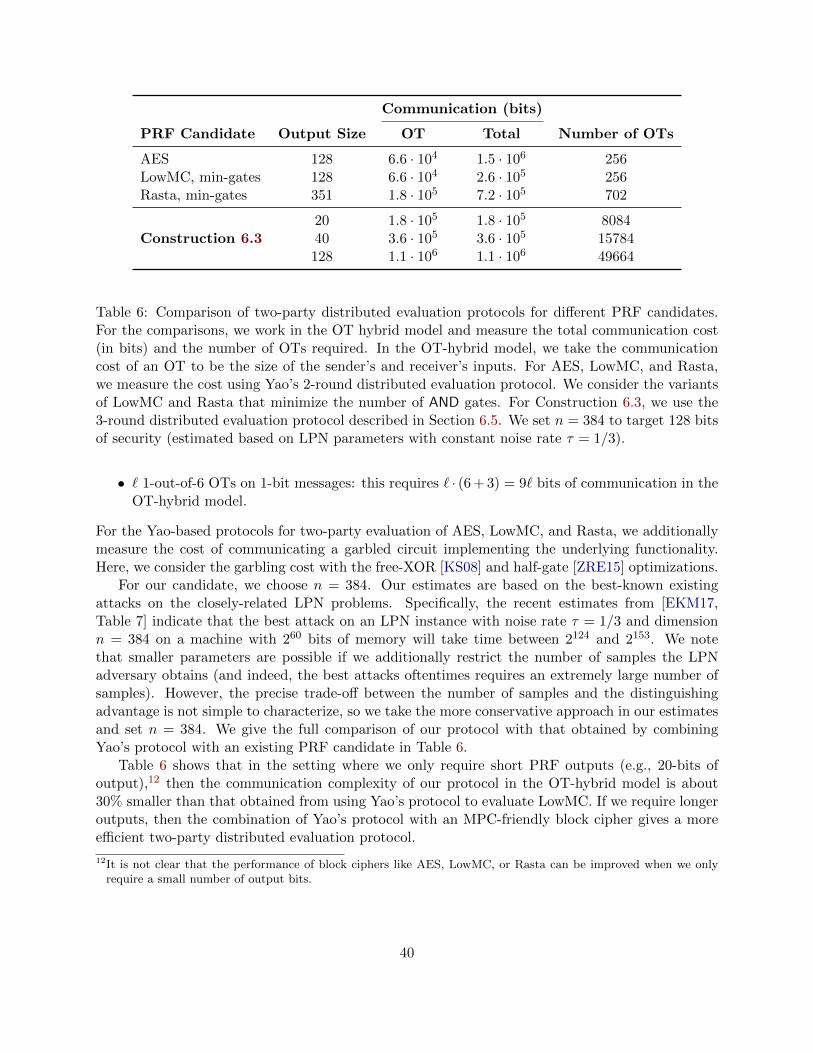
Communication (bits)

PRF Candidate Output Size OT Total Number of OTs

AES 128 6.6 · 104 1.5 · 106 256LowMC, min-gates 128 6.6 · 104 2.6 · 105 256Rasta, min-gates 351 1.8 · 105 7.2 · 105 702

Construction 6.320 1.8 · 105 1.8 · 105 808440 3.6 · 105 3.6 · 105 15784128 1.1 · 106 1.1 · 106 49664

Table 6: Comparison of two-party distributed evaluation protocols for different PRF candidates.For the comparisons, we work in the OT hybrid model and measure the total communication cost(in bits) and the number of OTs required. In the OT-hybrid model, we take the communicationcost of an OT to be the size of the sender’s and receiver’s inputs. For AES, LowMC, and Rasta,we measure the cost using Yao’s 2-round distributed evaluation protocol. We consider the variantsof LowMC and Rasta that minimize the number of AND gates. For Construction 6.3, we use the3-round distributed evaluation protocol described in Section 6.5. We set n = 384 to target 128 bitsof security (estimated based on LPN parameters with constant noise rate τ = 1/3).

• ` 1-out-of-6 OTs on 1-bit messages: this requires ` · (6 + 3) = 9` bits of communication in theOT-hybrid model.

For the Yao-based protocols for two-party evaluation of AES, LowMC, and Rasta, we additionallymeasure the cost of communicating a garbled circuit implementing the underlying functionality.Here, we consider the garbling cost with the free-XOR [KS08] and half-gate [ZRE15] optimizations.

For our candidate, we choose n = 384. Our estimates are based on the best-known existingattacks on the closely-related LPN problems. Specifically, the recent estimates from [EKM17,Table 7] indicate that the best attack on an LPN instance with noise rate τ = 1/3 and dimensionn = 384 on a machine with 260 bits of memory will take time between 2124 and 2153. We notethat smaller parameters are possible if we additionally restrict the number of samples the LPNadversary obtains (and indeed, the best attacks oftentimes requires an extremely large number ofsamples). However, the precise trade-off between the number of samples and the distinguishingadvantage is not simple to characterize, so we take the more conservative approach in our estimatesand set n = 384. We give the full comparison of our protocol with that obtained by combiningYao’s protocol with an existing PRF candidate in Table 6.

Table 6 shows that in the setting where we only require short PRF outputs (e.g., 20-bits ofoutput),12 then the communication complexity of our protocol in the OT-hybrid model is about30% smaller than that obtained from using Yao’s protocol to evaluate LowMC. If we require longeroutputs, then the combination of Yao’s protocol with an MPC-friendly block cipher gives a moreefficient two-party distributed evaluation protocol.

12It is not clear that the performance of block ciphers like AES, LowMC, or Rasta can be improved when we onlyrequire a small number of output bits.

40

6.6 Applications to Searchable Encryption

In this section, we describe how our shared-input shared-output oblivious PRF primitive can beused to build a distributed searchable symmetric encryption (SSE) system.

Distributed SSE. In the classic SSE problem [SWP00, Goh03, CGKO06], a single server holdsa set of encrypted documents and a client wants to retrieve all of the documents that match itsquery. Here, we focus on keyword search and we assume that each document is tagged with a setof keywords. A straightforward PRF-based SSE protocol works as follows. First, the client choosesa key k for a PRF F. Then, for each keyword w, the client adds a mapping from F(k,w) ontoan encrypted list of document indices (corresponding to the documents that contain the keywordw). To search, for a keyword w, the client who holds the PRF key computes the value F(k,w) andsends it to the server, which then looks up the value in the encrypted index and replies with theset of encrypted document indices. Security of the PRF ensures that the index does not reveal theset of keywords to the server. Note that if we work in the random oracle model, then even a weakPRF suffices to argue security. Namely, the tag associated with a keyword is F(k,H(w)), where Hhere is a hash function (modeled as a random oracle).

A limitation of the basic single-server SSE is that only clients who possess the secret PRF key kis able to search the database. In the distributed-SSE setting, a database curator can construct theindex (exactly as in the single-server SSE setting), but then secret share the PRF key to multipledifferent servers. When a client (who may be different from the database curator and who does notknow k) wants to perform a query on a keyword w, they would engage in an MPC protocol with theservers such that at the end of the protocol, the client learns F(k,H(w)) (and nothing more) whilethe servers learn nothing (about the query w). A shared-input, shared-key oblivious PRF directlyprovides an efficient solution for implementing distributed SSE. To query on a keyword w, an honestclient would first secret-share its input H(w) and send one share to each server. The servers wouldthen engage in an oblivious PRF evaluation where each server’s input is their individual key-shareand the share of the client’s query. At the end of the computation, the servers send the shares ofthe output F(k,H(w)) to the client, who reconstructs the shares and learns the tag F(k,H(w)).Now, the client can simply look up the entries associated with this tag in the database. Thus, ournew weak PRF candidate provides an efficient way of realizing distributed SSE assuming the clientis semi-honest. (If a client was malicious, it could query the weak PRF on arbitrary inputs of itschoosing; to achieve security in this setting, we will need to rely on the encoded-input weak PRFwe introduce in Section 7).

7 Encoded-Input Pseudorandom Functions

Motivated by applications in which a weak PRF does not suffice, in this section we introduce a new“encoded-input PRF” primitive that allows us to combine the efficiency advantages of weak PRFswith the security advantages of strong PRFs. Our candidate instantiations of this new primitivealso imply a depth-3 strong PRF variant of our main depth-2 weak PRF candidate.

As we showed in Section 5.3, there is already a non-adaptive attack against our basic weak PRFcandidate via sparse polynomial interpolation. In Appendix B, we show an even stronger result:namely, that strong PRFs do not exist in a large class of depth-2 circuits (which in particular alsoincludes the mod-p/mod-q generalizations of our candidate). Our lower bound relies on the classic

41

learning algorithm for automata with multiplicity by Bergadano and Varricchio [BV96].There are many scenarios where a weak PRF does not suffice for security. For instance, if we

consider the distributed SSE from Section 6.6 and impose the additional requirements of securityagainst malicious adversaries, then a weak PRF no longer suffices. To address this limitation,we introduce a new notion we call an encoded-input pseudorandom function (EI-PRF) that canbe used as a drop-in replacement for strong PRFs in many applications. At a high-level, an EI-PRF is a function that behaves like a PRF on some (possibly sparse) subset of the domain. As aconcrete example, a suitable subset might be the set of codewords under a linear error-correctingcode (Construction 7.9).

We now formally define the EI-PRF primitive, describe several natural applications, and proposecandidate instantiations whose efficiency is comparable to that of our weak PRF candidate. ThisEI-PRF candidate remains MPC-friendly, and can thus be useful for MPC applications that requirea strong PRF.

7.1 Definitions of (P)EI-PRFs

We define two versions of our notion: encoded-input pseudorandom function (EI-PRF) and protectedencoded-input pseudorandom function (PEI-PRF).

Definition 7.1 (Encoded-Input PRF). Let K = Kλλ∈N, X = Xλλ∈N, X ′ = X ′λλ∈N, and Y =Yλλ∈N be ensembles of finite sets indexed by a security parameter λ. Let F′λλ∈N = (Eλ,Fλ)λ∈Nbe an efficiently-computable collection of functions where Eλ : X ′λ → Xλ is an encoding functionand Fλ : Kλ × Xλ → Yλ is a keyed evaluation function. Then, we say that F′λλ∈N is a (t, ε)-encoded-input PRF (EI-PRF) if the function Kλ × X ′λ → Yλ defined via (k, x′) 7→ Fλ(k,Eλ(x′))is a (t, ε)-strong pseudorandom function. Moreover, we say that F′λ is computable in C if Fλ iscomputable in C.

While the definition of an encoded-input PRF may seem equivalent to that of a standard PRF,the important point is that the encoding function is a keyless procedure. This means that an honestuser can evaluate for itself the encoding algorithm on an input to obtain a valid encoded input, andthen ask for the PRF value on the encoded input. The holder of the PRF secret key only needsto evaluate F. This is the reason we define the complexity of an EI-PRF to be the complexityof its evaluation function (rather than the composition of its evaluation and encoding functions).Furthermore, we note that even though the overall function F(·,E(·)) is a strong PRF, the functionF itself may live in a complexity class where strong PRFs do not exist.

One of the main reasons we are interested in EI-PRFs is that we can potentially use them as adrop-in replacement for strong PRFs in concrete applications. In many of these scenarios, however,it does not make sense to assume that the evaluator behaves honestly and will only evaluate the Fon properly-encoded inputs. This motivates our stronger notion of a protected encoded-input PRF(PEI-PRF), which augments an EI-PRF with an additional verification algorithm. The inputs to aPEI-PRF consists of a point x as well as a proof w that x is a proper encoding (with respect to theencoding function of the underlying EI-PRF). The guarantee is that the output of the PEI-PRFare pseudorandom on all properly-encoded inputs, and ⊥ on improperly-encoded inputs.

Definition 7.2 (Protected EI-PRF). Let F′λλ∈N = (Eλ,Vλ,Fλ)λ∈N be an efficiently-computablecollection of functions where Eλ : X ′λ → Xλ ×Wλ is a protected encoding function whose range ispolynomial-time checkable by Vλ : Xλ ×Wλ → 0, 1. That is, Vλ(x,w) = 1 if and only if (x,w) is

42

a valid encoding. Finally, Fλ : Kλ × Xλ ×Wλ → Yλ is a keyed evaluation function. Denote by ⊥ aspecial element of Yλ. For a function f ∈ Funs[Xλ,Yλ], define Evalfλ : Xλ ×Wλ → Yλ as:

Evalfλ(x,w) =

f(x) if Vλ(x,w) = 1

⊥ otherwise.

Then, we say that F′λλ∈N is a (t, ε)-PEI-PRF if for all adversaries A running in time t(λ), and

taking kr←− Kλ and f

r←− Funs[Xλ,Yλ], we have that∣∣∣Pr[AFλ(k,·,·)(1λ) = 1]− Pr[AEvalfλ(·,·)(1λ) = 1]∣∣∣ ≤ ε(λ).

We say that F′λ is computable in a circuit class C if the mapping (k, x, w) 7→ Fλ(k, x, w) is computablein C. Finally, we say that a PEI-PRF is systematic if the witness w has the form x′‖w′ such thatVλ(x, (x′‖w′)) = 1 if and only if (x,w) = Eλ(x′).

Remark 7.3 (Relation between EI-PRFs and PEI-PRFs). PEI-PRFs are stronger objects thanEI-PRFs, since if (E,V,F) is a PEI-PRF, then (E,F) is an EI-PRF.

We first show that that PEI-PRFs can be generically constructed from EI-PRFs.

Lemma 7.4 (PEI-PRFs from EI-PRFs). Let (E∗λ,F∗λ)λ be an EI-PRF. Then, assuming Fλ andCNF formulas can be computed by depth-d circuits in a class C, there exists a systematic PEI-PRF(Eλ,Vλ,Fλ)λ computable by a depth-(d+ 1) circuit.

Proof. The lemma follows from the fact that we can check the correctness of any Boolean circuitcomputation using a CNF formula. In particular, we define a variable associated with each wire inthe circuit, and construct a constant-size CNF associated with each gate in the circuit (checkingthat the gate is implemented correctly). The conjunction of all of these gate-by-gate CNFs gives aCNF for the overall circuit. For notational convenience, we drop the λ subscripts in the descriptionbelow. We now define a systematic PEI-PRF (Eλ,Vλ,Fλ) as follows:

• E(x′)→ (x,w): On input a point x′ ∈ X ′, output (E∗(x′), w), where w is the set of all of thewire values for the Boolean circuit computing E∗(x′). Specifically, we can write w = x′‖w′,where x′ is the input to E∗ and w′ contain the internal (and output) wire values of E∗(x′).

• V(x,w) → 0, 1: On input an encoded input x ∈ X and a witness w ∈ W, the verificationalgorithm interprets w = x′‖w′. Then, it invokes the CNF verification procedure (for checkingcorrect computation of E∗) to check that E∗(x′) = (x,w).

• F(k, x, w) → y: On input the key k ∈ K, an encoded input x ∈ X , and a witness w ∈ W,the evaluation algorithm outputs y ← F∗(k, x) if V (x,w) = 1, and ⊥ otherwise. This can beimplemented by computing an AND between the output of V(x,w) and F∗(k, x).

Since the verification algorithm V can be expressed as a CNF formula, and moreover, both F∗ andCNFs can be computed by a circuit of depth d > 2, the evaluation algorithm F can be implementedby a circuit of depth d+ 1.

43

7.2 Applications of (P)EI-PRFs

We now describe several interesting applications of strong PRFs that can be based on PEI-PRFs.Certainly, we can instantiate any application of strong PRFs using an EI-PRF, since EI-PRFs arePRFs if we consider the combination of the encoding and the evaluation functions. However, wenote here that our notions of EI-PRFs and PEI-PRFs allow us to obtain interesting alternativeinstantiations of many of the classic applications of PRFs.

Symmetric encryption with low-depth decryption. A symmetric encryption scheme is atuple (G,E,D) such that the key-generation algorithm G(1λ) outputs a secret key k, the encryptionalgorithm E(k,m) outputs an encryption c of a message m, and the decryption algorithm D(k, c)outputs a string y such that D(k,E(k,m)) = m for all k,m. CPA-security of an encryption schemerequires that an efficient adversary given access to an encryption oracle E(k, ·) cannot distinguish anencryption of m0 from an encryption of m1 (for any two adversarially-chosen messages m0 and m1).The following theorem states how we can obtain a symmetric encryption scheme with low-depthdecryption from any EI-PRF.

Theorem 7.5 (Symmetric Encryption with Low-Depth Decryption). Let C be a circuit class.Then, if there exists an EI-PRF computable in C, there exists a symmetric encryption scheme withdecryption in C (assuming C is closed under composition with binary XOR gates).

Proof. This theorem follows direction from the textbook construction of symmetric encryption fromweak PRFs. Let (E∗,F∗) be an EI-PRF with key-space K, domain X ′, encoded domain X , andrange 0, 1. Then, we define our symmetric encryption scheme (G,E,D) over a binary messagespace M = 0, 1 as:

• G(1λ)→ k: On input the security parameter λ, sample and output an EI-PRF key kr←− K.

• E(k,m)→ (x, c): On input an EI-PRF key k ∈ K and a message m ∈ 0, 1, sample rr←− X ′

and output (E∗(r),m⊕ F∗(k,E∗(r))).

• D(k, (x, c)) → m: On input an EI-PRF key k ∈ K and a ciphertext (x, c), output m =c⊕ F∗(k, x).

Correctness and CPA-security are immediate by definition.

Remark 7.6 (Low-Complexity Symmetric Encryption). An important property of the constructionin Theorem 7.5 is that the decryption function does not need to evaluate the encoding function(since the ciphertext contains the encoded nonce x = E∗(x′)). Thus, assuming an EI-PRF in AC0

d

(resp., ACC0d), we obtain a symmetric encryption scheme where decryption can be implemented by

an AC0d+3 (resp., ACC0

d+1) circuit.13

MAC with low-depth verification. A MAC is a tuple (G,S,V) where the key-generationalgorithm G(1λ) outputs a secret key k, the signing algorithm S(k,m) outputs a MAC t of themessage m, and the verification algorithm V(k, (m, t)) outputs 1 if and only if t is a valid MACon m. Unforgeability requires that an efficient adversary with access to the signing oracle S(k, ·)cannot produce a MAC (on any message m) that was not previously output by the signing oracle.

13Fan-in 2 XOR gates can be computed by a depth-3 AC0 circuit and by a depth-1 ACC0 circuit.

44

MACs are immediate from strong PRFs: let G(1λ) outputs a PRF key k and define S(k,m) =F(k,m). Then V(k, (m, t)) simply checks if t = F(k,m). Security is immediate as any adversarythat can forge a MAC can also predict the output of the PRF on a previously-unqueried input.In fact, for this basic construction, an unpredictable function suffices, so plausibly, we can realizeMACs from weaker complexity classes (where strong PRFs may not exist). However, similar to thecase for PRFs, the existence of a learning algorithm for a class C also rules out the existence of anunpredictable function. Here we show that systematic PEI-PRFs are powerful enough for buildingMAC. In particular, we obtain the following theorem.

Theorem 7.7 (MACs with Low-Depth Verification). Let C be a circuit class. Then, if there existsa systematic PEI-PRF in C, there exists a MAC with verification in C (assuming C is closed undercomposition with an equality testing circuit).

Proof. Let F′ = (E,V′,F) be a systematic PEI-PRF with key-space K, domain X ′, encoded-domainX , witness space W, and range Y. We construct a MAC with message-space X ′ as follows:

• G(1λ) → k: On input the security parameter λ, the key-generation algorithm samples and

outputs a PEI-PRF key kr←− K.

• S(k,m) → (x,w, t): On input the signing key K ∈ K and a message m ∈ X ′, the signingalgorithm computes the encoding (x,w) = E(m) and the tag t = F(k, (x,w)). Finally, itoutputs (x,w, t).

• V(k,m, (x,w, t))→ 0, 1: On input the signing key k, the message m, and a tag (x,w, t), theverification algorithm outputs 1 if t = F(k, (x,w)) and that w = (m‖w′) for some bit-stringw′. Otherwise, the verification algorithm outputs 0.

Correctness and security immediately follows from the definition of systematic PEI-PRFs, andverification only relies on evaluating F and checking for equality.

Remark 7.8 (On Non-Systematic PEI-PRFs). Note that we require the PEI-PRF to be systematic,since the verification algorithm needs to check that (x,w) is a valid encoding of the target-messagem (as opposed to just a valid encoding of some message) without recomputing the encoding of m(which need not be a low-depth computation). We note that we can obtain a relaxed version of aMAC with low-depth verification from a non-systematic PEI-PRF if we instead define the messagespace to be the set of valid PEI-PRF encoded inputs (i.e. pairs (x,w) where V′(x,w) = 1).

CCA-secure symmetric encryption with low-depth decryption. Combining our CPA-secure encryption scheme with low-depth decryption (Theorem 7.5) and our MAC with low-depthverification (Theorem 7.7) yields a CCA-secure symmetric encryption scheme (in fact, an authenti-cated encryption scheme) with low-depth decryption via the classic “encrypt-then-MAC” construc-tion [BN00]. The decryption procedure of the resulting encryption scheme consists of evaluating thedecryption operation of the underlying scheme together with the MAC verification. This increasesthe depth of the overall decryption circuit by 1.

45

Distributed SSE for malicious clients. One of our primary motivations for introducing ourPEI-PRF notion is to realize a malicious-secure variant of our distributed SSE application. Specif-ically, in a distributed SSE application, a malicious client might issue queries that are invalid (i.e.,do not correspond to the output of the random oracle). In particular, a cheating client can learnthe outputs of the PRF on adaptively-chosen inputs, thereby compromising security. However, ifwe used a PEI-PRF, we can ensure the servers abort whenever the client tries to evaluate the PRFon an invalid input. This is done as follows: in addition to sending the servers a secret sharing of itsinput, it also sends the servers a secret sharing of the proof that its input is properly encoded. Theservers can then jointly evaluates the PEI-PRF. This ensures that the client will learn the outputof the PRF only if the client provided a valid encoding; otherwise, the client learns nothing.

7.3 Candidate Constructions of (P)EI-PRFs and Strong PRFs

We begin with a heuristic construction of PEI-PRFs from weak-PRFs using random oracles. Thisconstruction is primarily of conceptual interest and follows some basic observations on the connec-tion between weak and strong PRFs [NR95]. We then propose a candidate PEI-PRF based on ourmod-2/mod-3 weak PRF candidate (Construction 3.1) that remains MPC-friendly.

A heuristic approach to boost weak PRFs to PEI-PRFs. Suppose that F is a weak PRF.Then, the pair (H,F) is an EI-PRF, where the hash function H is modeled as a random oracle.Of course, this is a purely heuristic construction, since we cannot represent a random oracle (overa super-polynomial-size domain) by a polynomial-size circuit. However, we could heuristicallyinstantiate the random oracle by a concrete hash function like SHA-3. Then, the pair (SHA-3,F)gives a heuristic construction of an EI-PRF. This means that if F is a weak PRF computable bya depth-d circuit in a class C satisfying the requirements of Lemma 7.4, we obtain a heuristicconstruction of a PEI-PRF computable by a depth-(d+ 1) circuit in C. This in turn gives heuristicconstructions of the applications from Section 7.2 (to symmetric encryption and MACs).

(P)EI-PRF from our candidate. Next, we propose a candidate PEI-PRF based on Construc-tion 3.1 whose design is well-suited for our MPC applications. In particular, we need an encodingfunction such that the outputs of the PRF on all encoded inputs appear pseudorandom. At a highlevel, both the non-adaptive attack (Section 5.3) and the adaptive attack (Appendix B) on ourweak PRF candidate relies on querying inputs that are heavily correlated (e.g., have low Hammingdistance). This suggests that using a code with large minimal distance to encode the input x shouldprevent these attacks. For MPC-friendliness, we would like to use a linear code, as verifying thatan input is a valid codeword can be done efficiently (by multiplying by the parity-check matrix forthe code).

A natural candidate is to use a linear code (G,H) over Z2: the encoding of an input x′ is thecodeword G · x′. Unfortunately, the same attack still applies since we can always view the PRFevaluation as A · (G · x′) = (A ·G) · x′ and interpret (A ·G) as the key. To defend against this, weinstead use a linear code over Z3 and define the encoded bitstring x to be the binary representationof the codeword obtained by applying the code to x′ (where we interpret x′ ∈ 0, 1n′ as a vectorover Z3). By mixing mod-2 and mod-3 operations, the encoding procedure becomes non-linear,but verification can still be expressed as a linear function. At the same time, the use of the linearcode ensures that (1) encoded inputs are far from each other, (2) verification is MPC-friendly

46

as the code is linear, and (3) the input of the second mapping cannot be expressed as a read-once computation (this property is important for resisting the learning automata with multiplicityattacks from [BV96]).

Construction 7.9 (EI-PRF and PEI-PRF Candidate). Let λ be a security parameter, and taken = n(λ), n′ = n′(λ), and m = m(λ). Let G ∈ Zn

′×n3 and H ∈ Zn

′−n×n′3 be the generator and

parity-check matrices, respectively, for a linear error-correcting code over Z3. We use G and H toconstruct a candidate EI-PRF (Eλ,Fλ) and PEI-PRF (Eλ,Vλ,Fλ) with domain 0, 1n and rangeZ3 as follows:

• EI-PRF: We define the encoding function Eλ : 0, 1n → 0, 12n′ for our encoded-input PRFto be the mapping x′ ∈ 0, 1n 7→ bin(G·x′) ∈ 0, 12n′ , where bin is a “binary decomposition”operator. In words, the encoding function Eλ takes as input an element in 0, 1n, interprets itas a binary-valued vector in Zn3 , maps it to a codeword w ∈ Zn′3 , and then outputs the binaryrepresentation of the elements of w. Namely, each element of w is a Z3 element which we canencode using two bits. Next, we take Fλ : Zm×2n′

2 ×Z2n′2 → Z3 to be our weak PRF candidate

(Construction 3.1) with input length 2n′. The encoded-input PRF is the pair (Eλ,Fλ).

• PEI-PRF: Our candidate PEI-PRF construction is defined as (Eλ,Vλ,Fλ) where Eλ and Fλare defined as above (for our EI-PRF candidate). Checking that an input is properly encodedis now possible using the parity-check matrix (the input is the encoded codeword and thewitness is empty). In particular, on input an encoded input x ∈ 0, 12n′ , the verificationalgorithm Vλ : 0, 12n′ → 0, 1 outputs 1 if (H · B · x = 0n

′−n) and 0 otherwise, whereB ∈ Zn

′×2n′

3 denotes the powers-of-two matrix:

B = (2 1)⊗ In′ =

2 1 0 · · · 00 0 2 1 0 · · · 0

. . .

0 · · · 0 2 1

,

where In′ denotes the (n′ × n′) identity matrix. By construction, on input a binary vectorx ∈ 0, 12n′ , the mapping Bx returns the unique y ∈ Zn′3 such x = bin(y).

Note that we can obtain a systematic PEI-PRF by assuming that G has the form (Ik|P)T sothat it transforms an input x′ into a codeword of the form (x′,P · x′). This is without loss ofgenerality.

Remark 7.10 (Non-Interactive Verification). The verification algorithm for our PEI-PRF can-didate in Construction 7.9 is a linear function over Z3. Thus, there is an efficient distributedprotocol where multiple servers, who each hold a linear secret-sharing of the encoded input, cannon-interactively compute a share of the verification bit for their shared input.

Remark 7.11 (Fully-Distributed Evaluation). We can easily extend our 3-party protocol for eval-uating our weak PRF candidate (Construction 3.1) to obtain a similar protocol for distributedevaluation of our PEI-PRF candidate in Construction 7.9. In this setting, our objective is to de-fend against a malicious client. The servers are still assumed to be semi-honest. The only additionalcomponent we require is a way for the servers the check that the input is valid before releasing theshares of the output. One possibility is to have the client provide secret shares of the encoded input

47

over both Z2 and Z3 to the servers. The servers would use the Z2-secret shares to evaluate thePRF (using the distributed evaluation protocol from Figure 2) and the Z3-secret shares to verifythe encodings (using the approach from Remark 7.10).

Unfortunately, a malicious client can provide inconsistent shares. Instead, we only require theclient to submit a Z2-sharing of the encoded input and have the servers use the share-conversionprotocol π2,3 (Definition 6.2, Figure 1) to convert this sharing into a Z3-sharing (between 2 out of the3 servers). The two servers can then non-interactively compute a secret sharing of the verificationbit (since the verification algorithm is linear). Naıvely, performing the verification check introducesan additional round in the evaluation protocol since we need the servers to reveal the verificationbit before publishing their shares of the output. Fortunately, in the share-conversion protocol π2,3,one of the two servers that obtains a share of the Z3-sharing picks its share. This means that thisserver can output its share of the verification in the first round and its share of the PRF outputin the second round. The other server then computes its share of the verification bit after thefirst round, checks if the verification is successful, and outputs its share of the PRF output only ifthe verification is successful. Otherwise, it does not output anything. This ensures that the clientdoes not learn anything about the PRF value if the input is not properly encoded, thus yielding a2-round distributed SSE protocol with security against a malicious client.

Instantiating Construction 7.9. Our main conjecture is that instantiating Construction 7.9with a random linear code yields an (exponentially-secure) encoded-input PRF. We state our mainconjecture below, and then describe several variants:

Conjecture 7.12 (Exponential Hardness of Encoded-Input PRF Candidate). Let λ be a securityparameter. Then, there exist constants c1, c2, c3, c4 > 0 such that for n = c1λ, n′ = c2λ, m = c3λand t = 2λ, the function family (Eλ,Fλ)λ∈N from Construction 7.9, when instantiated using a

random linear code (i.e., sample a uniformly random generator matrix Gr←− Zn

′×n3 and publish G

as part of the description of the EI-PRF), is a (t, ε)-EI-PRF for ε = 2−c4λ. Correspondingly, forthis choice of linear code, the function family (Eλ,Vλ,Fλ)λ∈N is a (t, ε)-PEI-PRF.

We leave the question of further evaluating the conjecture and studying the concrete achievabletradeoffs between the parameters c1, c2, c3, c4 for further study.

Remark 7.13 (Alternative Instantiations of Construction 7.9). We now describe several alternativeinstantiations of Construction 7.9 and its associated hardness conjecture (Conjecture 7.12):

• Using a specific linear code: Instead of using a random linear code for the encoding func-tion, we can formulate Construction 7.9 (and Conjecture 7.12) for a specific choice (or family)of linear codes. For example, in our application to natural proof barriers (Remark 7.15), werely on an instantiation using the Druk-Ishai [DI14] family of codes.

• A simpler encoding function. Instead of taking the binary decomposition of the mod-3codeword in the encoding function Eλ, we can define a simpler encoding function Eλ : 0, 1n →0, 1n′ to be the mapping x′ 7→ lsb(G · x′), where lsb returns the least significant bit of eachmod-3 component of the codeword G · x′ ∈ Zn′3 . This encoding function has the advantagethat it preserves the length of the codeword. A drawback of this encoding function is thatverification is no longer a linear function (unlike bin, the lsb function is not even invertible).This makes it less suitable for distributed evaluation (Remarks 7.10 and 7.11).

48

Remark 7.14 (Candidate Strong PRF in Depth-3 ACC0[2, 3]). Construction 7.9 gives a strongPRF candidate if we consider the composition of the encoding function E with the evaluationfunction F. The strong PRF candidate starts by applying a public mod-3 linear encoding functionto the input, then interprets the result as a vector over Z2 and applies a secret random mod-2linear mapping, and finally interprets the result as a vector over Z3 and outputs the sum of itsentries. (One could obtain a variant with a longer output by using a suitable compressive mod-3linear mapping for the final step, as in our weak PRF candidate.) Since the encoding function Ecomputes a linear function over Z3, it can be computed by a depth-1 ACC0[3] circuit. As notedin Remark 3.10, the PRF evaluation function F can be computed by a depth-2 ACC0[2, 3] circuit.Thus, the composition of E and F can be computed by a depth-3 ACC0 circuit (note that the binarydecomposition in the encoding function is easily handled via fan-in and does not increase the depthof the circuit). More precisely, under Conjecture 7.12, we obtain a strong PRF with exponentialsecurity in depth-3 ACC0[2, 3] by instantiating the error-correcting code in Construction 7.9 witha random linear code. One could also consider a seemingly more conservative variant where themod-3 linear encoding function is secret.

Remark 7.15 (Asymptotically-Optimal Strong PRFs and Natural Proof Barriers). As noted inRemark 7.14, Construction 7.9 gives a strong PRF candidate if we consider the composition of theencoding function E with the evaluation function F. If both E and F can be computed by a circuit ofsize O(λ) (where all parameters are linear in λ, as in Conjecture 7.12), then we obtain a candidatestrong PRF with exponential security that can be computed by linear-size circuits. This gives an“asymptotically optimal” PRF that rules out natural proofs of super-linear circuit lower boundsin the sense of Razborov and Rudich [RR94]. We now describe a variant of our EI-PRF fromConstruction 7.9 that gives the first candidate instantiation of an asymptotically-optimal PRF,and correspondingly, the first natural proof barrier for proving super-linear circuit lower bounds.

Evaluating our EI-PRF candidate from Construction 7.9 consists of three main steps: encodingthe input over Z3, computing the binary decomposition of the encoded vector, and then multiplyingthe encoded input with the secret key A over Z2. If we instantiate the Z3-encoding with a linear-time encodable code over Z3 and then replace the key A with the generator matrix of a linear-timeencodable code over Z2, then the resulting construction can be computed by a linear-size circuit.For instance, we can instantiate the code with the linear-time encodable code family proposedby Druk and Ishai [DI14] (which builds on the hash function from [IKOS08]). This family givesa randomized construction of a linear-time encodable code that has many of the combinatorialproperties of a random linear code. Thus, we conjecture that sampling the key to be the generatormatrix of a Druk-Ishai code does not compromise the security of our candidate. Putting thesepieces together, we obtain a plausible candidate of a strong PRF with exponential security andwhich can be computed by a linear-size circuit. As far as we know, this is the first candidateinstantiation of such an asymptotically-optimal strong PRF. Assuming it is indeed exponentiallysecure, natural proof techniques cannot prove super-linear circuit lower bounds.

Conclusions. We believe that the conjectures we have made in this section are strong and ahealthy dose of skepticism is warranted. We hope that the applications and implications we pointout will motivate further study and constructions of (P)EI-PRFs, as well as additional cryptanalysisof our concrete candidates. We also leave open the question of setting concrete parameters for ournew PEI-PRF (Construction 7.9) and strong PRF candidates (Remark 7.14 and Conjecture 7.12).

49

Acknowledgments

We thank Benny Applebaum, Andrej Bogdanov, Arkadev Chattopadhyay, Itai Dinur, Neeraj Kayal,Sam Kim, Hart Montgomery, Alon Rosen, Adi Shamir, Alexander Sherstov, Nitzan Tur, EmanueleViola, Gilles Zemor, and the anonymous TCC reviewers for helpful discussions and pointers.D. Boneh and D. J. Wu were supported by NSF, DARPA, a grant from ONR, and the SimonsFoundation. Y. Ishai, A. Passelegue, and A. Sahai were supported in part from a DARPA/ARLSAFEWARE award, NSF Frontier Award 1413955, NSF grants 1619348, 1228984, 1136174, and1065276, BSF grant 2012378, NSF-BSF grant 2015782, a Xerox Faculty Research Award, a GoogleFaculty Research Award, an equipment grant from Intel, and an Okawa Foundation Research Grant.Y. Ishai was additionally supported by ERC grant 742754, ISF grant 1709/14, and a grant from theMinistry of Science and Technology, Israel and Department of Science and Technology, Governmentof India. This material is based upon work supported by the Defense Advanced Research ProjectsAgency through the ARL under Contract W911NF-15-C-0205. The views expressed are those ofthe authors and do not reflect the official policy or position of the Department of Defense, theNational Science Foundation, or the U.S. Government.

References

[ABB+17] Nicolas Aragon, Paulo Barreto, Slim Bettaieb, Loıc Bidoux, Olivier Blazy, Jean-Christophe Deneuville, Philippe Gaborit, Shay Gueron, Tim Guneysu, Carlos AguilarMelchor, et al. BIKE: Bit flipping key encapsulation. 2017.

[ABG+14] Adi Akavia, Andrej Bogdanov, Siyao Guo, Akshay Kamath, and Alon Rosen. Candi-date weak pseudorandom functions in AC0 o MOD2. In ITCS 2014, pages 251–260,2014.

[ACPS09] Benny Applebaum, David Cash, Chris Peikert, and Amit Sahai. Fast crypto-graphic primitives and circular-secure encryption based on hard learning problems.In CRYPTO, pages 595–618, 2009.

[AFL+16] Toshinori Araki, Jun Furukawa, Yehuda Lindell, Ariel Nof, and Kazuma Ohara. High-throughput semi-honest secure three-party computation with an honest majority. InACM CCS, pages 805–817, 2016.

[AG11] Sanjeev Arora and Rong Ge. New algorithms for learning in presence of errors. InICALP 2011ICALP, pages 403–415, 2011.

[AGR14] Andrew Arnold, Mark Giesbrecht, and Daniel S Roche. Sparse interpolation over finitefields via low-order roots of unity. In Proceedings of the 39th International Symposiumon Symbolic and Algebraic Computation, pages 27–34. ACM, 2014.

[AGR+16] Martin R. Albrecht, Lorenzo Grassi, Christian Rechberger, Arnab Roy, and TygeTiessen. MiMC: Efficient encryption and cryptographic hashing with minimal mul-tiplicative complexity. In ASIACRYPT 2016, pages 191–219, 2016.

[AIK04] Benny Applebaum, Yuval Ishai, and Eyal Kushilevitz. Cryptography in NC0. In FOCS,pages 166–175, 2004.

50

[AIK09] Benny Applebaum, Yuval Ishai, and Eyal Kushilevitz. Cryptography with constantinput locality. Journal of Cryptology, 22(4):429–469, October 2009.

[AIK11] Benny Applebaum, Yuval Ishai, and Eyal Kushilevitz. How to garble arithmetic cir-cuits. In FOCS, pages 120–129, 2011.

[AKK+03] Noga Alon, Tali Kaufman, Michael Krivelevich, Simon Litsyn, and Dana Ron. Testinglow-degree polynomials over GF(2). In APPROX-RANDOM, pages 188–199, 2003.

[AKPW13] Joel Alwen, Stephan Krenn, Krzysztof Pietrzak, and Daniel Wichs. Learning withrounding, revisited - new reduction, properties and applications. In CRYPTO, pages57–74, 2013.

[App13] Benny Applebaum. Cryptographic hardness of random local functions-survey. In TCC,page 599, 2013.

[AR16] Benny Applebaum and Pavel Raykov. Fast pseudorandom functions based on expandergraphs. In TCC 2016-BTCC, pages 27–56, 2016.

[ARS+15] Martin R. Albrecht, Christian Rechberger, Thomas Schneider, Tyge Tiessen, andMichael Zohner. Ciphers for MPC and FHE. In EUROCRYPT, pages 430–454, 2015.

[ASA16] Jacob Alperin-Sheriff and Daniel Apon. Dimension-preserving reductions from LWEto LWR. Cryptology ePrint Archive, Report 2016/589, 2016. http://eprint.iacr.

org/2016/589.

[Bar85] David A. Barrington. Width-3 permutation branching programs. Technical Memoran-dum TM-293, 1985.

[BCGI18] Elette Boyle, Geoffroy Couteau, Niv Gilboa, and Yuval Ishai. Compressing vectorOLE. In ACM CCS, pages 896–912, 2018.

[BDOZ11] Rikke Bendlin, Ivan Damgard, Claudio Orlandi, and Sarah Zakarias. Semi-homomorphic encryption and multiparty computation. In EUROCRYPT, pages 169–188, 2011.

[Bea92] Donald Beaver. Efficient multiparty protocols using circuit randomization. InCRYPTO, pages 420–432, 1992.

[Bea95] Donald Beaver. Precomputing oblivious transfer. In CRYPTO, pages 97–109, 1995.

[BFKL94] Avrim Blum, Merrick L. Furst, Michael J. Kearns, and Richard J. Lipton. Crypto-graphic primitives based on hard learning problems. In CRYPTO, pages 278–291,1994.

[BGM+16] Andrej Bogdanov, Siyao Guo, Daniel Masny, Silas Richelson, and Alon Rosen. Onthe hardness of learning with rounding over small modulus. In TCC 2016-A, pages209–224, 2016.

[BHR12] Mihir Bellare, Viet Tung Hoang, and Phillip Rogaway. Foundations of garbled circuits.In ACM CCS, pages 784–796, 2012.

51

[BIP+18] Dan Boneh, Yuval Ishai, Alain Passelegue, Amit Sahai, and David J. Wu. Exploringcrypto dark matter: New simple PRF candidates and their applications. In TCC, pages699–729, 2018.

[BKW00] Avrim Blum, Adam Kalai, and Hal Wasserman. Noise-tolerant learning, the parityproblem, and the statistical query model. In ACM STOC, pages 435–440, 2000.

[BLMR13] Dan Boneh, Kevin Lewi, Hart William Montgomery, and Ananth Raghunathan. Keyhomomorphic PRFs and their applications. In CRYPTO, pages 410–428, 2013.

[BN00] Mihir Bellare and Chanathip Namprempre. Authenticated encryption: Relationsamong notions and analysis of the generic composition paradigm. In ASIACRYPT,pages 531–545, 2000.

[BOGW88] Michael Ben-Or, Shafi Goldwasser, and Avi Wigderson. Completeness theorems fornon-cryptographic fault-tolerant distributed computation (extended abstract). In ACMSTOC, pages 1–10, 1988.

[BOT88] Michael Ben-Or and Prasoon Tiwari. A deterministic algorithm for sparse multivariatepolynominal interpolation (extended abstract). In ACM STOC, pages 301–309, 1988.

[BP14] Abhishek Banerjee and Chris Peikert. New and improved key-homomorphic pseudo-random functions. In CRYPTO, pages 353–370, 2014.

[BPR12] Abhishek Banerjee, Chris Peikert, and Alon Rosen. Pseudorandom functions and lat-tices. In EUROCRYPT, pages 719–737, 2012.

[BR17] Andrej Bogdanov and Alon Rosen. Pseudorandom functions: Three decades later. InYehuda Lindell, editor, Tutorials on the Foundations of Cryptography., pages 79–158.Springer International Publishing, 2017.

[BV96] Francesco Bergadano and Stefano Varricchio. Learning behaviors of automata frommultiplicity and equivalence queries. SIAM J. Comput., 25(6):1268–1280, 1996.

[Can06] Christophe De Canniere. Trivium: A stream cipher construction inspired by blockcipher design principles. In ISC 2006, pages 171–186, 2006.

[CCD88] David Chaum, Claude Crepeau, and Ivan Damgard. Multiparty unconditionally secureprotocols (extended abstract). In ACM STOC, pages 11–19, 1988.

[CCF+16] Anne Canteaut, Sergiu Carpov, Caroline Fontaine, Tancrede Lepoint, Marıa Naya-Plasencia, Pascal Paillier, and Renaud Sirdey. Stream ciphers: A practical solution forefficient homomorphic-ciphertext compression. In FSE, pages 313–333, 2016.

[CDI05] Ronald Cramer, Ivan Damgard, and Yuval Ishai. Share conversion, pseudorandomsecret-sharing and applications to secure computation. In TCC, pages 342–362, 2005.

[CGH+85] Benny Chor, Oded Goldreich, Johan Hastad, Joel Friedman, Steven Rudich, and Ro-man Smolensky. The bit extraction problem of t-resilient functions (preliminary ver-sion). In FOCS, pages 396–407, 1985.

52

[CGKO06] Reza Curtmola, Juan A. Garay, Seny Kamara, and Rafail Ostrovsky. Searchable sym-metric encryption: improved definitions and efficient constructions. In ACM CCS,pages 79–88, 2006.

[Cho16] Tung Chou. Sandy2x: New Curve25519 speed records. In SAC, pages 145–160, 2016.

[CIKK16] Marco L. Carmosino, Russell Impagliazzo, Valentine Kabanets, and AntoninaKolokolova. Learning algorithms from natural proofs. In CCC, pages 10:1–10:24,2016.

[DEG+18] Christoph Dobraunig, Maria Eichlseder, Lorenzo Grassi, Virginie Lallemand, GregorLeander, Eik List, Florian Mendel, and Christian Rechberger. Rasta: A cipher withlow ANDdepth and few ANDs per bit. In CRYPTO, pages 662–692, 2018.

[DGN+17] Nico Dottling, Satrajit Ghosh, Jesper Buus Nielsen, Tobias Nilges, and Roberto Tri-filetti. TinyOLE: Efficient actively secure two-party computation from oblivious linearfunction evaluation. In ACM CCS, pages 2263–2276, 2017.

[DI14] Erez Druk and Yuval Ishai. Linear-time encodable codes meeting the Gilbert-Varshamov bound and their cryptographic applications. In ITCS, pages 169–182, 2014.

[DLM+07] Ilias Diakonikolas, Homin K. Lee, Kevin Matulef, Krzysztof Onak, Ronitt Rubinfeld,Rocco A. Servedio, and Andrew Wan. Testing for concise representations. In FOCS,pages 549–558, 2007.

[DPSZ12] Ivan Damgard, Valerio Pastro, Nigel P. Smart, and Sarah Zakarias. Multiparty com-putation from somewhat homomorphic encryption. In CRYPTO, pages 643–662, 2012.

[EKM17] Andre Esser, Robert Kubler, and Alexander May. LPN decoded. In CRYPTO, pages486–514, 2017.

[EKR95] Funda Ergun, Ravi Kumar, and Ronitt Rubinfeld. On learning bounded-width branch-ing programs. In COLT, pages 361–368, 1995.

[FIPR05] Michael J. Freedman, Yuval Ishai, Benny Pinkas, and Omer Reingold. Keyword searchand oblivious pseudorandom functions. In TCC, pages 303–324, 2005.

[GGM84] Oded Goldreich, Shafi Goldwasser, and Silvio Micali. On the cryptographic applicationsof random functions. In CRYPTO, pages 276–288, 1984.

[GGM86] Oded Goldreich, Shafi Goldwasser, and Silvio Micali. How to construct random func-tions. Journal of the ACM, 33(4):792–807, October 1986.

[GMW87] Oded Goldreich, Silvio Micali, and Avi Wigderson. How to play any mental game orA completeness theorem for protocols with honest majority. In ACM STOC, pages218–229, 1987.

[Goh03] Eu-Jin Goh. Secure indexes. Cryptology ePrint Archive, Report 2003/216, 2003.http://eprint.iacr.org/2003/216.

53

[Gol00] Oded Goldreich. Candidate one-way functions based on expander graphs. CryptologyePrint Archive, Report 2000/063, 2000. http://eprint.iacr.org/2000/063.

[GRS08] Henri Gilbert, Matthew J. B. Robshaw, and Yannick Seurin. HB]: Increasing thesecurity and efficiency of HB+. In EUROCRYPT, pages 361–378, 2008.

[GS09] Sanchit Garg and Eric Schost. Interpolation of polynomials given by straight-lineprograms. Theoretical Computer Science, 410(27-29):2659–2662, 2009.

[HILL99] Johan Hastad, Russell Impagliazzo, Leonid A. Levin, and Michael Luby. A pseudoran-dom generator from any one-way function. SIAM Journal on Computing, 28(4):1364–1396, 1999.

[HKL+12] Stefan Heyse, Eike Kiltz, Vadim Lyubashevsky, Christof Paar, and Krzysztof Pietrzak.Lapin: An efficient authentication protocol based on ring-LPN. In FSE, pages 346–365,2012.

[IK00] Yuval Ishai and Eyal Kushilevitz. Randomizing polynomials: A new representationwith applications to round-efficient secure computation. In FOCS, pages 294–304,2000.

[IKM+13] Yuval Ishai, Eyal Kushilevitz, Sigurd Meldgaard, Claudio Orlandi, and Anat Paskin-Cherniavsky. On the power of correlated randomness in secure computation. In TCC,pages 600–620, 2013.

[IKOS08] Yuval Ishai, Eyal Kushilevitz, Rafail Ostrovsky, and Amit Sahai. Cryptography withconstant computational overhead. In ACM STOC, pages 433–442, 2008.

[IPS08] Yuval Ishai, Manoj Prabhakaran, and Amit Sahai. Founding cryptography on oblivioustransfer - efficiently. In CRYPTO, pages 572–591, 2008.

[IPS09] Yuval Ishai, Manoj Prabhakaran, and Amit Sahai. Secure arithmetic computation withno honest majority. In TCC, pages 294–314, 2009.

[JL09] Stanislaw Jarecki and Xiaomin Liu. Efficient oblivious pseudorandom function withapplications to adaptive OT and secure computation of set intersection. In TCC, pages577–594, 2009.

[JPRZ04] Charanjit S. Jutla, Anindya C. Patthak, Atri Rudra, and David Zuckerman. Testinglow-degree polynomials over prime fields. In FOCS, pages 423–432, 2004.

[Kha93] Michael Kharitonov. Cryptographic hardness of distribution-specific learning. In ACMSTOC, pages 372–381, 1993.

[Kil88] Joe Kilian. Founding cryptography on oblivious transfer. In ACM STOC, pages 20–31,1988.

[KL01] Matthias Krause and Stefan Lucks. Pseudorandom functions in TC0 and cryptographiclimitations to proving lower bounds. Computational Complexity, 10(4):297–313, 2001.

54

[KOS16] Marcel Keller, Emmanuela Orsini, and Peter Scholl. MASCOT: Faster malicious arith-metic secure computation with oblivious transfer. In ACM CCS, pages 830–842, 2016.

[KS08] Vladimir Kolesnikov and Thomas Schneider. Improved garbled circuit: Free XOR gatesand applications. In ICALP 2008, pages 486–498, 2008.

[KY88] Erich Kaltofen and Lakshman Yagati. Improved sparse multivariate polynomial inter-polation algorithms. In International Symposium on Symbolic and Algebraic Compu-tation, pages 467–474. Springer, 1988.

[LMN89] Nathan Linial, Yishay Mansour, and Noam Nisan. Constant depth circuits, fouriertransform, and learnability. In FOCS, pages 574–579, 1989.

[MBD+18] Carlos Aguilar Melchor, Olivier Blazy, Jean-Christophe Deneuville, Philippe Gaborit,and Gilles Zemor. Efficient encryption from random quasi-cyclic codes. IEEE Trans.Information Theory, 64(5):3927–3943, 2018.

[MJSC16] Pierrick Meaux, Anthony Journault, Francois-Xavier Standaert, and Claude Carlet.Towards stream ciphers for efficient FHE with low-noise ciphertexts. In EUROCRYPT,pages 311–343, 2016.

[MV12] Eric Miles and Emanuele Viola. Substitution-permutation networks, pseudorandomfunctions, and natural proofs. In CRYPTO, pages 68–85, 2012.

[NP99] Moni Naor and Benny Pinkas. Oblivious transfer and polynomial evaluation. In ACMSTOC, pages 245–254, 1999.

[NPR99] Moni Naor, Benny Pinkas, and Omer Reingold. Distributed pseudo-random functionsand KDCs. In EUROCRYPT, pages 327–346, 1999.

[NR95] Moni Naor and Omer Reingold. Synthesizers and their application to the parallelconstruction of pseudo-random functions. In FOCS, pages 170–181, 1995.

[NR99] Moni Naor and Omer Reingold. Synthesizers and their application to the parallelconstruction of pseudo-random functions. Journal of Computer and System Sciences,58(2):336–375, 1999.

[NR04] Moni Naor and Omer Reingold. Number-theoretic constructions of efficient pseudo-random functions. Journal of the ACM, 51(2):231–262, 2004.

[NRR00] Moni Naor, Omer Reingold, and Alon Rosen. Pseudo-random functions and factoring(extended abstract). In ACM STOC, pages 11–20, 2000.

[Pan15] Pavel Panteleev. Fast systematic encoding of quasi-cyclic codes using the chinese re-mainder theorem. In IEEE International Symposium on Information Theory, ISIT2015, Hong Kong, China, June 14-19, 2015, pages 1916–1920, 2015.

[Pie12] Krzysztof Pietrzak. Cryptography from learning parity with noise. In SOFSEM, pages99–114, 2012.

55

[PRS02] Michal Parnas, Dana Ron, and Alex Samorodnitsky. Testing basic boolean formulae.SIAM Journal on Discrete Mathematics, 16(1):20–46, 2002.

[Raz87] Alexander A. Razborov. Lower bounds on the size of bounded-depth networks over acomplete basis with logical addition (russian). Matematicheskie Zametki, 41(4):598–607, 1987. English translation in Mathematical Notes of the Academy of Sci. of theUSSR, 41(4):333-338, 1987.

[Reg05] Oded Regev. On lattices, learning with errors, random linear codes, and cryptography.In ACM STOC, pages 84–93, 2005.

[RR94] Alexander A. Razborov and Steven Rudich. Natural proofs. In ACM STOC, pages204–213, 1994.

[Sha08] Adi Shamir. SQUASH - a new MAC with provable security properties for highlyconstrained devices such as RFID tags. In FSE, pages 144–157, 2008.

[Sho94] Peter W. Shor. Algorithms for quantum computation: Discrete logarithms and factor-ing. In FOCS, pages 124–134, 1994.

[Smo87] Roman Smolensky. Algebraic methods in the theory of lower bounds for Boolean circuitcomplexity. In ACM STOC, pages 77–82, 1987.

[SWP00] Dawn Xiaodong Song, David Wagner, and Adrian Perrig. Practical techniques forsearches on encrypted data. In IEEE Symposium on Security and Privacy, pages 44–55, 2000.

[Val84] Leslie G. Valiant. A theory of the learnable. In ACM STOC, pages 436–445, 1984.

[Ver90] Karsten A. Verbeurgt. Learning DNF under the uniform distribution in quasi-polynomial time. In COLT, pages 314–326, 1990.

[Vio13] Emanuele Viola. The communication complexity of addition. In SODA, pages 632–651,2013.

[Wer94] Kai Werther. The complexity of sparse polynomial interpolation over finite fields.Applicable Algebra in Engineering, Communication and Computing, 5(2):91–103, 1994.

[Yao86] Andrew Chi-Chih Yao. How to generate and exchange secrets (extended abstract). InFOCS, pages 162–167, 1986.

[YS16] Yu Yu and John P. Steinberger. Pseudorandom functions in almost constant depthfrom low-noise LPN. In EUROCRYPT, pages 154–183, 2016.

[Zip79] Richard Zippel. Probabilistic algorithms for sparse polynomials. In EUROSAM, pages216–226, 1979.

[Zip90] Richard Zippel. Interpolating polynomials from their values. J. Symb. Comput.,9(3):375–403, 1990.

[ZRE15] Samee Zahur, Mike Rosulek, and David Evans. Two halves make a whole - reducingdata transfer in garbled circuits using half gates. In EUROCRYPT, pages 220–250,2015.

56

A Proofs from Section 4

In this section, we give the proofs from Section 4.

A.1 Proof of Lemma 4.1

We first prove the claim for the setting where the H contains a single function. The claim thenfollows by a union bound. Consider a function h : 0, 1n → 0,±1 and define the random variable

Z(A) = Prx [map(Ax) = h(x)] = Ex[1(map(Ax), h(x))],

where 1(x, y) is the indicator function: 1(x, y) = 1 if and only if x = y and 0 otherwise. Then, wehave

EA[Z(A)] = EA[Ex[1(map(Ax), h(x))]] = Ex[EA[1(map(Ax), h(x))]]

=1

2n·

1(0n, h(0n)) +∑x 6=0n

EA[1(map(Ax), h(x))]

For a uniformly random choice of A and x 6= 0n, we have that Ax is uniform and independent ofx. Hence, for any fixed x 6= 0n, we have:

EA[1(map(Ax), h(x))] = Ey[1(map(y), h(x))] = Pry [map(y) = h(x)] .

We next need to use the following claim about the distribution of the mapping.

Claim A.1. For any n > 0 and b ∈ 0,±1 and taking yr←− 0, 1n,∣∣∣∣Pr[map(y) = b]− 1

3

∣∣∣∣ ≤ 1

2n.

Proof. We show the following: for each n, the number of bitstring mapped to each of (0, 1,−1) iseither a tuple of the form (x, x, x+1) or (x+1, x+1, x) (up to permutation) for some x. We proceedvia induction. The base case n = 1 is immediate (take x = 0). Assume that for a fixed n that thenumber of bitstring mapped to each (0, 1,−1) has one of these forms. Then, if we introduce anadditional bit (either 0 or 1), the number of inputs mapped to (0, 1,−1) is then (2x+ 1, 2x, 2x+ 1)or (2x+ 1, 2x+ 2, 2x+ 1), which has the desired structure. The claim follows.

Hence, since 0 ≤ 1(0n, h(0n)) ≤ 1 we have that∣∣Pry [map(y) = h(x)]− 1

3

∣∣ ≤ 12n for any fixed x,

EA[Z(A)] ≤ 1

3+

1

2n−1

The next step is to use the Bienayme-Chebyshev inequality, which we recall below.

Fact A.2 (Bienayme-Chebyshev Inequality). Let X be a random variable with finite expectedvalue µ and finite non-zero variance σ2. Then, for any real number k > 0:

Pr [|X − µ| ≥ kσ] ≤ 1

k2.

57

Applying the inequality immediately gives us:

PrA

[Prx [map(Ax) = h(x)] >

1

3+

1

2n−1+ ε

]≤ σ2

ε2,

where σ2 denote the variance of Z, which we estimate to conclude the proof.

EA[Z(A)2] = EA[Ex[1(map(Ax), h(x))]2]

= EA[Ex[1(map(Ax), h(x))] · Ey[1(map(Ay), h(y))]]

= Ex,y[EA[1(map(Ax), h(x)) · 1(map(Ay), h(y))]].

Again, over the randomness used to sample A, the quantities Ax and Ay are uniformly randomand independent over 0, 1n, as long as x 6= y, x 6= 0n, and y 6= 0n. Since each of these eventsoccurs with probability 1/2n, we have:

EA[Z(A)2] ≤ Ex,y[Es[1(map(s), h(x))] · Et[1(map(t), h(y))]] +3

2n

≤(

1

3+

1

2n

)2

+3

2n,

and then, by definition of the variance,

σ2 = EA[Z(A)2]− EA[Z(A)]2

≤ EA[Z(A)2]−(

1

3− 1

2n

)2

≤(

1

3+

1

2n

)2

−(

1

3− 1

2n

)2

+3

2n

≤ 4

3 · 2n+

3

2n=

13

3 · 2n≤ 5

2n.

Lemma 4.1 immediately follows by applying a union bound.

A.2 Proof of Lemma 4.2

By contradiction, let us assume there exists f ′ ∈ GF(q`)[X1, . . . , Xn] of degree at most d such that

f ′(x) = mapp(x) ∀x ∈ X , (A.1)

for some subset X ⊆ 0, 1n. Consider the extension F = GF(q`)p−1

. By definition, F contains anelement r of order p since p divides xp−1 − 1 for any x > 0 provided that p does not divide x. Weapply the mapping Xi ∈ 0, 1 7→ Yi = 1 + (Xi · (r−1)) ∈ 1, r to every indeterminate. This maps0 to 1 and 1 to r. Then, f ′ is transformed into a polynomial f ∈ F[Y1, . . . , Yn] over the Yi’s withthe same degree, mapp(X) becomes

∏ni=1 Yi (with z ∈ [p] being mapped to rz), and X ⊆ 0, 1n

becomes a set Y ⊆ 1, rn with same cardinality. Moreover, Eq. (A.1) becomes:

f(y) =n∏i=1

yi , ∀y ∈ Y. (A.2)

58

Consider the set FY of all functions t : Y → F. For any function t ∈ FY , we uniquely associate afunction t′ : X → F such that t′(x) = t(y) using the above mapping xi 7→ yi, and we construct amultilinear14 polynomial PX over F of total degree at most n/2 + d such that PX (x) = t′(x) for allx ∈ X . Thus |FY | is at most the number of multilinear polynomials over F of total degree at most

n/2 + d, which is |F|∑n/2+di=0 (ni). As |FY | = |F||Y|, we then obtain |Y| ≤

∑n/2+di=0

(ni

).

It remains to show how to construct the polynomial PX . Consider a function t ∈ FY . Wecan write it as a (possibly huge) multilinear polynomial P over F. Indeed, as we aim at buildinga polynomial PY that matches t over Y ⊆ 1, rn, we can interpolate t using only multilinearmonomials ((r − 1)n)−1∏

bi=1(r − Yi) ·∏bi=r

(Yi − 1), for any b ∈ 1, rn, that map b to 1 andany b′ 6= b to 0. This polynomial can then be expanded as P =

∑I⊆[n] aI ·

∏i∈I Yi, with aI ∈ F.

Moreover, for any |I| > n/2, we have∏i∈I Yi =

∏i∈[n] Yi ·

∏i∈I Yi

−1. Since Yi−1 = (r−1− 1)Xi + 1

(it can be easily verified by computing Yi · Y −1i ) we obtain via Eq. (A.2):

P =∑I⊆[n]|I|≤n/2

aI ·∏i∈I

Yi + f ·∑I⊆[n]|I|>n/2

aI ·∏i∈I

Yi−1,

over Y. Then, replacing Yi’s and Yi−1’s by their linear expression in the Xi’s, we obtain a polynomial

of degree at most n/2 + d that matches t′ over X . This concludes the proof of Lemma 4.2.

B On the Non-Existence of Depth-2 Strong PRFs

Here, we show that our candidates are not strong PRFs, and moreover, that a large class of depth-2circuits does not contain strong PRFs. The distinguisher relies on a learning algorithm for automatawith multiplicity from membership queries15 by Bergadano and Varricchio [BV96]. We also showthat generalizing this attack to using only random examples (i.e. to weak PRFs) would also breakthe LWR assumption for any polynomial parameters.

B.1 Adaptive Insecurity of our Candidate

We first state the adaptive attack against our candidates.

Lemma B.1 (Adaptive Attacks on Construction 3.1). There exists an adaptive polynomial-time(in n) distinguisher that breaks the pseudorandomness of Construction 3.1 with input length n. Infact, for general p, q, there exists an adaptive polynomial-time (in n, p, q) distinguisher that breaksthe mod-p/mod-q generalization of Construction 3.1 (Remark 3.2) with input length n.

The above lemma follows from the learnability of automata with multiplicity [BV96], and its proofjust consists of constructing a polynomial-size (in s, n) automaton with multiplicity over Zq thatevaluates our candidate. Before detailing the proof, we recall the definition of an automata andautomata with multiplicity.

14By multilinear, we mean that every monomial has degree at most 1 in each indeterminate (i.e., has the form∏i∈I Xi

for I ⊆ [n].)15We recall that having access to membership queries in learning theory corresponds to having adaptive oracle access

to the target function (“concept”) f . Specifically, in this model, the learning algorithm can make adaptive querieson inputs x to obtain f(x).

59

Definition B.2 (Automaton). An automaton is a 5-tuple A = (Σ, Q, T, I, F ), where Σ is analphabet, Q is a set of states, T ⊆ Q × Σ × Q is a set of transitions, and I, F ⊆ Q are a set ofinitial and final states, respectively. We say that a sequence π = (q1, x1, q2), . . . , (q`, x`, q`+1) is anaccepting path for x ∈ Σ` if q1 ∈ I, q`+1 ∈ F , and (qi, xi, qi+1) ∈ T for all i ∈ [`]. We denote byΠ(x) the set of accepting paths for x. Then, for any x ∈ Σ`, we define the evaluation

A(x) =

1 if Π(x) 6= ∅0 otherwise

.

Definition B.3 (Automaton with Multiplicity). An automaton with multiplicity is an automatonA = (Σ, Q, T, I, F ) associated with a multiplicity (λ, µ, γ) over a field F, where λ : I → F, µ : T → F,and γ : F → F. For any x ∈ Σ`, A(x) is then defined as:

A(x) =∑

π∈Π(x)π=(q1,x1,q2),...,(q`,x`,q`+1)

λ(q1) ·∏i=1

µ((qi, xi, qi+1)) · γ(q`+1).

We can now prove Lemma B.1 using the following theorem from [BV96].

Theorem B.4 (Learning Automaton with Multiplicity [BV96]). There exists an efficient learningalgorithm with membership queries for automata with multiplicity; in particular, the running timeof the learning algorithm is polynomial in the size of the automaton.

Proof of Lemma B.1 To prove the lemma, we only need to construct an automaton withmultiplicity that evaluates our candidate mod-p/mod-q PRF. The idea is simple: for every outputof the linear mapping (i.e. an inner product over Znp ), we construct an automaton with multiplicitythat returns the value of the mapping modulo q. Then, doing this for every output of the linearmapping and considering the union of all such automata, we obtain an automaton with multiplicitythat evaluates precisely our PRF. The output of this automaton is the sum (over Zq) of all of theoutputs of each automaton, which is precisely evaluating mapq on the output of the linear mapping.

Concretely, we describe the automaton for computing a single inner product 〈k, x〉, where k isa row of the key. We construct an automaton of size np + 1 to compute the inner product 〈k, ·〉(over Zp) as follows:16

• Σ: the alphabet is Zp.

• Q: the automaton has np+1 states. The initial state is denoted (0, 0). There are n successivelayers, each with p states. We index these states by [n]× Zp.

• T : transitions are defined by T = ((i, j), x, (i+ 1, j + ki · x mod p)) | (i, j) ∈ Q.

• I: the only initial state is (0, 0).

• F : the final states consist of the states in the last layer: every state (n, j) where j ∈ Zp.16Actually, as we are only interested in the result of the inner product modulo q, we could represent it by an automaton

of size nq + 1 if q < p

60

0 0

1

0

1

0

1

layer 1 layer 2 layer 3 γ

0

1

0

1

0, 1

0, 1

0

1

0

Figure 3: Automaton for computing 〈(1, 0, 1), x〉 over Z2. On the right, we show the multiplicities γassociated with the 2 final states (layer 3). The other multiplicities for the initial state and thetransitions are all set to 1.

x(1) x(2) x(3) . . . x(`)

MODm AND OR . . . THt

mapq

C(x)

Figure 4: An example of depth-2 circuit that cannot be a strong pseudorandom function. Everyx(i) corresponds to a subset of the input x ∈ 0, 1n.

We define the multiplicity (λ, µ, γ) over Zq as follows. The multiplicity of the starting states andthe transitions are defined as the constant function 1. The multiplicity of the output states γ mapsthe node (n, j) to j mod q. It is easy to verify that on input x ∈ Znp , the above automaton computesthe inner product 〈k, x〉 over Zp and returns the output modulo q. We give a simple automatonwith inputs of length n = 3 over a binary field Z2 in Figure 3. Lemma B.1 then follows fromTheorem B.4.

Remark B.5 (Generalizing the Attack). This attack described in the proof of Lemma B.1 gener-alizes to a much larger class of depth-2 circuits. Specifically, as long as the outputs are computedas a (possibly weighted)17 sum of values modulo some prime q and if the first layer only consistsof functions that can be evaluated by automaton with multiplicity, we can mount the same at-tack. In particular, any gate of the form AND,OR,MODm for any (polynomial) m, EXACTk, whereEXACTk(x) outputs 1 if hw(x) = k and 0 otherwise, and where hw denoting the Hamming weight,or THt gates, where THt(x) outputs 1 if hw(x) ≥ t and 0, can be evaluated by an automaton withmultiplicity. This rules out a large class of depth-2 circuits. An example of such a circuit is givenin Figure 4.

17Specifically, if an input has weight c, it suffices to replicate the automaton associated to that input c times

61

B.2 Relation to the Learning with Rounding Assumption

While Lemma B.1 rules out strong pseudorandomness of our candidates (and more generally, alarge class of depth-2 circuits computable by automaton with multiplicity), it critically relies on theadversary being able to make adaptive queries (Theorem B.4). Below, we show that strengtheningthe attack to also apply in the setting where the adversary only sees random samples (whichwould break weak pseudorandomness of our candidates) would give an attack on the learningwith rounding (LWR) assumption [BPR12] with polynomial parameters. We first recall the LWRproblem.

Definition B.6 (Learning with Rounding (LWR) [BPR12]). Let n, p, q ∈ N be positive integers.The learning with rounding (LWR) assumption LWR(n, p, q) assumption states that the followingtwo distributions are computationally indistinguishable:(

~a, d〈~a,~s〉cq,p)

and(~a, r),

where ~ar←− Znq , ~s

r←− Znq , rr←− Zp, and d·cq,p denote the rounding operator that maps values in Zq to

Zp. The assumption naturally extends to the setting where the distinguisher is given many samples(i.e., distinguish ((~a1, 〈~a1, ~s〉cq,p), . . . , (~am, 〈~am, ~s〉cq,p)) from ((~a1, r1), . . . , (~am, rm))).

Lemma B.7 (Connection to Learning with Rounding). Suppose there exists an algorithm thatlearns automaton with multiplicity over Zp given only random samples. If the running time of thealgorithm is T (`, s), where ` is the size of the alphabet and s is the size of the automaton, then thereexists an algorithm that breaks LWR(n, p, q) in time T (q, q2n). In particular, if T is a polynomial,then LWR does not hold for any polynomial parameters p, q, n = poly(λ).

Proof. The lemma follows from the same argument as in the proof of Lemma B.1. Specifically, inthe proof of Lemma B.1, we showed how to compute an inner product over Zq using an automatonwith multiplicity. For LWR samples, only a single inner product needs to be computed, so only asingle automaton (instead of an union in the previous lemma) is needed. The only difference withthe previous proof is how we define the multiplicity (λ, µ, γ). Again, we define the multiplicityλ, µ for the input nodes and the transitions, respectively, to be the constant function equal to 1.The output multiplicity γ is defined to be the rounding function that maps a final state (n, j) withj ∈ Zq to djcq,p ∈ Zp. It is easy to verify the correctness of the evaluation. In Figure 5, we give anexample for p = 2, q = 3, n = 3, ~s = (2, 0, 1).

62

0 0

1

2

0

1

2

0

1

2

layer 1 layer 2 layer 3 γ

0

0

1

0

2

1

0, 1, 2

0, 1, 2

0, 1, 2

Figure 5: Automaton evaluating LWR samples for p = 2, q = 3, n = 3, s = (2, 0, 1). On the right,we give the multiplicities γ associated with the 3 final states (layer 3). The rest of the multiplicities(for transitions and initial state) are set to 1.

63