crypto book
DESCRIPTION
Source in documentTRANSCRIPT
Cryptography: An Introduction
(3rd Edition)
Nigel Smart

Preface To Third Edition
The third edition contains a number of new chapters, and various material has been movedaround.
• The chapter on Stream Ciphers has been split into two. One chapter now deals withthe general background and historical matters, the second chapter deals with modernconstructions based on LFSR’s. The reason for this is to accomodate a major new sectionon the Lorenz cipher and how it was broken. This compliments the earlier section on thebreaking of the Enigma machine. I have also added a brief discussion of the A5/1 cipher,and added some more diagrams to the discussion on modern stream ciphers.
• I have added CTR mode into the discussion on modes of operation for block ciphers. Thisis because CTR mode is becoming more used, both by itself and as part of more complexmodes which perform full authenticated encryption. Thus it is important that studentsare exposed to this mode.
• I have reordered various chapters and introduced a new part on protocols, in which wecover secret sharing, oblvious transfer and multi-party computation. This compliments thetopics from the previous edition of commitment schemes and zero-knowledge protocols,which are retained a moved around a bit. Thus the second edition’s Part 3 has now beensplit into two parts, the material on zero-knowledge proofs has now been moved to Part 5and this has been extended to include other topics, such as oblivious transfer and securemulti-party computation.
• The new chapter on secret sharing contains a complete description of how to recombineshares in the Shamir secret-sharing method in the presence of malicious adversaries. Toour knowledge this is not presented in any other elementary textbook, although it doesoccur in some lecture notes available on the internet. We also present an overview ofShoup’s method for obtaining threshold RSA signatures.
• A small section detailing the linkage between zero-knowledge and the complexity class NPhas been added.
The reason for including extra sections etc, is that we use this text in our courses at Bristol, and sowhen we update our lecture notes I also update these notes. In addition at various points studentsdo projects with us, a number of recent projects have been on multi-party computation and hencethese students have found a set of notes useful in starting their projects. We have also introduceda history of computing unit in which I give a few lectures on the work at Bletchley.
Special thanks for aspects of the third edition go to Dan Bernstein and Ivan Damgard, whowere patient in explaining a number of issues to me for inclusion in the new sections. Also thanksto Endre Bangerter, Jiun-Ming Chen, Ed Geraghty, Thomas Johansson, Georgios Kafanas, ParimalKumar, David Rankin, Michal Rybar, Berry Schoenmakers, S. Venkataraman, and Steve Williamsfor providing comments, spotting typos and feedback on earlier drafts and versions.
The preface to the second edition follows:
3

Preface To Second Edition
The first edition of this book was published by McGraw-Hill. They did not sell enough towarrant a second edition, mainly because they did not think it worth while to allow people inNorth America to buy it. Hence, the copyright has returned to me and so I am making it availablefor free via the web.
In this second edition I have taken the opportunity to correct the errors in the first edition, anumber of which were introduced by the typesetters. I have also used a more pleasing font to theeye (so for example a y in a displayed equation no longer looks somewhat like a Greek letter γ). Ihave also removed parts which I was not really happy with, hence out have gone all exercises andJava examples etc.
I have also extended and moved around a large amount of topics. The major changes aredetailed below:
• The section on the Enigma machine has been extended to a full chapter.• The material on hash functions and message authentication codes has now been placed in
a seperate chapter and extended somewhat.• The material on stream ciphers has also been extracted into a seperate chapter and been
slightly extended, mainly with more examples.• The sections on zero-knowledge proofs have been expanded and more examples have been
added. The previous treatment was slightly uneven and so now a set of examples ofincreasing difficulty are introduced until one gets to the protocol needed in the votingscheme which follows.
• A new chapter on the KEM/DEM method of constructing hybrid ciphers. The chapterdiscusses RSA-KEM and the discussion on DHIES has been moved here and now uses theGap-Diffie–Hellman assumption rather than the weird assumption used in the original.
• Minor notational updates are as follows: Permutations are now composed left to right, i.e.they operate on elements “from the right”. This makes certain things in the sections onthe Enigma machine easier on the eye.
One may ask why does one need yet another book on cryptography? There are already plentyof books which either give a rapid introduction to all areas, like that of Schneier, or one whichgives an encyclopedic overview, like the Handbook of Applied Cryptography (hereafter called HAC ).However, neither of these books is suitable for an undergraduate course. In addition, the approachto engineering public key algorithms has changed remarkably over the last few years, with the adventof ‘provable security’. No longer does a cryptographer informally argue why his new algorithm issecure, there is now a framework within which one can demonstrate the security relative to otherwell-studied notions.
Cryptography courses are now taught at all major universities, sometimes these are taught inthe context of a Mathematics degree, sometimes in the context of a Computer Science degree andsometimes in the context of an Electrical Engineering degree. Indeed, a single course often needsto meet the requirements of all three types of students, plus maybe some from other subjects whoare taking the course as an ‘open unit’. The backgrounds and needs of these students are different,some will require a quick overview of the current algorithms in use, whilst others will want anintroduction to the current research directions. Hence, there seems to be a need for a textbook
5
6 PREFACE TO SECOND EDITION
which starts from a low level and builds confidence in students until they are able to read, forexample HAC without any problems.
The background I assume is what one could expect of a third or fourth year undergraduate incomputer science. One can assume that such students have met the basics of discrete mathematics(modular arithmetic) and a little probability before. In addition, they would have at some pointdone (but probably forgotten) elementary calculus. Not that one needs calculus for cryptography,but the ability to happily deal with equations and symbols is certainly helpful. Apart from that Iintroduce everything needed from scratch. For those students who wish to dig into the mathematicsa little more, or who need some further reading, I have provided an appendix (Appendix A) whichcovers most of the basic algebra and notation needed to cope with modern public key cryptosystems.
It is quite common for computer science courses not to include much of complexity theory orformal methods. Many such courses are based more on software engineering and applications ofcomputer science to areas such as graphics, vision or artificial intelligence. The main goal of suchcourses is in training students for the workplace rather than delving into the theoretical aspectsof the subject. Hence, I have introduced what parts of theoretical computer science I need, asand when required. One chapter is therefore dedicated to the application of complexity theory incryptography and one deals with formal approaches to protocol design. Both of these chapters canbe read without having met complexity theory or formal methods before.
Much of the approach of the book in relation to public key algorithms is reductionist in nature.This is the modern approach to protocol design and this differentiates the book from other treat-ments. This reductionist approach is derived from techniques used in complexity theory, where oneshows that one problem reduces to another. This is done by assuming an oracle for the secondproblem and showing how this can be used to solve the first. At many places in the book cryp-tographic schemes are examined from this reductionist approach and at the end I provide a quickoverview of provable security.
I am not mathematically rigorous at all steps, given the target audience, but aim to give aflavour of the mathematics involved. For example I often only give proof outlines, or may notworry about the success probabilities of many of our reductions. I try to give enough of the gorydetails to demonstrate why a protocol has been designed in a certain way. Readers wishing a morein-depth study of the various points covered or a more mathematically rigorous coverage shouldconsult one of the textbooks or papers in the Further Reading sections at the end of each chapter.
On the other hand we use the terminology of groups and finite fields from the outset. This is fortwo reasons. Firstly, it equips students with the vocabulary to read the latest research papers, andhence enables students to carry on their studies at the research level. Secondly, students who donot progress to study cryptography at the postgraduate level will find that to understand practicalissues in the ‘real world’, such as API descriptions and standards documents, a knowledge of thisterminology is crucial. We have taken this approach with our students in Bristol, who do not haveany prior exposure to this form of mathematics, and find that it works well as long as abstractterminology is introduced alongside real-world concrete examples and motivation.
I have always found that when reading protocols and systems for the first time the hardestpart is to work out what is public information and which information one is trying to keep private.This is particularly true when one meets a public key encryption algorithm for the first time, orone is deciphering a substitution cipher. I have hence introduced a little colour coding into thebook, generally speaking items in red are secret and should never be divulged to anyone. Items inblue are public information and are known to everyone, or are known to the party one is currentlypretending to be.
For example, suppose one is trying to break a system and recover some secret message m;suppose the attacker computes some quantity b. Here the red refers to the quantity the attacker
PREFACE TO SECOND EDITION 7
does not know and blue refers to the quantity the attacker does know. If one is then able to writedown, after some algebra,
b = · · · = m,
then it is clear something is wrong with our cryptosystem. The attacker has found out somethinghe should not.
This colour coding will be used at all places where it adds something to the discussion. In othersituations, where the context is clear or all data is meant to be secret, I do not bother with thecolours.
To aid self-study each chapter is structured as follows:
• A list of items the chapter will cover, so you know what you will be told about.• The actual chapter contents.• A summary of what the chapter contains. This will be in the form of revision notes, if you
wish to commit anything to memory it should be these facts.• Further Reading. Each chapter contains a list of a few books or papers from which further
information could be obtained. Such pointers are mainly to material which you should beable to tackle given that you have read the prior chapter. Since further information onalmost any topic in cryptography can be obtained from reading HAC I do not include apointer to HAC in any chapter. It is left, as a general recommendation to the reader, tofollow up any topic in further detail by reading what HAC has to say.
There are no references made to other work in this book, it is a textbook and I did not want tobreak the flow with references to this, that and the other. Therefore, you should not assume thatANY of the results in this book are my own, in fact NONE are my own. For those who wish toobtain pointers to the literature, you should consult one of the books mentioned in the FurtherReading sections, or you should consult HAC.
The book is divided into four parts. Part 1 gives the mathematical background needed andcould be skipped at first reading and referred back to when needed. Part 2 discusses symmetrickey encryption algorithms and the key distribution problem that results from their use. Part 3discusses public key algorithms for encryption and signatures and some additional key conceptssuch as certificates, commitment schemes and zero-knowledge proofs. Part 5 is the most advancedsection and covers a number of issues at the more theoretical end of cryptography, including themodern notion of provable security. Our presentation of the public key algorithms in Part 3 hasbeen designed as a gentle introduction to some of the key concepts in Part 5. Part 5 should beconsidered a gentle, and non-rigorous, introduction to theoretical aspects of modern cryptography.
For those instructors who wish to give a rapid introduction to modern cryptography, in a 20–30lecture course, I recommend Chapters 3, 7, 8, 10, 11, 14 and 16 with enough of Chapter 1 so asto enable the students to understand the following material. For those instructors wishing to usethis book to give a grounding in the mathematics required for modern public key cryptography (forexample a course aimed at Math Majors) then I suggest covering Chapters 3, 11, 12, 13 and 15.Instructors teaching an audience of Computer Scientists are probably advised to skip Chapters 2,12 and 13, since these chapters are more mathematical in nature.
I would like to thank the students at Bristol who have commented on both our courses, theoriginal a draft of this book and the first edition. In addition the following people have helpedme by providing detailed feedback on a variety of chapters and topics, plus they have also helpedfind errors: Nils Anderson, Ian Blake, Colin Boyd, Reza Rezaeian Farashahi, Florian Hess, NickHowgrave-Graham, Ellen Jochemsz, Eugene Luks, Bruce McIntosh, John Malone-Lee, Wenbo Mao,
8 PREFACE TO SECOND EDITION
John Merriman, Phong Nguyen, Dan Page, Christopher Peikert, Vincent Rijmen, Ron Rivest, EdlynTeske and Frederik Vercauteren.
Nigel SmartUniversity of Bristol
Further Reading
A.J. Menezes, P. van Oorschot and S.A. Vanstone. The Handbook of Applied Cryptography. CRCPress, 1997.
Contents
Preface To Third Edition 3
Preface To Second Edition 5
Part 1. Mathematical Background 13
Chapter 1. Modular Arithmetic, Groups, Finite Fields and Probability 31. Modular Arithmetic 32. Finite Fields 73. Basic Algorithms 104. Probability 19
Chapter 2. Elliptic Curves 231. Introduction 232. The Group Law 253. Elliptic Curves over Finite Fields 284. Projective Coordinates 315. Point Compression 32
Part 2. Symmetric Encryption 35
Chapter 3. Historical Ciphers 371. Introduction 372. Shift Cipher 393. Substitution Cipher 414. Vigenere Cipher 445. A Permutation Cipher 47
Chapter 4. The Enigma Machine 491. Introduction 492. An Equation For The Enigma 513. Determining The Plugboard Given The Rotor Settings 534. Double Encryption Of Message Keys 565. Determining The Internal Rotor Wirings 576. Determining The Day Settings 627. The Germans Make It Harder 638. Known Plaintext Attack And The Bombe’s 659. Ciphertext Only Attack 73
Chapter 5. Information Theoretic Security 771. Introduction 772. Probability and Ciphers 783. Entropy 83
9
10 CONTENTS
4. Spurious Keys and Unicity Distance 88
Chapter 6. Historical Stream Ciphers 931. Introduction To Symmetric Ciphers 932. Stream Cipher Basics 953. The Lorenz Cipher 96
Chapter 7. Modern Stream Ciphers 1091. Linear Feedback Shift Registers 1092. Combining LFSRs 1153. RC4 119
Chapter 8. Block Ciphers 1231. Introduction To Block Ciphers 1232. Feistel Ciphers and DES 1253. Rijndael 1314. Modes of Operation 134
Chapter 9. Symmetric Key Distribution 1411. Key Management 1412. Secret Key Distribution 1433. Formal Approaches to Protocol Checking 148
Chapter 10. Hash Functions and Message Authentication Codes 1531. Introduction 1532. Hash Functions 1533. Designing Hash Functions 1554. Message Authentication Codes 160
Part 3. Public Key Encryption and Signatures 165
Chapter 11. Basic Public Key Encryption Algorithms 1671. Public Key Cryptography 1672. Candidate One-way Functions 1683. RSA 1724. ElGamal Encryption 1785. Rabin Encryption 1806. Paillier Encryption 181
Chapter 12. Primality Testing and Factoring 1851. Prime Numbers 1852. Factoring Algorithms 1893. Modern Factoring Methods 1944. Number Field Sieve 196
Chapter 13. Discrete Logarithms 2031. Introduction 2032. Pohlig–Hellman 2033. Baby-Step/Giant-Step Method 2064. Pollard Type Methods 2085. Sub-exponential Methods for Finite Fields 2146. Special Methods for Elliptic Curves 215

CONTENTS 11
Chapter 14. Key Exchange and Signature Schemes 2191. Diffie–Hellman Key Exchange 2192. Digital Signature Schemes 2213. The Use of Hash Functions In Signature Schemes 2234. The Digital Signature Algorithm 2245. Schnorr Signatures 2286. Nyberg–Rueppel Signatures 2307. Authenticated Key Agreement 231
Chapter 15. Implementation Issues 2351. Introduction 2352. Exponentiation Algorithms 2353. Exponentiation in RSA 2394. Exponentiation in DSA 2405. Multi-precision Arithmetic 2416. Finite Field Arithmetic 248
Chapter 16. Obtaining Authentic Public Keys 2571. Generalities on Digital Signatures 2572. Digital Certificates and PKI 2583. Example Applications of PKI 2614. Other Applications of Trusted Third Parties 2655. Implicit Certificates 2666. Identity Based Cryptography 267
Part 4. Security Issues 271
Chapter 17. Attacks on Public Key Schemes 2731. Introduction 2732. Wiener’s Attack on RSA 2733. Lattices and Lattice Reduction 2754. Lattice Based Attacks on RSA 2795. Partial Key Exposure Attacks 2846. Fault Analysis 285
Chapter 18. Definitions of Security 2891. Security of Encryption 2892. Security of Actual Encryption Algorithms 2933. A Semantically Secure System 2964. Security of Signatures 298
Chapter 19. Complexity Theoretic Approaches 3011. Polynomial Complexity Classes 3012. Knapsack-Based Cryptosystems 3043. Bit Security 3084. Random Self-reductions 3105. Randomized Algorithms 311
Chapter 20. Provable Security: With Random Oracles 3151. Introduction 3152. Security of Signature Algorithms 3173. Security of Encryption Algorithms 322
12 CONTENTS
Chapter 21. Hybrid Encryption 3291. Introduction 3292. Security of Symmetric Ciphers 3293. Hybrid Ciphers 3324. Constructing KEMs 333
Chapter 22. Provable Security: Without Random Oracles 3391. Introduction 3392. The Strong RSA Assumption 3393. Signature Schemes 3404. Encryption Algorithms 342
Part 5. Advanced Protocols 347
Chapter 23. Secret Sharing Schemes 3491. Introduction 3492. Access Structures 3493. General Secret Sharing 3514. Reed–Solomon Codes 3535. Shamir Secret Sharing 3586. Application: Shared RSA Signature Generation 360
Chapter 24. Commitments and Oblivious Transfer 3631. Introduction 3632. Commitment Schemes 3633. Oblivious Transfer 367
Chapter 25. Zero-Knowledge Proofs 3711. Showing a Graph Isomorphism in Zero-Knowledge 3712. Zero-Knowledge and NP 3733. Sigma Protocols 3744. An Electronic Voting System 380
Chapter 26. Secure Multi-Party Computation 3851. Introduction 3852. The Two-Party Case 3863. The Multi-Party Case: Honest-but-Curious Adversaries 3904. The Multi-Party Case: Malicious Adversaries 394
Appendix A. Basic Mathematical Terminology 3971. Sets 3972. Relations 3973. Functions 3994. Permutations 4005. Operations 4026. Groups 4047. Rings 4128. Fields 4139. Vector Spaces 414
Appendix. Index 419
Part 1
Mathematical Background
Before we tackle cryptography we need to cover some basic facts from mathematics. Muchof the following can be found in a number of university ‘Discrete Mathematics’ courses aimed atComputer Science or Engineering students, hence one hopes not all of this section is new. For thosewho want more formal definitions of concepts, there is Appendix A at the end of the book.
This part is mainly a quick overview to allow you to start on the main book proper, hence youmay want to first start on Part 2 and return to Part 1 when you meet some concept you are notfamiliar with.

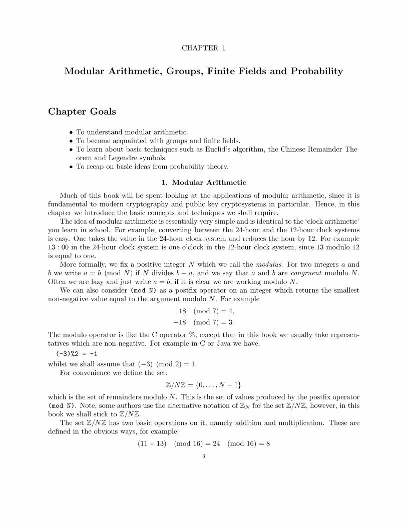
CHAPTER 1
Modular Arithmetic, Groups, Finite Fields and Probability
Chapter Goals
• To understand modular arithmetic.• To become acquainted with groups and finite fields.• To learn about basic techniques such as Euclid’s algorithm, the Chinese Remainder The-
orem and Legendre symbols.• To recap on basic ideas from probability theory.
1. Modular Arithmetic
Much of this book will be spent looking at the applications of modular arithmetic, since it isfundamental to modern cryptography and public key cryptosystems in particular. Hence, in thischapter we introduce the basic concepts and techniques we shall require.
The idea of modular arithmetic is essentially very simple and is identical to the ‘clock arithmetic’you learn in school. For example, converting between the 24-hour and the 12-hour clock systemsis easy. One takes the value in the 24-hour clock system and reduces the hour by 12. For example13 : 00 in the 24-hour clock system is one o’clock in the 12-hour clock system, since 13 modulo 12is equal to one.
More formally, we fix a positive integer N which we call the modulus. For two integers a andb we write a = b (mod N) if N divides b − a, and we say that a and b are congruent modulo N .Often we are lazy and just write a = b, if it is clear we are working modulo N .
We can also consider (mod N) as a postfix operator on an integer which returns the smallestnon-negative value equal to the argument modulo N . For example
18 (mod 7) = 4,
−18 (mod 7) = 3.
The modulo operator is like the C operator %, except that in this book we usually take represen-tatives which are non-negative. For example in C or Java we have,(-3)%2 = -1
whilst we shall assume that (−3) (mod 2) = 1.For convenience we define the set:
Z/NZ = {0, . . . , N − 1}which is the set of remainders modulo N . This is the set of values produced by the postfix operator(mod N). Note, some authors use the alternative notation of ZN for the set Z/NZ, however, in thisbook we shall stick to Z/NZ.
The set Z/NZ has two basic operations on it, namely addition and multiplication. These aredefined in the obvious ways, for example:
(11 + 13) (mod 16) = 24 (mod 16) = 8
3
4 1. MODULAR ARITHMETIC, GROUPS, FINITE FIELDS AND PROBABILITY
since 24 = 1 · 16 + 8 and
(11 · 13) (mod 16) = 143 (mod 16) = 15
since 143 = 8 · 16 + 15.
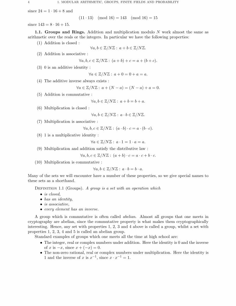
1.1. Groups and Rings. Addition and multiplication modulo N work almost the same asarithmetic over the reals or the integers. In particular we have the following properties:
(1) Addition is closed :∀a, b ∈ Z/NZ : a+ b ∈ Z/NZ.
(2) Addition is associative :
∀a, b, c ∈ Z/NZ : (a+ b) + c = a+ (b+ c).
(3) 0 is an additive identity :
∀a ∈ Z/NZ : a+ 0 = 0 + a = a.
(4) The additive inverse always exists :
∀a ∈ Z/NZ : a+ (N − a) = (N − a) + a = 0.
(5) Addition is commutative :
∀a, b ∈ Z/NZ : a+ b = b+ a.
(6) Multiplication is closed :
∀a, b ∈ Z/NZ : a · b ∈ Z/NZ.
(7) Multiplication is associative :
∀a, b, c ∈ Z/NZ : (a · b) · c = a · (b · c).(8) 1 is a multiplicative identity :
∀a ∈ Z/NZ : a · 1 = 1 · a = a.
(9) Multiplication and addition satisfy the distributive law :
∀a, b, c ∈ Z/NZ : (a+ b) · c = a · c+ b · c.(10) Multiplication is commutative :
∀a, b ∈ Z/NZ : a · b = b · a.Many of the sets we will encounter have a number of these properties, so we give special names tothese sets as a shorthand.
Definition 1.1 (Groups). A group is a set with an operation which• is closed,• has an identity,• is associative,• every element has an inverse.
A group which is commutative is often called abelian. Almost all groups that one meets incryptography are abelian, since the commutative property is what makes them cryptographicallyinteresting. Hence, any set with properties 1, 2, 3 and 4 above is called a group, whilst a set withproperties 1, 2, 3, 4 and 5 is called an abelian group.
Standard examples of groups which one meets all the time at high school are:• The integer, real or complex numbers under addition. Here the identity is 0 and the inverse
of x is −x, since x+ (−x) = 0.• The non-zero rational, real or complex numbers under multiplication. Here the identity is
1 and the inverse of x is x−1, since x · x−1 = 1.
1. MODULAR ARITHMETIC 5
A group is called multiplicative if we tend to write its group operation in the same way as one doesfor multiplication, i.e.
f = g · h and g5 = g · g · g · g · g.We use the notation (G, ·) in this case if there is some ambiguity as to which operation on G weare considering. A group is called additive if we tend to write its group operation in the same wayas one does for addition, i.e.
f = g + h and 5 · g = g + g + g + g + g.
In this case we use the notation (G,+) if there is some ambiguity. An abelian group is called cyclicif there is a special element, called the generator, from which every other element can be obtainedeither by repeated application of the group operation, or by the use of the inverse operation. Forexample, in the integers under addition every positive integer can be obtained by repeated additionof 1 to itself, e.g. 7 can be expressed by
7 = 1 + 1 + 1 + 1 + 1 + 1 + 1.
Every negative integer can be obtained from a positive integer by application of the additive inverseoperator, x→ −x. Hence, we have that 1 is a generator of the integers under addition.
If g is a generator of the cyclic group G we often write G = 〈g〉. If G is multiplicative thenevery element h of G can be written as
h = gx,
whilst if G is additive then every element h of G can be written as
h = x · g,where x in both cases is some integer called the discrete logarithm of h to the base g.
As well as groups we also define the concept of a ring.
Definition 1.2 (Rings). A ring is a set with two operations, usually denoted by + and · foraddition and multiplication, which satisfies properties 1 to 9 above. We can denote a ring and itstwo operations by the triple (R, ·,+).
If it also happens that multiplication is commutative we say that the ring is commutative.
This may seem complicated but it sums up the type of sets one deals with all the time, forexample the infinite commutative rings of integers, real or complex numbers. In fact in cryptographythings are even easier since we only need to consider finite rings, like the commutative ring of integersmodulo N , Z/NZ.
1.2. Euler’s φ Function. In modular arithmetic it will be important to know when, given aand b, the equation
a · x = b (mod N)has a solution. For example there is exactly one solution to the equation
7x = 3 (mod 143),
but there are no solutions to the equation
11x = 3 (mod 143),
however there are 11 solutions to the equation
11x = 22 (mod 143).
Luckily, it is very easy to test when such an equation has one, many or no solutions. We simplycompute the greatest common divisor, or gcd, of a and N , i.e. gcd(a,N).
6 1. MODULAR ARITHMETIC, GROUPS, FINITE FIELDS AND PROBABILITY
• If gcd(a,N) = 1 then there is exactly one solution. We find the value c such that a · c = 1(mod N) and then we compute x = b · c (mod N).
• If g = gcd(a,N) �= 1 and gcd(a,N) divides b then there are g solutions. Here we dividethe whole equation by g to produce the equation
a′ · x′ = b′ (mod N ′),
where a′ = a/g, b′ = b/g and N ′ = N/g. If x′ is a solution to the above equation then
x = x′ + i ·N ′
for 0 ≤ i < g is a solution to the original one.• Otherwise there are no solutions.
The case where gcd(a,N) = 1 is so important we have a special name for it, we say a and N arerelatively prime or coprime.
The number of integers in Z/NZ which are relatively prime to N is given by the Euler φfunction, φ(N). Given the prime factorization of N it is easy to compute the value of φ(N). If Nhas the prime factorization
N =n∏i=1
peii
then
φ(N) =n∏i=1
pei−1i (pi − 1).
Note, the last statement it is very important for cryptography: Given the factorization of N it iseasy to compute the value of φ(N). The most important cases for the value of φ(N) in cryptographyare:
(1) If p is prime thenφ(p) = p− 1.
(2) If p and q are both prime and p �= q then
φ(p · q) = (p− 1)(q − 1).
1.3. Multiplicative Inverse Modulo N . We have just seen that when we wish to solveequations of the form
ax = b (mod N)we reduce to the question of examining when an integer a modulo N has a multiplicative inverse,i.e. whether there is a number c such that
ac = ca = 1 (mod N).
Such a value of c is often written a−1. Clearly a−1 is the solution to the equation
ax = 1 (mod N).
Hence, the inverse of a only exists when a and N are coprime, i.e. gcd(a,N) = 1. Of particularinterest is when N is a prime p, since then for all non-zero values of a ∈ Z/pZ we always obtain aunique solution to
ax = 1 (mod p).Hence, if p is a prime then every non-zero element in Z/pZ has a multiplicative inverse. A ring likeZ/pZ with this property is called a field.
Definition 1.3 (Fields). A field is a set with two operations (G, ·,+) such that• (G,+) is an abelian group with identity denoted by 0,• (G \ {0}, ·) is an abelian group,• (G, ·,+) satisfies the distributive law.
2. FINITE FIELDS 7
Hence, a field is a commutative ring for which every non-zero element has a multiplicativeinverse. You have met fields before, for example consider the infinite fields of rational, real orcomplex numbers.
We define the set of all invertible elements in Z/NZ by
(Z/NZ)∗ = {x ∈ Z/NZ : gcd(x,N) = 1}The ∗ in A∗ for any ring A refers to the largest subset of A which forms a group under multiplication.Hence, the set (Z/NZ)∗ is a group with respect to multiplication and it has size φ(N).
In the special case when N is a prime p we have
(Z/pZ)∗ = {1, . . . , p− 1}since every non-zero element of Z/pZ is coprime to p. For an arbitrary field F the set F ∗ is equalto the set F \ {0}. To ease notation, for this very important case, define
Fp = Z/pZ = {0, . . . , p− 1}and
F∗p = (Z/pZ)∗ = {1, . . . , p− 1}.
The set Fp is a finite field of characteristic p. In the next section we shall discuss a more generaltype of finite field, but for now recall the important point that the integers modulo N are only afield when N is a prime.
We end this section with the most important theorem in elementary group theory.
Theorem 1.4 (Lagrange’s Theorem). If (G, ·) is a group of order (size) n = #G then for alla ∈ G we have an = 1.
So if x ∈ (Z/NZ)∗ thenxφ(N) = 1 (mod N)
since #(Z/NZ)∗ = φ(N). This leads us to Fermat’s Little Theorem, not to be confused withFermat’s Last Theorem which is something entirely different.
Theorem 1.5 (Fermat’s Little Theorem). Suppose p is a prime and a ∈ Z then
ap = a (mod p).
Fermat’s Little Theorem is a special case of Lagrange’s Theorem and will form the basis of oneof the primality tests considered in a later chapter.
2. Finite Fields
The integers modulo a prime p are not the only types of finite field. In this section we shallintroduce another type of finite field which is particularly important. At first reading you may wishto skip this section. We shall only be using these general forms of finite fields when discussing theRijndael block cipher, stream ciphers based on linear feedback shift registers and when we look atelliptic curve based systems.
For this section we let p denote a prime number. Consider the set of polynomials in X whosecoefficients are reduced modulo p. We denote this set Fp[X], which forms a ring with the naturaldefinition of addition and multiplication.
Of particular interest is the case when p = 2, from which we draw all our examples in thissection. For example, in F2[X] we have
(1 +X +X2) + (X +X3) = 1 +X2 +X3,
(1 +X +X2) · (X +X3) = X +X2 +X4 +X5.
8 1. MODULAR ARITHMETIC, GROUPS, FINITE FIELDS AND PROBABILITY
Just as with the integers modulo a number N , where the integers modulo N formed a ring, we cantake a polynomial f(X) and then the polynomials modulo f(X) also form a ring. We denote thisring by
Fp[X]/f(X)Fp[X]
or more simplyFp[X]/(f(X)).
But to ease notation we will often write Fp[X]/f(X) for this latter ring. When f(X) = X4 +1 andp = 2 we have, for example,
(1 +X +X2) · (X +X3) (mod X4 + 1) = 1 +X2
sinceX +X2 +X4 +X5 = (X + 1) · (X4 + 1) + (1 +X2).
When checking the above equation you should remember we are working modulo two.
Recall, when we looked at the integers modulo N we looked at the equation
ax = b (mod N).
We can consider a similar question for polynomials. Given a, b and f , all of which are polynomialsin Fp[X], does there exist a solution α to the equation
aα = b (mod f)?
With integers the answer depended on the greatest common divisor of a and f , and we countedthree possible cases. A similar three cases can occur for polynomials, with the most important onebeing when a and f are coprime and so have greatest common divisor equal to one.
A polynomial is called irreducible if it has no proper factors other than itself and the constantpolynomials. Hence, irreducibility of polynomials is the same as primality of numbers. Just as withthe integers modulo N , when N was prime we obtained a finite field, so when f(X) is irreduciblethe ring Fp[X]/f(X) also forms a finite field.
Consider the case p = 2 and the two different irreducible polynomials
f1 = X7 +X + 1
andf2 = X7 +X3 + 1.
Now, consider the two finite fields
F1 = F2[X]/f1(X) and F2 = F2[X]/f2(X).
These both consist of the 27 binary polynomials of degree less than seven. Addition in these twofields is identical in that one just adds the coefficients of the polynomials modulo two. The onlydifference is in how multiplication is performed
(X3 + 1) · (X4 + 1) (mod f1(X)) = X4 +X3 +X,
(X3 + 1) · (X4 + 1) (mod f2(X)) = X4.
A natural question arises as to whether these fields are ‘really’ different, or whether they just “look”different. In mathematical terms the question is whether the two fields are isomorphic. It turnsout that they are isomorphic if there is a map
φ : F1 −→ F2,
2. FINITE FIELDS 9
called a field isomorphism, which satisfies
φ(α+ β) = φ(α) + φ(β),
φ(α · β) = φ(α) · φ(β).
Such an isomorphism exists for every two finite fields of the same order, although we will not showit here. To describe the map above you only need to show how to express a root of f2(X) in termsof a polynomial in the root of f1(X).
The above construction is in fact the only way of producing finite fields, hence all finite fieldsare essentially equal to polynomials modulo a prime and modulo an irreducible polynomial (forthat prime). Hence, we have the following basic theorem
Theorem 1.6. There is (up to isomorphism) just one finite field of each prime power order.
The notation we use for these fields is either Fq or GF (q), with q = pd where d is the degree ofthe irreducible polynomial used to construct the finite field. We of course have Fp = Fp[X]/X. Thenotation GF (q) means the Galois field of q elements. Finite fields are sometimes named after the19th century French mathematician Galois. Galois had an interesting life, he accomplished mostof his scientific work at an early age before dying in a duel.
There are a number of technical definitions associated with finite fields which we need to cover.Each finite field K contains a copy of the integers modulo p for some prime p, we call this primethe characteristic of the field, and often write this as char K. The subfield of integers modulo p ofa finite field is called the prime subfield.
There is a map Φ called the p-th power Frobenius map defined for any finite field by
Φ :{
Fq −→ Fq
α −→ αp
where p is the characteristic of Fq. The Frobenius map is an isomorphism of Fq with itself, such anisomorphism is called an automorphism. An interesting property is that the set of elements fixedby the Frobenius map is the prime field, i.e.
{α ∈ Fq : αp = α} = Fp.
Notice that this is a kind of generalization of Fermat’s Little Theorem to finite fields. For anyautomorphism χ of a finite field the set of elements fixed by χ is a field, called the fixed field of χ.Hence the previous statement says that the fixed field of the Frobenius map is the prime field Fp.
Not only does Fq contain a copy of Fp but Fpd contains a copy of Fpe for every value of e dividingd. In addition Fpe is the fixed field of the automorphism Φe, i.e.
{α ∈ Fpd : αpe
= α} = Fpe .
Another interesting property is that if p is the characteristic of Fq then if we take any elementα ∈ Fq and add it to itself p times we obtain zero, e.g. in F49 we have
X +X +X +X +X +X +X = 7X = 0 (mod 7).
The non-zero elements of a finite field, usually denoted F∗q, form a cyclic finite abelian group. We
call a generator of F∗q a primitive element in the finite field. Such primitive elements always exist
and so the multiplicative group is always cyclic. In other words there always exists an elementg ∈ Fq such that every non-zero element α can be written as
α = gx
for some integer value of x.As an example consider the field of eight elements defined by
F23 = F2[X]/(X3 +X + 1).
10 1. MODULAR ARITHMETIC, GROUPS, FINITE FIELDS AND PROBABILITY
In this field there are seven non-zero elements namely
1, α, α + 1, α2, α2 + 1, α2 + α,α2 + α+ 1
where α is a root of X3 +X + 1. We see that α is a primitive element in F23 since
α1 = α,
α2 = α2,
α3 = α+ 1,
α4 = α2 + α,
α5 = α2 + α+ 1,
α6 = α2 + 1,
α7 = 1.
Notice that for a prime p this means that the integers modulo a prime also have a primitive element,since Z/pZ = Fp is a finite field.
3. Basic Algorithms
There are several basic numerical algorithms or techniques which everyone should know sincethey occur in many places in this book. The ones we shall concentrate on here are
• Euclid’s gcd algorithm,• the Chinese Remainder Theorem,• computing Jacobi and Legendre symbols.
3.1. Greatest Common Divisors. In the previous sections we said that when trying to solve
a · x = b (mod N)
in integers, oraα = b (mod f)
for polynomials modulo a prime, we needed to compute the greatest common divisor. This wasparticularly important in determining whether a ∈ Z/NZ or a ∈ Fp[X]/f had a multiplicativeinverse or not, i.e. gcd(a,N) = 1 or gcd(a, f) = 1. We did not explain how this greatest commondivisor is computed, neither did we explain how the inverse is to be computed when we know itexists. We shall now address this omission by explaining one of the oldest algorithms known toman, namely the Euclidean algorithm.
If we were able to factor a and N into primes, or a and f into irreducible polynomials, thencomputing the greatest common divisor would be particularly easy. For example if
a = 230 895 588 646 864 = 24 · 157 · 45133,
b = 33107 658 350 407 876 = 22 · 157 · 22693 · 4513,then it is easy, from the factorization, to compute the gcd as
gcd(a, b) = 22 · 157 · 4513 = 2834 164.
However, factoring is an expensive operation for integers, but computing greatest common divisorsis easy as we shall show. Although factoring for polynomials modulo a prime is very easy, it turnsout that almost all algorithms to factor polynomials require access to an algorithm to computegreatest common divisors. Hence, in both situations we need to be able to compute greatestcommon divisors without recourse to factoring.
3. BASIC ALGORITHMS 11
3.1.1. Euclidean Algorithm: In the following we will consider the case of integers only, thegeneralization to polynomials is easy since both integers and polynomials allow Euclidean division.For integers Euclidean division is the operation of, given a and b, finding q and r with 0 ≤ r < |b|such that
a = q · b+ r.
For polynomials Euclidean division is given polynomials f, g finding polynomials q, r with 0 ≤deg r < deg g such that
f = q · g + r.
To compute the gcd of r0 = a and r1 = b we compute r2, r3, r4, . . . as follows;
r2 = q1r1 − r0
r3 = q2r2 − r1
......
rm = qm−1rm−1 − rm−2
rm+1 = qmrm.
If d divides a and b then d divides r2, r3, r4 and so on. Hence
gcd(a, b) = gcd(r0, r1) = gcd(r1, r2) = · · · = gcd(rm−1, rm) = rm.
As an example of this algorithm we want to show that
3 = gcd(21, 12).
Using the Euclidean algorithm we compute gcd(21, 12) in the steps
gcd(21, 12) = gcd(21 (mod 12), 12)
= gcd(9, 12)
= gcd(12 (mod 9), 9)
= gcd(3, 9)
= gcd(9 (mod 3), 3)
= gcd(0, 3) = 3.
Or, as an example with larger numbers,
gcd(1 426 668 559 730, 810 653 094 756) = gcd(810 653 094 756, 616 015 464 974),
= gcd(616 015 464 974, 194 637 629 782),
= gcd(194 637 629 782, 32 102 575 628),
= gcd(32 102 575 628, 2 022 176 014),
= gcd(2 022 176 014, 1 769 935 418),
= gcd(1 769 935 418, 252 240 596),
= gcd(252 240 596, 4 251 246),
= gcd(4 251 246, 1 417 082),
= gcd(1 417 082, 0),= 1417 082.
The Euclidean algorithm essentially works because the map
(a, b) −→ (a (mod b), b),
for a ≥ b is a gcd preserving mapping. The trouble is that computers find it much easier to addand multiply numbers than to take remainders or quotients. Hence, implementing a gcd algorithm
12 1. MODULAR ARITHMETIC, GROUPS, FINITE FIELDS AND PROBABILITY
with the above gcd preserving mapping will usually be very inefficient. Fortunately, there are anumber of other gcd preserving mappings, for example
(a, b) −→
⎧⎪⎨⎪⎩
((a− b)/2, b) If a and b are odd.(a/2, b) If a is even and b is odd.(a, b/2) If a is odd and b is even.
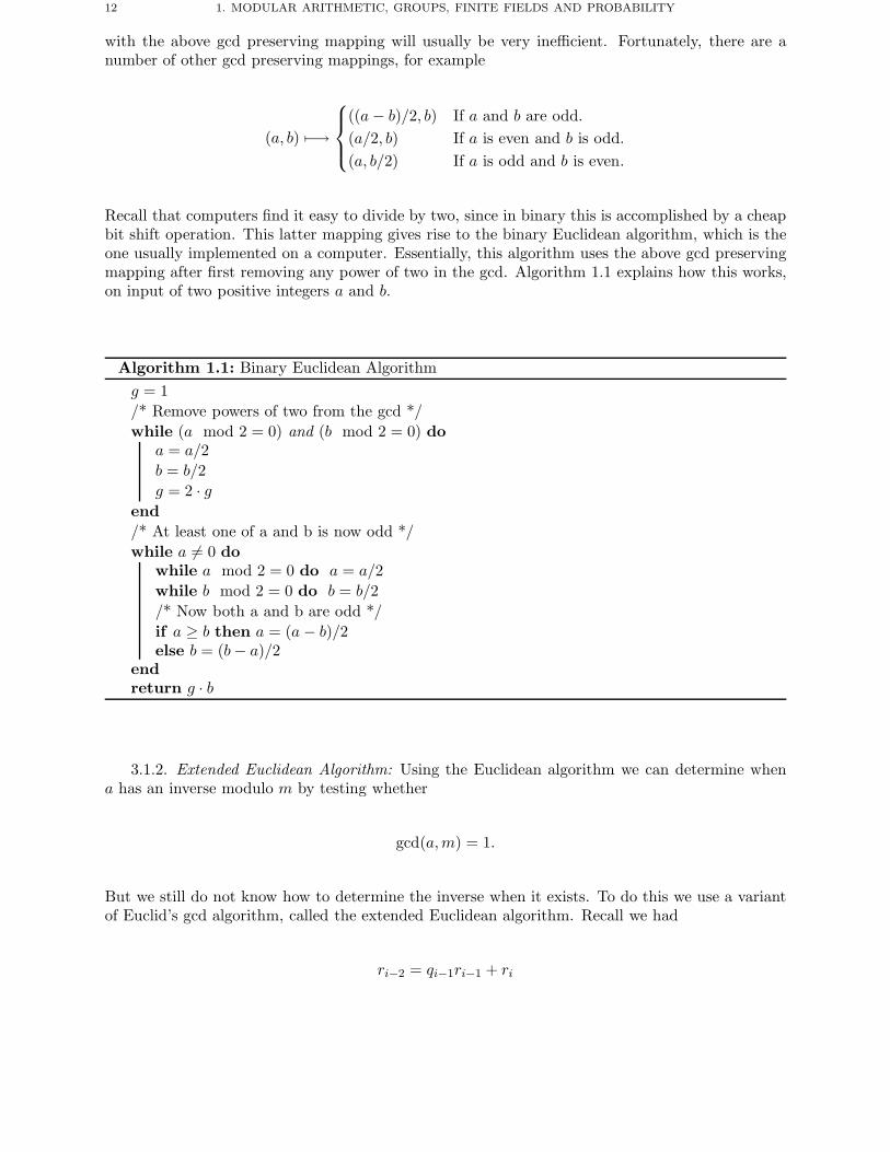
Recall that computers find it easy to divide by two, since in binary this is accomplished by a cheapbit shift operation. This latter mapping gives rise to the binary Euclidean algorithm, which is theone usually implemented on a computer. Essentially, this algorithm uses the above gcd preservingmapping after first removing any power of two in the gcd. Algorithm 1.1 explains how this works,on input of two positive integers a and b.
Algorithm 1.1: Binary Euclidean Algorithmg = 1/* Remove powers of two from the gcd */while (a mod 2 = 0) and (b mod 2 = 0) do
a = a/2b = b/2g = 2 · g
end/* At least one of a and b is now odd */while a �= 0 do
while a mod 2 = 0 do a = a/2while b mod 2 = 0 do b = b/2/* Now both a and b are odd */if a ≥ b then a = (a− b)/2else b = (b− a)/2
endreturn g · b
3.1.2. Extended Euclidean Algorithm: Using the Euclidean algorithm we can determine whena has an inverse modulo m by testing whether
gcd(a,m) = 1.
But we still do not know how to determine the inverse when it exists. To do this we use a variantof Euclid’s gcd algorithm, called the extended Euclidean algorithm. Recall we had
ri−2 = qi−1ri−1 + ri
3. BASIC ALGORITHMS 13
with rm = gcd(r0, r1). Now we unwind the above and write each ri, for i ≥ 2, in terms of a and b.For example
r2 = r0 − q1r1 = a− q1b
r3 = r1 − q2r2 = b− q2(a− q1b) = −q2a+ (1 + q1q2)b...
...ri−2 = si−2a+ ti−2b
ri−1 = si−1a+ ti−1b
ri = ri−2 − qi−1ri−1
= a(si−2 − qi−1si−1) + b(ti−2 − qi−1ti−1)...
...rm = sma+ tmb.
The extended Euclidean algorithm takes as input a and b and outputs rm, sm and tm such that
rm = gcd(a, b) = sma+ tmb.
Hence, we can now solve our original problem of determining the inverse of a modulo N , when suchan inverse exists. We first apply the extended Euclidean algorithm to a and N so as to computed, x, y such that
d = gcd(a,N) = xa+ yN.
We can solve the equation ax = 1 (mod N), since we have d = xa + yN = xa (mod N). Hence,we have a solution x = a−1, precisely when d = 1.
As an example suppose we wish to compute the inverse of 7 modulo 19. We first set r0 = 7 andr1 = 19 and then we compute
r2 = 5 = 19 − 2 · 7r3 = 2 = 7 − 5 = 7 − (19 − 2 · 7) = −19 + 3 · 7r4 = 1 = 5 − 2 · 2 = (19 − 2 · 7) − 2 · (−19 + 3 · 7) = 3 · 19 − 8 · 7.
Hence,1 = −8 · 7 (mod 19)
and so7−1 = −8 = 11 (mod 19).
3.2. Chinese Remainder Theorem (CRT). The Chinese Remainder Theorem, or CRT, isalso a very old piece of mathematics, which dates back at least 2000 years. We shall use the CRTin a few places, for example to improve the performance of the decryption operation of RSA andin a number of other protocols. In a nutshell the CRT states that if we have the two equations
x = a (mod N) and x = b (mod M)
then there is a unique solution modulo M ·N if and only if gcd(N,M) = 1. In addition it gives amethod to easily find the solution. For example if the two equations are given by
x = 4 (mod 7),
x = 3 (mod 5),
then we havex = 18 (mod 35).
It is easy to check that this is a solution, since 18 (mod 7) = 4 and 18 (mod 5) = 3. But how didwe produce this solution?
14 1. MODULAR ARITHMETIC, GROUPS, FINITE FIELDS AND PROBABILITY
We shall first show how this can be done naively from first principles and then we shall givethe general method. We have the equations
x = 4 (mod 7) and x = 3 (mod 5).
Hence for some u we havex = 4 + 7u and x = 3 (mod 5).
Putting these latter two equations into one gives,
4 + 7u = 3 (mod 5).
We then rearrange the equation to find
2u = 7u = 3 − 4 = 4 (mod 5).
Now since gcd(2, 5) = gcd(7, 5) = 1 we can solve the above equation for u. First we compute 2−1
(mod 5) = 3, since 2 · 3 = 6 = 1 (mod 5). Then we compute the value of u = 3 · 4 (mod 5). Thensubstituting this value of u back into our equation for x gives the solution
x = 4 + 7u = 4 + 7 · 2 = 18.
The case of two equations is so important we now give a general formula. We assume thatgcd(N,M) = 1, and that we are given the equations
x = a (mod M) and x = b (mod N).
We first computeT = M−1 (mod N)
which is possible since we have assumed gcd(N,M) = 1. We then compute
u = (b− a)T (mod N).
The solution modulo M ·N is then given by
x = a+ uM.
To see this always works we compute
x (mod M) = a+ uM (mod M)= a,
x (mod N) = a+ uM (mod N)
= a+ (b− a)TM (mod N)
= a+ (b− a)M−1M (mod N)
= a+ (b− a) (mod N)= b.
Now we turn to the general case of the CRT where we consider more than two equations atonce. Let m1, . . . ,mr be pairwise relatively prime and let a1, . . . , ar be given. We want to find xmodulo M = m1m2 · · ·mr such that
x = ai (mod mi) for all i.
The Chinese Remainder Theorem guarantees a unique solution given by
x =r∑i=1
aiMiyi (mod M)
3. BASIC ALGORITHMS 15
where
Mi = M/mi,
yi = M−1i (mod mi).
As an example suppose we wish to find the unique x modulo
M = 1001 = 7 · 11 · 13such that
x = 5 (mod 7),
x = 3 (mod 11),
x = 10 (mod 13).
We computeM1 = 143, y1 = 5,M2 = 91, y2 = 4,M3 = 77, y3 = 12.
Then, the solution is given by
x =r∑i=1
aiMiyi (mod M)
= 715 · 5 + 364 · 3 + 924 · 10 (mod 1001)= 894.
3.3. Legendre and Jacobi Symbols. Let p denote a prime, greater than two. Consider themapping
Fp −→ Fp
α −→ α2.
This mapping is exactly two-to-one on the non-zero elements of Fp. So if an element x in Fp has asquare root, then it has exactly two square roots (unless x = 0) and exactly half of the elements ofF∗p are squares. The set of squares in F∗
p are called the quadratic residues and they form a subgroup,of order (p − 1)/2 of the multiplicative group F∗
p. The elements of F∗p which are not squares are
called the quadratic non-residues.To make it easy to detect squares modulo p we define the Legendre symbol(
a
p
).
This is defined to be equal to 0 if p divides a, it is equal to +1 if a is a quadratic residue and it isequal to −1 if a is a quadratic non-residue.
It is easy to compute the Legendre symbol, for example via(a
p
)= a(p−1)/2 (mod p).
However, using the above formula turns out to be very inefficient. In practice one uses the law ofquadratic reciprocity
(1)(q
p
)=(p
q
)(−1)(p−1)(q−1)/4 .
16 1. MODULAR ARITHMETIC, GROUPS, FINITE FIELDS AND PROBABILITY
In other words we have
(q
p
)=
⎧⎪⎪⎨⎪⎪⎩−(p
q
)If p = q = 3 (mod 4),(
p
q
)Otherwise
Using this law with the following additional formulae gives rise to a recursive algorithm(q
p
)=(q (mod p)
p
),(2) (
q · rp
)=(q
p
)·(r
p
),(3) (
2p
)= (−1)(p
2−1)/8.(4)
Assuming we can factor, we can now compute the Legendre symbol(1517
)=(
317
)·(
517
)by Equation (3)
=(
173
)·(
175
)by Equation (1)
=(
23
)·(
25
)by Equation (2)
= (−1) · (−1)3 by Equation (4)= 1.
In a moment we shall see a more efficient algorithm which does not require us to factor integers.
Computing square roots of elements in F∗p, when the square root exists turns out to be an easy
task. Algorithm 1.2 gives one method, called Shanks’ Algorithm, of computing the square root ofa modulo p, when such a square root exists.
When p = 3 (mod 4), instead of the above algorithm, we can use the following formulae
x = a(p+1)/4 (mod p),
which has the advantage of being deterministic and more efficient than the general method ofShanks. That this formula works is because
x2 = a(p+1)/2 = a(p−1)/2 · a =(a
p
)· a = a
where the last equality holds since we have assumed that a is a quadratic residue modulo p and soit has Legendre symbol equal to one.
The Legendre symbol above is only defined when its denominator is a prime, but there is ageneralization to composite denominators called the Jacobi symbol. Suppose n ≥ 3 is odd and
n = pe11 pe22 · · · pekk
then the Jacobi symbol (an
)is defined in terms of the Legendre symbol by(a
n
)=(a
p1
)e1 ( ap2
)e2· · ·(a
pk
)ek.
3. BASIC ALGORITHMS 17
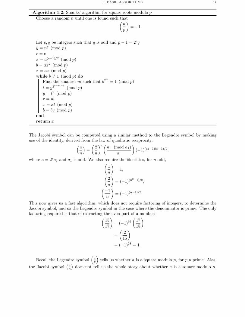
Algorithm 1.2: Shanks’ algorithm for square roots modulo pChoose a random n until one is found such that(
n
p
)= −1
Let e, q be integers such that q is odd and p− 1 = 2eqy = nq (mod p)r = e
x = a(q−1)/2 (mod p)b = ax2 (mod p)x = ax (mod p)while b �= 1 (mod p) do
Find the smallest m such that b2m
= 1 (mod p)t = y2r−m−1
(mod p)y = t2 (mod p)r = m
x = xt (mod p)b = by (mod p)
endreturn x
The Jacobi symbol can be computed using a similar method to the Legendre symbol by makinguse of the identity, derived from the law of quadratic reciprocity,(a
n
)=(
2n
)e(n (mod a1)a1
)(−1)(a1−1)(n−1)/4.
where a = 2ea1 and a1 is odd. We also require the identities, for n odd,(1n
)= 1,(
2n
)= (−1)(n
2−1)/8,(−1n
)= (−1)(n−1)/2.
This now gives us a fast algorithm, which does not require factoring of integers, to determine theJacobi symbol, and so the Legendre symbol in the case where the denominator is prime. The onlyfactoring required is that of extracting the even part of a number:(
1517
)= (−1)56
(1715
)
=(
215
)= (−1)28 = 1.
Recall the Legendre symbol(ap
)tells us whether a is a square modulo p, for p a prime. Alas,
the Jacobi symbol(an
)does not tell us the whole story about whether a is a square modulo n,
18 1. MODULAR ARITHMETIC, GROUPS, FINITE FIELDS AND PROBABILITY
when n is a composite. If a is a square modulo n then the Jacobi symbol will be equal to plus one,however if the Jacobi symbol is equal to plus one then it is not always true that a is a square.
Let n ≥ 3 be odd and let the set of squares in (Z/nZ)∗ be denoted
Qn = {x2 (mod n) : x ∈ (Z/nZ)∗}.Now let Jn denote the set of elements with Jacobi symbol equal to plus one, i.e.
Jn ={x ∈ (Z/nZ)∗ :
(an
)= 1}.
The set of pseudo-squares is the difference Jn \Qn.There are two important cases for cryptography, either n is prime or n is the product of two
primes:• n is a prime p.
• Qn = Jn.• #Qn = (n− 1)/2.
• n is the product of two primes, n = p · q.• Qn ⊂ Jn.• #Qn = #(Jn \Qn) = (p− 1)(q − 1)/4.
The sets Qn and Jn will be seen to be important in a number of algorithms and protocols, especiallyin the case where n is a product of two primes.
Finally, we look at how to compute a square root modulo a composite number n = p·q. Supposewe wish to compute the square root of a modulo n. We assume we know p and q, and that a reallyis a square modulo n, which can be checked by demonstrating that(
a
p
)=(a
q
)= 1.
We first compute the square root of a modulo p, call this sp. Then we compute the square rootof a modulo q, call this sq. Finally to deduce the square root modulo n, we apply the ChineseRemainder Theorem to the equations
x = sp (mod p) and x = sq (mod q).
As an example suppose we wish to compute the square root of a = 217 modulo n = 221 = 13 · 17.Now the square root of a modulo 13 and 17 is given by
s13 = 3 and s17 = 8.
Applying the Chinese Remainder Theorem we find
s = 42
and we can check that s really is a square root by computing
s2 = 422 = 217 (mod n).
There are three other square roots, since n has two prime factors. These other square roots areobtained by applying the Chinese Remainder Theorem to the three other equations
s13 = 10, s17 = 8,s13 = 3, s17 = 9,s13 = 10, s17 = 9,
Hence, all four square roots of 217 modulo 221 are given by
42, 94, 127 and 179.
4. PROBABILITY 19
4. Probability
At some points we will need a basic understanding of elementary probability theory. In thissection we summarize the theory we require and give a few examples. Most readers should find thisa revision of the type of probability encountered in high school.
A random variable is a variable X which takes certain values with given probabilities. If Xtakes on the value s with probability 0.01 we write this as
p(X = s) = 0.01.
As an example, let T be the random variable representing tosses of a fair coin, we then have theprobabilities
p(T = Heads) =12,
p(T = Tails) =12.
As another example let E be the random variable representing letters in English text. An analysisof a large amount of English text allows us to approximate the relevant probabilities by
p(E = a) = 0.082,...
p(E = e) = 0.127,...
p(E = z) = 0.001.
Basically if X is a discrete random variable and p(X = x) is the probability distribution then wehave the two following properties:
p(X = x) ≥ 0,∑x
p(X = x) = 1.
It is common to illustrate examples from probability theory using a standard deck of cards. Weshall do likewise and let V denote the random variable that a card is a particular value, let S denotethe random variable that a card is a particular suit and let C denote the random variable of thecolour of a card. So for example
p(C = Red) =12,
p(V = Ace of Clubs) =152,
p(S = Clubs) =14.
Let X and Y be two random variables, where p(X = x) is the probability that X takes the valuex and p(Y = y) is the probability that Y takes the value y. The joint probability p(X = x, Y = y)is defined as the probability that X takes the value x and Y takes the value y. So if we let X = C
20 1. MODULAR ARITHMETIC, GROUPS, FINITE FIELDS AND PROBABILITY
and Y = S then we have
p(C = Red, S = Club) = 0, p(C = Red, S = Diamonds) =14,
p(C = Red, S = Hearts) =14, p(C = Red, S = Spades) = 0,
p(C = Black, S = Club) =14, p(C = Black, S = Diamonds) = 0,
p(C = Black, S = Hearts) = 0, p(C = Black, S = Spades) =14.
Two random variables X and Y are said to be independent if, for all values of x and y,
p(X = x, Y = y) = p(X = x) · p(Y = y).
Hence, the random variables C and S are not independent. As an example of independent randomvariables consider the two random variables, T1 the value of the first toss of an unbiased coin andT2 the value of a second toss of the coin. Since, assuming standard physical laws, the toss of thefirst coin does not affect the outcome of the toss of the second coin, we say that T1 and T2 areindependent. This is confirmed by the joint probability distribution
p(T1 = H,T2 = H) =14, p(T1 = H,T2 = T ) =
14,
p(T1 = T, T2 = H) =14, p(T1 = T, T2 = T ) =
14.
4.1. Bayes’ Theorem. The conditional probability p(X = x|Y = y) of two random variablesX and Y is defined as the probability that X takes the value x given that Y takes the value y.
Returning to our random variables based on a pack of cards we have
p(S = Spades|C = Red) = 0
and
p(V = Ace of Spades|C = Black) =126.
The first follows since if we know a card is red, then the probability that it is a spade is zero, sincea red card cannot be a spade. The second follows since if we know a card is black then we haverestricted the set of cards in half, one of which is the ace of spades.
The following is one of the most crucial statements in probability theory
Theorem 1.7 (Bayes’ Theorem). If p(Y = y) > 0 then
p(X = x|Y = y) =p(X = x) · p(Y = y|X = x)
p(Y = y)
=p(X = x, Y = y)
p(Y = y).
We can apply Bayes’ Theorem to our examples above as follows
p(S = Spades|C = Red) =p(S = Spades, C = Red)
p(C = Red)
= 0 ·(
14
)−1
= 0.
Chapter Summary 21
p(V = Ace of Spades|C = Black) =p(V = Ace of Spades, C = Black)
p(C = Black)
=152
·(
12
)−1
=252
=126.
If X and Y are independent then we have
p(X = x|Y = y) = p(X = x),
i.e. the value which X takes does not depend on the value that Y takes.
4.2. Birthday Paradox. Another useful result from elementary probability theory that werequire is the birthday paradox. Suppose a bag has m balls in it, all of different colours. We drawone ball at a time from the bag and write down its colour, we then replace the ball in the bag anddraw again.
If we definem(n) = m · (m− 1) · (m− 2) · · · (m− n+ 1)
then the probability, after n balls have been taken out of the bag, that we have obtained at leastone matching colour (or coincidence) is
1 − m(n)
mn.
As m becomes larger the expected number of balls we have to draw before we obtain the firstcoincidence is √
πm
2.
To see why this is called the birthday paradox consider the probability of two people in a roomsharing the same birthday. Most people initially think that this probability should be quite low,since they are thinking of the probability that someone in the room shares the same birthday asthem. One can now easily compute that the probability of at least two people in a room of 23people having the same birthday is
1 − 365(23)
36523≈ 0.507.
In fact this probability increases quite quickly since in a room of 30 people we obtain a probabilityof approximately 0.706, and in a room of 100 people we obtain a probability of over 0.999 999 6.
Chapter Summary
• A group is a set with an operation which has an identity, is associative and every elementhas an inverse. Modular arithmetic, both addition and multiplication, provides examplesof groups. However, for multiplication we need to be careful which set of numbers we takewhen defining a group with respect to modular multiplication.
• A ring is a set with two operations which behaves like the set of integers under additionand multiplication. Modular arithmetic is an example of a ring.
• A field is a ring in which all non-zero elements have a multiplicative inverse. Integersmodulo a prime are examples of fields.
22 1. MODULAR ARITHMETIC, GROUPS, FINITE FIELDS AND PROBABILITY
• Multiplicative inverses for modular arithmetic can be found using the extended Euclideanalgorithm.
• Sets of simultaneous linear modular equations can be solved using the Chinese RemainderTheorem.
• Square elements modulo a prime can be detected using the Legendre symbol, square rootscan be efficiently computed using Shanks’ Algorithm.
• Square elements and square roots modulo a composite can be determined efficiently aslong as one knows the factorization of the modulus.
• Bayes’ theorem allows us to compute conditional probabilities.• The birthday paradox allows us to estimate how quickly collisions occur when one repeat-
edly samples from a finite space.
Further Reading
Bach and Shallit is the best introductory book I know which deals with Euclid’s algorithmand finite fields. It contains a lot of historical information, plus excellent pointers to the relevantresearch literature. Whilst aimed in some respects at Computer Scientists, Bach and Shallit’s bookmay be a little too mathematical for some. For a more traditional introduction to the basic discretemathematics we shall need, at the level of a first year course in Computer Science, see the booksby Biggs or Rosen.
E. Bach and J. Shallit. Algorithmic Number Theory. Volume 1: Efficient Algorithms. MIT Press,1996.
N.L. Biggs. Discrete Mathematics. Oxford University Press, 1989.
K.H. Rosen. Discrete Mathematics and its Applications. McGraw-Hill, 1999.
CHAPTER 2
Elliptic Curves
Chapter Goals
• To describe what an elliptic curve is.• To explain the basic mathematics behind elliptic curve cryptography.• To show how projective coordinates can be used to improve computational efficiency.• To show how point compression can be used to improve communications efficiency.
1. Introduction
This chapter is devoted to introducing elliptic curves. Some of the more modern public keysystems make use of elliptic curves since they can offer improved efficiency and bandwidth. Sincemuch of this book can be read by understanding that an elliptic curve provides another finiteabelian group in which one can pose a discrete logarithm problem, you may decide to skip thischapter on an initial reading.
Let K be any field. The projective plane P2(K) over K is defined as the set of triples
(X,Y,Z)
where X,Y,Z ∈ K are not all simultaneously zero. On these triples is defined an equivalencerelation
(X,Y,Z) ≡ (X ′, Y ′, Z ′)if there exists a λ ∈ K such that
X = λX ′, Y = λY ′ and Z = λZ ′.
So, for example, if K = F7, the finite field of seven elements, then the two points
(4, 1, 1) and (5, 3, 3)
are equivalent. Such a triple is called a projective point.An elliptic curve over K will be defined as the set of solutions in the projective plane P2(K) of
a homogeneous Weierstrass equation of the form
E : Y 2Z + a1XY Z + a3Y Z2 = X3 + a2X
2Z + a4XZ2 + a6Z
3,
with a1, a2, a3, a4, a6 ∈ K. This equation is also referred to as the long Weierstrass form. Such acurve should be non-singular in the sense that, if the equation is written in the form F (X,Y,Z) = 0,then the partial derivatives of the curve equation
∂F/∂X, ∂F/∂Y and ∂F/∂Z
should not vanish simultaneously at any point on the curve.The set of K-rational points on E, i.e. the solutions in P2(K) to the above equation, is denoted
by E(K). Notice, that the curve has exactly one rational point with coordinate Z equal to zero,namely (0, 1, 0). This is the point at infinity, which will be denoted by O.
23
24 2. ELLIPTIC CURVES
For convenience, we will most often use the affine version of the Weierstrass equation, given by
(5) E : Y 2 + a1XY + a3Y = X3 + a2X2 + a4X + a6,
where ai ∈ K.The K-rational points in the affine case are the solutions to E in K2, plus the point at infinity
O. Although most protocols for elliptic curve based cryptography make use of the affine form of acurve, it is often computationally important to be able to switch to projective coordinates. Luckilythis switch is easy:
• The point at infinity always maps to the point at infinity in either direction.• To map a projective point (X,Y,Z) which is not at infinity, so Z �= 0, to an affine point
we simply compute (X/Z, Y/Z).• To map an affine point (X,Y ), which is not at infinity, to a projective point we take a
random non-zero Z ∈ K and compute (X · Z, Y · Z,Z).As we shall see later it is often more convenient to use a slightly modified form of projective pointwhere the projective point (X,Y,Z) represents the affine point (X/Z2, Y/Z3).
Given an elliptic curve defined by Equation (5), it is useful to define the following constants foruse in later formulae:
b2 = a21 + 4a2,
b4 = a1a3 + 2a4,
b6 = a23 + 4a6,
b8 = a21a6 + 4a2a6 − a1a3a4 + a2a
23 − a2
4,
c4 = b22 − 24b4,
c6 = −b32 + 36b2b4 − 216b6.
The discriminant of the curve is defined as
Δ = −b22b8 − 8b34 − 27b26 + 9b2b4b6.
When char K �= 2, 3 the discriminant can also be expressed as
Δ = (c34 − c26)/1728.
Notice that 1728 = 2633 so, if the characteristic is not equal to 2 or 3, dividing by this latterquantity makes sense. A curve is then non-singular if and only if Δ �= 0; from now on we shallassume that Δ �= 0 in all our discussions.
When Δ �= 0, the j-invariant of the curve is defined as
j(E) = c34/Δ.
As an example, which we shall use throughout this chapter, we consider the elliptic curve
E : Y 2 = X3 +X + 3
defined over the field F7. Computing the various quantities above we find that we have
Δ = 3 and j(E) = 5.
The j-invariant is closely related to the notion of elliptic curve isomorphism. Two elliptic curvesdefined by Weierstrass equations E (with variables X,Y ) and E′ (with variables X ′, Y ′) are iso-morphic over K if and only if there exist constants r, s, t ∈ K and u ∈ K∗, such that the change ofvariables
X = u2X ′ + r , Y = u3Y ′ + su2X ′ + t
2. THE GROUP LAW 25
transforms E into E′. Such an isomorphism defines a bijection between the set of rational pointsin E and the set of rational points in E′. Notice that isomorphism is defined relative to the fieldK.
As an example consider again the elliptic curve
E : Y 2 = X3 +X + 3
over the field F7. Now make the change of variables defined by [u, r, s, t] = [2, 3, 4, 5], i.e.
X = 4X ′ + 3 and Y = Y ′ + 2X ′ + 5.
We then obtain the isomorphic curve
E′ : Y ′2 + 4X ′Y ′ + 3Y ′ = X ′3 +X ′ + 1,
and we havej(E) = j(E′) = 5.
Curve isomorphism is an equivalence relation. The following lemma establishes the fact that,over the algebraic closure K, the j-invariant characterizes the equivalence classes in this relation.
Lemma 2.1. Two elliptic curves that are isomorphic over K have the same j-invariant. Con-versely, two curves with the same j-invariant are isomorphic over K.
But curves with the same j-invariant may not necessarily be isomorphic over the ground field.For example, consider the elliptic curve, also over F7,
E′′ : Y ′′2 = X ′′3 + 4X ′′ + 4.
This has j-invariant equal to 5 so it is isomorphic to E, but it is not isomorphic over F7 since thechange of variable required is given by
X = 3X ′′ and Y =√
6Y ′′.
However,√
6 �∈ F7. Hence, we say both E and E′′ are defined over F7, but they are isomorphicover F72 = F7[
√6].
2. The Group Law
Assume, for the moment, that char K �= 2, 3, and consider the change of variables given by
X = X ′ − b212,
Y = Y ′ − a1
2
(X ′ − b2
12
)− a3
2.
This change of variables transforms the long Weierstrass form given in Equation (5) to the equationof an isomorphic curve given in short Weierstrass form,
E : Y 2 = X3 + aX + b,
for some a, b ∈ K. One can then define a group law on an elliptic curve using the chord-tangentprocess.
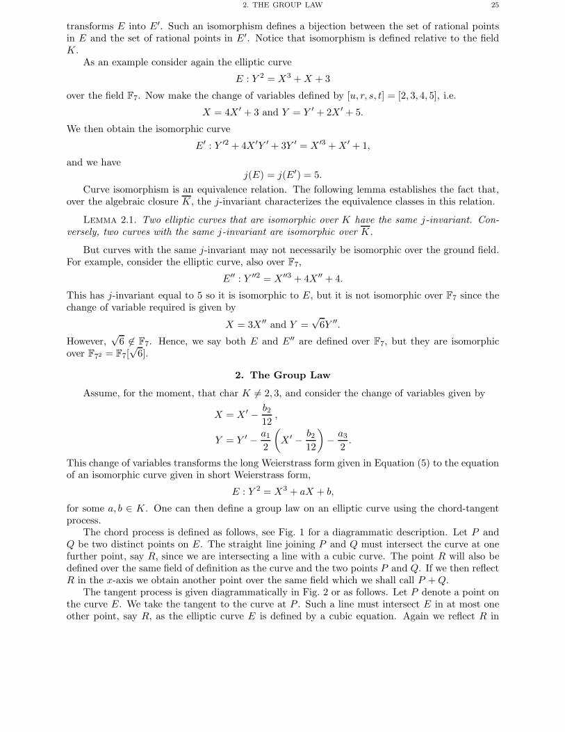
The chord process is defined as follows, see Fig. 1 for a diagrammatic description. Let P andQ be two distinct points on E. The straight line joining P and Q must intersect the curve at onefurther point, say R, since we are intersecting a line with a cubic curve. The point R will also bedefined over the same field of definition as the curve and the two points P and Q. If we then reflectR in the x-axis we obtain another point over the same field which we shall call P +Q.
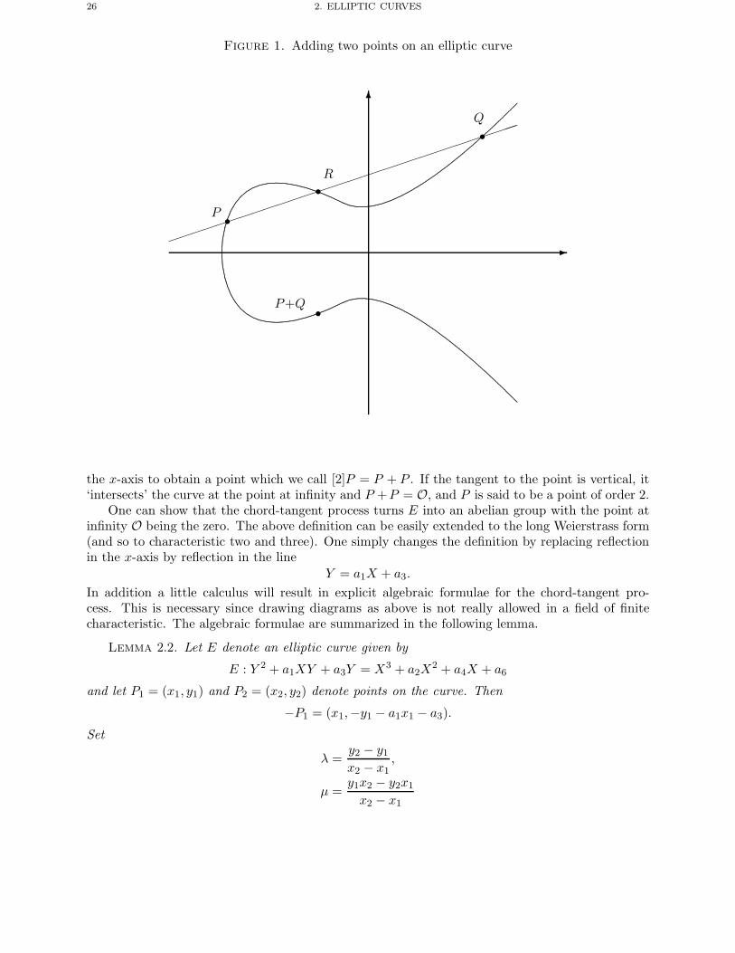
The tangent process is given diagrammatically in Fig. 2 or as follows. Let P denote a point onthe curve E. We take the tangent to the curve at P . Such a line must intersect E in at most oneother point, say R, as the elliptic curve E is defined by a cubic equation. Again we reflect R in
26 2. ELLIPTIC CURVES
Figure 1. Adding two points on an elliptic curve
.
.................................
..........
..........
..........
..
..........
..........
..........
..
.................................
.
..........................
........................
......................
....................
......................................
......................................... ...................... ........................ .......................... .............................
................................
...................................
.....................................
.
..........................
........................
......................
....................
...................
................... .................... ..................... ...................... ........................ .......................................................
...................................................................
.....................................
. ................... ................... .................... ...................... ..................................................
.............................
...............................
..................................
....................................
......................................
.........................................
...........................................
.............................................
................................................
..................................................
. ...................................... .................... ...................... ........................ ..........................
.............................
...............................
..................................
..................................
..
................................
......
..............................
...........
.............................
..............
............................
.................
..........................
......................
..........................
........................
������������������������������
�
�
P�
Q�
R�
P+Q�
the x-axis to obtain a point which we call [2]P = P + P . If the tangent to the point is vertical, it‘intersects’ the curve at the point at infinity and P +P = O, and P is said to be a point of order 2.
One can show that the chord-tangent process turns E into an abelian group with the point atinfinity O being the zero. The above definition can be easily extended to the long Weierstrass form(and so to characteristic two and three). One simply changes the definition by replacing reflectionin the x-axis by reflection in the line
Y = a1X + a3.
In addition a little calculus will result in explicit algebraic formulae for the chord-tangent pro-cess. This is necessary since drawing diagrams as above is not really allowed in a field of finitecharacteristic. The algebraic formulae are summarized in the following lemma.
Lemma 2.2. Let E denote an elliptic curve given by
E : Y 2 + a1XY + a3Y = X3 + a2X2 + a4X + a6
and let P1 = (x1, y1) and P2 = (x2, y2) denote points on the curve. Then
−P1 = (x1,−y1 − a1x1 − a3).
Set
λ =y2 − y1
x2 − x1,
μ =y1x2 − y2x1
x2 − x1
2. THE GROUP LAW 27
Figure 2. Doubling a point on an elliptic curve
.
.................................
..........
..........
..........
..
..........
..........
..........
..
.................................
.
..........................
........................
......................
....................
......................................
......................................... ...................... ........................ .......................... .............................
................................
...................................
.....................................
.
..........................
........................
......................
....................
...................
................... .................... ..................... ...................... ........................ .......................................................
...................................................................
.....................................
. ................... ................... .................... ...................... ..................................................
.............................
...............................
..................................
....................................
......................................
.........................................
...........................................
.............................................
................................................
..................................................
. ...................................... .................... ...................... ........................ ..........................
.............................
...............................
..................................
..................................
..
................................
......
..............................
...........
.............................
..............
............................
.................
..........................
......................
..........................
........................
��������������������������������
�
�
P�
R
�
[2]P�
when x1 �= x2, and set
λ =3x2
1 + 2a2x1 + a4 − a1y1
2y1 + a1x1 + a3,
μ =−x3
1 + a4x1 + 2a6 − a3y1
2y1 + a1x1 + a3
when x1 = x2 and P2 �= −P1. If
P3 = (x3, y3) = P1 + P2 �= Othen x3 and y3 are given by the formulae
x3 = λ2 + a1λ− a2 − x1 − x2,
y3 = −(λ+ a1)x3 − μ− a3.
The elliptic curve isomorphisms described earlier then become group isomorphisms as theyrespect the group structure.
For a positive integer m we let [m] denote the multiplication-by-m map from the curve to itself.This map takes a point P to
P + P + · · · + P,
where we have m summands. This map is the basis of elliptic curve cryptography, since whilst itis easy to compute, it is believed to be hard to invert, i.e. given P = (x, y) and [m]P = (x′, y′) it is
28 2. ELLIPTIC CURVES
hard to compute m. Of course this statement of hardness assumes a well-chosen elliptic curve etc.,something we will return to later in the book.
We end this section with an example of the elliptic curve group law. Again we take our ellipticcurve
E : Y 2 = X3 +X + 3
over the field F7. It turns out there are six points on this curve given by
O, (4, 1), (6, 6), (5, 0), (6, 1) and (4, 6).
These form a group with the group law being given by the following table, which is computed usingthe addition formulae given above.
+ O (4, 1) (6, 6) (5, 0) (6, 1) (4, 6)O O (4, 1) (6, 6) (5, 0) (6, 1) (4, 6)
(4, 1) (4, 1) (6, 6) (5, 0) (6, 1) (4, 6) O(6, 6) (6, 6) (5, 0) (6, 1) (4, 6) O (4, 1)(5, 0) (5, 0) (6, 1) (4, 6) O (4, 1) (6, 6)(6, 1) (6, 1) (4, 6) O (4, 1) (6, 6) (5, 0)(4, 6) (4, 6) O (4, 1) (6, 6) (5, 0) (6, 1)
As an example of the multiplication-by-m map, if we let
P = (4, 1)
then we have
[2]P = (6, 6),
[3]P = (5, 0),
[4]P = (6, 1),
[5]P = (4, 6),
[6]P = O.So we see in this example that E(F7) is a finite cyclic abelian group of order six generated by thepoint P . For all elliptic curves over finite fields the group is always finite and it is also highly likelyto be cyclic (or ‘nearly’ cyclic).
3. Elliptic Curves over Finite Fields
Over a finite field Fq, the number of rational points on a curve is finite, and its size will bedenoted by #E(Fq). The expected number of points on the curve is around q + 1 and if we set
#E(Fq) = q + 1 − t
then the value t is called the trace of Frobenius at q.A first approximation to the order of E(Fq) is given by the following well-known theorem of
Hasse.
Theorem 2.3 (H. Hasse, 1933). The trace of Frobenius satisfies
|t| ≤ 2√q.
Consider our example ofE : Y 2 = X3 +X + 3
then recall this has six points over the field F7, and so the associated trace of Frobenius is equal to2, which is less than 2
√q = 2
√7 = 5.29.
3. ELLIPTIC CURVES OVER FINITE FIELDS 29
The qth-power Frobenius map, on an elliptic curve E defined over Fq, is given by
ϕ :
⎧⎪⎨⎪⎩E(Fq) −→ E(Fq)(x, y) −→ (xq, yq)
O −→ O.The map ϕ sends points on E to points on E, no matter what the field of definition of the pointis. In addition the map ϕ respects the group law in that
ϕ(P +Q) = ϕ(P ) + ϕ(Q).
In other words the map ϕ is a group endomorphism of E over Fq, referred to as the Frobeniusendomorphism.
The trace of Frobenius t and the Frobenius endomorphism ϕ are linked by the equation
ϕ2 − [t]ϕ+ [q] = [0].
Hence, for any point P = (x, y) on the curve, we have
(xq2, yq
2) − [t](xq, yq) + [q](x, y) = O,
where addition and subtraction denote curve operations.
There are two particular classes of curves which, under certain conditions, will prove to becryptographically weak:
• The curve E(Fq) is said to be anomalous if its trace of Frobenius is one, giving #E(Fq) = q.These curves are weak when q = p, the field characteristic.
• The curve E(Fq) is said to be supersingular if the characteristic p divides the trace ofFrobenius, t. Such curves are usually considered weak cryptographically and are usuallyavoided. If q = p then this means that E(Fp) has p + 1 points since we must have t = 0.For other finite fields the possible values of t corresponding to supersingular elliptic curvesare given by, where q = pf ,
• f odd: t = 0, t2 = 2q and t2 = 3q.• f even : t2 = 4q, t2 = q if p = 1 (mod 3) and t = 0 if p �= 1 (mod 4).
We will also need to choose a curve such that the group order #E(Fq) is divisible by a large primenumber. This means we need to be able to compute the group order #E(Fq), so as to check boththis and the above two conditions.
For any elliptic curve and any finite field the group order #E(Fq) can be computed in polynomialtime. But this is usually done via a complicated algorithm that we cannot go into in this book.Hence, you should just remember that computing the group order is easy. We shall see in a laterchapter, when considering algorithms to solve discrete logarithm problems, that knowing the grouporder is important in understanding how secure a group is.
One of the advantages of elliptic curves is that there is a very large number of possible groups.One can choose both the finite field and the coefficients of the curve. In addition finding ellipticcurves with the correct cryptographic properties to make them secure is relatively easy.
As was apparent from the earlier discussion, the cases char K = 2, 3 often require separatetreatment. Practical implementations of elliptic curve cryptosystems are usually based on eitherF2n , i.e. characteristic two, or Fp for large primes p. Therefore, in the remainder of this chapterwe will focus on fields of characteristic two and p > 3, and will omit the separate treatment of thecase char K = 3. Most arguments, though, carry easily to characteristic three, with modificationsthat are well documented in the literature.
30 2. ELLIPTIC CURVES
3.1. Curves over Fields of Characteristic p > 3. Assume that our finite field is given byK = Fq, where q = pn for a prime p > 3 and an integer n ≥ 1. As mentioned, the curve equationin this case can be simplified to the short Weierstrass form
E : Y 2 = X3 + aX + b.
The discriminant of the curve then reduces to Δ = −16(4a3 + 27b2), and its j-invariant to j(E) =−1728(4a)3/Δ. The formulae for the group law in Lemma 2.2 also simplify to
−P1 = (x1,−y1),
and ifP3 = (x3, y3) = P1 + P2 �= O,
then x3 and y3 are given by the formulae
x3 = λ2 − x1 − x2,
y3 = (x1 − x3)λ− y1,
where if x1 �= x2 we set
λ =y2 − y1
x2 − x1,
and if x1 = x2, y1 �= 0 we set
λ =3x2
1 + a
2y1.
3.2. Curves over Fields of Characteristic Two. We now specialize to the case of finitefields where q = 2n with n ≥ 1. In this case, the expression for the j-invariant reduces to j(E) =a12
1 /Δ. In characteristic two, the condition j(E) = 0, i.e. a1 = 0, is equivalent to the curve beingsupersingular. As mentioned earlier, this very special type of curve is avoided in cryptography. Weassume, therefore, that j(E) �= 0.
Under these assumptions, a representative for each isomorphism class of elliptic curves over Fqis given by
(6) E : Y 2 +XY = X3 + a2X2 + a6,
where a6 ∈ F∗q and a2 ∈ {0, γ} with γ a fixed element in Fq such that Trq|2(γ) = 1, where Trq|2 is
the absolute trace
Tr2n|2(α) =n−1∑i=0
α2i .
The formulae for the group law in Lemma 2.2 then simplify to
−P1 = (x1, y1 + x1),
and ifP3 = (x3, y3) = P1 + P2 �= O,
then x3 and y3 are given by the formulae
x3 = λ2 + λ+ a2 + x1 + x2,
y3 = (λ+ 1)x3 + μ
= (x1 + x3)λ+ x3 + y1,
where if x1 �= x2 we set
λ =y2 + y1
x2 + x1,
μ =y1x2 + y2x1
x2 + x1
4. PROJECTIVE COORDINATES 31
and if x1 = x2 �= 0 we set
λ =x2
1 + y1
x1,
μ = x21.
4. Projective Coordinates
One of the problems with the above formulae for the group laws given in both large and evencharacteristic is that at some stage they involve a division operation. Division in finite fieldsis considered as an expensive operation, since it usually involves some variant of the extendedEuclidean algorithm, which although of approximately the same complexity as multiplication canusually not be implemented as efficiently.
To avoid these division operations one can use projective coordinates. Here one writes theelliptic curve using three variables (X,Y,Z) instead of just (X,Y ). Instead of using the projectiverepresentation given at the start of this chapter we instead use one where the curve is written as
E : Y 2 + a1XY Z + a2Y Z4 = X3 + a2X
2Z2 + a4XZ4 + a6Z
6.
The point at infinity is still denoted by (0, 1, 0), but now the map from projective to affine coordi-nates is given by
(X,Y,Z) −→ (X/Z2, Y/Z3).
This choice of projective coordinates is made to provide a more efficient arithmetic operation.
4.1. Large Prime Characteristic. The formulae for point addition when our elliptic curveis written as
Y 2 = X3 + aXZ4 + bZ6
are now given by the law
(X3, Y3, Z3) = (X1, Y1, Z1) + (X2, Y2, Z2)
where (X3, Y3, Z3) are derived from the formulae
λ1 = X1Z22 , λ2 = X2Z
21 ,
λ3 = λ1 − λ2, λ4 = Y1Z32 ,
λ5 = Y2Z31 , λ6 = λ4 − λ5,
λ7 = λ1 + λ2, λ8 = λ4 + λ5,
Z3 = Z1Z2λ3, X3 = λ26 − λ7λ
23,
λ9 = λ7λ23 − 2X3, Y3 = (λ9λ6 − λ8λ
33)/2.
Notice the avoidance of any division operation, bar division by 2 which can be easily accomplishedby multiplication of the precomputed value of 2−1 (mod p).
Doubling a point,(X3, Y3, Z3) = [2](X1, Y1, Z1),
can be accomplished using the formulae
λ1 = 3X21 + aZ4
1 , Z3 = 2Y1Z1,
λ2 = 4X1Y21 , X3 = λ2
1 − 2λ2,
λ3 = 8Y 41 , Y3 = λ1(λ2 −X3) − λ3.
32 2. ELLIPTIC CURVES
4.2. Even Characteristic. In even characteristic we write our elliptic curve in the form
Y 2 +XY Z = X3 + a2X2Z2 + a6Z
6.
Point addition,
(X3, Y3, Z3) = (X1, Y1, Z1) + (X2, Y2, Z2)
is now accomplished using the recipe
λ1 = X1Z22 , λ2 = X2Z
21 ,
λ3 = λ1 + λ2, λ4 = Y1Z32 ,
λ5 = Y2Z31 , λ6 = λ4 + λ5,
λ7 = Z1λ3, λ8 = λ6X2 + λ7Y2,
Z3 = λ7Z2, λ9 = λ6 + Z3,
X3 = a2Z23 + λ6λ9 + λ3
3, Y3 = λ9X3 + λ8λ27.
Doubling is then performed using
Z3 = X1Z21 , X3 = (X1 + d6Z
21 )4,
λ = Z3 +X21 + Y1Z1, Y3 = X4
1Z3 + λX3,
where d6 = 4√a6.
Notice how in both even and odd characteristic we have avoided a division operation.
5. Point Compression
In many cryptographic protocols we need to store or transmit an elliptic curve point. Usingaffine coordinates this can be accomplished using two field elements, i.e. by transmitting x andthen y. However, one can do better using a technique called point compression.
Point compression works by the observation that for every x-coordinate on the curve there are atmost two corresponding y-coordinates. Hence, we can represent a point by storing the x-coordinatealong with a bit b to say which value of the y-coordinate we should take. All that remains to decideis how to compute the bit b and how to reconstruct the y-coordinate given the x-coordinate andthe bit b.
5.1. Large Prime Characteristic. For elliptic curves over fields of large prime characteristicwe notice that if α ∈ F∗
p then the two square roots ±β of α have different parities, when representedas integers in the range [1, . . . , p− 1]. This is because
−β = p− β.
Hence, as the bit b we choose the parity of the y-coordinate.Then, given (x, b), we can reconstruct y by computing
β =√x3 + ax+ b (mod p).
If the parity of β is equal to b we set y = β, otherwise we set y = p − β. If β = 0 then no matterwhich value of b we have we set y = 0.

Chapter Summary 33
5.2. Even Characteristic. In even characteristic we need to be slightly more clever. Supposewe are given a point P = (x, y) on the elliptic curve
Y 2 +XY = X3 + a2X + a6.
If y = 0 then we set b = 0, otherwise we compute
z = y/x
and let b denote the least significant bit of z. To recover y given (x, b), for x �= 0, we set
α = x+ a2 +a6
x2
and let β denote a solution ofz2 + z = α.
Then if the least significant bit of β is equal to b we set y = xβ, otherwise we set y = x(β + 1). Tosee why this works notice that if (x, y) is a solution of
Y 2 +XY = X3 + a2X2 + a6
then (x, y/x) and (x, 1 + y/x) are the two solutions of
Z2 + Z = X + a2 +a6
X2.
As an example consider the curve
E : Y 2 = X3 +X + 3
over the field F7. Then the points (4, 1) and (4, 6) which in bits we need to represent as
(0b100, 0b001) and (0b100, 0b110),
i.e. requiring six bits for each point, can be represented as
(0b100, 0b1) and (0b100, 0b0),
where we only use four bits for each point.In larger, cryptographically interesting, examples the advantage becomes more pronounced.
For example consider the same curve over the field
p = 1125 899 906 842 679 = 250 + 55
then the point(1 125 899 906 842 675, 245 132 605 757 739)
can be represented by the integers
(1 125 899 906 842 675, 1).
So instead of requiring 102 bits we only require 52 bits.
Chapter Summary
• Elliptic curves over finite fields are another example of a finite abelian group. There are alot of such groups since we are free to choose both the curve and the field.
• For cryptography we need to be able to compute the number of elements in the group.Although this is done using a complicated algorithm, it can be done in polynomial time.
34 2. ELLIPTIC CURVES
• One should usually avoid supersingular and anomalous curves in cryptographic applica-tions.
• Efficient algorithms for the group law can be produced by using projective coordinates.These algorithms avoid the need for costly division operations in the underlying finite field.
• To save bandwidth and space it is possible to efficiently compress elliptic curve points(x, y) down to x and a single bit b. The uncompression can also be performed efficiently.
Further Reading
For those who wish to learn more about elliptic curves in general try the textbook by Silverman(which is really aimed at mathematics graduate students). For those who are simply interested inthe cryptographic applications of elliptic curves and the associated algorithms and techniques seethe book by Blake, Seroussi and Smart.
I.F. Blake, G. Seroussi and N.P. Smart. Elliptic Curves in Cryptography. Cambridge UniversityPress, 1999.
J.H. Silverman. The Arithmetic of Elliptic Curves. Springer-Verlag, 1985.
Part 2
Symmetric Encryption
Encryption of most data is accomplished using fast block and stream ciphers. These are ex-amples of symmetric encryption algorithms. In addition all historical, i.e. pre-1960, ciphers aresymmetric in nature and share some design principles with modern ciphers.
The main drawback with symmetric ciphers is that they give rise to a problem of how todistribute the secret keys between users, so we also address this issue.
We also discuss the properties and design of cryptographic hash functions and message authen-tication codes. Both of which will form basic building blocks of other schemes and protocols withinthis book.
In the following chapters we explain the theory and practice of modern symmetric ciphers, butfirst we consider historical ciphers.

CHAPTER 3
Historical Ciphers
Chapter Goals
• To explain a number of historical ciphers, such as the Caesar cipher, substitution cipher.• To show how these historical ciphers can be broken because they do not hide the underlying
statistics of the plaintext.• To introduce the concepts of substitution and permutation as basic cipher components.• To introduce a number of attack techniques, such as chosen plaintext attacks.
1. Introduction
An encryption algorithm, or cipher, is a means of transforming plaintext into ciphertext underthe control of a secret key. This process is called encryption or encipherment. We write
c = ek(m),
where• m is the plaintext,• e is the cipher function,• k is the secret key,• c is the ciphertext.
The reverse process is called decryption or decipherment, and we write
m = dk(c).
Note, that the encryption and decryption algorithms e, d are public, the secrecy of m given cdepends totally on the secrecy of k.
The above process requires that each party needs access to the secret key. This needs to beknown to both sides, but needs to be kept secret. Encryption algorithms which have this propertyare called symmetric cryptosystems or secret key cryptosystems. There is a form of cryptographywhich uses two different types of key, one is publicly available and used for encryption whilst theother is private and used for decryption. These latter types of cryptosystems are called asymmetriccryptosystems or public key cryptosystems, to which we shall return in a later chapter.
Usually in cryptography the communicating parties are denoted by A and B. However, oftenone uses the more user-friendly names of Alice and Bob. But you should not assume that theparties are necessarily human, we could be describing a communication being carried out betweentwo autonomous machines. The eavesdropper, bad girl, adversary or attacker is usually given thename Eve.
In this chapter we shall present some historical ciphers which were used in the pre-computerage to encrypt data. We shall show that these ciphers are easy to break as soon as one understandsthe statistics of the underlying language, in our case English. In Chapter 5 we shall study thisrelationship between how easy the cipher is to break and the statistical distribution of the underlyingplaintext.
37
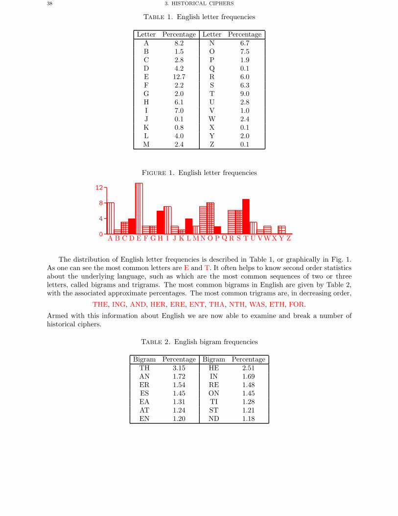
38 3. HISTORICAL CIPHERS
Table 1. English letter frequencies
Letter Percentage Letter PercentageA 8.2 N 6.7B 1.5 O 7.5C 2.8 P 1.9D 4.2 Q 0.1E 12.7 R 6.0F 2.2 S 6.3G 2.0 T 9.0H 6.1 U 2.8I 7.0 V 1.0J 0.1 W 2.4K 0.8 X 0.1L 4.0 Y 2.0M 2.4 Z 0.1
Figure 1. English letter frequencies
0
4
8
12
A B C D E F G H I J K L MN O P Q R S T U VWX Y Z
The distribution of English letter frequencies is described in Table 1, or graphically in Fig. 1.As one can see the most common letters are E and T. It often helps to know second order statisticsabout the underlying language, such as which are the most common sequences of two or threeletters, called bigrams and trigrams. The most common bigrams in English are given by Table 2,with the associated approximate percentages. The most common trigrams are, in decreasing order,
THE, ING, AND, HER, ERE, ENT, THA, NTH, WAS, ETH, FOR.
Armed with this information about English we are now able to examine and break a number ofhistorical ciphers.
Table 2. English bigram frequencies
Bigram Percentage Bigram PercentageTH 3.15 HE 2.51AN 1.72 IN 1.69ER 1.54 RE 1.48ES 1.45 ON 1.45EA 1.31 TI 1.28AT 1.24 ST 1.21EN 1.20 ND 1.18
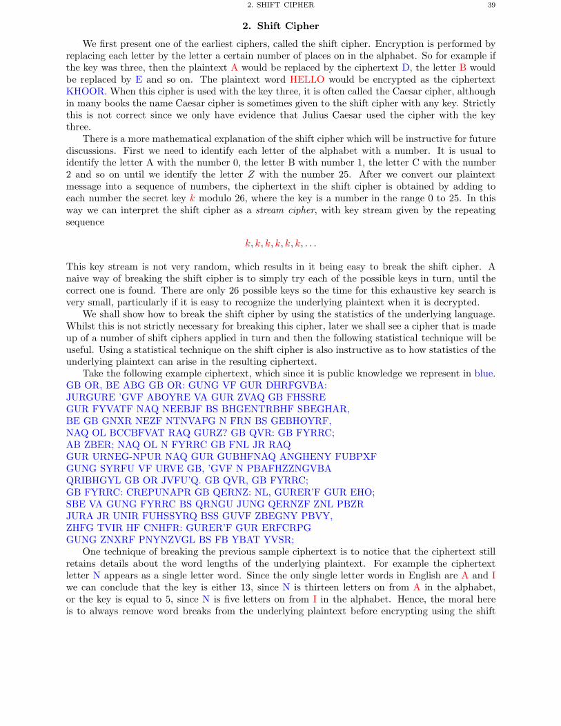
2. SHIFT CIPHER 39
2. Shift Cipher
We first present one of the earliest ciphers, called the shift cipher. Encryption is performed byreplacing each letter by the letter a certain number of places on in the alphabet. So for example ifthe key was three, then the plaintext A would be replaced by the ciphertext D, the letter B wouldbe replaced by E and so on. The plaintext word HELLO would be encrypted as the ciphertextKHOOR. When this cipher is used with the key three, it is often called the Caesar cipher, althoughin many books the name Caesar cipher is sometimes given to the shift cipher with any key. Strictlythis is not correct since we only have evidence that Julius Caesar used the cipher with the keythree.
There is a more mathematical explanation of the shift cipher which will be instructive for futurediscussions. First we need to identify each letter of the alphabet with a number. It is usual toidentify the letter A with the number 0, the letter B with number 1, the letter C with the number2 and so on until we identify the letter Z with the number 25. After we convert our plaintextmessage into a sequence of numbers, the ciphertext in the shift cipher is obtained by adding toeach number the secret key k modulo 26, where the key is a number in the range 0 to 25. In thisway we can interpret the shift cipher as a stream cipher, with key stream given by the repeatingsequence
k, k, k, k, k, k, . . .
This key stream is not very random, which results in it being easy to break the shift cipher. Anaive way of breaking the shift cipher is to simply try each of the possible keys in turn, until thecorrect one is found. There are only 26 possible keys so the time for this exhaustive key search isvery small, particularly if it is easy to recognize the underlying plaintext when it is decrypted.
We shall show how to break the shift cipher by using the statistics of the underlying language.Whilst this is not strictly necessary for breaking this cipher, later we shall see a cipher that is madeup of a number of shift ciphers applied in turn and then the following statistical technique will beuseful. Using a statistical technique on the shift cipher is also instructive as to how statistics of theunderlying plaintext can arise in the resulting ciphertext.
Take the following example ciphertext, which since it is public knowledge we represent in blue.GB OR, BE ABG GB OR: GUNG VF GUR DHRFGVBA:JURGURE ’GVF ABOYRE VA GUR ZVAQ GB FHSSREGUR FYVATF NAQ NEEBJF BS BHGENTRBHF SBEGHAR,BE GB GNXR NEZF NTNVAFG N FRN BS GEBHOYRF,NAQ OL BCCBFVAT RAQ GURZ? GB QVR: GB FYRRC;AB ZBER; NAQ OL N FYRRC GB FNL JR RAQGUR URNEG-NPUR NAQ GUR GUBHFNAQ ANGHENY FUBPXFGUNG SYRFU VF URVE GB, ’GVF N PBAFHZZNGVBAQRIBHGYL GB OR JVFU’Q. GB QVR, GB FYRRC;GB FYRRC: CREPUNAPR GB QERNZ: NL, GURER’F GUR EHO;SBE VA GUNG FYRRC BS QRNGU JUNG QERNZF ZNL PBZRJURA JR UNIR FUHSSYRQ BSS GUVF ZBEGNY PBVY,ZHFG TVIR HF CNHFR: GURER’F GUR ERFCRPGGUNG ZNXRF PNYNZVGL BS FB YBAT YVSR;
One technique of breaking the previous sample ciphertext is to notice that the ciphertext stillretains details about the word lengths of the underlying plaintext. For example the ciphertextletter N appears as a single letter word. Since the only single letter words in English are A and Iwe can conclude that the key is either 13, since N is thirteen letters on from A in the alphabet,or the key is equal to 5, since N is five letters on from I in the alphabet. Hence, the moral hereis to always remove word breaks from the underlying plaintext before encrypting using the shift
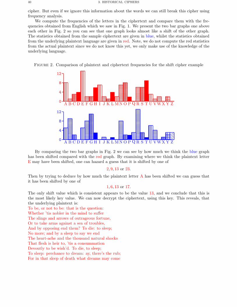
40 3. HISTORICAL CIPHERS
cipher. But even if we ignore this information about the words we can still break this cipher usingfrequency analysis.
We compute the frequencies of the letters in the ciphertext and compare them with the fre-quencies obtained from English which we saw in Fig. 1. We present the two bar graphs one aboveeach other in Fig. 2 so you can see that one graph looks almost like a shift of the other graph.The statistics obtained from the sample ciphertext are given in blue, whilst the statistics obtainedfrom the underlying plaintext language are given in red. Note, we do not compute the red statisticsfrom the actual plaintext since we do not know this yet, we only make use of the knowledge of theunderlying language.
Figure 2. Comparison of plaintext and ciphertext frequencies for the shift cipher example
0
4
8
12
A B C D E F G H I J K L MN O P Q R S T U VWX Y Z
0
4
8
12
A B C D E F G H I J K L MN O P Q R S T U VWX Y��������
Z
By comparing the two bar graphs in Fig. 2 we can see by how much we think the blue graphhas been shifted compared with the red graph. By examining where we think the plaintext letterE may have been shifted, one can hazard a guess that it is shifted by one of
2, 9, 13 or 23.
Then by trying to deduce by how much the plaintext letter A has been shifted we can guess thatit has been shifted by one of
1, 6, 13 or 17.The only shift value which is consistent appears to be the value 13, and we conclude that this isthe most likely key value. We can now decrypt the ciphertext, using this key. This reveals, thatthe underlying plaintext is:To be, or not to be: that is the question:Whether ’tis nobler in the mind to sufferThe slings and arrows of outrageous fortune,Or to take arms against a sea of troubles,And by opposing end them? To die: to sleep;No more; and by a sleep to say we endThe heart-ache and the thousand natural shocksThat flesh is heir to, ’tis a consummationDevoutly to be wish’d. To die, to sleep;To sleep: perchance to dream: ay, there’s the rub;For in that sleep of death what dreams may come
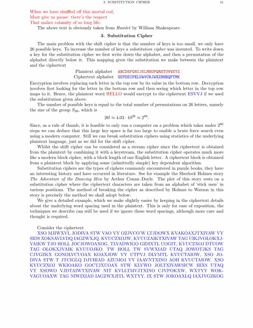
3. SUBSTITUTION CIPHER 41
When we have shuffled off this mortal coil,Must give us pause: there’s the respectThat makes calamity of so long life;
The above text is obviously taken from Hamlet by William Shakespeare.
3. Substitution Cipher
The main problem with the shift cipher is that the number of keys is too small, we only have26 possible keys. To increase the number of keys a substitution cipher was invented. To write downa key for the substitution cipher we first write down the alphabet, and then a permutation of thealphabet directly below it. This mapping gives the substitution we make between the plaintextand the ciphertext
Plaintext alphabet ABCDEFGHIJKLMNOPQRSTUVWXYZCiphertext alphabet GOYDSIPELUAVCRJWXZNHBQFTMK
Encryption involves replacing each letter in the top row by its value in the bottom row. Decryptioninvolves first looking for the letter in the bottom row and then seeing which letter in the top rowmaps to it. Hence, the plaintext word HELLO would encrypt to the ciphertext ESVVJ if we usedthe substitution given above.
The number of possible keys is equal to the total number of permutations on 26 letters, namelythe size of the group S26, which is
26! ≈ 4.03 · 1026 ≈ 288.
Since, as a rule of thumb, it is feasible to only run a computer on a problem which takes under 280
steps we can deduce that this large key space is far too large to enable a brute force search evenusing a modern computer. Still we can break substitution ciphers using statistics of the underlyingplaintext language, just as we did for the shift cipher.
Whilst the shift cipher can be considered as a stream cipher since the ciphertext is obtainedfrom the plaintext by combining it with a keystream, the substitution cipher operates much morelike a modern block cipher, with a block length of one English letter. A ciphertext block is obtainedfrom a plaintext block by applying some (admittedly simple) key dependent algorithm.
Substitution ciphers are the types of ciphers commonly encountered in puzzle books, they havean interesting history and have occurred in literature. See for example the Sherlock Holmes storyThe Adventure of the Dancing Men by Arthur Conan–Doyle. The plot of this story rests on asubstitution cipher where the ciphertext characters are taken from an alphabet of ‘stick men’ invarious positions. The method of breaking the cipher as described by Holmes to Watson in thisstory is precisely the method we shall adopt below.
We give a detailed example, which we make slightly easier by keeping in the ciphertext detailsabout the underlying word spacing used in the plaintext. This is only for ease of exposition, thetechniques we describe can still be used if we ignore these word spacings, although more care andthought is required.
Consider the ciphertextXSO MJIWXVL JODIVA STW VAO VY OZJVCO’W LTJDOWX KVAKOAXJTXIVAW VY
SIDS XOKSAVLVDQ IAGZWXJQ. KVUCZXOJW, KVUUZAIKTXIVAW TAG UIKJVOLOKXJ-VAIKW TJO HOLL JOCJOWOAXOG, TLVADWIGO GIDIXTL UOGIT, KVUCZXOJ DTUOWTAG OLOKXJVAIK KVUUOJKO. TW HOLL TW SVWXIAD UTAQ JOWOTJKS TAGCJVGZKX GONOLVCUOAX KOAXJOW VY UTPVJ DLVMTL KVUCTAIOW, XSO JO-DIVA STW T JTCIGLQ DJVHIAD AZUMOJ VY IAAVNTXINO AOH KVUCTAIOW. XSOKVUCZXOJ WKIOAKO GOCTJXUOAX STW KLVWO JOLTXIVAWSICW HIXS UTAQVY XSOWO VJDTAIWTXIVAW NIT KVLLTMVJTXINO CJVPOKXW, WXTYY WOK-VAGUOAXW TAG NIWIXIAD IAGZWXJITL WXTYY. IX STW JOKOAXLQ IAXJVGZKOG
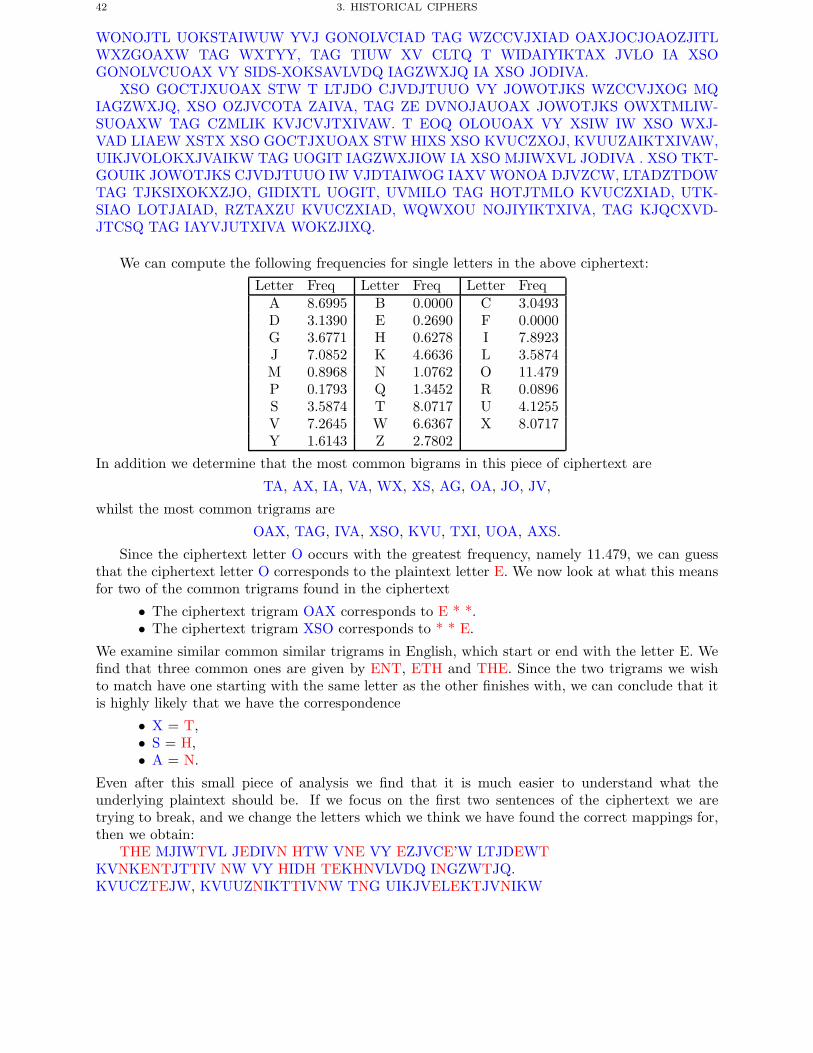
42 3. HISTORICAL CIPHERS
WONOJTL UOKSTAIWUW YVJ GONOLVCIAD TAG WZCCVJXIAD OAXJOCJOAOZJITLWXZGOAXW TAG WXTYY, TAG TIUW XV CLTQ T WIDAIYIKTAX JVLO IA XSOGONOLVCUOAX VY SIDS-XOKSAVLVDQ IAGZWXJQ IA XSO JODIVA.
XSO GOCTJXUOAX STW T LTJDO CJVDJTUUO VY JOWOTJKS WZCCVJXOG MQIAGZWXJQ, XSO OZJVCOTA ZAIVA, TAG ZE DVNOJAUOAX JOWOTJKS OWXTMLIW-SUOAXW TAG CZMLIK KVJCVJTXIVAW. T EOQ OLOUOAX VY XSIW IW XSO WXJ-VAD LIAEW XSTX XSO GOCTJXUOAX STW HIXS XSO KVUCZXOJ, KVUUZAIKTXIVAW,UIKJVOLOKXJVAIKW TAG UOGIT IAGZWXJIOW IA XSO MJIWXVL JODIVA . XSO TKT-GOUIK JOWOTJKS CJVDJTUUO IW VJDTAIWOG IAXV WONOA DJVZCW, LTADZTDOWTAG TJKSIXOKXZJO, GIDIXTL UOGIT, UVMILO TAG HOTJTMLO KVUCZXIAD, UTK-SIAO LOTJAIAD, RZTAXZU KVUCZXIAD, WQWXOU NOJIYIKTXIVA, TAG KJQCXVD-JTCSQ TAG IAYVJUTXIVA WOKZJIXQ.
We can compute the following frequencies for single letters in the above ciphertext:
Letter Freq Letter Freq Letter FreqA 8.6995 B 0.0000 C 3.0493D 3.1390 E 0.2690 F 0.0000G 3.6771 H 0.6278 I 7.8923J 7.0852 K 4.6636 L 3.5874M 0.8968 N 1.0762 O 11.479P 0.1793 Q 1.3452 R 0.0896S 3.5874 T 8.0717 U 4.1255V 7.2645 W 6.6367 X 8.0717Y 1.6143 Z 2.7802
In addition we determine that the most common bigrams in this piece of ciphertext are
TA, AX, IA, VA, WX, XS, AG, OA, JO, JV,
whilst the most common trigrams are
OAX, TAG, IVA, XSO, KVU, TXI, UOA, AXS.
Since the ciphertext letter O occurs with the greatest frequency, namely 11.479, we can guessthat the ciphertext letter O corresponds to the plaintext letter E. We now look at what this meansfor two of the common trigrams found in the ciphertext
• The ciphertext trigram OAX corresponds to E * *.• The ciphertext trigram XSO corresponds to * * E.
We examine similar common similar trigrams in English, which start or end with the letter E. Wefind that three common ones are given by ENT, ETH and THE. Since the two trigrams we wishto match have one starting with the same letter as the other finishes with, we can conclude that itis highly likely that we have the correspondence
• X = T,• S = H,• A = N.
Even after this small piece of analysis we find that it is much easier to understand what theunderlying plaintext should be. If we focus on the first two sentences of the ciphertext we aretrying to break, and we change the letters which we think we have found the correct mappings for,then we obtain:
THE MJIWTVL JEDIVN HTW VNE VY EZJVCE’W LTJDEWTKVNKENTJTTIV NW VY HIDH TEKHNVLVDQ INGZWTJQ.KVUCZTEJW, KVUUZNIKTTIVNW TNG UIKJVELEKTJVNIKW
3. SUBSTITUTION CIPHER 43
TJE HELL JECJEWENTEG, TLVNDWIGE GIDITTL UEGIT,KVUCZTEJ DTUEW TNG ELEKTJVNIK KVUUEJKE.
Recall, this was after the four substitutionsO = E, X = T, S = H, A = N.
We now cheat and use the fact that we have retained the word sizes in the ciphertext. We see thatsince the letter T occurs as a single ciphertext letter we must have
T = I or T = A.The ciphertext letter T occurs with a probability of 8.0717, which is the highest probability left,hence we are far more likely to have
T = A.We have already considered the most popular trigram in the ciphertext so turning our attentionto the next most popular trigram we see that it is equal to TAG which we suspect corresponds tothe plaintext AN*. Therefore it is highly likely that G = D, since AND is a popular trigram inEnglish.
Our partially decrypted ciphertext is now equal toTHE MJIWTVL JEDIVN HAW VNE VY EZJVCE’W LAJDEWT
KVNKENTJATIV NW VY HIDH TEKHNVLVDQ INDZWTJQ.KVUCZTEJW, KVUUZNIKATIVNW AND UIKJVELEKTJVNIKWAJE HELL JECJEWENTED, ALVNDWIDE DIDITAL UEDIA,KVUCZTEJ DAUEW AND ELEKTJVNIK KVUUEJKE.
This was after the six substitutionsO = E, X = T, S = H,A = N, T = A, G = D.
We now look at two-letter words which occur in the ciphertext:• IX
This corresponds to the plaintext *T. Therefore the ciphertext letter I must be one of theplaintext letters A or I, since the only two-letter words in English ending in T are AT andIT. We already have worked out what the plaintext character A corresponds to, hence wemust have I = I.
• XVThis corresponds to the plaintext T*. Hence, we must have V = O.
• VYThis corresponds to the plaintext O*. Hence, the ciphertext letter Y must correspondto one of F, N or R. We already know the ciphertext letter corresponding to N. In theciphertext the probability of Y occurring is 1.6, but in English we expect F to occur withprobability 2.2 and R to occur with probability 6.0. Hence, it is more likely that Y = F.
• IWThis corresponds to the plaintext I*. Therefore, the plaintext character W must be oneof F, N, S and T. We already have F, N, T, hence W = S.
All these deductions leave the partial ciphertext asTHE MJISTOL JEDION HAS ONE OF EZJOCE’S LAJDEST
KONKENTJATIONS OF HIDH TEKHNOLODQ INDZSTJQ.KOUCZTEJS, KOUUZNIKATIONS AND UIKJOELEKTJONIKS AJEHELL JECJESENTED, ALONDSIDE DIDITAL UEDIA,KOUCZTEJ DAUES AND ELEKTJONIK KOUUEJKE.
This was after the ten substitutionsO = E, X = T, S = H, A = N, T = A,G = D, I = I, V = O, Y = F, W = S.
44 3. HISTORICAL CIPHERS
Even with half the ciphertext letters determined it is now quite easy to understand the underlyingplaintext, taken from the website of the University of Bristol Computer Science Department. Weleave it to the reader to determine the final substitutions and recover the plaintext completely.
4. Vigenere Cipher
The problem with the shift cipher and the substitution cipher was that each plaintext letteralways encrypted to the same ciphertext letter. Hence underlying statistics of the language could beused to break the cipher. For example it was easy to determine which ciphertext letter correspondedto the plaintext letter E. From the early 1800s onwards, cipher designers tried to break this linkbetween the plaintext and ciphertext.
The substitution cipher we used above was a mono-alphabetic substitution cipher, in that onlyone alphabet substitution was used to encrypt the whole alphabet. One way to solve our problem isto take a number of substitution alphabets and then encrypt each letter with a different alphabet.Such a system is called a polyalphabetic substitution cipher.
For example we could takePlaintext alphabet ABCDEFGHIJKLMNOPQRSTUVWXYZCiphertext alphabet one TMKGOYDSIPELUAVCRJWXZNHBQFCiphertext alphabet two DCBAHGFEMLKJIZYXWVUTSRQPON
Then the plaintext letters in an odd position we encrypt using the first ciphertext alphabet, whilstthe plaintext letters in even positions we encrypt using the second alphabet. For example theplaintext word HELLO, using the above alphabets would encrypt to SHLJV. Notice that the twooccurrences of L in the plaintext encrypt to two different ciphertext characters. Thus we havemade it harder to use the underlying statistics of the language. If one now does a naive frequencyanalysis we no longer get a common ciphertext letter corresponding to the plaintext letter E.
We essentially are encrypting the message two letters at a time, hence we have a block cipherwith block length two English characters. In real life one may wish to use around five rather thanjust two alphabets and the resulting key becomes very large indeed. With five alphabets the totalkey space is
(26!)5 ≈ 2441,
but the user only needs to remember the key which is a sequence of
26 · 5 = 130
letters. However, just to make life hard for the attacker, the number of alphabets in use shouldalso be hidden from his view and form part of the key. But for the average user in the early 1800sthis was far too unwieldy a system, since the key was too hard to remember.
Despite its shortcomings the most famous cipher during the 19th-century was based on preciselythis principle. The Vigenere cipher, invented in 1533 by Giovan Batista Belaso, was a variant onthe above theme, but the key was easy to remember. When looked at in one way the Vigenerecipher is a polyalphabetic block cipher, but when looked at in another, it is a stream cipher whichis a natural generalization of the shift cipher.
The description of the Vigenere cipher as a block cipher takes the description of the polyal-phabetic cipher above but restricts the possible plaintext alphabets to one of the 26 possible cyclicshifts of the standard alphabet. Suppose five alphabets were used, this reduces the key space downto
265 ≈ 223
and the size of the key to be remembered as a sequence of five numbers between 0 and 25.However, the description of the Vigenere cipher as a stream cipher is much more natural. Just
like the shift cipher, the Vigenere cipher again identifies letters with the numbers 0, . . . , 25. Thesecret key is a short sequence of letters (e.g. a word) which is repeated again and again to form
4. VIGENERE CIPHER 45
a keystream. Encryption involves adding the plaintext letter to a key letter. Thus if the key isSESAME, encryption works as follows,
THISISATESTMESSAGESESAMESESAMESESAMELLASUWSXWSFQWWKASI
Again we notice that A will encrypt to a different letter depending on where it appears in themessage.
But the Vigenere cipher is still easy to break using the underlying statistics of English. Oncewe have found the length of the keyword, breaking the ciphertext is the same as breaking the shiftcipher a number of times.
As an example, suppose the ciphertext is given byUTPDHUG NYH USVKCG MVCE FXL KQIB. WX RKU GI TZN, RLS BBHZLXMSNP
KDKS; CEB IH HKEW IBA, YYM SBR PFR SBS, JV UPL O UVADGR HRRWXF. JV ZTVOOVYH ZCQU Y UKWGEB, PL UQFB P FOUKCG, TBF RQ VHCF R KPG, OU KFT ZCQU MAWQKKW ZGSY, FP PGM QKFTK UQFB DER EZRN, MCYE, MG UCTFSVA, WP KFT ZCQUMAW KQIJS. LCOV NTHDNV JPNUJVB IH GGV RWX ONKCGTHKFL XG VKD, ZJM VGCCI MVGD JPNUJ, RLS EWVKJT ASGUCS MVGD; DDK VG NYH PWUV CCHIIY RD DBQNRWTH PFRWBBI VTTK VCGNTGSF FL IAWU XJDUS, HFP VHCF, RR LAWEY QDFSRVMEES FZB CHH JRTT MVGZP UBZN FD ATIIYRTK WP KFT HIVJCI; TBF BLDPWPXRWTH ULAW TG VYCHX KQLJS US DCGCW OPPUPR, VG KFDNUJK GI JIKKC PL KGCJIAOV KFTR GJFSAW KTZLZES WG RWXWT VWTL WP XPXGG, CJ FPOS VYC BTZCUWXG ZGJQ PMHTRAIBJG WMGFG. JZQ DPB JVYGM ZCLEWXR: CEB IAOV NYH JIKKCTGCWXF UHF JZK.
WX VCU LD YITKFTK WPKCGVCWIQT PWVY QEBFKKQ, QNH NZTTW IRFL IASVFRPE ODJRXGSPTC EKWPTGEES, GMCGTTVVPLTFFJ; YCW WV NYH TZYRWH LOKU MU AWO, KFPM VG BLTP VQN RD DSGGAWKWUKKPL KGCJ, XY OPP KPG ONZTT ICUJCHLSF KFT DBQNJTWUG. DYN MVCKZT MFWCW HTWF FD JL, OPU YAE CH LQ! PGR UF, YH MWPP RXF CDJCGOSF, XMSUZGJQ JL, SXVPN HBG!
There is a way of finding the length of the keyword, which is repeated to form the keystream,called the Kasiski test. First we need to look for repeated sequences of characters. Recall thatEnglish has a large repetition of certain bigrams or trigrams and over a long enough string of textthese are likely to match up to the same two or three letters in the key every so often. By examiningthe distance between two repeated sequences we can guess the length of the keyword. Each of thesedistances should be a multiple of the keyword, hence taking the greatest common divisor of alldistances between the repeated sequences should give a good guess as to the keyword length.
Let us examine the above ciphertext and look for the bigram WX. The gaps between some ofthe occurrences of this bigram are 9, 21, 66 and 30, some of which may have occurred by chance,whilst some may reveal information about the length of the keyword. We now take the relevantgreatest common divisors to find,
gcd(30, 66) = 6,
gcd(3, 9) = gcd(9, 66) = gcd(9, 30) = gcd(21, 66) = 3.
We are unlikely to have a keyword of length three so we conclude that the gaps of 9 and 21 occurredpurely by chance. Hence, our best guess for the keyword is that it is of length 6.
Now we take every sixth letter and look at the statistics just as we did for a shift cipher todeduce the first letter of the keyword. We can now see the advantage of using the histograms tobreak the shift cipher earlier. If we used the naive method and tried each of the 26 keys in turn we
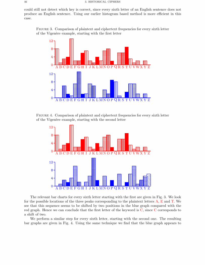
46 3. HISTORICAL CIPHERS
could still not detect which key is correct, since every sixth letter of an English sentence does notproduce an English sentence. Using our earlier histogram based method is more efficient in thiscase.
Figure 3. Comparison of plaintext and ciphertext frequencies for every sixth letterof the Vigenere example, starting with the first letter
0
4
8
12
A B C D E F G H I J K L MN O P Q R S T U VWX Y Z
0
4
8
12
A B C D E F G H I J K L MN O P Q R S T U VWX Y Z
Figure 4. Comparison of plaintext and ciphertext frequencies for every sixth letterof the Vigenere example, starting with the second letter
0
4
8
12
A B C D E F G H I J K L MN O P Q R S T U VWX Y Z
0
4
8
12
A B C D E F G H I J K L MN O P Q R S T U VWX Y����������������
Z
The relevant bar charts for every sixth letter starting with the first are given in Fig. 3. We lookfor the possible locations of the three peaks corresponding to the plaintext letters A, E and T. Wesee that this sequence seems to be shifted by two positions in the blue graph compared with thered graph. Hence we can conclude that the first letter of the keyword is C, since C corresponds toa shift of two.
We perform a similar step for every sixth letter, starting with the second one. The resultingbar graphs are given in Fig. 4. Using the same technique we find that the blue graph appears to
5. A PERMUTATION CIPHER 47
have been shifted along by 17 spaces, which corresponds to the second letter of the keyword beingequal to R.
Continuing in a similar way for the remaining four letters of the keyword we find the keywordis
CRYPTO.The underlying plaintext is then found to be:
Scrooge was better than his word. He did it all, and infinitely more; and to Tiny Tim, who didnot die, he was a second father. He became as good a friend, as good a master, and as good a man,as the good old city knew, or any other good old city, town, or borough, in the good old world.Some people laughed to see the alteration in him, but he let them laugh, and little heeded them;for he was wise enough to know that nothing ever happened on this globe, for good, at which somepeople did not have their fill of laughter in the outset; and knowing that such as these would beblind anyway, he thought it quite as well that they should wrinkle up their eyes in grins, as havethe malady in less attractive forms. His own heart laughed: and that was quite enough for him.
He had no further intercourse with Spirits, but lived upon the Total Abstinence Principle, everafterwards; and it was always said of him, that he knew how to keep Christmas well, if any manalive possessed the knowledge. May that be truly said of us, and all of us! And so, as Tiny Timobserved, God bless Us, Every One!
The above text is taken from A Christmas Carol by Charles Dickens.
5. A Permutation Cipher
The ideas behind substitution type ciphers forms part of the design of modern symmetricsystems. For example later we shall see that both DES and Rijndael make use of a componentcalled an S-Box, which is simply a substitution. The other component that is used in modernsymmetric ciphers is based on permutations.
Permutation ciphers have been around for a number of centuries. Here we shall describe thesimplest, which is particularly easy to break. We first fix a permutation group Sn and a permutation
σ ∈ Sn.
It is the value of σ which will be the secret key. As an example suppose we take
σ =(
1 2 3 4 52 4 1 3 5
)= (1243) ∈ S5.
Now take some plaintext, sayOnce upon a time there was a little girl called snow white.
We break the text into chunks of 5 lettersonceu ponat imeth erewa salit tlegi rlcal ledsn owwhi te.
We first pad the message, with some random letters, so that we have a multiple of five letters ineach chunk.
onceu ponat imeth erewa salit tlegi rlcal ledsn owwhi teahb.Then we take each five-letter chunk in turn and swap the letters around according to our secretpermutation σ. With our example we obtain
coenu npaot eitmh eewra lsiat etgli crall dlsdn wohwi atheb.We then remove the spaces, so as to hide the value of n, producing the ciphertext
coenunpaoteitmheewralsiatetglicralldlsdnwohwiatheb.However, breaking a permutation cipher is easy with a chosen plaintext attack, assuming the groupof permutations used (i.e. the value of n) is reasonably small. To attack this cipher we mount achosen plaintext attack, and ask one of the parties to encrypt the message
48 3. HISTORICAL CIPHERS
abcdefghijklmnopqrstuvwxyz,to obtain the ciphertext
cadbehfigjmknlorpsqtwuxvyz.We can then deduce that the permutation looks something like(
1 2 3 4 5 6 7 8 9 10 11 12 13 14 15 . . .2 4 1 3 5 7 9 6 8 10 12 14 11 13 15 . . .
).
We see that the sequence repeats (modulo 5) after every five steps and so the value of n is prob-ably equal to five. We can recover the key by simply taking the first five columns of the abovepermutation.
Chapter Summary
• Many early ciphers can be broken because they do not successfully hide the underlyingstatistics of the language.
• Important principles behind early ciphers are those of substitution and permutation.• Ciphers can either work on blocks of characters via some keyed algorithm or simply consist
of adding some keystream to each plaintext character.• Ciphers which aimed to get around these early problems often turned out to be weaker
than expected, either due to some design flaw or due to bad key management practicesadopted by operators.
Further Reading
The best book on the history of ciphers is that by Kahn. Kahn’s book is a weighty tome so thosewishing a more rapid introduction should consult the book by Singh. The book by Churchhousealso gives an overview of a number of historical ciphers.
R. Churchhouse. Codes and Ciphers. Julius Caesar, the Enigma and the Internet. CambridgeUniversity Press, 2001.
D. Kahn. The Codebreakers: The Comprehensive History of Secret Communication from AncientTimes to the Internet. Scribner, 1996.
S. Singh. The Codebook: The Evolution of Secrecy from Mary, Queen of Scots to Quantum Cryp-tography. Doubleday, 2000.
CHAPTER 4
The Enigma Machine
Chapter Goals
• To explain the working of the Enigma machine.• To explain how the Germans used the Enigma machine, in particular how session keys
were transmitted from the sender to the reciever.• To explain how this enabled Polish and later British cryptanalysts to read the German
traffic.• To explain the use of the Bombe in mounting known plaintext attacks.
1. Introduction
With the advent of the 1920s people saw the need for a mechanical encryption device. Takinga substitution cipher and then rotating it became seen as the ideal solution. This idea had actuallybeen used previously in a number of manual ciphers, but using machines it was seen how this couldbe done more efficiently. The rotors could be implemented using wires and then encryption couldbe done mechanically using an electrical circuit. By rotating the rotor we obtain a new substitutioncipher.
As an example, suppose the rotor used to produce the substitutions is given byABCDEFGHIJKLMNOPQRSTUVWXYZTMKGOYDSIPELUAVCRJWXZNHBQF
To encrypt the first letter we use the substitutions given byABCDEFGHIJKLMNOPQRSTUVWXYZTMKGOYDSIPELUAVCRJWXZNHBQF
However, to encrypt the second letter we rotate the rotor by one position and use the substitutionsABCDEFGHIJKLMNOPQRSTUVWXYZMKGOYDSIPELUAVCRJWXZNHBQFT
To encrypt the third letter we use the substitutionsABCDEFGHIJKLMNOPQRSTUVWXYZKGOYDSIPELUAVCRJWXZNHBQFTM
and so on. This gives us a polyalphabetic substitution cipher with 26 alphabets.The most famous of these machines was the Enigma machine used by the Germans in World
War II. We shall describe the most simple version of Enigma which only used three such rotors,chosen from the following set of five.
ABCDEFGHIJKLMNOPQRSTUVWXYZEKMFLGDQVZNTOWYHXUSPAIBRCJAJDKSIRUXBLHWTMCQGZNPYFVOEBDFHJLCPRTXVZNYEIWGAKMUSQOESOVPZJAYQUIRHXLNFTGKDCMWB
49
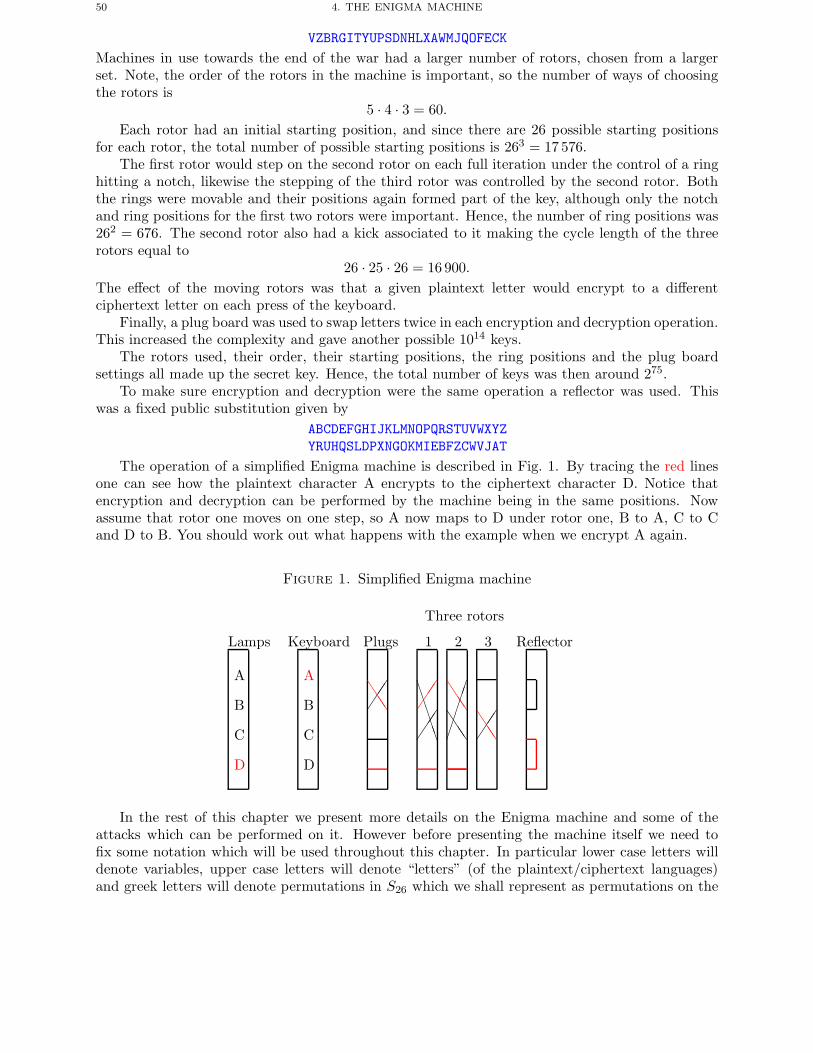
50 4. THE ENIGMA MACHINE
VZBRGITYUPSDNHLXAWMJQOFECK
Machines in use towards the end of the war had a larger number of rotors, chosen from a largerset. Note, the order of the rotors in the machine is important, so the number of ways of choosingthe rotors is
5 · 4 · 3 = 60.Each rotor had an initial starting position, and since there are 26 possible starting positions
for each rotor, the total number of possible starting positions is 263 = 17576.The first rotor would step on the second rotor on each full iteration under the control of a ring
hitting a notch, likewise the stepping of the third rotor was controlled by the second rotor. Boththe rings were movable and their positions again formed part of the key, although only the notchand ring positions for the first two rotors were important. Hence, the number of ring positions was262 = 676. The second rotor also had a kick associated to it making the cycle length of the threerotors equal to
26 · 25 · 26 = 16 900.The effect of the moving rotors was that a given plaintext letter would encrypt to a differentciphertext letter on each press of the keyboard.
Finally, a plug board was used to swap letters twice in each encryption and decryption operation.This increased the complexity and gave another possible 1014 keys.
The rotors used, their order, their starting positions, the ring positions and the plug boardsettings all made up the secret key. Hence, the total number of keys was then around 275.
To make sure encryption and decryption were the same operation a reflector was used. Thiswas a fixed public substitution given by
ABCDEFGHIJKLMNOPQRSTUVWXYZYRUHQSLDPXNGOKMIEBFZCWVJAT
The operation of a simplified Enigma machine is described in Fig. 1. By tracing the red linesone can see how the plaintext character A encrypts to the ciphertext character D. Notice thatencryption and decryption can be performed by the machine being in the same positions. Nowassume that rotor one moves on one step, so A now maps to D under rotor one, B to A, C to Cand D to B. You should work out what happens with the example when we encrypt A again.
Figure 1. Simplified Enigma machine
Lamps
A
B
C
D
Keyboard
A
B
C
D
Plugs
������
Three rotors
1
�����
���
���
2
���
��������
3
������
Reflector
In the rest of this chapter we present more details on the Enigma machine and some of theattacks which can be performed on it. However before presenting the machine itself we need tofix some notation which will be used throughout this chapter. In particular lower case letters willdenote variables, upper case letters will denote “letters” (of the plaintext/ciphertext languages)and greek letters will denote permutations in S26 which we shall represent as permutations on the
2. AN EQUATION FOR THE ENIGMA 51
upper case letters. Hence x can equal X and Y , but X can only ever represent X, whereas χ couldrepresent (XY ) or (ABC).
Permutations will usually be given in cycle notation. One always has to make a choice as towhether we multiply permutations from left to right, or right to left. We decide to use the left toright method, hence
(ABCD)(BE)(CD) = (AEBD).Permutations hence act on the right of letters, something we will denote by xσ, e.g.
A(ABCD)(XY ) = B.
This is consistent with the usual notation of right action for groups acting on sets. See AppendixA for more details about permutations.
We now collect some basic facts and theorems about permutations which we will need in thesequel.
Theorem 4.1. Two permutations σ and τ which are conjugate, i.e. for which σ = λ · τ · λ−1
for some permutation λ, have the same cycle structure.
We define the support of a permutation to be the set of letters which are not fixed by thepermutation. Hence, if σ acts on the set of letters L, then as usual we denote by Lσ the set of fixedpoints and hence the support is given by
L \ Lσ.Theorem 4.2. If two permutations, with the same support, consist only of disjoint transposi-
tions then their product contains an even number of disjoint cycles of the same lengths.If a permutation with support an even number of symbols has an even number of disjoint cycles
of the same lengths, then the permutation can be written as a product of two permutations each ofwhich consists of disjoint transpositions.
In many places we need an algorithm to solve the following problem: Given αi, βi ∈ S26, fori = 1, . . . ,m find γ ∈ S26 such that
αi = γ−1 · βi · γ for i = 1 . . . ,m.
Note, there could be many such solutions γ, but in the situations we will apply it we expect thereto be only a few.
For example suppose we have one such equation with
α1 = (AFCNE)(BWXHUJOG)(DV IQZ)(KLMY TRPS),β1 = (AEY SXWUJ)(BFZNO)(CDPKQ)(GHIV LMRT )
We need to determine the structure of the permutation γ such that
α1 = γ−1 · β1 · γ.We first look at what should A map to under γ. If Aγ = B, then from α1 and β1 we must haveEγ = W , which in turn implies Y γ = X. Carrying on in this way via a pruned depth first searchwe can determine a set of possible values for γ. Such an algorithm is relatively simple to writedown in C, using a recursive procedure call. It however of course been a bit of a pain to do this byhand, as one would need to in the 1930’s and 1940’s.
2. An Equation For The Enigma
To aid our discussion in later sections we now describe the Enigma machine as a permutationequation. We first assume a canonical map between letters and the integers {0, 1, . . . , 25} such that0 ← A, 1 ← B, etc and we assume a standard three wheel Enigma machine.
The wheel which turns the fastest we shall call rotor one, whilst the one which turns the slowestwe shall call rotor three. This means that when looking at a real machine rotor three is the left
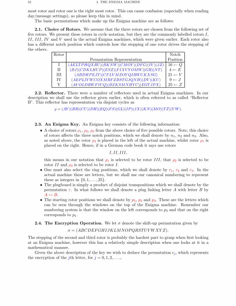
52 4. THE ENIGMA MACHINE
most rotor and rotor one is the right most rotor. This can cause confusion (especially when readingday/message settings), so please keep this in mind.
The basic permutations which make up the Enigma machine are as follows:
2.1. Choice of Rotors. We assume that the three rotors are chosen from the following set offive rotors. We present these rotors in cycle notation, but they are the commonly labelled rotors I,II, III, IV and V used in the actual Enigma machines, which were given earlier. Each rotor alsohas a different notch position which controls how the stepping of one rotor drives the stepping ofthe others.
Rotor NotchPermutation Representation Position
I (AELTPHQXRU)(BKNW )(CMOY )(DFG)(IV )(JZ) 16 ← QII (BJ)(CDKLHUP )(ESZ)(FIXV Y OMW )(GR)(NT ) 4 ← EIII (ABDHPEJT )(CFLVMZOY QIRWUKXSG) 21 ← VIV (AEPLIYWCOXMRFZBSTGJQNH)(DV )(KU) 9 ← JV (AV OLDRWFIUQ)(BZKSMNHYC)(EGTJPX) 25 ← Z
2.2. Reflector. There were a number of reflectors used in actual Enigma machines. In ourdescription we shall use the reflector given earlier, which is often referred to as called “ReflectorB”. This reflector has representation via disjoint cycles as
= (AY )(BR)(CU)(DH)(EQ)(FS)(GL)(IP )(JX)(KN)(MO)(TZ)(V W ).
2.3. An Enigma Key. An Enigma key consists of the following information:• A choice of rotors ρ1, ρ2, ρ3 from the above choice of five possible rotors. Note, this choice
of rotors affects the three notch positions, which we shall denote by n1, n2 and n3. Also,as noted above, the rotor ρ3 is placed in the left of the actual machine, whilst rotor ρ1 isplaced on the right. Hence, if in a German code book it says use rotors
I, II, III,
this means in our notation that ρ1 is selected to be rotor III, that ρ2 is selected to berotor II and ρ3 is selected to be rotor I.
• One must also select the ring positions, which we shall denote by r1, r2 and r3. In theactual machine these are letters, but we shall use our canonical numbering to representthese as integers in {0, 1, . . . , 25}.
• The plugboard is simply a product of disjoint transpositions which we shall denote by thepermutation τ . In what follows we shall denote a plug linking letter A with letter B byA↔ B.
• The starting rotor positions we shall denote by p1, p2 and p3. These are the letters whichcan be seen through the windows on the top of the Enigma machine. Remember ournumbering system is that the window on the left corresponds to p3 and that on the rightcorresponds to p1.
2.4. The Encryption Operation. We let σ denote the shift-up permutation given by
σ = (ABCDEFGHIJKLMNOPQRSTUVWXY Z).
The stepping of the second and third rotor is probably the hardest part to grasp when first lookingat an Enigma machine, however this has a relatively simple description when one looks at it in amathematical manner.
Given the above description of the key we wish to deduce the permutation εj , which representsthe encryption of the jth letter, for j = 0, 1, 2, . . . ,.
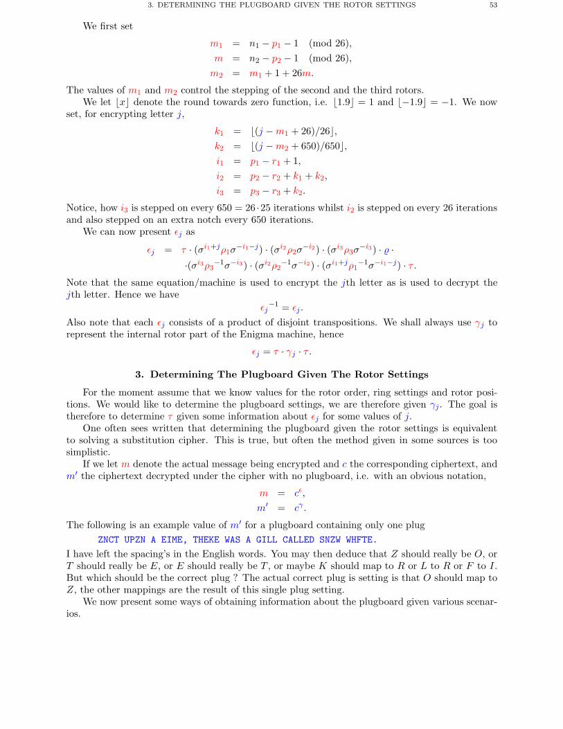
3. DETERMINING THE PLUGBOARD GIVEN THE ROTOR SETTINGS 53
We first set
m1 = n1 − p1 − 1 (mod 26),m = n2 − p2 − 1 (mod 26),m2 = m1 + 1 + 26m.
The values of m1 and m2 control the stepping of the second and the third rotors.We let �x� denote the round towards zero function, i.e. �1.9� = 1 and �−1.9� = −1. We now
set, for encrypting letter j,
k1 = �(j −m1 + 26)/26�,k2 = �(j −m2 + 650)/650�,i1 = p1 − r1 + 1,i2 = p2 − r2 + k1 + k2,
i3 = p3 − r3 + k2.
Notice, how i3 is stepped on every 650 = 26 ·25 iterations whilst i2 is stepped on every 26 iterationsand also stepped on an extra notch every 650 iterations.
We can now present εj as
εj = τ · (σi1+jρ1σ−i1−j) · (σi2ρ2σ
−i2) · (σi3ρ3σ−i3) · ·
·(σi3ρ3−1σ−i3) · (σi2ρ2
−1σ−i2) · (σi1+jρ1−1σ−i1−j) · τ .
Note that the same equation/machine is used to encrypt the jth letter as is used to decrypt thejth letter. Hence we have
εj−1 = εj .
Also note that each εj consists of a product of disjoint transpositions. We shall always use γj torepresent the internal rotor part of the Enigma machine, hence
εj = τ · γj · τ .
3. Determining The Plugboard Given The Rotor Settings
For the moment assume that we know values for the rotor order, ring settings and rotor posi-tions. We would like to determine the plugboard settings, we are therefore given γj . The goal istherefore to determine τ given some information about εj for some values of j.
One often sees written that determining the plugboard given the rotor settings is equivalentto solving a substitution cipher. This is true, but often the method given in some sources is toosimplistic.
If we let m denote the actual message being encrypted and c the corresponding ciphertext, andm′ the ciphertext decrypted under the cipher with no plugboard, i.e. with an obvious notation,
m = cε,
m′ = cγ .
The following is an example value of m′ for a plugboard containing only one plugZNCT UPZN A EIME, THEKE WAS A GILL CALLED SNZW WHFTE.
I have left the spacing’s in the English words. You may then deduce that Z should really be O, orT should really be E, or E should really be T , or maybe K should map to R or L to R or F to I.But which should be the correct plug ? The actual correct plug is setting is that O should map toZ, the other mappings are the result of this single plug setting.
We now present some ways of obtaining information about the plugboard given various scenar-ios.
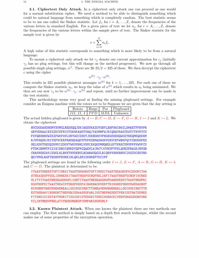
54 4. THE ENIGMA MACHINE
3.1. Ciphertext Only Attack. In a ciphertext only attack one can proceed as one wouldfor a normal substitution cipher. We need a method to be able to distinguish something whichcould be natural language from something which is completely random. The best statistic seemsto be to use one called the Sinkov statistic. Let fi, for i = A, . . . , Z, denote the frequencies of thevarious letters in standard English. For a given piece of text we let ni, for i = A, . . . , Z, denotethe frequencies of the various letters within the sample piece of text. The Sinkov statistic for thesample text is given by
s =Z∑i=A
nifi.
A high value of this statistic corresponds to something which is more likely to be from a naturallanguage.
To mount a ciphertext only attack we let γj denote our current approximation for εj (initiallyγj has no plug settings, but this will change as the method progresses). We now go through allpossible single plug settings, α(). There are 26·25/2 = 325 of these. We then decrypt the ciphertextc using the cipher
α(k) · γj · α(k).
This results in 325 possible plaintext messages m(k) for k = 1, . . . , 325. For each one of these wecompute the Sinkov statistic sk, we keep the value of α(k) which results in sk being minimized. Wethen set our new γj to be α(k) · γj · α(k) and repeat, until no further improvement can be made inthe test statistic.
This methodology seems very good at finding the missing plugboard settings. For exampleconsider an Enigma machine with the rotors set to be Suppose we are given that the day setting is
Rotors Rings Pos PlugboardIII, II, I PPD MDL Unknown
The actual hidden plugboard is given by A↔ B, C ↔ D, E ↔ F , G↔ H, I ↔ J and K ↔ L. Weobtain the ciphertext
HUCDODANDHOMYXUMGLREDSQQJDNJAEXUKAZOYGBYLEWFNWIBWILSMAETFFBVPRGBYUDNAAIEVZZKCUFNIUTOKNKAWUTUWQJYAUHMFWJNIQHAYNAGTDGTCTNYKTCUFGYQBSRRUWZKZFWKPGVLUHYWZCZSOYJNXHOSKVPHGSGSXEOQWOZYBXQMKQDDXMBJUPSQODJNIYEPUCEXFRHDQDAQDTFKPSZEMASWGKVOXUCEYWBKFQCYZBOGSFESOELKDUTDEUQZKMUIZOGVTWKUVBHLVXMIXKQGUMMQHDLKFTKRXCUNUPPFKWUFCUPTDMJBMMTPIZIXINRUIEMKDYQFMIQAEVLWJRCYJCUKUFYPSLQUEZFBAGSJHVOBCHAKHGHZAVJZWOLWLBKNTHVDEBULROARWOQGZLRIQBVVSNKRNUCIKSZUCXEYBDQKCVMGLRGFTBGHUPDUHXIHLQKLEMIZKHDEPTDCIPF
The plugboard settings are found in the following order I ↔ J , E ↔ F , A↔ B, G↔ H, K ↔ Land C ↔ D. The plaintext is determined to be.
ITWASTHEBESTOFTIMESITWASTHEWORSTOFTIMESITWASTHEAGEOFWISDOMITWASTHEAGEOFFOOLISHNESSITWASTHEEPOCHOFBELIEFITWASTHEEPOCHOFINCREDULITYITWASTHESEASONOFLIGHTITWASTHESEASONOFDARKNESSITWASTHESPRINGOFHOPEITWASTHEWINTEROFDESPAIRWEHADEVERYTHINGBEFOREUSWEHADNOTHINGBEFOREUSWEWEREALLGOINGDIRECTTOHEAVENWEWEREALLGOINGDIRECTTHEOTHERWAYINSHORTTHEPERIODWASSOFARLIKETHEPRESENTPERIODTHATSOMEOFITSNOISIESTAUTHORITIESINSISTEDONITSBEINGRECEIVEDFORGOODORFOREVILINTHESUPERLATIVEDEGREEOFCOMPARISONONLY
3.2. Known Plaintext Attack. When one knows the plaintext there are two methods onecan employ. The first method is simply based on a depth first search technique, whilst the secondmakes use of some properties of the encryption operation.
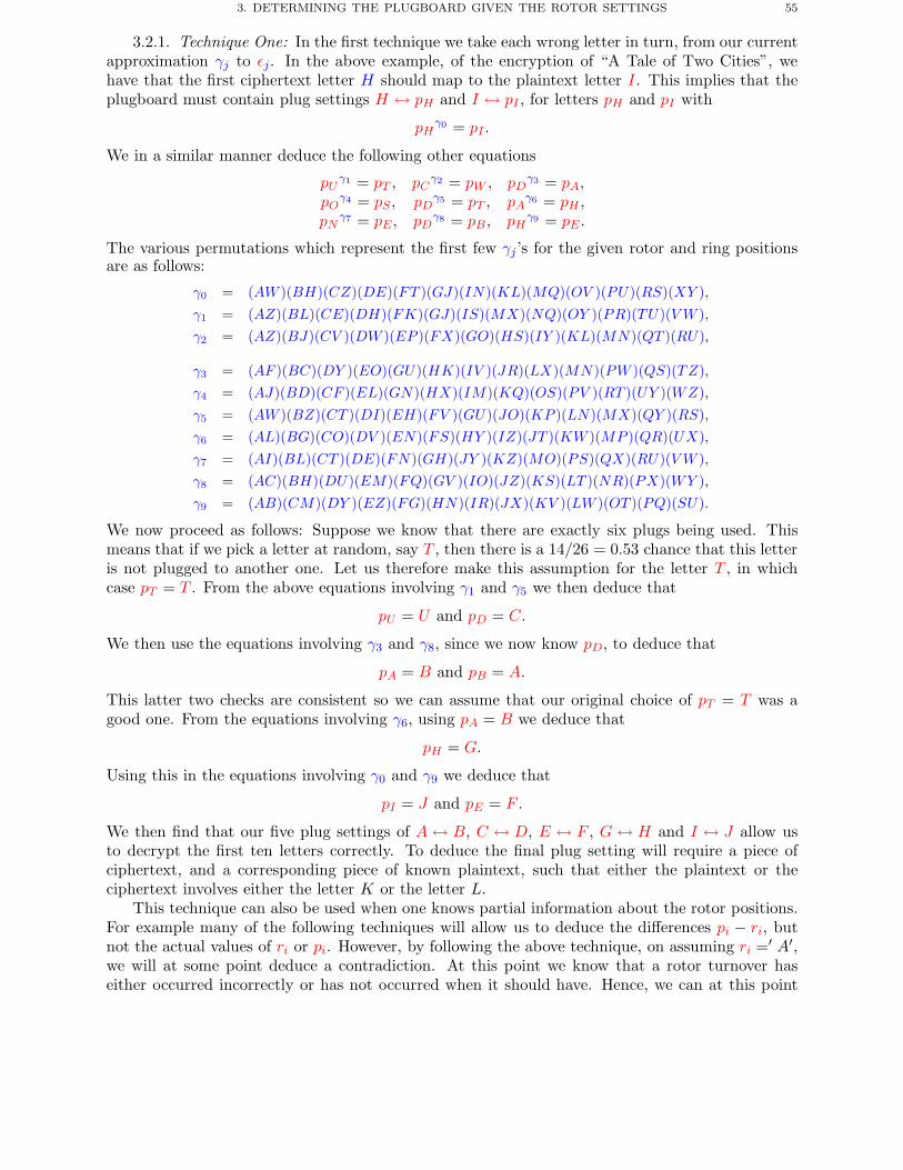
3. DETERMINING THE PLUGBOARD GIVEN THE ROTOR SETTINGS 55
3.2.1. Technique One: In the first technique we take each wrong letter in turn, from our currentapproximation γj to εj. In the above example, of the encryption of “A Tale of Two Cities”, wehave that the first ciphertext letter H should map to the plaintext letter I. This implies that theplugboard must contain plug settings H ↔ pH and I ↔ pI , for letters pH and pI with
pHγ0 = pI .
We in a similar manner deduce the following other equations
pUγ1 = pT , pC
γ2 = pW , pDγ3 = pA,
pOγ4 = pS, pD
γ5 = pT , pAγ6 = pH ,
pNγ7 = pE, pD
γ8 = pB , pHγ9 = pE.
The various permutations which represent the first few γj’s for the given rotor and ring positionsare as follows:
γ0 = (AW )(BH)(CZ)(DE)(FT )(GJ)(IN)(KL)(MQ)(OV )(PU)(RS)(XY ),γ1 = (AZ)(BL)(CE)(DH)(FK)(GJ)(IS)(MX)(NQ)(OY )(PR)(TU)(VW ),γ2 = (AZ)(BJ)(CV )(DW )(EP )(FX)(GO)(HS)(IY )(KL)(MN)(QT )(RU),
γ3 = (AF )(BC)(DY )(EO)(GU)(HK)(IV )(JR)(LX)(MN)(PW )(QS)(TZ),γ4 = (AJ)(BD)(CF )(EL)(GN)(HX)(IM)(KQ)(OS)(PV )(RT )(UY )(WZ),γ5 = (AW )(BZ)(CT )(DI)(EH)(FV )(GU)(JO)(KP )(LN)(MX)(QY )(RS),γ6 = (AL)(BG)(CO)(DV )(EN)(FS)(HY )(IZ)(JT )(KW )(MP )(QR)(UX),γ7 = (AI)(BL)(CT )(DE)(FN)(GH)(JY )(KZ)(MO)(PS)(QX)(RU)(VW ),γ8 = (AC)(BH)(DU)(EM)(FQ)(GV )(IO)(JZ)(KS)(LT )(NR)(PX)(WY ),γ9 = (AB)(CM)(DY )(EZ)(FG)(HN)(IR)(JX)(KV )(LW )(OT )(PQ)(SU).
We now proceed as follows: Suppose we know that there are exactly six plugs being used. Thismeans that if we pick a letter at random, say T , then there is a 14/26 = 0.53 chance that this letteris not plugged to another one. Let us therefore make this assumption for the letter T , in whichcase pT = T . From the above equations involving γ1 and γ5 we then deduce that
pU = U and pD = C.
We then use the equations involving γ3 and γ8, since we now know pD, to deduce that
pA = B and pB = A.
This latter two checks are consistent so we can assume that our original choice of pT = T was agood one. From the equations involving γ6, using pA = B we deduce that
pH = G.
Using this in the equations involving γ0 and γ9 we deduce that
pI = J and pE = F.
We then find that our five plug settings of A↔ B, C ↔ D, E ↔ F , G↔ H and I ↔ J allow usto decrypt the first ten letters correctly. To deduce the final plug setting will require a piece ofciphertext, and a corresponding piece of known plaintext, such that either the plaintext or theciphertext involves either the letter K or the letter L.
This technique can also be used when one knows partial information about the rotor positions.For example many of the following techniques will allow us to deduce the differences pi − ri, butnot the actual values of ri or pi. However, by following the above technique, on assuming ri =′ A′,we will at some point deduce a contradiction. At this point we know that a rotor turnover haseither occurred incorrectly or has not occurred when it should have. Hence, we can at this point
56 4. THE ENIGMA MACHINE
backtrack and deduce the correct turnover. For an example of this technique at work see the lattersection on the Bombe.
3.2.2. Technique Two: A second method is possible when less than 13 plugs used. In theplaintext obtained under γj a number of incorrect letters will appear. Again we let m denote theactual plaintext and m′ the plaintext derived with the current (possibly empty) plugboard setting.We suppose there are t plugs left to find.
Suppose we concentrate on each places for which the incorrect plaintext letter A occurs, i.e. alloccurances of A in the plaintext m which are wrong. Let x denote the corresponding ciphertextletter, there are two possible cases which can occur
• The letter x should be plugged to an unknown letter. In which case the resulting letter inthe message m′ will behave randomly (assuming γj is acts like a random permutation).
• The letter x does not occur in a plugboard setting. In which case the resulting incorrectplaintext character is the one which should be plugged to A in the actual cipher.
Assuming ciphertext letters are uniformly distributed, the first occurance will occur with probabilityt/13, whilst the alternative will occur with probability 1 − t/13. This gives the following methodto determine which letter A should be connected to. For all letters A in the plaintext m computethe frequency of the corresponding letter in the approximate plaintext m′. The letter which hasthe highest frequency is highly likely to be the one which should be connect to A on the plugboard.Indeed we expect this letter to occur for a proportion of the letters given by 1 − t/13, all otherletters we expect to occur with a proportion of t/(13 · 26) each.
The one problem with this second technique is that it requires a relatively large amount ofknown plaintext. Hence, in practice the first technique is more likely to be used.
3.3. Knowledge of εj for some j’s. If we know the value of the permutation εj for valuesof j ∈ S, then we have the following equation
εj = τ · γj · τ for j ∈ S.Since τ = τ−1 this allows us to compute possible values of τ using our previous method for solvingthis conjugation problem. This might not determine the whole plugboard but it will determineenough for other methods to be used.
3.4. Knowledge of εj · εj+3 for some j’s. A similar method to the previous one applies inthis case, as if we know εj · εj+3 for all j ∈ S and we know γj , then we have the equation
(εj · εj+3) = τ · (γj · γj+3) · τ for j ∈ S.
4. Double Encryption Of Message Keys
The polish mathematicians Jerzy Rozycki, Henryk Zygalski and Marian Rejewski were thefirst to find ways of analysing the Enigma machine. To understand their methods one must firstunderstand how the Germans used the machine. On each day the machine was set up with a key,as above, which was chosen by looking up in a code book. Each subnet would have a different daykey.
To encipher a message the sending operator decided on a message key. The message key wouldbe a sequence of three letters, say DHI. The message key needs to be transported to the recipient.Using the day key, the message key would be enciphered twice. The double enciphering is to act asa form of error control. Hence, DHI might be enciphered as XHJKLM . Note, that D encryptsto X and then K, this is a property of the Enigma machine.
The receiver would obtain XHJKLM and then decrypt this to obtain DHI. Both operatorswould then move the wheels around to the positions D, H and I, i.e. they would turn the wheelsso that D was in the leftmost window, H in the middle one and I in the rightmost window. Thenthe actual message would be enciphered.
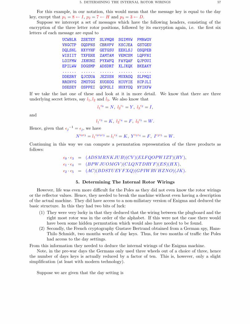
5. DETERMINING THE INTERNAL ROTOR WIRINGS 57
For this example, in our notation, this would mean that the message key is equal to the daykey, except that p1 = 8 ← I, p2 = 7 ← H and p3 = 3 ← D.
Suppose we intercept a set of messages which have the following headers, consisting of theencryption of the three letter rotor positions, followed by its encryption again, i.e. the first sixletters of each message are equal to
UCWBLR ZSETEY SLVMQH SGIMVW PMRWGVVNGCTP OQDPNS CBRVPV KSCJEA GSTGEUDQLSNL HXYYHF GETGSU EEKLSJ OSQPEBWISIIT TXFEHX ZAMTAM VEMCSM LQPFNILOIFMW JXHUHZ PYXWFQ FAYQAF QJPOUIEPILWW DOGSMP ADSDRT XLJXQK BKEAKY...... ...... ...... ...... ......DDESRY QJCOUA JEZUSN MUXROQ SLPMQIRRONYG ZMOTGG XUOXOG HIUYIE KCPJLIDSESEY OSPPEI QCPOLI HUXYOQ NYIKFW
If we take the last one of these and look at it in more detail. We know that there are threeunderlying secret letters, say l1, l2 and l3. We also know that
l1ε0 = N, l2
ε1 = Y , l3ε2 = I,
andl1ε3 = K, l2
ε4 = F, l3ε5 = W.
Hence, given that εj−1 = εj, we have
N ε0ε3 = l1ε0ε0ε3 = l1
ε3 = K, Y ε1ε4 = F, Iε2ε5 = W.
Continuing in this way we can compute a permutation representation of the three products asfollows:
ε0 · ε3 = (ADSMRNKJUB)(CV )(ELFQOPWIZT )(HY ),ε1 · ε4 = (BPWJUOMGV )(CLQNTDRY F )(ES)(HX),ε2 · ε5 = (AC)(BDSTUEY FXQ)(GPIWRV HZNO)(JK).
5. Determining The Internal Rotor Wirings
However, life was even more difficult for the Poles as they did not even know the rotor wiringsor the reflector values. Hence, they needed to break the machine without even having a descriptionof the actual machine. They did have access to a non-miliatary version of Enigma and deduced thebasic structure. In this they had two bits of luck:
(1) They were very lucky in that they deduced that the wiring between the plugboard and theright most rotor was in the order of the alphabet. If this were not the case there wouldhave been some hidden permutation which would also have needed to be found.
(2) Secondly, the French cryptography Gustave Bertrand obtained from a German spy, Hans-Thilo Schmidt, two months worth of day keys. Thus, for two months of traffic the Poleshad access to the day settings.
From this information they needed to deduce the internal wirings of the Enigma machine.Note, in the pre-war days the Germans only used three wheels out of a choice of three, hence
the number of days keys is actually reduced by a factor of ten. This is, however, only a slightsimplification (at least with modern technology).
Suppose we are given that the day setting is
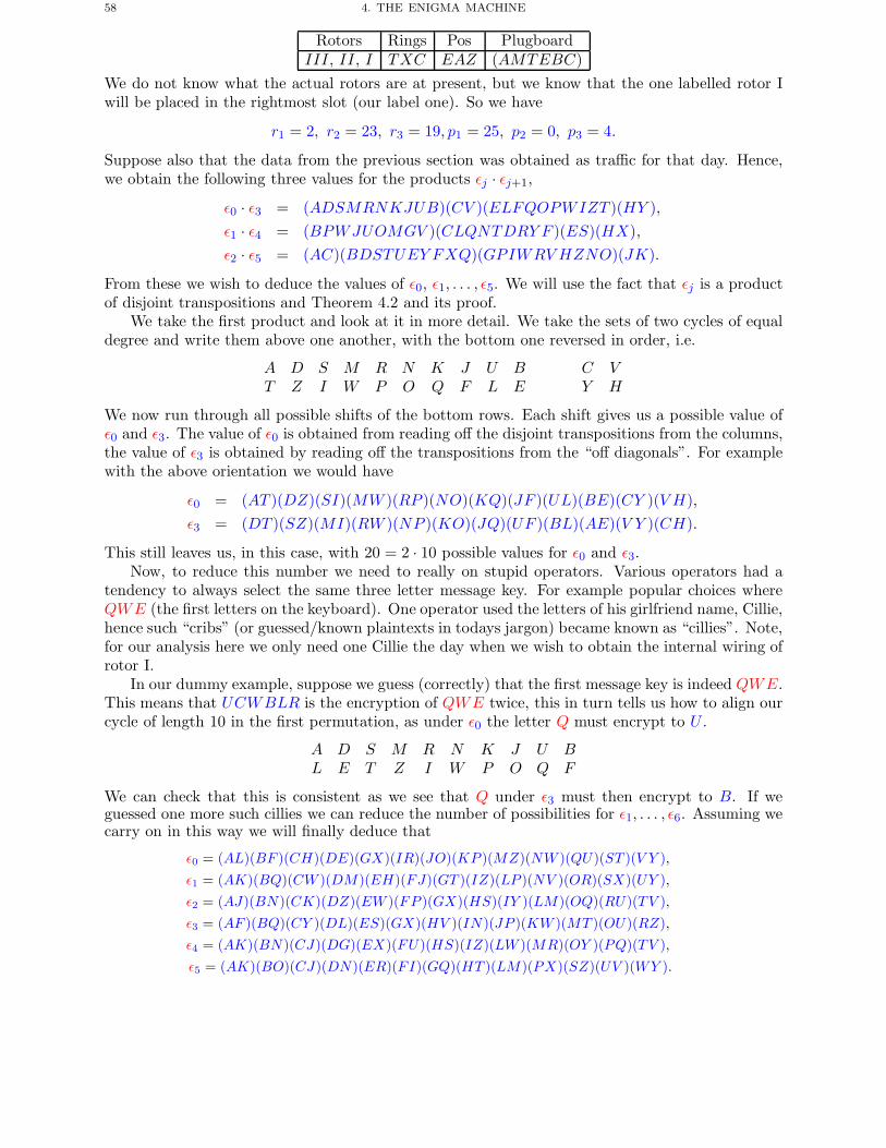
58 4. THE ENIGMA MACHINE
Rotors Rings Pos PlugboardIII, II, I TXC EAZ (AMTEBC)
We do not know what the actual rotors are at present, but we know that the one labelled rotor Iwill be placed in the rightmost slot (our label one). So we have
r1 = 2, r2 = 23, r3 = 19, p1 = 25, p2 = 0, p3 = 4.
Suppose also that the data from the previous section was obtained as traffic for that day. Hence,we obtain the following three values for the products εj · εj+1,
ε0 · ε3 = (ADSMRNKJUB)(CV )(ELFQOPWIZT )(HY ),ε1 · ε4 = (BPWJUOMGV )(CLQNTDRY F )(ES)(HX),ε2 · ε5 = (AC)(BDSTUEY FXQ)(GPIWRV HZNO)(JK).
From these we wish to deduce the values of ε0, ε1, . . . , ε5. We will use the fact that εj is a productof disjoint transpositions and Theorem 4.2 and its proof.
We take the first product and look at it in more detail. We take the sets of two cycles of equaldegree and write them above one another, with the bottom one reversed in order, i.e.
A D S M R N K J U BT Z I W P O Q F L E
C VY H
We now run through all possible shifts of the bottom rows. Each shift gives us a possible value ofε0 and ε3. The value of ε0 is obtained from reading off the disjoint transpositions from the columns,the value of ε3 is obtained by reading off the transpositions from the “off diagonals”. For examplewith the above orientation we would have
ε0 = (AT )(DZ)(SI)(MW )(RP )(NO)(KQ)(JF )(UL)(BE)(CY )(V H),ε3 = (DT )(SZ)(MI)(RW )(NP )(KO)(JQ)(UF )(BL)(AE)(V Y )(CH).
This still leaves us, in this case, with 20 = 2 · 10 possible values for ε0 and ε3.Now, to reduce this number we need to really on stupid operators. Various operators had a
tendency to always select the same three letter message key. For example popular choices whereQWE (the first letters on the keyboard). One operator used the letters of his girlfriend name, Cillie,hence such “cribs” (or guessed/known plaintexts in todays jargon) became known as “cillies”. Note,for our analysis here we only need one Cillie the day when we wish to obtain the internal wiring ofrotor I.
In our dummy example, suppose we guess (correctly) that the first message key is indeed QWE.This means that UCWBLR is the encryption of QWE twice, this in turn tells us how to align ourcycle of length 10 in the first permutation, as under ε0 the letter Q must encrypt to U .
A D S M R N K J U BL E T Z I W P O Q F
We can check that this is consistent as we see that Q under ε3 must then encrypt to B. If weguessed one more such cillies we can reduce the number of possibilities for ε1, . . . , ε6. Assuming wecarry on in this way we will finally deduce that
ε0 = (AL)(BF )(CH)(DE)(GX)(IR)(JO)(KP )(MZ)(NW )(QU)(ST )(V Y ),ε1 = (AK)(BQ)(CW )(DM)(EH)(FJ)(GT )(IZ)(LP )(NV )(OR)(SX)(UY ),ε2 = (AJ)(BN)(CK)(DZ)(EW )(FP )(GX)(HS)(IY )(LM)(OQ)(RU)(TV ),ε3 = (AF )(BQ)(CY )(DL)(ES)(GX)(HV )(IN)(JP )(KW )(MT )(OU)(RZ),ε4 = (AK)(BN)(CJ)(DG)(EX)(FU)(HS)(IZ)(LW )(MR)(OY )(PQ)(TV ),ε5 = (AK)(BO)(CJ)(DN)(ER)(FI)(GQ)(HT )(LM)(PX)(SZ)(UV )(WY ).
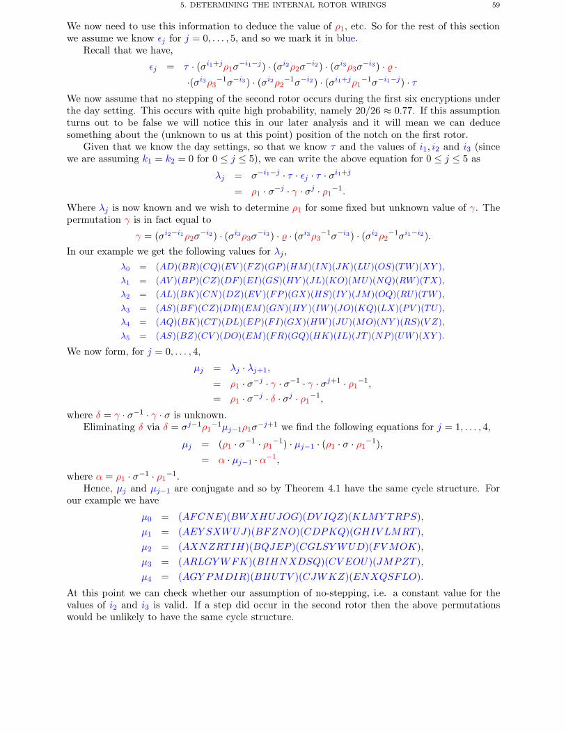
5. DETERMINING THE INTERNAL ROTOR WIRINGS 59
We now need to use this information to deduce the value of ρ1, etc. So for the rest of this sectionwe assume we know εj for j = 0, . . . , 5, and so we mark it in blue.
Recall that we have,
εj = τ · (σi1+jρ1σ−i1−j) · (σi2ρ2σ
−i2) · (σi3ρ3σ−i3) · ·
·(σi3ρ3−1σ−i3) · (σi2ρ2
−1σ−i2) · (σi1+jρ1−1σ−i1−j) · τ
We now assume that no stepping of the second rotor occurs during the first six encryptions underthe day setting. This occurs with quite high probability, namely 20/26 ≈ 0.77. If this assumptionturns out to be false we will notice this in our later analysis and it will mean we can deducesomething about the (unknown to us at this point) position of the notch on the first rotor.
Given that we know the day settings, so that we know τ and the values of i1, i2 and i3 (sincewe are assuming k1 = k2 = 0 for 0 ≤ j ≤ 5), we can write the above equation for 0 ≤ j ≤ 5 as
λj = σ−i1−j · τ · εj · τ · σi1+j= ρ1 · σ−j · γ · σj · ρ1
−1.
Where λj is now known and we wish to determine ρ1 for some fixed but unknown value of γ. Thepermutation γ is in fact equal to
γ = (σi2−i1ρ2σ−i2) · (σi3ρ3σ
−i3) · · (σi3ρ3−1σ−i3) · (σi2ρ2
−1σi1−i2).In our example we get the following values for λj ,
λ0 = (AD)(BR)(CQ)(EV )(FZ)(GP )(HM)(IN)(JK)(LU)(OS)(TW )(XY ),λ1 = (AV )(BP )(CZ)(DF )(EI)(GS)(HY )(JL)(KO)(MU)(NQ)(RW )(TX),λ2 = (AL)(BK)(CN)(DZ)(EV )(FP )(GX)(HS)(IY )(JM)(OQ)(RU)(TW ),λ3 = (AS)(BF )(CZ)(DR)(EM)(GN)(HY )(IW )(JO)(KQ)(LX)(PV )(TU),λ4 = (AQ)(BK)(CT )(DL)(EP )(FI)(GX)(HW )(JU)(MO)(NY )(RS)(V Z),λ5 = (AS)(BZ)(CV )(DO)(EM)(FR)(GQ)(HK)(IL)(JT )(NP )(UW )(XY ).
We now form, for j = 0, . . . , 4,
μj = λj · λj+1,
= ρ1 · σ−j · γ · σ−1 · γ · σj+1 · ρ1−1,
= ρ1 · σ−j · δ · σj · ρ1−1,
where δ = γ · σ−1 · γ · σ is unknown.Eliminating δ via δ = σj−1ρ1
−1μj−1ρ1σ−j+1 we find the following equations for j = 1, . . . , 4,
μj = (ρ1 · σ−1 · ρ1−1) · μj−1 · (ρ1 · σ · ρ1
−1),
= α · μj−1 · α−1,
where α = ρ1 · σ−1 · ρ1−1.
Hence, μj and μj−1 are conjugate and so by Theorem 4.1 have the same cycle structure. Forour example we have
μ0 = (AFCNE)(BWXHUJOG)(DV IQZ)(KLMY TRPS),μ1 = (AEY SXWUJ)(BFZNO)(CDPKQ)(GHIV LMRT ),μ2 = (AXNZRTIH)(BQJEP )(CGLSYWUD)(FVMOK),μ3 = (ARLGYWFK)(BIHNXDSQ)(CV EOU)(JMPZT ),μ4 = (AGY PMDIR)(BHUTV )(CJWKZ)(ENXQSFLO).
At this point we can check whether our assumption of no-stepping, i.e. a constant value for thevalues of i2 and i3 is valid. If a step did occur in the second rotor then the above permutationswould be unlikely to have the same cycle structure.
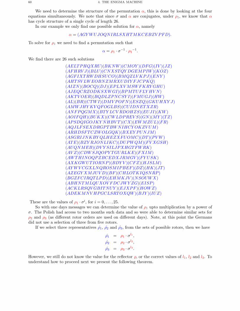
60 4. THE ENIGMA MACHINE
We need to determine the structure of the permutation α, this is done by looking at the fourequations simultaneously. We note that since σ and α are conjugates, under ρ1, we know that αhas cycle structure of a single cycle of length 26.
In our example we only find one possible solution for α, namely
α = (AGYWUJOQNIRLSXHTMKCEBZV PFD).
To solve for ρ1 we need to find a permutation such that
α = ρ1 · σ−1 · ρ1−1.
We find there are 26 such solutions
(AELTPHQXRU)(BKNW )(CMOY )(DFG)(IV )(JZ)(AFHRV J)(BLU)(CNXSTQY DGEMPIW )(KOZ)(AGFIXTRWDHSUCO)(BMQZLVKPJ)(ENY )(AHTSV LWEOBNZMRXUDIY FJCPKQ)(AIZN)(BOCQ)(DJ)(EPLXVMSWFKRYGHU)(AJEQCRZODKSXWGI)(BPMTUFLYHV N)(AKTV OER)(BQDLZPNCSY I)(FMUGJ)(HW )(AL)(BR)(CTWI)(DMV POFN)(ESZQ)(GKUHXY J)(AMWJHYKVQFOGLBS)(CUIDNETXZR)(ANFPQGMX)(BTY LCV RDOHZS)(EUJI)(KW )(AOIFQH)(BUKX)(CWLDPREV S)(GN)(MY )(TZ)(APSDQIGOJKY NHBV T )(CX)(EWMZUL)(FR)(AQJLFSEXDRGPTBWNIHCYOKZV UM)(ARHDSFTCZWOLGQK)(BXEY PUNJM)(ASGRIJNKBY QLHEZXFUOMC)(DT )(PVW )(ATE)(BZY RJONLIKC)(DUPWQM)(FV XGSH)(AUQNMEB)(DV Y SILJPXHGTFWRK)(AV Z)(CDWSJQOPY TGURLKE)(FXIM)(AWTHINOQPZBCEDXJRMGV )(FY USK)(AXKGWUTIORNP )(BDY V )(CFZ)(HJSLM)(AYWV CGXLNQROSMIPBEF )(DZ)(HK)(JT )(AZEGYXMJUV D)(BF )(CHLOTKIQSNRP )(BGZFCIRQTLPD)(EHMKJV )(NSOUWX)(ABHNTMLQUXOV FDCJWY ZG)(EISP )(ACKLRSQVGBITNUY )(EJXPF )(HOWZ)(ADEKMNVHPGCLSRTOXQW )(BJY )(IUZ)
These are the values of ρ1 · σi, for i = 0, . . . , 25.So with one days messages we can determine the value of ρ1 upto multiplication by a power of
σ. The Polish had access to two months such data and so were able to determine similar sets forρ2 and ρ3 (as different rotor orders are used on different days). Note, at this point the Germansdid not use a selection of three from five rotors.
If we select three representatives ρ1, ρ2 and ρ3, from the sets of possible rotors, then we have
ρ1 = ρ1 · σl1 ,ρ2 = ρ2 · σl2 ,ρ3 = ρ3 · σl3 .
However, we still do not know the value for the reflector , or the correct values of l1, l2 and l3. Tounderstand how to proceed next we present the following theorem.
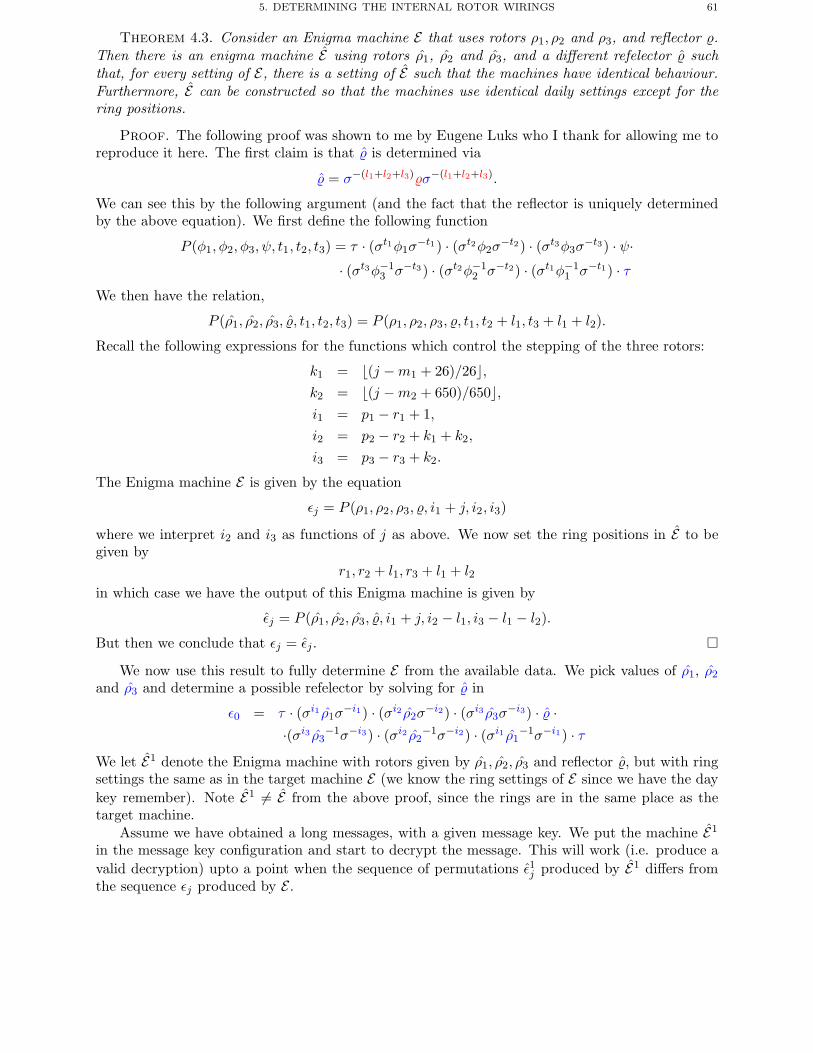
5. DETERMINING THE INTERNAL ROTOR WIRINGS 61
Theorem 4.3. Consider an Enigma machine E that uses rotors ρ1, ρ2 and ρ3, and reflector .Then there is an enigma machine E using rotors ρ1, ρ2 and ρ3, and a different refelector suchthat, for every setting of E, there is a setting of E such that the machines have identical behaviour.Furthermore, E can be constructed so that the machines use identical daily settings except for thering positions.
Proof. The following proof was shown to me by Eugene Luks who I thank for allowing me toreproduce it here. The first claim is that is determined via
= σ−(l1+l2+l3) σ−(l1+l2+l3).
We can see this by the following argument (and the fact that the reflector is uniquely determinedby the above equation). We first define the following function
P (φ1, φ2, φ3, ψ, t1, t2, t3) = τ · (σt1φ1σ−t1) · (σt2φ2σ
−t2) · (σt3φ3σ−t3) · ψ·
· (σt3φ−13 σ−t3) · (σt2φ−1
2 σ−t2) · (σt1φ−11 σ−t1) · τ
We then have the relation,
P (ρ1, ρ2, ρ3, , t1, t2, t3) = P (ρ1, ρ2, ρ3, , t1, t2 + l1, t3 + l1 + l2).
Recall the following expressions for the functions which control the stepping of the three rotors:
k1 = �(j −m1 + 26)/26�,k2 = �(j −m2 + 650)/650�,i1 = p1 − r1 + 1,i2 = p2 − r2 + k1 + k2,
i3 = p3 − r3 + k2.
The Enigma machine E is given by the equation
εj = P (ρ1, ρ2, ρ3, , i1 + j, i2, i3)
where we interpret i2 and i3 as functions of j as above. We now set the ring positions in E to begiven by
r1, r2 + l1, r3 + l1 + l2
in which case we have the output of this Enigma machine is given by
εj = P (ρ1, ρ2, ρ3, , i1 + j, i2 − l1, i3 − l1 − l2).
But then we conclude that εj = εj. �
We now use this result to fully determine E from the available data. We pick values of ρ1, ρ2
and ρ3 and determine a possible refelector by solving for in
ε0 = τ · (σi1 ρ1σ−i1) · (σi2 ρ2σ
−i2) · (σi3 ρ3σ−i3) · ·
·(σi3 ρ3−1σ−i3) · (σi2 ρ2
−1σ−i2) · (σi1 ρ1−1σ−i1) · τ
We let E1 denote the Enigma machine with rotors given by ρ1, ρ2, ρ3 and reflector , but with ringsettings the same as in the target machine E (we know the ring settings of E since we have the daykey remember). Note E1 �= E from the above proof, since the rings are in the same place as thetarget machine.
Assume we have obtained a long messages, with a given message key. We put the machine E1
in the message key configuration and start to decrypt the message. This will work (i.e. produce avalid decryption) upto a point when the sequence of permutations ε1j produced by E1 differs fromthe sequence εj produced by E .
62 4. THE ENIGMA MACHINE
At this point we cycle through all values of l1 and fix the first permutation (and also theassociated reflector) to obtain a new Enigma machine E2 which allows us to decrypt more of thelong message. If a long enough message is obtained we can also obtain l2 is this way, or alternativelywait for another day when the rotors order is changed.
Thus the entire internal workings of the Enigma machine can be determined.
6. Determining The Day Settings
Now having determined the internal wirings, given the set of two months of day settings obtainedby Bertrand, the next task is to determine the actual key when the day settings are not available.At this stage we assume the Germans are still using the encrypt the message setting twice routine.
The essential trick here is to notice that if we write the cipher as
εj = τ · γj · τ ,then
εj · εj+3 = τ · γj · γj+3 · τ .So εj · εj+3 is conjugate to γj · γj+3 and so by Theorem 4.1 they have the same cycle structure.More importantly the cycle structure does not depend on the plug board τ .
Hence, if we can use the cycle structure to determine the rotor settings then we are only leftwith determining the plugboard settings. If we can determine the rotor settings then we know thevalues of γj , for j = 1, . . . , 6, from the encrypted message keys we can compute εj for j = 1, . . . , 6as in the previous section. Hence, determining the plugboard settings is then a question of solvingone of our conjugacy problems again, for τ . But this is easier than before as we have that τ mustbe a product of disjoint transpositions.
We have already discussed how to compute εj · εj+3 from the encryption of the message keys.Hence, we simply compute these values and compare their cycle structures with those obtained byrunning through all possible
60 · 263 · 263 = 18, 534, 946, 560choices for the rotors, positions and ring settings. Note, that when this was done by the Poles inthe 1930’s there was only a choice of the ordering of three rotors. The extra choice of rotors didnot come in till a bit later. Hence, the total choice was 10 times less than this figure.
The above simplifies further if we assume that no stepping of the second and third rotor occursduring the calculation of the first six ciphertext characters. Recall this happens around 77 percentof the time. In such a situation the cycle structure depends only on the rotor order and thedifference pi− ri between the starting rotor position and the ring setting. Hence, we might as wellassume that r1 = r2 = r3 = 0 when computing all of the cycle structures. So, for 77 percent of thedays our search amongst the cycle structures is then only among
60 · 263 = 1, 054, 560 (resp. 105, 456)
possible cycle structures.After the above procedure we have determined all values of the initial day setting bar pi and
ri, however we know the differences pi − ri. We also know for any given message the message keyp′1, p′2, p′3. Hence, in breaking the actual message we only require the solution for r1, r2, the valuefor r3 is irrelevant as the third rotor never moves a fourth rotor. Most German messages startedwith the same two letter word followed by space (space was encoded by ’X’). Hence, we only needto go through 262 different positions to get the correct ring setting. Actually one goes through 262
wheel positions with a fixed ring, and use the differences to infer the actual ring settings.Once, ri is determined from one message the value of pi can be determined for the day key
and then all messages can be trivially broken. Another variant here, if a suitable piece of knownplaintext can be deduced, is to apply the technique from Section 3.2.1 with the obvious modificationto deduce the ring settings as well.
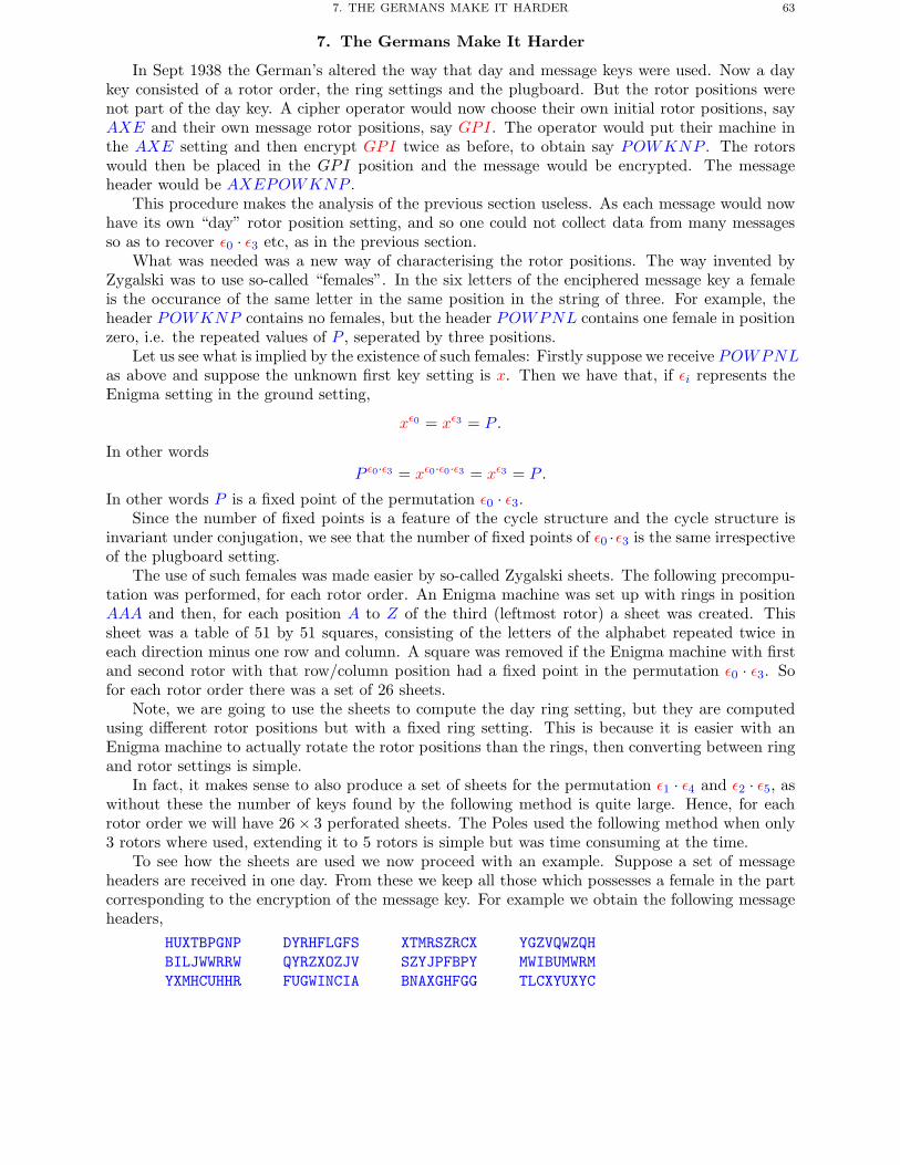
7. THE GERMANS MAKE IT HARDER 63
7. The Germans Make It Harder
In Sept 1938 the German’s altered the way that day and message keys were used. Now a daykey consisted of a rotor order, the ring settings and the plugboard. But the rotor positions werenot part of the day key. A cipher operator would now choose their own initial rotor positions, sayAXE and their own message rotor positions, say GPI. The operator would put their machine inthe AXE setting and then encrypt GPI twice as before, to obtain say POWKNP . The rotorswould then be placed in the GPI position and the message would be encrypted. The messageheader would be AXEPOWKNP .
This procedure makes the analysis of the previous section useless. As each message would nowhave its own “day” rotor position setting, and so one could not collect data from many messagesso as to recover ε0 · ε3 etc, as in the previous section.
What was needed was a new way of characterising the rotor positions. The way invented byZygalski was to use so-called “females”. In the six letters of the enciphered message key a femaleis the occurance of the same letter in the same position in the string of three. For example, theheader POWKNP contains no females, but the header POWPNL contains one female in positionzero, i.e. the repeated values of P , seperated by three positions.
Let us see what is implied by the existence of such females: Firstly suppose we receive POWPNLas above and suppose the unknown first key setting is x. Then we have that, if εi represents theEnigma setting in the ground setting,
xε0 = xε3 = P .
In other wordsP ε0·ε3 = xε0·ε0·ε3 = xε3 = P .
In other words P is a fixed point of the permutation ε0 · ε3.Since the number of fixed points is a feature of the cycle structure and the cycle structure is
invariant under conjugation, we see that the number of fixed points of ε0 ·ε3 is the same irrespectiveof the plugboard setting.
The use of such females was made easier by so-called Zygalski sheets. The following precompu-tation was performed, for each rotor order. An Enigma machine was set up with rings in positionAAA and then, for each position A to Z of the third (leftmost rotor) a sheet was created. Thissheet was a table of 51 by 51 squares, consisting of the letters of the alphabet repeated twice ineach direction minus one row and column. A square was removed if the Enigma machine with firstand second rotor with that row/column position had a fixed point in the permutation ε0 · ε3. Sofor each rotor order there was a set of 26 sheets.
Note, we are going to use the sheets to compute the day ring setting, but they are computedusing different rotor positions but with a fixed ring setting. This is because it is easier with anEnigma machine to actually rotate the rotor positions than the rings, then converting between ringand rotor settings is simple.
In fact, it makes sense to also produce a set of sheets for the permutation ε1 · ε4 and ε2 · ε5, aswithout these the number of keys found by the following method is quite large. Hence, for eachrotor order we will have 26 × 3 perforated sheets. The Poles used the following method when only3 rotors where used, extending it to 5 rotors is simple but was time consuming at the time.
To see how the sheets are used we now proceed with an example. Suppose a set of messageheaders are received in one day. From these we keep all those which possesses a female in the partcorresponding to the encryption of the message key. For example we obtain the following messageheaders,
HUXTBPGNP DYRHFLGFS XTMRSZRCX YGZVQWZQHBILJWWRRW QYRZXOZJV SZYJPFBPY MWIBUMWRMYXMHCUHHR FUGWINCIA BNAXGHFGG TLCXYUXYC
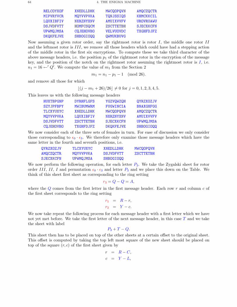
64 4. THE ENIGMA MACHINE
RELCOYXOF XNEDLLDHK MWCQOPQVN AMQCZQCTRMIPVRYVCR MQYVVPVKA TQNJSSIQS KHMCKKCILLQUXIBFIV NXRZNYXNV AMUIXVVFV UROVRUAWUDSJVDFVTT HOMFCSQCM ZSCTTETBH SJECXKCFNUPWMQJMSA CQJEHOVBO VELVUOVDC TXGHFDJFZDKQKFEJVE SHBOGIOQQ QWMUKBUVG
Now assuming a given rotor order, say the rightmost rotor is rotor I, the middle one rotor IIand the leftmost rotor is III, we remove all those headers which could have had a stepping actionof the middle rotor in the first six encryptions. To compute these we take third character of theabove message headers, i.e. the position p1 of the rightmost rotor in the encryption of the messagekey, and the position of the notch on the rightmost rotor assuming the rightmost rotor is I, i.e.n1 = 16 ←′ Q′. We compute the value of m1 from the Section 2
m1 = n1 − p1 − 1 (mod 26).
and remove all those for which
�(j −m1 + 26)/26� �= 0 for j = 0, 1, 2, 3, 4, 5.
This leaves us with the following message headersHUXTBPGNP DYRHFLGFS YGZVQWZQH QYRZXOZJVSZYJPFBPY MWIBUMWRM FUGWINCIA BNAXGHFGGTLCXYUXYC XNEDLLDHK MWCQOPQVN AMQCZQCTRMQYVVPVKA LQUXIBFIV NXRZNYXNV AMUIXVVFVDSJVDFVTT ZSCTTETBH SJECXKCFN UPWMQJMSACQJEHOVBO TXGHFDJFZ DKQKFEJVE SHBOGIOQQ
We now consider each of the three sets of females in turn. For ease of discussion we only considerthose corresponding to ε0 · ε3. We therefore only examine those message headers which have thesame letter in the fourth and seventh positions, i.e.
QYRZXOZJV TLCXYUXYC XNEDLLDHK MWCQOPQVNAMQCZQCTR MQYVVPVKA DSJVDFVTT ZSCTTETBHSJECXKCFN UPWMQJMSA SHBOGIOQQ
We now perform the following operation, for each letter P3. We take the Zygalski sheet for rotororder III, II, I and permutation ε0 · ε3 and letter P3 and we place this down on the Table. Wethink of this sheet first sheet as corresponding to the ring setting
r3 = Q−Q = A,
where the Q comes from the first letter in the first message header. Each row r and column c ofthe first sheet corresponds to the ring setting
r1 = R− r,
r2 = Y − c.
We now take repeat the following process for each message header with a first letter which we havenot yet met before. We take the first letter of the next message header, in this case T and we takethe sheet with label
P3 + T −Q.
This sheet then has to be placed on top of the other sheets at a certain offset to the original sheet.This offset is computed by taking the top left most square of the new sheet should be placed ontop of the square (r, c) of the first sheet given by
r = R− C,
c = Y − L,
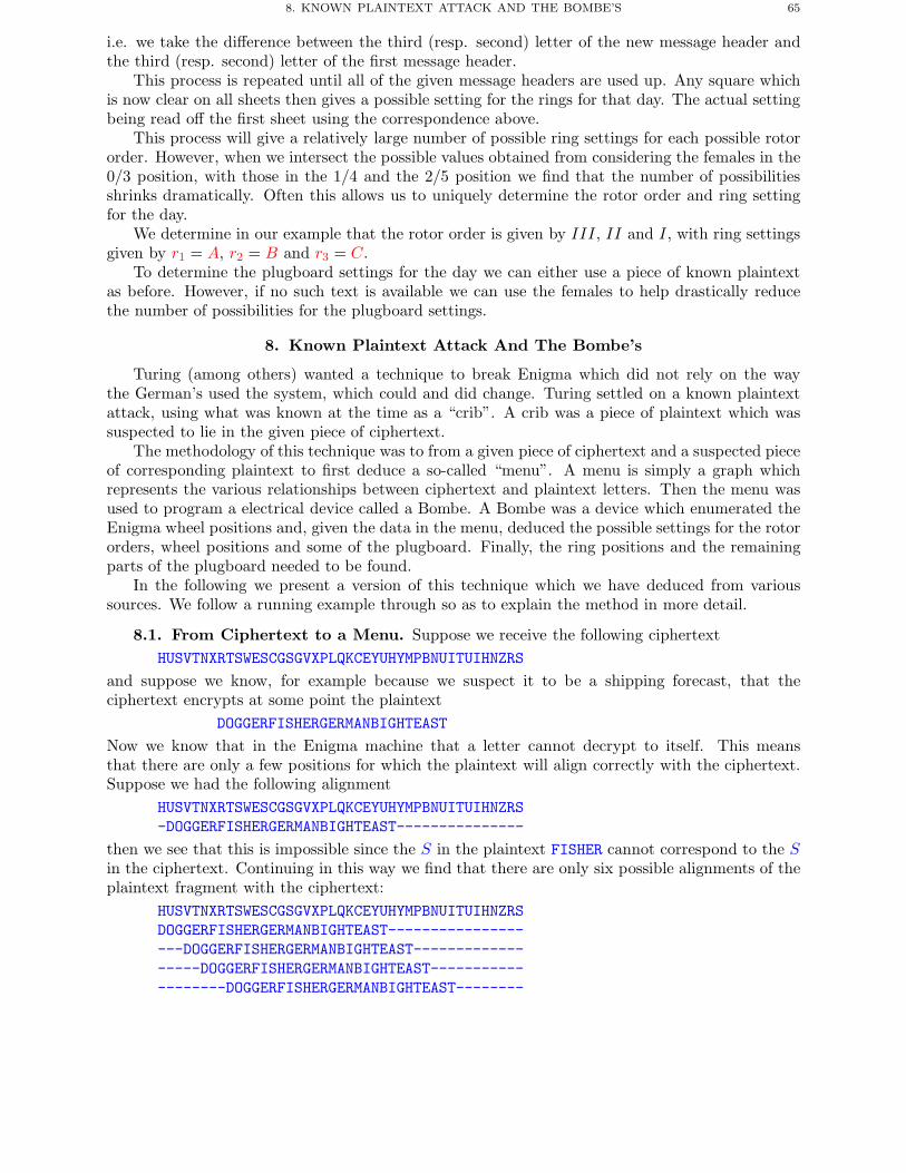
8. KNOWN PLAINTEXT ATTACK AND THE BOMBE’S 65
i.e. we take the difference between the third (resp. second) letter of the new message header andthe third (resp. second) letter of the first message header.
This process is repeated until all of the given message headers are used up. Any square whichis now clear on all sheets then gives a possible setting for the rings for that day. The actual settingbeing read off the first sheet using the correspondence above.
This process will give a relatively large number of possible ring settings for each possible rotororder. However, when we intersect the possible values obtained from considering the females in the0/3 position, with those in the 1/4 and the 2/5 position we find that the number of possibilitiesshrinks dramatically. Often this allows us to uniquely determine the rotor order and ring settingfor the day.
We determine in our example that the rotor order is given by III, II and I, with ring settingsgiven by r1 = A, r2 = B and r3 = C.
To determine the plugboard settings for the day we can either use a piece of known plaintextas before. However, if no such text is available we can use the females to help drastically reducethe number of possibilities for the plugboard settings.
8. Known Plaintext Attack And The Bombe’s
Turing (among others) wanted a technique to break Enigma which did not rely on the waythe German’s used the system, which could and did change. Turing settled on a known plaintextattack, using what was known at the time as a “crib”. A crib was a piece of plaintext which wassuspected to lie in the given piece of ciphertext.
The methodology of this technique was to from a given piece of ciphertext and a suspected pieceof corresponding plaintext to first deduce a so-called “menu”. A menu is simply a graph whichrepresents the various relationships between ciphertext and plaintext letters. Then the menu wasused to program a electrical device called a Bombe. A Bombe was a device which enumerated theEnigma wheel positions and, given the data in the menu, deduced the possible settings for the rotororders, wheel positions and some of the plugboard. Finally, the ring positions and the remainingparts of the plugboard needed to be found.
In the following we present a version of this technique which we have deduced from varioussources. We follow a running example through so as to explain the method in more detail.
8.1. From Ciphertext to a Menu. Suppose we receive the following ciphertextHUSVTNXRTSWESCGSGVXPLQKCEYUHYMPBNUITUIHNZRS
and suppose we know, for example because we suspect it to be a shipping forecast, that theciphertext encrypts at some point the plaintext
DOGGERFISHERGERMANBIGHTEAST
Now we know that in the Enigma machine that a letter cannot decrypt to itself. This meansthat there are only a few positions for which the plaintext will align correctly with the ciphertext.Suppose we had the following alignment
HUSVTNXRTSWESCGSGVXPLQKCEYUHYMPBNUITUIHNZRS-DOGGERFISHERGERMANBIGHTEAST---------------
then we see that this is impossible since the S in the plaintext FISHER cannot correspond to the Sin the ciphertext. Continuing in this way we find that there are only six possible alignments of theplaintext fragment with the ciphertext:
HUSVTNXRTSWESCGSGVXPLQKCEYUHYMPBNUITUIHNZRSDOGGERFISHERGERMANBIGHTEAST-------------------DOGGERFISHERGERMANBIGHTEAST------------------DOGGERFISHERGERMANBIGHTEAST-------------------DOGGERFISHERGERMANBIGHTEAST--------
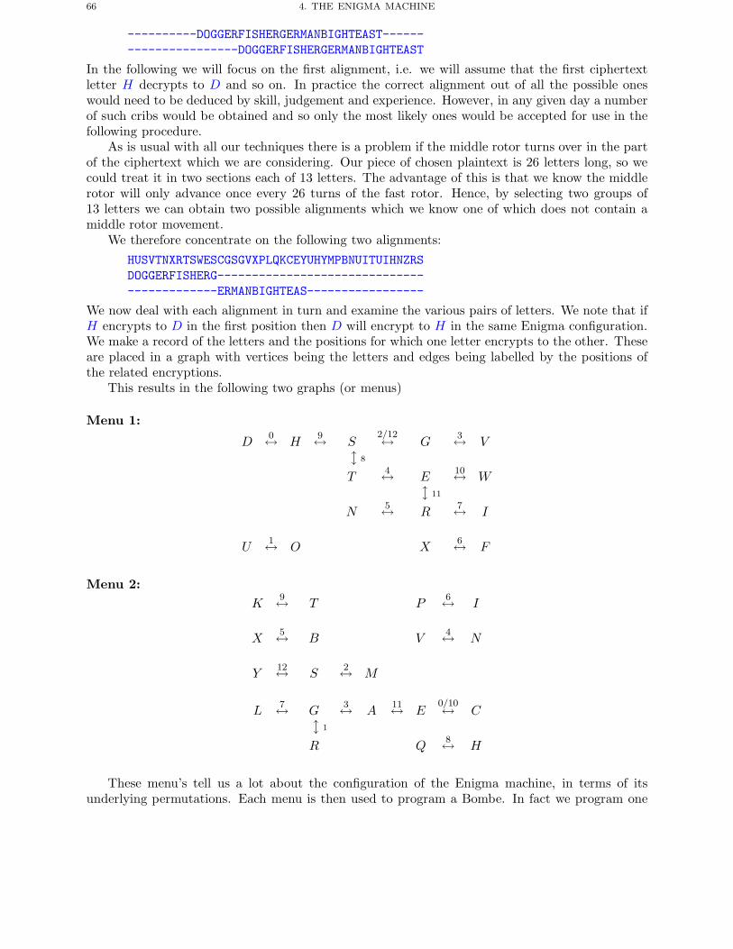
66 4. THE ENIGMA MACHINE
----------DOGGERFISHERGERMANBIGHTEAST----------------------DOGGERFISHERGERMANBIGHTEAST
In the following we will focus on the first alignment, i.e. we will assume that the first ciphertextletter H decrypts to D and so on. In practice the correct alignment out of all the possible oneswould need to be deduced by skill, judgement and experience. However, in any given day a numberof such cribs would be obtained and so only the most likely ones would be accepted for use in thefollowing procedure.
As is usual with all our techniques there is a problem if the middle rotor turns over in the partof the ciphertext which we are considering. Our piece of chosen plaintext is 26 letters long, so wecould treat it in two sections each of 13 letters. The advantage of this is that we know the middlerotor will only advance once every 26 turns of the fast rotor. Hence, by selecting two groups of13 letters we can obtain two possible alignments which we know one of which does not contain amiddle rotor movement.
We therefore concentrate on the following two alignments:HUSVTNXRTSWESCGSGVXPLQKCEYUHYMPBNUITUIHNZRSDOGGERFISHERG-------------------------------------------ERMANBIGHTEAS-----------------
We now deal with each alignment in turn and examine the various pairs of letters. We note that ifH encrypts to D in the first position then D will encrypt to H in the same Enigma configuration.We make a record of the letters and the positions for which one letter encrypts to the other. Theseare placed in a graph with vertices being the letters and edges being labelled by the positions ofthe related encryptions.
This results in the following two graphs (or menus)
Menu 1:
D0↔ H
9↔ S2/12↔ G
3↔ V� 8
T4↔ E
10↔ W� 11
N5↔ R
7↔ I
U1↔ O X
6↔ F
Menu 2:K
9↔ T P6↔ I
X5↔ B V
4↔ N
Y12↔ S
2↔ M
L7↔ G
3↔ A11↔ E
0/10↔ C� 1
R Q8↔ H
These menu’s tell us a lot about the configuration of the Enigma machine, in terms of itsunderlying permutations. Each menu is then used to program a Bombe. In fact we program one
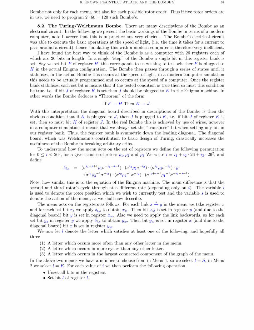
8. KNOWN PLAINTEXT ATTACK AND THE BOMBE’S 67
Bombe not only for each menu, but also for each possible rotor order. Thus if five rotor orders arein use, we need to program 2 · 60 = 120 such Bombe’s.
8.2. The Turing/Welchmann Bombe. There are many descriptions of the Bombe as anelectrical circuit. In the following we present the basic workings of the Bombe in terms of a moderncomputer, note however that this is in practice not very efficient. The Bombe’s electrical circuitwas able to execute the basic operations at the speed of light, (i.e. the time it takes for a current topass around a circuit), hence simulating this with a modern computer is therefore very inefficient.
I have found the best way to think of the Bombe is as a computer with 26 registers each ofwhich are 26 bits in length. In a single “step” of the Bombe a single bit in this register bank isset. Say we set bit F of register H, this corresponds to us wishing to test whether F is plugged toH in the actual Enigma configuration. The Bombe then passes through a series of states until itstabilises, in the actual Bombe this occurs at the speed of light, in a modern computer simulationthis needs to be actually programmed and so occurs at the speed of a computer. Once the registerbank stabilises, each set bit is means that if the tested condition is true then so must this conditionbe true, i.e. if bit J of register K is set then J should be plugged to K in the Enigma machine. Inother words the Bombe deduces a “Theorem” of the form
If F → H Then K → J.
With this interpretation the diagonal board described in descriptions of the Bombe is then theobvious condition that if K is plugged to J , then J is plugged to K, i.e. if bit J of register K isset, then so must bit K of register J . In the real Bombe this is achieved by use of wires, howeverin a computer simulation it means that we always set the “transpose” bit when setting any bit inour register bank. Thus, the register bank is symmetric down the leading diagonal. The diagonalboard, which was Welchmann’s contribution to basic design of Turing, drastically increases theusefulness of the Bombe in breaking arbitrary cribs.
To understand how the menu acts on the set of registers we define the following permutationfor 0 ≤ i < 263, for a given choice of rotors ρ1, ρ2 and ρ3 We write i = i1 + i2 · 26 + i3 · 262, anddefine
δi,s = (σi1+s+1ρ1σ−i1−s−1) · (σi2ρ2σ
−i2) · (σi3ρ3σ−i3) · ·
·(σi3ρ3−1σ−i3) · (σi2ρ2
−1σ−i2) · (σi1+s+1ρ1−1σ−i1−s−1).
Note, how similar this is to the equation of the Enigma machine. The main difference is that thesecond and third rotor’s cycle through at a different rate (depending only on i). The variable iis used to denote the rotor position which we wish to currently test and the variable s is used todenote the action of the menu, as we shall now describe.
The menu acts on the registers as follows: For each link x s→ y in the menu we take register xand for each set bit xz we apply δi,s to obtain xw. Then bit xw is set in register y (and due to thediagonal board) bit y is set in register xw. Also we need to apply the link backwords, so for eachset bit yz in register y we apply δi,s to obtain yw. Then bit yw is set in register x (and due to thediagonal board) bit x is set in register yw.
We now let l denote the letter which satisfies at least one of the following, and hopefully allthree
(1) A letter which occurs more often than any other letter in the menu.(2) A letter which occurs in more cycles than any other letter.(3) A letter which occurs in the largest connected component of the graph of the menu.
In the above two menus we have a number to choose from in Menu 1, so we select l = S, in Menu2 we select l = E. For each value of i we then perform the following operation
• Unset all bits in the registers.• Set bit l of register l.
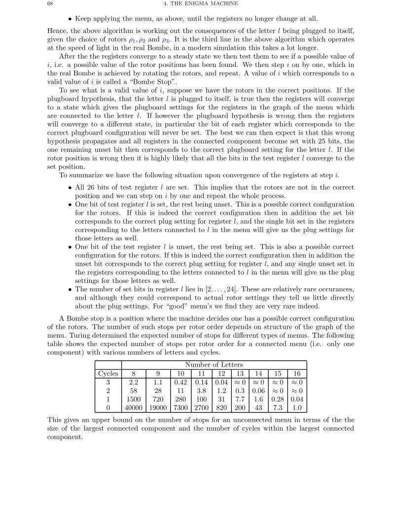
68 4. THE ENIGMA MACHINE
• Keep applying the menu, as above, until the registers no longer change at all.
Hence, the above algorithm is working out the consequences of the letter l being plugged to itself,given the choice of rotors ρ1, ρ2 and ρ3. It is the third line in the above algorithm which operatesat the speed of light in the real Bombe, in a modern simulation this takes a lot longer.
After the the registers converge to a steady state we then test them to see if a possible value ofi, i.e. a possible value of the rotor positions has been found. We then step i on by one, which inthe real Bombe is achieved by rotating the rotors, and repeat. A value of i which corresponds to avalid value of i is called a “Bombe Stop”.
To see what is a valid value of i, suppose we have the rotors in the correct positions. If theplugboard hypothesis, that the letter l is plugged to itself, is true then the registers will convergeto a state which gives the plugboard settings for the registers in the graph of the menu whichare connected to the letter l. If however the plugboard hypothesis is wrong then the registerswill converge to a different state, in particular the bit of each register which corresponds to thecorrect plugboard configuration will never be set. The best we can then expect is that this wronghypothesis propagates and all registers in the connected component become set with 25 bits, theone remaining unset bit then corresponds to the correct plugboard setting for the letter l. If therotor position is wrong then it is highly likely that all the bits in the test register l converge to theset position.
To summarize we have the following situation upon convergence of the registers at step i.
• All 26 bits of test register l are set. This implies that the rotors are not in the correctposition and we can step on i by one and repeat the whole process.
• One bit of test register l is set, the rest being unset. This is a possible correct configurationfor the rotors. If this is indeed the correct configuration then in addition the set bitcorresponds to the correct plug setting for register l, and the single bit set in the registerscorresponding to the letters connected to l in the menu will give us the plug settings forthose letters as well.
• One bit of the test register l is unset, the rest being set. This is also a possible correctconfiguration for the rotors. If this is indeed the correct configuration then in addition theunset bit corresponds to the correct plug setting for register l, and any single unset set inthe registers corresponding to the letters connected to l in the menu will give us the plugsettings for those letters as well.
• The number of set bits in register l lies in [2, . . . , 24]. These are relatively rare occurances,and although they could correspond to actual rotor settings they tell us little directlyabout the plug settings. For “good” menu’s we find they are very rare indeed.
A Bombe stop is a position where the machine decides one has a possible correct configurationof the rotors. The number of such stops per rotor order depends on structure of the graph of themenu. Turing determined the expected number of stops for different types of menus. The followingtable shows the expected number of stops per rotor order for a connected menu (i.e. only onecomponent) with various numbers of letters and cycles.
Number of LettersCycles 8 9 10 11 12 13 14 15 16
3 2.2 1.1 0.42 0.14 0.04 ≈ 0 ≈ 0 ≈ 0 ≈ 02 58 28 11 3.8 1.2 0.3 0.06 ≈ 0 ≈ 01 1500 720 280 100 31 7.7 1.6 0.28 0.040 40000 19000 7300 2700 820 200 43 7.3 1.0
This gives an upper bound on the number of stops for an unconnected menu in terms of the thesize of the largest connected component and the number of cycles within the largest connectedcomponent.
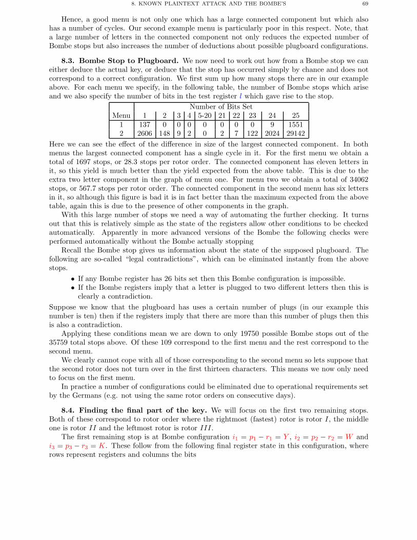
8. KNOWN PLAINTEXT ATTACK AND THE BOMBE’S 69
Hence, a good menu is not only one which has a large connected component but which alsohas a number of cycles. Our second example menu is particularly poor in this respect. Note, thata large number of letters in the connected component not only reduces the expected number ofBombe stops but also increases the number of deductions about possible plugboard configurations.
8.3. Bombe Stop to Plugboard. We now need to work out how from a Bombe stop we caneither deduce the actual key, or deduce that the stop has occurred simply by chance and does notcorrespond to a correct configuration. We first sum up how many stops there are in our exampleabove. For each menu we specify, in the following table, the number of Bombe stops which ariseand we also specify the number of bits in the test register l which gave rise to the stop.
Number of Bits SetMenu 1 2 3 4 5-20 21 22 23 24 25
1 137 0 0 0 0 0 0 0 9 15512 2606 148 9 2 0 2 7 122 2024 29142
Here we can see the effect of the difference in size of the largest connected component. In bothmenus the largest connected component has a single cycle in it. For the first menu we obtain atotal of 1697 stops, or 28.3 stops per rotor order. The connected component has eleven letters init, so this yield is much better than the yield expected from the above table. This is due to theextra two letter component in the graph of menu one. For menu two we obtain a total of 34062stops, or 567.7 stops per rotor order. The connected component in the second menu has six lettersin it, so although this figure is bad it is in fact better than the maximum expected from the abovetable, again this is due to the presence of other components in the graph.
With this large number of stops we need a way of automating the further checking. It turnsout that this is relatively simple as the state of the registers allow other conditions to be checkedautomatically. Apparently in more advanced versions of the Bombe the following checks wereperformed automatically without the Bombe actually stopping
Recall the Bombe stop gives us information about the state of the supposed plugboard. Thefollowing are so-called “legal contradictions”, which can be eliminated instantly from the abovestops.
• If any Bombe register has 26 bits set then this Bombe configuration is impossible.• If the Bombe registers imply that a letter is plugged to two different letters then this is
clearly a contradiction.Suppose we know that the plugboard has uses a certain number of plugs (in our example thisnumber is ten) then if the registers imply that there are more than this number of plugs then thisis also a contradiction.
Applying these conditions mean we are down to only 19750 possible Bombe stops out of the35759 total stops above. Of these 109 correspond to the first menu and the rest correspond to thesecond menu.
We clearly cannot cope with all of those corresponding to the second menu so lets suppose thatthe second rotor does not turn over in the first thirteen characters. This means we now only needto focus on the first menu.
In practice a number of configurations could be eliminated due to operational requirements setby the Germans (e.g. not using the same rotor orders on consecutive days).
8.4. Finding the final part of the key. We will focus on the first two remaining stops.Both of these correspond to rotor order where the rightmost (fastest) rotor is rotor I, the middleone is rotor II and the leftmost rotor is rotor III.
The first remaining stop is at Bombe configuration i1 = p1 − r1 = Y , i2 = p2 − r2 = W andi3 = p3 − r3 = K. These follow from the following final register state in this configuration, whererows represent registers and columns the bits
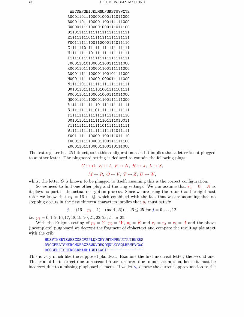
70 4. THE ENIGMA MACHINE
ABCDEFGHIJKLMNOPQRSTUVWXYZA00011011100001000111011000B00011011100001100111111000C00001111100001000111011100D11011111111111111111111111E11111111011111111111111111F00111111100110000111011110G11111101111111111111111111H11111111101111111111111111I11110111111111111111111111J00011010100001100111111000K00011011100001100111111000L00011111100001100101111000M00011111100001000011111000N11111011111111111111111111O01011011111101001111101111P00011011100001000111011000Q00011011100001100111111000R11111111111101111111111111S11111111111011111111111111T11111111111111111111111110U01011011111111101111010011V11111111111111011111111111W11111111111111111111011111X00111111100001100111011110Y00011111100001100111111100Z00011011100001100110111000
The test register has 25 bits set, so in this configuration each bit implies that a letter is not pluggedto another letter. The plugboard setting is deduced to contain the following plugs
C ↔ D, E ↔ I, F ↔ N, H ↔ J, L↔ S,
M ↔ R, O ↔ V , T ↔ Z, U ↔ W,
whilst the letter G is known to be plugged to itself, assuming this is the correct configuration.So we need to find one other plug and the ring settings. We can assume that r3 = 0 = A as
it plays no part in the actual decryption process. Since we are using the rotor I as the rightmostrotor we know that n1 = 16 ← Q, which combined with the fact that we are assuming that nostepping occurs in the first thirteen characters implies that p1 must satisfy
j − ((16 − p1 − 1) (mod 26)) + 26 ≤ 25 for j = 0, . . . , 12.
i.e. p1 = 0, 1, 2, 16, 17, 18, 19, 20, 21, 22, 23, 24 or 25.With the Enigma setting of p1 = Y , p2 = W , p3 = K and r1 = r2 = r3 = A and the above
(incomplete) plugboard we decrypt the fragment of ciphertext and compare the resulting plaintextwith the crib.
HUSVTNXRTSWESCGSGVXPLQKCEYUHYMPBNUITUIHNZRSDVGGERLISHERGMWBRXZSWNVOMQOQKLKCSQLRRHPVCAGDOGGERFISHERGERMANBIGHTEAST----------------
This is very much like the supposed plaintext. Examine the first incorrect letter, the second one.This cannot be incorrect due to a second rotor turnover, due to our assumption, hence it must beincorrect due to a missing plugboard element. If we let γ1 denote the current approximation to the
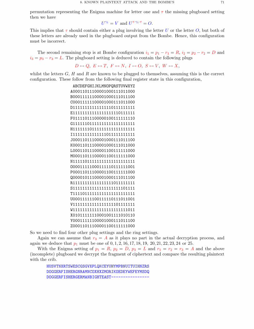
8. KNOWN PLAINTEXT ATTACK AND THE BOMBE’S 71
permutation representing the Enigma machine for letter one and τ the missing plugboard settingthen we have
Uγ1 = V and U τ ·γ1·τ = O.
This implies that τ should contain either a plug involving the letter U or the letter O, but both ofthese letters are already used in the plugboard output from the Bombe. Hence, this configurationmust be incorrect.
The second remaining stop is at Bombe configuration i1 = p1 − r1 = R, i2 = p2 − r2 = D andi3 = p3 − r3 = L. The plugboard setting is deduced to contain the following plugs
D ↔ Q, E ↔ T , F ↔ N, I ↔ O, S ↔ V , W ↔ X,
whilst the letters G, H and R are known to be plugged to themselves, assuming this is the correctconfiguration. These follow from the following final register state in this configuration,
ABCDEFGHIJKLMNOPQRSTUVWXYZA00011011100001000111011000B00011111100001000111011100C00011111100001000111011000D11111111111111110111111111E11111111111111111110111111F01111011100000100111111110G11111101111111111111111111H11111110111111111111111111I11111111111111011111111111J00011011100001000111011100K00011011100001000111011000L00011011100001100111111000M00011011100001100111111000N11111011111111111111111111O00011111000111110111111001P00011011100001100111111000Q00001011100001000111011100R11111111111111111011111111S11111111111111111111101111T11110111111111111111111111U00011111100111110111011001V11111111111111111101111111W11111111111111111111111011X01011111110001001111010110Y00011111100001000111011100Z00011011100001100111111000
So we need to find four other plug settings and the ring settings.Again we can assume that r3 = A as it plays no part in the actual decryption process, and
again we deduce that p1 must be one of 0, 1, 2, 16, 17, 18, 19, 20, 21, 22, 23, 24 or 25.With the Enigma setting of p1 = R, p2 = D, p3 = L and r1 = r2 = r3 = A and the above
(incomplete) plugboard we decrypt the fragment of ciphertext and compare the resulting plaintextwith the crib.
HUSVTNXRTSWESCGSGVXPLQKCEYUHYMPBNUITUIHNZRSDOGGERFISHERGNRAMNCOXHXZMORIKOEDEYWEFEYMSDQDOGGERFISHERGERMANBIGHTEAST----------------
72 4. THE ENIGMA MACHINE
We now look at the first incorrect letter, this is in the 14 position. Using the same notation asbefore, i.e. γj for the current approximation and τ for the missing plugs, we see that if this incorrectoperation is due to a plug problem rather than a rotor turnover problem then we must have
Cτ ·γ13·τ = E.
Now, E already occurs on the plugboard, via E ↔ T , so τ must include a plug which maps C tothe letter x where
xγ13 = E.
But we can compute that
γ13 = (AM)(BE)(CN)(DO)(FI)(GS)(HX)(JU)(KP )(LQ)(RV )(TY )(WZ),
from which we deduce that x = B. So we include the plug C ↔ B in our new approximation andrepeat to obtain the plaintext
HUSVTNXRTSWESCGSGVXPLQKCEYUHYMPBNUITUIHNZRSDOGGERFISHERGERAMNBOXHXNMORIKOEMEYWEFEYMSDQDOGGERFISHERGERMANBIGHTEAST----------------
We then see in the 16th position that we either need to step the rotor or there should be a plugwhich means that S maps to M under the cipher. We have, for our new γ15 that
γ15 = (AS)(BJ)(CY )(DK)(EX)(FW )(GI)(HU)(LM)(NQ)(OP )(RV )(TZ).
The letter S already occurs in a plug, so we must have that A is plugged to M . We add this pluginto our configuration and repeat
HUSVTNXRTSWESCGSGVXPLQKCEYUHYMPBNUITUIHNZRSDOGGERFISHERGERMANBOXHXNAORIKVEAEYWEFEYASDQDOGGERFISHERGERMANBIGHTEAST----------------
Now the 20th character is incorrect, we need that P should map to I and not O under the cipherin this position. Again assuming this is due to a missing plug we find that
γ19 = (AH)(BM)(CF )(DY )(EV )(GX)(IK)(JR)(LS)(NT )(OP )(QW )(UZ).
There is already a plug involving the letter I so we deduce that the missing plug should be K ↔ P .Again we add this new plug into our configuration and repeat to obtain
HUSVTNXRTSWESCGSGVXPLQKCEYUHYMPBNUITUIHNZRSDOGGERFISHERGERMANBIXHJNAORIPVXAEYWEFEYASDQDOGGERFISHERGERMANBIGHTEAST----------------
Now the 21st character is wrong as we must have that L should map to G. We know G is pluggedto itself, from the Bombe stop configuration and given
γ20 = (AI)(BJ)(CW )(DE)(FK)(GZ)(HU)(LX)(MQ)(NT )(OV )(PY )(RS),
we deduce that if this error is due to a plug we must have that L is plugged to Z. We add thisfinal plug into our configuration and find that we obtain
HUSVTNXRTSWESCGSGVXPLQKCEYUHYMPBNUITUIHNZRSDOGGERFISHERGERMANBIGHJNAORIPVXAEYWEFEYAQDQDOGGERFISHERGERMANBIGHTEAST----------------
All the additional plugs we have added have been on the assumption that no rotor turnover hasyet occurred. Any further errors must be due to rotor turnover, as we now have a full set of plugs(as we know our configuration only has ten plugs in use). If when correcting the rotor turnover westill do not decrypt correctly we need to backup and repeat the process.
We see that the next error occurs in position 23. This means that a rotor turnover must haveoccurred just before this letter was encrypted, in other words we have
22 − ((16 − p1 − 1) (mod 26)) + 26 = 26.
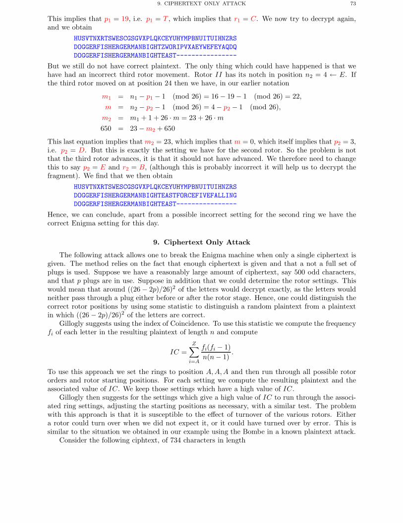
9. CIPHERTEXT ONLY ATTACK 73
This implies that p1 = 19, i.e. p1 = T , which implies that r1 = C. We now try to decrypt again,and we obtain
HUSVTNXRTSWESCGSGVXPLQKCEYUHYMPBNUITUIHNZRSDOGGERFISHERGERMANBIGHTZWORIPVXAEYWEFEYAQDQDOGGERFISHERGERMANBIGHTEAST----------------
But we still do not have correct plaintext. The only thing which could have happened is that wehave had an incorrect third rotor movement. Rotor II has its notch in position n2 = 4 ← E. Ifthe third rotor moved on at position 24 then we have, in our earlier notation
m1 = n1 − p1 − 1 (mod 26) = 16 − 19 − 1 (mod 26) = 22,m = n2 − p2 − 1 (mod 26) = 4 − p2 − 1 (mod 26),m2 = m1 + 1 + 26 ·m = 23 + 26 ·m650 = 23 −m2 + 650
This last equation implies that m2 = 23, which implies that m = 0, which itself implies that p2 = 3,i.e. p2 = D. But this is exactly the setting we have for the second rotor. So the problem is notthat the third rotor advances, it is that it should not have advanced. We therefore need to changethis to say p2 = E and r2 = B, (although this is probably incorrect it will help us to decrypt thefragment). We find that we then obtain
HUSVTNXRTSWESCGSGVXPLQKCEYUHYMPBNUITUIHNZRSDOGGERFISHERGERMANBIGHTEASTFORCEFIVEFALLINGDOGGERFISHERGERMANBIGHTEAST----------------
Hence, we can conclude, apart from a possible incorrect setting for the second ring we have thecorrect Enigma setting for this day.
9. Ciphertext Only Attack
The following attack allows one to break the Enigma machine when only a single ciphertext isgiven. The method relies on the fact that enough ciphertext is given and that a not a full set ofplugs is used. Suppose we have a reasonably large amount of ciphertext, say 500 odd characters,and that p plugs are in use. Suppose in addition that we could determine the rotor settings. Thiswould mean that around ((26 − 2p)/26)2 of the letters would decrypt exactly, as the letters wouldneither pass through a plug either before or after the rotor stage. Hence, one could distinguish thecorrect rotor positions by using some statistic to distinguish a random plaintext from a plaintextin which ((26 − 2p)/26)2 of the letters are correct.
Gillogly suggests using the index of Coincidence. To use this statistic we compute the frequencyfi of each letter in the resulting plaintext of length n and compute
IC =Z∑i=A
fi(fi − 1)n(n− 1)
.
To use this approach we set the rings to position A,A,A and then run through all possible rotororders and rotor starting positions. For each setting we compute the resulting plaintext and theassociated value of IC. We keep those settings which have a high value of IC.
Gillogly then suggests for the settings which give a high value of IC to run through the associ-ated ring settings, adjusting the starting positions as necessary, with a similar test. The problemwith this approach is that it is susceptible to the effect of turnover of the various rotors. Eithera rotor could turn over when we did not expect it, or it could have turned over by error. This issimilar to the situation we obtained in our example using the Bombe in a known plaintext attack.
Consider the following ciphtext, of 734 characters in length
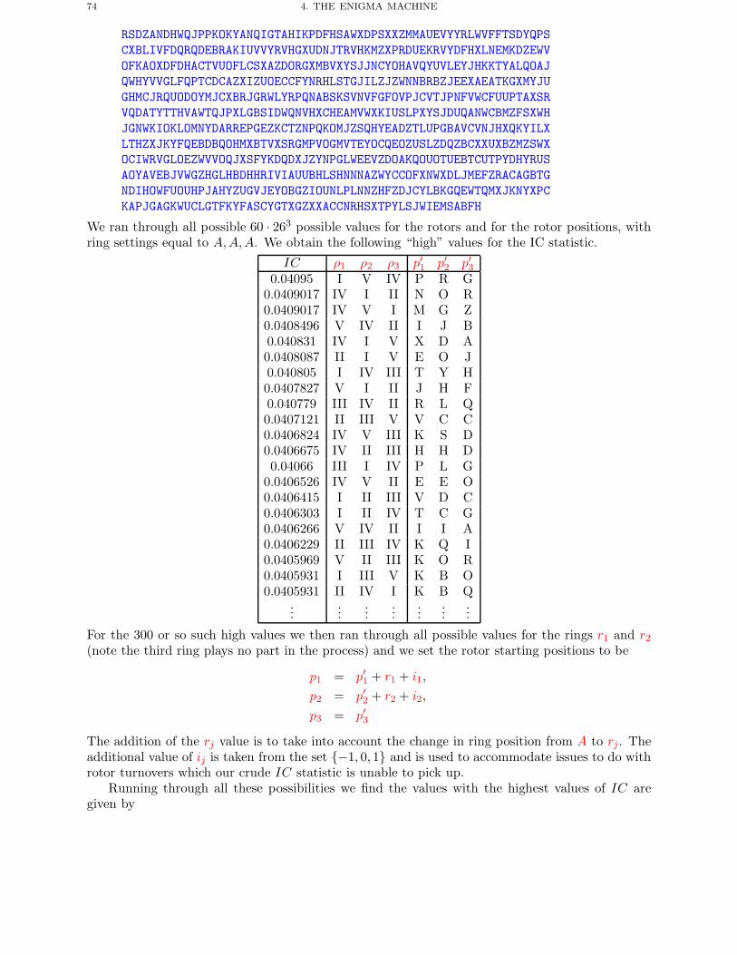
74 4. THE ENIGMA MACHINE
RSDZANDHWQJPPKOKYANQIGTAHIKPDFHSAWXDPSXXZMMAUEVYYRLWVFFTSDYQPSCXBLIVFDQRQDEBRAKIUVVYRVHGXUDNJTRVHKMZXPRDUEKRVYDFHXLNEMKDZEWVOFKAOXDFDHACTVUOFLCSXAZDORGXMBVXYSJJNCYOHAVQYUVLEYJHKKTYALQOAJQWHYVVGLFQPTCDCAZXIZUOECCFYNRHLSTGJILZJZWNNBRBZJEEXAEATKGXMYJUGHMCJRQUODOYMJCXBRJGRWLYRPQNABSKSVNVFGFOVPJCVTJPNFVWCFUUPTAXSRVQDATYTTHVAWTQJPXLGBSIDWQNVHXCHEAMVWXKIUSLPXYSJDUQANWCBMZFSXWHJGNWKIOKLOMNYDARREPGEZKCTZNPQKOMJZSQHYEADZTLUPGBAVCVNJHXQKYILXLTHZXJKYFQEBDBQOHMXBTVXSRGMPVOGMVTEYOCQEOZUSLZDQZBCXXUXBZMZSWXOCIWRVGLOEZWVVOQJXSFYKDQDXJZYNPGLWEEVZDOAKQOUOTUEBTCUTPYDHYRUSAOYAVEBJVWGZHGLHBDHHRIVIAUUBHLSHNNNAZWYCCOFXNWXDLJMEFZRACAGBTGNDIHOWFUOUHPJAHYZUGVJEYOBGZIOUNLPLNNZHFZDJCYLBKGQEWTQMXJKNYXPCKAPJGAGKWUCLGTFKYFASCYGTXGZXXACCNRHSXTPYLSJWIEMSABFH
We ran through all possible 60 · 263 possible values for the rotors and for the rotor positions, withring settings equal to A,A,A. We obtain the following “high” values for the IC statistic.
IC ρ1 ρ2 ρ3 p′1 p′2 p′30.04095 I V IV P R G
0.0409017 IV I II N O R0.0409017 IV V I M G Z0.0408496 V IV II I J B0.040831 IV I V X D A0.0408087 II I V E O J0.040805 I IV III T Y H0.0407827 V I II J H F0.040779 III IV II R L Q0.0407121 II III V V C C0.0406824 IV V III K S D0.0406675 IV II III H H D0.04066 III I IV P L G
0.0406526 IV V II E E O0.0406415 I II III V D C0.0406303 I II IV T C G0.0406266 V IV II I I A0.0406229 II III IV K Q I0.0405969 V II III K O R0.0405931 I III V K B O0.0405931 II IV I K B Q
......
......
......
...
For the 300 or so such high values we then ran through all possible values for the rings r1 and r2(note the third ring plays no part in the process) and we set the rotor starting positions to be
p1 = p′1 + r1 + i1,
p2 = p′2 + r2 + i2,
p3 = p′3
The addition of the rj value is to take into account the change in ring position from A to rj. Theadditional value of ij is taken from the set {−1, 0, 1} and is used to accommodate issues to do withrotor turnovers which our crude IC statistic is unable to pick up.
Running through all these possibilities we find the values with the highest values of IC aregiven by
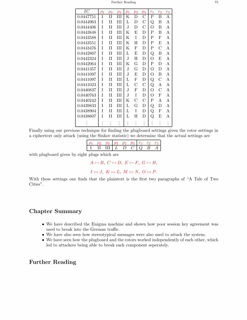
Further Reading 75
IC ρ1 ρ2 ρ3 p1 p2 p3 r1 r2 r30.0447751 I II III K D C P B A0.0444963 I II III L D C Q B A0.0444406 I II III J D C O B A0.0443848 I II III K E D P B A0.0443588 I II III K I D P F A0.0443551 I II III K H D P E A0.0443476 I II III K F D P C A0.0442807 I II III L E D Q B A0.0442324 I II III J H D O E A0.0442064 I II III K G D P D A0.0441357 I II III J G D O D A0.0441097 I II III J E D O B A0.0441097 I II III L F D Q C A0.0441023 I II III L C C Q A A0.0440837 I II III J F D O C A0.0440763 I II III J I D O F A0.0440242 I II III K C C P A A0.0439833 I II III L G D Q D A0.0438904 I II III L I D Q F A0.0438607 I II III L H D Q E A
......
......
......
......
......
Finally using our previous technique for finding the plugboard settings given the rotor settings ina ciphertext only attack (using the Sinkov statistic) we determine that the actual settings are
ρ1 ρ2 ρ3 p1 p2 p3 r1 r2 r3I II III L D C Q B A
with plugboard given by eight plugs which are
A↔ B, C ↔ D, E ↔ F, G↔ H,
I ↔ J, K ↔ L, M ↔ N, O ↔ P .
With these settings one finds that the plaintext is the first two paragraphs of “A Tale of TwoCities”.
Chapter Summary
• We have described the Enigma machine and shown how poor session key agreement wasused to break into the German traffic.
• We have also seen how stereotypical messages were also used to attack the system.• We have seen how the plugboard and the rotors worked independently of each other, which
led to attackers being able to break each component seperately.
Further Reading
76 4. THE ENIGMA MACHINE
The paper by Rejweski presents the work of the Polish cryptographers very clearly. The pureciphertext only attack is presented in the papers by Gillogly and Williams. There are a number ofexcellent sites on the internet which go into various details, of particular note are Tony Sale’s website and the Bletchley Park site.
J. Gillogly. Ciphertext-only cryptanalysis of Enigma. Cryptologia, 14, 1995.
M. Rejewski. An application of the theory of permutations in breaking the Enigma cipher. Appli-cationes Mathematicae, 16, 1980.
H. Williams. Applying statistical language recognition techniques in the ciphertext-only cryptanal-ysis of Enigma. Cryptologia, 24, 2000.
Bletchley Park Web Site. http://www.bletchleypark.org.uk/.
Tony Sale’s Web Site. http://www.codesandciphers.org.uk/.
CHAPTER 5
Information Theoretic Security
Chapter Goals
• To introduce the concept of perfect secrecy.• To discuss the security of the one-time pad.• To introduce the concept of entropy.• To explain the notion of key equivocation, spurious keys and unicity distance.• To use these tools to understand why the prior historical encryption algorithms are weak.
1. Introduction
Information theory is one of the foundations of computer science. In this chapter we will examineits relationship to cryptography. But we shall not assume any prior familiarity with informationtheory.
We first need to overview the difference between information theoretic security and compu-tational security. Informally, a cryptographic system is called computationally secure if the bestpossible algorithm for breaking it requires N operations, where N is such a large number that itis infeasible to carry out this many operations. With current computing power we assume that280 operations is an infeasible number of operations to carry out. Hence, a value of N larger than280 would imply that the system is computationally secure. Notice that no actual system can beproved secure under this definition, since we never know whether there is a better algorithm thanthe one known. Hence, in practice we say a system is computationally secure if the best knownalgorithm for breaking it requires an unreasonably large amount of computational resources.
Another practical approach, related to computational security, is to reduce breaking the systemto solving some well-studied hard problem. For example, we can try to show that a given systemis secure if a given integer N cannot be factored. Systems of this form are often called provablysecure. However, we only have a proof relative to some hard problem, hence this does not providean absolute proof.
Essentially, a computationally secure scheme, or one which is provably secure, is only securewhen we consider an adversary whose computational resources are bounded. Even if the adversaryhas large, but limited, resources she still will not break the system.
When considering schemes which are computationally secure we need to be very clear aboutcertain issues:
• We need to be careful about the key sizes etc. If the key size is small then our adversarymay have enough computational resources to break the system.
• We need to keep abreast of current algorithmic developments and developments in com-puter hardware.
• At some point in the future we should expect our system to become broken, either throughan improvement in computing power or an algorithmic breakthrough.
77
78 5. INFORMATION THEORETIC SECURITY
It turns out that most schemes in use today are computationally secure, and so every chapter inthis book (except this one) will solely be interested in computationally secure systems.
On the other hand, a system is said to be unconditionally secure when we place no limit on thecomputational power of the adversary. In other words a system is unconditionally secure if it cannotbe broken even with infinite computing power. Hence, no matter what algorithmic improvementsare made or what improvements in computing technology occur, an unconditionally secure schemewill never be broken. Other names for unconditional security you find in the literature are perfectsecurity or information theoretic security.
You have already seen that the following systems are not computationally secure, since wealready know how to break them with very limited computing resources:
• shift cipher,• substitution cipher,• Vigenere cipher.
Of the systems we shall meet later, the following are computationally secure but are not uncondi-tionally secure:
• DES and Rijndael,• RSA,• ElGamal encryption.
However, the one-time pad which we shall meet in this chapter is unconditionally secure, but onlyif it is used correctly.
2. Probability and Ciphers
Before we can introduce formally the concept of unconditional security we first need to under-stand in more detail the role of probability in understanding simple ciphers. We make the followingdefinitions:
• Let P denote the set of possible plaintexts.• Let K denote the set of possible keys.• Let C denote the set of ciphertexts.
Each of these can be thought of as a probability distribution, where we denote the probabilities byp(P = m), p(K = k), p(C = c).
So for example, if our message space is P = {a, b, c} and the message a occurs with probability1/4 then we write
p(P = a) =14.
We make the reasonable assumption that P and K are independent, i.e. the user will not decide toencrypt certain messages under one key and other messages under another. The set of ciphertextsunder a specific key k is defined by
C(k) = {ek(x) : x ∈ P},where the encryption function is defined by ek(m). We then have the relationship
(7) p(C = c) =∑
k:c∈C(k)
p(K = k) · p(P = dk(c)),
where the decryption function is defined by dk(c). As an example, which we shall use throughoutthis section, assume that we have only four messages P = {a, b, c, d} which occur with probability
• p(P = a) = 1/4,• p(P = b) = 3/10,• p(P = c) = 3/20,• p(P = d) = 3/10.
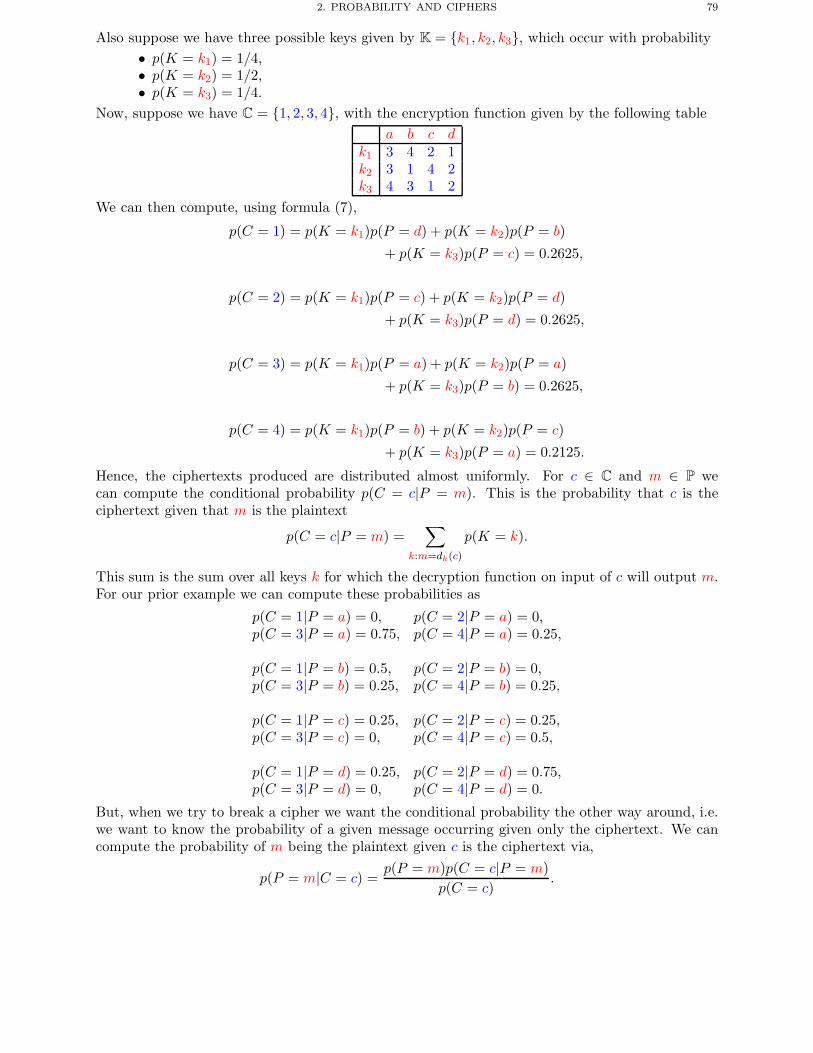
2. PROBABILITY AND CIPHERS 79
Also suppose we have three possible keys given by K = {k1, k2, k3}, which occur with probability• p(K = k1) = 1/4,• p(K = k2) = 1/2,• p(K = k3) = 1/4.
Now, suppose we have C = {1, 2, 3, 4}, with the encryption function given by the following tablea b c d
k1 3 4 2 1k2 3 1 4 2k3 4 3 1 2
We can then compute, using formula (7),
p(C = 1) = p(K = k1)p(P = d) + p(K = k2)p(P = b)
+ p(K = k3)p(P = c) = 0.2625,
p(C = 2) = p(K = k1)p(P = c) + p(K = k2)p(P = d)
+ p(K = k3)p(P = d) = 0.2625,
p(C = 3) = p(K = k1)p(P = a) + p(K = k2)p(P = a)
+ p(K = k3)p(P = b) = 0.2625,
p(C = 4) = p(K = k1)p(P = b) + p(K = k2)p(P = c)
+ p(K = k3)p(P = a) = 0.2125.
Hence, the ciphertexts produced are distributed almost uniformly. For c ∈ C and m ∈ P wecan compute the conditional probability p(C = c|P = m). This is the probability that c is theciphertext given that m is the plaintext
p(C = c|P = m) =∑
k:m=dk(c)
p(K = k).
This sum is the sum over all keys k for which the decryption function on input of c will output m.For our prior example we can compute these probabilities as
p(C = 1|P = a) = 0, p(C = 2|P = a) = 0,p(C = 3|P = a) = 0.75, p(C = 4|P = a) = 0.25,
p(C = 1|P = b) = 0.5, p(C = 2|P = b) = 0,p(C = 3|P = b) = 0.25, p(C = 4|P = b) = 0.25,
p(C = 1|P = c) = 0.25, p(C = 2|P = c) = 0.25,p(C = 3|P = c) = 0, p(C = 4|P = c) = 0.5,
p(C = 1|P = d) = 0.25, p(C = 2|P = d) = 0.75,p(C = 3|P = d) = 0, p(C = 4|P = d) = 0.
But, when we try to break a cipher we want the conditional probability the other way around, i.e.we want to know the probability of a given message occurring given only the ciphertext. We cancompute the probability of m being the plaintext given c is the ciphertext via,
p(P = m|C = c) =p(P = m)p(C = c|P = m)
p(C = c).
80 5. INFORMATION THEORETIC SECURITY
This conditional probability can be computed by anyone who knows the encryption function andthe probability distributions of K and P . Using these probabilities one may be able to deduce someinformation about the plaintext once you have seen the ciphertext.
Returning to our previous example we compute
p(P = a|C = 1) = 0, p(P = b|C = 1) = 0.571,p(P = c|C = 1) = 0.143, p(P = d|C = 1) = 0.286,
p(P = a|C = 2) = 0, p(P = b|C = 2) = 0,p(P = c|C = 2) = 0.143, p(P = d|C = 2) = 0.857,
p(P = a|C = 3) = 0.714, p(P = b|C = 3) = 0.286,p(P = c|C = 3) = 0, p(P = d|C = 3) = 0,
p(P = a|C = 4) = 0.294, p(P = b|C = 4) = 0.352,p(P = c|C = 4) = 0.352, p(P = d|C = 4) = 0.
Hence• If we see the ciphertext 1 then we know the message is not equal to a. We also can guess
that it is more likely to be b rather than c or d.• If we see the ciphertext 2 then we know the message is not equal to a or b. We also can
be pretty certain that the message is equal to d.• If we see the ciphertext 3 then we know the message is not equal to c or d and have a good
chance that it is equal to a.• If we see the ciphertext 4 then we know the message is not equal to d, but cannot really
guess with certainty as to whether the message is a, b or c.So in our previous example the ciphertext does reveal a lot of information about the plaintext. Butthis is exactly what we wish to avoid, we want the ciphertext to give no information about theplaintext.
A system with this property, that the ciphertext reveals nothing about the plaintext, is said tobe perfectly secure.
Definition 5.1 (Perfect Secrecy). A cryptosystem has perfect secrecy if
p(P = m|C = c) = p(P = m)
for all plaintexts m and all ciphertexts c.
This means the probability that the plaintext is m, given that you know the ciphertext is c,is the same as the probability that it is m without seeing c. In other words knowing c reveals noinformation about m. Another way of describing perfect secrecy is via:
Lemma 5.2. A cryptosystem has perfect secrecy if p(C = c|P = m) = p(C = c) for all m andc.
Proof. This trivially follows from the definition
p(P = m|C = c) =p(P = m)p(C = c|P = m)
p(C = c)and the fact that perfect secrecy means p(P = m|C = c) = p(P = m). �
The first result about a perfect security is
Lemma 5.3. Assume the cryptosystem is perfectly secure, then
#K ≥ #C ≥ #P,
where
2. PROBABILITY AND CIPHERS 81
• #K denotes the size of the set of possible keys,• #C denotes the size of the set of possible ciphertexts,• #P denotes the size of the set of possible plaintexts.
Proof. First note that in any encryption scheme, we must have
#C ≥ #P
since encryption must be an injective map.We assume that every ciphertext can occur, i.e. p(C = c) > 0 for all c ∈ C, since if this does
not hold then we can alter our definition of C. Then for any message m and any ciphertext c wehave
p(C = c|P = m) = p(C = c) > 0.
This means for each m, that for all c there must be a key k such that
ek(m) = c.
Hence, #K ≥ #C as required. �
We now come to the main theorem due to Shannon on perfectly secure ciphers. Shannon’sTheorem tells us exactly which encryption schemes are perfectly secure and which are not.
Theorem 5.4 (Shannon). Let(P,C,K, ek(·), dk(·))
denote a cryptosystem with #P = #C = #K. Then the cryptosystem provides perfect secrecy ifand only if
• every key is used with equal probability 1/#K,• for each m ∈ P and c ∈ C there is a unique key k such that ek(m) = c.
Proof. Note the statement is if and only if hence we need to prove it in both directions. Wefirst prove the only if part.
Suppose the system gives perfect secrecy. Then we have already seen for all m ∈ P and c ∈ C thereis a key k such that ek(m) = c. Now, since we have assumed #C = #K we have
#{ek(m) : k ∈ K} = #K
i.e. there do not exist two keys k1 and k2 such that
ek1(m) = ek2(m) = c.
So for all m ∈ P and c ∈ C there is exactly one k ∈ K such that ek(m) = c.We need to show that every key is used with equal probability, i.e.
p(K = k) = 1/#K for all k ∈ K.
Let n = #K and P = {mi : 1 ≤ i ≤ n}, fix c ∈ C and label the keys k1, . . . , kn such that
eki(mi) = c for 1 ≤ i ≤ n.
We then have, noting that due to perfect secrecy p(P = mi|C = c) = p(P = mi),
p(P = mi) = p(P = mi|C = c)
=p(C = c|P = mi)p(P = mi)
p(C = c)
=p(K = ki)p(P = mi)
p(C = c).
82 5. INFORMATION THEORETIC SECURITY
Hence we obtain, for all 1 ≤ i ≤ n,
p(C = c) = p(K = ki).
This says that the keys are used with equal probability and hence
p(K = k) = 1/#K for all k ∈ K.
Now we need to prove the result in the other direction. Namely, if• #K = #C = #P,• every key is used with equal probability 1/#K,• for each m ∈ P and c ∈ C there is a unique key k such that ek(m) = c,
then we need to show the system is perfectly secure, i.e.
p(P = m|C = c) = p(P = m).
We have, since each key is used with equal probability,
p(C = c) =∑k
p(K = k)p(P = dk(c))
=1
#K
∑k
p(P = dk(c)).
Also, since for each m and c there is a unique key k with ek(m) = c, we must have∑k
p(P = dk(c)) =∑m
p(P = m) = 1.
Hence, p(C = c) = 1/#K. In addition, if c = ek(m) then p(C = c|P = m) = p(K = k) = 1/#K.So using Bayes’ Theorem we have
p(P = m|C = c) =p(P = m)p(C = c|P = m)
p(C = c)
=p(P = m) 1
#K
1#K
= p(P = m).
�
We end this section by discussing a couple of systems which have perfect secrecy.
2.1. Modified Shift Cipher. Recall the shift cipher is one in which we ‘add’ a given letter(the key) onto each letter of the plaintext to obtain the ciphertext. We now modify this cipherby using a different key for each plaintext letter. For example, to encrypt the message HELLOwe choose five random keys, say FUIAT. We then add the key onto the plaintext, modulo 26, toobtain the ciphertext MYTLH. Notice, how the plaintext letter L encrypts to different letters inthe ciphertext.
When we use the shift cipher with a different random key for each letter, we obtain a perfectlysecure system. To see why this is so, consider the situation of encrypting a message of length n.Then the total number of keys, ciphertexts and plaintexts are all equal, namely:
#K = #C = #P = 26n.
In addition each key will occur with equal probability:
p(K = k) =1
26n,
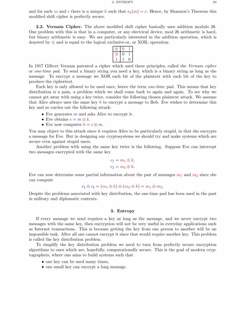
3. ENTROPY 83
and for each m and c there is a unique k such that ek(m) = c. Hence, by Shannon’s Theorem thismodified shift cipher is perfectly secure.
2.2. Vernam Cipher. The above modified shift cipher basically uses addition modulo 26.One problem with this is that in a computer, or any electrical device, mod 26 arithmetic is hard,but binary arithmetic is easy. We are particularly interested in the addition operation, which isdenoted by ⊕ and is equal to the logical exclusive-or, or XOR, operation:
⊕ 0 10 0 11 1 0
In 1917 Gilbert Vernam patented a cipher which used these principles, called the Vernam cipheror one-time pad. To send a binary string you need a key, which is a binary string as long as themessage. To encrypt a message we XOR each bit of the plaintext with each bit of the key toproduce the ciphertext.
Each key is only allowed to be used once, hence the term one-time pad. This means that keydistribution is a pain, a problem which we shall come back to again and again. To see why wecannot get away with using a key twice, consider the following chosen plaintext attack. We assumethat Alice always uses the same key k to encrypt a message to Bob. Eve wishes to determine thiskey and so carries out the following attack:
• Eve generates m and asks Alice to encrypt it.• Eve obtains c = m⊕ k.• Eve now computes k = c⊕m.
You may object to this attack since it requires Alice to be particularly stupid, in that she encryptsa message for Eve. But in designing our cryptosystems we should try and make systems which aresecure even against stupid users.
Another problem with using the same key twice is the following. Suppose Eve can intercepttwo messages encrypted with the same key
c1 = m1 ⊕ k,
c2 = m2 ⊕ k.
Eve can now determine some partial information about the pair of messages m1 and m2 since shecan compute
c1 ⊕ c2 = (m1 ⊕ k) ⊕ (m2 ⊕ k) = m1 ⊕m2.
Despite the problems associated with key distribution, the one-time pad has been used in the pastin military and diplomatic contexts.
3. Entropy
If every message we send requires a key as long as the message, and we never encrypt twomessages with the same key, then encryption will not be very useful in everyday applications suchas Internet transactions. This is because getting the key from one person to another will be animpossible task. After all one cannot encrypt it since that would require another key. This problemis called the key distribution problem.
To simplify the key distribution problem we need to turn from perfectly secure encryptionalgorithms to ones which are, hopefully, computationally secure. This is the goal of modern cryp-tographers, where one aims to build systems such that
• one key can be used many times,• one small key can encrypt a long message.
84 5. INFORMATION THEORETIC SECURITY
Such systems will not be unconditionally secure, by Shannon’s Theorem, and so must be at bestonly computationally secure.
We now need to develop the information theory needed to deal with these computationallysecure systems. Again the main results are due to Shannon in the late 1940s. In particular we shalluse Shannon’s idea of using entropy as a way of measuring information.
The word entropy is another name for uncertainty, and the basic tenet of information theoryis that uncertainty and information are essentially the same thing. This takes some getting usedto, but consider that if you are uncertain what something means then revealing the meaning givesyou information. As a cryptographic application suppose you want to determine the informationin a ciphertext, in other words you want to know what its true meaning is,
• you are uncertain what the ciphertext means,• you could guess the plaintext,• the level of uncertainty you have about the plaintext is the amount of information contained
in the ciphertext.If X is a random variable, the amount of entropy (in bits) associated with X is denoted by H(X),we shall define this quantity formally in a second. First let us look at a simple example to helpclarify ideas.
Suppose X is the answer to some question, i.e. Yes or No. If you know I will always say Yesthen my answer gives you no information. So the information contained in X should be zero, i.e.H(X) = 0. There is no uncertainty about what I will say, hence no information is given by mesaying it, hence there is no entropy.
If you have no idea what I will say and I reply Yes with equal probability to replying No thenI am revealing one bit of information. Hence, we should have H(X) = 1.
Note that entropy does not depend on the length of the actual message; in the above case wehave a message of length at most three letters but the amount of information is at most one bit.We can now define formally the notion of entropy.
Definition 5.5 (Entropy). Let X be a random variable which takes on a finite set of valuesxi, with 1 ≤ i ≤ n, and has probability distribution pi = p(X = xi). The entropy of X is defined tobe
H(X) = −n∑i=1
pi log2 pi.
We make the convention that if pi = 0 then pi log2 pi = 0.Let us return to our Yes or No question above and show that this definition of entropy coincides
with our intuition. Recall, X is the answer to some question with responses Yes or No. If youknow I will always say Yes then
p1 = 1 and p2 = 0.We compute
H(X) = −1 · log2 1 − 0 · log2 0 = 0.Hence, my answer reveals no information to you.
If you have no idea what I will say and I reply Yes with equal probability to replying No then
p1 = p2 = 1/2.
We now compute
H(X) = − log212
2− log2
12
2= 1.
Hence, my answer reveals one bit of information to you.
There are a number of elementary properties of entropy which follow from the definition.
3. ENTROPY 85
• We always have H(X) ≥ 0.• The only way to obtain H(X) = 0 is if for some i we have pi = 1 and pj = 0 when i �= j.• If pi = 1/n for all i then H(X) = log2 n.
Another way of looking at entropy is that it measures by how much one can compress the informa-tion. If I send a single ASCII character to signal Yes or No, for example I could simply send Y orN, I am actually sending 8 bits of data, but I am only sending one bit of information. If I wanted toI could compress the data down to 1/8th of its original size. Hence, naively if a message of lengthn can be compressed to a proportion ε of its original size then it contains ε · n bits of informationin it.
Let us return to our baby cryptosystem considered in the previous section. Recall we had theprobability spaces
P = {a, b, c, d}, K = {k1, k2, k3} and C = {1, 2, 3, 4},with the associated probabilities:
• p(P = a) = 0.25, p(P = b) = p(P = d) = 0.3 and p(P = c) = 0.15,• p(K = k1) = p(K = k3) = 0.25 and p(K = k2) = 0.5,• p(C = 1) = p(C = 2) = p(C = 3) = 0.2625 and p(C = 4) = 0.2125.
We can then calculate the relevant entropies as:
H(P ) ≈ 1.9527,
H(K) ≈ 1.5,
H(C) ≈ 1.9944.
Hence the ciphertext ‘leaks’ about two bits of information about the key and plaintext, since thatis how much information is contained in a single ciphertext. Later we will calculate how much ofthis information is about the key and how much about the plaintext.
We wish to derive an upper bound for the entropy of a random variable, to go with our lowerbound of H(X) ≥ 0. To do this we will need the following special case of Jensen’s inequality.
Theorem 5.6 (Jensen’s Inequality). Supposen∑i=1
ai = 1
with ai > 0 for 1 ≤ i ≤ n. Then, for xi > 0,n∑i=1
ai log2 xi ≤ log2
(n∑i=1
aixi
).
With equality occurring if and only if x1 = x2 = . . . = xn.
Using this we can now prove the following theorem:
Theorem 5.7. If X is a random variable which takes n possible values then
0 ≤ H(X) ≤ log2 n.
The lower bound is obtained if one value occurs with probability one, the upper bound is obtained ifall values are equally likely.
Proof. We have already discussed the facts about the lower bound so we will concentrateon the statements about the upper bound. The hypothesis is that X is a random variable with
86 5. INFORMATION THEORETIC SECURITY
probability distribution p1, . . . , pn, with pi > 0 for all i. One can then deduce the following sequenceof inequalities
H(X) = −n∑i=1
pi log2 pi
=n∑i=1
pi log2
1pi
≤ log2
(n∑i=1
(pi × 1
pi
))by Jensen’s inequality
= log2 n.
To obtain equality, we require equality when we apply Jensen’s inequality. But this will only occurwhen pi = 1/n for all i, in other words all values of X are equally likely. �
The basics of the theory of entropy closely match that of the theory of probability. For example,if X and Y are random variables then we define the joint probability distribution as
ri,j = p(X = xi and Y = yj)
for 1 ≤ i ≤ n and 1 ≤ j ≤ m.The joint entropy is then obviously defined as
H(X,Y ) = −n∑i=1
m∑j=1
ri,j log2 ri,j.
You should think of the joint entropy H(X,Y ) as the total amount of information contained in oneobservation of (x, y) ∈ X × Y . We then obtain the inequality
H(X,Y ) ≤ H(X) +H(Y )
with equality if and only if X and Y are independent. We leave the proof of this as an exercise.Just as with probability theory, where one has the linked concepts of joint probability and
conditional probability, so the concept of joint entropy is linked to the concept of conditionalentropy. This is important to understand, since conditional entropy is the main tool we shall usein understanding non-perfect ciphers in the rest of this chapter.
LetX and Y be two random variables. Recall we defined the conditional probability distributionas
p(X = x|Y = y) = Probability that X = x given Y = y.
The entropy of X given an observation of Y = y is then defined in the obvious way by
H(X|y) = −∑x
p(X = x|Y = y) log2 p(X = x|Y = y).
Given this we define the conditional entropy of X given Y as
H(X|Y ) =∑y
p(Y = y)H(X|y)
= −∑x
∑y
p(Y = y)p(X = x|Y = y) log2 p(X = x|Y = y).
This is the amount of uncertainty about X that is left after revealing a value of Y . The conditionaland joint entropy are linked by the following formula
H(X,Y ) = H(Y ) +H(X|Y )
3. ENTROPY 87
and we have the following upper bound
H(X|Y ) ≤ H(X)
with equality if and only if X and Y are independent. Again we leave the proof of these statementsas an exercise.
Now turning to cryptography again, we have some trivial statements relating the entropy of P ,K and C.
• H(P |K,C) = 0 :If you know the ciphertext and the key then you know the plaintext. This must hold sinceotherwise decryption will not work correctly.
• H(C|P,K) = 0 :If you know the plaintext and the key then you know the ciphertext. This holds for allciphers we have seen so far, and holds for all the symmetric ciphers we shall see in laterchapters. However, for modern public key encryption schemes we do not have this lastproperty when they are used correctly.
In addition we have the following identities
H(K,P,C) = H(P,K) +H(C|P,K) as H(X,Y ) = H(Y ) +H(X|Y )= H(P,K) as H(C|P,K) = 0= H(K) +H(P ) as K and P are independent
andH(K,P,C) = H(K,C) +H(P |K,C) as H(X,Y ) = H(Y ) +H(X|Y )
= H(K,C) as H(P |K,C) = 0.
Hence, we obtain
H(K,C) = H(K) +H(P ).
This last equality is important since it is related to the conditional entropy H(K|C), which is calledthe key equivocation. The key equivocation is the amount of uncertainty about the key left after oneciphertext is revealed. Recall that our goal is to determine the key given the ciphertext. Puttingtwo of our prior equalities together we find
(8) H(K|C) = H(K,C) −H(C) = H(K) +H(P ) −H(C).
In other words, the uncertainty about the key left after we reveal a ciphertext is equal to theuncertainty in the plaintext and the key minus the uncertainty in the ciphertext. Returning to ourprevious example, recall we had previously computed
H(P ) ≈ 1.9527,
H(K) ≈ 1.5,
H(C) ≈ 1.9944.
Hence
H(K|C) ≈ 1.9527 + 1.5 − 1.9944 ≈ 1.4583.
So around one and a half bits of information about the key are left to be found, on average, aftera single ciphertext is observed. This explains why the system leaks information, and shows that itcannot be secure. After all there are only 1.5 bits of uncertainty about the key to start with, oneciphertext leaves us with 1.4593 bits of uncertainty. Hence, 1.5−1.4593 = 0.042 bits of informationabout the key are revealed by a single ciphertext.
88 5. INFORMATION THEORETIC SECURITY
4. Spurious Keys and Unicity Distance
In our baby example above, information about the key is leaked by an individual ciphertext,since knowing the ciphertext rules out a certain subset of the keys. Of the remaining possible keys,only one is correct. The remaining possible, but incorrect, keys are called the spurious keys.
Consider the (unmodified) shift cipher, i.e. where the same key is used for each letter. Supposethe ciphertext is WNAJW, and suppose we know that the plaintext is an English word. The only‘meaningful’ plaintexts are RIVER and ARENA, which correspond to the two possible keys F andW . One of these keys is the correct one and one is spurious.
We can now explain why it was easy to break the substitution cipher in terms of a conceptcalled the unicity distance of the cipher. We shall explain this relationship in more detail, but wefirst need to understand the underlying plaintext in more detail. The plaintext in many computercommunications can be considered as a random bit string. But often this is not so. Sometimesone is encrypting an image or sometimes one is encrypting plain English text. In our discussion weshall consider the case when the underlying plaintext is taken from English, as in the substitutioncipher. Such a language is called a natural language to distinguish it from the bitstreams used bycomputers to communicate.
We first wish to define the entropy (or information) per letter HL of a natural language suchas English. Note, a random string of alphabetic characters would have entropy
log2 26 ≈ 4.70.
So we have HL ≤ 4.70. If we let P denote the random variable of letters in the English languagethen we have
p(P = a) = 0.082, . . . , p(P = e) = 0.127, . . . , p(P = z) = 0.001.
We can then computeHL ≤ H(P ) ≈ 4.14.
Hence, instead of 4.7 bits of information per letter, if we only examine the letter frequencies weconclude that English conveys around 4.14 bits of information per letter.
But this is a gross overestimate, since letters are not independent. For example Q is alwaysfollowed by U and the bigram TH is likely to be very common. One would suspect that a betterstatistic for the amount of entropy per letter could be obtained by looking at the distribution ofbigrams. Hence, we let P 2 denote the random variable of bigrams. If we let p(P = i, P ′ = j) denotethe random variable which is assigned the probability that the bigram ‘ij’ appears, then we define
H(P 2) = −∑i,j
p(P = i, P ′ = j) log p(P = i, P ′ = j).
A number of people have computed values of H(P 2) and it is commonly accepted to be given by
H(P 2) ≈ 7.12.
We want the entropy per letter so we compute
HL ≤ H(P 2)/2 ≈ 3.56.
But again this is an overestimate, since we have not taken into account that the most commontrigram is THE. Hence, we can also look at P 3 and compute H(P 3)/3. This will also be anoverestimate and so on...
This leads us to the following definition.
Definition 5.8. The entropy of the natural language L is defined to be
HL = limn−→∞
H(Pn)n
.
4. SPURIOUS KEYS AND UNICITY DISTANCE 89
The exact value of HL is hard to compute exactly but we can approximate it. In fact one has,by experiment, that for English
1.0 ≤ HL ≤ 1.5.
So each letter in English
• requires 5 bits of data to represent it,• only gives at most 1.5 bits of information.
This shows that English contains a high degree of redundancy. One can see this from the following,which you can still hopefully read (just) even though I have deleted two out of every four letters,
On** up** a t**e t**re **s a **rl **ll** Sn** Wh**e.
The redundancy of a language is defined by
RL = 1 − HL
log2 #P.
If we take HL ≈ 1.25 then the redundancy of English is
RL ≈ 1 − 1.25log2 26
= 0.75.
So this means that we should be able to compress an English text file of around 10 MB down to2.5 MB.
We now return to a general cipher and suppose c ∈ Cn, i.e. c is a ciphertext consisting of ncharacters. We define K(c) to be the set of keys which produce a ‘meaningful’ decryption of c.Then, clearly #K(c) − 1 is the number of spurious keys given c. The average number of spuriouskeys is defined to be sn, where
sn =∑c∈Cn
p(C = c) (#K(c) − 1)
=∑c∈Cn
p(C = c)#K(c) −∑c∈Cn
p(C = c)
=
(∑c∈Cn
p(C = c)#K(c)
)− 1.
90 5. INFORMATION THEORETIC SECURITY
Now if n is sufficiently large and #P = #C we obtain
log2(sn + 1) = log2
∑c∈Cn
p(C = c)#K(c)
≥∑c∈Cn
p(C = c) log2 #K(c) Jensen’s inequality
≥∑c∈Cn
p(C = c)H(K|c)
= H(K|Cn) By definition
= H(K) +H(Pn) −H(Cn) Equation (8)
≈ H(K) + nHL −H(Cn) If n is very large
= H(K) −H(Cn)
+ n(1 −RL) log2 #P By definition of RL≥ H(K) − n log2 #C
+ n(1 −RL) log2 #P As H(Cn) ≤ n log2 #C
= H(K) − nRL log2 #P As #P = #C.
So, if n is sufficiently large and #P = #C then
sn ≥ #K
#PnRL− 1.
As an attacker we would like the number of spurious keys to become zero, and it is clear that aswe take longer and longer ciphertexts then the number of spurious keys must go down.
The unicity distance n0 of a cipher is the value of n for which the expected number of spuriouskeys becomes zero. In other words this is the average amount of ciphertext needed before anattacker can determine the key, assuming the attacker has infinite computing power. For a perfectcipher we have n0 = ∞, but for other ciphers the value of n0 can be alarmingly small. We canobtain an estimate of n0 by setting sn = 0 in
sn ≥ #K
#PnRL− 1
to obtainn0 ≈ log2 #K
RL log2 #P.
In the substitution cipher we have
#P = 26,
#K = 26! ≈ 4 · 1026
and using our value of RL = 0.75 for English we can approximate the unicity distance as
n0 ≈ 88.40.75 × 4.7
≈ 25.
So we require on average only 25 ciphertext characters before we can break the substitution cipher,again assuming infinite computing power. In any case after 25 characters we expect a unique validdecryption.
Now assume we have a modern cipher which encrypts bit strings using keys of bit length l, wehave
#P = 2,
#K = 2l.
Further Reading 91
Again we assume RL = 0.75, which is an underestimate since we now need to encode English intoa computer communications media such as ASCII. Then the unicity distance is
n0 ≈ l
0.75=
4l3.
Now assume instead of transmitting the plain ASCII we compress it first. If we assume a perfectcompression algorithm then the plaintext will have no redundancy and so RL ≈ 0. In which casethe unicity distance is
n0 ≈ l
0= ∞.
So you may ask if modern ciphers encrypt plaintexts with no redundancy? The answer is no,even if one compresses the data, a modern cipher often adds some redundancy to the plaintextbefore encryption. The reason is that we have only considered passive attacks, i.e. an attackerhas been only allowed to examine ciphertexts and from these ciphertexts the attacker’s goal is todetermine the key. There are other types of attack called active attacks, in these an attacker isallowed to generate plaintexts or ciphertexts of her choosing and ask the key holder to encryptor decrypt them, the two variants being called a chosen plaintext attack and a chosen ciphertextattack respectively.
In public key systems that we shall see later, chosen plaintexts attacks cannot be stopped sinceanyone is allowed to encrypt anything. We would however, like to stop chosen ciphertext attacks.The current wisdom for public key algorithms is to make the cipher add some redundancy to theplaintext before it is encrypted. In that way it is hard for an attacker to produce a ciphertext whichhas a valid decryption. The philosophy is that it is then hard for an attacker to mount a chosenciphertext attack, since it will be hard for an attacker to choose a valid ciphertext for a decryptionquery. We shall discuss this more in later chapters.
Chapter Summary
• A cryptographic system for which knowing the ciphertext reveals no more informationthan if you did not know the ciphertext is called a perfectly secure system.
• Perfectly secure systems exist, but they require keys as long as the message and a differentkey to be used with each new encryption. Hence, perfectly secure systems are not verypractical.
• Information and uncertainty are essentially the same thing. An attacker really wants,given the ciphertext, to determine some information about the plaintext. The amount ofuncertainty in a random variable is measured by its entropy.
• The equation H(K|C) = H(K)+H(P )−H(C) allows us to estimate how much uncertaintyremains about the key after one observes a single ciphertext.
• The natural redundancy of English means that a naive cipher does not need to produce alot of ciphertext before the underlying plaintext can be discovered.
Further Reading
Our discussion of Shannon’s theory has closely followed the treatment in the book by Stinson.Another possible source of information is the book by Welsh. A general introduction to informationtheory, including its application to coding theory is in the book by van der Lubbe.
92 5. INFORMATION THEORETIC SECURITY
J.C.A. van der Lubbe. Information Theory. Cambridge University Press, 1997.
D. Stinson. Cryptography: Theory and Practice. CRC Press, 1995.
D. Welsh. Codes and Cryptography. Oxford University Press, 1988.
CHAPTER 6
Historical Stream Ciphers
Chapter Goals
• To introduce the general model for symmetric ciphers.• To explain the relation between stream ciphers and the Vernam cipher.• To examine the working and breaking of the Lorenz cipher in detail.
1. Introduction To Symmetric Ciphers
A symmetric cipher works using the following two transformations
c = ek(m),
m = dk(c)
where• m is the plaintext,• e is the encryption function,• d is the decryption function,• k is the secret key,• c is the ciphertext.
It should be noted that it is desirable that both the encryption and decryption functions are publicknowledge and that the secrecy of the message, given the ciphertext, depends totally on the secrecyof the secret key, k. Although this well-established principle, called Kerckhoffs’ principle, hasbeen known since the mid-1800s many companies still ignore it. There are instances of companiesdeploying secret proprietary encryption schemes which turn out to be insecure as soon as someoneleaks the details of the algorithms. The best schemes will be the ones which have been studied bya lot of people for a very long time and which have been found to remain secure. A scheme whichis a commercial secret cannot be studied by anyone outside the company.
The above setup is called a symmetric key system since both parties need access to the secretkey. Sometimes symmetric key cryptography is implemented using two keys, one for encryptionand one for decryption. However, if this is the case we assume that given the encryption key it iseasy to compute the decryption key (and vice versa). Later we shall meet public key cryptographywhere only one key is kept secret, called the private key, the other key, called the public key isallowed to be published in the clear. In this situation it is assumed to be computationally infeasiblefor someone to compute the private key given the public key.
Returning to symmetric cryptography, a moment’s thought reveals that the number of possiblekeys must be very large. This is because in designing a cipher we assume the worst case scenarioand give the attacker the benefit of
• full knowledge of the encryption/decryption algorithm,• a number of plaintext/ciphertext pairs associated to the target key k.
93
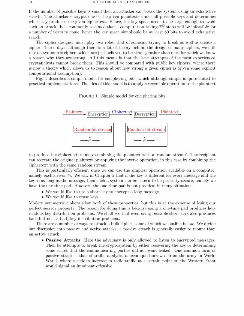
94 6. HISTORICAL STREAM CIPHERS
If the number of possible keys is small then an attacker can break the system using an exhaustivesearch. The attacker encrypts one of the given plaintexts under all possible keys and determineswhich key produces the given ciphertext. Hence, the key space needs to be large enough to avoidsuch an attack. It is commonly assumed that a computation taking 280 steps will be infeasible fora number of years to come, hence the key space size should be at least 80 bits to avoid exhaustivesearch.
The cipher designer must play two roles, that of someone trying to break as well as create acipher. These days, although there is a lot of theory behind the design of many ciphers, we stillrely on symmetric ciphers which are just believed to be strong, rather than ones for which we knowa reason why they are strong. All this means is that the best attempts of the most experiencedcryptanalysts cannot break them. This should be compared with public key ciphers, where thereis now a theory which allows us to reason about how strong a given cipher is (given some explicitcomputational assumption).
Fig. 1 describes a simple model for enciphering bits, which although simple is quite suited topractical implementations. The idea of this model is to apply a reversible operation to the plaintext
Figure 1. Simple model for enciphering bits
Plaintext Encryption Ciphertext Decryption Plaintext
Random bit stream
⊕
Random bit stream
⊕
to produce the ciphertext, namely combining the plaintext with a ‘random stream’. The recipientcan recreate the original plaintext by applying the inverse operation, in this case by combining theciphertext with the same random stream.
This is particularly efficient since we can use the simplest operation available on a computer,namely exclusive-or ⊕. We saw in Chapter 5 that if the key is different for every message and thekey is as long as the message, then such a system can be shown to be perfectly secure, namely wehave the one-time pad. However, the one-time pad is not practical in many situations.
• We would like to use a short key to encrypt a long message.• We would like to reuse keys.
Modern symmetric ciphers allow both of these properties, but this is at the expense of losing ourperfect secrecy property. The reason for doing this is because using a one-time pad produces hor-rendous key distribution problems. We shall see that even using reusable short keys also producesbad (but not as bad) key distribution problems.
There are a number of ways to attack a bulk cipher, some of which we outline below. We divideour discussion into passive and active attacks; a passive attack is generally easier to mount thanan active attack.
• Passive Attacks: Here the adversary is only allowed to listen to encrypted messages.Then he attempts to break the cryptosystem by either recovering the key or determiningsome secret that the communicating parties did not want leaked. One common form ofpassive attack is that of traffic analysis, a technique borrowed from the army in WorldWar I, where a sudden increase in radio traffic at a certain point on the Western Frontwould signal an imminent offensive.
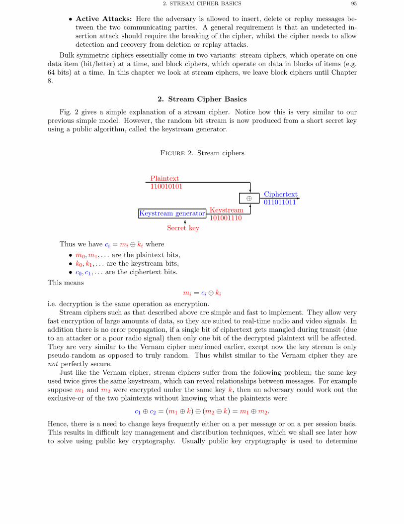
2. STREAM CIPHER BASICS 95
• Active Attacks: Here the adversary is allowed to insert, delete or replay messages be-tween the two communicating parties. A general requirement is that an undetected in-sertion attack should require the breaking of the cipher, whilst the cipher needs to allowdetection and recovery from deletion or replay attacks.
Bulk symmetric ciphers essentially come in two variants: stream ciphers, which operate on onedata item (bit/letter) at a time, and block ciphers, which operate on data in blocks of items (e.g.64 bits) at a time. In this chapter we look at stream ciphers, we leave block ciphers until Chapter8.
2. Stream Cipher Basics
Fig. 2 gives a simple explanation of a stream cipher. Notice how this is very similar to ourprevious simple model. However, the random bit stream is now produced from a short secret keyusing a public algorithm, called the keystream generator.
Figure 2. Stream ciphers
Secret key
Keystream generator
�
Keystream101001110
�
⊕ Ciphertext011011011
Plaintext110010101
Thus we have ci = mi ⊕ ki where• m0,m1, . . . are the plaintext bits,• k0, k1, . . . are the keystream bits,• c0, c1, . . . are the ciphertext bits.
This meansmi = ci ⊕ ki
i.e. decryption is the same operation as encryption.Stream ciphers such as that described above are simple and fast to implement. They allow very
fast encryption of large amounts of data, so they are suited to real-time audio and video signals. Inaddition there is no error propagation, if a single bit of ciphertext gets mangled during transit (dueto an attacker or a poor radio signal) then only one bit of the decrypted plaintext will be affected.They are very similar to the Vernam cipher mentioned earlier, except now the key stream is onlypseudo-random as opposed to truly random. Thus whilst similar to the Vernam cipher they arenot perfectly secure.
Just like the Vernam cipher, stream ciphers suffer from the following problem; the same keyused twice gives the same keystream, which can reveal relationships between messages. For examplesuppose m1 and m2 were encrypted under the same key k, then an adversary could work out theexclusive-or of the two plaintexts without knowing what the plaintexts were
c1 ⊕ c2 = (m1 ⊕ k) ⊕ (m2 ⊕ k) = m1 ⊕m2.
Hence, there is a need to change keys frequently either on a per message or on a per session basis.This results in difficult key management and distribution techniques, which we shall see later howto solve using public key cryptography. Usually public key cryptography is used to determine
96 6. HISTORICAL STREAM CIPHERS
session or message keys, and then the actual data is rapidly encrypted using either a stream orblock cipher.
The keystream generator above needs to produce a keystream with a number of properties forthe stream cipher to be considered secure. As a bare minimum the keystream should
• Have a long period. Since the keystream ki is produced via a deterministic process fromthe key, there will exist a number N such that
ki = ki+N
for all values of i. This number N is called the period of the sequence, and should be largefor the keystream generator to be considered secure.
• Have pseudo-random properties. The generator should produce a sequence which appearsto be random, in other words it should pass a number of statistical random number tests.
• Have large linear complexity. See Chapter 7 for what this means.However, these conditions are not sufficient. Generally determining more of the sequence from apart should be computationally infeasible. Ideally, even if one knows the first one billion bits ofthe keystream sequence, the probability of guessing the next bit correctly should be no better thanone half.
In Chapter 7 we shall discuss how stream ciphers are created using a combination of simplecircuits called Linear Feedback Shift Registers. But first we will look at earlier constructions usingrotor machines, or in modern notation Shift Registers (i.e. shift registers with no linear feedback).
3. The Lorenz Cipher
The Lorenz cipher was a German cipher from World War Two which was used for strategicinformation, as opposed to the tactical and battlefield information encrypted under the Enigmamachine. The Lorenz machine was a stream cipher which worked on streams of bits. However itdid not produce a single stream of bits, it produced five. The reason was due to the encoding ofteleprinter messages used at the time, namely Baudot code.
3.1. Baudot Code. To understand the Lorenz cipher we first need to understand Baudotcode. We all are aware of the ASCII encoding for the standard letters on a keyboard, this usesseven bits for the data, plus one bit for error detection. Prior to ASCII, indeed as far back as 1870,Baudot invented an encoding which used five bits of data. This was further developed until, by the1930’s, it was the standard method of communicating via teleprinter. The data was encoding viaa tape, which consisted of a sequence of five rows of holes/non-holes.
Those of us of a certain age in the United Kingdom can remember the football scores beingsent in on a Saturday evening by teleprinter, and those who are even older can maybe recall theticker-tape parades in New York. The ticker-tape was the remains of transmitted messages inBaudot code. For those who can remember early dial-up modems, they will recall that the speedswere measured in Baud’s, or characters per second, in memory of Baudot’s invention.
Now five bits does not allow one to encode all the characters that one wants, thus Baudot codeused two possible “states” called letters shift and figures shift. Moving between the two states wascontrolled by control characters, a number of other control characters were reserved for things suchas space (SP), carriage return (CR), line feed (LF) or a character which rung the teleprinters bell(BELL) (such a code still exists in ASCII). The table for Baudot code in the 1930’s is presented inTable 1.
Thus to transmit the messagePlease, Please Help!
one would need to transmit the encoding, which we give in hexadecimal,16, 12, 01, 03, 05, 01, 1B, 0C, 1F, 04, 16, 12, 01, 03, 05, 01, 04, 14, 01, 12, 16, 1B, 0D.
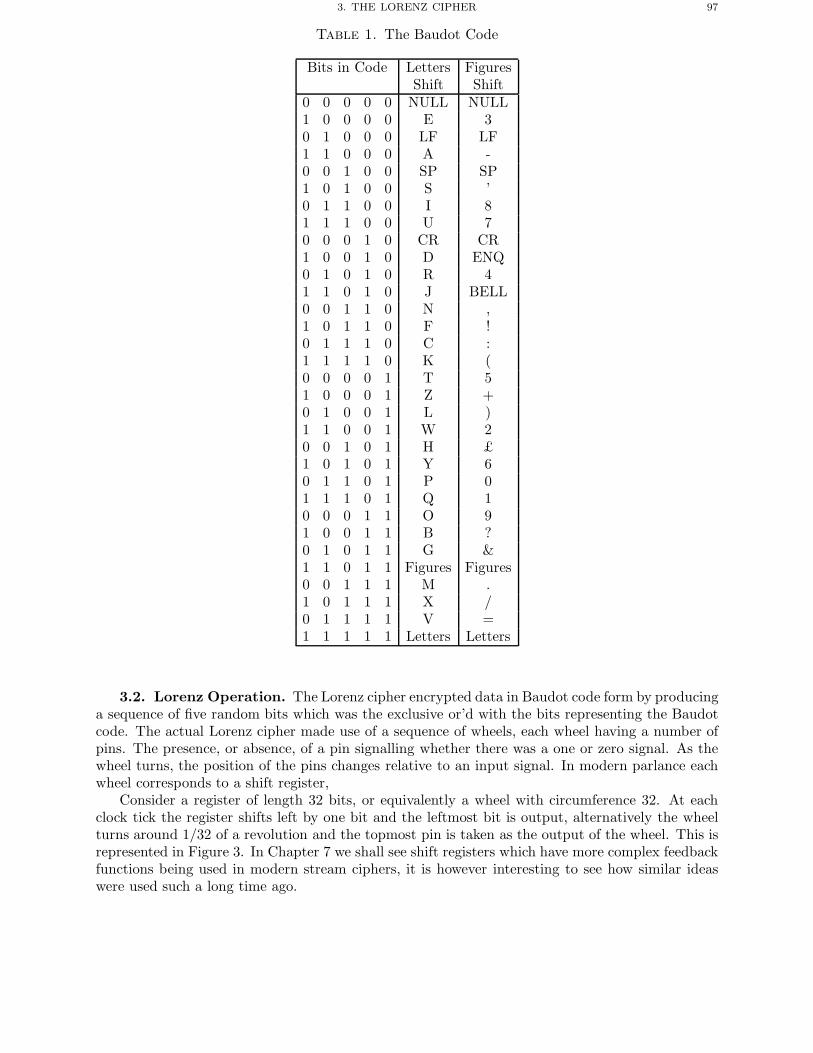
3. THE LORENZ CIPHER 97
Table 1. The Baudot Code
Bits in Code Letters FiguresShift Shift
0 0 0 0 0 NULL NULL1 0 0 0 0 E 30 1 0 0 0 LF LF1 1 0 0 0 A -0 0 1 0 0 SP SP1 0 1 0 0 S ’0 1 1 0 0 I 81 1 1 0 0 U 70 0 0 1 0 CR CR1 0 0 1 0 D ENQ0 1 0 1 0 R 41 1 0 1 0 J BELL0 0 1 1 0 N ,1 0 1 1 0 F !0 1 1 1 0 C :1 1 1 1 0 K (0 0 0 0 1 T 51 0 0 0 1 Z +0 1 0 0 1 L )1 1 0 0 1 W 20 0 1 0 1 H £1 0 1 0 1 Y 60 1 1 0 1 P 01 1 1 0 1 Q 10 0 0 1 1 O 91 0 0 1 1 B ?0 1 0 1 1 G &1 1 0 1 1 Figures Figures0 0 1 1 1 M .1 0 1 1 1 X /0 1 1 1 1 V =1 1 1 1 1 Letters Letters
3.2. Lorenz Operation. The Lorenz cipher encrypted data in Baudot code form by producinga sequence of five random bits which was the exclusive or’d with the bits representing the Baudotcode. The actual Lorenz cipher made use of a sequence of wheels, each wheel having a number ofpins. The presence, or absence, of a pin signalling whether there was a one or zero signal. As thewheel turns, the position of the pins changes relative to an input signal. In modern parlance eachwheel corresponds to a shift register,
Consider a register of length 32 bits, or equivalently a wheel with circumference 32. At eachclock tick the register shifts left by one bit and the leftmost bit is output, alternatively the wheelturns around 1/32 of a revolution and the topmost pin is taken as the output of the wheel. This isrepresented in Figure 3. In Chapter 7 we shall see shift registers which have more complex feedbackfunctions being used in modern stream ciphers, it is however interesting to see how similar ideaswere used such a long time ago.
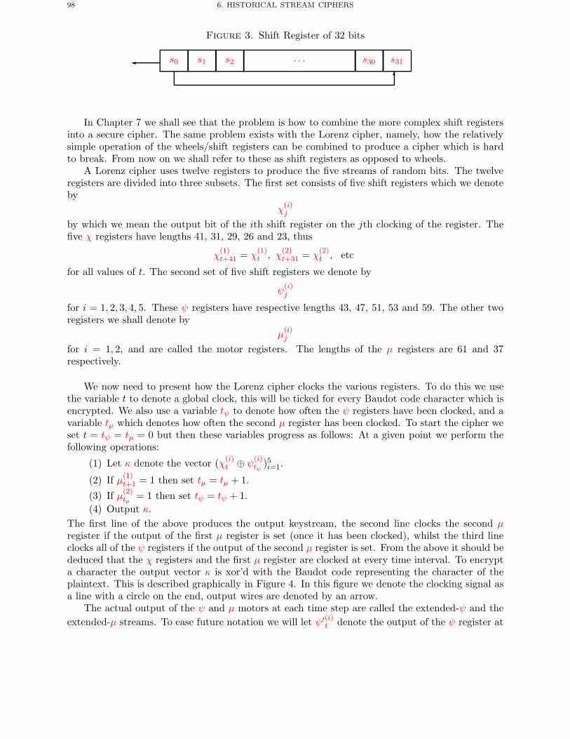
98 6. HISTORICAL STREAM CIPHERS
Figure 3. Shift Register of 32 bits
� s0 s1 s2 . . . s30 s31
�
In Chapter 7 we shall see that the problem is how to combine the more complex shift registersinto a secure cipher. The same problem exists with the Lorenz cipher, namely, how the relativelysimple operation of the wheels/shift registers can be combined to produce a cipher which is hardto break. From now on we shall refer to these as shift registers as opposed to wheels.
A Lorenz cipher uses twelve registers to produce the five streams of random bits. The twelveregisters are divided into three subsets. The first set consists of five shift registers which we denoteby
χ(i)j
by which we mean the output bit of the ith shift register on the jth clocking of the register. Thefive χ registers have lengths 41, 31, 29, 26 and 23, thus
χ(1)t+41 = χ
(1)t , χ
(2)t+31 = χ
(2)t , etc
for all values of t. The second set of five shift registers we denote by
ψ(i)j
for i = 1, 2, 3, 4, 5. These ψ registers have respective lengths 43, 47, 51, 53 and 59. The other tworegisters we shall denote by
μ(i)j
for i = 1, 2, and are called the motor registers. The lengths of the μ registers are 61 and 37respectively.
We now need to present how the Lorenz cipher clocks the various registers. To do this we usethe variable t to denote a global clock, this will be ticked for every Baudot code character which isencrypted. We also use a variable tψ to denote how often the ψ registers have been clocked, and avariable tμ which denotes how often the second μ register has been clocked. To start the cipher weset t = tψ = tμ = 0 but then these variables progress as follows: At a given point we perform thefollowing operations:
(1) Let κ denote the vector (χ(i)t ⊕ ψ
(i)tψ
)5i=1.
(2) If μ(1)t+1 = 1 then set tμ = tμ + 1.
(3) If μ(2)tμ = 1 then set tψ = tψ + 1.
(4) Output κ.The first line of the above produces the output keystream, the second line clocks the second μregister if the output of the first μ register is set (once it has been clocked), whilst the third lineclocks all of the ψ registers if the output of the second μ register is set. From the above it should bededuced that the χ registers and the first μ register are clocked at every time interval. To encrypta character the output vector κ is xor’d with the Baudot code representing the character of theplaintext. This is described graphically in Figure 4. In this figure we denote the clocking signal asa line with a circle on the end, output wires are denoted by an arrow.
The actual output of the ψ and μ motors at each time step are called the extended-ψ and theextended-μ streams. To ease future notation we will let ψ′(i)
t denote the output of the ψ register at
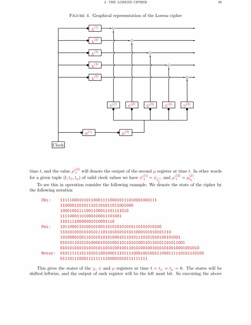
3. THE LORENZ CIPHER 99
Figure 4. Graphical representation of the Lorenz cipher
Clock
� μ(1) � μ(2)
� χ(1)
� χ(2)
� χ(3)
� χ(4)
� χ(5)
�ψ(1)
�ψ(2)
�ψ(3)
�ψ(4)
�ψ(5)
⊕
.................................
.................................
.................................
.................................
�⊕
.................................
.................................
.................................
�⊕
.................................
.................................
�⊕
.................................
�
�⊕
time t, and the value μ′(2)t will denote the output of the second μ register at time t. In other wordsfor a given tuple (t, tψ, tμ) of valid clock values we have ψ′(i)
t = ψt(i)ψ
and μ′(2)t = μ(2)tμ .
To see this in operation consider the following example: We denote the state of the cipher bythe following notation
Chi: 111110001010110001111000101110100010001111100001101011101101011011001000100010011110011000111011110101111000110100010001110100111011110000001010001110
Psi: 1011000110100101001101010101010110101010100110101010101010111011010101010110001010101011101010000100110101010101000101101011101010101001010010101011010101000010101001101101010011011010110101100101010101010101010110101001001101010010010101010010001001010
Motor: 01011111101101011001000111011110001001001110001111101011101000111011100011111111100001010111111111
This gives the states of the χ, ψ and μ registers at time t = tψ = tμ = 0. The states will beshifted leftwise, and the output of each register will be the left most bit. So executing the above
100 6. HISTORICAL STREAM CIPHERS
algorithm at time t = 0 the output first key vector will be
κ0 = χ0 ⊕ ψ0 =
⎛⎜⎜⎜⎜⎝
11111
⎞⎟⎟⎟⎟⎠⊕
⎛⎜⎜⎜⎜⎝
11100
⎞⎟⎟⎟⎟⎠ =
⎛⎜⎜⎜⎜⎝
00011
⎞⎟⎟⎟⎟⎠ .
Then since μ(1)1 = 1 we clock the tμ value, and then since μ(2)
1 = 1 we also clock the tψ value. Thusat time t = 1 the state of the Lorenz cipher becomes
Chi: 111100010101100011110001011101000100011111000011010111011010110110010001000100111100110001110111101011110001101000100011101001110111100000010100011101
Psi: 0110001101001010011010101010101101010101001101010101010101110110101010101100010101010111010100001001101010101010001011010111010101010010100111010110101010000101010011011010100110110101101011001010101010101010101101010010011010100100101010100100010010100
Motor: 10111111011010110010001110111100010010011100011111010111010001110111000111111111000010101111111110
Now we look at what happens at the next clock tick. At time t = 1 we now output the vector
κ1 = χ1 ⊕ ψ0 =
⎛⎜⎜⎜⎜⎝
11011
⎞⎟⎟⎟⎟⎠⊕
⎛⎜⎜⎜⎜⎝
01011
⎞⎟⎟⎟⎟⎠ =
⎛⎜⎜⎜⎜⎝
10000
⎞⎟⎟⎟⎟⎠ .
But now since μ(1)t+1 is equal to zero we do not clock tμ, which means that since μ(2)
1 = 1 we stillclock the tψ value. This process is then repeated, so that we obtain the following sequence for thefirst 60 output values of the keystream κt,
010010000101001011101100011011011101110001111111000000001001000100011101110011111010111110011000011011000111111101110111001010010110011011101110100001000100111100110010101101010000101000101101110010011011001011000110100011110001111101010111100011001000010001001000000101000000101000111000010011010011
This is produced by xor’ing the output of the χ registers, which is given by111110001010110001111000101110100010001111111100010101100011110000110101110110101101100100011000011010111011010110110010100010011110011000111011110101000100111100110001110111101010111100011010001000111010011111000110100010001110100111110001110111100000010100011101101111000000101000111011011110000001
by the values of output of the ψ′t stream at time t,
101100001111111010010100110101111111111110000011010101101010110100101000000101010111011010000000000001111100101011000101101000001000000011010101010100000000000000000011011010111010010100110111111010100001010100000000000001111111011010100110010100101000000101010101101010000000000000000011001101010010
3. THE LORENZ CIPHER 101
To ease understanding we also present the output μ′(2)t which is11110111100000111111111111111000000000001000010111111111111
Recall, a one in this stream means that the ψ registers are clocked whilst a zero implies they arenot clocked. One can see this effect in the ψ′
t output given earlier.
Just like the Enigma machine the Lorenz cipher has a long term key setup and a short termper message setup. The long term is the state of each register. Thus it appears there are a total of
241+31+29+26+23+43+47+51+53+59+61+37 = 2501
states, although the actual number is slightly less than this due to a small constraint which we beintroduced in a moment. In the early stages of the war the μ registers were changes on a daily basis,the χ registers were changed on a monthly basis and the ψ registers were changed on a monthly orquarterly basis. Thus, if the months settings had been broken, then the “day” key, “only” consistedof at most
261+37 = 298
states. As the war progressed the Germans moved to changing all the internal states of the registersevery day.
Then, given these “day” values for the register contents, the per message setting is given bythe starting position of each register. Thus the total number of message keys, given a day key, isgiven by
41 · 31 · 29 · 26 · 23 · 43 · 47 · 51 · 53 · 59 · 61 · 37 ≈ 264.
The Lorenz cipher has an obvious weakness as defined, which is what eventually led to itsbreaking, and which the Germans were aware of. The basic technique which we will use throughoutthe rest of this chapter is to take the ‘Delta’ of a sequence, this is defined as follows, for a sequences = (si)∞i=0,
Δs = (si ⊕ si+1)∞i=0.
We shall denote the value of the Δs sequence at time t by (Δs)t. The reason why the Δ operatoris so important in the analysis of the Lorenz cipher is due to the following observation: Since
κt = χt ⊕ ψtψ
andκt+1 = χt+1 ⊕
(μ′(2)t · ψtψ+1
)⊕((μ′(2)t − 1) · ψtψ
),
thus
(Δκ)t = (χt ⊕ χt+1) ⊕(μ′(2)t · (ψtψ ⊕ ψtψ+1
))= (Δχ)t ⊕
(μ′(2)t · (Δψ)tψ
).
Now if Pr[μ′(2)t = 1] = Pr[(Δψ)tψ = 1] = 1/2, as we would have by choosing the register statesuniformly at random, then with probability 3/4 the value of the Δκ stream reveals the value ofthe Δχ stream, which would enable the adversary to recover the state of the χ registers relativelyeasily. Thus the Germans imposed a restriction on the key values so that
Pr[μ′(2)t = 1] · Pr[(Δψ)tψ = 1] ≈ 1/2.
In what follows we shall denote these two probabilities by δ = Pr[μ′(2)t = 1] and ε = Pr[(Δψ)tψ = 1].Finally, to fix notation, if we let the Baudot encoding of the message be given by the sequence
φ of 5-bit vectors, and the ciphertext be given by the sequence γ then we have
γ(i)t = φ
(i)t ⊕ κ
(i)t .
102 6. HISTORICAL STREAM CIPHERS
As the war progressed more complex internal operations of the Lorenz cipher were introduced.These were called “limitations” by Bletchley, and they introduced extra complications into theclocking of the various registers. We shall ignore these extra complications however in our discus-sion.
Initially the Allies did not know anything about the Lorenz cipher, even that it consisted oftwelve wheels, let alone their period. In August 1941 the Germans made a serious mistake theytransmitted virtually identical 4000 character messages using the exactly the same key. From thisthe cryptanalyst J. Tiltman managed to reconstruct the 4000 character key that had been outputby the Lorenz cipher. From this sequence of 4000 apparently random strings of five bits anothercryptographer W.T. Tutte recovered the precise internal workings of the Lorenz cipher. The finalconfirmation that the internal workings had been deduced correctly did not come until the end ofthe war, when the allies obtained a Lorenz machine on entering Germany.
3.3. Breaking the Wheels. Having determined the structure of the Lorenz cipher the prob-lem remains on how to break it. The attack method were broken into two stages. In the first stagethe wheel’s needed to be broken, this was an involved process which only had to be performed oncefor each wheel configuration. Then a simpler procedure was produced which recovered the wheelpositions for each message.
We now explain how wheel breaking occurred. The first task is to obtain with reasonablecertainty the value of the sequence
Δκ(i) ⊕ Δκ(j)
for different distinct values of i and j, usually i = 1 and j = 2. There were various differentways of performing this, below we present a gross simplification of the techniques used by thecryptanalysts at Bletchley. Our goal is simply to show that breaking even a 60 year old streamcipher requires some intricate manipulation of probability estimates, and that even small deviationsfrom randomness in the output stream can cause a catastrophic failure in security.
To do this we first need to consider some characteristics of the plain text. Standard naturallanguage contains a larger sequence of repeated characters than one would normally expect, com-pared to the case when a message was just random gibberish. If messages where random then onewould expect
Pr[(Δφ(i))t ⊕ (Δφ(j))t = 0] = 1/2.
However, if the plaintext sequence contains slightly more repeated characters then we expect thisprobability to be slightly more than 1/2, so we set
(9) Pr[(Δφ(i))t ⊕ (Δφ(j))t = 0] = 1/2 + ρ.
Due to the nature of military German, and the Baudot encoding method, this was apparentlyparticularly pronounced when one considered the first and second stream of bits, i.e. i = 1 andj = 2.
There are essentially two situations for wheel breaking, the first (more complex) case is whenwe do not know the underlying plaintext for a message, i.e. the attacker only has access to theciphertext. The second case is when the attacker can guess with reasonable certainty the valueof the underlying plaintext (a “crib” in the Bletchley jargon), and so can obtain the resultingkeystream.
Ciphertext Only Method: The basic idea is that the sequence of ciphertext Delta’s,
Δγ(i) ⊕ Δγ(j)
will “reveal” the true value of the sequence
Δχ(i) ⊕ Δχ(j).
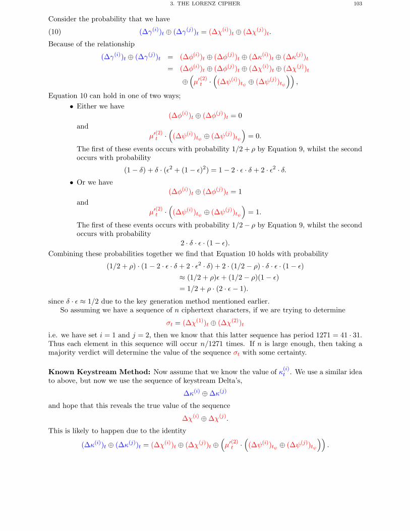
3. THE LORENZ CIPHER 103
Consider the probability that we have
(10) (Δγ(i))t ⊕ (Δγ(j))t = (Δχ(i))t ⊕ (Δχ(j))t.
Because of the relationship
(Δγ(i))t ⊕ (Δγ(j))t = (Δφ(i))t ⊕ (Δφ(j))t ⊕ (Δκ(i))t ⊕ (Δκ(j))t= (Δφ(i))t ⊕ (Δφ(j))t ⊕ (Δχ(i))t ⊕ (Δχ(j))t
⊕(μ′(2)t ·
((Δψ(i))tψ ⊕ (Δψ(j))tψ
)),
Equation 10 can hold in one of two ways;• Either we have
(Δφ(i))t ⊕ (Δφ(j))t = 0and
μ′(2)t ·((Δψ(i))tψ ⊕ (Δψ(j))tψ
)= 0.
The first of these events occurs with probability 1/2 + ρ by Equation 9, whilst the secondoccurs with probability
(1 − δ) + δ · (ε2 + (1 − ε)2) = 1 − 2 · ε · δ + 2 · ε2 · δ.• Or we have
(Δφ(i))t ⊕ (Δφ(j))t = 1and
μ′(2)t ·((Δψ(i))tψ ⊕ (Δψ(j))tψ
)= 1.
The first of these events occurs with probability 1/2− ρ by Equation 9, whilst the secondoccurs with probability
2 · δ · ε · (1 − ε).Combining these probabilities together we find that Equation 10 holds with probability
(1/2 + ρ) · (1 − 2 · ε · δ + 2 · ε2 · δ) + 2 · (1/2 − ρ) · δ · ε · (1 − ε)
≈ (1/2 + ρ)ε+ (1/2 − ρ)(1 − ε)
= 1/2 + ρ · (2 · ε− 1).
since δ · ε ≈ 1/2 due to the key generation method mentioned earlier.So assuming we have a sequence of n ciphertext characters, if we are trying to determine
σt = (Δχ(1))t ⊕ (Δχ(2))t
i.e. we have set i = 1 and j = 2, then we know that this latter sequence has period 1271 = 41 · 31.Thus each element in this sequence will occur n/1271 times. If n is large enough, then taking amajority verdict will determine the value of the sequence σt with some certainty.
Known Keystream Method: Now assume that we know the value of κ(i)t . We use a similar idea
to above, but now we use the sequence of keystream Delta’s,
Δκ(i) ⊕ Δκ(j)
and hope that this reveals the true value of the sequence
Δχ(i) ⊕ Δχ(j).
This is likely to happen due to the identity
(Δκ(i))t ⊕ (Δκ(j))t = (Δχ(i))t ⊕ (Δχ(j))t ⊕(μ′(2)t ·
((Δψ(i))tψ ⊕ (Δψ(j))tψ
)).
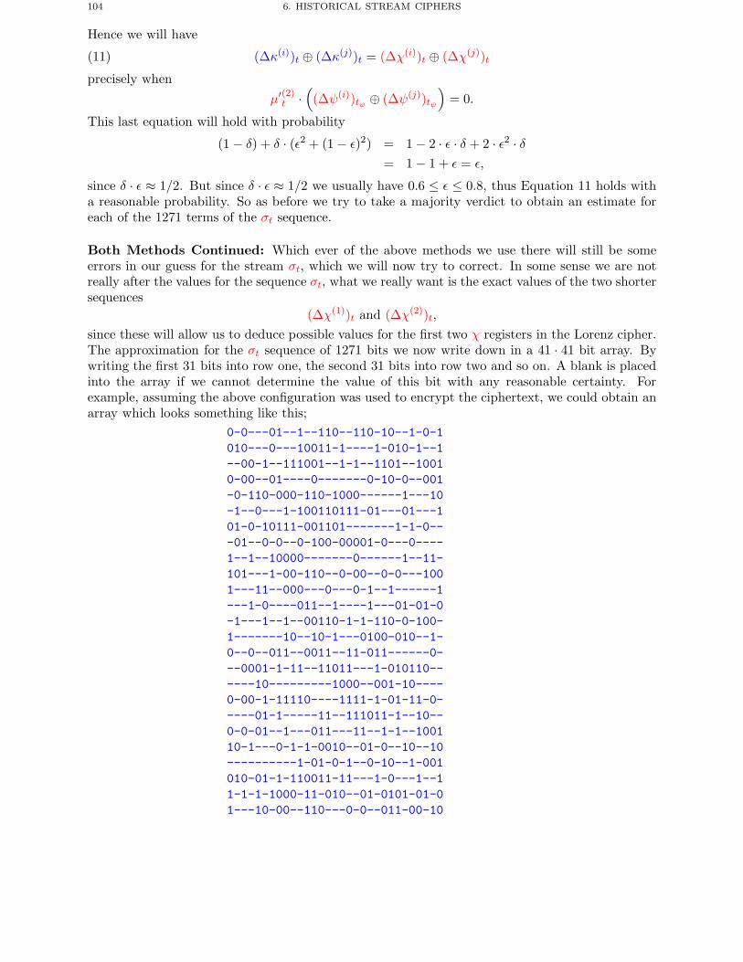
104 6. HISTORICAL STREAM CIPHERS
Hence we will have
(11) (Δκ(i))t ⊕ (Δκ(j))t = (Δχ(i))t ⊕ (Δχ(j))t
precisely whenμ′(2)t ·
((Δψ(i))tψ ⊕ (Δψ(j))tψ
)= 0.
This last equation will hold with probability
(1 − δ) + δ · (ε2 + (1 − ε)2) = 1 − 2 · ε · δ + 2 · ε2 · δ= 1 − 1 + ε = ε,
since δ · ε ≈ 1/2. But since δ · ε ≈ 1/2 we usually have 0.6 ≤ ε ≤ 0.8, thus Equation 11 holds witha reasonable probability. So as before we try to take a majority verdict to obtain an estimate foreach of the 1271 terms of the σt sequence.
Both Methods Continued: Which ever of the above methods we use there will still be someerrors in our guess for the stream σt, which we will now try to correct. In some sense we are notreally after the values for the sequence σt, what we really want is the exact values of the two shortersequences
(Δχ(1))t and (Δχ(2))t,since these will allow us to deduce possible values for the first two χ registers in the Lorenz cipher.The approximation for the σt sequence of 1271 bits we now write down in a 41 · 41 bit array. Bywriting the first 31 bits into row one, the second 31 bits into row two and so on. A blank is placedinto the array if we cannot determine the value of this bit with any reasonable certainty. Forexample, assuming the above configuration was used to encrypt the ciphertext, we could obtain anarray which looks something like this;
0-0---01--1--110--110-10--1-0-1010---0---10011-1----1-010-1--1--00-1--111001--1-1--1101--10010-00--01----0-------0-10-0--001-0-110-000-110-1000------1---10-1--0---1-100110111-01---01---101-0-10111-001101-------1-1-0---01--0-0--0-100-00001-0---0----1--1--10000-------0------1--11-101---1-00-110--0-00--0-0---1001---11--000---0---0-1--1------1---1-0----011--1----1---01-01-0-1---1--1--00110-1-1-110-0-100-1-------10--10-1---0100-010--1-0--0--011--0011--11-011------0---0001-1-11--11011---1-010110------10---------1000--001-10----0-00-1-11110----1111-1-01-11-0-----01-1-----11--111011-1--10--0-0-01--1---011---11--1-1--100110-1---0-1-1-0010--01-0--10--10----------1-01-0-1--0-10--1-001010-01-1-110011-11---1-0---1--11-1-1-1000-11-010--01-0101-01-01---10-00--110---0-0--011-00-10
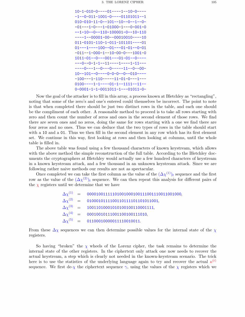
3. THE LORENZ CIPHER 105
10-1-010-0----01----1--10-0-----1--0-011-1001-0----01101011--1010-010-11-0--101--10--0--1--0--01---1-0---1-01000-1---0-001-0--1-10--0--110-100001-0--10-110----1--00001-00--00010010----10011-0101-110-1-011-101101----0101---1----100--01---01-01--0-01-011--1-000-1--10-00-0---1001-01011-01--0---001---01-01--0-------0--0-1-1--11----1----1-11-------0---1--0---0-----11--0--00-10--101--0----0-0-0--0--010-----100---1-110-----11-01-0---1---0100----1-1----01-1--1111--11--0-0001-1-1-0011011-1---01011-0-
Now the goal of the attacker is to fill in this array, a process known at Bletchley as “rectangling”,noting that some of the zero’s and one’s entered could themselves be incorrect. The point to noteis that when completed there should be just two distinct rows in the table, and each one shouldbe the compliment of each other. A reasonable method to proceed is to take all rows starting withzero and then count the number of zeros and ones in the second element of those rows. We findthere are seven ones and no zeros, doing the same for rows starting with a one we find there arefour zeros and no ones. Thus we can deduce that the two types of rows in the table should startwith a 10 and a 01. Thus we then fill in the second element in any row which has its first elementset. We continue in this way, first looking at rows and then looking at columns, until the wholetable is filled in.
The above table was found using a few thousand characters of known keystream, which allowswith the above method the simple reconstruction of the full table. According to the Bletchley doc-uments the cryptographers at Bletchley would actually use a few hundred characters of keystreamin a known keystream attack, and a few thousand in an unknown keystream attack. Since we arefollowing rather naive methods our results are not as spectacular.
Once completed we can take the first column as the value of the (Δχ(1))t sequence and the firstrow as the value of the (Δχ(2))t sequence. We can then repeat this analysis for different pairs ofthe χ registers until we determine that we have
Δχ(1) = 00001001111101001000100111001110011001000,
Δχ(2) = 0100010111100110111101101011001,
Δχ(3) = 10011010001010100100110001111,
Δχ(4) = 00010010111001100100111010,
Δχ(5) = 01100010000011110010011.
From these Δχ sequences we can then determine possible values for the internal state of the χregisters.
So having “broken” the χ wheels of the Lorenz cipher, the task remains to determine theinternal state of the other registers. In the ciphertext only attack one now needs to recover theactual keystream, a step which is clearly not needed in the known-keystream scenario. The trickhere is to use the statistics of the underlying language again to try and recover the actual κ(i)
sequence. We first de-χ the ciphertext sequence γ, using the values of the χ registers which we
106 6. HISTORICAL STREAM CIPHERS
have just determined, to obtain
β(i)t = γ
(i)t ⊕ χ
(i)t
= φ(i)t ⊕ ψ′(i)
t .
We then take the Δ of this β sequence
(Δβ)t = (Δφ)t ⊕(μ′(2)t · (Δψ)tψ
),
and by our previous argument we will see that many values of the Δφ sequence will be “exposed” inthe Δβ sequence. Using the knowledge of the Δφ sequence, e.g. it uses Baudot codes and naturallanguage has many sequences of bigrams (e.g. space always following full stop), one can eventuallyrecover the sequence φ and hence κ. At Bletchley this last step was usually performed by hand.
So in both scenarios we now have determined both the χ and the κ sequences. But what we arereally after was the initial value of the registers ψ and μ. To determine these we de-χ the resultingκ sequence to obtain the ψ′
t sequence. In our example this would reveal the sequence
101100001111111010010100110101111111111110000011010101101010110100101000000101010111011010000000000001111100101011000101101000001000000011010101010100000000000000000011011010111010010100110111111010100001010100000000000001111111011010100110010100101000000101010101101010000000000000000011001101010010
given earlier. From this we can then recover a guess as to the μ′(2)t sequence.
11110111100000111111111111111000000000001000010111111111111...
Note, this is only a guess since it might occur that ψtψ = ψtψ+1, but we shall ignore this
possibility. Once we have determined enough of the μ′(2)t sequence so that we have 59 ones in it,then we will have determined the initial state of the ψ registers. This is because after 59 clock ticksof the ψ registers all outputs have been presented in the ψ′ sequence, since the largest ψ registerhas size 59.
All that remains is to determine the state of the μ registers. To do this we notice that theμ′(2)t sequence will make a transition from a 0 to a 1, or a 1 to a 0, precisely when μ
(1)t outputs a
one. By constructing enough of the μ′(2)t stream as above (say a few hundred bits) this allows usto determine the value of μ(1) register almost exactly. Having recovered μ
(1)t we can then deduce
the values which must be contained in μ(2)tμ from this sequence and the resulting value of μ′(2)t .
According to various documents in the early stages of the Lorenz cipher breaking effort atBletchley, the entire “Wheel Breaking” operation was performed by hand. However, as time pro-gressed the part which involved determining the Δχ sequences above from the rectangling procedurewas eventually performed by the Colossus computer.
3.4. Breaking a Message. The Colossus computer was originally created not to break thewheels, i.e. to determine the longterm key of the Lorenz cipher. The Colossus was originally builtto determine the per message settings, and hence to help break the individual ciphertexts. Whilstthe previous method for breaking the wheels could be used to attack any ciphertext, to make itwork efficiently you require a large ciphertext and a lot of luck. However, once the wheels arebroken, i.e. we know the bits in the various registers, breaking the next ciphertext becomes easier.
Again we use the trick of de-χ’ing the ciphertext sequence γ, and then applying the Δ methodto the resulting sequence β. We assume we know the internal states of all the registers but not theirstarting positions. We shall let si denote the unknown values of the starting positions of the five χ
Further Reading 107
wheels and sφ (resp. sμ) the global unknown starting position of the set of φ (resp. μ) wheels.
βt = γt ⊕ χt+sp
= φt ⊕ ψ′t+sφ ,
and then(Δβ)t = (Δφ)t+sφ ⊕
(μ′(2)t+sμ ·(Δψ)tψ
).
We then take two of the resulting five bit streams and xor them together as before to obtain
(α(i,j))t = (Δβ(i))t ⊕ (Δβ(j))t
= (Δφ(i))t+sφ ⊕ (Δφ(j))t+sφ ⊕ μ′(2)t+tμ((Δψ(i))tψ ⊕ (Δψ(j))tψ
).
Using our prior probability estimates we can determine the following probability estimate
Pr[(α(i,j))t = 0] ≈ 1/2 + ρ · (2 · ε− 1),
which is exactly the same probability we had for Equation 9 holding. In particular we note thatPr[α(i,j)
t = 0] > 1/2, which forms the basis of this method of breaking into Lorenz ciphertexts.Lets fix on i = 1 and j = 2. On assuming we know the values for the registers, all we need do is
determine their starting positions s1, s2. We simply need to go through all 1271 = 41 · 31 possiblestarting positions for the first and second χ register. For each one of these starting positions wecompute the associated (α(1,2))t sequence and count the number of values which are zero. Since wehave Pr[α(i,j)
t = 0] > 1/2 the correct value for the starting positions will correspond to a particularlyhigh value for the count of the number of zeros.
This is a simple statistical test which allows one to determine the start positions of the firstand second χ registers. Repeating this for other pairs of registers, or using similar statisticaltechniques, we can recover the start position of all χ registers. These statistical techniques arewhat the Colossus computer was designed to perform.
Once the χ register positions have been determined, the determination of the start positionsof the ψ and μ registers was then performed by hand. The techniques for this are very similar tothe earlier techniques needed to break the wheels, however once again various simplifications occursince one is assumed to know the state of each register, but not its start position.
Chapter Summary
• We have described the general model for symmetric ciphers, and stream ciphers in partic-ular.
• We have looked at the Vernam cipher as a stream cipher, and described it’s inner workingsin terms of shift registers.
• We sketched how the Lorenz cipher was eventually broken. In particular you shouldnotice that very tiny deviations from true randomness in the output can be exploited bya cryptographer in breaking a stream cipher.
Further Reading
The paper by Carter provides a more detailed description of the cryptanalysis performed atBletchley on the Lorenz cipher. The book by Gannon is a very readable account of the entire
108 6. HISTORICAL STREAM CIPHERS
operation related to the Lorenz cipher, from obtaining the signals through to the construction andoperation of the Colossus computer. For the “real” details you should consult the General Reporton Tunny.
F.L. Carter. The Breaking of the Lorenz Cipher: An Introduction to the Theory Behind the Opera-tional Role of “Colossus” at BP. In Coding and Cryptography - 1997, Springer-Verlag LNCS 1355,74–88, 1997.
P. Gannon Colossus: Bletchley Park’s Greatest Secret. Atlantic Books, 2007.
J. Good, D. Michie and G. Timms. General report on Tunny, With Emphasis on Statistical Methods.Document reference HW 25/4 and HW 25/5, Public Record Office Kew. Originally written in 1945,declassified in 2000.
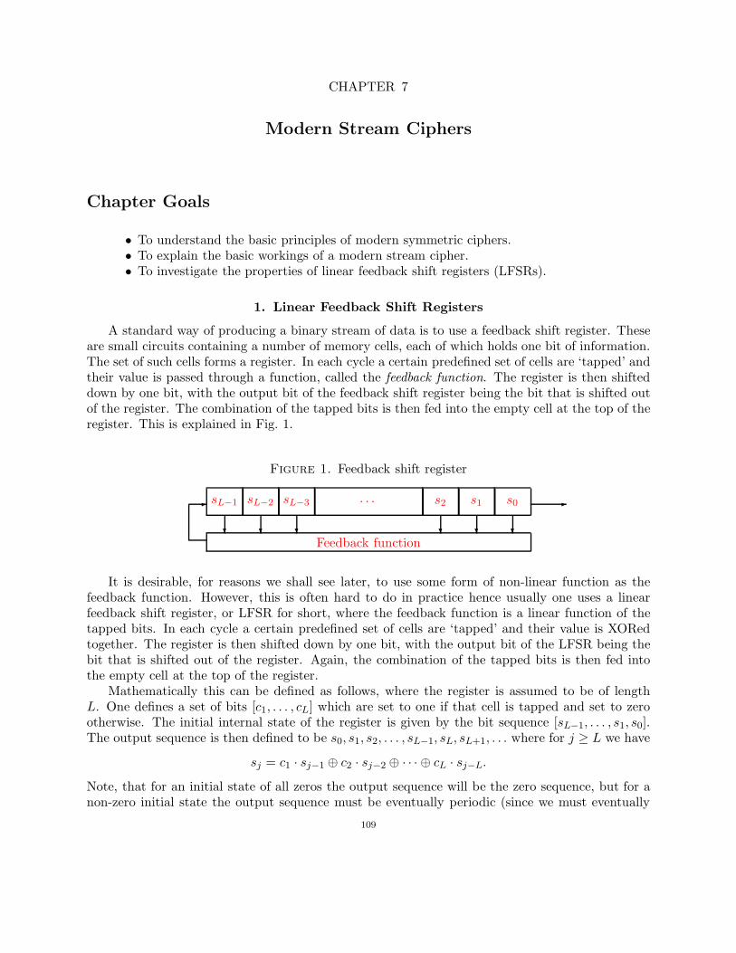
CHAPTER 7
Modern Stream Ciphers
Chapter Goals
• To understand the basic principles of modern symmetric ciphers.• To explain the basic workings of a modern stream cipher.• To investigate the properties of linear feedback shift registers (LFSRs).
1. Linear Feedback Shift Registers
A standard way of producing a binary stream of data is to use a feedback shift register. Theseare small circuits containing a number of memory cells, each of which holds one bit of information.The set of such cells forms a register. In each cycle a certain predefined set of cells are ‘tapped’ andtheir value is passed through a function, called the feedback function. The register is then shifteddown by one bit, with the output bit of the feedback shift register being the bit that is shifted outof the register. The combination of the tapped bits is then fed into the empty cell at the top of theregister. This is explained in Fig. 1.
Figure 1. Feedback shift register
Feedback function
sL−1
sL−2
sL−3
· · · s2
s1
s0
It is desirable, for reasons we shall see later, to use some form of non-linear function as thefeedback function. However, this is often hard to do in practice hence usually one uses a linearfeedback shift register, or LFSR for short, where the feedback function is a linear function of thetapped bits. In each cycle a certain predefined set of cells are ‘tapped’ and their value is XORedtogether. The register is then shifted down by one bit, with the output bit of the LFSR being thebit that is shifted out of the register. Again, the combination of the tapped bits is then fed intothe empty cell at the top of the register.
Mathematically this can be defined as follows, where the register is assumed to be of lengthL. One defines a set of bits [c1, . . . , cL] which are set to one if that cell is tapped and set to zerootherwise. The initial internal state of the register is given by the bit sequence [sL−1, . . . , s1, s0].The output sequence is then defined to be s0, s1, s2, . . . , sL−1, sL, sL+1, . . . where for j ≥ L we have
sj = c1 · sj−1 ⊕ c2 · sj−2 ⊕ · · · ⊕ cL · sj−L.Note, that for an initial state of all zeros the output sequence will be the zero sequence, but for anon-zero initial state the output sequence must be eventually periodic (since we must eventually
109
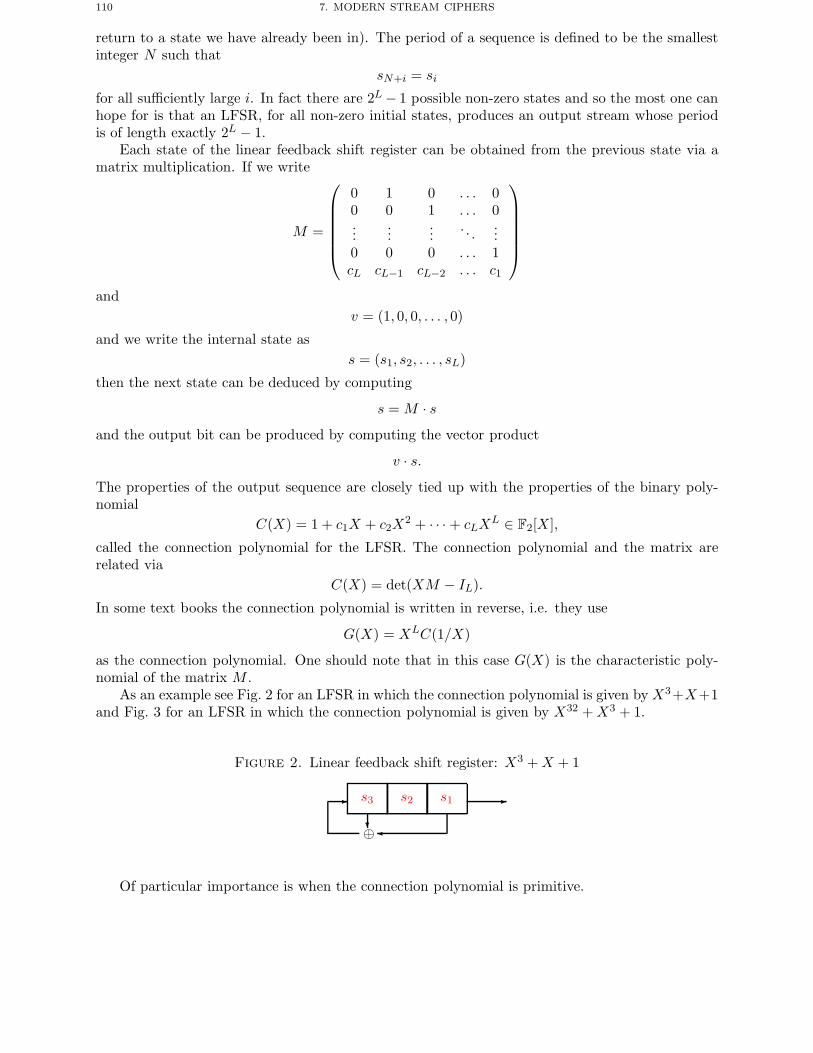
110 7. MODERN STREAM CIPHERS
return to a state we have already been in). The period of a sequence is defined to be the smallestinteger N such that
sN+i = si
for all sufficiently large i. In fact there are 2L− 1 possible non-zero states and so the most one canhope for is that an LFSR, for all non-zero initial states, produces an output stream whose periodis of length exactly 2L − 1.
Each state of the linear feedback shift register can be obtained from the previous state via amatrix multiplication. If we write
M =
⎛⎜⎜⎜⎜⎜⎝
0 1 0 . . . 00 0 1 . . . 0...
......
. . ....
0 0 0 . . . 1cL cL−1 cL−2 . . . c1
⎞⎟⎟⎟⎟⎟⎠
andv = (1, 0, 0, . . . , 0)
and we write the internal state ass = (s1, s2, . . . , sL)
then the next state can be deduced by computing
s = M · sand the output bit can be produced by computing the vector product
v · s.The properties of the output sequence are closely tied up with the properties of the binary poly-nomial
C(X) = 1 + c1X + c2X2 + · · · + cLX
L ∈ F2[X],
called the connection polynomial for the LFSR. The connection polynomial and the matrix arerelated via
C(X) = det(XM − IL).
In some text books the connection polynomial is written in reverse, i.e. they use
G(X) = XLC(1/X)
as the connection polynomial. One should note that in this case G(X) is the characteristic poly-nomial of the matrix M .
As an example see Fig. 2 for an LFSR in which the connection polynomial is given by X3+X+1and Fig. 3 for an LFSR in which the connection polynomial is given by X32 +X3 + 1.
Figure 2. Linear feedback shift register: X3 +X + 1
s3
⊕
s2 s1
�
Of particular importance is when the connection polynomial is primitive.
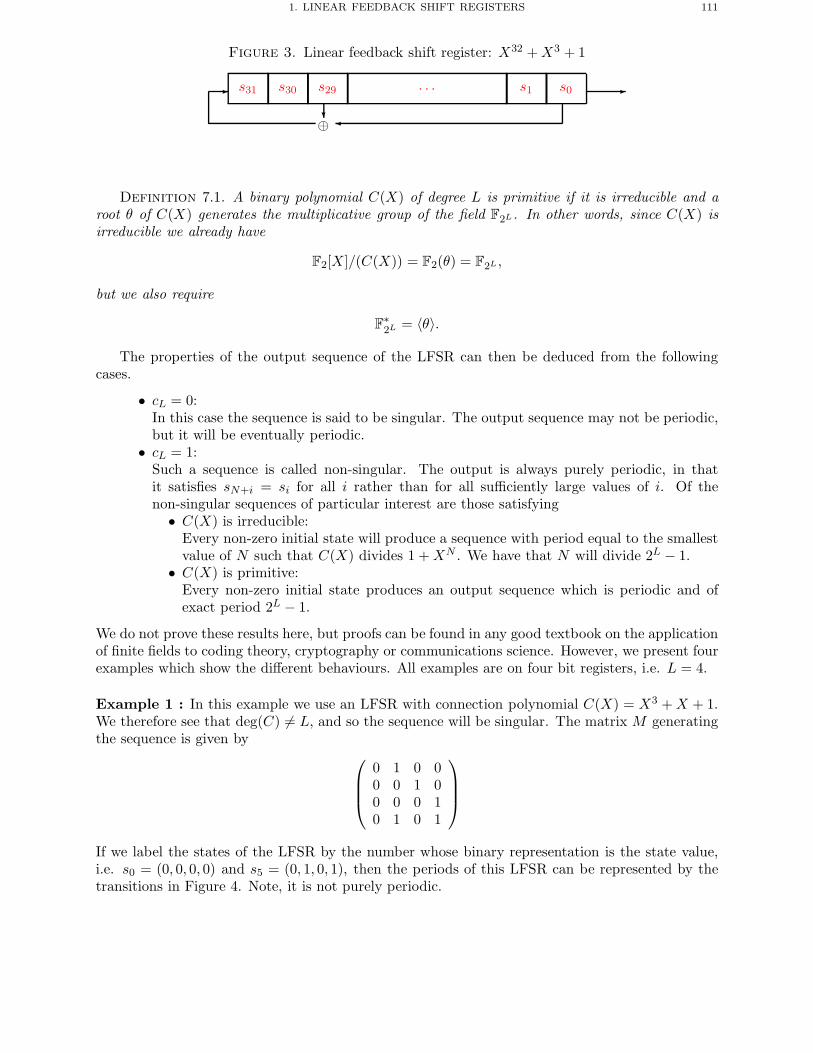
1. LINEAR FEEDBACK SHIFT REGISTERS 111
Figure 3. Linear feedback shift register: X32 +X3 + 1
s31 s30 s29
⊕
. . . s1 s0
�
Definition 7.1. A binary polynomial C(X) of degree L is primitive if it is irreducible and aroot θ of C(X) generates the multiplicative group of the field F2L. In other words, since C(X) isirreducible we already have
F2[X]/(C(X)) = F2(θ) = F2L ,
but we also require
F∗2L = 〈θ〉.
The properties of the output sequence of the LFSR can then be deduced from the followingcases.
• cL = 0:In this case the sequence is said to be singular. The output sequence may not be periodic,but it will be eventually periodic.
• cL = 1:Such a sequence is called non-singular. The output is always purely periodic, in thatit satisfies sN+i = si for all i rather than for all sufficiently large values of i. Of thenon-singular sequences of particular interest are those satisfying
• C(X) is irreducible:Every non-zero initial state will produce a sequence with period equal to the smallestvalue of N such that C(X) divides 1 +XN . We have that N will divide 2L − 1.
• C(X) is primitive:Every non-zero initial state produces an output sequence which is periodic and ofexact period 2L − 1.
We do not prove these results here, but proofs can be found in any good textbook on the applicationof finite fields to coding theory, cryptography or communications science. However, we present fourexamples which show the different behaviours. All examples are on four bit registers, i.e. L = 4.
Example 1 : In this example we use an LFSR with connection polynomial C(X) = X3 +X + 1.We therefore see that deg(C) �= L, and so the sequence will be singular. The matrix M generatingthe sequence is given by ⎛
⎜⎜⎝0 1 0 00 0 1 00 0 0 10 1 0 1
⎞⎟⎟⎠
If we label the states of the LFSR by the number whose binary representation is the state value,i.e. s0 = (0, 0, 0, 0) and s5 = (0, 1, 0, 1), then the periods of this LFSR can be represented by thetransitions in Figure 4. Note, it is not purely periodic.
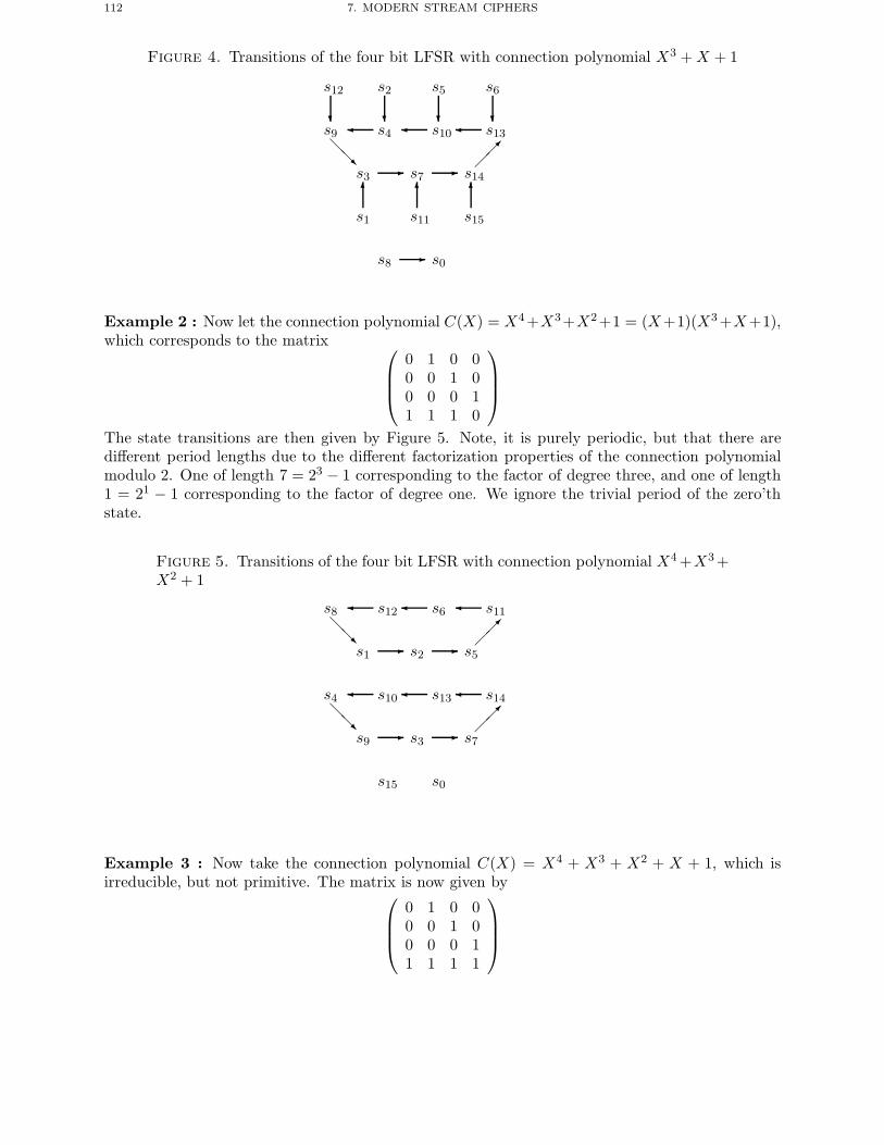
112 7. MODERN STREAM CIPHERS
Figure 4. Transitions of the four bit LFSR with connection polynomial X3 +X + 1
s12
s2
s5
s6
s9
�
s4� s10� s13�
s3 s7 s14�
��
s1
�
s11
�
s15
�
s8 s0
Example 2 : Now let the connection polynomial C(X) = X4+X3+X2+1 = (X+1)(X3 +X+1),which corresponds to the matrix ⎛
⎜⎜⎝0 1 0 00 0 1 00 0 0 11 1 1 0
⎞⎟⎟⎠
The state transitions are then given by Figure 5. Note, it is purely periodic, but that there aredifferent period lengths due to the different factorization properties of the connection polynomialmodulo 2. One of length 7 = 23 − 1 corresponding to the factor of degree three, and one of length1 = 21 − 1 corresponding to the factor of degree one. We ignore the trivial period of the zero’thstate.
Figure 5. Transitions of the four bit LFSR with connection polynomial X4 +X3 +X2 + 1
s8
�
s12� s6� s11�
s1 s2 s5�
��
s4
�
s10� s13� s14�
s9 s3 s7�
��
s15 s0
Example 3 : Now take the connection polynomial C(X) = X4 + X3 + X2 + X + 1, which isirreducible, but not primitive. The matrix is now given by⎛
⎜⎜⎝0 1 0 00 0 1 00 0 0 11 1 1 1
⎞⎟⎟⎠
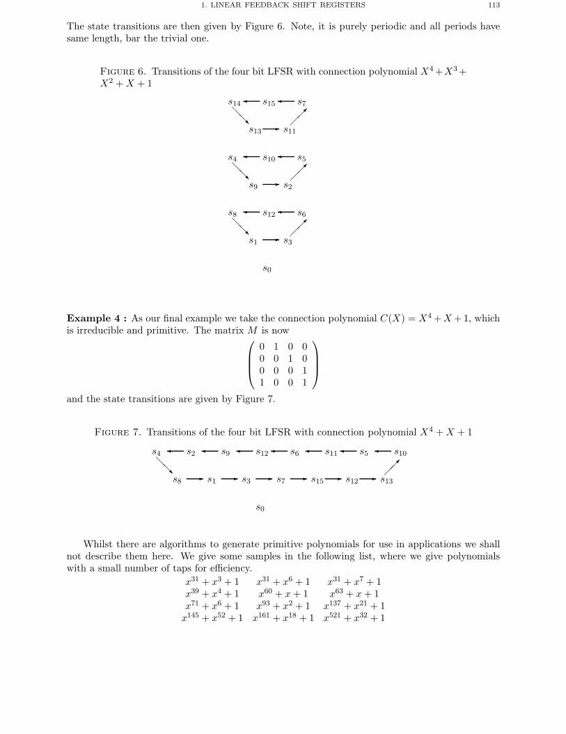
1. LINEAR FEEDBACK SHIFT REGISTERS 113
The state transitions are then given by Figure 6. Note, it is purely periodic and all periods havesame length, bar the trivial one.
Figure 6. Transitions of the four bit LFSR with connection polynomial X4 +X3 +X2 +X + 1
s14
�
s15� s7�
s13 s11�
��
s4
�
s10� s5�
s9 s2�
��
s8
�
s12� s6�
s1 s3�
��
s0
Example 4 : As our final example we take the connection polynomial C(X) = X4 +X+ 1, whichis irreducible and primitive. The matrix M is now⎛
⎜⎜⎝0 1 0 00 0 1 00 0 0 11 0 0 1
⎞⎟⎟⎠
and the state transitions are given by Figure 7.
Figure 7. Transitions of the four bit LFSR with connection polynomial X4 +X + 1
s4
�
s2� s9� s12� s6� s11� s5� s10�
s8 s1 s3 s7 s15 s12 s13���
s0
Whilst there are algorithms to generate primitive polynomials for use in applications we shallnot describe them here. We give some samples in the following list, where we give polynomialswith a small number of taps for efficiency.
x31 + x3 + 1 x31 + x6 + 1 x31 + x7 + 1x39 + x4 + 1 x60 + x+ 1 x63 + x+ 1x71 + x6 + 1 x93 + x2 + 1 x137 + x21 + 1x145 + x52 + 1 x161 + x18 + 1 x521 + x32 + 1
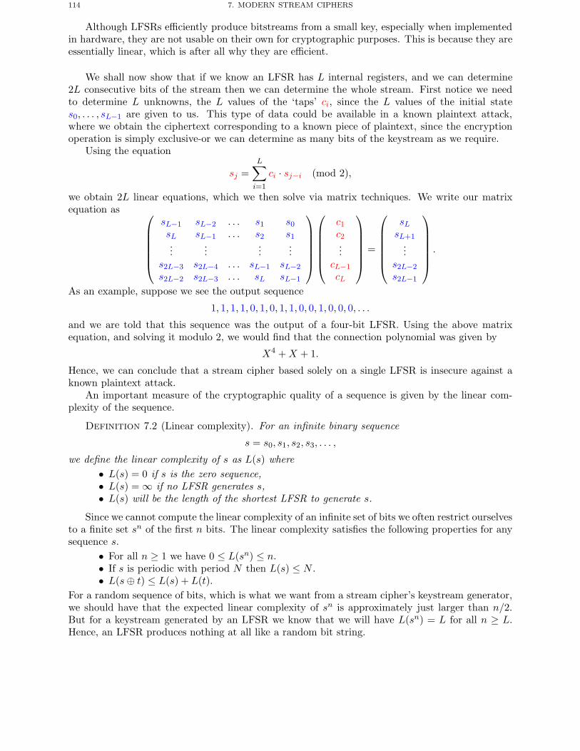
114 7. MODERN STREAM CIPHERS
Although LFSRs efficiently produce bitstreams from a small key, especially when implementedin hardware, they are not usable on their own for cryptographic purposes. This is because they areessentially linear, which is after all why they are efficient.
We shall now show that if we know an LFSR has L internal registers, and we can determine2L consecutive bits of the stream then we can determine the whole stream. First notice we needto determine L unknowns, the L values of the ‘taps’ ci, since the L values of the initial states0, . . . , sL−1 are given to us. This type of data could be available in a known plaintext attack,where we obtain the ciphertext corresponding to a known piece of plaintext, since the encryptionoperation is simply exclusive-or we can determine as many bits of the keystream as we require.
Using the equation
sj =L∑i=1
ci · sj−i (mod 2),
we obtain 2L linear equations, which we then solve via matrix techniques. We write our matrixequation as ⎛
⎜⎜⎜⎜⎜⎝
sL−1 sL−2 . . . s1 s0sL sL−1 . . . s2 s1...
......
...s2L−3 s2L−4 . . . sL−1 sL−2
s2L−2 s2L−3 . . . sL sL−1
⎞⎟⎟⎟⎟⎟⎠
⎛⎜⎜⎜⎜⎜⎝
c1c2...
cL−1
cL
⎞⎟⎟⎟⎟⎟⎠ =
⎛⎜⎜⎜⎜⎜⎝
sLsL+1
...s2L−2
s2L−1
⎞⎟⎟⎟⎟⎟⎠ .
As an example, suppose we see the output sequence
1, 1, 1, 1, 0, 1, 0, 1, 1, 0, 0, 1, 0, 0, 0, . . .
and we are told that this sequence was the output of a four-bit LFSR. Using the above matrixequation, and solving it modulo 2, we would find that the connection polynomial was given by
X4 +X + 1.
Hence, we can conclude that a stream cipher based solely on a single LFSR is insecure against aknown plaintext attack.
An important measure of the cryptographic quality of a sequence is given by the linear com-plexity of the sequence.
Definition 7.2 (Linear complexity). For an infinite binary sequence
s = s0, s1, s2, s3, . . . ,
we define the linear complexity of s as L(s) where• L(s) = 0 if s is the zero sequence,• L(s) = ∞ if no LFSR generates s,• L(s) will be the length of the shortest LFSR to generate s.
Since we cannot compute the linear complexity of an infinite set of bits we often restrict ourselvesto a finite set sn of the first n bits. The linear complexity satisfies the following properties for anysequence s.
• For all n ≥ 1 we have 0 ≤ L(sn) ≤ n.• If s is periodic with period N then L(s) ≤ N .• L(s⊕ t) ≤ L(s) + L(t).
For a random sequence of bits, which is what we want from a stream cipher’s keystream generator,we should have that the expected linear complexity of sn is approximately just larger than n/2.But for a keystream generated by an LFSR we know that we will have L(sn) = L for all n ≥ L.Hence, an LFSR produces nothing at all like a random bit string.
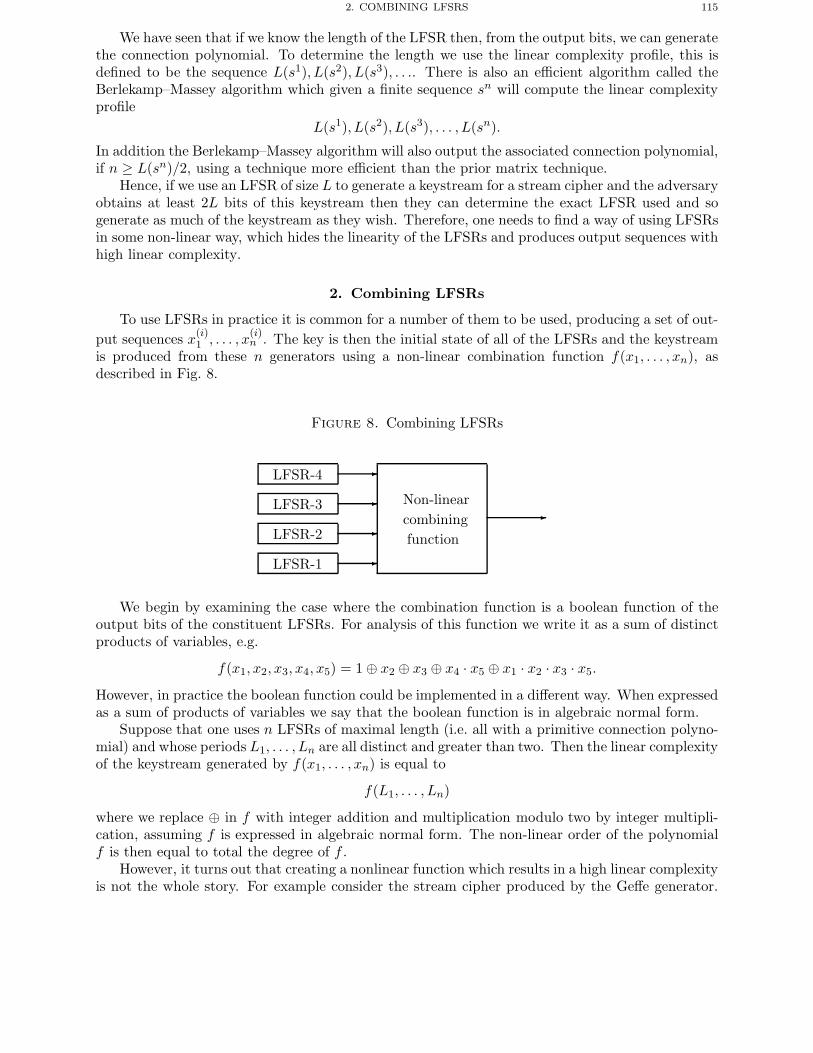
2. COMBINING LFSRS 115
We have seen that if we know the length of the LFSR then, from the output bits, we can generatethe connection polynomial. To determine the length we use the linear complexity profile, this isdefined to be the sequence L(s1), L(s2), L(s3), . . .. There is also an efficient algorithm called theBerlekamp–Massey algorithm which given a finite sequence sn will compute the linear complexityprofile
L(s1), L(s2), L(s3), . . . , L(sn).
In addition the Berlekamp–Massey algorithm will also output the associated connection polynomial,if n ≥ L(sn)/2, using a technique more efficient than the prior matrix technique.
Hence, if we use an LFSR of size L to generate a keystream for a stream cipher and the adversaryobtains at least 2L bits of this keystream then they can determine the exact LFSR used and sogenerate as much of the keystream as they wish. Therefore, one needs to find a way of using LFSRsin some non-linear way, which hides the linearity of the LFSRs and produces output sequences withhigh linear complexity.
2. Combining LFSRs
To use LFSRs in practice it is common for a number of them to be used, producing a set of out-put sequences x(i)
1 , . . . , x(i)n . The key is then the initial state of all of the LFSRs and the keystream
is produced from these n generators using a non-linear combination function f(x1, . . . , xn), asdescribed in Fig. 8.
Figure 8. Combining LFSRs
LFSR-1
LFSR-2
LFSR-3
LFSR-4
Non-linearcombiningfunction
We begin by examining the case where the combination function is a boolean function of theoutput bits of the constituent LFSRs. For analysis of this function we write it as a sum of distinctproducts of variables, e.g.
f(x1, x2, x3, x4, x5) = 1 ⊕ x2 ⊕ x3 ⊕ x4 · x5 ⊕ x1 · x2 · x3 · x5.
However, in practice the boolean function could be implemented in a different way. When expressedas a sum of products of variables we say that the boolean function is in algebraic normal form.
Suppose that one uses n LFSRs of maximal length (i.e. all with a primitive connection polyno-mial) and whose periods L1, . . . , Ln are all distinct and greater than two. Then the linear complexityof the keystream generated by f(x1, . . . , xn) is equal to
f(L1, . . . , Ln)
where we replace ⊕ in f with integer addition and multiplication modulo two by integer multipli-cation, assuming f is expressed in algebraic normal form. The non-linear order of the polynomialf is then equal to total the degree of f .
However, it turns out that creating a nonlinear function which results in a high linear complexityis not the whole story. For example consider the stream cipher produced by the Geffe generator.
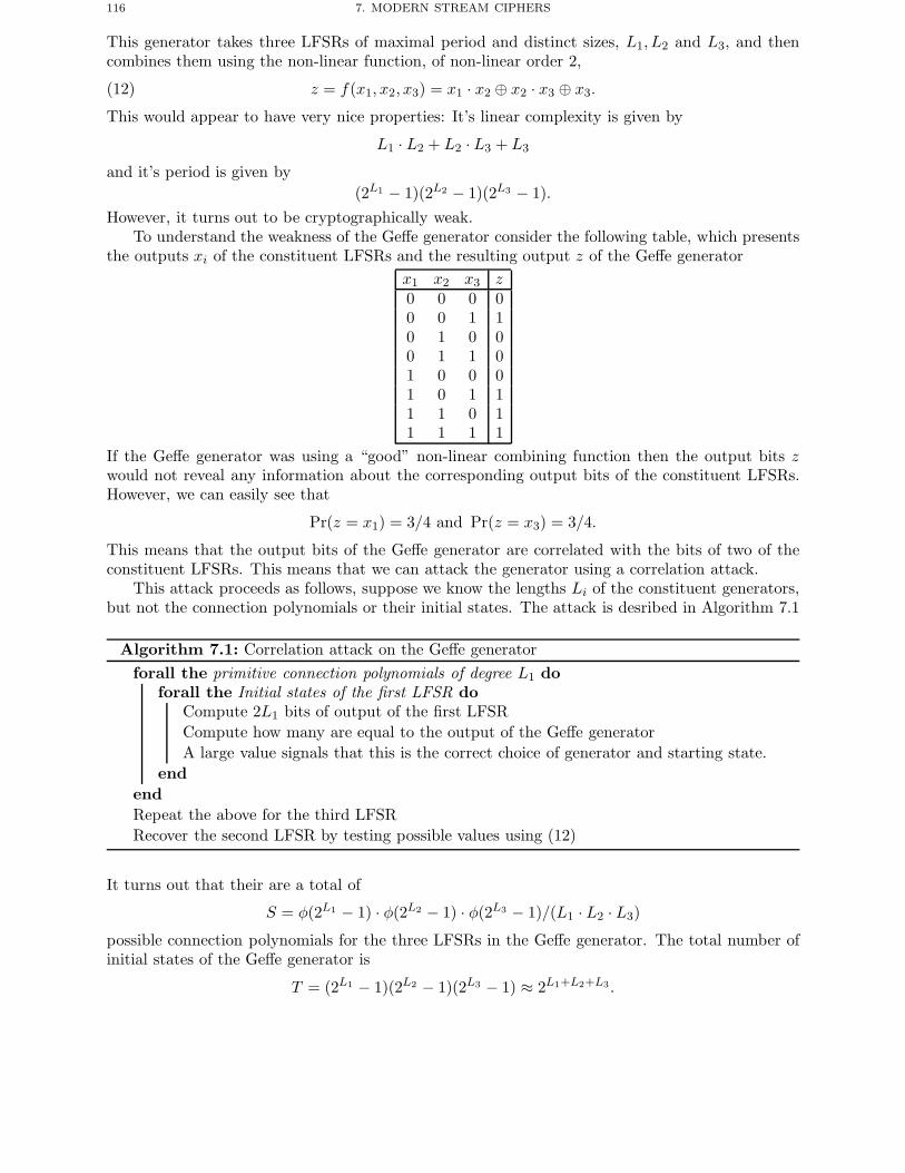
116 7. MODERN STREAM CIPHERS
This generator takes three LFSRs of maximal period and distinct sizes, L1, L2 and L3, and thencombines them using the non-linear function, of non-linear order 2,
(12) z = f(x1, x2, x3) = x1 · x2 ⊕ x2 · x3 ⊕ x3.
This would appear to have very nice properties: It’s linear complexity is given by
L1 · L2 + L2 · L3 + L3
and it’s period is given by(2L1 − 1)(2L2 − 1)(2L3 − 1).
However, it turns out to be cryptographically weak.To understand the weakness of the Geffe generator consider the following table, which presents
the outputs xi of the constituent LFSRs and the resulting output z of the Geffe generatorx1 x2 x3 z0 0 0 00 0 1 10 1 0 00 1 1 01 0 0 01 0 1 11 1 0 11 1 1 1
If the Geffe generator was using a “good” non-linear combining function then the output bits zwould not reveal any information about the corresponding output bits of the constituent LFSRs.However, we can easily see that
Pr(z = x1) = 3/4 and Pr(z = x3) = 3/4.
This means that the output bits of the Geffe generator are correlated with the bits of two of theconstituent LFSRs. This means that we can attack the generator using a correlation attack.
This attack proceeds as follows, suppose we know the lengths Li of the constituent generators,but not the connection polynomials or their initial states. The attack is desribed in Algorithm 7.1
Algorithm 7.1: Correlation attack on the Geffe generatorforall the primitive connection polynomials of degree L1 do
forall the Initial states of the first LFSR doCompute 2L1 bits of output of the first LFSRCompute how many are equal to the output of the Geffe generatorA large value signals that this is the correct choice of generator and starting state.
endendRepeat the above for the third LFSRRecover the second LFSR by testing possible values using (12)
It turns out that their are a total of
S = φ(2L1 − 1) · φ(2L2 − 1) · φ(2L3 − 1)/(L1 · L2 · L3)
possible connection polynomials for the three LFSRs in the Geffe generator. The total number ofinitial states of the Geffe generator is
T = (2L1 − 1)(2L2 − 1)(2L3 − 1) ≈ 2L1+L2+L3.
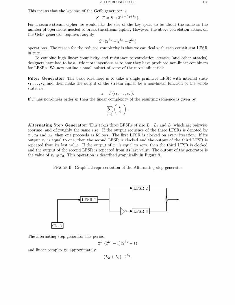
2. COMBINING LFSRS 117
This means that the key size of the Geffe generator is
S · T ≈ S · (2L1+L2+L3).
For a secure stream cipher we would like the size of the key space to be about the same as thenumber of operations needed to break the stream cipher. However, the above correlation attack onthe Geffe generator requires roughly
S · (2L1 + 2L2 + 2L3)
operations. The reason for the reduced complexity is that we can deal with each constituent LFSRin turn.
To combine high linear complexity and resistance to correlation attacks (and other attacks)designers have had to be a little more ingenious as to how they have produced non-linear combinersfor LFSRs. We now outline a small subset of some of the most influential:
Filter Generator: The basic idea here is to take a single primitive LFSR with internal states1, . . . , sL and then make the output of the stream cipher be a non-linear function of the wholestate, i.e.
z = F (s1, . . . , sL).If F has non-linear order m then the linear complexity of the resulting sequence is given by
m∑i=1
(Li
).
Alternating Step Generator: This takes three LFSRs of size L1, L2 and L3 which are pairwisecoprime, and of roughly the same size. If the output sequence of the three LFSRs is denoted byx1, x2 and x3, then one proceeds as follows: The first LFSR is clocked on every iteration. If itsoutput x1 is equal to one, then the second LFSR is clocked and the output of the third LFSR isrepeated from its last value. If the output of x1 is equal to zero, then the third LFSR is clockedand the output of the second LFSR is repeated from its last value. The output of the generator isthe value of x2 ⊕ x3. This operation is described graphically in Figure 9.
Figure 9. Graphical representation of the Alternating step generator
Clock
� LFSR 1
� LFSR 2
� LFSR 3 ��
�
�
⊕
The alternating step generator has period
2L1(2L2 − 1)(2L3 − 1)
and linear complexity, approximately
(L2 + L3) · 2L1 .
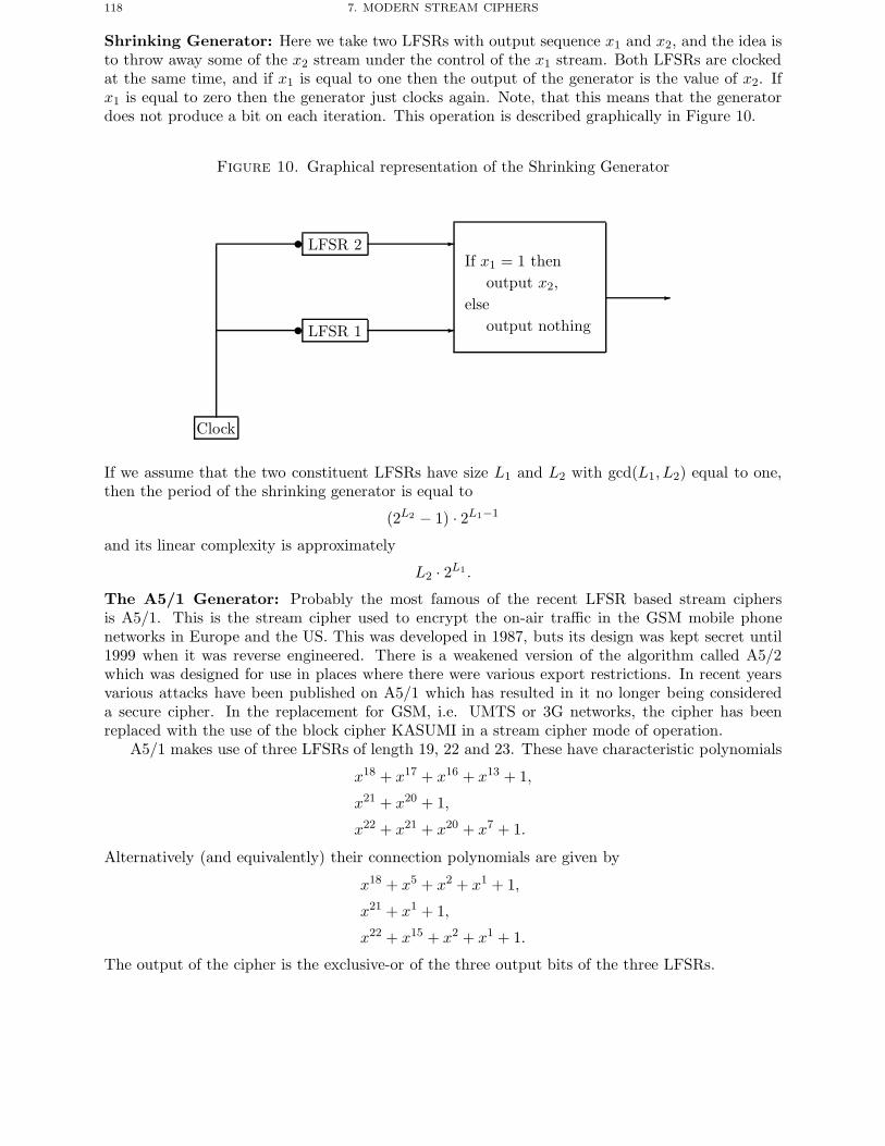
118 7. MODERN STREAM CIPHERS
Shrinking Generator: Here we take two LFSRs with output sequence x1 and x2, and the idea isto throw away some of the x2 stream under the control of the x1 stream. Both LFSRs are clockedat the same time, and if x1 is equal to one then the output of the generator is the value of x2. Ifx1 is equal to zero then the generator just clocks again. Note, that this means that the generatordoes not produce a bit on each iteration. This operation is described graphically in Figure 10.
Figure 10. Graphical representation of the Shrinking Generator
Clock
� LFSR 1
� LFSR 2
If x1 = 1 thenoutput x2,
elseoutput nothing
If we assume that the two constituent LFSRs have size L1 and L2 with gcd(L1, L2) equal to one,then the period of the shrinking generator is equal to
(2L2 − 1) · 2L1−1
and its linear complexity is approximately
L2 · 2L1 .
The A5/1 Generator: Probably the most famous of the recent LFSR based stream ciphersis A5/1. This is the stream cipher used to encrypt the on-air traffic in the GSM mobile phonenetworks in Europe and the US. This was developed in 1987, buts its design was kept secret until1999 when it was reverse engineered. There is a weakened version of the algorithm called A5/2which was designed for use in places where there were various export restrictions. In recent yearsvarious attacks have been published on A5/1 which has resulted in it no longer being considereda secure cipher. In the replacement for GSM, i.e. UMTS or 3G networks, the cipher has beenreplaced with the use of the block cipher KASUMI in a stream cipher mode of operation.
A5/1 makes use of three LFSRs of length 19, 22 and 23. These have characteristic polynomials
x18 + x17 + x16 + x13 + 1,
x21 + x20 + 1,
x22 + x21 + x20 + x7 + 1.
Alternatively (and equivalently) their connection polynomials are given by
x18 + x5 + x2 + x1 + 1,
x21 + x1 + 1,
x22 + x15 + x2 + x1 + 1.
The output of the cipher is the exclusive-or of the three output bits of the three LFSRs.
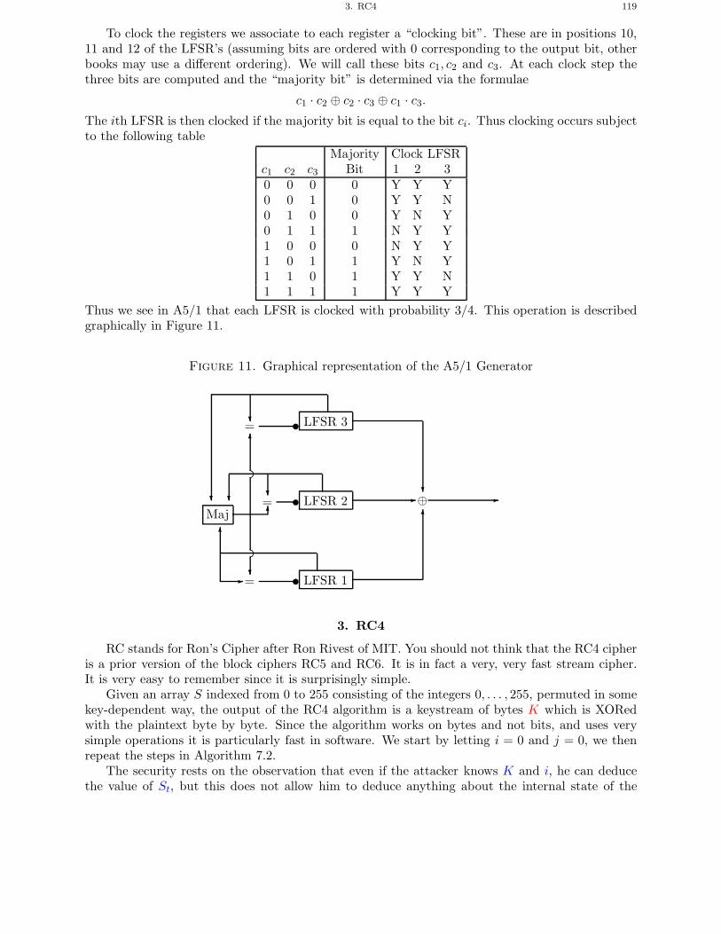
3. RC4 119
To clock the registers we associate to each register a “clocking bit”. These are in positions 10,11 and 12 of the LFSR’s (assuming bits are ordered with 0 corresponding to the output bit, otherbooks may use a different ordering). We will call these bits c1, c2 and c3. At each clock step thethree bits are computed and the “majority bit” is determined via the formulae
c1 · c2 ⊕ c2 · c3 ⊕ c1 · c3.The ith LFSR is then clocked if the majority bit is equal to the bit ci. Thus clocking occurs subjectto the following table
Majority Clock LFSRc1 c2 c3 Bit 1 2 30 0 0 0 Y Y Y0 0 1 0 Y Y N0 1 0 0 Y N Y0 1 1 1 N Y Y1 0 0 0 N Y Y1 0 1 1 Y N Y1 1 0 1 Y Y N1 1 1 1 Y Y Y
Thus we see in A5/1 that each LFSR is clocked with probability 3/4. This operation is describedgraphically in Figure 11.
Figure 11. Graphical representation of the A5/1 Generator
LFSR 1
LFSR 2
LFSR 3
⊕�
�
Maj
.................................
= �
.................................
�= �
�=
�
3. RC4
RC stands for Ron’s Cipher after Ron Rivest of MIT. You should not think that the RC4 cipheris a prior version of the block ciphers RC5 and RC6. It is in fact a very, very fast stream cipher.It is very easy to remember since it is surprisingly simple.
Given an array S indexed from 0 to 255 consisting of the integers 0, . . . , 255, permuted in somekey-dependent way, the output of the RC4 algorithm is a keystream of bytes K which is XORedwith the plaintext byte by byte. Since the algorithm works on bytes and not bits, and uses verysimple operations it is particularly fast in software. We start by letting i = 0 and j = 0, we thenrepeat the steps in Algorithm 7.2.
The security rests on the observation that even if the attacker knows K and i, he can deducethe value of St, but this does not allow him to deduce anything about the internal state of the
120 7. MODERN STREAM CIPHERS
Algorithm 7.2: RC4 Algorithmi = (i+ 1) mod 256j = (j + Si) mod 256swap(Si, Sj)t = (Si + Sj) mod 256K = St
table. This follows from the observation that he cannot deduce the value of t, as he does not knowj, Si or Sj.
It is a very tightly designed algorithm as each line of the code needs to be there to make thecipher secure.
• i = (i+ 1) mod 256 :Makes sure every array element is used once after 256 iterations.
• j = (j + Si) mod 256 :Makes the output depend non-linearly on the array.
• swap(Si, Sj) :Makes sure the array is evolved and modified as the iteration continues.
• t = (Si + Sj) mod 256 :Makes sure the output sequence reveals little about the internal state of the array.
The initial state of the array S is determined from the key using the method described by Algorithm7.3.
Algorithm 7.3: RC4 Key Schedulefor i = 0 to 255 do Si = i
Initialise Ki, for i = 0, . . . , 255, with the key, repeating if neccesaryj = 0for i = 0 to 255 do
j = (j + Si +Ki) mod 256swap(Si, Sj)
end
Although RC4 is very fast for a software based stream cipher, there are some issues with its use.In particular both the key schedule and the main algorithm do not produce as random a stream asone might wish. Hence, it should be used with care.
Chapter Summary
• Modern stream ciphers can be obtained by combining, in a non-linear way, simple bitgenerators called LFSRs, these stream ciphers are bit oriented.
• LFSR based stream ciphers provide very fast ciphers, suitable for implementation in hard-ware, which can encrypt real-time data such as voice or video.
• RC4 provides a fast and compact byte oriented stream cipher for use in software.
Further Reading 121
Further Reading
A good introduction to linear recurrence sequences over finite fields is in the book by Lidl andNeiderreiter. This book covers all the theory one requires, including examples and a descriptionof the Berlekamp–Massey algorithm. Analysis of the RC4 algorithm can be found in the Master’sthesis of Mantin.
R. Lidl and H. Neiderreiter. Introduction to fintie field and their applications. Cambridge UniversityPress, 1986.
I. Mantin. Analysis of the Stream Cipher RC4. MSc. Thesis, Weizmann Institute of Science, 2001.

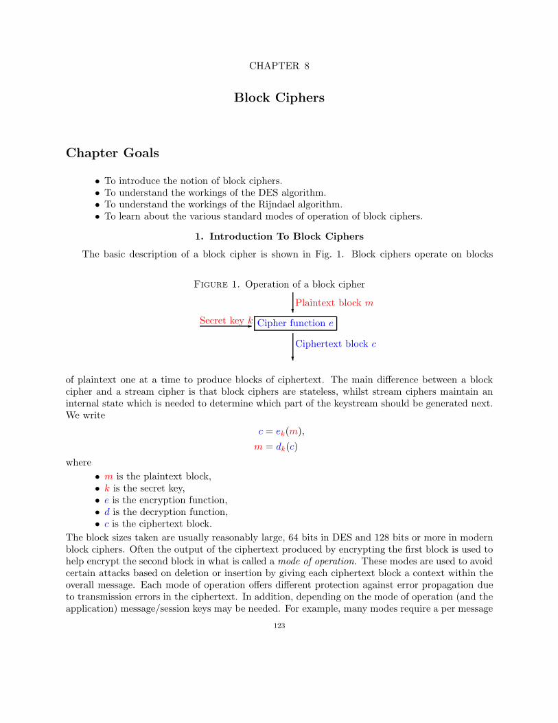
CHAPTER 8
Block Ciphers
Chapter Goals
• To introduce the notion of block ciphers.• To understand the workings of the DES algorithm.• To understand the workings of the Rijndael algorithm.• To learn about the various standard modes of operation of block ciphers.
1. Introduction To Block Ciphers
The basic description of a block cipher is shown in Fig. 1. Block ciphers operate on blocks
Figure 1. Operation of a block cipher
Ciphertext block c
Plaintext block m
Cipher function eSecret key k
of plaintext one at a time to produce blocks of ciphertext. The main difference between a blockcipher and a stream cipher is that block ciphers are stateless, whilst stream ciphers maintain aninternal state which is needed to determine which part of the keystream should be generated next.We write
c = ek(m),
m = dk(c)
where• m is the plaintext block,• k is the secret key,• e is the encryption function,• d is the decryption function,• c is the ciphertext block.
The block sizes taken are usually reasonably large, 64 bits in DES and 128 bits or more in modernblock ciphers. Often the output of the ciphertext produced by encrypting the first block is used tohelp encrypt the second block in what is called a mode of operation. These modes are used to avoidcertain attacks based on deletion or insertion by giving each ciphertext block a context within theoverall message. Each mode of operation offers different protection against error propagation dueto transmission errors in the ciphertext. In addition, depending on the mode of operation (and theapplication) message/session keys may be needed. For example, many modes require a per message
123
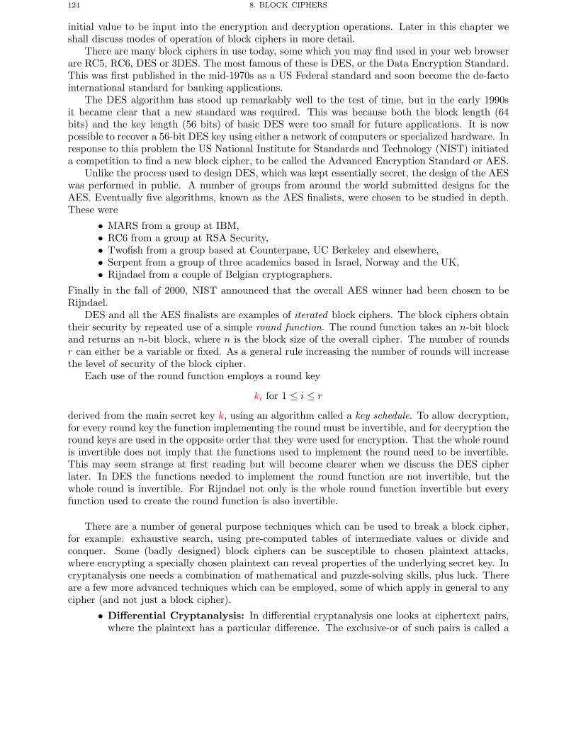
124 8. BLOCK CIPHERS
initial value to be input into the encryption and decryption operations. Later in this chapter weshall discuss modes of operation of block ciphers in more detail.
There are many block ciphers in use today, some which you may find used in your web browserare RC5, RC6, DES or 3DES. The most famous of these is DES, or the Data Encryption Standard.This was first published in the mid-1970s as a US Federal standard and soon become the de-factointernational standard for banking applications.
The DES algorithm has stood up remarkably well to the test of time, but in the early 1990sit became clear that a new standard was required. This was because both the block length (64bits) and the key length (56 bits) of basic DES were too small for future applications. It is nowpossible to recover a 56-bit DES key using either a network of computers or specialized hardware. Inresponse to this problem the US National Institute for Standards and Technology (NIST) initiateda competition to find a new block cipher, to be called the Advanced Encryption Standard or AES.
Unlike the process used to design DES, which was kept essentially secret, the design of the AESwas performed in public. A number of groups from around the world submitted designs for theAES. Eventually five algorithms, known as the AES finalists, were chosen to be studied in depth.These were
• MARS from a group at IBM,• RC6 from a group at RSA Security,• Twofish from a group based at Counterpane, UC Berkeley and elsewhere,• Serpent from a group of three academics based in Israel, Norway and the UK,• Rijndael from a couple of Belgian cryptographers.
Finally in the fall of 2000, NIST announced that the overall AES winner had been chosen to beRijndael.
DES and all the AES finalists are examples of iterated block ciphers. The block ciphers obtaintheir security by repeated use of a simple round function. The round function takes an n-bit blockand returns an n-bit block, where n is the block size of the overall cipher. The number of roundsr can either be a variable or fixed. As a general rule increasing the number of rounds will increasethe level of security of the block cipher.
Each use of the round function employs a round key
ki for 1 ≤ i ≤ r
derived from the main secret key k, using an algorithm called a key schedule. To allow decryption,for every round key the function implementing the round must be invertible, and for decryption theround keys are used in the opposite order that they were used for encryption. That the whole roundis invertible does not imply that the functions used to implement the round need to be invertible.This may seem strange at first reading but will become clearer when we discuss the DES cipherlater. In DES the functions needed to implement the round function are not invertible, but thewhole round is invertible. For Rijndael not only is the whole round function invertible but everyfunction used to create the round function is also invertible.
There are a number of general purpose techniques which can be used to break a block cipher,for example: exhaustive search, using pre-computed tables of intermediate values or divide andconquer. Some (badly designed) block ciphers can be susceptible to chosen plaintext attacks,where encrypting a specially chosen plaintext can reveal properties of the underlying secret key. Incryptanalysis one needs a combination of mathematical and puzzle-solving skills, plus luck. Thereare a few more advanced techniques which can be employed, some of which apply in general to anycipher (and not just a block cipher).
• Differential Cryptanalysis: In differential cryptanalysis one looks at ciphertext pairs,where the plaintext has a particular difference. The exclusive-or of such pairs is called a
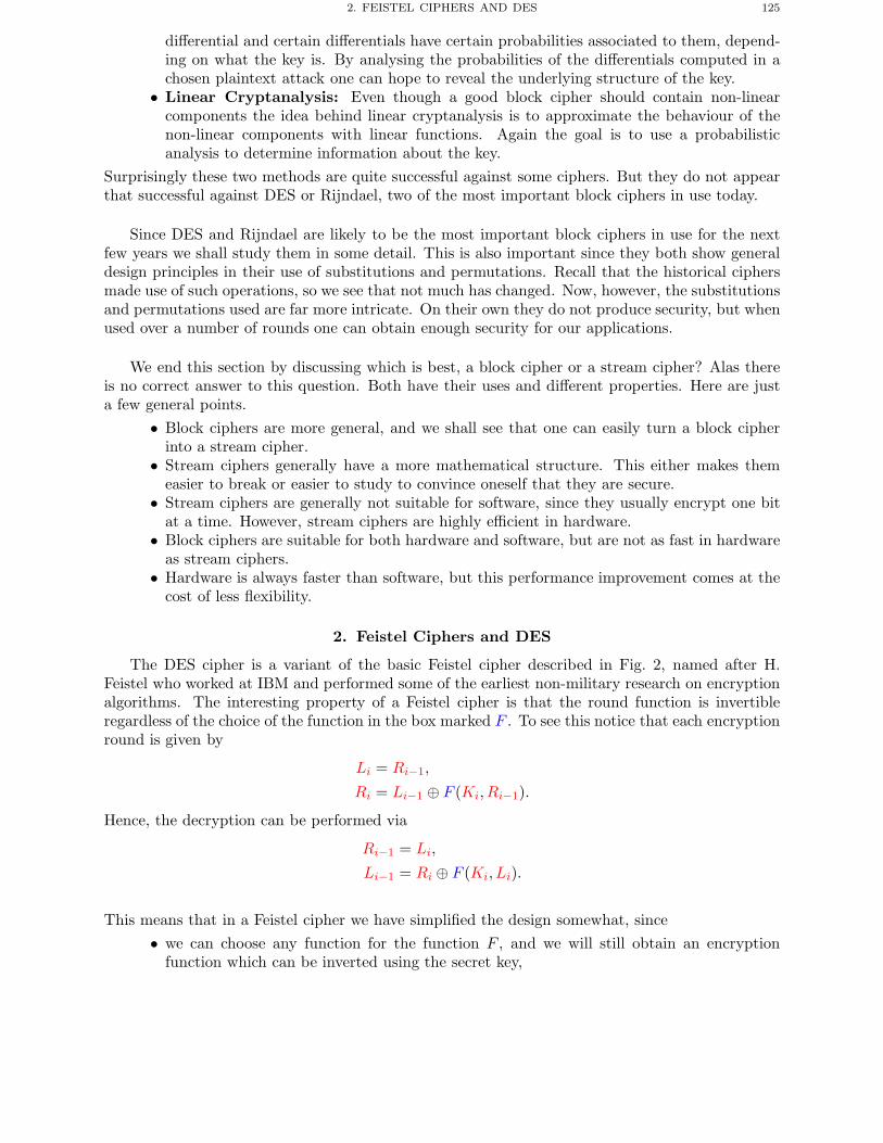
2. FEISTEL CIPHERS AND DES 125
differential and certain differentials have certain probabilities associated to them, depend-ing on what the key is. By analysing the probabilities of the differentials computed in achosen plaintext attack one can hope to reveal the underlying structure of the key.
• Linear Cryptanalysis: Even though a good block cipher should contain non-linearcomponents the idea behind linear cryptanalysis is to approximate the behaviour of thenon-linear components with linear functions. Again the goal is to use a probabilisticanalysis to determine information about the key.
Surprisingly these two methods are quite successful against some ciphers. But they do not appearthat successful against DES or Rijndael, two of the most important block ciphers in use today.
Since DES and Rijndael are likely to be the most important block ciphers in use for the nextfew years we shall study them in some detail. This is also important since they both show generaldesign principles in their use of substitutions and permutations. Recall that the historical ciphersmade use of such operations, so we see that not much has changed. Now, however, the substitutionsand permutations used are far more intricate. On their own they do not produce security, but whenused over a number of rounds one can obtain enough security for our applications.
We end this section by discussing which is best, a block cipher or a stream cipher? Alas thereis no correct answer to this question. Both have their uses and different properties. Here are justa few general points.
• Block ciphers are more general, and we shall see that one can easily turn a block cipherinto a stream cipher.
• Stream ciphers generally have a more mathematical structure. This either makes themeasier to break or easier to study to convince oneself that they are secure.
• Stream ciphers are generally not suitable for software, since they usually encrypt one bitat a time. However, stream ciphers are highly efficient in hardware.
• Block ciphers are suitable for both hardware and software, but are not as fast in hardwareas stream ciphers.
• Hardware is always faster than software, but this performance improvement comes at thecost of less flexibility.
2. Feistel Ciphers and DES
The DES cipher is a variant of the basic Feistel cipher described in Fig. 2, named after H.Feistel who worked at IBM and performed some of the earliest non-military research on encryptionalgorithms. The interesting property of a Feistel cipher is that the round function is invertibleregardless of the choice of the function in the box marked F . To see this notice that each encryptionround is given by
Li = Ri−1,
Ri = Li−1 ⊕ F (Ki, Ri−1).
Hence, the decryption can be performed via
Ri−1 = Li,
Li−1 = Ri ⊕ F (Ki, Li).
This means that in a Feistel cipher we have simplified the design somewhat, since• we can choose any function for the function F , and we will still obtain an encryption
function which can be inverted using the secret key,
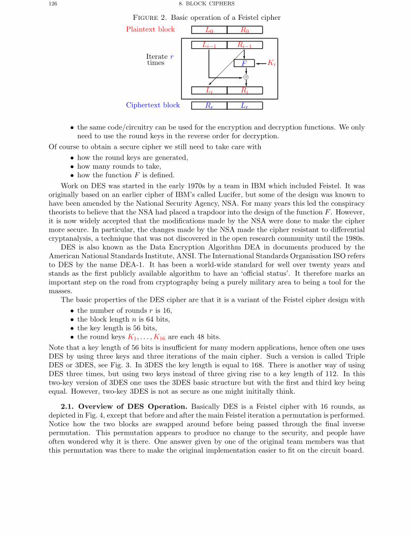
126 8. BLOCK CIPHERS
Figure 2. Basic operation of a Feistel cipher
Plaintext block L0 R0
Iterate rtimes
Li−1 Ri−1
��
��
���
F Ki�
⊕
Li Ri
Ciphertext block Rr Lr
• the same code/circuitry can be used for the encryption and decryption functions. We onlyneed to use the round keys in the reverse order for decryption.
Of course to obtain a secure cipher we still need to take care with• how the round keys are generated,• how many rounds to take,• how the function F is defined.
Work on DES was started in the early 1970s by a team in IBM which included Feistel. It wasoriginally based on an earlier cipher of IBM’s called Lucifer, but some of the design was known tohave been amended by the National Security Agency, NSA. For many years this led the conspiracytheorists to believe that the NSA had placed a trapdoor into the design of the function F . However,it is now widely accepted that the modifications made by the NSA were done to make the ciphermore secure. In particular, the changes made by the NSA made the cipher resistant to differentialcryptanalysis, a technique that was not discovered in the open research community until the 1980s.
DES is also known as the Data Encryption Algorithm DEA in documents produced by theAmerican National Standards Institute, ANSI. The International Standards Organisation ISO refersto DES by the name DEA-1. It has been a world-wide standard for well over twenty years andstands as the first publicly available algorithm to have an ‘official status’. It therefore marks animportant step on the road from cryptography being a purely military area to being a tool for themasses.
The basic properties of the DES cipher are that it is a variant of the Feistel cipher design with• the number of rounds r is 16,• the block length n is 64 bits,• the key length is 56 bits,• the round keys K1, . . . ,K16 are each 48 bits.
Note that a key length of 56 bits is insufficient for many modern applications, hence often one usesDES by using three keys and three iterations of the main cipher. Such a version is called TripleDES or 3DES, see Fig. 3. In 3DES the key length is equal to 168. There is another way of usingDES three times, but using two keys instead of three giving rise to a key length of 112. In thistwo-key version of 3DES one uses the 3DES basic structure but with the first and third key beingequal. However, two-key 3DES is not as secure as one might inititally think.
2.1. Overview of DES Operation. Basically DES is a Feistel cipher with 16 rounds, asdepicted in Fig. 4, except that before and after the main Feistel iteration a permutation is performed.Notice how the two blocks are swapped around before being passed through the final inversepermutation. This permutation appears to produce no change to the security, and people haveoften wondered why it is there. One answer given by one of the original team members was thatthis permutation was there to make the original implementation easier to fit on the circuit board.
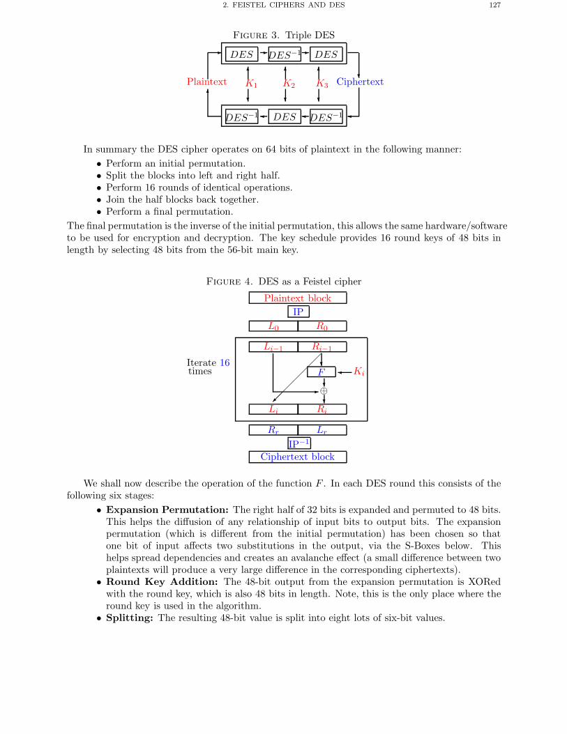
2. FEISTEL CIPHERS AND DES 127
Figure 3. Triple DES
DES−1 DES DES−1� � �
�Plaintext
�K1
�K2
�K3
DES DES−1 DES
Ciphertext
In summary the DES cipher operates on 64 bits of plaintext in the following manner:• Perform an initial permutation.• Split the blocks into left and right half.• Perform 16 rounds of identical operations.• Join the half blocks back together.• Perform a final permutation.
The final permutation is the inverse of the initial permutation, this allows the same hardware/softwareto be used for encryption and decryption. The key schedule provides 16 round keys of 48 bits inlength by selecting 48 bits from the 56-bit main key.
Figure 4. DES as a Feistel cipher
Plaintext blockIP
L0 R0
Iterate 16times
Li−1 Ri−1
��
��
���
F Ki�
⊕
Li Ri
Rr Lr
IP−1
Ciphertext block
We shall now describe the operation of the function F . In each DES round this consists of thefollowing six stages:
• Expansion Permutation: The right half of 32 bits is expanded and permuted to 48 bits.This helps the diffusion of any relationship of input bits to output bits. The expansionpermutation (which is different from the initial permutation) has been chosen so thatone bit of input affects two substitutions in the output, via the S-Boxes below. Thishelps spread dependencies and creates an avalanche effect (a small difference between twoplaintexts will produce a very large difference in the corresponding ciphertexts).
• Round Key Addition: The 48-bit output from the expansion permutation is XORedwith the round key, which is also 48 bits in length. Note, this is the only place where theround key is used in the algorithm.
• Splitting: The resulting 48-bit value is split into eight lots of six-bit values.
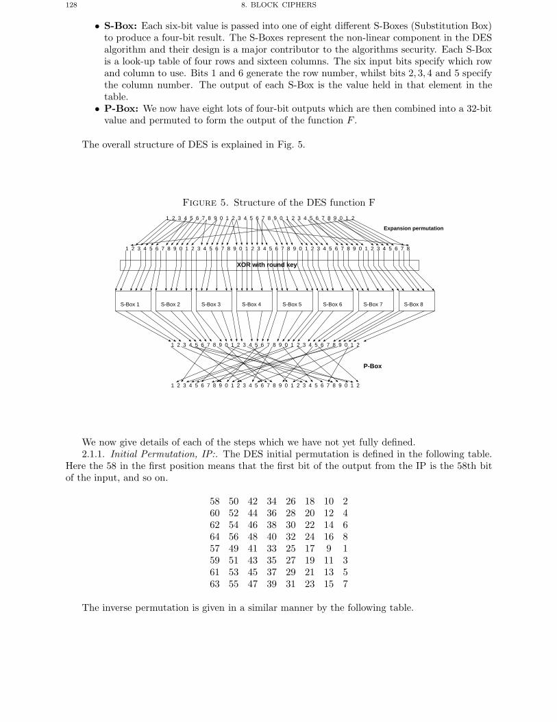
128 8. BLOCK CIPHERS
• S-Box: Each six-bit value is passed into one of eight different S-Boxes (Substitution Box)to produce a four-bit result. The S-Boxes represent the non-linear component in the DESalgorithm and their design is a major contributor to the algorithms security. Each S-Boxis a look-up table of four rows and sixteen columns. The six input bits specify which rowand column to use. Bits 1 and 6 generate the row number, whilst bits 2, 3, 4 and 5 specifythe column number. The output of each S-Box is the value held in that element in thetable.
• P-Box: We now have eight lots of four-bit outputs which are then combined into a 32-bitvalue and permuted to form the output of the function F .
The overall structure of DES is explained in Fig. 5.
Figure 5. Structure of the DES function F1 2 3 4 5 6 7 8 9 0 1 2 3 4 5 6 7 8 9 0 1 2 3 4 5 6 7 8 9 0 1 2
1 2 3 4 5 6 7 8 9 0 1 2 3 4 5 6 7 8 9 0 1 2 3 4 5 6 7 8 9 0 1 2 3 4 5 6 7 8 9 0 1 2 3 4 5 6 7 8
XOR with round key
S-Box 1 S-Box 2 S-Box 3 S-Box 4 S-Box 5 S-Box 6 S-Box 7 S-Box 8
1 2 3 4 5 6 7 8 9 0 1 2 3 4 5 6 7 8 9 0 1 2 3 4 5 6 7 8 9 0 1 2
1 2 3 4 5 6 7 8 9 0 1 2 3 4 5 6 7 8 9 0 1 2 3 4 5 6 7 8 9 0 1 2
P-Box
Expansion permutation
We now give details of each of the steps which we have not yet fully defined.2.1.1. Initial Permutation, IP:. The DES initial permutation is defined in the following table.
Here the 58 in the first position means that the first bit of the output from the IP is the 58th bitof the input, and so on.
58 50 42 34 26 18 10 260 52 44 36 28 20 12 462 54 46 38 30 22 14 664 56 48 40 32 24 16 857 49 41 33 25 17 9 159 51 43 35 27 19 11 361 53 45 37 29 21 13 563 55 47 39 31 23 15 7
The inverse permutation is given in a similar manner by the following table.
2. FEISTEL CIPHERS AND DES 129
40 8 48 16 56 24 64 3239 7 47 15 55 23 63 3138 6 46 14 54 22 62 3037 5 45 13 53 21 61 2936 4 44 12 52 20 60 2835 3 43 11 51 19 59 2734 2 42 10 50 18 58 2633 1 41 9 49 17 57 25
2.1.2. Expansion Permutation, E:. The expansion permutation is given in the following table.Each row corresponds to the bits which are input into the corresponding S-Box at the next stage.Notice how the bits which select a row of one S-Box (the first and last bit on each row) are alsoused to select the column of another S-Box.
32 1 2 3 4 54 5 6 7 8 98 9 10 11 12 1312 13 14 15 16 1716 17 18 19 20 2120 21 22 23 24 2524 25 26 27 28 2928 29 30 31 32 1
2.1.3. S-Box: The details of the eight DES S-Boxes are given in the Fig. 6. Recall that eachbox consists of a table with four rows and sixteen columns.
2.1.4. The P-Box Permutation, P:. The P-Box permutation takes the eight lots of four-bitnibbles, output of the S-Boxes, and produces a 32-bit permutation of these values as given by thefollowing table.
16 7 20 2129 12 28 171 15 23 265 18 31 102 8 24 1432 27 3 919 13 30 622 11 4 25
2.2. DES Key Schedule. The DES key schedule takes the 56-bit key, which is actually inputas a bitstring of 64 bits comprising of the key and eight parity bits, for error detection. These paritybits are in bit positions 8, 16, . . . , 64 and ensure that each byte of the key contains an odd numberof bits.
We first permute the bits of the key according to the following permutation (which takes a64-bit input and produces a 56-bit output, hence discarding the parity bits).
57 49 41 33 25 17 91 58 50 42 34 26 1810 2 59 51 43 35 2719 11 3 60 52 44 3663 55 47 39 31 23 157 62 54 46 38 30 2214 6 61 53 45 37 2921 13 5 28 20 12 4
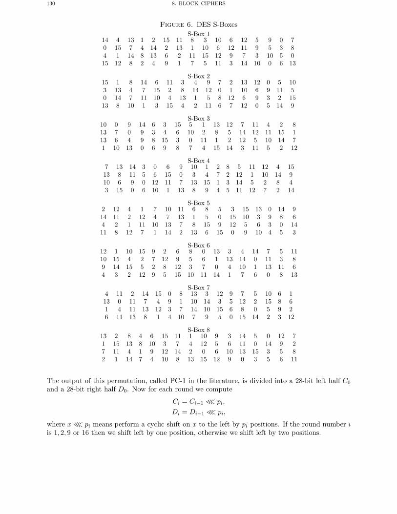
130 8. BLOCK CIPHERS
Figure 6. DES S-BoxesS-Box 1
14 4 13 1 2 15 11 8 3 10 6 12 5 9 0 70 15 7 4 14 2 13 1 10 6 12 11 9 5 3 84 1 14 8 13 6 2 11 15 12 9 7 3 10 5 015 12 8 2 4 9 1 7 5 11 3 14 10 0 6 13
S-Box 215 1 8 14 6 11 3 4 9 7 2 13 12 0 5 103 13 4 7 15 2 8 14 12 0 1 10 6 9 11 50 14 7 11 10 4 13 1 5 8 12 6 9 3 2 1513 8 10 1 3 15 4 2 11 6 7 12 0 5 14 9
S-Box 310 0 9 14 6 3 15 5 1 13 12 7 11 4 2 813 7 0 9 3 4 6 10 2 8 5 14 12 11 15 113 6 4 9 8 15 3 0 11 1 2 12 5 10 14 71 10 13 0 6 9 8 7 4 15 14 3 11 5 2 12
S-Box 47 13 14 3 0 6 9 10 1 2 8 5 11 12 4 1513 8 11 5 6 15 0 3 4 7 2 12 1 10 14 910 6 9 0 12 11 7 13 15 1 3 14 5 2 8 43 15 0 6 10 1 13 8 9 4 5 11 12 7 2 14
S-Box 52 12 4 1 7 10 11 6 8 5 3 15 13 0 14 914 11 2 12 4 7 13 1 5 0 15 10 3 9 8 64 2 1 11 10 13 7 8 15 9 12 5 6 3 0 1411 8 12 7 1 14 2 13 6 15 0 9 10 4 5 3
S-Box 612 1 10 15 9 2 6 8 0 13 3 4 14 7 5 1110 15 4 2 7 12 9 5 6 1 13 14 0 11 3 89 14 15 5 2 8 12 3 7 0 4 10 1 13 11 64 3 2 12 9 5 15 10 11 14 1 7 6 0 8 13
S-Box 74 11 2 14 15 0 8 13 3 12 9 7 5 10 6 113 0 11 7 4 9 1 10 14 3 5 12 2 15 8 61 4 11 13 12 3 7 14 10 15 6 8 0 5 9 26 11 13 8 1 4 10 7 9 5 0 15 14 2 3 12
S-Box 813 2 8 4 6 15 11 1 10 9 3 14 5 0 12 71 15 13 8 10 3 7 4 12 5 6 11 0 14 9 27 11 4 1 9 12 14 2 0 6 10 13 15 3 5 82 1 14 7 4 10 8 13 15 12 9 0 3 5 6 11
The output of this permutation, called PC-1 in the literature, is divided into a 28-bit left half C0
and a 28-bit right half D0. Now for each round we compute
Ci = Ci−1 ≪ pi,
Di = Di−1 ≪ pi,
where x ≪ pi means perform a cyclic shift on x to the left by pi positions. If the round number iis 1, 2, 9 or 16 then we shift left by one position, otherwise we shift left by two positions.
3. RIJNDAEL 131
Finally the two portions Ci and Di are joined back together and are subject to another per-mutation, called PC-2, to produce the final 48-bit round key. The permutation PC-2 is describedbelow.
14 17 11 24 1 53 28 15 6 21 1023 19 12 4 26 816 7 27 20 13 241 52 31 37 47 5530 40 51 45 33 4844 49 39 56 34 5346 42 50 36 29 32
3. Rijndael
The AES winner was decided in fall 2000 to be the Rijndael algorithm designed by Daemenand Rijmen. Rijndael is a block cipher which does not rely on the basic design of the Feistel cipher.However, Rijndael does have a number of similarities with DES. It uses a repeated number of roundsto obtain security and each round consists of substitutions and permutations, plus a key additionphase. Rijndael in addition has a strong mathematical structure, as most of its operations are basedon arithmetic in the field F28 . However, unlike DES the encryption and decryption operations aredistinct.
Recall that elements of F28 are stored as bit vectors (or bytes) representing binary polynomials.For example the byte given by 0x83 in hexadecimal, gives the bit pattern
1, 0, 0, 0, 0, 0, 1, 1
since0x83 = 8 · 16 + 3 = 131
in decimal. One can obtain the bit pattern directly by noticing that 8 in binary is 1, 0, 0, 0 and 3 in4-bit binary is 0, 0, 1, 1 and one simply concatenates these two bit strings together. The bit patternitself then corresponds to the binary polynomial
x7 + x+ 1.
So we say that the hexadecimal number 0x83 represents the binary polynomial
x7 + x+ 1.
Arithmetic in F28 is performed using polynomial arithmetic modulo the irreducible polynomial
m(x) = x8 + x4 + x3 + x+ 1.
Rijndael identifies 32-bit words with polynomials in F28 [X] of degree less than four. This is donein a big-endian format, in that the smallest index corresponds to the least important coefficient.Hence, the word
a0‖a1‖a2‖a3
will correspond to the polynomial
a3X3 + a2X
2 + a1X + a0.
Arithmetic is performed on polynomials in F28[X] modulo the reducible polynomial
M(X) = X4 + 1.
Hence, arithmetic is done on these polynomials in a ring rather than a field, sinceM(X) is reducible.Rijndael is a parametrized algorithm in that it can operate on block sizes of 128, 192 or 256
bits, it can also accept keys of size 128, 192 or 256 bits. For each combination of block and keysize a different number of rounds is specified. To make our discussion simpler we shall consider
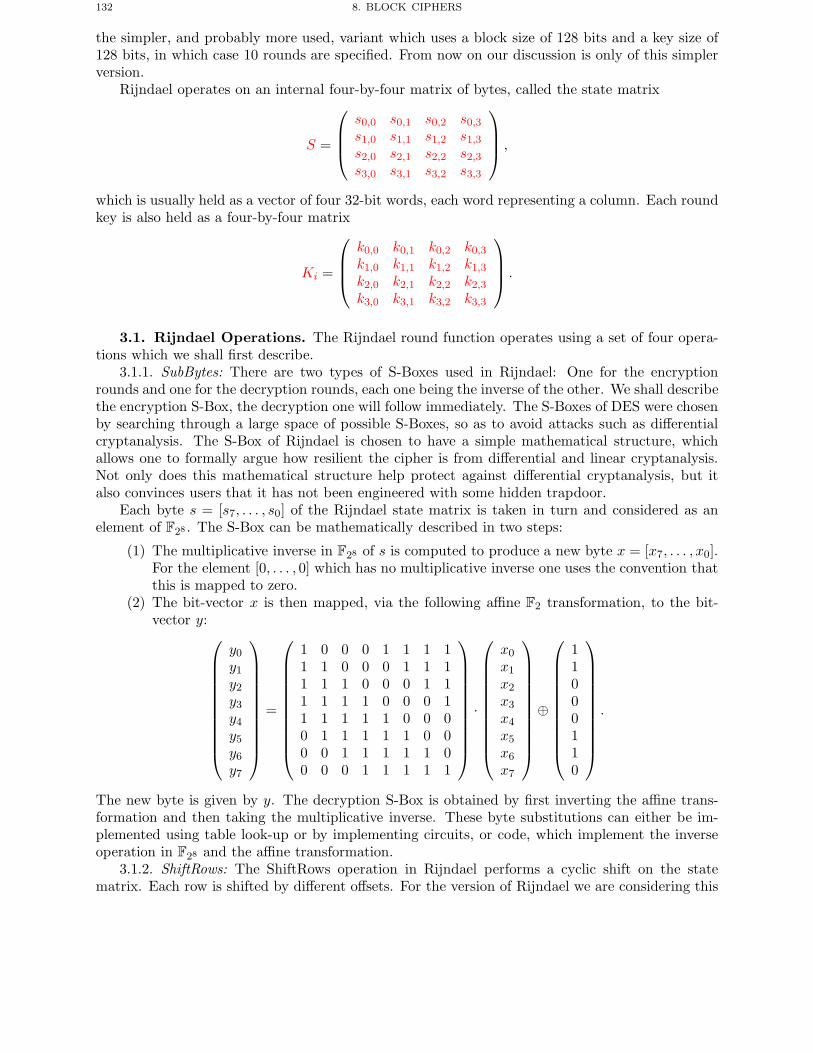
132 8. BLOCK CIPHERS
the simpler, and probably more used, variant which uses a block size of 128 bits and a key size of128 bits, in which case 10 rounds are specified. From now on our discussion is only of this simplerversion.
Rijndael operates on an internal four-by-four matrix of bytes, called the state matrix
S =
⎛⎜⎜⎝
s0,0 s0,1 s0,2 s0,3s1,0 s1,1 s1,2 s1,3s2,0 s2,1 s2,2 s2,3s3,0 s3,1 s3,2 s3,3
⎞⎟⎟⎠ ,
which is usually held as a vector of four 32-bit words, each word representing a column. Each roundkey is also held as a four-by-four matrix
Ki =
⎛⎜⎜⎝
k0,0 k0,1 k0,2 k0,3
k1,0 k1,1 k1,2 k1,3
k2,0 k2,1 k2,2 k2,3
k3,0 k3,1 k3,2 k3,3
⎞⎟⎟⎠ .
3.1. Rijndael Operations. The Rijndael round function operates using a set of four opera-tions which we shall first describe.
3.1.1. SubBytes: There are two types of S-Boxes used in Rijndael: One for the encryptionrounds and one for the decryption rounds, each one being the inverse of the other. We shall describethe encryption S-Box, the decryption one will follow immediately. The S-Boxes of DES were chosenby searching through a large space of possible S-Boxes, so as to avoid attacks such as differentialcryptanalysis. The S-Box of Rijndael is chosen to have a simple mathematical structure, whichallows one to formally argue how resilient the cipher is from differential and linear cryptanalysis.Not only does this mathematical structure help protect against differential cryptanalysis, but italso convinces users that it has not been engineered with some hidden trapdoor.
Each byte s = [s7, . . . , s0] of the Rijndael state matrix is taken in turn and considered as anelement of F28 . The S-Box can be mathematically described in two steps:
(1) The multiplicative inverse in F28 of s is computed to produce a new byte x = [x7, . . . , x0].For the element [0, . . . , 0] which has no multiplicative inverse one uses the convention thatthis is mapped to zero.
(2) The bit-vector x is then mapped, via the following affine F2 transformation, to the bit-vector y:⎛
⎜⎜⎜⎜⎜⎜⎜⎜⎜⎜⎝
y0
y1
y2
y3
y4
y5
y6
y7
⎞⎟⎟⎟⎟⎟⎟⎟⎟⎟⎟⎠
=
⎛⎜⎜⎜⎜⎜⎜⎜⎜⎜⎜⎝
1 0 0 0 1 1 1 11 1 0 0 0 1 1 11 1 1 0 0 0 1 11 1 1 1 0 0 0 11 1 1 1 1 0 0 00 1 1 1 1 1 0 00 0 1 1 1 1 1 00 0 0 1 1 1 1 1
⎞⎟⎟⎟⎟⎟⎟⎟⎟⎟⎟⎠
·
⎛⎜⎜⎜⎜⎜⎜⎜⎜⎜⎜⎝
x0
x1
x2
x3
x4
x5
x6
x7
⎞⎟⎟⎟⎟⎟⎟⎟⎟⎟⎟⎠
⊕
⎛⎜⎜⎜⎜⎜⎜⎜⎜⎜⎜⎝
11000110
⎞⎟⎟⎟⎟⎟⎟⎟⎟⎟⎟⎠.
The new byte is given by y. The decryption S-Box is obtained by first inverting the affine trans-formation and then taking the multiplicative inverse. These byte substitutions can either be im-plemented using table look-up or by implementing circuits, or code, which implement the inverseoperation in F28 and the affine transformation.
3.1.2. ShiftRows: The ShiftRows operation in Rijndael performs a cyclic shift on the statematrix. Each row is shifted by different offsets. For the version of Rijndael we are considering this
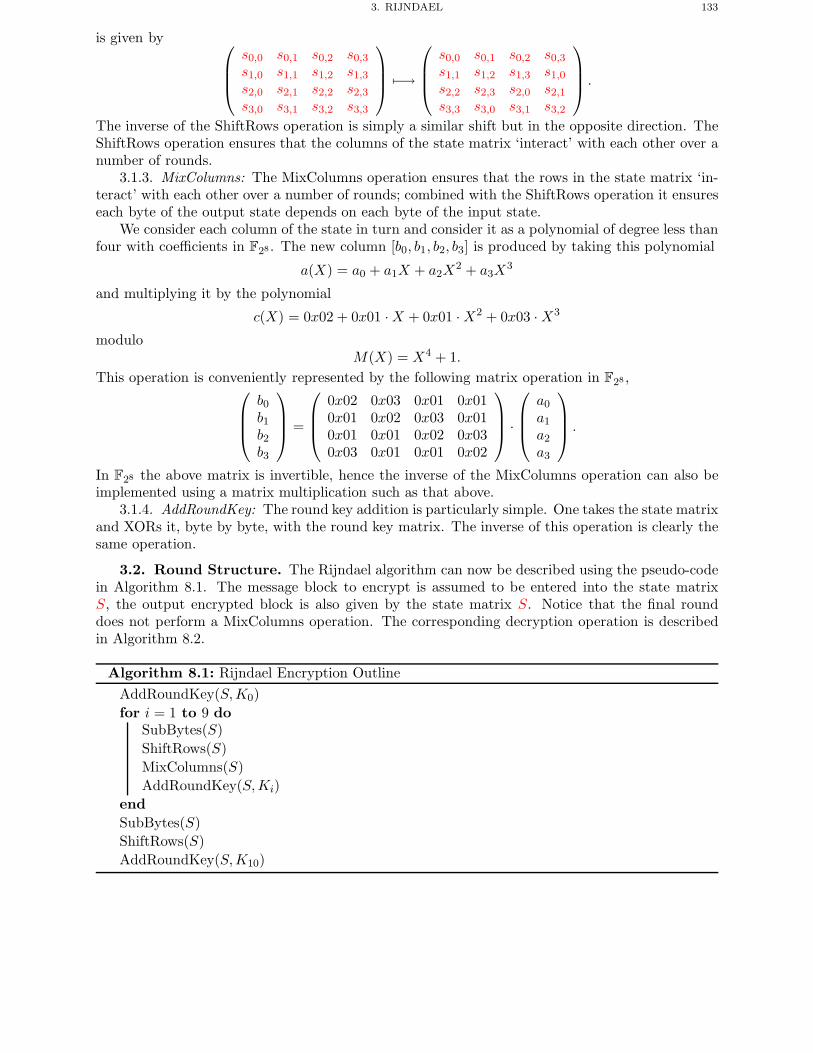
3. RIJNDAEL 133
is given by ⎛⎜⎜⎝
s0,0 s0,1 s0,2 s0,3s1,0 s1,1 s1,2 s1,3s2,0 s2,1 s2,2 s2,3s3,0 s3,1 s3,2 s3,3
⎞⎟⎟⎠ −→
⎛⎜⎜⎝
s0,0 s0,1 s0,2 s0,3s1,1 s1,2 s1,3 s1,0s2,2 s2,3 s2,0 s2,1s3,3 s3,0 s3,1 s3,2
⎞⎟⎟⎠ .
The inverse of the ShiftRows operation is simply a similar shift but in the opposite direction. TheShiftRows operation ensures that the columns of the state matrix ‘interact’ with each other over anumber of rounds.
3.1.3. MixColumns: The MixColumns operation ensures that the rows in the state matrix ‘in-teract’ with each other over a number of rounds; combined with the ShiftRows operation it ensureseach byte of the output state depends on each byte of the input state.
We consider each column of the state in turn and consider it as a polynomial of degree less thanfour with coefficients in F28. The new column [b0, b1, b2, b3] is produced by taking this polynomial
a(X) = a0 + a1X + a2X2 + a3X
3
and multiplying it by the polynomial
c(X) = 0x02 + 0x01 ·X + 0x01 ·X2 + 0x03 ·X3
moduloM(X) = X4 + 1.
This operation is conveniently represented by the following matrix operation in F28 ,⎛⎜⎜⎝
b0b1b2b3
⎞⎟⎟⎠ =
⎛⎜⎜⎝
0x02 0x03 0x01 0x010x01 0x02 0x03 0x010x01 0x01 0x02 0x030x03 0x01 0x01 0x02
⎞⎟⎟⎠ ·
⎛⎜⎜⎝
a0
a1
a2
a3
⎞⎟⎟⎠ .
In F28 the above matrix is invertible, hence the inverse of the MixColumns operation can also beimplemented using a matrix multiplication such as that above.
3.1.4. AddRoundKey: The round key addition is particularly simple. One takes the state matrixand XORs it, byte by byte, with the round key matrix. The inverse of this operation is clearly thesame operation.
3.2. Round Structure. The Rijndael algorithm can now be described using the pseudo-codein Algorithm 8.1. The message block to encrypt is assumed to be entered into the state matrixS, the output encrypted block is also given by the state matrix S. Notice that the final rounddoes not perform a MixColumns operation. The corresponding decryption operation is describedin Algorithm 8.2.
Algorithm 8.1: Rijndael Encryption OutlineAddRoundKey(S,K0)for i = 1 to 9 do
SubBytes(S)ShiftRows(S)MixColumns(S)AddRoundKey(S,Ki)
endSubBytes(S)ShiftRows(S)AddRoundKey(S,K10)
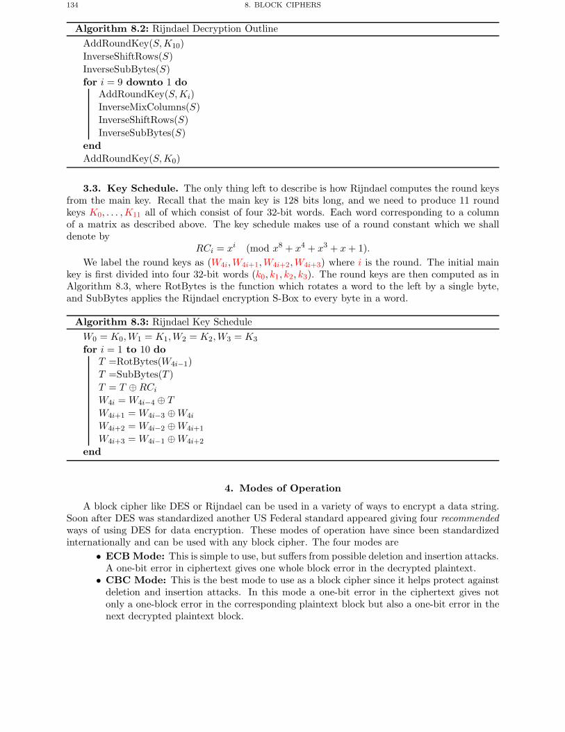
134 8. BLOCK CIPHERS
Algorithm 8.2: Rijndael Decryption OutlineAddRoundKey(S,K10)InverseShiftRows(S)InverseSubBytes(S)for i = 9 downto 1 do
AddRoundKey(S,Ki)InverseMixColumns(S)InverseShiftRows(S)InverseSubBytes(S)
endAddRoundKey(S,K0)
3.3. Key Schedule. The only thing left to describe is how Rijndael computes the round keysfrom the main key. Recall that the main key is 128 bits long, and we need to produce 11 roundkeys K0, . . . ,K11 all of which consist of four 32-bit words. Each word corresponding to a columnof a matrix as described above. The key schedule makes use of a round constant which we shalldenote by
RCi = xi (mod x8 + x4 + x3 + x+ 1).We label the round keys as (W4i,W4i+1,W4i+2,W4i+3) where i is the round. The initial main
key is first divided into four 32-bit words (k0, k1, k2, k3). The round keys are then computed as inAlgorithm 8.3, where RotBytes is the function which rotates a word to the left by a single byte,and SubBytes applies the Rijndael encryption S-Box to every byte in a word.
Algorithm 8.3: Rijndael Key ScheduleW0 = K0,W1 = K1,W2 = K2,W3 = K3
for i = 1 to 10 doT =RotBytes(W4i−1)T =SubBytes(T )T = T ⊕RCiW4i = W4i−4 ⊕ T
W4i+1 = W4i−3 ⊕W4i
W4i+2 = W4i−2 ⊕W4i+1
W4i+3 = W4i−1 ⊕W4i+2
end
4. Modes of Operation
A block cipher like DES or Rijndael can be used in a variety of ways to encrypt a data string.Soon after DES was standardized another US Federal standard appeared giving four recommendedways of using DES for data encryption. These modes of operation have since been standardizedinternationally and can be used with any block cipher. The four modes are
• ECB Mode: This is simple to use, but suffers from possible deletion and insertion attacks.A one-bit error in ciphertext gives one whole block error in the decrypted plaintext.
• CBC Mode: This is the best mode to use as a block cipher since it helps protect againstdeletion and insertion attacks. In this mode a one-bit error in the ciphertext gives notonly a one-block error in the corresponding plaintext block but also a one-bit error in thenext decrypted plaintext block.
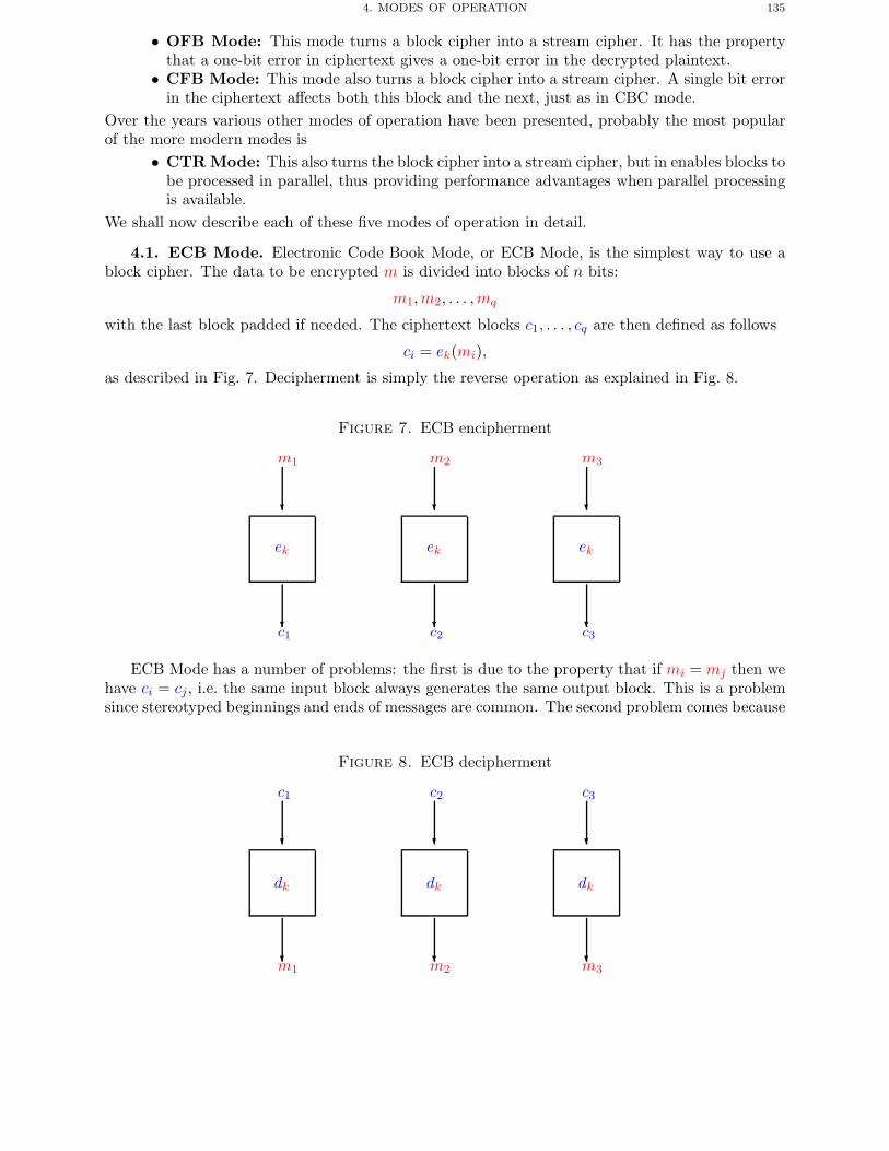
4. MODES OF OPERATION 135
• OFB Mode: This mode turns a block cipher into a stream cipher. It has the propertythat a one-bit error in ciphertext gives a one-bit error in the decrypted plaintext.
• CFB Mode: This mode also turns a block cipher into a stream cipher. A single bit errorin the ciphertext affects both this block and the next, just as in CBC mode.
Over the years various other modes of operation have been presented, probably the most popularof the more modern modes is
• CTR Mode: This also turns the block cipher into a stream cipher, but in enables blocks tobe processed in parallel, thus providing performance advantages when parallel processingis available.
We shall now describe each of these five modes of operation in detail.
4.1. ECB Mode. Electronic Code Book Mode, or ECB Mode, is the simplest way to use ablock cipher. The data to be encrypted m is divided into blocks of n bits:
m1,m2, . . . ,mq
with the last block padded if needed. The ciphertext blocks c1, . . . , cq are then defined as follows
ci = ek(mi),
as described in Fig. 7. Decipherment is simply the reverse operation as explained in Fig. 8.
Figure 7. ECB encipherment
m1
ek
c1
m2
ek
c2
m3
ek
c3
ECB Mode has a number of problems: the first is due to the property that if mi = mj then wehave ci = cj , i.e. the same input block always generates the same output block. This is a problemsince stereotyped beginnings and ends of messages are common. The second problem comes because
Figure 8. ECB decipherment
c1
dk
m1
c2
dk
m2
c3
dk
m3
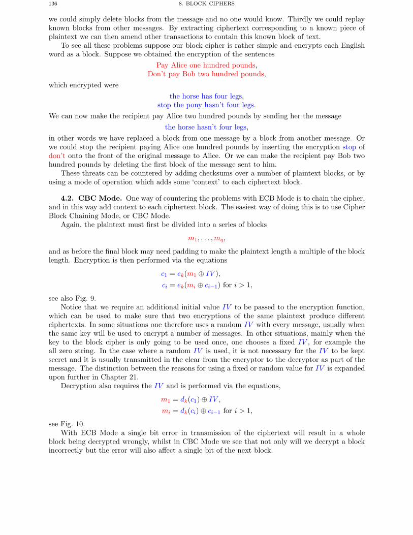
136 8. BLOCK CIPHERS
we could simply delete blocks from the message and no one would know. Thirdly we could replayknown blocks from other messages. By extracting ciphertext corresponding to a known piece ofplaintext we can then amend other transactions to contain this known block of text.
To see all these problems suppose our block cipher is rather simple and encrypts each Englishword as a block. Suppose we obtained the encryption of the sentences
Pay Alice one hundred pounds,Don’t pay Bob two hundred pounds,
which encrypted werethe horse has four legs,
stop the pony hasn’t four legs.We can now make the recipient pay Alice two hundred pounds by sending her the message
the horse hasn’t four legs,in other words we have replaced a block from one message by a block from another message. Orwe could stop the recipient paying Alice one hundred pounds by inserting the encryption stop ofdon’t onto the front of the original message to Alice. Or we can make the recipient pay Bob twohundred pounds by deleting the first block of the message sent to him.
These threats can be countered by adding checksums over a number of plaintext blocks, or byusing a mode of operation which adds some ‘context’ to each ciphertext block.
4.2. CBC Mode. One way of countering the problems with ECB Mode is to chain the cipher,and in this way add context to each ciphertext block. The easiest way of doing this is to use CipherBlock Chaining Mode, or CBC Mode.
Again, the plaintext must first be divided into a series of blocks
m1, . . . ,mq,
and as before the final block may need padding to make the plaintext length a multiple of the blocklength. Encryption is then performed via the equations
c1 = ek(m1 ⊕ IV ),
ci = ek(mi ⊕ ci−1) for i > 1,
see also Fig. 9.Notice that we require an additional initial value IV to be passed to the encryption function,
which can be used to make sure that two encryptions of the same plaintext produce differentciphertexts. In some situations one therefore uses a random IV with every message, usually whenthe same key will be used to encrypt a number of messages. In other situations, mainly when thekey to the block cipher is only going to be used once, one chooses a fixed IV , for example theall zero string. In the case where a random IV is used, it is not necessary for the IV to be keptsecret and it is usually transmitted in the clear from the encryptor to the decryptor as part of themessage. The distinction between the reasons for using a fixed or random value for IV is expandedupon further in Chapter 21.
Decryption also requires the IV and is performed via the equations,
m1 = dk(c1) ⊕ IV ,
mi = dk(ci) ⊕ ci−1 for i > 1,
see Fig. 10.With ECB Mode a single bit error in transmission of the ciphertext will result in a whole
block being decrypted wrongly, whilst in CBC Mode we see that not only will we decrypt a blockincorrectly but the error will also affect a single bit of the next block.
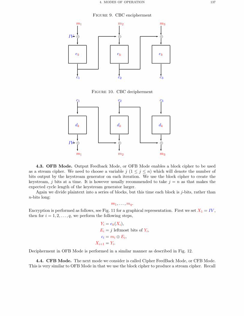
4. MODES OF OPERATION 137
Figure 9. CBC encipherment
IV
m1
⊕
ek
c1
m2
⊕
ek
c2
m3
⊕
ek
c3
Figure 10. CBC decipherment
IV
c1
dk
⊕m1
c2
dk
⊕m2
c3
dk
⊕m3
4.3. OFB Mode. Output Feedback Mode, or OFB Mode enables a block cipher to be usedas a stream cipher. We need to choose a variable j (1 ≤ j ≤ n) which will denote the number ofbits output by the keystream generator on each iteration. We use the block cipher to create thekeystream, j bits at a time. It is however usually recommended to take j = n as that makes theexpected cycle length of the keystream generator larger.
Again we divide plaintext into a series of blocks, but this time each block is j-bits, rather thann-bits long:
m1, . . . ,mq.
Encryption is performed as follows, see Fig. 11 for a graphical representation. First we set X1 = IV ,then for i = 1, 2, . . . , q, we perform the following steps,
Yi = ek(Xi),Ei = j leftmost bits of Yi,ci = mi ⊕ Ei,
Xi+1 = Yi.
Decipherment in OFB Mode is performed in a similar manner as described in Fig. 12.
4.4. CFB Mode. The next mode we consider is called Cipher FeedBack Mode, or CFB Mode.This is very similar to OFB Mode in that we use the block cipher to produce a stream cipher. Recall
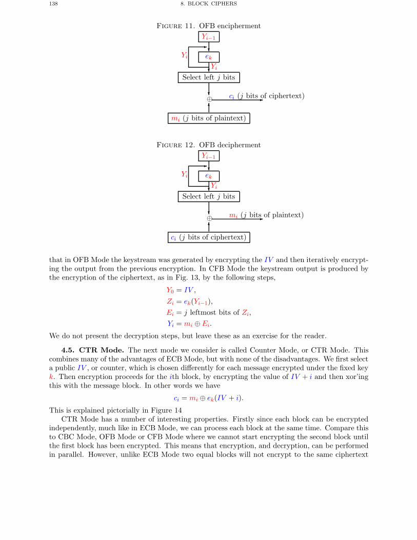
138 8. BLOCK CIPHERS
Figure 11. OFB enciphermentYi−1
ek
Select left j bits
⊕�
mi (j bits of plaintext)
ci (j bits of ciphertext)
Yi
Yi
Figure 12. OFB deciphermentYi−1
ek
Select left j bits
⊕�
ci (j bits of ciphertext)
mi (j bits of plaintext)
Yi
Yi
that in OFB Mode the keystream was generated by encrypting the IV and then iteratively encrypt-ing the output from the previous encryption. In CFB Mode the keystream output is produced bythe encryption of the ciphertext, as in Fig. 13, by the following steps,
Y0 = IV ,
Zi = ek(Yi−1),Ei = j leftmost bits of Zi,Yi = mi ⊕ Ei.
We do not present the decryption steps, but leave these as an exercise for the reader.
4.5. CTR Mode. The next mode we consider is called Counter Mode, or CTR Mode. Thiscombines many of the advantages of ECB Mode, but with none of the disadvantages. We first selecta public IV , or counter, which is chosen differently for each message encrypted under the fixed keyk. Then encryption proceeds for the ith block, by encrypting the value of IV + i and then xor’ingthis with the message block. In other words we have
ci = mi ⊕ ek(IV + i).
This is explained pictorially in Figure 14CTR Mode has a number of interesting properties. Firstly since each block can be encrypted
independently, much like in ECB Mode, we can process each block at the same time. Compare thisto CBC Mode, OFB Mode or CFB Mode where we cannot start encrypting the second block untilthe first block has been encrypted. This means that encryption, and decryption, can be performedin parallel. However, unlike ECB Mode two equal blocks will not encrypt to the same ciphertext
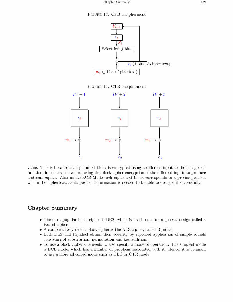
Chapter Summary 139
Figure 13. CFB encipherment
Yi−1
ek
Select left j bits
⊕�
mi (j bits of plaintext)
ci (j bits of ciphertext)
�
Zi
Figure 14. CTR encipherment
IV + 1
ek
⊕m1
c1
IV + 2
ek
⊕m2
c2
IV + 3
ek
⊕m3
c3
value. This is because each plaintext block is encrypted using a different input to the encryptionfunction, in some sense we are using the block cipher encryption of the different inputs to producea stream cipher. Also unlike ECB Mode each ciphertext block corresponds to a precise positionwithin the ciphertext, as its position information is needed to be able to decrypt it successfully.
Chapter Summary
• The most popular block cipher is DES, which is itself based on a general design called aFeistel cipher.
• A comparatively recent block cipher is the AES cipher, called Rijndael.• Both DES and Rijndael obtain their security by repeated application of simple rounds
consisting of substitution, permutation and key addition.• To use a block cipher one needs to also specify a mode of operation. The simplest mode
is ECB mode, which has a number of problems associated with it. Hence, it is commonto use a more advanced mode such as CBC or CTR mode.
140 8. BLOCK CIPHERS
• Some block cipher modes, such as CFB, OFB and CTR modes, allow the block cipher tobe used in a stream cipher.
Further Reading
The Rijndael algorithm, the AES process and a detailed discussion of attacks on block ciphersand Rijndael in particular can be found in the book by Daemen and Rijmen. Stinson’s book is thebest book to explain differential cryptanalysis for students.
J. Daemen and V. Rijmen. The Design of Rijndael: AES – The Advanced Encryption Standard.Springer-Verlag, 2002.
D. Stinson. Cryptography Theory and Practice. CRC Press, 1995.
CHAPTER 9
Symmetric Key Distribution
Chapter Goals
• To understand the problems associated with managing and distributing secret keys.• To learn about key distribution techniques based on symmetric key based protocols.• To introduce the formal analysis of protocols.
1. Key Management
To be able to use symmetric encryption algorithms such as DES or Rijndael we need a way forthe two communicating parties to share the secret key. In this first section we discuss some issuesrelated to how keys are managed, in particular
• key distribution,• key selection,• key lifetime,
But before we continue we need to distinguish between different types of keys. The followingterminology will be used throughout this chapter and beyond:
• Static (or long-term) Keys: These are keys which are to be in use for a long timeperiod. The exact definition of long will depend on the application, but this could meanfrom a few hours to a few years. The compromise of a static key is usually considered tobe a major problem, with potentially catastrophic consequences.
• Ephemeral, or Session (or short-term) Keys: These are keys which have a shortlife-time, maybe a few seconds or a day. They are usually used to provide confidentialityfor the given time period. The compromise of a session key should only result in thecompromise of that session’s secrecy and it should not affect the long-term security of thesystem.
1.1. Key Distribution. Key distribution is one of the fundamental problems with cryptog-raphy. There are a number of solutions to this problem; which one of these one chooses dependson the overall situation.
• Physical Distribution: Using trusted couriers or armed guards, keys can be distributedusing traditional physical means. Until the 1970s this was in effect the only secure way ofdistributing keys at system setup. It has a large number of physical problems associatedwith it, especially scalability, but the main drawback is that security no longer rests withthe key but with the courier. If we can bribe, kidnap or kill the courier then we havebroken the system.
• Distribution Using Symmetric Key Protocols: Once some secret keys have beendistributed between a number of users and a trusted central authority, we can use thetrusted authority to help generate keys for any pair of users as the need arises. Protocolsto perform this task will be discussed in this chapter. They are usually very efficient but
141
142 9. SYMMETRIC KEY DISTRIBUTION
have some drawbacks. In particular they usually assume that both the trusted authorityand the two users who wish to agree on a key are both on-line. They also still require aphysical means to set the initial keys up.
• Distribution Using Public Key Protocols: Using public key cryptography, two par-ties, who have never met or who do not trust any one single authority, can produce ashared secret key. This can be done in an on-line manner, using a key exchange proto-col. Indeed this is the most common application of public key techniques for encryption.Rather than encrypting large amounts of data by public key techniques we agree a key bypublic key techniques and then use a symmetric cipher to actually do the encryption.
To understand the scale of the problem, if our system is to cope with n separate users, andeach user may want to communicate securely with any other user, then we require
n(n− 1)2
separate secret keys. This soon produces huge key management problems; a small university witharound 10 000 students would need to have around fifty million separate secret keys.
With a large number of keys in existence one finds a large number of problems. For examplewhat happens when your key is compromised? In other words someone else has found your key.What can you do about it? What can they do? Hence, a large number of keys produces a largekey management problem.
One solution is for each user to hold only one key with which it communicates with a centralauthority, hence a system with n users will only require n keys. When two users wish to communi-cate they generate a secret key which is only to be used for that message, a so-called session key.This session key can be generated with the help of the central authority using one of the protocolsthat appear later in this chapter.
1.2. Key Selection. The keys which one uses should be truly random, since otherwise anattacker may be able to determine information simply by knowing the more likely keys and themore likely messages, as we saw in a toy example in Chapter 5. All keys should be equally likelyand really need to be generated using a true random number generator, however such a good sourceof entropy is hard to find.
Whilst a truly random key will be very strong, it is hard for a human to remember. Hence,many systems use a password or pass phrase to generate a secret key. But now one needs to worryeven more about brute force attacks. As one can see from the following table, a typical PIN-likepassword of a number between 0 and 9999 is easy to mount a brute force attack against, but evenusing eight printable characters does not push us to the 280 possibilities that we would like to ensuresecurity.
Key size Decimal digits Printable characters4 104 ≈ 213 107 ≈ 223
8 108 ≈ 226 1015 ≈ 250
One solution may be to use long pass phrases of 20–30 characters, but these are likely to lacksufficient entropy since we have already seen that natural language is not very random.
Short passwords based on names or words are a common problem in many large organizations.This is why a number of organizations now have automatic checking that passwords meet certaincriteria such as
• at least one lower case letter,• at least one upper case letter,• at least one numeric character,• at least one non-alpha-numeric character,• at least eight characters in length.
2. SECRET KEY DISTRIBUTION 143
But such rules, even though they eliminate the chance of a dictionary attack, still reduce the numberof possible passwords from what they would be if they were chosen uniformly at random from allchoices of eight printable characters.
1.3. Key Lifetime. One issue one needs to consider when generating and storing keys is thekey lifetime. A general rule is that the longer the key is in use the more vulnerable it will be and themore valuable it will be to an attacker. We have already touched on this when mentioning the use ofsession keys. However, it is important to destroy keys properly after use. Relying on an operatingsystem to delete a file by typing del/rm does not mean that an attacker cannot recover the filecontents by examining the hard disk. Usually deleting a file does not destroy the file contents,it only signals that the file’s location is now available for overwriting with new data. A similarproblem occurs when deleting memory in an application.
1.4. Secret Sharing. As we have mentioned already the main problem is one of managingthe secure distribution of keys. Even a system which uses a trusted central authority needs someway of getting the keys shared between the centre and each user out to the user.
One possible solution is key splitting (more formally called secret sharing) where we divide thekey into a number of shares
K = k1 ⊕ k2 ⊕ · · · ⊕ kr.
Each share is then distributed via separate routes. The beauty of this is that an attacker needs toattack all the routes so as to obtain the key. On the other hand attacking one route will stop thelegitimate user from recovering the key.
We will discuss secret sharing in more detail in Chapter 23.
2. Secret Key Distribution
Recall, if we have n users each of whom wish to communicate securely with each other then wewould require
n(n− 1)2
separate long-term key pairs. As remarked earlier this leads to huge key management problemsand issues related to the distribution of the keys. We have already mentioned that it is better touse session keys and few long-term keys, but we have not explained how one deploys the sessionkeys.
To solve this problem the community developed a number of protocols which make use ofsymmetric key cryptography to distribute secret session keys, some of which we shall describe inthis section. Later on we shall look at public key techniques for this problem, which are often moreelegant.
2.1. Notation. We first need to set up some notation to describe the protocols. Firstly weset up the names of the parties and quantities involved.
• Parties/Principals: A,B, S.Assume the two parties who wish to agree a secret are A and B, for Alice and Bob. Weassume that they will use a trusted third party, or TTP, which we shall denote by S.
• Shared Secret Keys: Kab,Kbs,Kas.Kab will denote a secret key known only to A and B.
• Nonces: Na, Nb.Nonces are numbers used only once, they should be random. The quantity Na will denotea nonce originally produced by the principal A. Note, other notations for nonces arepossible and we will introduce them as the need arises.
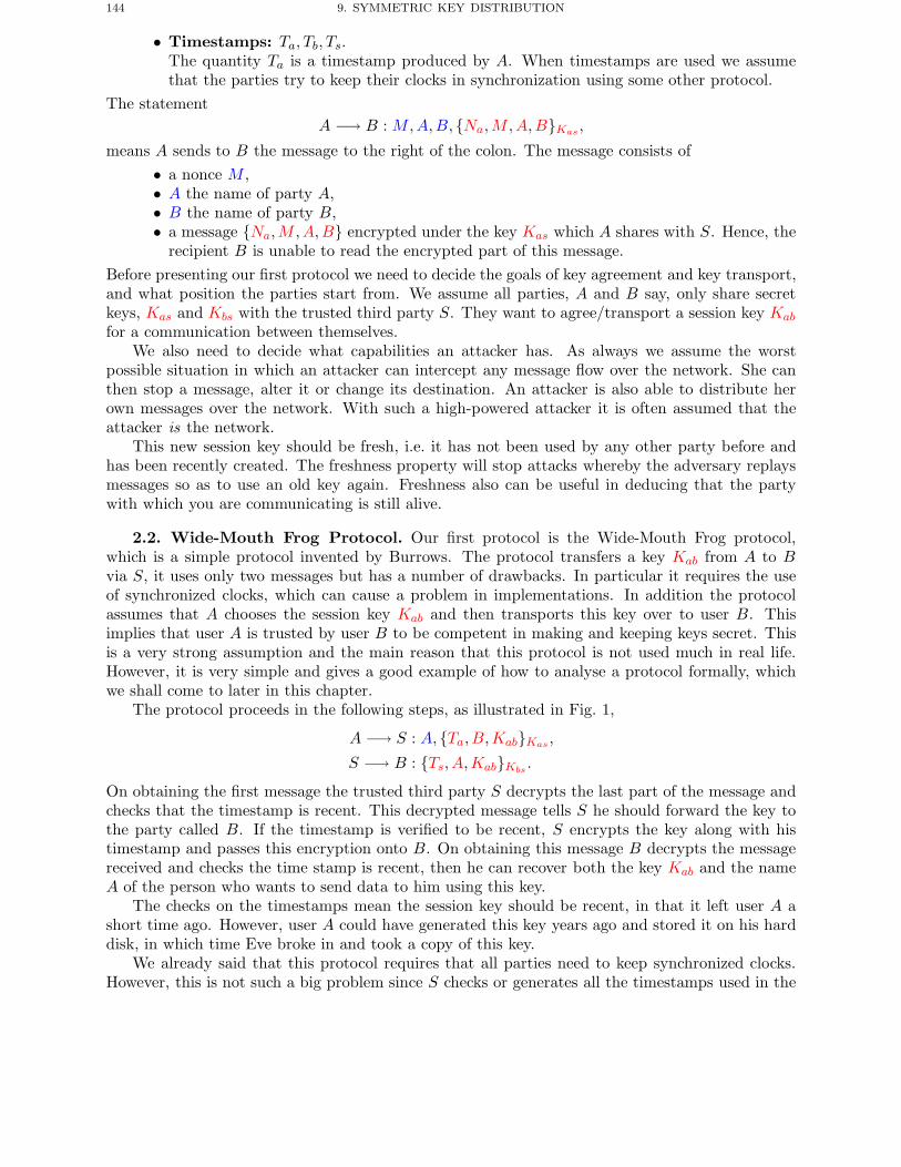
144 9. SYMMETRIC KEY DISTRIBUTION
• Timestamps: Ta, Tb, Ts.The quantity Ta is a timestamp produced by A. When timestamps are used we assumethat the parties try to keep their clocks in synchronization using some other protocol.
The statementA −→ B : M,A,B, {Na,M,A,B}Kas ,
means A sends to B the message to the right of the colon. The message consists of• a nonce M ,• A the name of party A,• B the name of party B,• a message {Na,M,A,B} encrypted under the key Kas which A shares with S. Hence, the
recipient B is unable to read the encrypted part of this message.Before presenting our first protocol we need to decide the goals of key agreement and key transport,and what position the parties start from. We assume all parties, A and B say, only share secretkeys, Kas and Kbs with the trusted third party S. They want to agree/transport a session key Kab
for a communication between themselves.We also need to decide what capabilities an attacker has. As always we assume the worst
possible situation in which an attacker can intercept any message flow over the network. She canthen stop a message, alter it or change its destination. An attacker is also able to distribute herown messages over the network. With such a high-powered attacker it is often assumed that theattacker is the network.
This new session key should be fresh, i.e. it has not been used by any other party before andhas been recently created. The freshness property will stop attacks whereby the adversary replaysmessages so as to use an old key again. Freshness also can be useful in deducing that the partywith which you are communicating is still alive.
2.2. Wide-Mouth Frog Protocol. Our first protocol is the Wide-Mouth Frog protocol,which is a simple protocol invented by Burrows. The protocol transfers a key Kab from A to Bvia S, it uses only two messages but has a number of drawbacks. In particular it requires the useof synchronized clocks, which can cause a problem in implementations. In addition the protocolassumes that A chooses the session key Kab and then transports this key over to user B. Thisimplies that user A is trusted by user B to be competent in making and keeping keys secret. Thisis a very strong assumption and the main reason that this protocol is not used much in real life.However, it is very simple and gives a good example of how to analyse a protocol formally, whichwe shall come to later in this chapter.
The protocol proceeds in the following steps, as illustrated in Fig. 1,
A −→ S : A, {Ta, B,Kab}Kas ,S −→ B : {Ts, A,Kab}Kbs .
On obtaining the first message the trusted third party S decrypts the last part of the message andchecks that the timestamp is recent. This decrypted message tells S he should forward the key tothe party called B. If the timestamp is verified to be recent, S encrypts the key along with histimestamp and passes this encryption onto B. On obtaining this message B decrypts the messagereceived and checks the time stamp is recent, then he can recover both the key Kab and the nameA of the person who wants to send data to him using this key.
The checks on the timestamps mean the session key should be recent, in that it left user A ashort time ago. However, user A could have generated this key years ago and stored it on his harddisk, in which time Eve broke in and took a copy of this key.
We already said that this protocol requires that all parties need to keep synchronized clocks.However, this is not such a big problem since S checks or generates all the timestamps used in the
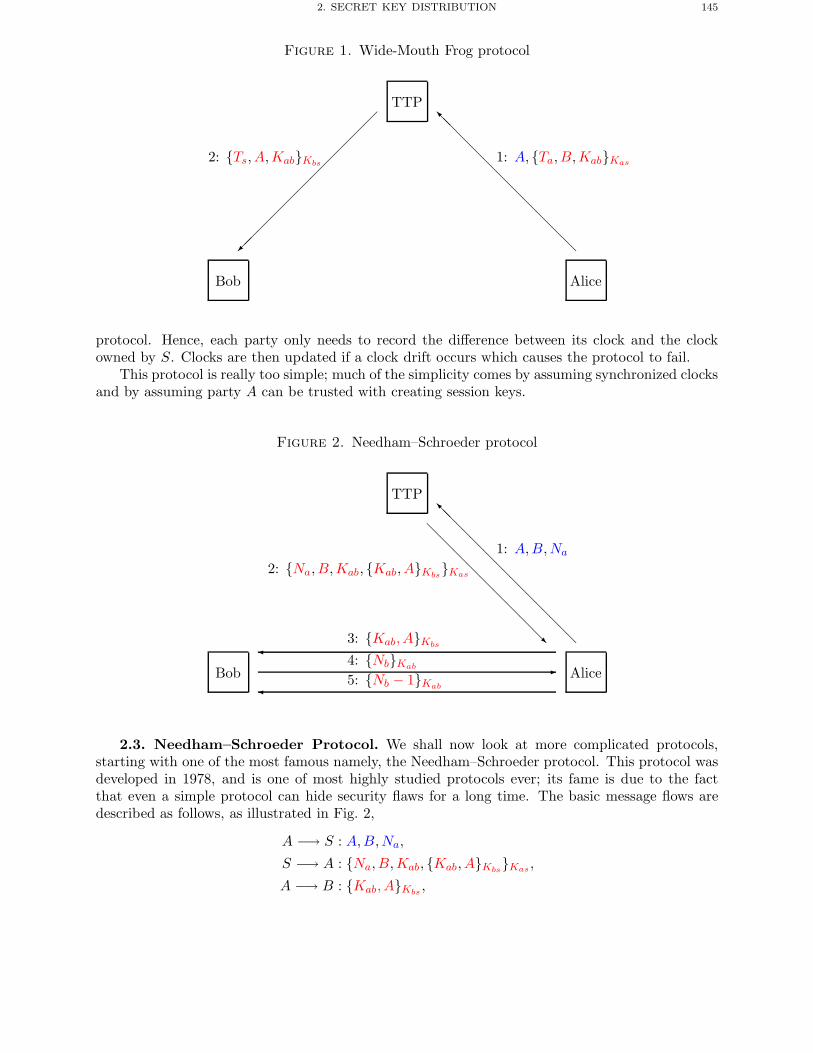
2. SECRET KEY DISTRIBUTION 145
Figure 1. Wide-Mouth Frog protocol
Bob Alice
TTP
�
1: A, {Ta, B,Kab}Kas
��
��
��
��
����
2: {Ts, A,Kab}Kbs
protocol. Hence, each party only needs to record the difference between its clock and the clockowned by S. Clocks are then updated if a clock drift occurs which causes the protocol to fail.
This protocol is really too simple; much of the simplicity comes by assuming synchronized clocksand by assuming party A can be trusted with creating session keys.
Figure 2. Needham–Schroeder protocol
Bob Alice
TTP
�
1: A,B,Na
�
2: {Na, B,Kab, {Kab, A}Kbs}Kas
�3: {Kab, A}Kbs
4: {Nb}Kab
�5: {Nb − 1}Kab
2.3. Needham–Schroeder Protocol. We shall now look at more complicated protocols,starting with one of the most famous namely, the Needham–Schroeder protocol. This protocol wasdeveloped in 1978, and is one of most highly studied protocols ever; its fame is due to the factthat even a simple protocol can hide security flaws for a long time. The basic message flows aredescribed as follows, as illustrated in Fig. 2,
A −→ S : A,B,Na,
S −→ A : {Na, B,Kab, {Kab, A}Kbs}Kas ,A −→ B : {Kab, A}Kbs ,
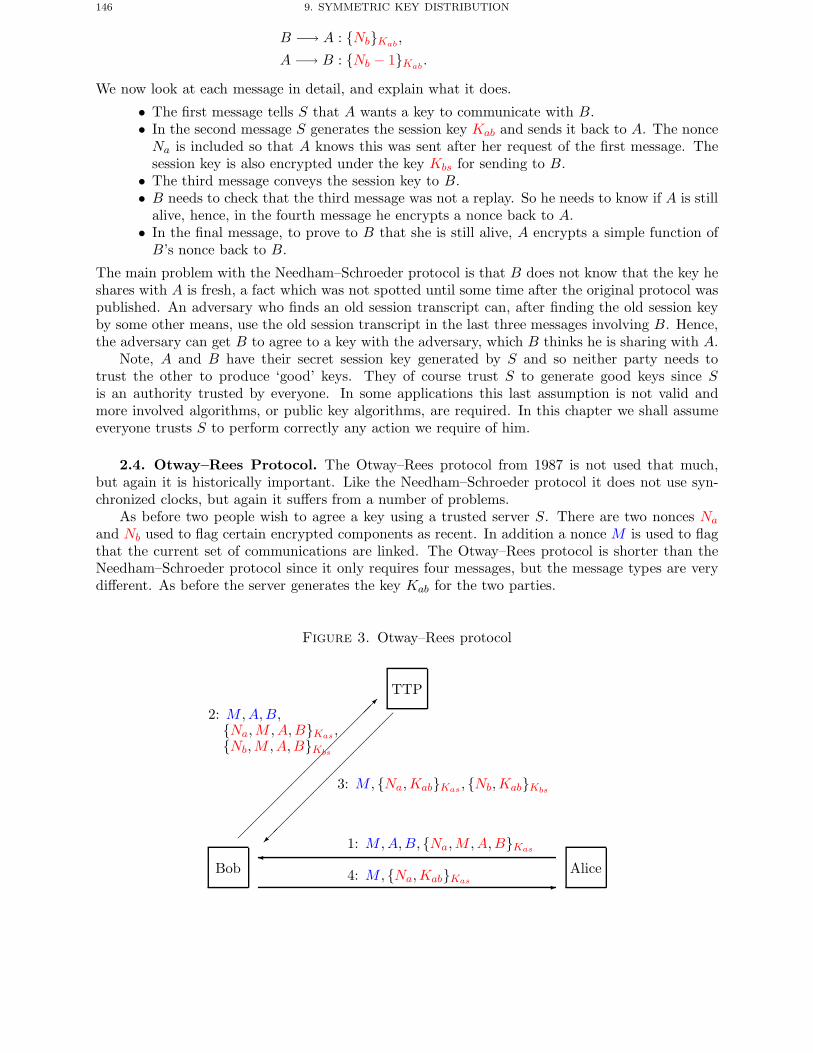
146 9. SYMMETRIC KEY DISTRIBUTION
B −→ A : {Nb}Kab ,A −→ B : {Nb − 1}Kab .
We now look at each message in detail, and explain what it does.
• The first message tells S that A wants a key to communicate with B.• In the second message S generates the session key Kab and sends it back to A. The nonceNa is included so that A knows this was sent after her request of the first message. Thesession key is also encrypted under the key Kbs for sending to B.
• The third message conveys the session key to B.• B needs to check that the third message was not a replay. So he needs to know if A is still
alive, hence, in the fourth message he encrypts a nonce back to A.• In the final message, to prove to B that she is still alive, A encrypts a simple function ofB’s nonce back to B.
The main problem with the Needham–Schroeder protocol is that B does not know that the key heshares with A is fresh, a fact which was not spotted until some time after the original protocol waspublished. An adversary who finds an old session transcript can, after finding the old session keyby some other means, use the old session transcript in the last three messages involving B. Hence,the adversary can get B to agree to a key with the adversary, which B thinks he is sharing with A.
Note, A and B have their secret session key generated by S and so neither party needs totrust the other to produce ‘good’ keys. They of course trust S to generate good keys since Sis an authority trusted by everyone. In some applications this last assumption is not valid andmore involved algorithms, or public key algorithms, are required. In this chapter we shall assumeeveryone trusts S to perform correctly any action we require of him.
2.4. Otway–Rees Protocol. The Otway–Rees protocol from 1987 is not used that much,but again it is historically important. Like the Needham–Schroeder protocol it does not use syn-chronized clocks, but again it suffers from a number of problems.
As before two people wish to agree a key using a trusted server S. There are two nonces Na
and Nb used to flag certain encrypted components as recent. In addition a nonce M is used to flagthat the current set of communications are linked. The Otway–Rees protocol is shorter than theNeedham–Schroeder protocol since it only requires four messages, but the message types are verydifferent. As before the server generates the key Kab for the two parties.
Figure 3. Otway–Rees protocol
Bob Alice
TTP
�1: M,A,B, {Na,M,A,B}Kas
��
��
��
��
����2: M,A,B,
{Na,M,A,B}Kas ,{Nb,M,A,B}Kbs�
��
��
��
��
��
3: M, {Na,Kab}Kas , {Nb,Kab}Kbs
4: M, {Na,Kab}Kas
2. SECRET KEY DISTRIBUTION 147
The message flows in the Otway–Rees protocol are as follows, as illustrated in Fig. 3,
A −→ B : M,A,B, {Na,M,A,B}Kas ,B −→ S : M,A,B, {Na,M,A,B}Kas , {Nb,M,A,B}Kbs ,S −→ B : M, {Na,Kab}Kas , {Nb,Kab}Kbs ,B −→ A : M, {Na,Kab}Kas .
Since the protocol does not make use of Kab as an encryption key, neither party knows whetherthe key is known to each other. We say that Otway–Rees is a protocol which does not offer keyconfirmation. Let us see what the parties do know: A knows that B sent a message containing anonce Na which A knows to be fresh, since A originally generated the nonce. So B must have senta message recently. On the other hand B has been told by the server that A used a nonce, but Bhas no idea whether this was a replay of an old message.
2.5. Kerberos. We end this section by looking at Kerberos. Kerberos is an authenticationsystem based on symmetric encryption with keys shared with an authentication server; it is basedon ideas underlying the Needham–Schroeder protocol. Kerberos was developed at MIT around1987 as part of Project Athena. A modified version of this original version of Kerberos is now usedin Windows 2000.
The network is assumed to consist of clients and a server, where the clients may be users,programs or services. Kerberos keeps a central database of clients including a secret key for eachclient, hence Kerberos requires a key space of size O(n) if we have n clients. Kerberos is used toprovide authentication of one entity to another and to issue session keys to these entities.
In addition Kerberos can run a ticket granting system to enable access control to services andresources. The division between authentication and access is a good idea which we shall see laterechoed in SPKI. This division mirrors what happens in real companies. For example, in a companythe personnel department administers who you are, whilst the computer department administerswhat resources you can use. This division is also echoed in Kerberos with an authentication serverand a ticket generation server TGS. The TGS gives tickets to enable users to access resources, suchas files, printers, etc.
Suppose A wishes to access a resource B. First A logs onto the authentication server using apassword. The user A is given a ticket from this server encrypted under her password. This ticketcontains a session key Kas. She now uses Kas to obtain a ticket from the TGS S to access theresource B. The output of the TGS is a key Kab , a timestamp TS and a lifetime L. The outputof the TGS is used to authenticate A in subsequent traffic with B.
The flows look something like those given in Fig. 4,
A −→ S : A,B,
S −→ A : {TS , L,Kab, B, {TS , L,Kab, A}Kbs}Kas ,A −→ B : {TS , L,Kab, A}Kbs , {A,TA}Kab ,B −→ A : {TA + 1}Kab .
• The first message is A telling S that she wants to access B.• If S allows this access then a ticket {TS , L,Kab, A} is created. This is encrypted underKbs and sent to A for forwarding to B. The user A also gets a copy of the key in a formreadable by her.
• The user A wants to verify that the ticket is valid and that the resource B is alive. Hence,she sends an encrypted nonce/timestamp TA to B.
• The resource B sends back the encryption of TA + 1, after checking that the timestampTA is recent, thus proving he knows the key and is alive.
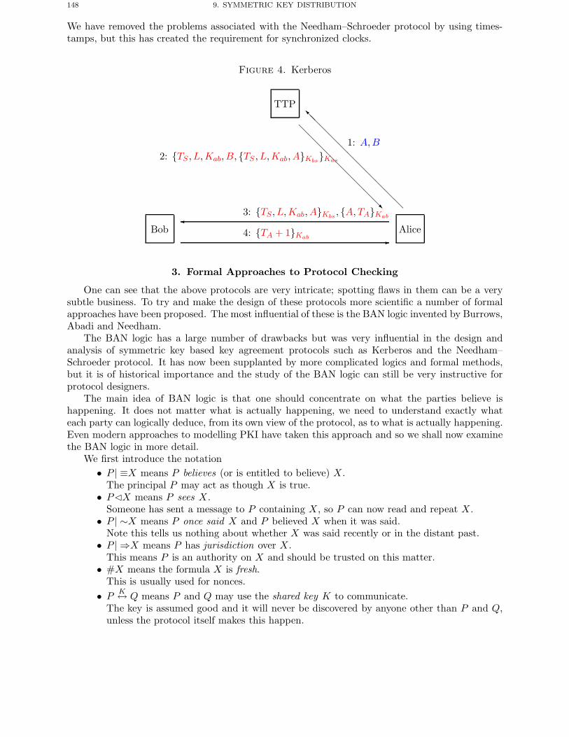
148 9. SYMMETRIC KEY DISTRIBUTION
We have removed the problems associated with the Needham–Schroeder protocol by using times-tamps, but this has created the requirement for synchronized clocks.
Figure 4. Kerberos
Bob Alice
TTP
�
1: A,B
�
2: {TS , L,Kab, B, {TS , L,Kab, A}Kbs}Kas
�3: {TS , L,Kab, A}Kbs , {A,TA}Kab
4: {TA + 1}Kab
3. Formal Approaches to Protocol Checking
One can see that the above protocols are very intricate; spotting flaws in them can be a verysubtle business. To try and make the design of these protocols more scientific a number of formalapproaches have been proposed. The most influential of these is the BAN logic invented by Burrows,Abadi and Needham.
The BAN logic has a large number of drawbacks but was very influential in the design andanalysis of symmetric key based key agreement protocols such as Kerberos and the Needham–Schroeder protocol. It has now been supplanted by more complicated logics and formal methods,but it is of historical importance and the study of the BAN logic can still be very instructive forprotocol designers.
The main idea of BAN logic is that one should concentrate on what the parties believe ishappening. It does not matter what is actually happening, we need to understand exactly whateach party can logically deduce, from its own view of the protocol, as to what is actually happening.Even modern approaches to modelling PKI have taken this approach and so we shall now examinethe BAN logic in more detail.
We first introduce the notation• P | ≡X means P believes (or is entitled to believe) X.
The principal P may act as though X is true.• P�X means P sees X.
Someone has sent a message to P containing X, so P can now read and repeat X.• P | ∼X means P once said X and P believed X when it was said.
Note this tells us nothing about whether X was said recently or in the distant past.• P | ⇒X means P has jurisdiction over X.
This means P is an authority on X and should be trusted on this matter.• #X means the formula X is fresh.
This is usually used for nonces.• P
K↔ Q means P and Q may use the shared key K to communicate.The key is assumed good and it will never be discovered by anyone other than P and Q,unless the protocol itself makes this happen.
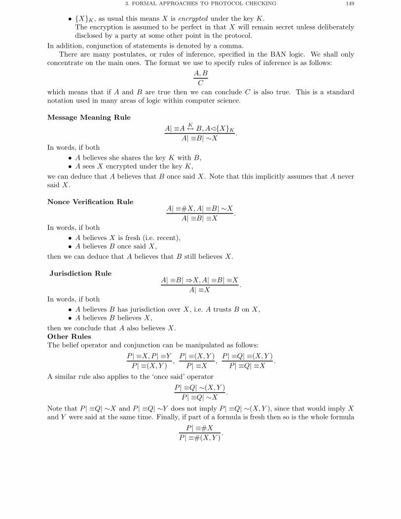
3. FORMAL APPROACHES TO PROTOCOL CHECKING 149
• {X}K , as usual this means X is encrypted under the key K.The encryption is assumed to be perfect in that X will remain secret unless deliberatelydisclosed by a party at some other point in the protocol.
In addition, conjunction of statements is denoted by a comma.There are many postulates, or rules of inference, specified in the BAN logic. We shall only
concentrate on the main ones. The format we use to specify rules of inference is as follows:A,B
C
which means that if A and B are true then we can conclude C is also true. This is a standardnotation used in many areas of logic within computer science.
Message Meaning Rule
A| ≡A K↔ B,A�{X}KA| ≡B| ∼X .
In words, if both• A believes she shares the key K with B,• A sees X encrypted under the key K,
we can deduce that A believes that B once said X. Note that this implicitly assumes that A neversaid X.
Nonce Verification RuleA| ≡#X,A| ≡B| ∼X
A| ≡B| ≡X .
In words, if both• A believes X is fresh (i.e. recent),• A believes B once said X,
then we can deduce that A believes that B still believes X.
Jurisdiction RuleA| ≡B| ⇒X,A| ≡B| ≡X
A| ≡X .
In words, if both• A believes B has jurisdiction over X, i.e. A trusts B on X,• A believes B believes X,
then we conclude that A also believes X.Other RulesThe belief operator and conjunction can be manipulated as follows:
P | ≡X,P | ≡YP | ≡(X,Y )
,P | ≡(X,Y )P | ≡X ,
P | ≡Q| ≡(X,Y )P | ≡Q| ≡X .
A similar rule also applies to the ‘once said’ operatorP | ≡Q| ∼(X,Y )P | ≡Q| ∼X .
Note that P | ≡Q| ∼X and P | ≡Q| ∼Y does not imply P | ≡Q| ∼(X,Y ), since that would imply Xand Y were said at the same time. Finally, if part of a formula is fresh then so is the whole formula
P | ≡#XP | ≡#(X,Y )
.
150 9. SYMMETRIC KEY DISTRIBUTION
We wish to analyse a key agreement protocol between A and B using the BAN logic. But whatis the goal of such a protocol? The minimum we want to achieve is
A| ≡A K↔ B and B| ≡A K↔ B,
i.e. both parties believe they share a secret key with each other.However, we could expect to achieve more, for example
A| ≡B| ≡A K↔ B and B| ≡A| ≡A K↔ B,
which is called key confirmation. In words, we may want to achieve that, after the protocol hasrun, A is assured that B knows he is sharing a key with A, and it is the same key A believes sheis sharing with B.
Before analysing a protocol using the BAN logic we convert the protocol into logical statements.This process is called idealization, and is the most error prone part of the procedure since it cannotbe automated. We also need to specify the assumptions, or axioms, which hold at the beginningof the protocol.
To see this in ‘real life’ we analyse the Wide-Mouth Frog protocol for key agreement usingsynchronized clocks.
3.1. Wide-Mouth Frog Protocol. Recall the Wide-Mouth Frog protocol
A −→ S : A, {Ta, B,Kab}Kas ,S −→ B : {Ts, A,Kab}Kbs .
This becomes the idealized protocol
A −→ S : {Ta, A Kab↔ B}Kas ,S −→ B : {Ts, A| ≡A Kab↔ B}Kbs .
One should read the idealization of the first message as telling S that• Ta is a timestamp/nonce,• Kab is a key which is meant as a key to communicate with B.
So what assumptions exist at the start of the protocol? Clearly A, B and S share secret keys whichin BAN logic becomes
A| ≡A Kas↔ S, S| ≡A Kas↔ S,
B| ≡B Kbs↔ S, S| ≡B Kbs↔ S.There are a couple of nonce assumptions,
S| ≡#Ta and B| ≡#Ts.
Finally, we have the following three assumptions• B trusts A to invent good keys,
B| ≡(A| ⇒AKab↔ B),
• B trusts S to relay the key from A,
B| ≡(S| ⇒A| ≡A Kab↔ B),
• A knows the session key in advance,
A| ≡A Kab↔ B.
Chapter Summary 151
Notice how these last three assumptions specify the problems we associated with this protocol inthe earlier section.
Using these assumptions we can now analyse the protocol. Let us see what we can deduce fromthe first message
A −→ S : {Ta, A Kab↔ B}Kas .• Since S sees the message encrypted under Kas he can deduce that A said the message.• Since Ta is believed by S to be fresh he concludes the whole message is fresh.• Since the whole message is fresh, S concludes that A currently believes the whole of it.• S then concludes
S| ≡A| ≡A Kab↔ B,
which is what we need to conclude so that S can send the second message of the protocol.We now look at what happens when we analyse the second message
S −→ B : {Ts, A| ≡A Kab↔ B}Kbs .• Since B sees the message encrypted under Kbs he can deduce that S said the message.• Since Ts is believed by B to be fresh he concludes the whole message is fresh.• Since the whole message is fresh, B concludes that S currently believes the whole of it.• So B believes that S believes the second part of the message.• But B believes S has authority on whether A knows the key and B believes A has authority
to generate the key.So we conclude
B| ≡A Kab↔ B
andB| ≡A| ≡A Kab↔ B.
Combining with our axiom A| ≡A Kab↔ B we conclude that the key agreement protocol is sound.The only requirement we have not met is that
A| ≡B| ≡A Kab↔ B,
i.e. A does not achieve confirmation that B has received the key.Notice what the application of the BAN logic has done is to make the axioms clearer, so it is
easier to compare which assumptions each protocol needs to make it work. In addition it clarifieswhat the result of running the protocol is from all parties’ points of view.
Chapter Summary
• Distributing secret keys used for symmetric ciphers can be a major problem.• A number of key agreement protocols exist based on a trusted third party and symmet-
ric encryption algorithms. These protocols require long-term keys to have been alreadyestablished with the TTP, they may also require some form of clock synchronization.
• Various logics exist to analyse such protocols. The most influential of these has been theBAN logic. These logics help to identify explicit assumptions and problems associatedwith each protocol.
152 9. SYMMETRIC KEY DISTRIBUTION
Further Reading
The paper by Burrows, Abadi and Needham is a very readable introduction to the BAN logicand a number of key agreement protocols, much of our treatment is based on this paper. Foranother, more modern, approach to protocol checking see the book by Ryan et. al., this covers anapproach based on the CSP process algebra.
M. Burrows, M. Abadi and R. Needham. A Logic of Authentication. Digital Equipment Corpora-tion, SRC Research Report 39, 1990.
P. Ryan, S. Schneider, M. Goldsmith, G. Lowe and B. Ruscoe. Modelling and analysis of securityprotocols. Addison–Wesley, 2001.
CHAPTER 10
Hash Functions and Message Authentication Codes
Chapter Goals
• To understand the properties of cryptographic hash functions.• To understand how existing deployed hash functions work.• To examine the workings of message authentication codes.
1. Introduction
In many situations we do not wish to protect the confidentiality of information, we simplywish to ensure the integrity of information. That is we want to guarantee that data has not beentampered with. In this chapter we look at two mechanisms for this, the first using cryptographichash functions is for when we want to guarantee integrity of information after the application of thefunction. A cryptographic hash function is usually used as a component of another scheme, sincethe integrity is not bound to any entity. The other mechanism we look at is the use of a messageauthentication code. These act like a keyed version of a hash function, they are a symmetric keytechnique which enables the holders of a symmetric key to agree that only they could have producedthe authentication code on a given message.
Hash functions can also be considered as a special type of manipulation detection code, orMDC. For example a hash function can be used to protect the integrity of a large file, as used insome virus protection products. The hash value of the file contents is computed and then eitherstored in a secure place (e.g. on a floppy in a safe) or the hash value is put in a file of similar valueswhich is then digitally signed to stop future tampering.
Both hash functions and MACs will be used extensively later in other schemes. In particularcryptographic hash functions will be used to compress large messages down to smaller ones toenable efficient digital signature algorithms. Another use of hash functions is to produce, in adeterministic manner, random data from given values. We shall see this application when we buildelaborate and “provably secure” encryption schemes later on in the book.
2. Hash Functions
A cryptographic hash function h is a function which takes arbitrary length bit strings as inputand produces a fixed length bit string as output, the output is often called a hashcode or hash value.Hash functions are used a lot in computer science, but the crucial difference between a standardhash function and a cryptographic hash function is that a cryptographic hash function should atleast have the property of being one-way. In other words given any string y from the range of h, itshould be computationally infeasible to find any value x in the domain of h such that
h(x) = y.
Another way to describe a hash function which has the one-way property is that it is preimageresistant. Given a hash function which produces outputs of n bits, we would like a function forwhich finding preimages requires O(2n) time.
153
154 10. HASH FUNCTIONS AND MESSAGE AUTHENTICATION CODES
In practice we need something more than the one-way property. A hash function is calledcollision resistant if it is infeasible to find two distinct values x and x′ such that
h(x) = h(x′).
It is harder to construct collision resistant hash functions than one-way hash functions due to thebirthday paradox. To find a collision of a hash function f , we can keep computing
f(x1), f(x2), f(x3), . . .
until we get a collision. If the function has an output size of n bits then we expect to find acollision after O(2n/2) iterations. This should be compared with the number of steps needed to finda preimage, which should be O(2n) for a well-designed hash function. Hence to achieve a securitylevel of 80 bits for a collision resistant hash function we need roughly 160 bits of output.
But still that is not enough; a cryptographic hash function should also be second preimageresistant. This is the property that given m it should be hard to find anm′ �= m with h(m′) = h(m).Whilst this may look like collision resistance, it is actually related more to preimage resistance. Inparticular a cryptographic hash function with n-bit outputs should require O(2n) operations beforeone can find a second preimage.
In summary a cryptographic hash function needs to satisfy the following three properties:(1) Preimage Resistant: It should be hard to find a message with a given hash value.(2) Collision Resistant: It should be hard to find two messages with the same hash value.(3) Second Preimage Resistant: Given one message it should be hard to find another
message with the same hash value.But how are these properties related. We can relate these properties using reductions.
Lemma 10.1. Assuming a function is preimage resistant for every element of the range of h isa weaker assumption than assuming it either collision resistant or second preimage resistant.
Proof. Suppose h is a function and let O denote an oracle which on input of y finds an x suchthat h(x) = y, i.e. O is an oracle which breaks the preimage resistance of the function h.
Using O we can then find a collision in h by pulling x at random and then computing y = h(x).Passing y to the oracle O will produce a value x′ such that y = h(x′). Since h is assumed to haveinfinite domain, it is unlikely that we have x = x′. Hence, we have found a collision in h.
A similar argument applies to breaking the second preimage resistance of h. �
However, one can construct hash functions which are collision resistant but are not one-wayfor some of the range of h. As an example, let g(x) denote a collision resistant hash function withoutputs of bit length n. Now define a new hash function h(x) with output size n+1 bits as follows:
h(x) ={
0‖x If |x| = n,1‖g(x) Otherwise.
The function h(x) is clearly collision resistant, as we have assumed g(x) is collision resistant. Butthe function h(x) is not preimage resistant as one can invert it on any value in the range whichstarts with a zero bit. So even though we can invert the function h(x) on some of its input we areunable to find collisions.
Lemma 10.2. Assuming a function is second preimage resistant is a weaker assumption thanassuming it is collision resistant.
Proof. Assume we are given an oracle O which on input of x will find x′ such that x �= x′ andh(x) = h(x′). We can clearly use O to find a collision in h by choosing x at random. �
3. DESIGNING HASH FUNCTIONS 155
3. Designing Hash Functions
To be effectively collision free a hash value should be at least 128 bits long, for applications withlow security, but preferably its output should be 160 bits long. However, the input size should bebit strings of (virtually) infinite length. In practice designing functions of infinite domain is hard,hence usually one builds a so called compression function which maps bits strings of length s intobit strings of length n, for s > n, and then chains this in some way so as to produce a function onan infinite domain. We have seen such a situation before when we considered modes of operationof block ciphers.
We first discuss the most famous chaining method, namely the Merkle–Damgard construction,and then we go on to discuss designs for the compression function.
3.1. Merkle–Damgard Construction. Suppose f is a compression function from s bits ton bits, with s > n, which is believed to be collision resistant. We wish to use f to construct a hashfunction h which takes arbitrary length inputs, and which produces hash codes of n bits in length.The resulting hash function should be collision resistant. The standard way of doing this is to usethe Merkle–Damgard construction described in Algorithm 10.1.
Algorithm 10.1: Merkle–Damgard Constructionl = s− n
Pad the input message m with zeros so that it is a multiple of l bits in lengthDivide the input m into t blocks of l bits long, m1, . . . ,mt
Set H to be some fixed bit string of length n.for i = 1 to t do
H = f(H‖mi)endreturn (H)
In this algorithm the variable H is usually called the internal state of the hash function. Ateach iteration this internal state is updated, by taking the current state and the next message blockand applying the compression function. At the end the internal state is output as the result of thehash function.
Algorithm 10.1 describes the basic Merkle–Damgard construction, however it is almost alwaysused with so called length strengthening. In this variant the input message is preprocessed by firstpadding with zero bits to obtain a message which has length a multiple of l bits. Then a final blockof l bits is added which encodes the original length of the unpadded message in bits. This meansthat the construction is limited to hashing messages with length less than 2l bits.
To see why the strengthening is needed consider a “baby” compression function f which mapsbit strings of length 8 into bit strings of length 4 and then apply it to the two messages
m1 = 0b0, m2 = 0b00.
Whilst the first message is one bit long and the second message is two bits long, the output of thebasic Merkle–Damgard construction will be
h(m1) = f(0b00000000) = h(m2),
i.e. we obtain a collision. However, with the strengthened version we obtain the following hashvalues in our baby example
h(m1) = f(f(0b00000000)‖0b0001),h(m2) = f(f(0b00000000)‖0b0010).
These last two values will be different unless we just happen to have found a collision in f .
156 10. HASH FUNCTIONS AND MESSAGE AUTHENTICATION CODES
Another form of length strengthening is to add a single one bit onto the data to signal the endof a message, pad with zeros, and then apply the hash function. Our baby example in this casewould become
h(m1) = f(0b01000000),h(m2) = f(0b00100000).
Yet another form is to combine this with the previous form of length strengthening, so as to obtain
h(m1) = f(f(0b01000000)‖0b0001),h(m2) = f(f(0b00100000)‖0b0010).
3.2. The MD4 Family. A basic design principle when designing a compression function isthat its output should produce an avalanche affect, in other words a small change in the inputproduces a large and unpredictable change in the output. This is needed so that a signature ona cheque for 30 pounds cannot be altered into a signature on a cheque for 30 000 pounds, or viceversa. This design principle is typified in the MD4 family which we shall now describe.
Several hash functions are widely used, they are all iterative in nature. The three most widelydeployed are MD5, RIPEMD-160 and SHA-1. The MD5 algorithm produces outputs of 128 bits insize, whilst RIPEMD-160 and SHA-1 both produce outputs of 160 bits in length. Recently NISThas proposed a new set of hash functions called SHA-256, SHA-384 and SHA-512 having outputsof 256, 384 and 512 bits respectively, collectively these algorithms are called SHA-2. All of thesehash functions are derived from an earlier simpler algorithm called MD4.
The seven main algorithms in the MD4 family are• MD4: This has 3 rounds of 16 steps and an output bitlength of 128 bits.• MD5: This has 4 rounds of 16 steps and an output bitlength of 128 bits.• SHA-1: This has 4 rounds of 20 steps and an output bitlength of 160 bits.• RIPEMD-160: This has 5 rounds of 16 steps and an output bitlength of 160 bits.• SHA-256: This has 64 rounds of single steps and an output bitlength of 256 bits.• SHA-384: This is identical to SHA-512 except the output is truncated to 384 bits.• SHA-512: This has 80 rounds of single steps and an output bitlength of 512 bits.
We discuss MD4 and SHA-1 in detail, the others are just more complicated versions of MD4, whichwe leave to the interested reader to look up in the literature.
In recent years a number of weaknesses have been found in almost all of the early hash functionsin the MD4 family, for example MD4, MD5 and SHA-1. Hence, it is wise to move all applicationto use the SHA-2 algorithms.
3.3. MD4. In MD4 there are three bit-wise functions of three 32-bit variables
f(u, v,w) = (u ∧ v) ∨ ((¬u) ∧ w),
g(u, v,w) = (u ∧ v) ∨ (u ∧w) ∨ (v ∧ w),
h(u, v,w) = u⊕ v ⊕w.
Throughout the algorithm we maintain a current hash state
(H1,H2,H3,H4)
of four 32-bit values initialized with a fixed initial value,
H1 = 0x67452301,H2 = 0xEFCDAB89,H3 = 0x98BADCFE,H4 = 0x10325476.
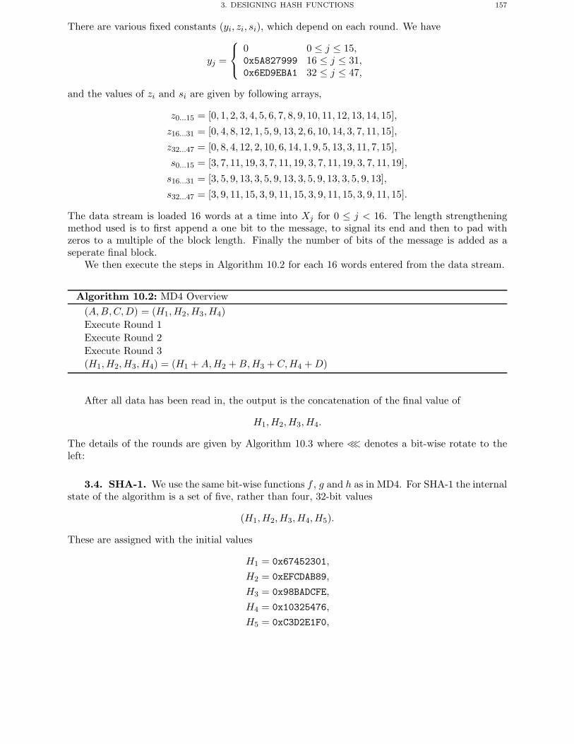
3. DESIGNING HASH FUNCTIONS 157
There are various fixed constants (yi, zi, si), which depend on each round. We have
yj =
⎧⎨⎩
0 0 ≤ j ≤ 15,0x5A827999 16 ≤ j ≤ 31,0x6ED9EBA1 32 ≤ j ≤ 47,
and the values of zi and si are given by following arrays,
z0...15 = [0, 1, 2, 3, 4, 5, 6, 7, 8, 9, 10, 11, 12, 13, 14, 15],
z16...31 = [0, 4, 8, 12, 1, 5, 9, 13, 2, 6, 10, 14, 3, 7, 11, 15],
z32...47 = [0, 8, 4, 12, 2, 10, 6, 14, 1, 9, 5, 13, 3, 11, 7, 15],
s0...15 = [3, 7, 11, 19, 3, 7, 11, 19, 3, 7, 11, 19, 3, 7, 11, 19],
s16...31 = [3, 5, 9, 13, 3, 5, 9, 13, 3, 5, 9, 13, 3, 5, 9, 13],
s32...47 = [3, 9, 11, 15, 3, 9, 11, 15, 3, 9, 11, 15, 3, 9, 11, 15].
The data stream is loaded 16 words at a time into Xj for 0 ≤ j < 16. The length strengtheningmethod used is to first append a one bit to the message, to signal its end and then to pad withzeros to a multiple of the block length. Finally the number of bits of the message is added as aseperate final block.
We then execute the steps in Algorithm 10.2 for each 16 words entered from the data stream.
Algorithm 10.2: MD4 Overview(A,B,C,D) = (H1,H2,H3,H4)Execute Round 1Execute Round 2Execute Round 3(H1,H2,H3,H4) = (H1 +A,H2 +B,H3 + C,H4 +D)
After all data has been read in, the output is the concatenation of the final value of
H1,H2,H3,H4.
The details of the rounds are given by Algorithm 10.3 where ≪ denotes a bit-wise rotate to theleft:
3.4. SHA-1. We use the same bit-wise functions f , g and h as in MD4. For SHA-1 the internalstate of the algorithm is a set of five, rather than four, 32-bit values
(H1,H2,H3,H4,H5).
These are assigned with the initial values
H1 = 0x67452301,H2 = 0xEFCDAB89,H3 = 0x98BADCFE,H4 = 0x10325476,H5 = 0xC3D2E1F0,
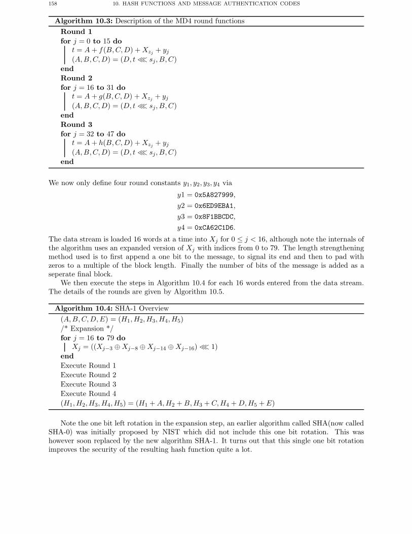
158 10. HASH FUNCTIONS AND MESSAGE AUTHENTICATION CODES
Algorithm 10.3: Description of the MD4 round functionsRound 1for j = 0 to 15 do
t = A+ f(B,C,D) +Xzj + yj(A,B,C,D) = (D, t ≪ sj, B,C)
endRound 2for j = 16 to 31 do
t = A+ g(B,C,D) +Xzj + yj(A,B,C,D) = (D, t ≪ sj, B,C)
endRound 3for j = 32 to 47 do
t = A+ h(B,C,D) +Xzj + yj(A,B,C,D) = (D, t ≪ sj, B,C)
end
We now only define four round constants y1, y2, y3, y4 via
y1 = 0x5A827999,y2 = 0x6ED9EBA1,y3 = 0x8F1BBCDC,y4 = 0xCA62C1D6.
The data stream is loaded 16 words at a time into Xj for 0 ≤ j < 16, although note the internals ofthe algorithm uses an expanded version of Xj with indices from 0 to 79. The length strengtheningmethod used is to first append a one bit to the message, to signal its end and then to pad withzeros to a multiple of the block length. Finally the number of bits of the message is added as aseperate final block.
We then execute the steps in Algorithm 10.4 for each 16 words entered from the data stream.The details of the rounds are given by Algorithm 10.5.
Algorithm 10.4: SHA-1 Overview(A,B,C,D,E) = (H1,H2,H3,H4,H5)/* Expansion */for j = 16 to 79 do
Xj = ((Xj−3 ⊕Xj−8 ⊕Xj−14 ⊕Xj−16) ≪ 1)endExecute Round 1Execute Round 2Execute Round 3Execute Round 4(H1,H2,H3,H4,H5) = (H1 +A,H2 +B,H3 + C,H4 +D,H5 +E)
Note the one bit left rotation in the expansion step, an earlier algorithm called SHA(now calledSHA-0) was initially proposed by NIST which did not include this one bit rotation. This washowever soon replaced by the new algorithm SHA-1. It turns out that this single one bit rotationimproves the security of the resulting hash function quite a lot.
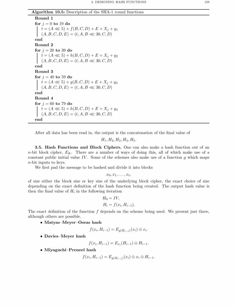
3. DESIGNING HASH FUNCTIONS 159
Algorithm 10.5: Description of the SHA-1 round functionsRound 1for j = 0 to 19 do
t = (A ≪ 5) + f(B,C,D) + E +Xj + y1
(A,B,C,D,E) = (t, A,B ≪ 30, C,D)endRound 2for j = 20 to 39 do
t = (A ≪ 5) + h(B,C,D) + E +Xj + y2
(A,B,C,D,E) = (t, A,B ≪ 30, C,D)endRound 3for j = 40 to 59 do
t = (A ≪ 5) + g(B,C,D) + E +Xj + y3
(A,B,C,D,E) = (t, A,B ≪ 30, C,D)endRound 4for j = 60 to 79 do
t = (A ≪ 5) + h(B,C,D) + E +Xj + y4
(A,B,C,D,E) = (t, A,B ≪ 30, C,D)end
After all data has been read in, the output is the concatenation of the final value of
H1,H2,H3,H4,H5.
3.5. Hash Functions and Block Ciphers. One can also make a hash function out of ann-bit block cipher, EK . There are a number of ways of doing this, all of which make use of aconstant public initial value IV . Some of the schemes also make use of a function g which mapsn-bit inputs to keys.
We first pad the message to be hashed and divide it into blocks
x0, x1, . . . , xt,
of size either the block size or key size of the underlying block cipher, the exact choice of sizedepending on the exact definition of the hash function being created. The output hash value isthen the final value of Hi in the following iteration
H0 = IV,
Hi = f(xi,Hi−1).
The exact definition of the function f depends on the scheme being used. We present just three,although others are possible.
• Matyas–Meyer–Oseas hash
f(xi,Hi−1) = Eg(Hi−1)(xi) ⊕ xi.
• Davies–Meyer hash
f(xi,Hi−1) = Exi(Hi−1) ⊕Hi−1.
• Miyaguchi–Preneel hash
f(xi,Hi−1) = Eg(Hi−1)(xi) ⊕ xi ⊕Hi−1.
160 10. HASH FUNCTIONS AND MESSAGE AUTHENTICATION CODES
4. Message Authentication Codes
Given a message and its hash code, as output by a cryptographic hash function, ensures thatdata has not been tampered with between the execution of the hash function and its verification,by recomputing the hash. However, using a hash function in this way requires the hash code itselfto be protected in some way, by for example a digital signature, as otherwise the hash code itselfcould be tampered with.
To avoid this problem one can use a form of keyed hash function called a message authenticationcode, or MAC. This is a symmetric key algorithm in that the person creating the code and theperson verifying it both require the knowledge of a shared secret.
Suppose two parties, who share a secret key, wish to ensure that data transmitted betweenthem has not been tampered with. They can then use the shared secret key and a keyed algorithmto produce a check-value, or MAC, which is sent with the data. In symbols we compute
code = MACk(m)
where• MAC is the check function,• k is the secret key,• m is the message.
Note we do not assume that the message is secret, we are trying to protect data integrity and notconfidentiality. If we wish our message to remain confidential then we should encrypt it beforeapplying the MAC. After performing the encryption and computing the MAC, the user transmits
ek1(m)‖MACk2 (ek1(m)) .
This is a form of encryption called a data encapsulation mechanism, or DEM for short. Note, thatdifferent keys are used for the encryption and the MAC part of the message and that the MAC isapplied to the ciphertext and not the message.
Before we proceed on how to construct MAC functions it is worth pausing to think about whatsecurity properties we require. We would like that only people who know the shared secret are ableto both produce new MACs or verify existing MACs. In particular it should be hard given a MACon a message to produce a MAC on a new message.
4.1. Producing MACs from hash functions. A collision-free cryptographic hash functioncan also be used as the basis of a MAC. The first idea one comes up with to construct such a MACis to concatenate the key with the message and then apply the hash function. For example
MACk(M ) = h(k‖M ).
However, this is not a good idea since almost all hash functions are created using methods likethe Merkle–Damgard construction. This allows us to attack such a MAC as follows: We assumethat first that the non-length strengthed Merkle–Damgard construction is used with compressionfunction f . Suppose one obtains the MAC c1 on the t block message m1
c1 = MACk(m1) = h(k‖m1)
We can then, without knowledge of k compute the MAC c2 on the t+ 1 block message m1‖m2 forany m2 of one block in length, via
c2 = MACk(m1‖m2)= f(c1‖m2).
Clearly this attack can be extended to a appending an m2 of arbitrary length. Hence, we can alsoapply it to the length strengthed version. If we let m1 denote a t block message and let b denote
4. MESSAGE AUTHENTICATION CODES 161
the block which encodes the bit length of m1 and we let m2 denote an arbitrary new block, thenfrom the MAC of the message m1 one can obtain the MAC of the message
m1‖b‖m2.
Having worked out that prepending a key to a message does not give a secure MAC, one mightbe led to try appending the key after the message as in
MACk(M ) = h(M‖k).Again we now can make use of the Merkle–Damgard construction to produce an attack. We first,without knowledge of k, find via a birthday attack on the hash function h two equal length messagesm1 and m2 which hash to the same values:
h(m1) = h(m2).
We now try to obtain the legitimate MAC c1 on the message m1. From, this we can deduce theMAC on the message m2 via
MACk(m2) = h(m2‖k)= f (h(m2)‖k)= f (h(m1)‖k)= h(m1‖k)= MACk(m1)= c1.
assuming k is a single block in length and the non-length strengthened version is used. Both ofthese assumptions can be relaxed, the details of which we leave to the reader.
To produce a secure MAC from a hash function one needs to be a little more clever. A MAC,called HMAC, occurring in a number of standards documents works as follows:
HMAC = h(k‖p1‖h(k‖p2‖M )),
where p1 and p2 are strings used to pad out the input to the hash function to a full block.
4.2. Producing MACs from block ciphers. Apart from ensuring the confidentiality ofmessages, block ciphers can also be used to protect the integrity of data. There are various typesof MAC schemes based on block ciphers, but the best known and most widely used by far are theCBC-MACs. These are generated by a block cipher in CBC Mode. CBC-MACs are the subject ofvarious international standards dating back to the early 1980s. These early standards specify theuse of DES in CBC mode to produce a MAC, although one could really use any block cipher inplace of DES.
Using an n-bit block cipher to give an m-bit MAC, where m ≤ n, is done as follows:
• The data is padded to form a series of n-bit blocks.• The blocks are encrypted using the block cipher in CBC Mode.• Take the final block as the MAC, after an optional postprocessing stage and truncation
(if m < n).
Hence, if the n-bit data blocks are
m1,m2, . . . ,mq
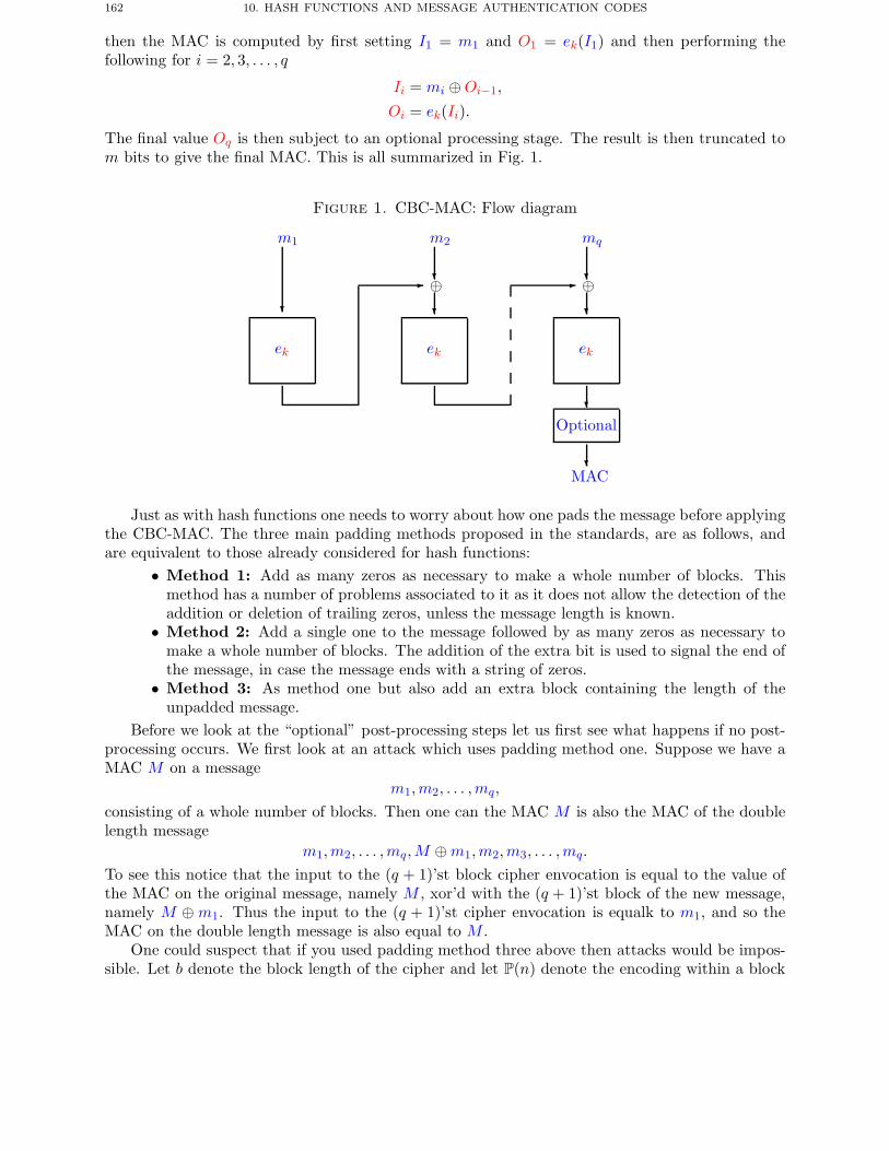
162 10. HASH FUNCTIONS AND MESSAGE AUTHENTICATION CODES
then the MAC is computed by first setting I1 = m1 and O1 = ek(I1) and then performing thefollowing for i = 2, 3, . . . , q
Ii = mi ⊕Oi−1,
Oi = ek(Ii).
The final value Oq is then subject to an optional processing stage. The result is then truncated tom bits to give the final MAC. This is all summarized in Fig. 1.
Figure 1. CBC-MAC: Flow diagram
m1
ek
m2
⊕
ek
mq
⊕
ek
Optional
MAC
Just as with hash functions one needs to worry about how one pads the message before applyingthe CBC-MAC. The three main padding methods proposed in the standards, are as follows, andare equivalent to those already considered for hash functions:
• Method 1: Add as many zeros as necessary to make a whole number of blocks. Thismethod has a number of problems associated to it as it does not allow the detection of theaddition or deletion of trailing zeros, unless the message length is known.
• Method 2: Add a single one to the message followed by as many zeros as necessary tomake a whole number of blocks. The addition of the extra bit is used to signal the end ofthe message, in case the message ends with a string of zeros.
• Method 3: As method one but also add an extra block containing the length of theunpadded message.
Before we look at the “optional” post-processing steps let us first see what happens if no post-processing occurs. We first look at an attack which uses padding method one. Suppose we have aMAC M on a message
m1,m2, . . . ,mq,
consisting of a whole number of blocks. Then one can the MAC M is also the MAC of the doublelength message
m1,m2, . . . ,mq,M ⊕m1,m2,m3, . . . ,mq.
To see this notice that the input to the (q + 1)’st block cipher envocation is equal to the value ofthe MAC on the original message, namely M , xor’d with the (q + 1)’st block of the new message,namely M ⊕m1. Thus the input to the (q + 1)’st cipher envocation is equalk to m1, and so theMAC on the double length message is also equal to M .
One could suspect that if you used padding method three above then attacks would be impos-sible. Let b denote the block length of the cipher and let P(n) denote the encoding within a block
Chapter Summary 163
of the number n. To MAC a single block message m1 one then computes
M1 = ek (ek(m1) ⊕ P(b)) .
Suppose one obtains the MAC’s M1 and M2 on the single block messages m1 and m2. Then onerequests the MAC on the three block message
m1,P(b),m3
for some new block m3. Suppose the recieved MAC is then equal to M3, i.e.
M3 = ek (ek (ek (ek(m1) ⊕ P(b)) ⊕m3) ⊕ P(3b)) .
Now also consider the MAC on the three block message
m2,P(b),m3 ⊕M1 ⊕M2.
This MAC is equal to M ′3, where
M ′3 = ek (ek (ek (ek(m2) ⊕ P(b)) ⊕m3 ⊕M1 ⊕M2) ⊕ P(3b))
= ek (ek (ek (ek(m2) ⊕ P(b)) ⊕m3 ⊕ ek (ek(m1) ⊕ P(b)) ⊕ ek (ek(m2) ⊕ P(b)))⊕P(3b))
= ek (ek (m3 ⊕ ek (ek(m1) ⊕ P(b))) ⊕ P(3b))= ek (ek (ek (ek(m1) ⊕ P(b)) ⊕m3) ⊕ P(3b))= M3.
Hence, we see that on their own the non-trivial padding methods do not protect against MACforgery attacks. This is one of the reasons for introducing the post processing steps. There are twopopular post-processing steps, designed to make it more difficult for the cryptanalyst to performan exhaustive key search and to protect against attacks such as the ones explained above:
(1) Choose a key k1 and compute
Oq = ek (dk1(Oq)) .
(2) Choose a key k1 and compute
Oq = ek1(Oq).
Both of these post-processing steps were invented when DES was the dominant cipher, and in sucha situation the first of these is equivalent to processing the final block of the message using the3DES algorithm.
Chapter Summary
• Hash functions are required which are both preimage, collision and second-preimage resis-tant.
• Due to the birthday paradox the output of the hash function should be at least twice thesize of what one believes to be the limit of the computational ability of the attacker.
• More hash functions are iterative in nature, although most of the currently deployed oneshave recently shown to be weaker than expected.
• A message authentication code is in some sense a keyed hash function.• MACs can be created out of either block ciphers or hash functions.
164 10. HASH FUNCTIONS AND MESSAGE AUTHENTICATION CODES
Further Reading
A detailed description of both SHA-1 and the SHA-2 algorithms can be found in the FIPSstandard below, this includes a set of test vectors as well. The recent work on the analysis ofSHA-1, and references to the earlier attacks on MD4 and MD5 can be found in the papers og Wanget. al., of which we list only one below.
FIPS PUB 180-2, Secure Hash Standard (including SHA-1, SHA-256, SHA-384, and SHA-512).NIST, 2005.
X. Wang, Y.L. Yin and H. Yu. Finding Collisions in the Full SHA-1 In Advances in Cryptology –CRYPTO 2005, Springer-Verlag LNCS 3621, pp 17-36, 2005.
Part 3
Public Key Encryption and Signatures
Public key techniques were originally invented to solve the key distribution problem and toprovide authenticity. They have many advantages over symmetric systems, the main one is thatthey do not require two communicating parties to know each other before encrypted communicationcan take place. In addition the use of digital signatures allows users to sign digital data such aselectronic orders or money transfers. Hence, public key technology is one of the key enablingtechnologies for e-commerce and a digital society.

CHAPTER 11
Basic Public Key Encryption Algorithms
Chapter Goals
• To learn about public key encryption and the hard problems on which it is based.• To understand the RSA algorithm and the assumptions on which its security relies.• To understand the ElGamal encryption algorithm and it assumptions.• To learn about the Rabin encryption algorithm and its assumptions.• To learn about the Paillier encryption algorithm and its assumptions.
1. Public Key Cryptography
Recall that in symmetric key cryptography each communicating party needed to have a copyof the same secret key. This led to a very difficult key management problem. In public keycryptography we replace the use of identical keys with two keys, one public and one private.
The public key can be published in a directory along with the user’s name. Anyone who thenwishes to send a message to the holder of the associated private key will take the public key, encrypta message under it and send it to the owner of the corresponding private key. The idea is thatonly the holder of the private key will be able to decrypt the message. More clearly, we have thetransforms
Message + Alice’s public key = Ciphertext,Ciphertext + Alice’s private key = Message.
Hence anyone with Alice’s public key can send Alice a secret message. But only Alice can decryptthe message, since only Alice has the corresponding private key.
Public key systems work because the two keys are linked in a mathematical way, such thatknowing the public key tells you nothing about the private key. But knowing the private key allowsyou to unlock information encrypted with the public key. This may seem strange, and will requiresome thought and patience to understand. The concept was so strange it was not until 1976 thatanyone thought of it. The idea was first presented in the seminal paper of Diffie and Hellmanentitled New Directions in Cryptography. Although Diffie and Hellman invented the concept ofpublic key cryptography it was not until a year or so later that the first (and most successful)system, namely RSA, was invented.
The previous paragraph is how the ‘official’ history of public key cryptography goes. However,in the late 1990s an unofficial history came to light. It turned out that in 1969, over five yearsbefore Diffie and Hellman invented public key cryptography, a cryptographer called James Ellis,working for the British government’s communication headquarters GCHQ, invented the concept ofpublic key cryptography (or non-secret encryption as he called it) as a means of solving the keydistribution problem. Ellis, just like Diffie and Hellman, did not however have a system.
The problem of finding such a public key encryption system was given to a new recruit toGCHQ called Clifford Cocks in 1973. Within a day Cocks had invented what was essentially theRSA algorithm, although a full four years before Rivest, Shamir and Adleman. In 1974 another
167
168 11. BASIC PUBLIC KEY ENCRYPTION ALGORITHMS
employee at GCHQ, Malcolm Williamson, invented the concept of Diffie–Hellman key exchange,which we shall return to in Chapter 14. Hence, by 1974 the British security services had alreadydiscovered the main techniques in public key cryptography.
There is a surprisingly small number of ideas behind public key encryption algorithms, whichmay explain why once Diffie and Hellman or Ellis had the concept of public key encryption, aninvention of essentially the same cipher, i.e. RSA, came so quickly. There are so few ideas becausewe require a mathematical operation which is easy to do one way, i.e. encryption, but which is hardto do the other way, i.e. decryption, without some special secret information, namely the privatekey. Such a mathematical function is called a trapdoor one-way function, since it is effectively aone-way function unless one knows the key to the trapdoor.
Luckily there are a number of possible one-way functions which have been well studied, suchas factoring integers, computing discrete logarithms or computing square roots modulo a compos-ite number. In the next section we shall study such one-way functions, before presenting somepublic key encryption algorithms later in the chapter. However, these are only computational one-way functions in that given enough computing power one can invert these functions faster thanexhaustive search.
2. Candidate One-way Functions
The most important one-way function used in public key cryptography is that of factoringintegers. By factoring an integer we mean finding its prime factors, for example
10 = 2 · 560 = 22 · 3 · 5
2113 − 1 = 3391 · 23 279 · 65 993 · 1 868 569 · 1 066 818 132 868 207
Finding the factors is an expensive computational operation. To measure the complexity of algo-rithms to factor an integer N we often use the function
LN (α, β) = exp((β + o(1))(logN)α(log logN)1−α
).
Notice that if an algorithm to factor an integer has complexity O(LN (0, β)), then it runs in poly-nomial time (recall the input size of the problem is logN). However, if an algorithm to factor aninteger has complexity O(LN (1, β)) then it runs in exponential time. Hence, the function LN (α, β)for 0 < α < 1 interpolates between polynomial and exponential time. An algorithm with complexityO(LN (α, β)) for 0 < α < 1 is said to have sub-exponential behaviour. Notice that multiplication,which is the inverse algorithm to factoring, is a very simple operation requiring time less thanO(LN (0, 2)).
There are a number of methods to factor numbers of the form
N = p · q,some of which we shall discuss in a later chapter. For now we just summarize the most well-knowntechniques.
• Trial Division: Try every prime number up to√N and see if it is a factor of N . This
has complexity LN (1, 1), and is therefore an exponential algorithm.• Elliptic Curve Method: This is a very good method if p < 250, its complexity isLp(1/2, c), which is sub-exponential. Notice that the complexity is given in terms of thesize of the unknown value p. If the number is a product of two primes of very unequal sizethen the elliptic curve method may be the best at finding the factors.
• Quadratic Sieve: This is probably the fastest method for factoring integers of between80 and 100 decimal digits. It has complexity LN (1/2, 1).
2. CANDIDATE ONE-WAY FUNCTIONS 169
• Number Field Sieve: This is currently the most successful method for numbers withmore than 100 decimal digits. It can factor numbers of the size of 10155 ≈ 2512 and hascomplexity LN (1/3, 1.923).
There are a number of other hard problems related to factoring which can be used to producepublic key cryptosystems. Suppose you are given N but not its factors p and q, there are four mainproblems which one can try to solve:
• FACTORING: Find p and q.• RSA: Given e such that
gcd (e, (p − 1)(q − 1)) = 1
and c, find m such thatme = c (mod N).
• QUADRES: Given a, determine whether a is a square modulo N .• SQRROOT: Given a such that
a = x2 (mod N),
find x.Another important class of problems are those based on the discrete logarithm problem or itsvariants. Let (G, ·) be a finite abelian group, such as the multiplicative group of a finite field orthe set of points on an elliptic curve over a finite field. The discrete logarithm problem, or DLP, inG is given g, h ∈ G, find an integer x (if it exists) such that
gx = h.
For some groups G this problem is easy. For example if we take G to be the integers modulo anumber N under addition then given g, h ∈ Z/NZ we need to solve
x · g = h.
We have already seen in Chapter 1 that we can easily tell whether such an equation has a solution,and determine its solution when it does, using the extended Euclidean algorithm.
For certain other groups determining discrete logarithms is believed to be hard. For examplein the multiplicative group of a finite field the best known algorithm for this task is the NumberField Sieve. The complexity of determining discrete logarithms in this case is given by
LN (1/3, c)
for some constant c, depending on the type of the finite field, e.g. whether it is a large prime fieldor an extension field of characteristic two.
For other groups, such as elliptic curve groups, the discrete logarithm problem is believed to beeven harder. The best known algorithm for finding discrete logarithms on a general elliptic curvedefined over a finite field Fq is Pollard’s Rho method which has complexity
√q = Lq(1, 1/2).
Hence, this is a fully exponential algorithm. Since determining elliptic curve discrete logarithms isharder than in the case of multiplicative groups of finite fields we are able to use smaller groups.This leads to an advantage in key size. Elliptic curve cryptosystems often have much smaller keysizes (say 160 bits) compared with those based on factoring or discrete logarithms in finite fields(where for both the ‘equivalent’ recommended key size is about 1024 bits).
Just as with the FACTORING problem, there are a number of related problems associated todiscrete logarithms; again suppose we are given a finite abelian group (G, ·) and g ∈ G.
• DLP: This is the discrete logarithm problem considered above. Namely given g, h ∈ Gsuch that h = gx, find x.
170 11. BASIC PUBLIC KEY ENCRYPTION ALGORITHMS
• DHP: This is the Diffie–Hellman problem. Given g ∈ G and
a = gx and b = gy,
find c such thatc = gxy.
• DDH: This is the decision Diffie–Hellman problem. Given g ∈ G and
a = gx, b = gy and c = gz,
determine if z = x · y.
When giving all these problems it is important to know how they are all related. This is doneby giving complexity theoretic reductions from one problem to another. This allows us to say that‘Problem A is no harder than Problem B’. We do this by assuming an oracle (or efficient algorithm)to solve Problem B. We then use this oracle to give an efficient algorithm for Problem A. Hence, wereduce the problem of solving Problem A to inventing an efficient algorithm to solve Problem B.The algorithms which perform these reductions should be efficient, in that they run in polynomialtime, where we treat each oracle query as a single step.
We can also show equivalence between two problems A and B, by showing an efficient reductionfrom A to B and an efficient reduction from B to A. If the two reductions are both polynomial-timereductions then we say that the two problems are polynomial-time equivalent.
As an example we first show how to reduce solving the Diffie–Hellman problem to the discretelogarithm problem.
Lemma 11.1. In an arbitrary finite abelian group G the DHP is no harder than the DLP.
Proof. Suppose I have an oracle ODLP which will solve the DLP for me, i.e. on input of h = gx
it will return x. To solve the DHP on input of a = gx and b = gy we compute(1) z = ODLP(a).(2) c = bz.(3) Output c.
The above reduction clearly runs in polynomial time and will compute the true solution to theDHP, assuming the oracle returns the correct value, i.e.
z = x.
Hence, the DHP is no harder than the DLP. �
In some groups there is a more complicated argument to show that the DHP is in fact equivalentto the DLP.
We now show how to reduce the solution of the decision Diffie–Hellman problem to the Diffie–Hellman problem, and hence using our previous argument to the discrete logarithm problem.
Lemma 11.2. In an arbitrary finite abelian group G the DDH is no harder than the DHP.
Proof. Now suppose we have an oracle ODHP which on input of gx and gy computes the valueof gxy. To solve the DDH on input of a = gx, b = gy and c = gz we compute
(1) d = ODHP(a, b).(2) If d = c output YES.(3) Else output NO.
Again the reduction clearly runs in polynomial time, and assuming the output of the oracle iscorrect then the above reduction will solve the DDH. �
2. CANDIDATE ONE-WAY FUNCTIONS 171
So the decision Diffie–Hellman problem is no harder than the computational Diffie–Hellmanproblem. There are however some groups in which one can solve the DDH in polynomial time butthe fastest known algorithm to solve the DHP takes sub-exponential time.
Hence, of our three discrete logarithm based problems, the easiest is DDH, then comes DHPand finally the hardest problem is DLP.
We now turn to show reductions for the factoring based problems. The most important resultis
Lemma 11.3. The FACTORING and SQRROOT problems are polynomial-time equivalent.
Proof. We first show how to reduce SQRROOT to FACTORING. Assume we are given afactoring oracle, we wish to show how to use this to extract square roots modulo a compositenumber N . Namely, given
z = x2 (mod N)we wish to compute x. First we factor N into its prime factors pi using the factoring oracle. Thenwe compute
si =√z (mod pi),
this can be done in expected polynomial time using Shanks’ Algorithm. Then we compute thevalue of x using the Chinese Remainder Theorem on the data
si =√z (mod pi).
One has to be a little careful if powers of pi greater than one divide N , but this is easy to deal withand will not concern us here. Hence, finding square roots modulo N is no harder than factoring.
We now show that FACTORING can be reduced to SQRROOT. Assume we are given an oraclefor extracting square roots modulo a composite number N . We shall assume for simplicity that Nis a product of two primes, which is the most difficult case. The general case is only slightly moretricky mathematically, but it is computationally easier since factoring numbers with three or moreprime factors is usually easier than factoring numbers with two prime factors.
We wish to use our oracle for the problem SQRROOT to factor the integer N into its primefactors, i.e. given N = p · q we wish to compute p. First we pick a random x ∈ (Z/NZ)∗ andcompute
z = x2 (mod N).Now we compute
y =√z (mod N)
using the SQRROOT oracle. There are four such square roots, since N is a product of two primes.With 50 percent probability we obtain
y �= ±x (mod N).
If we do not obtain this inequality then we simply repeat the method. We expect after an averagenumber of two repetitions we will obtain the desired inequality.
Now, since x2 = y2 (mod N), we see that N divides
x2 − y2 = (x− y)(x+ y).
But N does not divide either x− y or x+ y, since y �= ±x (mod N). So the factors of N must bedistributed over these later two pairs of numbers. This means we can obtain a non-trivial factor ofN by computing gcd(x− y,N)
Clearly both of the above reductions can be performed in expected polynomial time. Hence,the problems FACTORING and SQRROOT are polynomial-time equivalent. �
172 11. BASIC PUBLIC KEY ENCRYPTION ALGORITHMS
The above proof contains an important tool used in factoring algorithms, namely the construc-tion of a difference of two squares. We shall return to this later in Chapter 12.
Before leaving the problem SQRROOT notice that QUADRES is easier than SQRROOT, sincean algorithm to compute square roots modulo N can be used to determine quadratic residuosity.
Finally we end this section by showing that the RSA problem can be reduced to FACTORING.Recall the RSA problem is given c = me (mod N), find m.
Lemma 11.4. The RSA problem is no harder than the FACTORING problem.
Proof. Using a factoring oracle we first find the factorization of N . We can now computeΦ = φ(N) and then compute
d = 1/e (mod Φ).
Once d has been computed it is easy to recover m via
cd = med = m1 (mod Φ) = m (mod N).
Hence, the RSA problem is no harder than FACTORING. �
There is some evidence, although slight, that the RSA problem may actually be easier thanFACTORING for some problem instances. It is a major open question as to how much easier it is.
3. RSA
The RSA algorithm was the world’s first public key encryption algorithm, and it has stood thetest of time remarkably well. The RSA algorithm is based on the difficulty of the RSA problemconsidered in the previous section, and hence it is based on the difficulty of finding the prime factorsof large integers. We have seen that it may be possible to solve the RSA problem without factoring,hence the RSA algorithm is not based completely on the difficulty of factoring.
Suppose Alice wishes to enable anyone to send her secret messages, which only she can decrypt.She first picks two large secret prime numbers p and q. Alice then computes
N = p · q.Alice also chooses an encryption exponent e which satisfies
gcd(e, (p − 1)(q − 1)) = 1.
It is common to choose e = 3, 17 or 65 537. Now Alice’s public key is the pair (N, e), which shecan publish in a public directory. To compute the private key Alice applies the extended Euclideanalgorithm to e and (p− 1)(q − 1) to obtain the decryption exponent d, which should satisfy
e · d ≡ 1 (mod (p− 1)(q − 1)).
Alice keeps secret her private key, which is the triple (d, p, q). Actually, she could simply throwaway p and q, and retain a copy of her public key which contains the integer N , but we shall seelater that this is not efficient.
Now suppose Bob wishes to encrypt a message to Alice. He first looks up Alice’s public keyand represents the message as a number m which is strictly less than the public modulus N . Theciphertext is then produced by raising the message to the power of the public encryption exponentmodulo the public modulus, i.e.
c = me (mod N).
Alice on receiving c can decrypt the ciphertext to recover the message by exponentiating by theprivate decryption exponent, i.e.
m = cd (mod N).
3. RSA 173
This works since the group (Z/NZ)∗ has order
φ(N ) = (p − 1)(q − 1)
and so, by Lagrange’s Theorem,
x(p−1)(q−1) ≡ 1 (mod N),
for all x ∈ (Z/NZ)∗. For some integer s we have
ed− s(p− 1)(q − 1) = 1,
and so
cd = (me)d
= med
= m1+s(p−1)(q−1)
= m ·ms(p−1)(q−1)
= m.
To make things clearer let’s consider a baby example. Choose p = 7 and q = 11, and so N = 77and (p− 1)(q − 1) = 6 · 10 = 60. We pick as the public encryption exponent e = 37, since we havegcd(37, 60) = 1. Then, applying the extended Euclidean algorithm we obtain d = 13 since
37 · 13 = 481 = 1 (mod 60).
Suppose the message we wish to transmit is given by m = 2, then to encrypt m we compute
c = me (mod N) = 237 (mod 77) = 51,
whilst to decrypt the ciphertext c we compute
m = cd (mod N) = 5113 (mod 77) = 2.
3.1. RSA Encryption and the RSA Problem. The security of RSA on first inspectionrelies on the difficulty of finding the private encryption exponent d given only the public key, namelythe public modulus N and the public encryption exponent e.
We have shown that the RSA problem is no harder than FACTORING, hence if we can factor Nthen we can find p and q and hence we can calculate d. Hence, if factoring is easy we can break RSA.Currently 500-bit numbers are the largest that have been factored and so it is recommended thatone takes public moduli of size around 1024 bits to ensure medium-term security. For long-termsecurity one would need to take a public modulus size of over 2048 bits.
In this chapter we shall consider security to be defined as being unable to recover the wholeplaintext given the ciphertext. We shall argue in a later chapter that this is far too weak a definitionof security for many applications. In addition in a later chapter we shall show that RSA, as wehave described it, is not secure against a chosen ciphertext attack.
For a public key algorithm the adversary always has access to the encryption algorithm, henceshe can always mount a chosen plaintext attack. RSA is secure against a chosen plaintext attackassuming our weak definition of security and that the RSA problem is hard. To show this we usethe reduction arguments of the previous section. This example is rather trivial but we labour thepoint since these arguments are used over and over again in later chapters.
Lemma 11.5. If the RSA problem is hard then the RSA system is secure under a chosen plaintextattack, in the sense that an attacker is unable to recover the whole plaintext given the ciphertext.
174 11. BASIC PUBLIC KEY ENCRYPTION ALGORITHMS
Proof. We wish to give an algorithm which solves the RSA problem using an algorithm tobreak the RSA cryptosystem as an oracle. If we can show this then we can conclude that thebreaking the RSA cryptosystem is no harder than solving the RSA problem.
Recall that the RSA problem is given N = p ·q, e and y ∈ (Z/NZ)∗, compute an x such that xe
(mod N) = y. We use our oracle to break the RSA encryption algorithm to ‘decrypt’ the messagecorresponding to c = y, this oracle will return the plaintext message m. Then our RSA problem issolved by setting x = m since, by definition,
me (mod N) = c = y.
So if we can break the RSA algorithm then we can solve the RSA problem. �
3.2. Knowledge of the Private Exponent and Factoring. Whilst it is unclear whetherbreaking RSA, in the sense of inverting the RSA function, is equivalent to factoring, determiningthe private key d given the public information N and e is equivalent to factoring.
Lemma 11.6. If one knows the RSA decryption exponent d corresponding to the public key(N, e) then one can efficiently factor N .
Proof. Recall that for some integer s
ed− 1 = s(p − 1)(q − 1).
We pick an integer x �= 0, this is guaranteed to satisfy
xed−1 = 1 (mod N).
We now compute a square root y1 of one modulo N ,
y1 =√xed−1 = x(ed−1)/2,
which we can do since ed− 1 is known and will be even. We will then have the identity
y12 − 1 ≡ 0 (mod N),
which we can use to recover a factor of N via computing
gcd(y1 − 1,N ).
But this will only work when y1 �= ±1 (mod N).Now suppose we are unlucky and we obtain y1 = ±1 (mod N) rather than a factor of N . If
y1 = −1 (mod N) we return to the beginning and pick another value of x. This leaves us with thecase y1 = 1 (mod N), in which case we take another square root of one via,
y2 =√y1 = x(ed−1)/4.
Again we havey2
2 − 1 = y1 − 1 = 0 (mod N).
Hence we computegcd(y2 − 1,N )
and see if this gives a factor of N . Again this will give a factor of N unless y2 = ±1, if we areunlucky we repeat once more and so on.
This method can be repeated until either we have factored N or until (ed − 1)/2t is no longerdivisible by 2. In this latter case we return to the beginning, choose a new random value of x andstart again. �
3. RSA 175
The algorithm in the above proof is an example of a Las Vegas Algorithm: It is probabilisticin nature in the sense that whilst it may not actually give an answer (or terminate), it is howeverguaranteed that when it does give an answer then that answer will always be correct.
We shall now present a small example of the previous method. Consider the following RSAparameters
N = 1441 499, e = 17 and d = 507 905.Recall we are assuming that the private exponent d is public knowledge. We will show that theprevious method does in fact find a factor of N . Put
t1 = (ed − 1)/2 = 4317 192,x = 2.
To compute y1 we evaluate
y1 = x(ed−1)/2,
= 2t1 ,
= 1 (mod N).
Since we obtain y1 = 1 we need to set
t2 = t1/2 = (ed − 1)/4 = 2158 596,
y2 = 2t2 .
We now compute y2,
y2 = x(ed−1)/4,
= 2t2 ,
= 1 (mod N).
So we need to repeat the method again, this time we obtain t3 = (ed − 1)/8 = 1079 298. Wecompute y3,
y3 = x(ed−1)/8,
= 2t3 ,
= 119 533 (mod N).
Soy3
2 − 1 = (y3 − 1)(y3 + 1) ≡ 0 (mod N),and we compute a prime factor of N by evaluating
gcd(y3 − 1,N ) = 1423.
3.3. Knowledge of φ(N) and Factoring. We have seen that knowledge of d allows us tofactor N . Now we will show that knowledge of Φ = φ(N) also allows us to factor N .
Lemma 11.7. Given an RSA modulus N and the value of Φ = φ(N) one can efficiently factorN .
Proof. We haveΦ = (p− 1)(q − 1) = N − (p+ q) + 1.
Hence, if we set S = N + 1 − Φ, we obtain
S = p+ q.
So we need to determine p and q from their sum S and product N . Define the polynomial
f(X) = (X − p) · (X − q) = X2 − SX +N.
176 11. BASIC PUBLIC KEY ENCRYPTION ALGORITHMS
So we can find p and q by solving f(X) = 0 using the standard formulae for extracting the rootsof a quadratic polynomial,
p =S +
√S2 − 4N2
,
q =S −√
S2 − 4N2
.
�
As an example consider the RSA public modulus N = 18923. Assume that we are givenΦ = φ(N) = 18 648. We then compute
S = p+ q = N + 1 − Φ = 276.
Using this we compute the polynomial
f(X) = X2 − SX +N = X2 − 276X + 18923
and find that its roots over the real numbers are
p = 149, q = 127
which are indeed the factors of N .
3.4. Use of a Shared Modulus. Since modular arithmetic is very expensive it can be verytempting for a system to be set up in which a number of users share the same public modulus Nbut use different public/private exponents, (ei, di). One reason to do this could be to allow veryfast hardware acceleration of modular arithmetic, specially tuned to the chosen shared modulus N .This is, however, a very silly idea since it can be attacked in one of two ways, either by a maliciousinsider or by an external attacker.
Suppose the bad guy is one of the internal users, say user number one. He can now computethe value of the decryption exponent for user number two, namely d2. First user one computes pand q since they know d1, via the algorithm in the proof of Lemma 11.6. Then user one computesφ(N) = (p− 1)(q − 1), and finally they can recover d2 from
d2 =1e2
(mod φ(N)).
Now suppose the attacker is not one of the people who share the modulus. Suppose Alice sendsthe same message m to two of the users with public keys
(N, e1) and (N, e2),
i.e. N1 = N2 = N . Eve, the external attacker, sees the messages c1 and c2 where
c1 = me1 (mod N),
c2 = me2 (mod N).
Eve can now compute
t1 = e1−1 (mod e2),
t2 = (t1e1 − 1)/e2,
3. RSA 177
and can recover the message m from
ct11 c−t22 = me1t1m−e2t2
= m1+e2t2m−e2t2
= m1+e2t2−e2t2
= m1 = m.
As an example of this external attack, take the public keys as
N = N1 = N2 = 18923, e1 = 11 and e2 = 5.
Now suppose Eve sees the ciphertexts
c1 = 1514 and c2 = 8189
corresponding to the same plaintext m. Then Eve computes t1 = 1 and t2 = 2, and recovers themessage
m = ct11 c−t22 = 100 (mod N).
3.5. Use of a Small Public Exponent. Fielded RSA systems often use a small publicexponent e so as to cut down the computational cost of the sender. We shall now show that thiscan also lead to problems. Suppose we have three users all with different public moduli
N1, N2 and N3.
In addition suppose they all have the same small public exponent e = 3. Suppose someone sendsthem the same message m.
The attacker Eve sees the messages
c1 = m3 (mod N1),
c2 = m3 (mod N2),
c3 = m3 (mod N3).
Now the attacker, using the Chinese Remainder Theorem, computes the simultaneous solution to
X = ci (mod Ni) for i = 1, 2, 3,
to obtainX = m3 (mod N1N2N3).
But since m3 < N1N2N3 we must have X = m3 identically over the integers. Hence we can recoverm by taking the real cube root of X .
As a simple example of this attack take,
N1 = 323, N2 = 299 and N3 = 341.
Suppose Eve sees the ciphertexts
c1 = 50, c2 = 268 and c3 = 1,
and wants to determine the common value ofm. Eve computes via the Chinese Remainder Theorem
X = 300 763 (mod N1N2N3).
Finally, she computes over the integers
m = X1/3 = 67.
This attack and the previous one are interesting since we find the message without factoringthe modulus. This is, albeit slight, evidence that breaking RSA is easier than factoring. Themain lesson, however, from both these attacks is that plaintext should be randomly padded beforetransmission. That way the same ‘message’ is never encrypted to two different people. In addition
178 11. BASIC PUBLIC KEY ENCRYPTION ALGORITHMS
one should probably avoid very small exponents for encryption, e = 65537 is the usual choice nowin use. However, small public exponents for RSA signatures (see later) do not seem to have anyproblems.
4. ElGamal Encryption
The simplest encryption algorithm based on the discrete logarithm problem is the ElGamalencryption algorithm. In the following we shall describe the finite field analogue of ElGamalencryption, we leave it as an exercise to write down the elliptic curve variant.
Unlike the RSA algorithm, in ElGamal encryption there are some public parameters which canbe shared by a number of users. These are called the domain parameters and are given by
• p a ‘large prime’, by which we mean one with around 1024 bits, such that p−1 is divisibleby another ‘medium prime’ q of around 160 bits.
• g an element of F∗p of prime order q, i.e.
g = r(p−1)/q (mod p) �= 1 for some r ∈ F∗p.
All the domain parameters do is create a public finite abelian group G of prime order q withgenerator g. Such domain parameters can be shared between a large number of users.
Once these domain parameters have been fixed, the public and private keys can then be deter-mined. The private key is chosen to be an integer x, whilst the public key is given by
h = gx (mod p).
Notice that whilst each user in RSA needed to generate two large primes to set up their key pair(which is a costly task), for ElGamal encryption each user only needs to generate a random numberand perform a modular exponentiation to generate a key pair.
Messages are assumed to be non-zero elements of the field F∗p. To encrypt a message m ∈ F∗
p
we• generate a random ephemeral key k,• set c1 = gk,• set c2 = m · hk,• output the ciphertext as c = (c1, c2).
Notice that since each message has a different ephemeral key, encrypting the same message twicewill produce different ciphertexts.
To decrypt a ciphertext c = (c1, c2) we compute
c2c1x
=m · hkgxk
=m · gxkgxk
= m.
As an example of ElGamal encryption consider the following. We first need to set up the domainparameters. For our small example we choose
q = 101, p = 809 and g = 3.
Note that q divides p− 1 and that g has order divisible by q in the multiplicative group of integersmodulo p. The actual order of g is 808 since
3808 = 1 (mod p),
and no smaller power of g is equal to one. As a public private key pair we choose• x = 68,• h = gx = 65.
4. ELGAMAL ENCRYPTION 179
Now suppose we wish to encrypt the message m = 100 to the user with the above ElGamal publickey.
• We generate a random ephemeral key k = 89.• Set c1 = gk = 345.• Set c2 = m · hk = 517.• Output the ciphertext as c = (345, 517).
The recipient can decrypt our ciphertext by computingc2c1x
=517
34568
= 100.
This last value is computed by first computing 34568, taking the inverse modulo p of the result andthen multiplying this value by 517.
In a later chapter we shall see that ElGamal encryption as it stands is not secure against achosen ciphertext attack, so usually a modified scheme is used. However, ElGamal encryption issecure against a chosen plaintext attack, assuming the Diffie–Hellman problem is hard. Again, herewe take a naive definition of what security means in that an encryption algorithm is secure if anadversary is unable to invert the encryption function.
Lemma 11.8. Assuming the Diffie–Hellman problem (DHP) is hard then ElGamal is secure un-der a chosen plaintext attack, where security means it is hard for the adversary, given the ciphertext,to recover the whole of the plaintext.
Proof. To see that ElGamal encryption is secure under a chosen plaintext attack assumingthe Diffie–Hellman problem is hard, we first suppose that we have an oracle O to break ElGamalencryption. This oracle O(h, (c1, c2)) takes as input a public key h and a ciphertext (c1, c2) andthen returns the underlying plaintext. We will then show how to use this oracle to solve the DHP.
Suppose we are givengx and gy
and we are asked to solve the DHP, i.e. we need to compute gxy.We first set up an ElGamal public key which depends on the input to this Diffie–Hellman
problem, i.e. we seth = gx.
Note, we do not know what the corresponding private key is. Now we write down the ‘ciphertext’
c = (c1, c2),
where• c1 = gy,• c2 is a random element of F∗
p.Now we input this ciphertext into our oracle which breaks ElGamal encryption so as to produce thecorresponding plaintext, m = O(h, (c1, c2)). We can now solve the original Diffie–Hellman problemby computing
c2m
=m · hym
since c1 = gy
= hy
= gxy.
�
180 11. BASIC PUBLIC KEY ENCRYPTION ALGORITHMS
5. Rabin Encryption
There is another system, due to Rabin, based on the difficulty of factoring large integers. Infact it is actually based on the difficulty of extracting square roots modulo N = p · q. Recall thatthese two problems are known to be equivalent, i.e.
• knowing the factors of N means we can extract square roots modulo N ,• extracting square roots modulo N means we can factor N .
Hence, in some respects such a system should be considered more secure than RSA. Encryption inthe Rabin encryption system is also much faster than almost any other public key scheme. Despitethese plus points the Rabin system is not used as much as the RSA system. It is, however, usefulto study for a number of reasons, both historical and theoretical. The basic idea of the system isalso used in some higher level protocols.
We first choose prime numbers of the form
p ≡ q ≡ 3 (mod 4)
since this makes extracting square roots modulo p and q very fast. The private key is then the pair(p, q). To compute the associated public key we generate a random integer B ∈ {0, . . . ,N − 1} andthen the public key is
(N,B),
where N is the product of p and q.To encrypt a message m, using the above public key, in the Rabin encryption algorithm we
computec = m(m+B) (mod N).
Hence, encryption involves one addition and one multiplication modulo N . Encryption is thereforemuch faster than RSA encryption, even when one chooses a small RSA encryption exponent.
Decryption is far more complicated, essentially we want to compute
m =
√B2
4+ c− B
2(mod N).
At first sight this uses no private information, but a moment’s thought reveals that you need thefactorization of N to be able to find the square root. There are however four possible square rootsmodulo N , since N is the product of two primes. Hence, on decryption you obtain four possibleplaintexts. This means that we need to add redundancy to the plaintext before encryption in orderto decide which of the four possible plaintexts corresponds to the intended one.
We still need to show why Rabin decryption works. Recall
c = m(m+B) (mod N),
then √B2
4+ c− B
2=
√B2 + 4m(m+B)
4− B
2
=
√4m2 + 4Bm+B2
4− B
2
=
√(2m+B)2
4− B
2
=2m+B
2− B
2= m,
of course assuming the ‘correct’ square root is taken.
6. PAILLIER ENCRYPTION 181
We end with an example of Rabin encryption at work. Let the public and private keys be givenby
• p = 127 and q = 131,• N = 16637 and B = 12345.
To encrypt m = 4410 we compute
c = m(m+B) (mod N) = 4633.
To decrypt we first compute
t = B2/4 + c (mod N) = 1500.
We then evaluate the square root of t modulo p and q√t (mod p) = ±22,
√t (mod q) = ±37.
Now we apply the Chinese Remainder Theorem to both
±22 (mod p) and ±37 (mod q)
so as to find the square root of t modulo N ,
s =√t (mod N) = ±3705 or ±14 373.
The four possible messages are then given by the four possible values of
s− B
2= s− 12 345
2.
This leaves us with the four messages
4410, 5851, 15 078, or 16 519.
6. Paillier Encryption
There is another system, due to Paillier, based on the difficulty of factoring large integers.Paillier’s scheme has a number of interesting properties, such as the fact that it is additivelyhomomorphic (which means it has found application in electronic voting applications).
We first pick an RSA modulo N = p · q, but instead of working with the multiplicative group(Z/NZ)∗ we work with (Z/N2Z)∗. The order of this last group is given by φ(N ) = N ·(p−1)·(q−1) =N · φ(N). Which means, by Lagrange’s Theorem, that for all a with gcd(a,N) = 1 we have
aN ·(p−1)·(q−1) ≡ 1 (mod N2).
The private key for Paillier’s scheme is defined to be an integer d such that
d ≡ 1 (mod N),
d ≡ 0 (mod (p− 1) · (q − 1)),
such a value of d can be found by the Chinese Remainder Theorem. The public key is just theinteger N , whereas the private key is the integer d.
Messages are defined to be elements of Z/Z, to encrypt such a message the encryptor picks aninteger r ∈ Z/N2Z and computes
c = (1 +N)m · rN (mod N2).
182 11. BASIC PUBLIC KEY ENCRYPTION ALGORITHMS
To decrypt one first computes
t = cd (mod N2)
= (1 +N)m·d · rd·N (mod N2)
= (1 +N)m·d (mod N2) since d ≡ 0 (mod (p− 1) · (q − 1))
= 1 +m · d ·N (mod N2)
= 1 +m ·N (mod N2) since d ≡ 1 (mod N).
Then to recover the message we compute
R =t− 1N
.
Chapter Summary
• Public key encryption requires one-way functions. Examples of these are FACTORING,SQRROOT, DLP, DHP and DDH.
• There are a number of relationships between these problems. These relationships areproved by assuming an oracle for one problem and then using this in an algorithm to solvethe other problem.
• RSA is the most popular public key encryption algorithm, but its security rests on thedifficulty of the RSA problem and not quite on the difficulty of FACTORING.
• ElGamal encryption is a system based on the difficulty of the Diffie–Hellman problem(DHP).
• Rabin encryption is based on the difficulty of extracting square roots modulo a compositemodulus. Since the problems SQRROOT and FACTORING are polynomial-time equiva-lent this means that Rabin encryption is based on the difficulty of FACTORING.
• Paillier encryption is a scheme which is based on the composite decision residuosity as-sumption.
Further Reading
Still the best quick introduction to the concept of public key cryptography can be found in theoriginal paper of Diffie and Hellman. See also the original papers on ElGamal, Rabin and RSAencryption.
W. Diffie and M. Hellman. New directions in cryptography. IEEE Trans. on Info. Theory, 22,644–654, 1976.
T. ElGamal. A public key cryptosystem and a signature scheme based on discrete logarithms. IEEETrans. Info. Theory, 31, 469–472, 1985.

Further Reading 183
R.L. Rivest, A. Shamir and L.M. Adleman. A method for obtaining digital signatures and public-keycryptosystems. Comm. ACM, 21, 120–126, 1978.
M. Rabin. Digitized signatures and public key functions as intractable as factorization. MIT/LCS/TR-212, MIT Laboratory for Computer Science, 1979.

CHAPTER 12
Primality Testing and Factoring
Chapter Goals
• To explain the basics of primality testing.• To describe the most used primality testing algorithm, namely Miller–Rabin.• To explain various factoring algorithms.• To sketch how the most successful factoring algorithm works, namely the Number Field
Sieve.
1. Prime Numbers
The generation of prime numbers is needed for almost all public key algorithms, for example
• In the RSA or the Rabin system we need to find primes p and q to compute the publickey N = p · q.
• In ElGamal encryption we need to find p and q with q dividing p− 1.• In the elliptic curve variant of ElGamal we require an elliptic curve over a finite field, such
that the order of the elliptic curve is divisible by a large prime q.
Luckily we shall see that testing a number for primality can be done very fast using very simplecode, but with an algorithm which has a probability of error. By repeating this algorithm we canreduce the error probability to any value that we require.
Some of the more advanced primality testing techniques will produce a certificate which canbe checked by a third party to prove that the number is indeed prime. Clearly one requirementof such a certificate is that it should be quicker to verify than it is to generate. Such a primalitytesting routine will be called a primality proving algorithm, and the certificate will be called a proofof primality. However, the main primality testing algorithm used in cryptographic systems onlyproduces certificates of compositeness and not certificates of primality.
Before discussing these algorithms we need to look at some basic heuristics concerning primenumbers. A famous result in mathematics, conjectured by Gauss after extensive calculation in theearly 1800s, is the Prime Number Theorem:
Theorem 12.1 (Prime Number Theorem). The function π(X) counts the number of primesless than X, where we have the approximation
π(X) ≈ X
logX.
This means primes are quite common. For example the number of primes less than 2512 isabout 2503.
185
186 12. PRIMALITY TESTING AND FACTORING
The Prime Number Theorem also allows us to estimate what the probability of a randomnumber being prime is: if p is a number chosen at random then the probability it is prime is about
1log p
.
So a random number p of 512 bits in length will be a prime with probability
≈ 1log p
≈ 1355
.
So on average we need to select 177 odd numbers of size 2512 before we find one which is prime.Hence, it is practical to generate large primes, as long as we can test primality efficiently.
1.1. Trial Division. The naive test for testing a number p to be prime is one of trial division.We essentially take all numbers between 2 and
√p and see if they divide p, if not then p is
prime. If such a number does divide p then we obtain the added bonus of finding a factor ofthe composite number p. Hence, trial division has the advantage (compared with more advancedprimality testing/proving algorithms) that it either determines that p is a prime, or determines anon-trivial factor of p.
However, primality testing by using trial division is a terrible strategy. In the worst case, whenp is a prime, the algorithm requires
√p steps to run, which is an exponential function in terms of
the size of the input to the problem. Another drawback is that it does not produce a certificatefor the primality of p, in the case when the input p is prime. When p is not prime it produces acertificate which can easily be checked to prove that p is composite, namely a non-trivial factor ofp. But when p is prime the only way we can verify this fact again (say to convince a third party)is to repeat the algorithm once more.
Despite its drawbacks trial division is however the method of choice for numbers which are verysmall. In addition partial trial division, up to a bound Y , is able to eliminate all but a proportion∏
p<Y
(1 − 1
p
)
of all composites. Naively this is what one would always do, since for example one would nevercheck an even number greater than two for primality since it is obviously composite. Hence, manyprimality testing algorithms first do trial division with all primes up to say 100, so as to eliminateall but ∏
p<100
(1 − 1
p
)≈ 0.12
of composites.
1.2. Fermat’s Test. Most advanced probabilistic algorithms for testing primality make useof the converse to Fermat’s Little Theorem. Recall, if G is a multiplicative group of size #G then
a#G = 1
for a random a ∈ G, which was Lagrange’s Theorem. So if G is the group of integers modulo nunder multiplication then
aφ(n) = 1 (mod n)for all a ∈ (Z/nZ)∗. Fermat’s Little Theorem was the case where n = p is prime, in which case theabove equality becomes
ap−1 = 1 (mod p).So if n is prime we have that
an−1 = 1 (mod n)
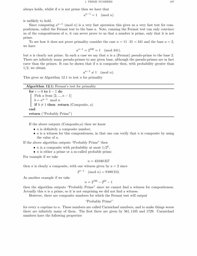
1. PRIME NUMBERS 187
always holds, whilst if n is not prime then we have that
an−1 = 1 (mod n)
is unlikely to hold.Since computing an−1 (mod n) is a very fast operation this gives us a very fast test for com-
positeness, called the Fermat test to the base a. Note, running the Fermat test can only convinceus of the compositeness of n, it can never prove to us that a number is prime, only that it is notprime.
To see how it does not prove primality consider the case n = 11 · 31 = 341 and the base a = 2,we have
an−1 = 2340 = 1 (mod 341).but n is clearly not prime. In such a case we say that n is a (Fermat) pseudo-prime to the base 2.There are infinitely many pseudo-primes to any given base, although the pseudo-primes are in factrarer than the primes. It can be shown that if n is composite then, with probability greater than1/2, we obtain
an−1 �= 1 (mod n).This gives us Algorithm 12.1 to test n for primality
Algorithm 12.1: Fermat’s test for primalityfor i = 0 to k − 1 do
Pick a from [2, ..., n − 1]b = an−1 mod nif b �= 1 then return (Composite, a)
endreturn (“Probably Prime”)
If the above outputs (Composite,a) then we know• n is definitely a composite number,• a is a witness for this compositeness, in that one can verify that n is composite by using
the value of a.If the above algorithm outputs “Probably Prime” then
• n is a composite with probability at most 1/2k,• n is either a prime or a so-called probable prime.
For example if we taken = 43040 357
then n is clearly a composite, with one witness given by a = 2 since
2n−1 (mod n) = 9 888 212.
As another example if we taken = 2192 − 264 − 1
then the algorithm outputs “Probably Prime” since we cannot find a witness for compositeness.Actually this n is a prime, so it is not surprising we did not find a witness.
However, there are composite numbers for which the Fermat test will output
“Probably Prime”
for every a coprime to n. These numbers are called Carmichael numbers, and to make things worsethere are infinitely many of them. The first three are given by 561, 1105 and 1729. Carmichaelnumbers have the following properties
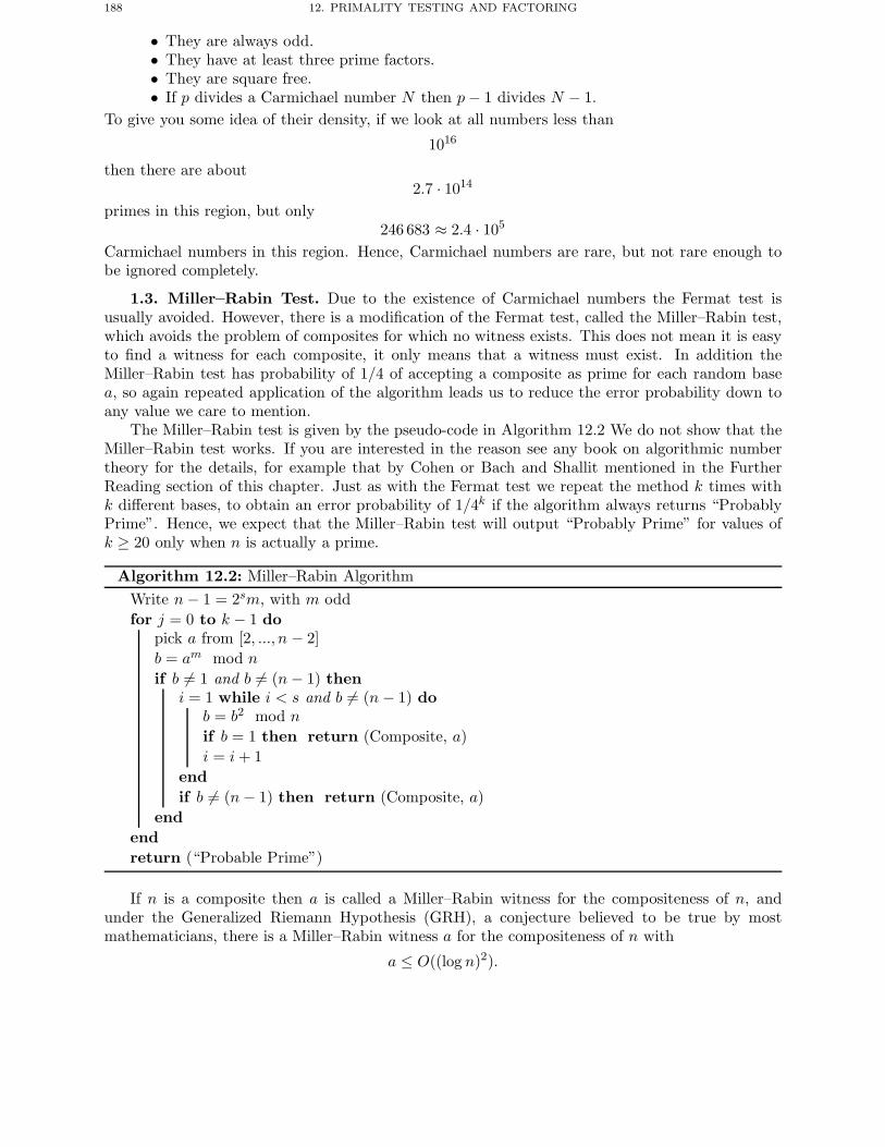
188 12. PRIMALITY TESTING AND FACTORING
• They are always odd.• They have at least three prime factors.• They are square free.• If p divides a Carmichael number N then p− 1 divides N − 1.
To give you some idea of their density, if we look at all numbers less than
1016
then there are about2.7 · 1014
primes in this region, but only246 683 ≈ 2.4 · 105
Carmichael numbers in this region. Hence, Carmichael numbers are rare, but not rare enough tobe ignored completely.
1.3. Miller–Rabin Test. Due to the existence of Carmichael numbers the Fermat test isusually avoided. However, there is a modification of the Fermat test, called the Miller–Rabin test,which avoids the problem of composites for which no witness exists. This does not mean it is easyto find a witness for each composite, it only means that a witness must exist. In addition theMiller–Rabin test has probability of 1/4 of accepting a composite as prime for each random basea, so again repeated application of the algorithm leads us to reduce the error probability down toany value we care to mention.
The Miller–Rabin test is given by the pseudo-code in Algorithm 12.2 We do not show that theMiller–Rabin test works. If you are interested in the reason see any book on algorithmic numbertheory for the details, for example that by Cohen or Bach and Shallit mentioned in the FurtherReading section of this chapter. Just as with the Fermat test we repeat the method k times withk different bases, to obtain an error probability of 1/4k if the algorithm always returns “ProbablyPrime”. Hence, we expect that the Miller–Rabin test will output “Probably Prime” for values ofk ≥ 20 only when n is actually a prime.
Algorithm 12.2: Miller–Rabin AlgorithmWrite n− 1 = 2sm, with m oddfor j = 0 to k − 1 do
pick a from [2, ..., n − 2]b = am mod nif b �= 1 and b �= (n− 1) then
i = 1 while i < s and b �= (n − 1) dob = b2 mod nif b = 1 then return (Composite, a)i = i+ 1
endif b �= (n− 1) then return (Composite, a)
endendreturn (“Probable Prime”)
If n is a composite then a is called a Miller–Rabin witness for the compositeness of n, andunder the Generalized Riemann Hypothesis (GRH), a conjecture believed to be true by mostmathematicians, there is a Miller–Rabin witness a for the compositeness of n with
a ≤ O((log n)2).
2. FACTORING ALGORITHMS 189
1.4. Primality Proofs. Up to now we have only output witnesses for compositeness, andwe can interpret such a witness as a proof of compositeness. In addition we have only obtainedprobable primes rather than numbers which are 100 percent guaranteed to be prime. In practicethis seems to be all right, since the probability of a composite number passing the Miller–Rabintest for twenty bases is around 2−40 which should never really occur in practice. But theoretically(and maybe in practice if we are totally paranoid) this could be a problem. In other words we maywant real primes and not just probable ones.
There are algorithms whose output is a witness for the primality of the number. Such a witnessis called a proof of primality. In practice such programs are only called when one is morally certainthat the number one is testing for primality is actually prime. In other words the number hasalready passed the Miller–Rabin test for a number of bases and all one now requires is a proof ofthe primality.
The most successful of these primality proving algorithms is one based on elliptic curves calledECPP (for Elliptic Curve Primality Prover). This itself is based on an older primality provingalgorithm based on finite fields due to Pocklington and Lehmer, the elliptic curve variant is due toGoldwasser and Kilian. The ECPP algorithm is a randomized algorithm which is not mathemati-cally guaranteed to always produce an output, i.e. a witness, when the input is a prime number. Ifthe input is composite then the algorithm is not guaranteed to terminate at all. Although ECPPruns in polynomial time, i.e. it is quite efficient, the proofs of primality it produces can be verifiedeven faster.
There is an algorithm due to Adleman and Huang which, unlike the ECPP method, is guar-anteed to terminate with a proof of primality on input of a prime number. It is based on ageneralization of elliptic curves called hyperelliptic curves and has never to my knowledge beenimplemented. The fact that it has never been implemented is not only due to the far more com-plicated mathematics involved, but is also due to the fact that while the hyperelliptic variant ismathematically guaranteed to produce a proof, the ECPP method will always do so in practice forless work effort.
2. Factoring Algorithms
Factoring methods are usually divided into Dark Age methods such as• Trial division,• p− 1 method,• p+ 1 method,• Pollard rho method,
and modern methods• Continued Fraction Method (CFRAC),• Quadratic Sieve (QS),• Elliptic Curve Method (ECM),• Number Field Sieve (NFS).
We do not have the time or space to discuss all of these in detail so we shall look at a couple ofDark Age methods and explain the main ideas behind some of the modern methods.
Modern factoring algorithms lie somewhere between polynomial and exponential time, in anarea called sub-exponential time. These algorithms have complexity measured by the function
LN (α, β) = exp((β + o(1))(logN)α(log logN)1−α
).
Notice that• LN (0, β) = (logN)β+o(1), i.e. polynomial time,• LN (1, β) = Nβ+o(1), i.e. exponential time.
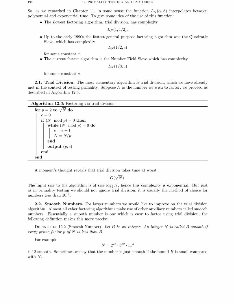
190 12. PRIMALITY TESTING AND FACTORING
So, as we remarked in Chapter 11, in some sense the function LN (α, β) interpolates betweenpolynomial and exponential time. To give some idea of the use of this function:
• The slowest factoring algorithm, trial division, has complexity
LN (1, 1/2).
• Up to the early 1990s the fastest general purpose factoring algorithm was the QuadraticSieve, which has complexity
LN (1/2, c)
for some constant c.• The current fastest algorithm is the Number Field Sieve which has complexity
LN (1/3, c)
for some constant c.
2.1. Trial Division. The most elementary algorithm is trial division, which we have alreadymet in the context of testing primality. Suppose N is the number we wish to factor, we proceed asdescribed in Algorithm 12.3.
Algorithm 12.3: Factoring via trial division
for p = 2 to√N do
e = 0if (N mod p) = 0 then
while (N mod p) = 0 doe = e+ 1N = N/p
endoutput (p, e)
endend
A moment’s thought reveals that trial division takes time at worst
O(√N).
The input size to the algorithm is of size log2N , hence this complexity is exponential. But justas in primality testing we should not ignore trial division, it is usually the method of choice fornumbers less than 1012.
2.2. Smooth Numbers. For larger numbers we would like to improve on the trial divisionalgorithm. Almost all other factoring algorithms make use of other auxiliary numbers called smoothnumbers. Essentially a smooth number is one which is easy to factor using trial division, thefollowing definition makes this more precise.
Definition 12.2 (Smooth Number). Let B be an integer. An integer N is called B-smooth ifevery prime factor p of N is less than B.
For exampleN = 278 · 389 · 113
is 12-smooth. Sometimes we say that the number is just smooth if the bound B is small comparedwith N .
2. FACTORING ALGORITHMS 191
The number of y-smooth numbers which are less than x is given by the function ψ(x, y). Thisis a rather complicated function which is approximated by
ψ(x, y) ≈ xρ(u)
where ρ is the Dickman–de Bruijn function and
u =log xlog y
.
The Dickman–de Bruijn function ρ is defined as the function which satisfies the following differential-delay equation
uρ′(u) + ρ(u− 1) = 0
for u > 1. In practice we approximate ρ(u) via the expression
ρ(u) ≈ u−u
which holds as u→ ∞. This leads to the following result, which is important in analysing advancedfactoring algorithms.
Theorem 12.3. The proportion of integers less than x, which are x1/u-smooth, is asymptoticallyequal to u−u.
Now if we sety = LN (α, β)
then
u =logNlog y
=1β
(logN
log logN
)1−α.
Hence, one can show
1Nψ(N, y) ≈ u−u
= exp(−u log u)
≈ 1LN (1 − α, γ)
,
for some constant γ. Suppose we are looking for numbers less than N which are LN (α, β)-smooth.The probability that any number less thanN is actually LN (α, β)-smooth is given by 1/LN (1−α, γ).This hopefully will explain intuitively why some of the modern method complexity estimates forfactoring are around LN (0.5, c), since to balance the smoothness bound against the probabilityestimate we take α = 1
2 . The number field sieve obtains a better complexity estimate only by usinga more mathematically complex algorithm.
We shall also require, in discussing our next factoring algorithm, the notion of a number beingB-power smooth:
Definition 12.4 (Power Smooth). A number is said to be B-power smooth if every prime powerdividing N is less than B.
For exampleN = 25 · 33
is 33-power smooth.
192 12. PRIMALITY TESTING AND FACTORING
2.3. Pollard’s P − 1 Method. The most famous name in factoring algorithms in the late20th century was John Pollard. Almost all the important advances in factoring were made by him,for example
• the P − 1 method,• the Rho-method,• the Number Field Sieve.
In this section we discuss the P − 1 method and in a later section we consider the Number FieldSieve method, the other methods we leave for the exercises at the end of the chapter.
Suppose the number we wish to factor is given by
N = p · q.In addition suppose we know (by some pure guess) an integer B such that p−1 is B-power smooth,but that q − 1 is not B-power smooth. We can then hope that p − 1 divides B!, but that q − 1 isunlikely to divide B!.
Suppose that we computea = 2B! (mod N).
Imagine that we could compute this modulo p and modulo q, we would then have
a ≡ 1 (mod p),
since• p− 1 divides B!,• ap−1 = 1 (mod p) by Fermat’s Little Theorem.
But it is unlikely that we would have
a ≡ 1 (mod q).
Hence,• p will divide a− 1,• q will not divide a− 1.
We can then recover p by computing
p = gcd(a− 1,N ),
as in Algorithm 12.4
Algorithm 12.4: Pollard’s P − 1 factoring methoda = 2for j = 2 to B do
a = aj mod Nendp = gcd(a− 1, N)if p �= 1 and p �= N then return (“p is a factor of N”)else return (“No Result”)
As an example, suppose we wish to factor
N = 15770 708 441.
We take B = 180 and running the above algorithm we obtain
a = 2B! (mod N) = 1 162 022 425.
Then we obtainp = gcd(a− 1,N) = 135 979.
2. FACTORING ALGORITHMS 193
To see why this works in this example we see that the prime factorization of N is given by
N = 135 979 · 115 979
and we have
p− 1 = 135 978 − 1 = 2 · 3 · 131 · 173,q − 1 = 115 978 − 1 = 2 · 103 · 563.
Hence p− 1 is indeed B-power smooth, whilst q − 1 is not B-power smooth.One can show that the complexity of the P − 1 method is given by
O(B logB(logN)2 + (logN)3).
So if we choose B = O((logN)i), for some integer i, then this is a polynomial-time factoringalgorithm, but it only works for numbers of a special form.
Due to the P − 1 method one often sees recommended that RSA primes are chosen to satisfy
p− 1 = 2p1 and q − 1 = 2q1,
where p1 and q1 are both primes. In this situation the primes p and q are called safe primes. How-ever, this is not really needed these days with the large RSA moduli we use in current applications.This is because the probability that for a random 512-bit prime p, the number p − 1 is B-powersmooth for a small value of B is very small. Hence, choosing random 512-bit primes would in alllikelihood render the P − 1 method useless.
2.4. Difference of Two Squares. A basic trick in factoring algorithms, known for manycenturies, is to produce two numbers x and y, of around the same size as N , such that
x2 = y2 (mod N).
Since then we have
x2 − y2 = (x− y)(x+ y) = 0 (mod N).
If N = p · q then we have four possible cases
(1) p divides x− y and q divides x+ y.(2) p divides x+ y and q divides x− y.(3) p and q both divide x− y but neither divide x+ y.(4) p and q both divide x+ y but neither divide x− y.
All these cases can occur with equal probability, namely 14 . If we then compute
d = gcd(x− y,N),
our previous four cases then divide into the cases
(1) d = p.(2) d = q.(3) d = N .(4) d = 1.
Since all these cases occur with equal probability, we see that with probability 12 we will obtain a
non-trivial factor of N . The only problem is, how do we find x and y such that x2 = y2 (mod N)?
194 12. PRIMALITY TESTING AND FACTORING
3. Modern Factoring Methods
Most modern factoring methods have the following strategy based on the difference of twosquares method described at the end of the last section.
• Take a smoothness bound B.• Compute a factorbase F of all prime numbers p less than B.• Find a large number of values of x and y, such that x and y are B-smooth and
x = y (mod N).
These are called relations on the factorbase.• Using linear algebra modulo 2, find a combination of the relations to give an X and Y
withX2 = Y 2 (mod N).
• Attempt to factor N by computing gcd(X − Y,N).The trick in all algorithms of this form is how to find the relations. All the other details of thealgorithms are basically the same. Such a strategy can also be used to solve discrete logarithmproblems as well, which we shall discuss in a later chapter. In this section we explain the parts ofthe modern factoring algorithms which are common and justify why they work.
One way of looking at such algorithms is in the context of computational group theory. We havealready shown that knowing the order of the group (Z/NZ)∗, for an RSA modulus N , is the sameas knowing the prime factors of N . Hence, the problem is really one of computing a group order.The factorbase is essentially a set of generators of the group (Z/NZ)∗, whilst the relations arerelations between the generators of this group. Once a sufficiently large number of relations havebeen found then, since the group is a finite abelian group, standard group theoretic algorithms willcompute the group structure and hence the group order. These general group theoretic algorithmscould include computing the Smith Normal Form of the associated matrix. Hence, it should notbe surprising that linear algebra is used on the relations so as to factor the integer N .
3.1. Combining Relations. The Smith Normal Form algorithm is far too complicated forfactoring algorithms where a more elementary approach, still based on linear algebra, can be used,as we shall now explain. Suppose we have the relations
p2q5r2 = p3q4r3 (mod N),
pq3r5 = pqr2 (mod N),
p3q5r3 = pq3r2 (mod N),
where p, q and r are primes in our factorbase, F = {p, q, r}. Dividing one side by the other in eachof our relations we obtain
p−1qr−1 = 1 (mod N),
q2r3 = 1 (mod N),
p2q2r = 1 (mod N).
Multiplying the last two equations together we obtain
p0+2q2+2r3+1 ≡ 1 (mod N).
In other wordsp2q4r4 ≡ 1 (mod N).
Hence if X = pq2r2 and Y = 1 then we obtain
X2 = Y 2 (mod N)
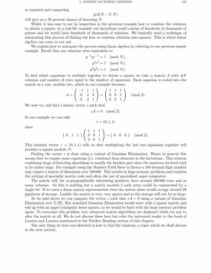
3. MODERN FACTORING METHODS 195
as required and computinggcd(X − Y,N)
will give us a 50 percent chance of factoring N .Whilst it was easy to see by inspection in the previous example how to combine the relations
to obtain a square, in a real-life example our factorbase could consist of hundreds of thousands ofprimes and we would have hundreds of thousands of relations. We basically need a technique ofautomating this process of finding out how to combine relations into squares. This is where linearalgebra can come to our aid.
We explain how to automate the process using linear algebra by referring to our previous simpleexample. Recall that our relations were equivalent to
p−1qr−1 = 1 (mod N),
q2r3 = 1 (mod N),
p2q2r = 1 (mod N).
To find which equations to multiply together to obtain a square we take a matrix A with #Fcolumns and number of rows equal to the number of equations. Each equation is coded into thematrix as a row, modulo two, which in our example becomes
A =
⎛⎝ −1 1 1
0 2 32 2 1
⎞⎠ =
⎛⎝ 1 1 1
0 0 10 0 1
⎞⎠ (mod 2).
We now try and find a binary vector z such that
zA = 0 (mod 2).
In our example we can takez = (0, 1, 1)
since (0 1 1
)⎛⎝ 1 1 10 0 10 0 1
⎞⎠ =(
0 0 0)
(mod 2).
This solution vector z = (0, 1, 1) tells us that multiplying the last two equations together willproduce a square modulo N .
Finding the vector z is done using a variant of Gaussian Elimination. Hence in general thismeans that we require more equations (i.e. relations) than elements in the factorbase. This relationcombining stage of factoring algorithms is usually the hardest part since the matrices involved tendto be rather large. For example using the Number Field Sieve to factor a 100 decimal digit numbermay require a matrix of dimension over 100 000. This results in huge memory problems and requiresthe writing of specialist matrix code and often the use of specialized super computers.
The matrix will, for cryptographically interesting numbers, have around 500 000 rows and asmany columns. As this is nothing but a matrix modulo 2 each entry could be represented by asingle bit. If we used a dense matrix representation then the matrix alone would occupy around 29gigabytes of storage. Luckily the matrix is very, very sparse and so the storage will not be so large.
As we said above we can compute the vector z such that zA = 0 using a variant of GaussianElimination over Z/2Z. But standard Gaussian Elimination would start with a sparse matrix andend up with an upper triangular dense matrix, so we would be back with the huge memory problemagain. To overcome this problem very advanced matrix algorithms are deployed which try not toalter the matrix at all. We do not discuss these here but refer the interested reader to the book ofLenstra and Lenstra mentioned in the Further Reading section of this chapter.
The only thing we have not sketched is how to find the relations, a topic which we shall discussin the next section.
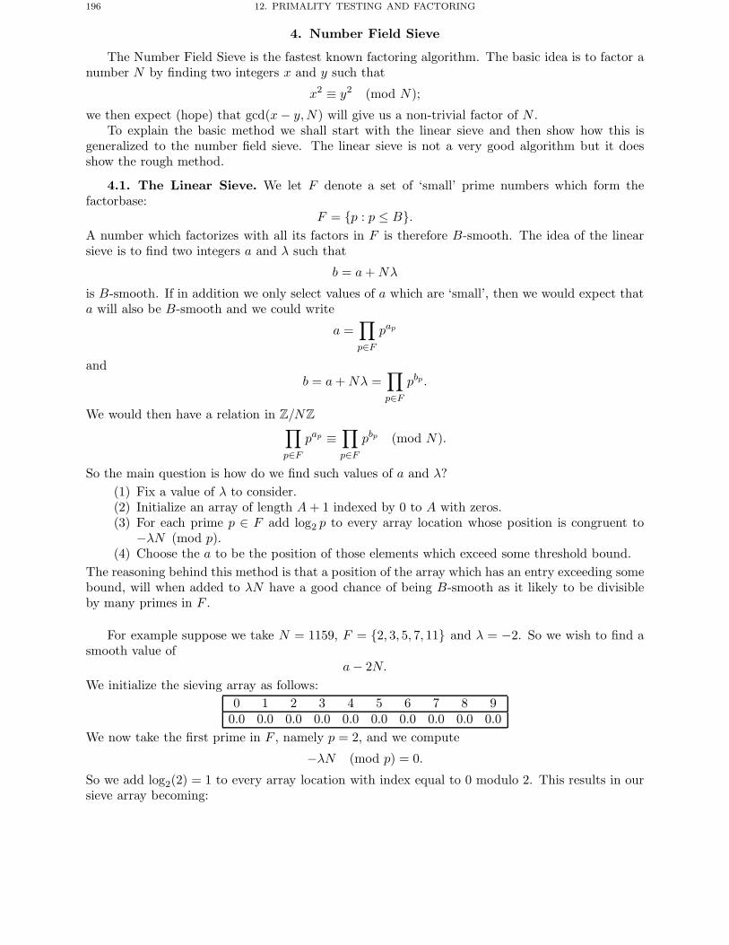
196 12. PRIMALITY TESTING AND FACTORING
4. Number Field Sieve
The Number Field Sieve is the fastest known factoring algorithm. The basic idea is to factor anumber N by finding two integers x and y such that
x2 ≡ y2 (mod N);
we then expect (hope) that gcd(x− y,N) will give us a non-trivial factor of N .To explain the basic method we shall start with the linear sieve and then show how this is
generalized to the number field sieve. The linear sieve is not a very good algorithm but it doesshow the rough method.
4.1. The Linear Sieve. We let F denote a set of ‘small’ prime numbers which form thefactorbase:
F = {p : p ≤ B}.A number which factorizes with all its factors in F is therefore B-smooth. The idea of the linearsieve is to find two integers a and λ such that
b = a+Nλ
is B-smooth. If in addition we only select values of a which are ‘small’, then we would expect thata will also be B-smooth and we could write
a =∏p∈F
pap
andb = a+Nλ =
∏p∈F
pbp .
We would then have a relation in Z/NZ∏p∈F
pap ≡∏p∈F
pbp (mod N).
So the main question is how do we find such values of a and λ?(1) Fix a value of λ to consider.(2) Initialize an array of length A+ 1 indexed by 0 to A with zeros.(3) For each prime p ∈ F add log2 p to every array location whose position is congruent to
−λN (mod p).(4) Choose the a to be the position of those elements which exceed some threshold bound.
The reasoning behind this method is that a position of the array which has an entry exceeding somebound, will when added to λN have a good chance of being B-smooth as it likely to be divisibleby many primes in F .
For example suppose we take N = 1159, F = {2, 3, 5, 7, 11} and λ = −2. So we wish to find asmooth value of
a− 2N.We initialize the sieving array as follows:
0 1 2 3 4 5 6 7 8 90.0 0.0 0.0 0.0 0.0 0.0 0.0 0.0 0.0 0.0
We now take the first prime in F , namely p = 2, and we compute
−λN (mod p) = 0.
So we add log2(2) = 1 to every array location with index equal to 0 modulo 2. This results in oursieve array becoming:
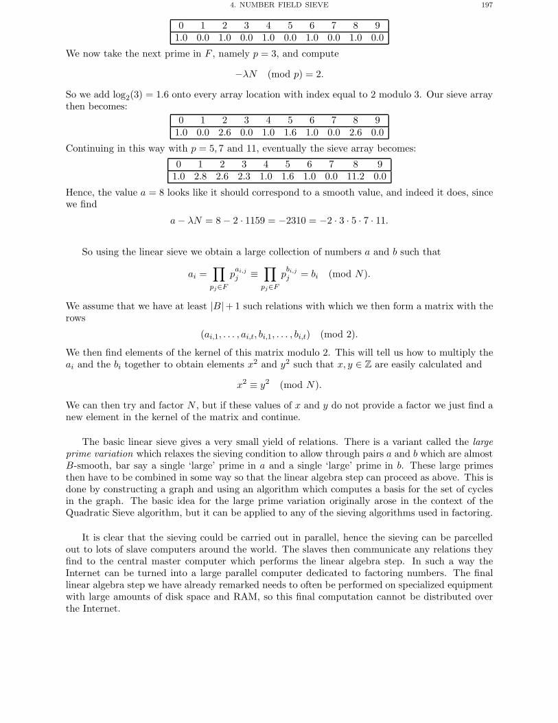
4. NUMBER FIELD SIEVE 197
0 1 2 3 4 5 6 7 8 91.0 0.0 1.0 0.0 1.0 0.0 1.0 0.0 1.0 0.0
We now take the next prime in F , namely p = 3, and compute
−λN (mod p) = 2.
So we add log2(3) = 1.6 onto every array location with index equal to 2 modulo 3. Our sieve arraythen becomes:
0 1 2 3 4 5 6 7 8 91.0 0.0 2.6 0.0 1.0 1.6 1.0 0.0 2.6 0.0
Continuing in this way with p = 5, 7 and 11, eventually the sieve array becomes:
0 1 2 3 4 5 6 7 8 91.0 2.8 2.6 2.3 1.0 1.6 1.0 0.0 11.2 0.0
Hence, the value a = 8 looks like it should correspond to a smooth value, and indeed it does, sincewe find
a− λN = 8 − 2 · 1159 = −2310 = −2 · 3 · 5 · 7 · 11.
So using the linear sieve we obtain a large collection of numbers a and b such that
ai =∏pj∈F
pai,jj ≡
∏pj∈F
pbi,jj = bi (mod N).
We assume that we have at least |B|+ 1 such relations with which we then form a matrix with therows
(ai,1, . . . , ai,t, bi,1, . . . , bi,t) (mod 2).
We then find elements of the kernel of this matrix modulo 2. This will tell us how to multiply theai and the bi together to obtain elements x2 and y2 such that x, y ∈ Z are easily calculated and
x2 ≡ y2 (mod N).
We can then try and factor N , but if these values of x and y do not provide a factor we just find anew element in the kernel of the matrix and continue.
The basic linear sieve gives a very small yield of relations. There is a variant called the largeprime variation which relaxes the sieving condition to allow through pairs a and b which are almostB-smooth, bar say a single ‘large’ prime in a and a single ‘large’ prime in b. These large primesthen have to be combined in some way so that the linear algebra step can proceed as above. This isdone by constructing a graph and using an algorithm which computes a basis for the set of cyclesin the graph. The basic idea for the large prime variation originally arose in the context of theQuadratic Sieve algorithm, but it can be applied to any of the sieving algorithms used in factoring.
It is clear that the sieving could be carried out in parallel, hence the sieving can be parcelledout to lots of slave computers around the world. The slaves then communicate any relations theyfind to the central master computer which performs the linear algebra step. In such a way theInternet can be turned into a large parallel computer dedicated to factoring numbers. The finallinear algebra step we have already remarked needs to often be performed on specialized equipmentwith large amounts of disk space and RAM, so this final computation cannot be distributed overthe Internet.
198 12. PRIMALITY TESTING AND FACTORING
4.2. The Number Field Sieve. The linear sieve is simply not good enough to factor largenumbers. Indeed the linear sieve was never proposed as a real factoring algorithm, its operation ishowever instructive for other algorithms of this type. The number field sieve uses the arithmetic ofalgebraic number fields to construct the desired relations between the elements of the factorbase.All that changes is the way the relations are found. The linear algebra step, the large primevariations and the slave/master approach all go over to NFS virtually unchanged. We now explainthe NFS, but in a much simpler form than is actually used in real-life so as to aid the exposition.Those readers who do not know any algebraic number theory may wish to skip this section.
First we construct two monic, irreducible polynomials with integer coefficients f1 and f2, ofdegree d1 and d2 respectively, such that there exists an m ∈ Z such that
f1(m) ≡ f2(m) ≡ 0 (mod N).
The number field sieve will make use of arithmetic in the number fields K1 and K2 given by
K1 = Q(θ1) and K2 = Q(θ2),
where θ1 and θ2 are defined by f1(θ1) = f2(θ2) = 0. We then have two homomorphisms φ1 and φ2
given by
φi :{
Z[θi] −→ Z/NZ
θi −→ m.
We aim to use a sieve, just as in the linear sieve, to find a set
S ⊂ {(a, b) ∈ Z2 : gcd(a, b) = 1}such that ∏
S
(a− bθ1) = β2
and ∏S
(a− bθ2) = γ2,
where β ∈ K1 and γ ∈ K2. If we found two such values of β and γ then we would have
φ1(β)2 ≡ φ2(γ)2 (mod N)
and hopefullygcd(N,φ1(β) − φ2(γ))
would be a factor of N .This leads to three obvious problems
• How do we find the set S?• Given β2 ∈ Q[θ1], how do we compute β?• How do we find the polynomials f1 and f2 in the first place?
4.2.1. How do we find the set S?: Similar to the linear sieve we can find such a set S usinglinear algebra provided we can find lots of a and b such that
a− bθ1 and a− bθ2
are both ‘smooth’. But what does it mean for these two objects to be smooth? It is here that thetheory of algebraic number fields comes in, by generalizing our earlier definition of smooth integersto algebraic integers we obtain the definition:
Definition 12.5. An algebraic integer is ‘smooth’ if and only if the ideal it generates is onlydivisible by ‘small’ prime ideals.
4. NUMBER FIELD SIEVE 199
Define Fi(X,Y ) = Y difi(X/Y ) then
NQ(θi)/Q(a− bθi) = Fi(a, b).
We define two factorbases, one for each of the polynomials
Fi = {(p, r) : p a prime, r ∈ Z such that fi(r) ≡ 0 (mod p)} .Each element of Fi corresponds to a degree one prime ideal of Z[θi], which is a sub-order of thering of integers of OQ(θi), given by
〈p, θi − r〉 = pZ[θi] + (θi − r)Z[θi].
Given values of a and b we can easily determine whether the ideal 〈a− θib〉 ‘factorizes’ over ourfactorbase. Note factorizes is in quotes as unique factorization of ideals may not hold in Z[θi],whilst it will hold in OQ(θi). It will turn out that this is not really a problem. To see why this isnot a problem you should consult the book by Lenstra and Lenstra.
If Z[θi] = OQ(θi) then the following method does indeed give the unique prime ideal factorizationof 〈a− θib〉.
• Write
Fi(a, b) =∏
(pj ,r)∈Fips(i)j
j .
• We have (a : b) = (r : 1) (mod p), as an element in the projective space of dimension oneover Fp, if the ideal corresponding to (p, r) is included in a non-trivial way in the idealfactorization of a− θib.
• We have
〈a− θib〉 =∏
(pj ,r)∈Fi〈pj , θi − r〉s(i)j .
This leads to the following algorithm to sieve for values of a and b, such that 〈a− θib〉 is an idealwhich factorizes over the factorbase. Just as with the linear sieve, the use of sieving allows us toavoid lots of expensive trial divisions when trying to determine smooth ideals. We end up onlyperforming factorizations where we already know we have a good chance of being successful.
• Fix a.• Initialize the sieve array for −B ≤ b ≤ B by
S[b] = log2(F1(a, b) · F2(a, b)).
• For every (p, r) ∈ Fi subtract log2 p from every array element such that
a− rb ≡ 0 (mod p).
• The bs we want are the ones such that S[b] lies below some tolerance level.If the tolerance level is set in a sensible way then we have a good chance that both F1(a, b) andF2(a, b) factor over the prime ideals in the factorbase, with the possibility of some large prime idealscreeping in. We keep these factorizations as a relation, just as we did with the linear sieve.
Then, after some linear algebra, we can find a subset S of all the pairs (a, b) we have foundsuch that ∏
(a,b)∈S〈a− bθi〉 = square of an ideal in Z[θi].
This is not however good enough, recall we want the product∏a − bθi to be the square of an
element of Z[θi]. To overcome this problem we need to add information from the ‘infinite’ places.This is done by adding in some quadratic characters, an idea introduced by Adleman. Let q be
200 12. PRIMALITY TESTING AND FACTORING
a rational prime (in neither F1 nor F2) such that there is an sq with fi(sq) ≡ 0 (mod q) andf ′i(sq) �≡ 0 (mod q) for either i = 1 or i = 2. Then our extra condition is that we require
∏(a,b)∈S
(a− bsqq
)= 1,
where ( .q ) denotes the Legendre symbol. As the Legendre symbol is multiplicative this gives us anextra condition to put into our matrix. We need to add this condition for a number of primes q,hence we choose a set of such primes q and put the associated characters into our matrix as anextra column of 0s or 1s corresponding to:
if(a− bsqq
)={
1 then enter 0,−1 then enter 1.
So after finding enough relations we hope to be able to find a subset S such that hopefully∏S
(a− bθ1) = β2 and∏S
(a− bθ2) = γ2.
4.2.2. How do we take the square roots?: We then need to be able to take the square root ofβ2 to recover β, and similarly for γ2. Each β2 is given in the form
β2 =d1−1∑j=0
ajθj1
where the aj are huge integers. We want to be able to determine the solutions bj ∈ Z to theequation ⎛
⎝d1−1∑j=0
bjθj1
⎞⎠
2
=d1−1∑j=0
ajθj1.
One way this is overcome, due to Couveignes, is by computing such a square root modulo a largenumber of very, very large primes p. We then perform Hensel lifting and Chinese remainderingto hopefully recover our square root. This is the easiest method to understand although moreadvanced methods are available, such as that by Nguyen.
4.2.3. Choosing the initial polynomials: This is the part of the method that is a black art atthe moment. We require only the following conditions to be met
f1(m) ≡ f2(m) ≡ 0 (mod N).
However there are good heuristic reasons why it also might be desirable to construct polynomialswith additional properties such as
• The polynomials have small coefficients.• f1 and f2 have ‘many’ real roots. Note, a random polynomial probably would have no real
roots on average.• f1 and f2 have ‘many’ roots modulo lots of small prime numbers.• The Galois groups of f1 and f2 are ‘small’
It is often worth spending a few weeks trying to find a good couple of polynomials before one startsto attempt the factorization algorithm proper. There are a number of search strategies used forfinding these polynomials. Once a few candidates are found some experimental sieving is performedto see which appear to be the most successful, in that they yield the most relations. Then once adecision has been made one can launch the sieving stage ‘for real’.
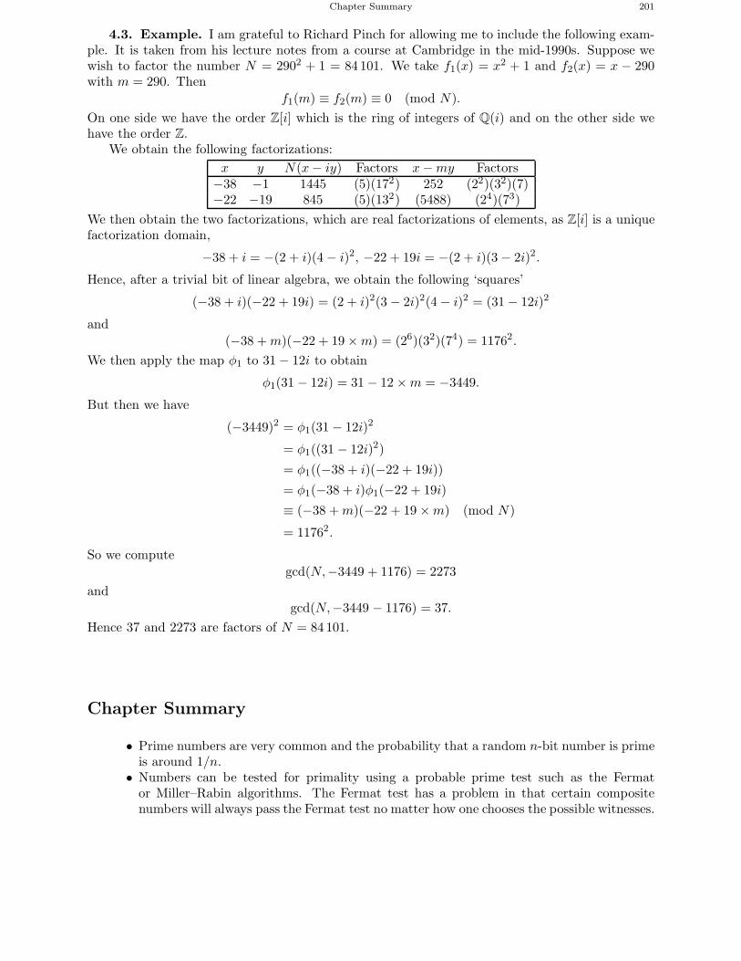
Chapter Summary 201
4.3. Example. I am grateful to Richard Pinch for allowing me to include the following exam-ple. It is taken from his lecture notes from a course at Cambridge in the mid-1990s. Suppose wewish to factor the number N = 2902 + 1 = 84 101. We take f1(x) = x2 + 1 and f2(x) = x − 290with m = 290. Then
f1(m) ≡ f2(m) ≡ 0 (mod N).On one side we have the order Z[i] which is the ring of integers of Q(i) and on the other side wehave the order Z.
We obtain the following factorizations:x y N(x− iy) Factors x−my Factors
−38 −1 1445 (5)(172) 252 (22)(32)(7)−22 −19 845 (5)(132) (5488) (24)(73)
We then obtain the two factorizations, which are real factorizations of elements, as Z[i] is a uniquefactorization domain,
−38 + i = −(2 + i)(4 − i)2, −22 + 19i = −(2 + i)(3 − 2i)2.
Hence, after a trivial bit of linear algebra, we obtain the following ‘squares’
(−38 + i)(−22 + 19i) = (2 + i)2(3 − 2i)2(4 − i)2 = (31 − 12i)2
and(−38 +m)(−22 + 19 ×m) = (26)(32)(74) = 11762.
We then apply the map φ1 to 31 − 12i to obtain
φ1(31 − 12i) = 31 − 12 ×m = −3449.
But then we have
(−3449)2 = φ1(31 − 12i)2
= φ1((31 − 12i)2)
= φ1((−38 + i)(−22 + 19i))
= φ1(−38 + i)φ1(−22 + 19i)
≡ (−38 +m)(−22 + 19 ×m) (mod N)
= 11762.
So we computegcd(N,−3449 + 1176) = 2273
andgcd(N,−3449 − 1176) = 37.
Hence 37 and 2273 are factors of N = 84101.
Chapter Summary
• Prime numbers are very common and the probability that a random n-bit number is primeis around 1/n.
• Numbers can be tested for primality using a probable prime test such as the Fermator Miller–Rabin algorithms. The Fermat test has a problem in that certain compositenumbers will always pass the Fermat test no matter how one chooses the possible witnesses.
202 12. PRIMALITY TESTING AND FACTORING
• If one really needs to be certain that a number is prime then there are primality provingalgorithms which run in polynomial time.
• Factoring algorithms are often based on the problem of finding the difference of twosquares.
• Modern factoring algorithms run in two stages: In the first stage one collects a lot of rela-tions on a factorbase by using a process called sieving, which can be done using thousandsof computers on the Internet. In the second stage these relations are processed using linearalgebra on a big central server. The final factorization is obtained by finding a differenceof two squares.
Further Reading
The definitive reference work on computational number theory which deals with many algo-rithms for factoring and primality proving is the book by Cohen. The book by Bach and Shallitalso provides a good reference for primality testing. The main book explaining the Number FieldSieve is the book by Lenstra and Lenstra.
E. Bach and J. Shallit. Algorithmic Number Theory. Volume 1: Efficient Algorithms. MIT Press,1996.
H. Cohen. A Course in Computational Algebraic Number Theory. Springer-Verlag, 1993.
A. Lenstra and H. Lenstra. The Development of the Number Field Sieve. Springer-Verlag, 1993.
CHAPTER 13
Discrete Logarithms
Chapter Goals
• To examine algorithms for solving the discrete logarithm problem.• To introduce the Pohlig–Hellman algorithm.• To introduce the Baby-Step/Giant-Step algorithm.• To explain the methods of Pollard.• To show how discrete logarithms can be solved in finite fields using algorithms like those
used for factoring.• To describe the known results on the elliptic curve discrete logarithm problem.
1. Introduction
In this chapter we survey the methods known for solving the discrete logarithm problem,
h = gx
in various groups G. These algorithms fall into one of two categories, either the algorithms aregeneric and apply to any finite abelian group or the algorithms are specific to the special groupunder consideration.
We start with general purpose algorithms and then move onto special purpose algorithms laterin the chapter.
2. Pohlig–Hellman
The first observation to make is that the discrete logarithm problem in a group G is only as hardas the discrete logarithm problem in the largest subgroup of prime order in G. This observation isdue to Pohlig and Hellman, and it applies in an arbitrary finite abelian group.
To explain the Pohlig–Hellman algorithm, suppose we have a finite cyclic abelian group G = 〈g〉whose order is given by
N = #G =t∏i=1
peii .
Now suppose we are given h ∈ 〈g〉, so there exists an integer x such that
h = gx.
Our aim is to find x by first finding it modulo peii and then using the Chinese Remainder Theoremto recover it modulo N .
From basic group theory we know that there is a group isomorphism
φ : G −→ Cpe11× · · · × Cpett
,
203
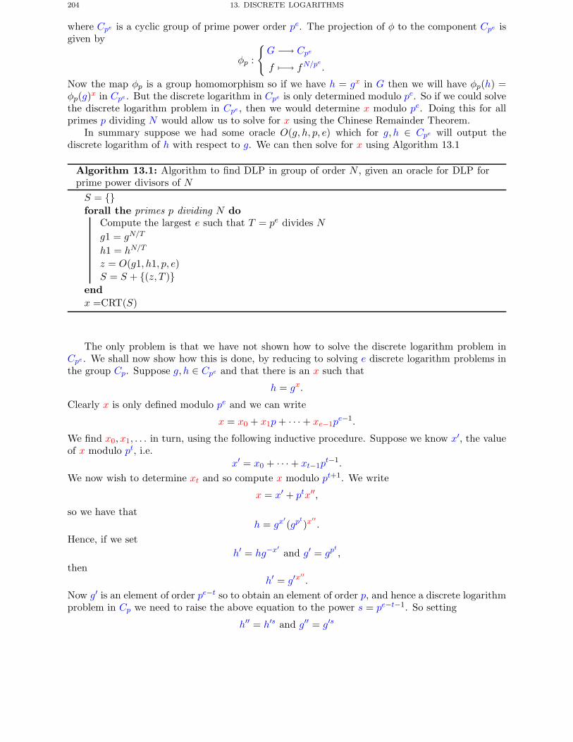
204 13. DISCRETE LOGARITHMS
where Cpe is a cyclic group of prime power order pe. The projection of φ to the component Cpe isgiven by
φp :
{G −→ Cpe
f −→ fN/pe.
Now the map φp is a group homomorphism so if we have h = gx in G then we will have φp(h) =φp(g)x in Cpe . But the discrete logarithm in Cpe is only determined modulo pe. So if we could solvethe discrete logarithm problem in Cpe , then we would determine x modulo pe. Doing this for allprimes p dividing N would allow us to solve for x using the Chinese Remainder Theorem.
In summary suppose we had some oracle O(g, h, p, e) which for g, h ∈ Cpe will output thediscrete logarithm of h with respect to g. We can then solve for x using Algorithm 13.1
Algorithm 13.1: Algorithm to find DLP in group of order N , given an oracle for DLP forprime power divisors of NS = {}forall the primes p dividing N do
Compute the largest e such that T = pe divides Ng1 = gN/T
h1 = hN/T
z = O(g1, h1, p, e)S = S + {(z, T )}
endx =CRT(S)
The only problem is that we have not shown how to solve the discrete logarithm problem inCpe . We shall now show how this is done, by reducing to solving e discrete logarithm problems inthe group Cp. Suppose g, h ∈ Cpe and that there is an x such that
h = gx.
Clearly x is only defined modulo pe and we can write
x = x0 + x1p+ · · · + xe−1pe−1.
We find x0, x1, . . . in turn, using the following inductive procedure. Suppose we know x′, the valueof x modulo pt, i.e.
x′ = x0 + · · · + xt−1pt−1.
We now wish to determine xt and so compute x modulo pt+1. We write
x = x′ + ptx′′,
so we have thath = gx
′(gp
t)x
′′.
Hence, if we seth′ = hg−x
′and g′ = gp
t,
thenh′ = g′x
′′.
Now g′ is an element of order pe−t so to obtain an element of order p, and hence a discrete logarithmproblem in Cp we need to raise the above equation to the power s = pe−t−1. So setting
h′′ = h′s and g′′ = g′s
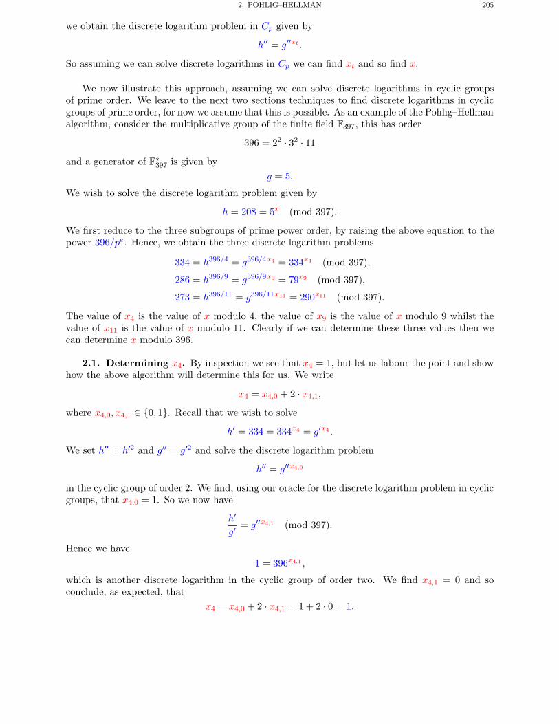
2. POHLIG–HELLMAN 205
we obtain the discrete logarithm problem in Cp given by
h′′ = g′′xt .
So assuming we can solve discrete logarithms in Cp we can find xt and so find x.
We now illustrate this approach, assuming we can solve discrete logarithms in cyclic groupsof prime order. We leave to the next two sections techniques to find discrete logarithms in cyclicgroups of prime order, for now we assume that this is possible. As an example of the Pohlig–Hellmanalgorithm, consider the multiplicative group of the finite field F397, this has order
396 = 22 · 32 · 11and a generator of F∗
397 is given byg = 5.
We wish to solve the discrete logarithm problem given by
h = 208 = 5x (mod 397).
We first reduce to the three subgroups of prime power order, by raising the above equation to thepower 396/pe. Hence, we obtain the three discrete logarithm problems
334 = h396/4 = g396/4x4 = 334x4 (mod 397),
286 = h396/9 = g396/9x9 = 79x9 (mod 397),
273 = h396/11 = g396/11x11 = 290x11 (mod 397).
The value of x4 is the value of x modulo 4, the value of x9 is the value of x modulo 9 whilst thevalue of x11 is the value of x modulo 11. Clearly if we can determine these three values then wecan determine x modulo 396.
2.1. Determining x4. By inspection we see that x4 = 1, but let us labour the point and showhow the above algorithm will determine this for us. We write
x4 = x4,0 + 2 · x4,1,
where x4,0, x4,1 ∈ {0, 1}. Recall that we wish to solve
h′ = 334 = 334x4 = g′x4 .
We set h′′ = h′2 and g′′ = g′2 and solve the discrete logarithm problem
h′′ = g′′x4,0
in the cyclic group of order 2. We find, using our oracle for the discrete logarithm problem in cyclicgroups, that x4,0 = 1. So we now have
h′
g′= g′′x4,1 (mod 397).
Hence we have1 = 396x4,1 ,
which is another discrete logarithm in the cyclic group of order two. We find x4,1 = 0 and soconclude, as expected, that
x4 = x4,0 + 2 · x4,1 = 1 + 2 · 0 = 1.
206 13. DISCRETE LOGARITHMS
2.2. Determining x9. We write
x9 = x9,0 + 3 · x9,1,
where x9,0, x9,1 ∈ {0, 1, 2}. Recall that we wish to solve
h′ = 286 = 79x9 = g′x9.
We set h′′ = h′3 and g′′ = g′3 and solve the discrete logarithm problem
h′′ = 34 = g′′x9,0 = 362x9,0
in the cyclic group of order 3. We find, using our oracle for the discrete logarithm problem in cyclicgroups, that x9,0 = 2. So we now have
h′
g′2= g′′x9,1 (mod 397).
Hence we have1 = 362x9,1 ,
which is another discrete logarithm in the cyclic group of order two. We find x9,1 = 0 and soconclude that
x9 = x9,0 + 3 · x9,1 = 2 + 3 · 0 = 2.
2.3. Determining x11. We are already in a cyclic group of prime order, so applying our oracleto the discrete logarithm problem
273 = 290x11 (mod 397),
we find that x11 = 6.
So we have determined that if
208 = 5x (mod 397),
then x is given by
x = 1 (mod 4),
x = 2 (mod 9),
x = 6 (mod 11).
If we apply the Chinese Remainder Theorem to this set of three simultaneous equations then weobtain that the solution to our discrete logarithm problem is given by
x = 281.
3. Baby-Step/Giant-Step Method
In our above discussion of the Pohlig–Hellman algorithm we assumed we had an oracle to solvethe discrete logarithm problem in cyclic groups of prime order. We shall now describe a generalmethod of solving such problems due to Shanks called the Baby-Step/Giant-Step method. Onceagain this is a generic method which applies to any cyclic finite abelian group.
Since the intermediate steps in the Pohlig–Hellman algorithm are quite simple, the difficultyof solving a general discrete logarithm problem will be dominated by the time required to solvethe discrete logarithm problem in the cyclic subgroups of prime order. Hence, for generic groupsthe complexity of the Baby-Step/Giant-Step method will dominate the overall complexity of anyalgorithm. Indeed one can show that the following method is the best possible method, time-wise,for solving the discrete logarithm problem in an arbitrary group. Of course in any actual groupthere may be a special purpose algorithm which works faster, but in general the following is provablythe best one can do.
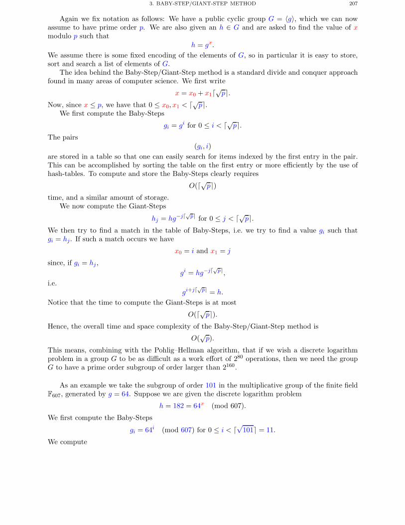
3. BABY-STEP/GIANT-STEP METHOD 207
Again we fix notation as follows: We have a public cyclic group G = 〈g〉, which we can nowassume to have prime order p. We are also given an h ∈ G and are asked to find the value of xmodulo p such that
h = gx.
We assume there is some fixed encoding of the elements of G, so in particular it is easy to store,sort and search a list of elements of G.
The idea behind the Baby-Step/Giant-Step method is a standard divide and conquer approachfound in many areas of computer science. We first write
x = x0 + x1�√p�.Now, since x ≤ p, we have that 0 ≤ x0, x1 < �√p�.
We first compute the Baby-Steps
gi = gi for 0 ≤ i < �√p�.The pairs
(gi, i)are stored in a table so that one can easily search for items indexed by the first entry in the pair.This can be accomplished by sorting the table on the first entry or more efficiently by the use ofhash-tables. To compute and store the Baby-Steps clearly requires
O(�√p�)time, and a similar amount of storage.
We now compute the Giant-Steps
hj = hg−j�√p for 0 ≤ j < �√p�.
We then try to find a match in the table of Baby-Steps, i.e. we try to find a value gi such thatgi = hj . If such a match occurs we have
x0 = i and x1 = j
since, if gi = hj ,gi = hg−j�
√p,
i.e.gi+j�
√p = h.
Notice that the time to compute the Giant-Steps is at most
O(�√p�).Hence, the overall time and space complexity of the Baby-Step/Giant-Step method is
O(√p).
This means, combining with the Pohlig–Hellman algorithm, that if we wish a discrete logarithmproblem in a group G to be as difficult as a work effort of 280 operations, then we need the groupG to have a prime order subgroup of order larger than 2160.
As an example we take the subgroup of order 101 in the multiplicative group of the finite fieldF607, generated by g = 64. Suppose we are given the discrete logarithm problem
h = 182 = 64x (mod 607).
We first compute the Baby-Steps
gi = 64i (mod 607) for 0 ≤ i < �√
101� = 11.
We compute
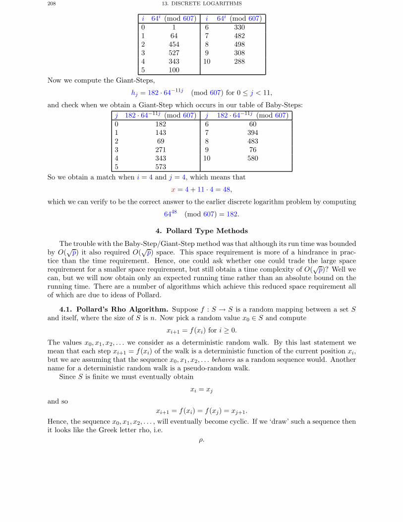
208 13. DISCRETE LOGARITHMS
i 64i (mod 607) i 64i (mod 607)0 1 6 3301 64 7 4822 454 8 4983 527 9 3084 343 10 2885 100
Now we compute the Giant-Steps,
hj = 182 · 64−11j (mod 607) for 0 ≤ j < 11,
and check when we obtain a Giant-Step which occurs in our table of Baby-Steps:j 182 · 64−11j (mod 607) j 182 · 64−11j (mod 607)0 182 6 601 143 7 3942 69 8 4833 271 9 764 343 10 5805 573
So we obtain a match when i = 4 and j = 4, which means that
x = 4 + 11 · 4 = 48,
which we can verify to be the correct answer to the earlier discrete logarithm problem by computing
6448 (mod 607) = 182.
4. Pollard Type Methods
The trouble with the Baby-Step/Giant-Step method was that although its run time was boundedby O(
√p) it also required O(
√p) space. This space requirement is more of a hindrance in prac-
tice than the time requirement. Hence, one could ask whether one could trade the large spacerequirement for a smaller space requirement, but still obtain a time complexity of O(
√p)? Well we
can, but we will now obtain only an expected running time rather than an absolute bound on therunning time. There are a number of algorithms which achieve this reduced space requirement allof which are due to ideas of Pollard.
4.1. Pollard’s Rho Algorithm. Suppose f : S → S is a random mapping between a set Sand itself, where the size of S is n. Now pick a random value x0 ∈ S and compute
xi+1 = f(xi) for i ≥ 0.
The values x0, x1, x2, . . . we consider as a deterministic random walk. By this last statement wemean that each step xi+1 = f(xi) of the walk is a deterministic function of the current position xi,but we are assuming that the sequence x0, x1, x2, . . . behaves as a random sequence would. Anothername for a deterministic random walk is a pseudo-random walk.
Since S is finite we must eventually obtain
xi = xj
and soxi+1 = f(xi) = f(xj) = xj+1.
Hence, the sequence x0, x1, x2, . . . , will eventually become cyclic. If we ‘draw’ such a sequence thenit looks like the Greek letter rho, i.e.
ρ.
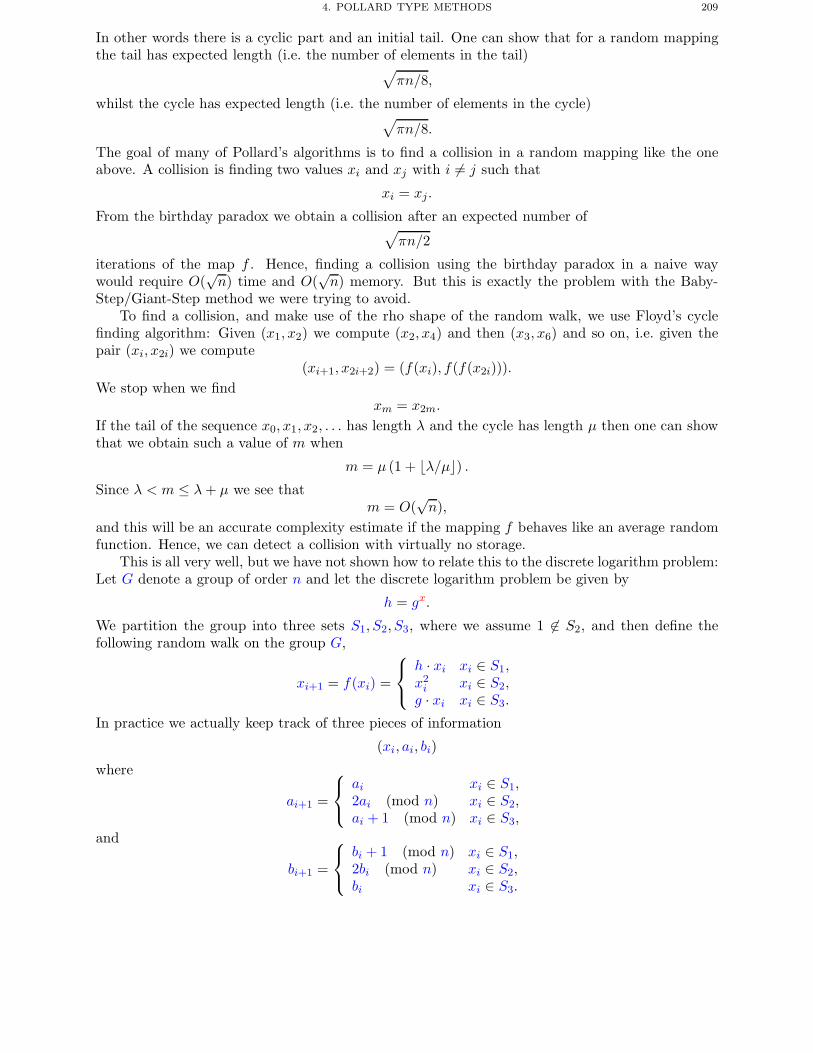
4. POLLARD TYPE METHODS 209
In other words there is a cyclic part and an initial tail. One can show that for a random mappingthe tail has expected length (i.e. the number of elements in the tail)√
πn/8,
whilst the cycle has expected length (i.e. the number of elements in the cycle)√πn/8.
The goal of many of Pollard’s algorithms is to find a collision in a random mapping like the oneabove. A collision is finding two values xi and xj with i �= j such that
xi = xj.
From the birthday paradox we obtain a collision after an expected number of√πn/2
iterations of the map f . Hence, finding a collision using the birthday paradox in a naive waywould require O(
√n) time and O(
√n) memory. But this is exactly the problem with the Baby-
Step/Giant-Step method we were trying to avoid.To find a collision, and make use of the rho shape of the random walk, we use Floyd’s cycle
finding algorithm: Given (x1, x2) we compute (x2, x4) and then (x3, x6) and so on, i.e. given thepair (xi, x2i) we compute
(xi+1, x2i+2) = (f(xi), f(f(x2i))).We stop when we find
xm = x2m.
If the tail of the sequence x0, x1, x2, . . . has length λ and the cycle has length μ then one can showthat we obtain such a value of m when
m = μ (1 + �λ/μ�) .Since λ < m ≤ λ+ μ we see that
m = O(√n),
and this will be an accurate complexity estimate if the mapping f behaves like an average randomfunction. Hence, we can detect a collision with virtually no storage.
This is all very well, but we have not shown how to relate this to the discrete logarithm problem:Let G denote a group of order n and let the discrete logarithm problem be given by
h = gx.
We partition the group into three sets S1, S2, S3, where we assume 1 �∈ S2, and then define thefollowing random walk on the group G,
xi+1 = f(xi) =
⎧⎨⎩
h · xi xi ∈ S1,x2i xi ∈ S2,g · xi xi ∈ S3.
In practice we actually keep track of three pieces of information
(xi, ai, bi)
where
ai+1 =
⎧⎨⎩
ai xi ∈ S1,2ai (mod n) xi ∈ S2,ai + 1 (mod n) xi ∈ S3,
and
bi+1 =
⎧⎨⎩
bi + 1 (mod n) xi ∈ S1,2bi (mod n) xi ∈ S2,bi xi ∈ S3.
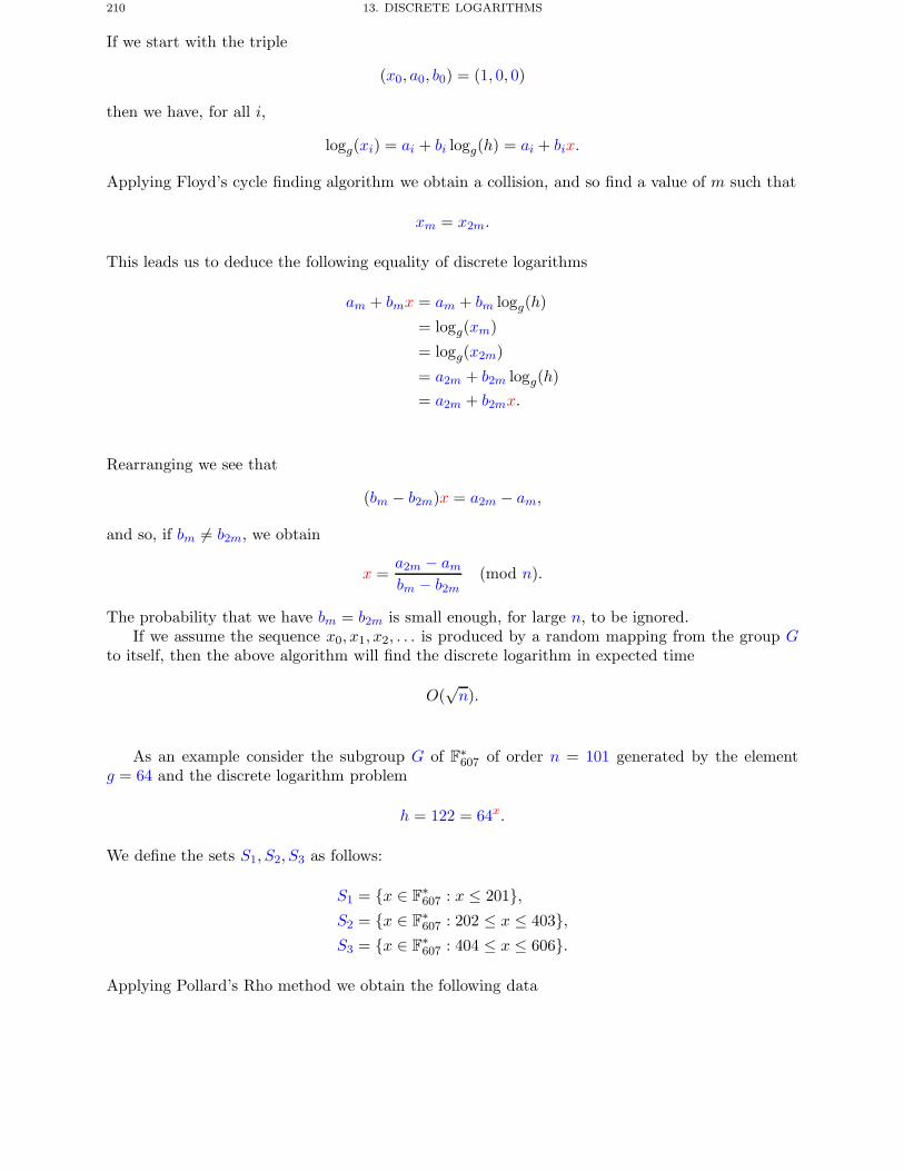
210 13. DISCRETE LOGARITHMS
If we start with the triple
(x0, a0, b0) = (1, 0, 0)
then we have, for all i,
logg(xi) = ai + bi logg(h) = ai + bix.
Applying Floyd’s cycle finding algorithm we obtain a collision, and so find a value of m such that
xm = x2m.
This leads us to deduce the following equality of discrete logarithms
am + bmx = am + bm logg(h)
= logg(xm)
= logg(x2m)
= a2m + b2m logg(h)= a2m + b2mx.
Rearranging we see that
(bm − b2m)x = a2m − am,
and so, if bm �= b2m, we obtain
x =a2m − ambm − b2m
(mod n).
The probability that we have bm = b2m is small enough, for large n, to be ignored.If we assume the sequence x0, x1, x2, . . . is produced by a random mapping from the group G
to itself, then the above algorithm will find the discrete logarithm in expected time
O(√n).
As an example consider the subgroup G of F∗607 of order n = 101 generated by the element
g = 64 and the discrete logarithm problem
h = 122 = 64x.
We define the sets S1, S2, S3 as follows:
S1 = {x ∈ F∗607 : x ≤ 201},
S2 = {x ∈ F∗607 : 202 ≤ x ≤ 403},
S3 = {x ∈ F∗607 : 404 ≤ x ≤ 606}.
Applying Pollard’s Rho method we obtain the following data
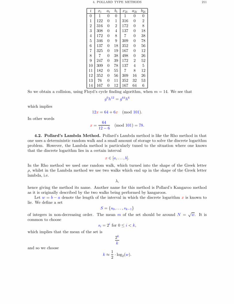
4. POLLARD TYPE METHODS 211
i xi ai bi x2i a2i b2i0 1 0 0 1 0 01 122 0 1 316 0 22 316 0 2 172 0 83 308 0 4 137 0 184 172 0 8 7 0 385 346 0 9 309 0 786 137 0 18 352 0 567 325 0 19 167 0 128 7 0 38 498 0 269 247 0 39 172 2 5210 309 0 78 137 4 511 182 0 55 7 8 1212 352 0 56 309 16 2613 76 0 11 352 32 5314 167 0 12 167 64 6
So we obtain a collision, using Floyd’s cycle finding algorithm, when m = 14. We see that
g0h12 = g64h6
which implies12x = 64 + 6x (mod 101).
In other words
x =64
12 − 6(mod 101) = 78.
4.2. Pollard’s Lambda Method. Pollard’s Lambda method is like the Rho method in thatone uses a deterministic random walk and a small amount of storage to solve the discrete logarithmproblem. However, the Lambda method is particularly tuned to the situation where one knowsthat the discrete logarithm lies in a certain interval
x ∈ [a, . . . , b].
In the Rho method we used one random walk, which turned into the shape of the Greek letterρ, whilst in the Lambda method we use two walks which end up in the shape of the Greek letterlambda, i.e.
λ,
hence giving the method its name. Another name for this method is Pollard’s Kangaroo methodas it is originally described by the two walks being performed by kangaroos.
Let w = b− a denote the length of the interval in which the discrete logarithm x is known tolie. We define a set
S = {s0, . . . , sk−1}of integers in non-decreasing order. The mean m of the set should be around N =
√w. It is
common to choosesi = 2i for 0 ≤ i < k,
which implies that the mean of the set is2k
kand so we choose
k ≈ 12· log2(w).
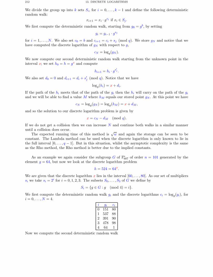
212 13. DISCRETE LOGARITHMS
We divide the group up into k sets Si, for i = 0, . . . , k − 1 and define the following deterministicrandom walk:
xi+1 = xi · gsj if xi ∈ Sj .
We first compute the deterministic random walk, starting from g0 = gb, by setting
gi = gi−1 · gsjfor i = 1, . . . ,N . We also set c0 = b and ci+1 = ci + sj (mod q). We store gN and notice that wehave computed the discrete logarithm of gN with respect to g,
cN = logg(gN ).
We now compute our second deterministic random walk starting from the unknown point in theinterval x; we set h0 = h = gx and compute
hi+1 = hi · gs′j .
We also set d0 = 0 and di+1 = di + s′j (mod q). Notice that we have
logg(hi) = x+ di.
If the path of the hi meets that of the path of the gi then the hi will carry on the path of the giand we will be able to find a value M where hM equals our stored point gN . At this point we have
cN = logg(gN ) = logg(hM ) = x+ dM ,
and so the solution to our discrete logarithm problem is given by
x = cN − dM (mod q).
If we do not get a collision then we can increase N and continue both walks in a similar manneruntil a collision does occur.
The expected running time of this method is√w and again the storage can be seen to be
constant. The Lambda method can be used when the discrete logarithm is only known to lie inthe full interval [0, . . . , q − 1]. But in this situation, whilst the asymptotic complexity is the sameas the Rho method, the Rho method is better due to the implied constants.
As an example we again consider the subgroup G of F∗607 of order n = 101 generated by the
element g = 64, but now we look at the discrete logarithm problem
h = 524 = 64x.
We are given that the discrete logarithm x lies in the interval [60, . . . , 80]. As our set of multiplierssi we take si = 2i for i = 0, 1, 2, 3. The subsets S0, . . . , S3 of G we define by
Si = {g ∈ G : g (mod 4) = i}.We first compute the deterministic random walk gi and the discrete logarithms ci = logg(gi), fori = 0, . . . ,N = 4.
i gi ci0 151 801 537 882 391 903 478 984 64 1
Now we compute the second deterministic random walk
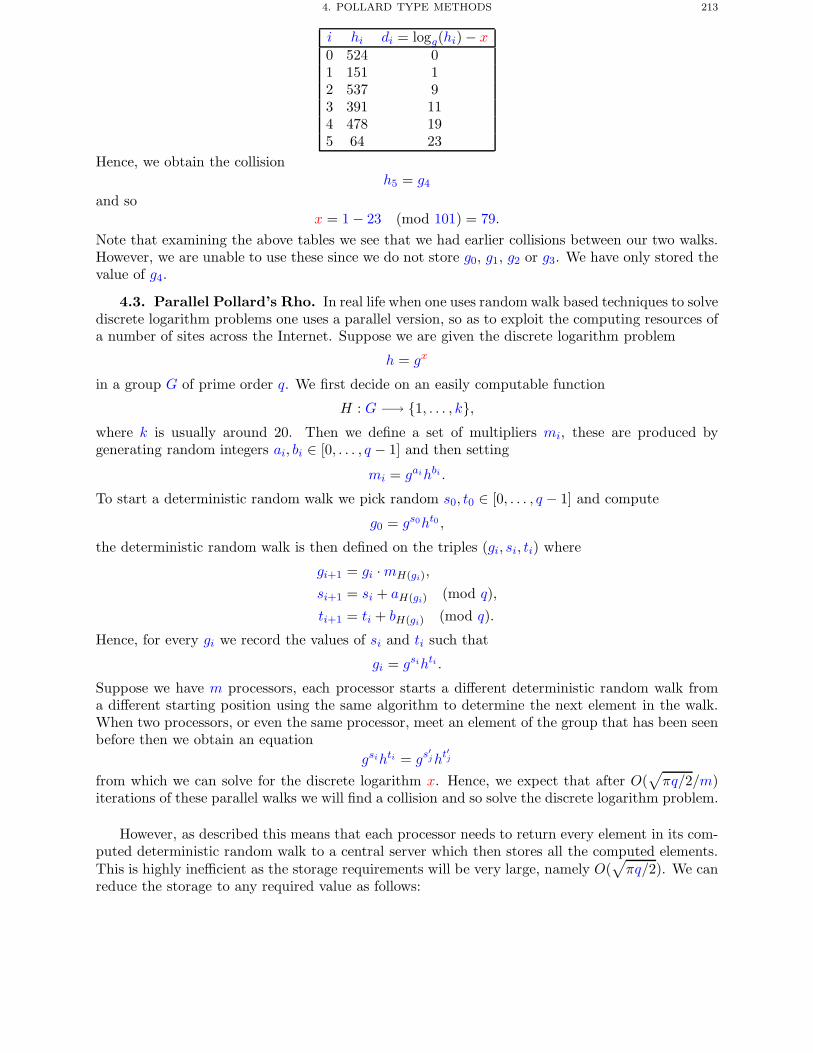
4. POLLARD TYPE METHODS 213
i hi di = logg(hi) − x0 524 01 151 12 537 93 391 114 478 195 64 23
Hence, we obtain the collisionh5 = g4
and sox = 1 − 23 (mod 101) = 79.
Note that examining the above tables we see that we had earlier collisions between our two walks.However, we are unable to use these since we do not store g0, g1, g2 or g3. We have only stored thevalue of g4.
4.3. Parallel Pollard’s Rho. In real life when one uses random walk based techniques to solvediscrete logarithm problems one uses a parallel version, so as to exploit the computing resources ofa number of sites across the Internet. Suppose we are given the discrete logarithm problem
h = gx
in a group G of prime order q. We first decide on an easily computable function
H : G −→ {1, . . . , k},where k is usually around 20. Then we define a set of multipliers mi, these are produced bygenerating random integers ai, bi ∈ [0, . . . , q − 1] and then setting
mi = gaihbi .
To start a deterministic random walk we pick random s0, t0 ∈ [0, . . . , q − 1] and compute
g0 = gs0ht0 ,
the deterministic random walk is then defined on the triples (gi, si, ti) where
gi+1 = gi ·mH(gi),
si+1 = si + aH(gi) (mod q),
ti+1 = ti + bH(gi) (mod q).
Hence, for every gi we record the values of si and ti such that
gi = gsihti .
Suppose we have m processors, each processor starts a different deterministic random walk froma different starting position using the same algorithm to determine the next element in the walk.When two processors, or even the same processor, meet an element of the group that has been seenbefore then we obtain an equation
gsihti = gs′jht
′j
from which we can solve for the discrete logarithm x. Hence, we expect that after O(√πq/2/m)
iterations of these parallel walks we will find a collision and so solve the discrete logarithm problem.
However, as described this means that each processor needs to return every element in its com-puted deterministic random walk to a central server which then stores all the computed elements.This is highly inefficient as the storage requirements will be very large, namely O(
√πq/2). We can
reduce the storage to any required value as follows:
214 13. DISCRETE LOGARITHMS
We define a function d on the group
d : G −→ {0, 1}such that d(g) = 1 around 1/2t of the time. The function d is often defined by returning d(g) = 1if a certain subset of t of the bits representing g are set to zero for example. The elements in G forwhich d(g) = 1 will be called distinguished.
It is only the distinguished group elements which are now transmitted back to the central server.This means that one expects the deterministic random walks to need to continue another 2t stepsbefore a collision is detected between two deterministic random walks. Hence, the computing timenow becomes
O(√
πq/2/m+ 2t),
whilst the storage becomes
O(√
πq/2/2t).
This allows the storage to be reduced to any manageable amount, at the expense of a little extracomputation. We do not give an example, since the method only really becomes useful as q becomeslarger (say q > 220), but we leave it to the reader to construct their own examples.
5. Sub-exponential Methods for Finite Fields
There is a close relationship between the sub-exponential methods for factoring and the sub-exponential methods for solving the discrete logarithm problem in finite fields. We shall onlyconsider the case of prime fields Fp but similar considerations apply to finite fields of character-istic two. The sub-exponential algorithms for finite fields are often referred to as index-calculusalgorithms, for a reason which will become apparent as we explain the method.
We assume we are given g, h ∈ F∗p such that
h = gx.
We choose a factor base F of elements, usually small prime numbers, and then using one of thesieving strategies used for factoring we obtain a large number of relations of the form∏
pi∈Fpeii = 1 (mod p).
These relations translate into the following equations for discrete logarithms,∑pi∈F
ei logg(pi) = 0 (mod p− 1).
Once enough equations like the one above have been found we can solve for the discrete logarithmof every element in the factor base, i.e. we can determine
xi = logg(pi).
The value of xi is sometimes called the index of pi with respect to g. This calculation is performedusing linear algebra modulo p−1, which is hence more complicated than the linear algebra modulo2 performed in factoring algorithms. However, similar tricks, such as those deployed in the linearalgebra stage of factoring algorithms, can be deployed to keep the storage requirements down tomanageable levels. This linear algebra calculation only needs to be done once for each generator g,the results can then be used for many values of h.
When one wishes to solve a particular discrete logarithm problem
h = gx,
6. SPECIAL METHODS FOR ELLIPTIC CURVES 215
we use a sieving technique, or simple trial and error, to write
h =∏pi∈F
phii (mod p),
i.e. we could computeT = h
∏pi∈F
pfii (mod p)
and see if it factors in the formT =
∏pi∈F
pgii .
If it does then we haveh =∏pi∈F
pigi−fi (mod p).
We can then compute the discrete logarithm x from
x = logg(h) = logg
⎛⎝∏pi∈F
phii
⎞⎠
=∑pi∈F
hi logg(pi) (mod p− 1)
=∑pi∈F
hi · xi (mod p− 1).
This means that, once one discrete logarithm has been found, determining the next one is easiersince we have already computed the values of the xi.
The best of the methods to find the relations between the factorbase elements is the NumberField Sieve. This gives an overall running time of
O(Lp(1/3, c))
for some constant c. This is roughly the same complexity as the algorithms to factor large numbers,although the real practical problem is that the matrix algorithms now need to work modulo p− 1and not modulo 2 as they did in factoring algorithms.
The upshot of these sub-exponential methods is that the size of p for finite field discrete loga-rithm based systems needs to be of the same order of magnitude as an RSA modulus, i.e. p ≥ 21024.
Even though p has to be very large we still need to guard against generic attacks, hence p− 1should have a prime factor q of order greater than 2160. In fact for finite field based systems weusually work in the subgroup of F∗
p of order q.
6. Special Methods for Elliptic Curves
For elliptic curves there are no known sub-exponential methods for the discrete logarithmproblem, except in certain special cases. This means that the only method to solve the discretelogarithm problem in this setting is the parallel version of Pollard’s Rho method.
Suppose the elliptic curve E is defined over the finite field Fq. We set
#E(Fq) = h · rwhere r is a prime number. By Hasse’s Theorem 2.3 the value of #E(Fq) is close to q so we typicallychoose a curve with r close to q, i.e. we choose a curve E so that h = 1, 2 or 4.
The best known general algorithm for the elliptic curve discrete logarithm problem is the parallelPollard’s Rho method, which has complexity O(
√r), which is about O(
√q). Hence, to achieve the
same security as an 80-bit block cipher we need to take q ≈ 2160, which is a lot smaller than the
216 13. DISCRETE LOGARITHMS
field size recommended for systems based on the discrete logarithm problems in a finite field. Thisresults in the reduced bandwidth and computational times of elliptic curve systems.
However, there are a number of special cases which need to be avoided. We shall now givethese special cases, but we shall not give the detailed reasons why they are to be avoided since thereasons are often quite mathematically involved. As usual we assume q is either a large prime or apower of 2.
• For any q we must choose curves for which there is no small number t such that r dividesqt − 1, where r is the large prime factor of #E(Fq). This eliminates the supersingularcurves and a few others. In this case there is a simple computable mapping from theelliptic curve discrete logarithm problem to the discrete logarithm problem in the finitefield Fqt . Hence, in this case we obtain a sub-exponential method for solving the ellipticcurve discrete logarithm problem.
• If q = p is a large prime then we need to avoid the anomalous curves where E(Fp) = p. Inthis case there is an algorithm which requires O(log p) elliptic curve operations.
• If q = 2n then we usually assume that n is prime to avoid the possibility of certain attacksbased on the concept of ‘Weil descent’.
One should treat these three special cases much like one treats the generation of large integers forthe RSA algorithm. Due to the P − 1 factoring method one often makes RSA moduli N = p · qsuch that p is a so-called safe prime of the form 2p1 +1. Another special RSA based case is that wealmost always use RSA with two prime factors, rather than three or four. This is because moduliwith two prime factors appear to be the hardest to factor.
Chapter Summary
• Due to the Pohlig–Hellman algorithm a hard discrete logarithm problem should be set ina group whose order has a large prime factor.
• The generic algorithms such as the Baby-Step/Giant-Step algorithm mean that to achievethe same security as an 80-bit block cipher, the size of this large prime factor of the grouporder should be at least 160 bits.
• The Baby-Step/Giant-Step algorithm is a generic algorithm whose running time can beabsolutely bounded by
√q, where q is the size of the large prime factor of #G. However,
the storage requirements of the Baby-Step/Giant-Step algorithm are O(√q).
• There are a number of techniques, due to Pollard, based on deterministic random walksin a group. These are generic algorithms which require little storage but which solve thediscrete logarithm problem in expected time O(
√q).
• For finite fields a number of index calculus algorithms exist which run in sub-exponentialtime. These mean that one needs to take large finite fields Fpt with pt ≥ 21024 if one wantsto obtain a hard discrete logarithm problem.
• For elliptic curves there are no sub-exponential algorithms known, except in very specialcases. Hence, the only practical general algorithm to solve the discrete logarithm problemon an elliptic curve is the parallel Pollard’s Rho method.
Further Reading
Further Reading 217
There are a number of good surveys on the discrete logarithm problem. I would recommend theones by McCurley and Odlyzko. These articles only touch on the elliptic curve discrete logarithmproblem though. For a treatment of what is known on the latter problem you could consult thesurvey by Koblitz et al.
N. Koblitz, A. Menezes and S. Vanstone. The state of elliptic curve cryptography. Designs Codesand Cryptography, 19, 173–193, 2000.
K. McCurley. The discrete logarithm problem. In Cryptology and Computational Number Theory,Proc. Symposia in Applied Maths, Volume 42, 1990.
A. Odlyzko. Discrete logarithms: The past and the future. Designs Codes and Cryptography, 19,129–145, 2000.

CHAPTER 14
Key Exchange and Signature Schemes
Chapter Goals
• To introduce Diffie–Hellman key exchange.• To introduce the need for digital signatures.• To explain the two most used signature algorithms, namely RSA and DSA.• To explain the need for cryptographic hash functions within signature schemes.• To describe some other signature algorithms and key exchange techniques which have
interesting properties.
1. Diffie–Hellman Key Exchange
Recall that the main drawback with the use of fast bulk encryption based on block or streamciphers was the problem of key distribution. We have already seen a number of techniques to solvethis problem, either using protocols which are themselves based on symmetric key techniques, orusing a public key algorithm to transport a session key to the intended recipient. These, however,both have problems associated with them. For example, the symmetric key protocols were hard toanalyse and required the use of already deployed long-term keys between each user and a trustedcentral authority.
A system is said to have forward secrecy, if the compromise of a long-term private key at somepoint in the future does not compromise the security of communications made using that key inthe past. Key transport via public key encryption does not have forward secrecy. To see why thisis important, suppose you bulk encrypt a video stream and then encrypt the session key under therecipient’s RSA public key. Then suppose that some time in the future, the recipient’s RSA privatekey is compromised. At that point your video stream is also compromised, assuming the attackerrecorded this at the time it was transmitted.
In addition using key transport implies that the recipient trusts the sender to be able to generate,in a sensible way, the session key. Sometimes the recipient may wish to contribute some randomnessof their own to the session key. However, this can only be done if both parties are online at thesame moment in time. Key transport is more suited to the case where only the sender is online, asin applications like email for example.
The key distribution problem was solved in the same seminal paper by Diffie and Hellman asthat in which they introduced public key cryptography. Their protocol for key distribution, calledDiffie–Hellman Key Exchange, allows two parties to agree a secret key over an insecure channelwithout having met before. Its security is based on the discrete logarithm problem in a finiteabelian group G.
219
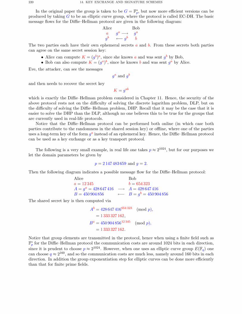
220 14. KEY EXCHANGE AND SIGNATURE SCHEMES
In the original paper the group is taken to be G = F∗p, but now more efficient versions can be
produced by taking G to be an elliptic curve group, where the protocol is called EC-DH. The basicmessage flows for the Diffie–Hellman protocol are given in the following diagram:
Alice Boba ga −→ ga
gb ←− gb b
The two parties each have their own ephemeral secrets a and b. From these secrets both partiescan agree on the same secret session key:
• Alice can compute K = (gb)a, since she knows a and was sent gb by Bob,• Bob can also compute K = (ga)b, since he knows b and was sent ga by Alice.
Eve, the attacker, can see the messages
ga and gb
and then needs to recover the secret key
K = gab
which is exactly the Diffie–Hellman problem considered in Chapter 11. Hence, the security of theabove protocol rests not on the difficulty of solving the discrete logarithm problem, DLP, but onthe difficulty of solving the Diffie–Hellman problem, DHP. Recall that it may be the case that it iseasier to solve the DHP than the DLP, although no one believes this to be true for the groups thatare currently used in real-life protocols.
Notice that the Diffie–Hellman protocol can be performed both online (in which case bothparties contribute to the randomness in the shared session key) or offline, where one of the partiesuses a long-term key of the form ga instead of an ephemeral key. Hence, the Diffie–Hellman protocolcan be used as a key exchange or as a key transport protocol.
The following is a very small example, in real life one takes p ≈ 21024, but for our purposes welet the domain parameters be given by
p = 2147 483 659 and g = 2.
Then the following diagram indicates a possible message flow for the Diffie–Hellman protocol:Alice Boba = 12345 b = 654 323A = ga = 428 647 416 −→ A = 428 647 416B = 450 904 856 ←− B = gb = 450 904 856
The shared secret key is then computed via
Ab = 428 647 416654 323 (mod p),= 1333 327 162,
Ba = 450 904 85612 345 (mod p),= 1333 327 162.
Notice that group elements are transmitted in the protocol, hence when using a finite field such asF∗p for the Diffie–Hellman protocol the communication costs are around 1024 bits in each direction,
since it is prudent to choose p ≈ 21024. However, when one uses an elliptic curve group E(Fq) onecan choose q ≈ 2160, and so the communication costs are much less, namely around 160 bits in eachdirection. In addition the group exponentiation step for elliptic curves can be done more efficientlythan that for finite prime fields.
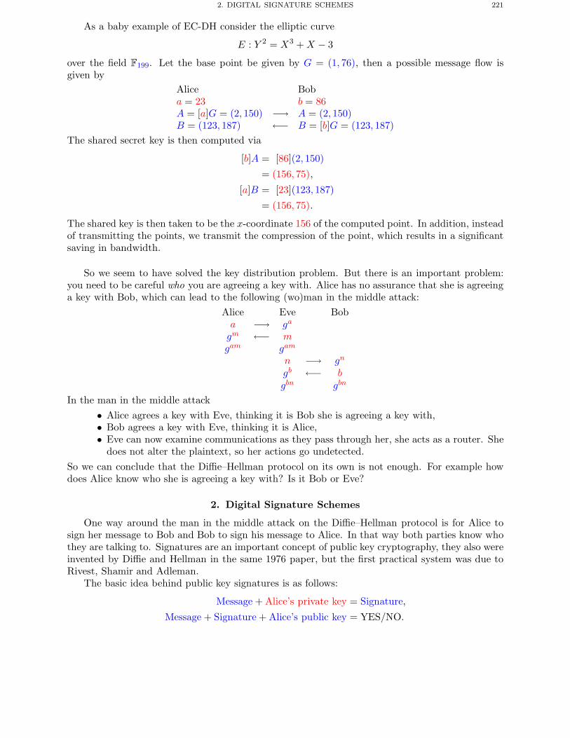
2. DIGITAL SIGNATURE SCHEMES 221
As a baby example of EC-DH consider the elliptic curve
E : Y 2 = X3 +X − 3
over the field F199. Let the base point be given by G = (1, 76), then a possible message flow isgiven by
Alice Boba = 23 b = 86A = [a]G = (2, 150) −→ A = (2, 150)B = (123, 187) ←− B = [b]G = (123, 187)
The shared secret key is then computed via
[b]A = [86](2, 150)
= (156, 75),
[a]B = [23](123, 187)
= (156, 75).
The shared key is then taken to be the x-coordinate 156 of the computed point. In addition, insteadof transmitting the points, we transmit the compression of the point, which results in a significantsaving in bandwidth.
So we seem to have solved the key distribution problem. But there is an important problem:you need to be careful who you are agreeing a key with. Alice has no assurance that she is agreeinga key with Bob, which can lead to the following (wo)man in the middle attack:
Alice Eve Boba −→ ga
gm ←− mgam gam
n −→ gn
gb ←− bgbn gbn
In the man in the middle attack• Alice agrees a key with Eve, thinking it is Bob she is agreeing a key with,• Bob agrees a key with Eve, thinking it is Alice,• Eve can now examine communications as they pass through her, she acts as a router. She
does not alter the plaintext, so her actions go undetected.So we can conclude that the Diffie–Hellman protocol on its own is not enough. For example howdoes Alice know who she is agreeing a key with? Is it Bob or Eve?
2. Digital Signature Schemes
One way around the man in the middle attack on the Diffie–Hellman protocol is for Alice tosign her message to Bob and Bob to sign his message to Alice. In that way both parties know whothey are talking to. Signatures are an important concept of public key cryptography, they also wereinvented by Diffie and Hellman in the same 1976 paper, but the first practical system was due toRivest, Shamir and Adleman.
The basic idea behind public key signatures is as follows:
Message + Alice’s private key = Signature,
Message + Signature + Alice’s public key = YES/NO.
222 14. KEY EXCHANGE AND SIGNATURE SCHEMES
The above is called a signature scheme with appendix, since the signature is appended to themessage before transmission, the message needs to be input into the signature verification procedure.Another variant is the signature scheme with message recovery, where the message is output bythe signature verification procedure, as described in
Message + Alice’s private key = Signature,
Signature + Alice’s public key = YES/NO + Message.
The main idea is that only Alice can sign a message, which could only come from her since onlyAlice has access to the private key. On the other hand anyone can verify Alice’s signature, sinceeveryone can have access to her public key.
The main problem is how are the public keys to be trusted? How do you know a certain publickey is associated to a given entity? You may think a public key belongs to Alice, but it may belongto Eve. Eve can therefore sign cheques etc., and you would think they come from Alice. We seemto have the same key management problem as in symmetric systems, albeit now the problem is notone of keeping the keys secret, but making sure they are authentic. We shall return to this problemlater.
A digital signature scheme consists more formally of two transformations:• a secret signing transform S,• a public verification transform V.
In the following discussion, we assume a signature with message recovery. For an appendix basedscheme a simple change to the following will suffice.
Alice, sending a message m, calculates
s = S(m)
and then transmits s, where s is the digital signature on the message m. Note, we are not interestedin keeping the message secret here, since we are only interested in knowing who it comes from. Ifconfidentiality of the message is important then the signature s could be encrypted using, forexample, the public key of the receiver.
The receiver of the signature s applies the public verification transform V to s. The output isthen the message m and a bit v. The bit v indicates valid or invalid, i.e. whether the signature isgood or not. If v is valid the recipient gets a guarantee of three important security properties:
• message integrity – the message has not been altered in transit,• message origin – the message was sent by Alice,• non-repudiation – Alice cannot claim she did not send the message.
Note, the first two of these properties are also provided by message authentication codes, MACs.However, the last property of non-repudiation is not provided by MACs and has important appli-cations in e-commerce. To see why non-repudiation is so important, consider what would happenif you could sign a cheque and then say you did not sign it.
The RSA encryption algorithm is particularly interesting since it can be used directly as asignature algorithm with message recovery.
• The sender applies the RSA decryption transform to generate the signature, by taking themessage and raising it to the private exponent d
s = md (mod N).
• The receiver then applies the RSA encryption transform to recover the original message
m = se (mod N).
3. THE USE OF HASH FUNCTIONS IN SIGNATURE SCHEMES 223
But this raises the question as to how do we check for validity of the signature? If the originalmessage is in a natural language such as English then one can verify that the extracted message isalso in the same natural language. But this is not a solution for all possible messages. Hence oneneeds to add redundancy to the message.
One way of doing this is as follows. Suppose the message D is t bits long and the RSA modulusN is k bits long, with t < k− 32. We first pad D to the right by zeros to produce a string of lengtha multiple of eight. We then add (k − t)/8 bytes to the left of D to produce a byte-string
m = 00‖01‖FF‖FF . . . ‖FF‖00‖D.The signature is then computed via
md (mod N).When verifying the signature we ensure that the recovered value of m has the correct padding.
But not all messages will be so short so as to fit into the above method. Hence, naively toapply the RSA signature algorithm to a long message m we need to break it into blocks and signeach block in turn. This is very time consuming for long messages. Worse than this, we must addserial numbers and more redundancy to each message otherwise an attacker could delete parts ofthe long message without us knowing, just as happened when encrypting using a block cipher inECB Mode. This problem arises because our signature model is one giving message recovery, i.e.the message is recovered from the signature and the verification process. If we used a system usinga signature scheme with appendix then we could produce a hash of the message to be signed andthen just sign the hash.
3. The Use of Hash Functions In Signature Schemes
Using a cryptographic hash function h, such as those described in Chapter 10, it is possible tomake RSA into a signature scheme without message recovery, which is much more efficient for longmessages.
Suppose we are given a long message m for signing, we first compute h(m) and then apply theRSA signing transform to h(m), i.e. the signature is given by
s = h(m)d (mod N).
The signature and message are then transmitted together as the pair (m, s). Verifying a mes-sage/signature pair (m, s) generated using a hash function involves three steps.
• ‘Encrypt’ s using the RSA encryption function to recover h′, i.e.
h′ = se (mod N).
• Compute h(m) from m.• Check whether h′ = h(m). If they agree accept the signature as valid, otherwise the
signature should be rejected.Actually in practice one also needs padding, as a hash function usually does not have output thewhole of the integers modulo N . You could use the padding scheme given earlier when we discussedRSA with message recovery.
Recall that a cryptographic hash function needs to satisfy the following three properties:(1) Preimage Resistant: It should be hard to find a message with a given hash value.(2) Collision Resistant: It should be hard to find two messages with the same hash value.(3) Second Preimage Resistant: Given one message it should be hard to find another
message with the same hash value.So why do we need to use a hash function which has these properties within the above signaturescheme? We shall address these issues below:
224 14. KEY EXCHANGE AND SIGNATURE SCHEMES
3.1. Requirement for preimage resistance. The one-way property stops a cryptanalystfrom cooking up a message with a given signature. For example, suppose we are using the RSAscheme with appendix just described but with a hash function which does not have the one-wayproperty. We then have the following attack.
• Eve computesh′ = re (mod N)
for some random integer r.• Eve also computes the pre-image of h′ under h (recall we are assuming that h does not
have the one-way property) i.e. Eve computes
m = h−1(h′).
Eve now has your signature (m, r) on the message m. Such a forgery is called an existential forgeryin that the attacker may not have any control over the contents of the message on which they haveobtained a digital signature.
3.2. Requirement for collision resistance. This is needed to avoid the following attack,which is performed by the legitimate signer.
• The signer chooses two messages m and m′ with h(m) = h(m′).• They sign m and output the signature (m, s).• Later they repudiate this signature, saying it was really a signature on the message m′.
As a concrete example one could have that m is an electronic cheque for 1000 euros whilst m′ is anelectronic cheque for 10 euros.
3.3. Requirement for second preimage resistance. This property is needed to stop thefollowing attack.
• An attacker obtains your signature (m, s) on a message m.• The attacker finds another message m′ with h(m′) = h(m).• The attacker now has your signature (m′, s) on the message m′.
Note, the security of any signature scheme which uses a cryptographic hash function, dependsboth on the security of the underlying hard mathematical problem, such as factoring or the discretelogarithm problem, and the security of the underlying hash function.
4. The Digital Signature Algorithm
We have already presented one digital signature scheme RSA. You may ask why do we needanother one?
• What if someone breaks the RSA algorithm or finds that factoring is easy?• RSA is not suited to some applications since signature generation is a very costly operation.• RSA signatures are very large, some applications require smaller signature footprints.
One algorithm which addresses all of these concerns is the Digital Signature Algorithm, or DSA.One sometimes sees this referred to as the DSS, or Digital Signature Standard. Although originallydesigned to work in the group F∗
p, where p is a large prime, it is now common to see it used usingelliptic curves, in which case it is called EC-DSA. The elliptic curve variants of DSA run very fastand have smaller footprints and key sizes than almost all other signature algorithms.
We shall first describe the basic DSA algorithm as it applies to finite fields. In this variant thesecurity is based on the difficulty of solving the discrete logarithm problem in the field Fp.
DSA is a signature with appendix algorithm and the signature produced consists of two 160-bitintegers r and s. The integer r is a function of a 160-bit random number k called the ephemeralkey which changes with every message. The integer s is a function of
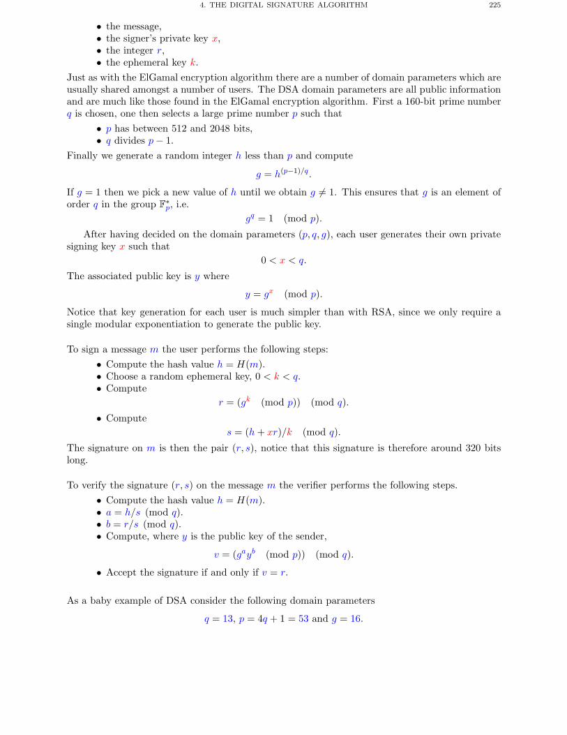
4. THE DIGITAL SIGNATURE ALGORITHM 225
• the message,• the signer’s private key x,• the integer r,• the ephemeral key k.
Just as with the ElGamal encryption algorithm there are a number of domain parameters which areusually shared amongst a number of users. The DSA domain parameters are all public informationand are much like those found in the ElGamal encryption algorithm. First a 160-bit prime numberq is chosen, one then selects a large prime number p such that
• p has between 512 and 2048 bits,• q divides p− 1.
Finally we generate a random integer h less than p and compute
g = h(p−1)/q.
If g = 1 then we pick a new value of h until we obtain g �= 1. This ensures that g is an element oforder q in the group F∗
p, i.e.gq = 1 (mod p).
After having decided on the domain parameters (p, q, g), each user generates their own privatesigning key x such that
0 < x < q.
The associated public key is y where
y = gx (mod p).
Notice that key generation for each user is much simpler than with RSA, since we only require asingle modular exponentiation to generate the public key.
To sign a message m the user performs the following steps:• Compute the hash value h = H(m).• Choose a random ephemeral key, 0 < k < q.• Compute
r = (gk (mod p)) (mod q).
• Computes = (h+ xr)/k (mod q).
The signature on m is then the pair (r, s), notice that this signature is therefore around 320 bitslong.
To verify the signature (r, s) on the message m the verifier performs the following steps.• Compute the hash value h = H(m).• a = h/s (mod q).• b = r/s (mod q).• Compute, where y is the public key of the sender,
v = (gayb (mod p)) (mod q).
• Accept the signature if and only if v = r.
As a baby example of DSA consider the following domain parameters
q = 13, p = 4q + 1 = 53 and g = 16.
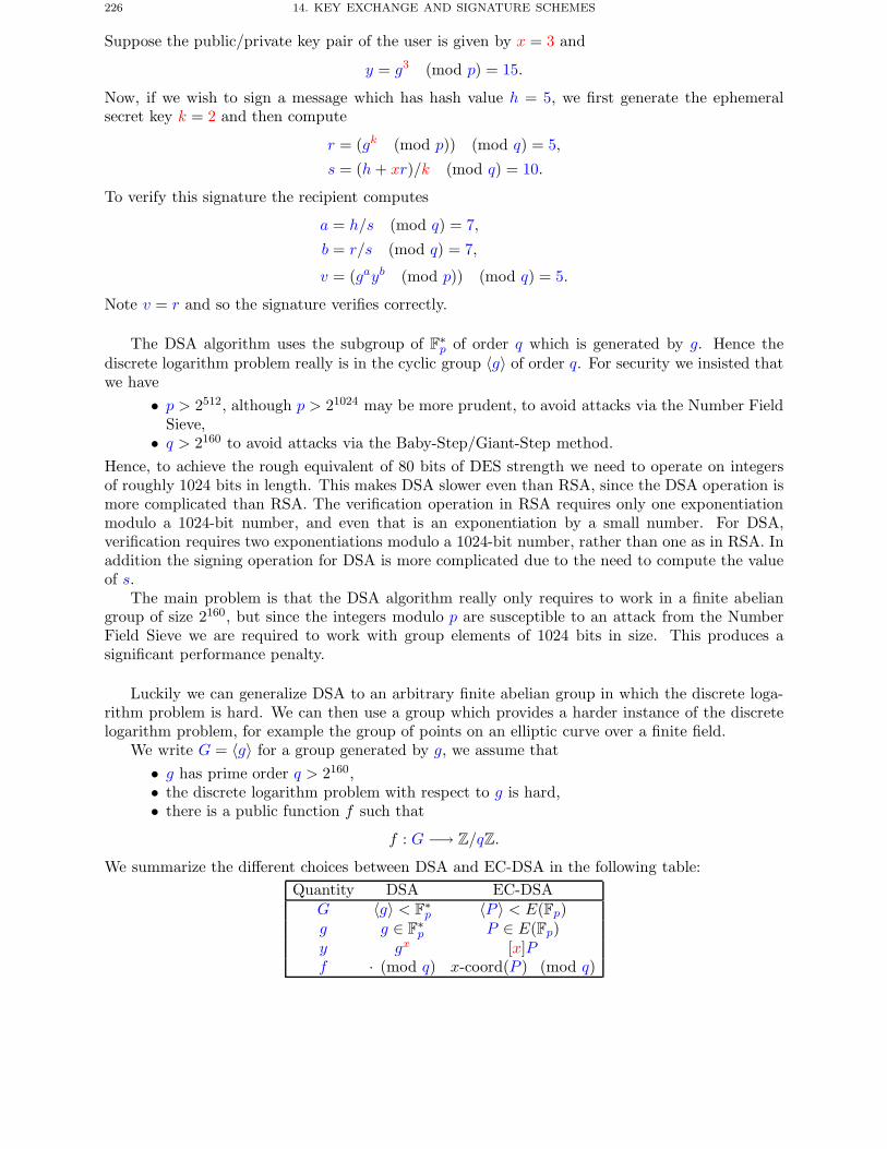
226 14. KEY EXCHANGE AND SIGNATURE SCHEMES
Suppose the public/private key pair of the user is given by x = 3 and
y = g3 (mod p) = 15.
Now, if we wish to sign a message which has hash value h = 5, we first generate the ephemeralsecret key k = 2 and then compute
r = (gk (mod p)) (mod q) = 5,
s = (h+ xr)/k (mod q) = 10.
To verify this signature the recipient computes
a = h/s (mod q) = 7,
b = r/s (mod q) = 7,
v = (gayb (mod p)) (mod q) = 5.
Note v = r and so the signature verifies correctly.
The DSA algorithm uses the subgroup of F∗p of order q which is generated by g. Hence the
discrete logarithm problem really is in the cyclic group 〈g〉 of order q. For security we insisted thatwe have
• p > 2512, although p > 21024 may be more prudent, to avoid attacks via the Number FieldSieve,
• q > 2160 to avoid attacks via the Baby-Step/Giant-Step method.Hence, to achieve the rough equivalent of 80 bits of DES strength we need to operate on integersof roughly 1024 bits in length. This makes DSA slower even than RSA, since the DSA operation ismore complicated than RSA. The verification operation in RSA requires only one exponentiationmodulo a 1024-bit number, and even that is an exponentiation by a small number. For DSA,verification requires two exponentiations modulo a 1024-bit number, rather than one as in RSA. Inaddition the signing operation for DSA is more complicated due to the need to compute the valueof s.
The main problem is that the DSA algorithm really only requires to work in a finite abeliangroup of size 2160, but since the integers modulo p are susceptible to an attack from the NumberField Sieve we are required to work with group elements of 1024 bits in size. This produces asignificant performance penalty.
Luckily we can generalize DSA to an arbitrary finite abelian group in which the discrete loga-rithm problem is hard. We can then use a group which provides a harder instance of the discretelogarithm problem, for example the group of points on an elliptic curve over a finite field.
We write G = 〈g〉 for a group generated by g, we assume that• g has prime order q > 2160,• the discrete logarithm problem with respect to g is hard,• there is a public function f such that
f : G −→ Z/qZ.
We summarize the different choices between DSA and EC-DSA in the following table:Quantity DSA EC-DSA
G 〈g〉 < F∗p 〈P 〉 < E(Fp)
g g ∈ F∗p P ∈ E(Fp)
y gx [x]Pf · (mod q) x-coord(P ) (mod q)
4. THE DIGITAL SIGNATURE ALGORITHM 227
For this generalized form of DSA each user again generates a secret signing key, x. The public keyis again give by y where
y = gx.
Signatures are computed via the steps
• Compute the hash value h = H(m).• Chooses a random ephemeral key, 0 < k < q.• Compute
r = f(gk).
• Computes = (h+ xr)/k (mod q).
The signature on m is then the pair (r, s).To verify the signature (r, s) on the message m the verifier performs the following steps.
• Compute the hash value h = H(m).• a = h/s (mod q).• b = r/s (mod q).• Compute, where y is the public key of the sender,
v = f(gayb).
• Accept the signature if and only if v = r.
You should compare this signature and verification algorithm with that given earlier for DSA andspot where they differ. When used for EC-DSA the above generalization is written additively.
As a baby example of EC-DSA take the following elliptic curve
Y 2 = X3 +X + 3,
over the field F199. The number of elements in E(F199) is equal to q = 197 which is a prime, theelliptic curve group is therefore cyclic and as a generator we can take
P = (1, 76).
As a private key let us take x = 29, and so the associated public key is given by
Y = [x]P = [29](1, 76) = (113, 191).
Suppose the holder of this public key wishes to sign a message with hash value H(m) equal to 68.They first produce a random ephemeral key, which we shall take to be k = 153 and compute
r = x-coord ([k]P )
= x-coord ([153](1, 76))
= x-coord ((185, 35))= 185.
Now they compute
s = (H(m) + x · r)/k (mod q)
= (68 + 29 · 185)/153 (mod 197)= 78.
The signature is then the pair (r, s) = (185, 78).
228 14. KEY EXCHANGE AND SIGNATURE SCHEMES
To verify this signature we compute
a = H(m)/s (mod q)
= 68/78 (mod 197)= 112,
b = r/s (mod q)
= 185/78 (mod 197)= 15.
We then compute
Z = [a]P + [b]Y
= [112](1, 76) + [15](113, 191)
= (111, 60) + (122, 140)
= (185, 35).
The signature now verifies since we have
r = 185 = x-coord(Z).
5. Schnorr Signatures
There are many variants of signature schemes based on discrete logarithms. A particularlyinteresting one is that of Schnorr signatures. We present the algorithm in the general case andallow the reader to work out the differences between the elliptic curve and finite field variants.
Suppose G is a public finite abelian group generated by an element g of prime order q. Thepublic/private key pairs are just the same as in DSA, namely
• The private key is an integer x in the range 0 < x < q.• The public key is the element
y = gx.
To sign a message m using the Schnorr signature algorithm we:(1) Choose an ephemeral key k in the range 0 < k < q.(2) Compute the associated ephemeral public key
r = gk.
(3) Compute e = h(m‖r). Notice how the hash function depends both on the message andthe ephemeral public key.
(4) Computes = k + x · e (mod q).
The signature is then given by the pair (e, s).The verification step is very simple, we first compute
r = gsy−e.
The signature is accepted if and only if e = h(m‖r).
As an example of Schnorr signatures in a finite field we take the domain parameters
q = 101, p = 607 and g = 601.
As the public/private key pair we assume x = 3 and
y = gx (mod p) = 391.
5. SCHNORR SIGNATURES 229
Then to sign a message we generate an ephemeral key k = 65 and compute
r = gk (mod p) = 223.
We now need to compute the hash value
e = h(m‖r) (mod q).
Let us assume that we compute e = 93, then the second component of the signature is given by
s = k + x · e (mod q)
= 65 + 3 · 93 (mod 101)= 41.
In a later chapter we shall see that Schnorr signatures are able to be proved to be secure,assuming that discrete logarithms are hard to compute, whereas no proof of security is known forDSA signatures.
Schnorr signatures have been suggested to be used for challenge response mechanisms in smartcards since the response part of the signature (the value of s) is particularly easy to evaluate sinceit only requires the computation of a single modular multiplication and a single modular addition.No matter what group we choose this final phase only requires arithmetic modulo a relatively smallprime number.
To see how one uses Schnorr signatures in a challenge response situation we give the followingscenario. A smart card wishes to authenticate you to a building or ATM machine. The card readerhas a copy of your public key y, whilst the card has a copy of your private key x. Whilst you arewalking around the card is generating commitments, which are ephemeral public keys of the form
r = gk.
When you place your card into the card reader the card transmits to the reader the value of oneof these precomputed commitments. The card reader then responds with a challenge message e.Your card then only needs to compute
s = k + xe (mod q),
and transmit it to the reader which then verifies the ‘signature’, by checking that
gs = rye.
Notice that the only online computation needed by the card is the computation of the value of eand s, which are both easy to perform.
In more detail, if we let C denote the card and R denote the card reader then we have
C −→ R : r = gk,
R −→ C : e,
C −→ R : s = k + xe (mod q).
The point of the initial commitment is to stop either the challenge being concocted so as to revealyour private key, or your response being concocted so as to fool the reader. A three-phase protocolconsisting of
commitment −→ challenge −→ response
is a common form of authentication protocols, we shall see more protocols of this nature when wediscuss zero-knowledge proofs in Chapter 25.
230 14. KEY EXCHANGE AND SIGNATURE SCHEMES
6. Nyberg–Rueppel Signatures
What happens when we want to sign a general message which is itself quite short. It may turnout that the signature could be longer than the message. Recall that RSA can be used either as ascheme with appendix or as a scheme with message recovery. So far none of our discrete logarithmbased schemes can be used with message recovery. We shall now give an example scheme whichdoes have the message recovery property, called the Nyberg–Rueppel signature scheme, which isbased on discrete logarithms in some public finite abelian group G.
All signature schemes with message recovery require a public redundancy function R. Thisfunction maps actual messages over to the data which is actually signed. This acts rather like ahash function does in the schemes based on signatures with appendix. However, unlike a hashfunction the redundancy function must be easy to invert. As a simple example we could take R tobe the function
R :
{{0, 1}n/2 −→ {0, 1}n
m −→ m‖m.We assume that the codomain of R can be embedded into the group G. In our description we shalluse the integers modulo p, i.e. G = F∗
p, and as usual we assume that a large prime q divides p − 1and that g is a generator of the subgroup of order q.
Once again the public/private key pair is given as a discrete logarithm problem
(y = gx, x).
Nyberg–Rueppel signatures are then produced as follows:(1) Select a random k ∈ Z/qZ and compute
r = gk (mod p).
(2) Computee = R(m) · r (mod p).
(3) Computes = x · e+ k (mod q).
The signature is then the pair (e, s). From this pair, which is a group element and an integermodulo q, we need to
• verify that the signature comes from the user with public key y,• recover the message m from the pair (e, s).
Verification for a Nyberg–Rueppel signature takes the signature (e, s) and the sender’s publickey y = gx and then computes
(1) Setu1 = gsy−e = gs−ex = gk (mod p).
(2) Now computeu2 = e/u1 (mod p).
(3) Verify that u2 lies in the range of the redundancy function, e.g. we must have
u2 = R(m) = m‖m.If this does not hold then reject the signature.
(4) Recover the message m = R−1(u2) and accept the signature.As an example we take the domain parameters
q = 101, p = 607 and g = 601.
As the public/private key pair we assume x = 3 and
y = gx (mod p) = 391.
7. AUTHENTICATED KEY AGREEMENT 231
To sign the message m = 12, where m must lie in [0, . . . , 15], we compute an ephemeral key k = 45and
r = gk (mod p) = 143.Suppose
R(m) = m+ 24 ·mthen we have R(m) = 204. We then compute
e = R(m) · r (mod p) = 36,
s = x · e+ k (mod q) = 52.
The signature is then the pair (e, s) = (36, 52). We now show how this signature is verified and themessage recovered. We first compute
u1 = gsy−e = 143.
Notice how the verifier has computed u1 to be the same as the value of r computed by the signer.The verifier now computes
u2 = e/u1 (mod p) = 204.The verifier now checks that u2 = 204 is of the form
m+ 24m
for some value of m ∈ [0, . . . , 15]. We see that u2 is of this form and so the signature is valid. Themessage is then recovered by solving for m in
m+ 24m = 204,
from which we obtain m = 12.
7. Authenticated Key Agreement
Now we know how to perform digital signatures we can solve the problem with Diffie–Hellmankey exchange. Recall that the man in the middle attack worked because each end did not knowwho they were talking to. We can now authenticate each end by requiring the parties to digitallysign their messages.
We will still obtain forward secrecy, since the long-term signing key is only used to provideauthentication and is not used to perform a key transport operation.
We also have two choices of Diffie–Hellman protocol, namely one based on the discrete loga-rithms in a finite field DH and one based on elliptic curves EC-DH. There are also at least threepossible signing algorithms RSA, DSA and EC-DSA. Assuming security sizes of 1024 bits for RSA,1024 bits for the prime in DSA and 160 bits for the group order in both DSA and EC-DSA weobtain the following message sizes for our signed Diffie–Hellman protocol.
Algorithms DH size Signature size Total sizeDH+DSA 1024 320 1344DH+RSA 1024 1024 2048
ECDH+RSA 160 1024 1184ECDH+ECDSA 160 320 480
This is still an awfully large amount of overhead to simply agree what could be only a 128-bitsession key.
To make the messages smaller Menezes, Qu and Vanstone invented the following protocol,called the MQV protocol based on the DLOG problem in a group G generated by g. One can usethis protocol either in finite fields or in elliptic curves to obtain authenticated key exchange withmessage size of
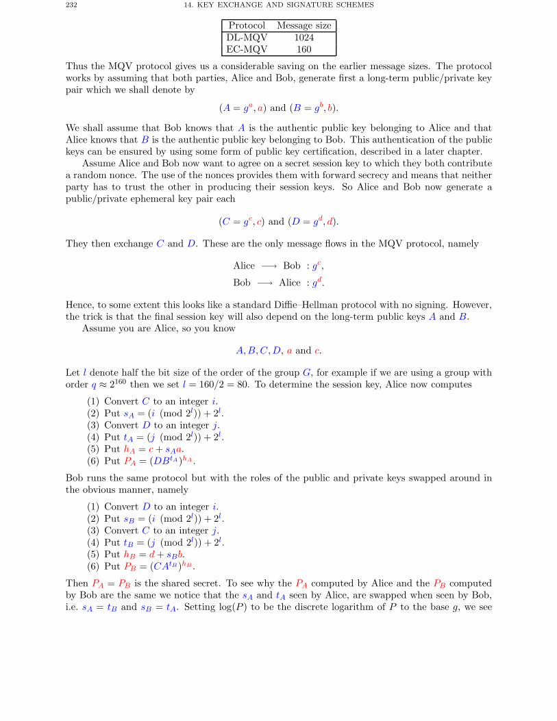
232 14. KEY EXCHANGE AND SIGNATURE SCHEMES
Protocol Message sizeDL-MQV 1024EC-MQV 160
Thus the MQV protocol gives us a considerable saving on the earlier message sizes. The protocolworks by assuming that both parties, Alice and Bob, generate first a long-term public/private keypair which we shall denote by
(A = ga, a) and (B = gb, b).
We shall assume that Bob knows that A is the authentic public key belonging to Alice and thatAlice knows that B is the authentic public key belonging to Bob. This authentication of the publickeys can be ensured by using some form of public key certification, described in a later chapter.
Assume Alice and Bob now want to agree on a secret session key to which they both contributea random nonce. The use of the nonces provides them with forward secrecy and means that neitherparty has to trust the other in producing their session keys. So Alice and Bob now generate apublic/private ephemeral key pair each
(C = gc, c) and (D = gd, d).
They then exchange C and D. These are the only message flows in the MQV protocol, namely
Alice −→ Bob : gc,
Bob −→ Alice : gd.
Hence, to some extent this looks like a standard Diffie–Hellman protocol with no signing. However,the trick is that the final session key will also depend on the long-term public keys A and B.
Assume you are Alice, so you know
A,B,C,D, a and c.
Let l denote half the bit size of the order of the group G, for example if we are using a group withorder q ≈ 2160 then we set l = 160/2 = 80. To determine the session key, Alice now computes
(1) Convert C to an integer i.(2) Put sA = (i (mod 2l)) + 2l.(3) Convert D to an integer j.(4) Put tA = (j (mod 2l)) + 2l.(5) Put hA = c+ sAa.(6) Put PA = (DBtA)hA .
Bob runs the same protocol but with the roles of the public and private keys swapped around inthe obvious manner, namely
(1) Convert D to an integer i.(2) Put sB = (i (mod 2l)) + 2l.(3) Convert C to an integer j.(4) Put tB = (j (mod 2l)) + 2l.(5) Put hB = d+ sBb.(6) Put PB = (CAtB )hB .
Then PA = PB is the shared secret. To see why the PA computed by Alice and the PB computedby Bob are the same we notice that the sA and tA seen by Alice, are swapped when seen by Bob,i.e. sA = tB and sB = tA. Setting log(P ) to be the discrete logarithm of P to the base g, we see
Further Reading 233
that
log(PA) = log((DBtA)hA
)= (d+ btA)hA= d(c+ sAa) + btA(c+ sAa)
= d(c+ tBa) + bsB(c+ tBa)
= c(d+ sBb) + atB(d+ sBb)
= (c+ atB)hB
= log((CAtB )hB
)= log(PB).
Chapter Summary
• Diffie–Hellman key exchange can be used for two parties to agree on a secret key over aninsecure channel. However, Diffie–Hellman is susceptible to the man in the middle attackand so requires some form of authentication of the communicating parties.
• Digital signatures provide authentication for both long-term and short-term purposes.They come in two variants either with message recovery or as a signature with appendix.
• The RSA encryption algorithm can be used in reverse to produce a public key signaturescheme, but one needs to combine the RSA algorithm with a hash algorithm to obtainsecurity for both short and long messages.
• DSA is a signature algorithm based on discrete logarithms, it has reduced bandwidthcompared with RSA but is slower. EC-DSA is the elliptic curve variant of DSA, it alsohas the benefit of reduced bandwidth compared to DSA, but is more efficient than DSA.
• Other discrete logarithm based signature algorithms exist, all with different properties.Two we have looked at are Schnorr signatures and Nyberg–Rueppel signatures.
• Another way of using a key exchange scheme, without the need for digital signatures, isto use the MQV system. This has very small bandwidth requirements. It obtains implicitauthentication of the agreed key, by combining the ephemeral exchanged key with thelong-term static public key of each user, so as to obtain a new session key.
Further Reading
Details on more esoteric signature schemes such as one-time signatures, fail-stop signatures andundeniable signatures can be found in the books by Stinson and Schneier. These are also goodplaces to look for further details about hash functions and message authentication codes, althoughby far the best reference in this area is HAC.
B. Schneier. Applied Cryptography. Wiley, 1996.
D. Stinson. Cryptography: Theory and Practice. CRC Press, 1995.

CHAPTER 15
Implementation Issues
Chapter Goals
• To show how exponentiation algorithms are implemented.• To explain how modular arithmetic can be implemented efficiently on large numbers.• To show how certain tricks can be used to speed up RSA and DSA operations.• To show how finite fields of characteristic two can be implemented efficiently.
1. Introduction
In this chapter we examine how one actually implements cryptographic operations. We shallmainly be concerned with public key operations since those are the most complex to implement.For example, in RSA or DSA we have to perform a modular exponentiation with respect to amodulus of a thousand or more bits. This means we need to understand the implementation issuesinvolved with both modular arithmetic and exponentiation algorithms.
There is another reason to focus on public key algorithms rather than private key ones: ingeneral public key schemes run much slower than symmetric schemes. In fact they can be so slowthat their use can seriously slow down networks and web servers. Hence, efficient implementationis crucial unless one is willing to pay a large performance penalty.
Since RSA is the easiest system to understand we will concentrate on this, although wherespecial techniques exist for other schemes we will mention these as well. The chapter focuses onalgorithms used in software, for hardware based algorithms one often uses different techniquesentirely, but these alternative techniques are related to those used in software, so an understandingof software techniques is important.
2. Exponentiation Algorithms
So far in this book we have assumed that computing
ab (mod c)
is an easy operation. We need this operation both in RSA and in systems based on discrete loga-rithms such as ElGamal encryption and DSA. In this section we concentrate on the exponentiationalgorithms and assume that we can perform modular arithmetic efficiently. In a later section weshall discuss how to perform modular arithmetic.
As we have already stressed, the main operation in RSA and DSA is modular exponentiation
M = Cd (mod N).
Firstly note it does not make sense to perform this via• compute R = Cd,• then compute R (mod N).
235
236 15. IMPLEMENTATION ISSUES
To see this, consider
1235 (mod 511) = 28 153 056 843 (mod 511) = 359.
With this naive method one obtains a huge intermediate result, in our small case above this is
28 153 056 843.
But in a real 1024-bit RSA multiplication this intermediate result would be in general
21024 · 1024bits long. Such a number requires 10301 gigabytes simply to write down.
To stop this explosion in the size of any intermediate results we use the fact that we are workingmodulo N . But even here one needs to be careful, a naive algorithm would compute the aboveexample by computing
x = 123,
x2 = x× x (mod 511) = 310,
x3 = x× x2 (mod 511) = 316,
x4 = x× x3 (mod 511) = 32,
x5 = x× x4 (mod 511) = 359.
This requires four modular multiplications, which seems fine for our small example. But for ageneral RSA exponentiation by a 1024-bit exponent using this method would require around 21024
modular multiplications. If each such multiplication could be done in under one millionth of asecond we would still require 10294 years to perform an RSA decryption operation.
However, it is easy to see that, even in our small example, we can reduce the number of requiredmultiplications by being a little more clever:
x = 123,
x2 = x× x (mod 511) = 310,
x4 = x2 × x2 (mod 511) = 32,
x5 = x× x4 (mod 511) = 359.
Which only requires three modular multiplications rather than the previous four. To understandwhy we only require three modular multiplications notice that the exponent 5 has binary represen-tation 0b101 and so
• has bit length t = 3,• has Hamming weight h = 2.
In the above example we required 1 = (h − 1) general multiplications and 2 = (t − 1) squarings.This fact holds in general, in that a modular exponentiation can be performed using
• (h− 1) multiplications,• (t− 1) squarings,
where t is the bit length of the exponent and h is the Hamming weight. The average Hammingweight of an integer is t/2 so the number of multiplications and squarings is on average
t+ t/2 − 1.
For a 1024-bit RSA modulus this means that the average number of modular multiplications neededto perform exponentiation by a 1024-bit exponent is at most 2048 and on average 1535.
The method used to achieve this improvement in performance is called the binary exponentiationmethod. This is because it works by reading each bit of the binary representation of the exponent
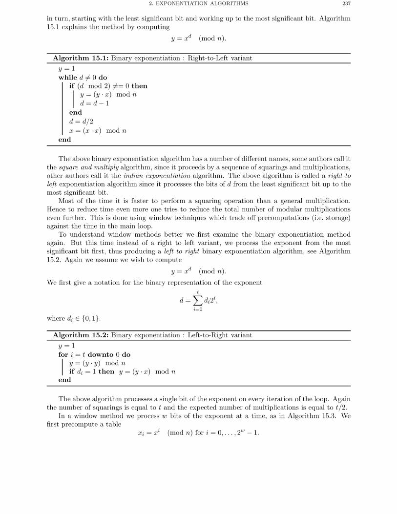
2. EXPONENTIATION ALGORITHMS 237
in turn, starting with the least significant bit and working up to the most significant bit. Algorithm15.1 explains the method by computing
y = xd (mod n).
Algorithm 15.1: Binary exponentiation : Right-to-Left varianty = 1while d �= 0 do
if (d mod 2) �== 0 theny = (y · x) mod nd = d− 1
endd = d/2x = (x · x) mod n
end
The above binary exponentiation algorithm has a number of different names, some authors call itthe square and multiply algorithm, since it proceeds by a sequence of squarings and multiplications,other authors call it the indian exponentiation algorithm. The above algorithm is called a right toleft exponentiation algorithm since it processes the bits of d from the least significant bit up to themost significant bit.
Most of the time it is faster to perform a squaring operation than a general multiplication.Hence to reduce time even more one tries to reduce the total number of modular multiplicationseven further. This is done using window techniques which trade off precomputations (i.e. storage)against the time in the main loop.
To understand window methods better we first examine the binary exponentiation methodagain. But this time instead of a right to left variant, we process the exponent from the mostsignificant bit first, thus producing a left to right binary exponentiation algorithm, see Algorithm15.2. Again we assume we wish to compute
y = xd (mod n).
We first give a notation for the binary representation of the exponent
d =t∑i=0
di2i,
where di ∈ {0, 1}.
Algorithm 15.2: Binary exponentiation : Left-to-Right varianty = 1for i = t downto 0 do
y = (y · y) mod nif di = 1 then y = (y · x) mod n
end
The above algorithm processes a single bit of the exponent on every iteration of the loop. Againthe number of squarings is equal to t and the expected number of multiplications is equal to t/2.
In a window method we process w bits of the exponent at a time, as in Algorithm 15.3. Wefirst precompute a table
xi = xi (mod n) for i = 0, . . . , 2w − 1.
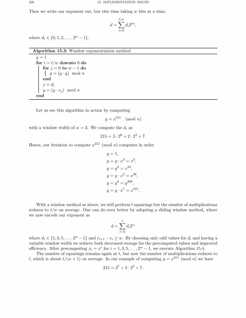
238 15. IMPLEMENTATION ISSUES
Then we write our exponent out, but this time taking w bits at a time,
d =t/w∑i=0
di2iw,
where di ∈ {0, 1, 2, . . . , 2w − 1}.
Algorithm 15.3: Window exponentiation methody = 1for i = t/w downto 0 do
for j = 0 to w − 1 doy = (y · y) mod n
endj = diy = (y · xj) mod n
end
Let us see this algorithm in action by computing
y = x215 (mod n)
with a window width of w = 3. We compute the di as
215 = 3 · 26 + 2 · 23 + 7.
Hence, our iteration to compute x215 (mod n) computes in order
y = 1,
y = y · x3 = x3,
y = y8 = x24,
y = y · x2 = x26,
y = y8 = y208,
y = y · x7 = x215.
With a window method as above, we still perform t squarings but the number of multiplicationsreduces to t/w on average. One can do even better by adopting a sliding window method, wherewe now encode our exponent as
d =l∑
i=0
di2ei
where di ∈ {1, 3, 5, . . . , 2w − 1} and ei+1 − ei ≥ w. By choosing only odd values for di and having avariable window width we achieve both decreased storage for the precomputed values and improvedefficiency. After precomputing xi = xi for i = 1, 3, 5, . . . , 2w − 1, we execute Algorithm 15.4.
The number of squarings remains again at t, but now the number of multiplications reduces tol, which is about t/(w + 1) on average. In our example of computing y = x215 (mod n) we have
215 = 27 + 5 · 24 + 7,
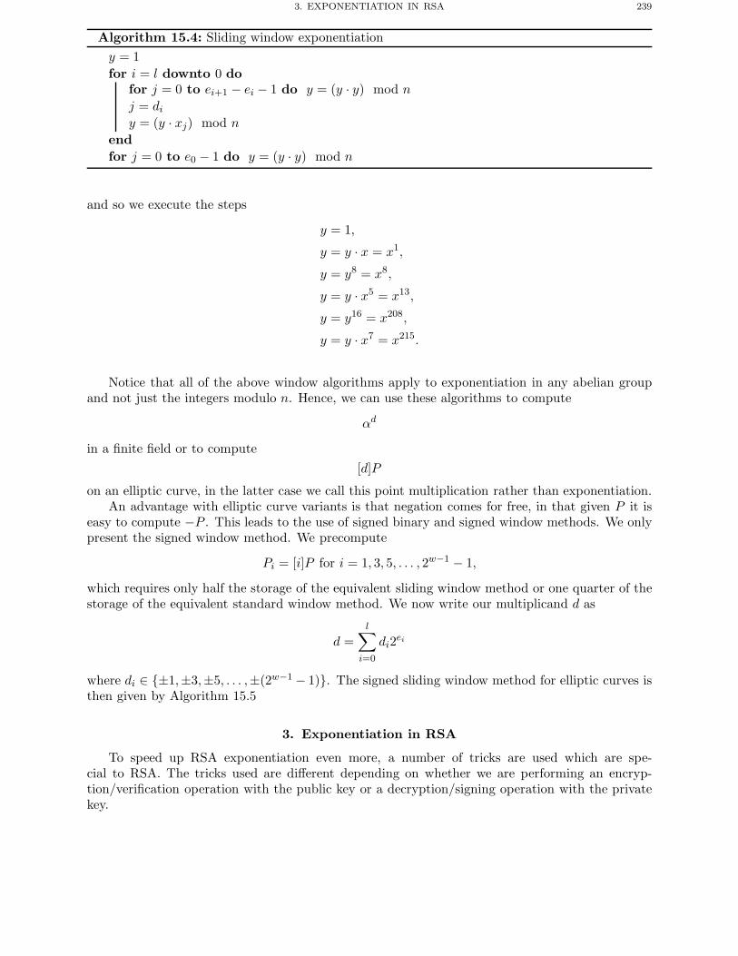
3. EXPONENTIATION IN RSA 239
Algorithm 15.4: Sliding window exponentiationy = 1for i = l downto 0 do
for j = 0 to ei+1 − ei − 1 do y = (y · y) mod nj = diy = (y · xj) mod n
endfor j = 0 to e0 − 1 do y = (y · y) mod n
and so we execute the steps
y = 1,
y = y · x = x1,
y = y8 = x8,
y = y · x5 = x13,
y = y16 = x208,
y = y · x7 = x215.
Notice that all of the above window algorithms apply to exponentiation in any abelian groupand not just the integers modulo n. Hence, we can use these algorithms to compute
αd
in a finite field or to compute[d]P
on an elliptic curve, in the latter case we call this point multiplication rather than exponentiation.An advantage with elliptic curve variants is that negation comes for free, in that given P it is
easy to compute −P . This leads to the use of signed binary and signed window methods. We onlypresent the signed window method. We precompute
Pi = [i]P for i = 1, 3, 5, . . . , 2w−1 − 1,
which requires only half the storage of the equivalent sliding window method or one quarter of thestorage of the equivalent standard window method. We now write our multiplicand d as
d =l∑
i=0
di2ei
where di ∈ {±1,±3,±5, . . . ,±(2w−1 − 1)}. The signed sliding window method for elliptic curves isthen given by Algorithm 15.5
3. Exponentiation in RSA
To speed up RSA exponentiation even more, a number of tricks are used which are spe-cial to RSA. The tricks used are different depending on whether we are performing an encryp-tion/verification operation with the public key or a decryption/signing operation with the privatekey.
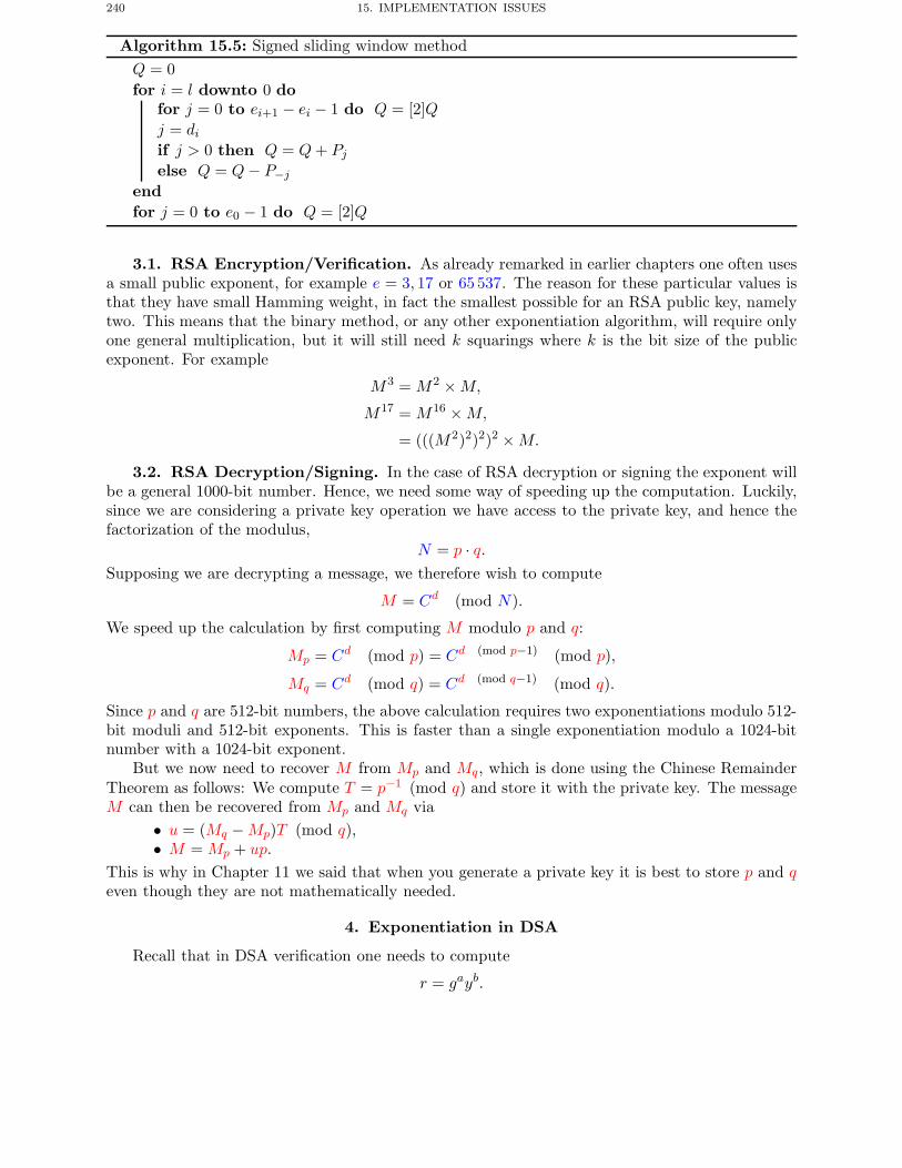
240 15. IMPLEMENTATION ISSUES
Algorithm 15.5: Signed sliding window methodQ = 0for i = l downto 0 do
for j = 0 to ei+1 − ei − 1 do Q = [2]Qj = diif j > 0 then Q = Q+ Pjelse Q = Q− P−j
endfor j = 0 to e0 − 1 do Q = [2]Q
3.1. RSA Encryption/Verification. As already remarked in earlier chapters one often usesa small public exponent, for example e = 3, 17 or 65 537. The reason for these particular values isthat they have small Hamming weight, in fact the smallest possible for an RSA public key, namelytwo. This means that the binary method, or any other exponentiation algorithm, will require onlyone general multiplication, but it will still need k squarings where k is the bit size of the publicexponent. For example
M3 = M2 ×M,
M17 = M16 ×M,
= (((M2)2)2)2 ×M.
3.2. RSA Decryption/Signing. In the case of RSA decryption or signing the exponent willbe a general 1000-bit number. Hence, we need some way of speeding up the computation. Luckily,since we are considering a private key operation we have access to the private key, and hence thefactorization of the modulus,
N = p · q.Supposing we are decrypting a message, we therefore wish to compute
M = Cd (mod N).
We speed up the calculation by first computing M modulo p and q:
Mp = Cd (mod p) = Cd (mod p−1) (mod p),
Mq = Cd (mod q) = Cd (mod q−1) (mod q).
Since p and q are 512-bit numbers, the above calculation requires two exponentiations modulo 512-bit moduli and 512-bit exponents. This is faster than a single exponentiation modulo a 1024-bitnumber with a 1024-bit exponent.
But we now need to recover M from Mp and Mq, which is done using the Chinese RemainderTheorem as follows: We compute T = p−1 (mod q) and store it with the private key. The messageM can then be recovered from Mp and Mq via
• u = (Mq −Mp)T (mod q),• M = Mp + up.
This is why in Chapter 11 we said that when you generate a private key it is best to store p and qeven though they are not mathematically needed.
4. Exponentiation in DSA
Recall that in DSA verification one needs to compute
r = gayb.
5. MULTI-PRECISION ARITHMETIC 241
This can be accomplished by first computing ga and then yb and then multiplying the resultstogether. However, often it is easier to perform the two exponentiations simultaneously. There area number of techniques to accomplish this, using various forms of window techniques etc. But allare essentially based on the following idea, called Shamir’s trick.
We first compute the following look-up table
Gi = gi0yi1
where i = (i1, i0) is the binary representation of i, for i = 0, 1, 2, 3. We then compute an exponentarray from the two exponents a and b. This is a 2 by t array, where t is the maximum bit length ofa and b. The rows of this array are the binary representation of the exponents a and b. We thenlet Ij, for j = 1, . . . , t, denote the integers whose binary representation is given by the columns ofthis array. The exponentiation is then computed by setting r = 1 and computing
r = r2 ·GIjfor j = 1 to t.
As an example suppose we wish to compute
r = g11y7,
hence we have t = 4. We precompute
G0 = 1, G1 = g, G2 = y, G3 = g · y.Since the binary representation of 11 and 7 is given by 1011 and 111, our exponent array is givenby (
1 0 1 10 1 1 1
).
The integers Ij then becomeI1 = 1, I2 = 2, I3 = 3, I4 = 3.
Hence, the four steps of our algorithm become
r = G1 = g,
r = r2 ·G2 = g2 · y,r = r2 ·G3 = (g4 · y2) · (g · y) = g5 · y3,
r = r2 ·G3 = (g10 · y6) · (g · y) = g11 · y7.
Note, elliptic curve analogues of Shamir’s trick and its variants can be made which make use ofsigned representations for the exponent. We do not give these here, but leave them for the interestedreader to investigate.
5. Multi-precision Arithmetic
We shall now explain how to perform modular arithmetic on 1024-bit numbers. We show howthis is accomplished using modern processors, and why naive algorithms are usually replaced witha special technique due to Montgomery.
In a cryptographic application it is common to focus on a fixed length for the integers in use,for example 1024 bits in an RSA/DSA implementation or 200 bits for an ECC implementation.This leads to different programming choices than when one implements a general purpose multi-precision arithmetic library. For example one no longer needs to worry so much about dynamicmemory allocation, and one can now concentrate on particular performance enhancements for theinteger sizes one is dealing with.
It is common to represent all integers in little-wordian format. This means that if a large integeris held in memory locations, x0, x1, . . . , xn, then x0 is the least significant word and xn is the most
242 15. IMPLEMENTATION ISSUES
significant word. For a 32-bit machine and 64-bit numbers we would represent x and y as [x0, x1]and [y0, y1] where
x = x1232 + x0,
y = y1232 + y0.5.1. Addition. Most modern processors have a carry flag which is set by any overflow froman addition operation. Also most have a special instruction, usually called something like addc,which adds two integers together and adds on the contents of the carry flag. So if we wish to addour two 64-bit integers given earlier then we need to compute
z = x+ y = z2264 + z1232 + z0.
The values of z0, z1 and z2 are then computed viaz0 <- add x0,y0z1 <- addc x1,y1z2 <- addc 0,0
Note that the value held in z2 is at most one, so the value of z could be a 65-bit integer. Theabove technique for adding two 64-bit integers can clearly be scaled to adding integers of any fixedlength, and can also be made to work for subtraction of large integers.
5.2. School-book Multiplication. We now turn to the next simplest arithmetic operation,after addition and subtraction, namely multiplication. Notice that two 32 -bit words multiplytogether to form a 64-bit result, and so most modern processors have an instruction which will dothis operation.
w1 · w2 = (High,Low) = (H(w1 · w2), L(w1 · w2)).When we use school-book long multiplication, for our two 64-bit numbers, we obtain somethinglike
x1 x0
× y1 y0
H(x0 · y0) L(x0 · y0)H(x0 · y1) L(x0 · y1)H(x1 · y0) L(x1 · y0)
H(x1 · y1) L(x1 · y1)Then we add up the four rows to get the answer, remembering we need to take care of the carries.This then becomes, for
z = x · y,something like the following pseudo-code
(z1,z0) <- mul x0,y0(z3,z2) <- mul x1,y1(h,l) <- mul x1,y0z1 <- add z1,lz2 <- addc z2,hz3 <- addc z3,0(h,l) <- mul x0,y1z1 <- add z1,lz2 <- addc z2,hz3 <- addc z3,0
If n denotes the bit size of the integers we are operating on, the above technique for multiplyinglarge integers together clearly requires O(n2) bit operations, whilst it requires O(n) bit operationsto add or subtract integers. It is a natural question as to whether one can multiply integers fasterthan O(n2).
5. MULTI-PRECISION ARITHMETIC 243
5.3. Karatsuba Multiplication. One technique to speed up multiplication is called Karat-suba multiplication. Suppose we have two n-bit integers x and y that we wish to multiply. Wewrite these integers as
x = x0 + 2n/2x1,
y = y0 + 2n/2y2,
where 0 ≤ x0, x1, y0, y1 < 2n/2. We then multiply x and y by computing
A = x0 · y0,
B = (x0 + x1) · (y0 + y1),C = x1 · y1.
The product x · y is then given by
C2n + (B −A−C)2n/2 +A = x1y12n + (x1y0 + x0y1)2n/2 + x0y0
= (x0 + 2n/2x1) · (y0 + 2n/2y1)= x · y.
Hence, this multiplication technique to multiply two n-bit numbers requires three n/2-bit multi-plications, two n/2-bit additions and three n-bit additions/subtractions. If we denote the cost ofan n-bit multiplication by M(n) and the cost of an n-bit addition/subtraction by A(n) then thisbecomes
M(n) = 3M(n/2) + 2A(n/2) + 3A(n).
Now if we make the approximation that A(n) ≈ n then
M(n) ≈ 3M(n/2) + 4n.
If the multiplication of the n/2-bit numbers is accomplished in a similar fashion then to obtain thefinal complexity of multiplication we need to solve the above recurrence relation to obtain
M(n) ≈ 9nlog(3)log(2) as n −→ ∞
= 9n1.58.
So we obtain an algorithm with asymptotic complexity O(n1.58). Karatsuba multiplication becomesfaster than the O(n2) method for integers of sizes greater than a few hundred bits. However, onecan do even better for very large integers since the fastest known multiplication algorithm takestime
O(n log n log log n).
But neither this latter technique nor Karatsuba multiplication are used in many cryptographicapplications. The reason for this will become apparent as we discuss integer division.
5.4. Division. After having looked at multiplication we are left with the division operation,which is the hardest of all the basic algorithms. Division is required in order to be able to computethe remainder on division, which is after all a basic operation in RSA. Given two large integers xand y we wish to be able to compute q and r such that
x = qy + r
where 0 ≤ r < y, such an operation is called a Euclidean division.If we write our two integers x and y in the little-wordian format
x = (x0, . . . , xn) and y = (y0, . . . , yt)
244 15. IMPLEMENTATION ISSUES
where the base for the representation is b = 2w then the Euclidean division can be performed byAlgorithm 15.6. We let t �w v denote a large integer t shifted to the left by v words, in otherwords the result of multiplying t by bv.
As one can see this is a complex operation, hence one should try and avoid divisions as muchas possible.
5.5. Montgomery Arithmetic. That division is a complex operation means our crypto-graphic operations run very slowly if we use standard division operations as above. Recall thatvirtually all of our public key systems make use of arithmetic modulo another number. What werequire is the ability to compute remainders (i.e. to perform modular arithmetic) without havingto perform any costly division operations. This at first sight may seem a state of affairs which isimpossible to reach, but it can be achieved using a special form of arithmetic called Montgomeryarithmetic.
Montgomery arithmetic works by using an alternative representation of integers, called theMontgomery representation. Let us fix some notation, we let b denote 2 to the power of the wordsize of our computer, for example b = 232 or 264. To perform arithmetic modulo N we choose aninteger R which satisfies
R = bt > N.
Now instead of holding the value of the integer x in memory, we instead hold the value
x · R (mod N).
Again this is usually held in a little-wordian format. The value x ·R (mod N) is called the Mont-gomery representation of the integer x (mod N).
Adding two elements in Montgomery representation is easy. If
z = x+ y (mod N)
then given x ·R (mod N) and y ·R (mod N) we need to compute z ·R (mod N).Let us take a simple example with
N = 1073 741 827,
b = R = 232 = 4294 967 296.
The following is the map from the normal to Montgomery representation of the integers 1, 2 and 3.
1 −→ 1 ·R (mod N) = 1 073 741 815,
2 −→ 2 ·R (mod N) = 1 073 741 803,
3 −→ 3 ·R (mod N) = 1 073 741 791.
We can now verify that addition works since we have in the standard representation
1 + 2 = 3
whilst this is mirrored in the Montgomery representation as
1 073 741 815 + 1073 741 803 = 1073 741 791 (mod N).
Now we look at multiplication in Montgomery arithmetic. If we simply multiply two elementsin Montgomery representation we will obtain
(xR) · (yR) = xyR2 (mod N)
but we want xyR (mod N). Hence, we need to divide the result of the standard multiplication byR. Since R is a power of 2 we hope this should be easy.
The process of given y and computing
z = y/R (mod N)
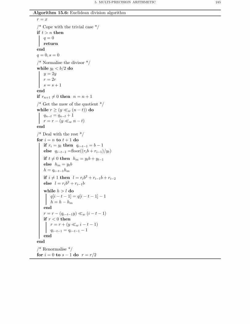
5. MULTI-PRECISION ARITHMETIC 245
Algorithm 15.6: Euclidean division algorithmr = x
/* Cope with the trivial case */if t > n then
q = 0return
endq = 0, s = 0
/* Normalise the divisor */while yt < b/2 do
y = 2yr = 2rs = s+ 1
endif rn+1 �= 0 then n = n+ 1
/* Get the msw of the quotient */while r ≥ (y �w (n− t)) do
qn−t = qn−t + 1r = r − (y �w n− t)
end
/* Deal with the rest */for i = n to t+ 1 do
if ri = yt then qi−t−1 = b− 1else qi−t−1 =floor((rib+ ri−1)/yt)
if t �= 0 then hm = ytb+ yt−1
else hm = ytb
h = qi−t−1hm
if i �= 1 then l = rib2 + ri−1b+ ri−2
else l = rib2 + ri−1b
while h > l doq[i− t− 1] = q[i− t− 1] − 1h = h− hm
endr = r − (qi−t−1y) �w (i− t− 1)if r < 0 then
r = r + (y �w i− t− 1)qi−t−1 = qi−t−1 − 1
endend
/* Renormalise */for i = 0 to s− 1 do r = r/2
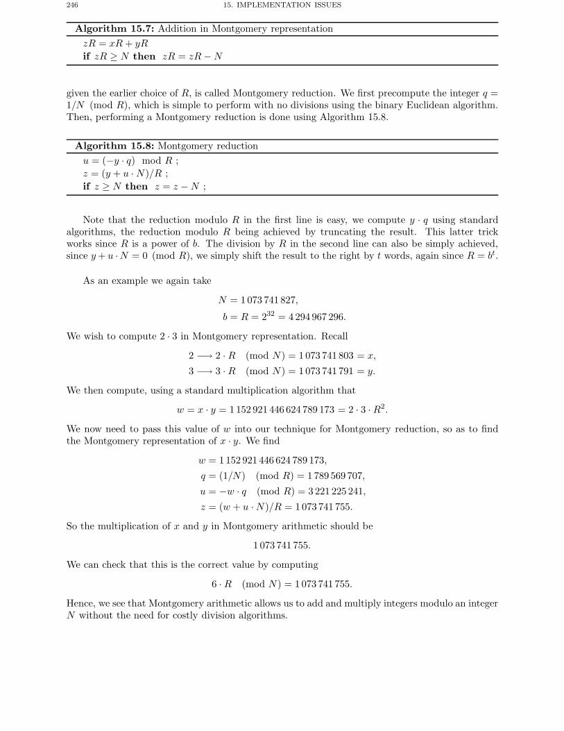
246 15. IMPLEMENTATION ISSUES
Algorithm 15.7: Addition in Montgomery representationzR = xR+ yR
if zR ≥ N then zR = zR−N
given the earlier choice of R, is called Montgomery reduction. We first precompute the integer q =1/N (mod R), which is simple to perform with no divisions using the binary Euclidean algorithm.Then, performing a Montgomery reduction is done using Algorithm 15.8.
Algorithm 15.8: Montgomery reductionu = (−y · q) mod R ;z = (y + u ·N)/R ;if z ≥ N then z = z −N ;
Note that the reduction modulo R in the first line is easy, we compute y · q using standardalgorithms, the reduction modulo R being achieved by truncating the result. This latter trickworks since R is a power of b. The division by R in the second line can also be simply achieved,since y+ u ·N = 0 (mod R), we simply shift the result to the right by t words, again since R = bt.
As an example we again take
N = 1073 741 827,
b = R = 232 = 4294 967 296.
We wish to compute 2 · 3 in Montgomery representation. Recall
2 −→ 2 · R (mod N) = 1 073 741 803 = x,
3 −→ 3 · R (mod N) = 1 073 741 791 = y.
We then compute, using a standard multiplication algorithm that
w = x · y = 1152 921 446 624 789 173 = 2 · 3 ·R2.
We now need to pass this value of w into our technique for Montgomery reduction, so as to findthe Montgomery representation of x · y. We find
w = 1152 921 446 624 789 173,
q = (1/N) (mod R) = 1 789 569 707,
u = −w · q (mod R) = 3 221 225 241,
z = (w + u ·N)/R = 1073 741 755.
So the multiplication of x and y in Montgomery arithmetic should be
1 073 741 755.
We can check that this is the correct value by computing
6 · R (mod N) = 1 073 741 755.
Hence, we see that Montgomery arithmetic allows us to add and multiply integers modulo an integerN without the need for costly division algorithms.
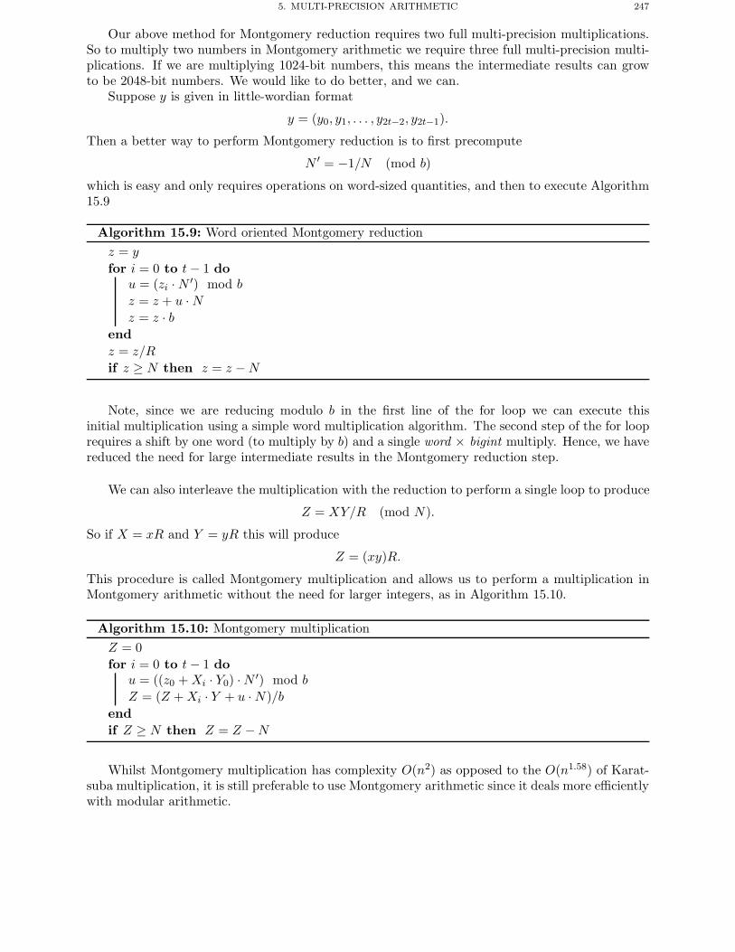
5. MULTI-PRECISION ARITHMETIC 247
Our above method for Montgomery reduction requires two full multi-precision multiplications.So to multiply two numbers in Montgomery arithmetic we require three full multi-precision multi-plications. If we are multiplying 1024-bit numbers, this means the intermediate results can growto be 2048-bit numbers. We would like to do better, and we can.
Suppose y is given in little-wordian format
y = (y0, y1, . . . , y2t−2, y2t−1).
Then a better way to perform Montgomery reduction is to first precompute
N ′ = −1/N (mod b)
which is easy and only requires operations on word-sized quantities, and then to execute Algorithm15.9
Algorithm 15.9: Word oriented Montgomery reductionz = y
for i = 0 to t− 1 dou = (zi ·N ′) mod bz = z + u ·Nz = z · b
endz = z/R
if z ≥ N then z = z −N
Note, since we are reducing modulo b in the first line of the for loop we can execute thisinitial multiplication using a simple word multiplication algorithm. The second step of the for looprequires a shift by one word (to multiply by b) and a single word × bigint multiply. Hence, we havereduced the need for large intermediate results in the Montgomery reduction step.
We can also interleave the multiplication with the reduction to perform a single loop to produce
Z = XY/R (mod N).
So if X = xR and Y = yR this will produce
Z = (xy)R.
This procedure is called Montgomery multiplication and allows us to perform a multiplication inMontgomery arithmetic without the need for larger integers, as in Algorithm 15.10.
Algorithm 15.10: Montgomery multiplicationZ = 0for i = 0 to t− 1 do
u = ((z0 +Xi · Y0) ·N ′) mod bZ = (Z +Xi · Y + u ·N)/b
endif Z ≥ N then Z = Z −N
Whilst Montgomery multiplication has complexity O(n2) as opposed to the O(n1.58) of Karat-suba multiplication, it is still preferable to use Montgomery arithmetic since it deals more efficientlywith modular arithmetic.
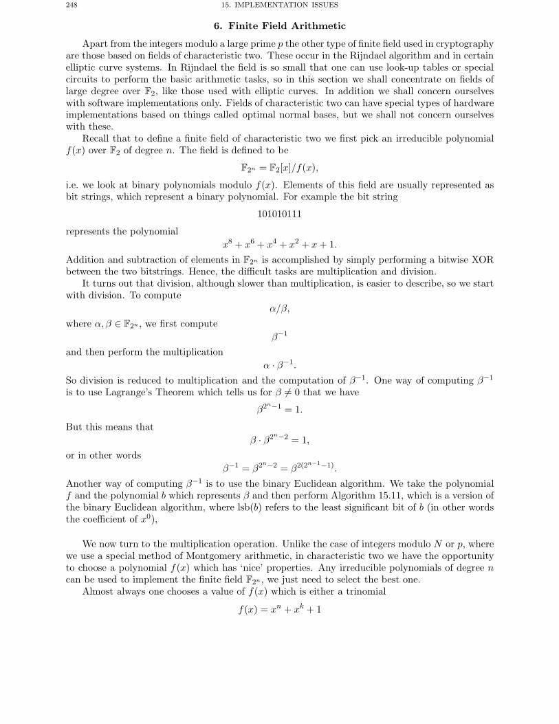
248 15. IMPLEMENTATION ISSUES
6. Finite Field Arithmetic
Apart from the integers modulo a large prime p the other type of finite field used in cryptographyare those based on fields of characteristic two. These occur in the Rijndael algorithm and in certainelliptic curve systems. In Rijndael the field is so small that one can use look-up tables or specialcircuits to perform the basic arithmetic tasks, so in this section we shall concentrate on fields oflarge degree over F2, like those used with elliptic curves. In addition we shall concern ourselveswith software implementations only. Fields of characteristic two can have special types of hardwareimplementations based on things called optimal normal bases, but we shall not concern ourselveswith these.
Recall that to define a finite field of characteristic two we first pick an irreducible polynomialf(x) over F2 of degree n. The field is defined to be
F2n = F2[x]/f(x),
i.e. we look at binary polynomials modulo f(x). Elements of this field are usually represented asbit strings, which represent a binary polynomial. For example the bit string
101010111
represents the polynomialx8 + x6 + x4 + x2 + x+ 1.
Addition and subtraction of elements in F2n is accomplished by simply performing a bitwise XORbetween the two bitstrings. Hence, the difficult tasks are multiplication and division.
It turns out that division, although slower than multiplication, is easier to describe, so we startwith division. To compute
α/β,
where α, β ∈ F2n , we first computeβ−1
and then perform the multiplicationα · β−1.
So division is reduced to multiplication and the computation of β−1. One way of computing β−1
is to use Lagrange’s Theorem which tells us for β �= 0 that we have
β2n−1 = 1.
But this means thatβ · β2n−2 = 1,
or in other wordsβ−1 = β2n−2 = β2(2n−1−1).
Another way of computing β−1 is to use the binary Euclidean algorithm. We take the polynomialf and the polynomial b which represents β and then perform Algorithm 15.11, which is a version ofthe binary Euclidean algorithm, where lsb(b) refers to the least significant bit of b (in other wordsthe coefficient of x0),
We now turn to the multiplication operation. Unlike the case of integers modulo N or p, wherewe use a special method of Montgomery arithmetic, in characteristic two we have the opportunityto choose a polynomial f(x) which has ‘nice’ properties. Any irreducible polynomials of degree ncan be used to implement the finite field F2n , we just need to select the best one.
Almost always one chooses a value of f(x) which is either a trinomial
f(x) = xn + xk + 1
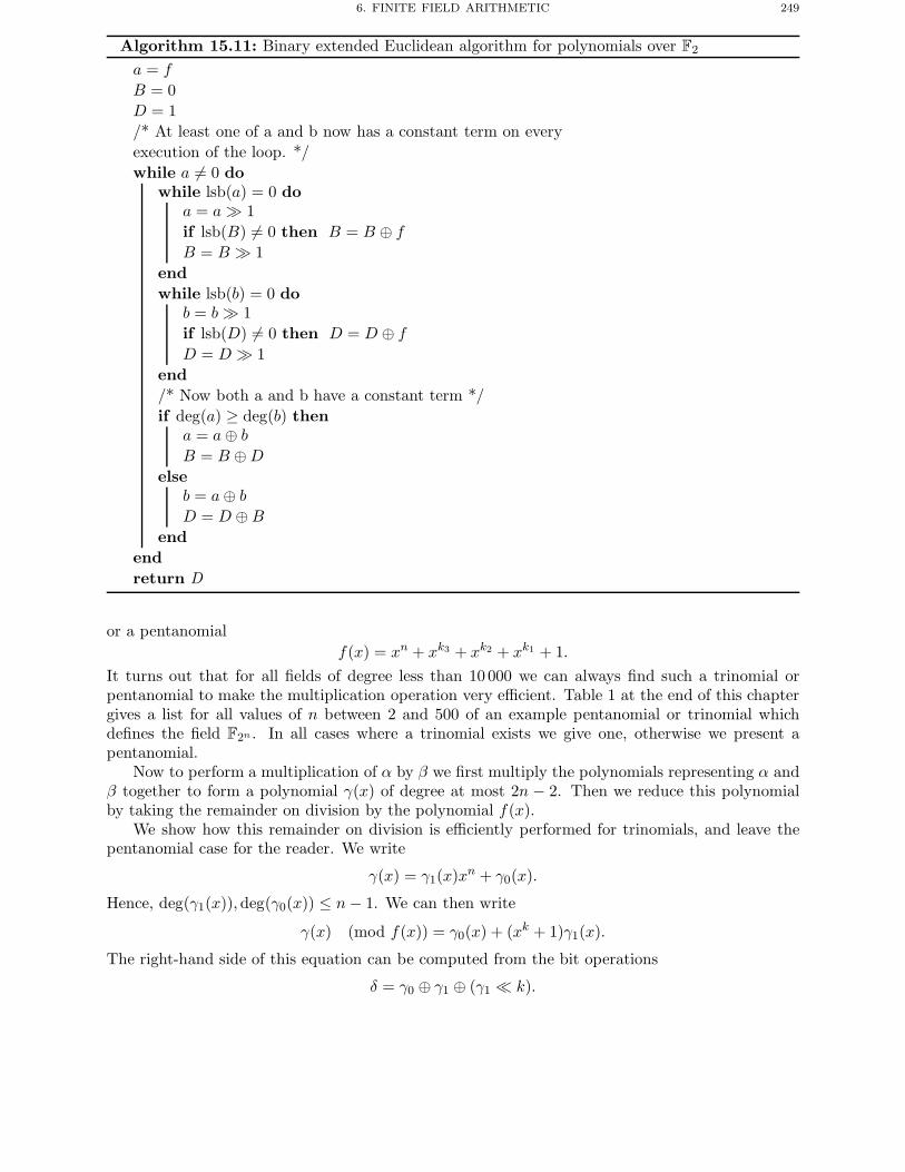
6. FINITE FIELD ARITHMETIC 249
Algorithm 15.11: Binary extended Euclidean algorithm for polynomials over F2
a = f
B = 0D = 1/* At least one of a and b now has a constant term on everyexecution of the loop. */while a �= 0 do
while lsb(a) = 0 doa = a� 1if lsb(B) �= 0 then B = B ⊕ f
B = B � 1endwhile lsb(b) = 0 do
b = b� 1if lsb(D) �= 0 then D = D ⊕ f
D = D � 1end/* Now both a and b have a constant term */if deg(a) ≥ deg(b) then
a = a⊕ b
B = B ⊕D
elseb = a⊕ b
D = D ⊕B
endendreturn D
or a pentanomialf(x) = xn + xk3 + xk2 + xk1 + 1.
It turns out that for all fields of degree less than 10 000 we can always find such a trinomial orpentanomial to make the multiplication operation very efficient. Table 1 at the end of this chaptergives a list for all values of n between 2 and 500 of an example pentanomial or trinomial whichdefines the field F2n . In all cases where a trinomial exists we give one, otherwise we present apentanomial.
Now to perform a multiplication of α by β we first multiply the polynomials representing α andβ together to form a polynomial γ(x) of degree at most 2n − 2. Then we reduce this polynomialby taking the remainder on division by the polynomial f(x).
We show how this remainder on division is efficiently performed for trinomials, and leave thepentanomial case for the reader. We write
γ(x) = γ1(x)xn + γ0(x).
Hence, deg(γ1(x)),deg(γ0(x)) ≤ n− 1. We can then write
γ(x) (mod f(x)) = γ0(x) + (xk + 1)γ1(x).
The right-hand side of this equation can be computed from the bit operations
δ = γ0 ⊕ γ1 ⊕ (γ1 � k).
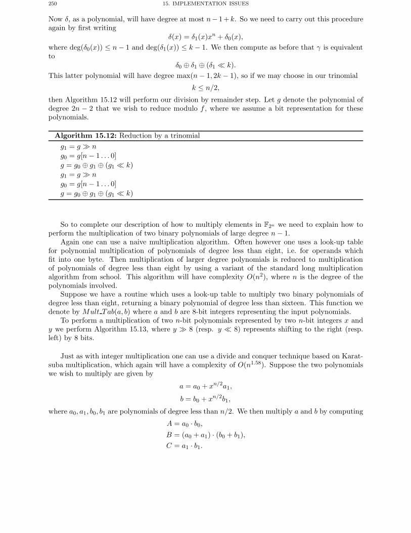
250 15. IMPLEMENTATION ISSUES
Now δ, as a polynomial, will have degree at most n− 1+ k. So we need to carry out this procedureagain by first writing
δ(x) = δ1(x)xn + δ0(x),where deg(δ0(x)) ≤ n− 1 and deg(δ1(x)) ≤ k − 1. We then compute as before that γ is equivalentto
δ0 ⊕ δ1 ⊕ (δ1 � k).This latter polynomial will have degree max(n− 1, 2k − 1), so if we may choose in our trinomial
k ≤ n/2,
then Algorithm 15.12 will perform our division by remainder step. Let g denote the polynomial ofdegree 2n − 2 that we wish to reduce modulo f , where we assume a bit representation for thesepolynomials.
Algorithm 15.12: Reduction by a trinomialg1 = g � n
g0 = g[n − 1 . . . 0]g = g0 ⊕ g1 ⊕ (g1 � k)g1 = g � n
g0 = g[n − 1 . . . 0]g = g0 ⊕ g1 ⊕ (g1 � k)
So to complete our description of how to multiply elements in F2n we need to explain how toperform the multiplication of two binary polynomials of large degree n− 1.
Again one can use a naive multiplication algorithm. Often however one uses a look-up tablefor polynomial multiplication of polynomials of degree less than eight, i.e. for operands whichfit into one byte. Then multiplication of larger degree polynomials is reduced to multiplicationof polynomials of degree less than eight by using a variant of the standard long multiplicationalgorithm from school. This algorithm will have complexity O(n2), where n is the degree of thepolynomials involved.
Suppose we have a routine which uses a look-up table to multiply two binary polynomials ofdegree less than eight, returning a binary polynomial of degree less than sixteen. This function wedenote by Mult Tab(a, b) where a and b are 8-bit integers representing the input polynomials.
To perform a multiplication of two n-bit polynomials represented by two n-bit integers x andy we perform Algorithm 15.13, where y � 8 (resp. y � 8) represents shifting to the right (resp.left) by 8 bits.
Just as with integer multiplication one can use a divide and conquer technique based on Karat-suba multiplication, which again will have a complexity of O(n1.58). Suppose the two polynomialswe wish to multiply are given by
a = a0 + xn/2a1,
b = b0 + xn/2b1,
where a0, a1, b0, b1 are polynomials of degree less than n/2. We then multiply a and b by computing
A = a0 · b0,B = (a0 + a1) · (b0 + b1),C = a1 · b1.
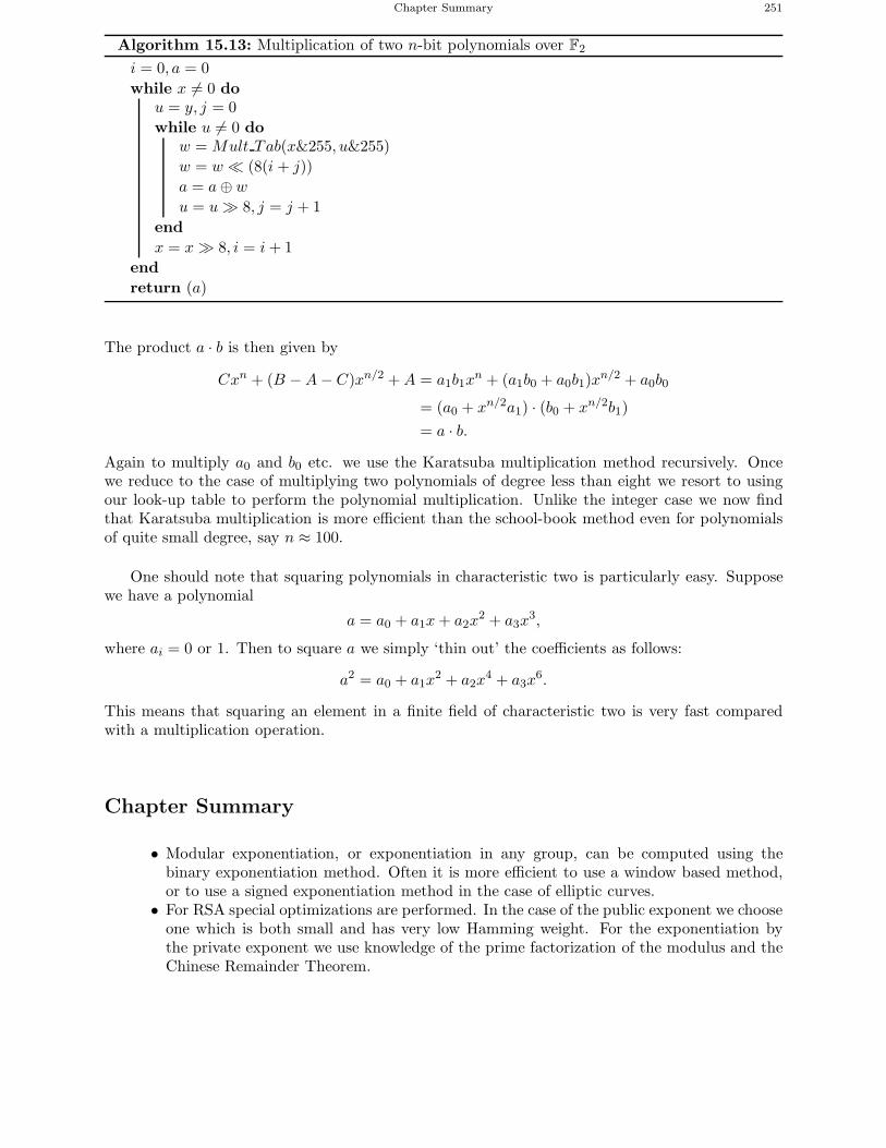
Chapter Summary 251
Algorithm 15.13: Multiplication of two n-bit polynomials over F2
i = 0, a = 0while x �= 0 do
u = y, j = 0while u �= 0 do
w = Mult Tab(x&255, u&255)w = w � (8(i + j))a = a⊕ w
u = u� 8, j = j + 1endx = x� 8, i = i+ 1
endreturn (a)
The product a · b is then given by
Cxn + (B −A− C)xn/2 +A = a1b1xn + (a1b0 + a0b1)xn/2 + a0b0
= (a0 + xn/2a1) · (b0 + xn/2b1)= a · b.
Again to multiply a0 and b0 etc. we use the Karatsuba multiplication method recursively. Oncewe reduce to the case of multiplying two polynomials of degree less than eight we resort to usingour look-up table to perform the polynomial multiplication. Unlike the integer case we now findthat Karatsuba multiplication is more efficient than the school-book method even for polynomialsof quite small degree, say n ≈ 100.
One should note that squaring polynomials in characteristic two is particularly easy. Supposewe have a polynomial
a = a0 + a1x+ a2x2 + a3x
3,
where ai = 0 or 1. Then to square a we simply ‘thin out’ the coefficients as follows:
a2 = a0 + a1x2 + a2x
4 + a3x6.
This means that squaring an element in a finite field of characteristic two is very fast comparedwith a multiplication operation.
Chapter Summary
• Modular exponentiation, or exponentiation in any group, can be computed using thebinary exponentiation method. Often it is more efficient to use a window based method,or to use a signed exponentiation method in the case of elliptic curves.
• For RSA special optimizations are performed. In the case of the public exponent we chooseone which is both small and has very low Hamming weight. For the exponentiation bythe private exponent we use knowledge of the prime factorization of the modulus and theChinese Remainder Theorem.
252 15. IMPLEMENTATION ISSUES
• For DSA verification there is a method based on simultaneous exponentiation which isoften more efficient than performing two single exponentiations and then combining theresult.
• Modular arithmetic is usually implemented using the technique of Montgomery represen-tation. This allows us to avoid costly division operations by replacing the division withsimple shift operations. This however is at the expense of using a non-standard represen-tation for the numbers.
• Finite fields in characteristic two can also be implemented efficiently. But now the modularreduction operation can be made simple by choosing a special polynomial f(x). Inversionis also particular simple using a variant of the binary Euclidean algorithm, although ofteninversion is still 3–10 times slower than multiplication.
Further Reading
The standard reference work for the type of algorithms considered in this chapter is Volume 2of Knuth. A more gentle introduction can be found in the book by Bach and Shallit, whilst formore algorithms one should consult the book by Cohen. The first chapter of Cohen gives a numberof lessons learnt in the development of the PARI/GP calculator which can be useful, whilst Bachand Shallit provides an extensive bibliography and associated commentary.
E. Bach and S. Shallit. Algorithmic Number Theory, Volume 1: Efficient Algorithms. MIT Press,1996.
H. Cohen. A Course in Computational Algebraic Number Theory. Springer-Verlag, 1993.
D. Knuth. The Art of Computing Programming, Volume 2 : Seminumerical Algorithms. Addison-Wesley, 1975.
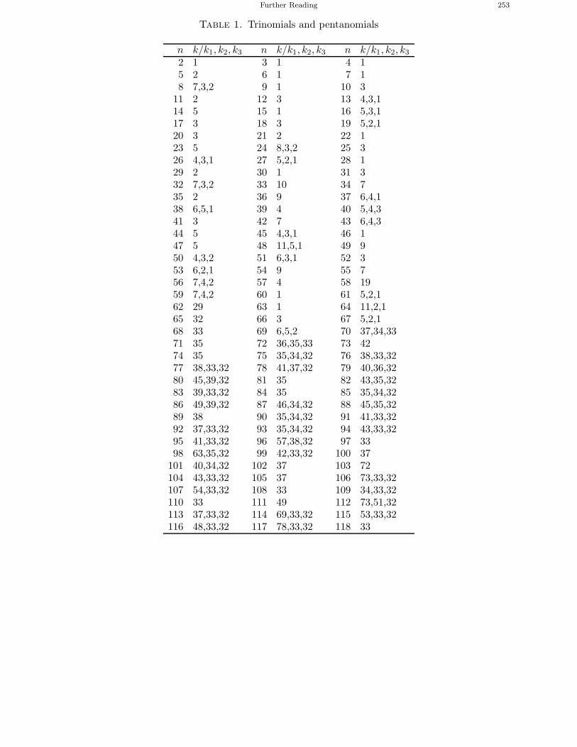
Further Reading 253
Table 1. Trinomials and pentanomials
n k/k1, k2, k3 n k/k1, k2, k3 n k/k1, k2, k3
2 1 3 1 4 15 2 6 1 7 18 7,3,2 9 1 10 3
11 2 12 3 13 4,3,114 5 15 1 16 5,3,117 3 18 3 19 5,2,120 3 21 2 22 123 5 24 8,3,2 25 326 4,3,1 27 5,2,1 28 129 2 30 1 31 332 7,3,2 33 10 34 735 2 36 9 37 6,4,138 6,5,1 39 4 40 5,4,341 3 42 7 43 6,4,344 5 45 4,3,1 46 147 5 48 11,5,1 49 950 4,3,2 51 6,3,1 52 353 6,2,1 54 9 55 756 7,4,2 57 4 58 1959 7,4,2 60 1 61 5,2,162 29 63 1 64 11,2,165 32 66 3 67 5,2,168 33 69 6,5,2 70 37,34,3371 35 72 36,35,33 73 4274 35 75 35,34,32 76 38,33,3277 38,33,32 78 41,37,32 79 40,36,3280 45,39,32 81 35 82 43,35,3283 39,33,32 84 35 85 35,34,3286 49,39,32 87 46,34,32 88 45,35,3289 38 90 35,34,32 91 41,33,3292 37,33,32 93 35,34,32 94 43,33,3295 41,33,32 96 57,38,32 97 3398 63,35,32 99 42,33,32 100 37
101 40,34,32 102 37 103 72104 43,33,32 105 37 106 73,33,32107 54,33,32 108 33 109 34,33,32110 33 111 49 112 73,51,32113 37,33,32 114 69,33,32 115 53,33,32116 48,33,32 117 78,33,32 118 33
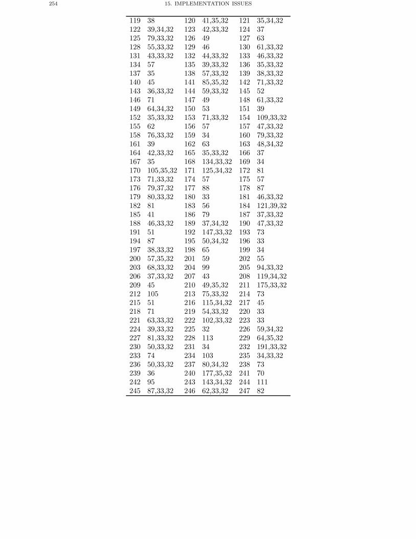
254 15. IMPLEMENTATION ISSUES
119 38 120 41,35,32 121 35,34,32122 39,34,32 123 42,33,32 124 37125 79,33,32 126 49 127 63128 55,33,32 129 46 130 61,33,32131 43,33,32 132 44,33,32 133 46,33,32134 57 135 39,33,32 136 35,33,32137 35 138 57,33,32 139 38,33,32140 45 141 85,35,32 142 71,33,32143 36,33,32 144 59,33,32 145 52146 71 147 49 148 61,33,32149 64,34,32 150 53 151 39152 35,33,32 153 71,33,32 154 109,33,32155 62 156 57 157 47,33,32158 76,33,32 159 34 160 79,33,32161 39 162 63 163 48,34,32164 42,33,32 165 35,33,32 166 37167 35 168 134,33,32 169 34170 105,35,32 171 125,34,32 172 81173 71,33,32 174 57 175 57176 79,37,32 177 88 178 87179 80,33,32 180 33 181 46,33,32182 81 183 56 184 121,39,32185 41 186 79 187 37,33,32188 46,33,32 189 37,34,32 190 47,33,32191 51 192 147,33,32 193 73194 87 195 50,34,32 196 33197 38,33,32 198 65 199 34200 57,35,32 201 59 202 55203 68,33,32 204 99 205 94,33,32206 37,33,32 207 43 208 119,34,32209 45 210 49,35,32 211 175,33,32212 105 213 75,33,32 214 73215 51 216 115,34,32 217 45218 71 219 54,33,32 220 33221 63,33,32 222 102,33,32 223 33224 39,33,32 225 32 226 59,34,32227 81,33,32 228 113 229 64,35,32230 50,33,32 231 34 232 191,33,32233 74 234 103 235 34,33,32236 50,33,32 237 80,34,32 238 73239 36 240 177,35,32 241 70242 95 243 143,34,32 244 111245 87,33,32 246 62,33,32 247 82
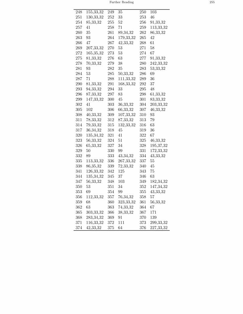
Further Reading 255
248 155,33,32 249 35 250 103251 130,33,32 252 33 253 46254 85,33,32 255 52 256 91,33,32257 41 258 71 259 113,33,32260 35 261 89,34,32 262 86,33,32263 93 264 179,33,32 265 42266 47 267 42,33,32 268 61269 207,33,32 270 53 271 58272 165,35,32 273 53 274 67275 81,33,32 276 63 277 91,33,32278 70,33,32 279 38 280 242,33,32281 93 282 35 283 53,33,32284 53 285 50,33,32 286 69287 71 288 111,33,32 289 36290 81,33,32 291 168,33,32 292 37293 94,33,32 294 33 295 48296 87,33,32 297 83 298 61,33,32299 147,33,32 300 45 301 83,33,32302 41 303 36,33,32 304 203,33,32305 102 306 66,33,32 307 46,33,32308 40,33,32 309 107,33,32 310 93311 78,33,32 312 87,33,32 313 79314 79,33,32 315 132,33,32 316 63317 36,34,32 318 45 319 36320 135,34,32 321 41 322 67323 56,33,32 324 51 325 46,33,32326 65,33,32 327 34 328 195,37,32329 50 330 99 331 172,33,32332 89 333 43,34,32 334 43,33,32335 113,33,32 336 267,33,32 337 55338 86,35,32 339 72,33,32 340 45341 126,33,32 342 125 343 75344 135,34,32 345 37 346 63347 56,33,32 348 103 349 182,34,32350 53 351 34 352 147,34,32353 69 354 99 355 43,33,32356 112,33,32 357 76,34,32 358 57359 68 360 323,33,32 361 56,33,32362 63 363 74,33,32 364 67365 303,33,32 366 38,33,32 367 171368 283,34,32 369 91 370 139371 116,33,32 372 111 373 299,33,32374 42,33,32 375 64 376 227,33,32
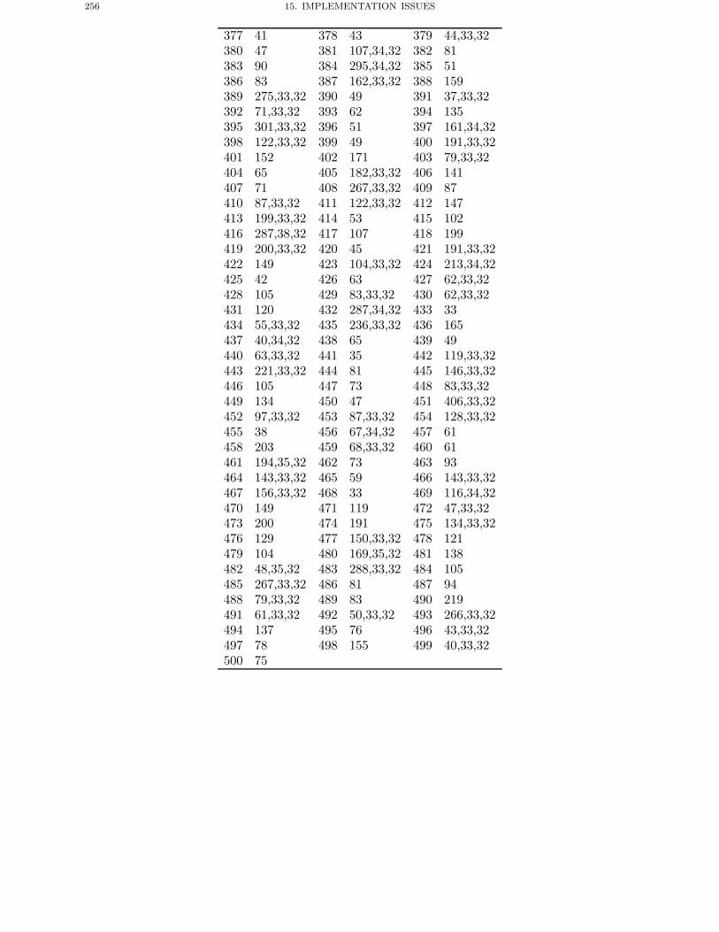
256 15. IMPLEMENTATION ISSUES
377 41 378 43 379 44,33,32380 47 381 107,34,32 382 81383 90 384 295,34,32 385 51386 83 387 162,33,32 388 159389 275,33,32 390 49 391 37,33,32392 71,33,32 393 62 394 135395 301,33,32 396 51 397 161,34,32398 122,33,32 399 49 400 191,33,32401 152 402 171 403 79,33,32404 65 405 182,33,32 406 141407 71 408 267,33,32 409 87410 87,33,32 411 122,33,32 412 147413 199,33,32 414 53 415 102416 287,38,32 417 107 418 199419 200,33,32 420 45 421 191,33,32422 149 423 104,33,32 424 213,34,32425 42 426 63 427 62,33,32428 105 429 83,33,32 430 62,33,32431 120 432 287,34,32 433 33434 55,33,32 435 236,33,32 436 165437 40,34,32 438 65 439 49440 63,33,32 441 35 442 119,33,32443 221,33,32 444 81 445 146,33,32446 105 447 73 448 83,33,32449 134 450 47 451 406,33,32452 97,33,32 453 87,33,32 454 128,33,32455 38 456 67,34,32 457 61458 203 459 68,33,32 460 61461 194,35,32 462 73 463 93464 143,33,32 465 59 466 143,33,32467 156,33,32 468 33 469 116,34,32470 149 471 119 472 47,33,32473 200 474 191 475 134,33,32476 129 477 150,33,32 478 121479 104 480 169,35,32 481 138482 48,35,32 483 288,33,32 484 105485 267,33,32 486 81 487 94488 79,33,32 489 83 490 219491 61,33,32 492 50,33,32 493 266,33,32494 137 495 76 496 43,33,32497 78 498 155 499 40,33,32500 75
CHAPTER 16
Obtaining Authentic Public Keys
Chapter Goals
• To describe the notion of digital certificates.• To explain the notion of a PKI.• To examine different approaches such as X509, PGP and SPKI.• To show how an implicit certificate scheme can operate.• To explain how identity based cryptographic schemes operate.
1. Generalities on Digital Signatures
Digital signatures have a number of uses which go beyond the uses of handwritten signatures.For example we can use digital signatures to
• control access to data,• allow users to authenticate themselves to a system,• allow users to authenticate data,• sign ‘real’ documents.
Each application has a different type of data being bound, a different length of the lifetime of thedata to be signed, different types of principals performing the signing and verifying and differentawareness of the data being bound.
For example an interbank payment need only contain the two account numbers and the amount.It needs to be signed by the payee and verified only by the computer which will carry out thetransfer. The lifetime of the signature is only until the accounts are reconciled, for example whenthe account statements are sent to the customers and a suitable period has elapsed to allow thecustomers to complain of any error.
As another example consider a challenge response authentication mechanism. Here the user,to authenticate itself to the device, signs a challenge provided by the device. The lifetime of thesignature may only be a few seconds. The user of course assumes that the challenge is random andis not a hash of an interbank payment. Hence, it is probably prudent that we use different keys forour authentication tokens and our banking applications.
As a final example consider a digital will or a mortgage contract. The length of time that thissignature must remain valid may (hopefully in the case of a will) be many years. Hence, the securityrequirements for long-term legal documents will be very different from those of an authenticationtoken.
You need to remember however that digital signatures are unlike handwritten signatures in thatthey are
• NOT necessarily on a document: Any piece of digital stuff can be signed.• NOT transferable to other documents: Unlike a handwritten signature, a digital signature
is different on each document.
257
258 16. OBTAINING AUTHENTIC PUBLIC KEYS
• NOT modifiable after they are made: One cannot alter the document and still have thedigital signature remaining valid.
• NOT produced by a person: A digital signature is never produced by a person, unless thesignature scheme is very simple (and weak) or the person is a mathematical genius.
All they do is bind knowledge of an unrevealed private key to a particular piece of data.
2. Digital Certificates and PKI
When using a symmetric key system we assume we do not have to worry about which key belongsto which principle. It is tacitly assumed, see for example the chapter dealing with symmetric keyagreement protocols and the BAN logic, that if Alice holds a long-term secret key Kab which shethinks is shared with Bob, then Bob really does have a copy of the same key. This assurance is oftenachieved using a trusted physical means of long-term key distribution, using for example armedcouriers.
In a public key system the issues are different. Alice may have a public key which she thinks isassociated with Bob, but we usually do not assume that Alice is 100 percent certain that it reallybelongs to Bob. This is because we do not, in the public key model, assume a physically secure keydistribution system. After all, that was the point of public key cryptography in the first place: tomake key management easier. Alice may have obtained the public key she thinks belongs to Bobfrom Bob’s web page, but how does she know the web page has not been spoofed?
The process of linking a public key to an entity or principal, be it a person, machine or process,is called binding. One way of binding, common in many applications where the principal really doesneed to be present, is by using a physical token such as a smart card. Possession of the token, andknowledge of any PIN/password needed to unlock the token, is assumed to be equivalent to beingthe designated entity. This solution has a number of problems associated with it, since cards canbe lost or stolen, which is why we protect them using a PIN (or in more important applications byusing biometrics). The major problem is that most entities are non-human, they are computers andcomputers do not carry cards. In addition many public key protocols are performed over networkswhere physical presence of the principal (if it is human) is not something one can test.
Hence, some form of binding is needed which can be used in a variety of very different applica-tions. The main binding tool in use today is the digital certificate. In this a special trusted thirdparty, or TTP, called a certificate authority, or CA, is used to vouch for the validity of the publickeys.
A CA based system works as follows:• All users have a trusted copy of the public key of the CA. For example these come embedded
in your browser when you buy your computer, and you ‘of course’ trust the vendor of thecomputer and the manufacturer of the software on your computer.
• The CA’s job is to digitally sign data strings containing the following information(Alice, Alice’s public key).
This data string, and the associated signature is called a digital certificate. The CA willonly sign this data if it truly believes that the public key really does belong to Alice.
• When Alice now sends you her public key, contained in a digital certificate, you now trustthat the purported key really is that of Alice, since you trust the CA to do its job correctly.
This use of a digital certificate binds the name ‘Alice’ with the ‘Key’, it is therefore often calledan identity certificate. Other bindings are possible, we shall see some of these later related toauthorizations.
Public key certificates will typically (although not always) be stored in repositories and accessedas required. For example, most browsers keep a list of the certificates that they have come across.The digital certificates do not need to be stored securely since they cannot be tampered with asthey are digitally signed.
2. DIGITAL CERTIFICATES AND PKI 259
To see the advantage of certificates and CAs in more detail consider the following example of aworld without a CA. In the following discussion we break with our colour convention for a momentand now use red to signal public keys which must be obtained in an authentic manner and blue tosignal public keys which do not need to be obtained in an authentic manner.
In a world without a CA you obtain many individual public keys from each individual in someauthentic fashion. For example
6A5DEF....A21 Jim Bean’s public key,7F341A....BFF Jane Doe’s public key,B5F34A....E6D Microsoft’s update key.
Hence, each key needs to be obtained in an authentic manner, as does every new key you obtain.Now consider the world with a CA. You obtain a single public key in an authentic manner,
namely the CA’s public key. We shall call our CA Ted since he is trustworthy. You then obtainmany individual public keys, signed by the CA, in possibly an unauthentic manner. For examplethey could be attached at the bottom of an email, or picked up whilst browsing the web.
A45EFB....C45 Ted’s totally trustworthy key,6A5DEF....A21 Ted says ‘This is Jim Bean’s public key’,7F341A....BFF Ted says ‘This is Jane Doe’s public key’,B5F34A....E6D Ted says ‘This is Microsoft’s update key’.
If you trust Ted’s key and you trust Ted to do his job correctly then you trust all the public keysyou hold to be authentic.
In general a digital certificate is not just a signature on the single pair
(Alice, Alice’s public key),one can place all sorts of other, possibly application specific, information into the certificate. Forexample it is usual for the certificate to contain the following information.
• user’s name,• user’s public key,• is this an encryption or signing key?• name of the CA,• serial number of the certificate,• expiry date of the certificate,• . . . .
Commercial certificate authorities exist who will produce a digital certificate for your public key,often after payment of a fee and some checks on whether you are who you say you are. Thecertificates produced by commercial CAs are often made public, so one can call them public ‘publickey certificates’, in that there use is mainly over open public networks.
CAs are also used in proprietary systems, for example in debit/credit card systems or by largecorporations. In such situations it may be the case that the end users do not want their publickey certificates to be made public, in which case one can call them private ‘public key certificates’.But one should bear in mind that whether the digital certificate is public or private should noteffect the security of the private key associated to the public key contained in the certificate. Thedecision to make one’s certificates private is often one of business rather than security.
It is common for more than one CA to exist. A quick examination of the properties of yourweb browser will reveal a large number of certificate authorities which your browser assumes you‘trust’ to perform the function of a CA. As there are more than one CA it is common for one CA tosign a digital certificate containing the public key of another CA, and vice versa, a process whichis known as cross-certification.
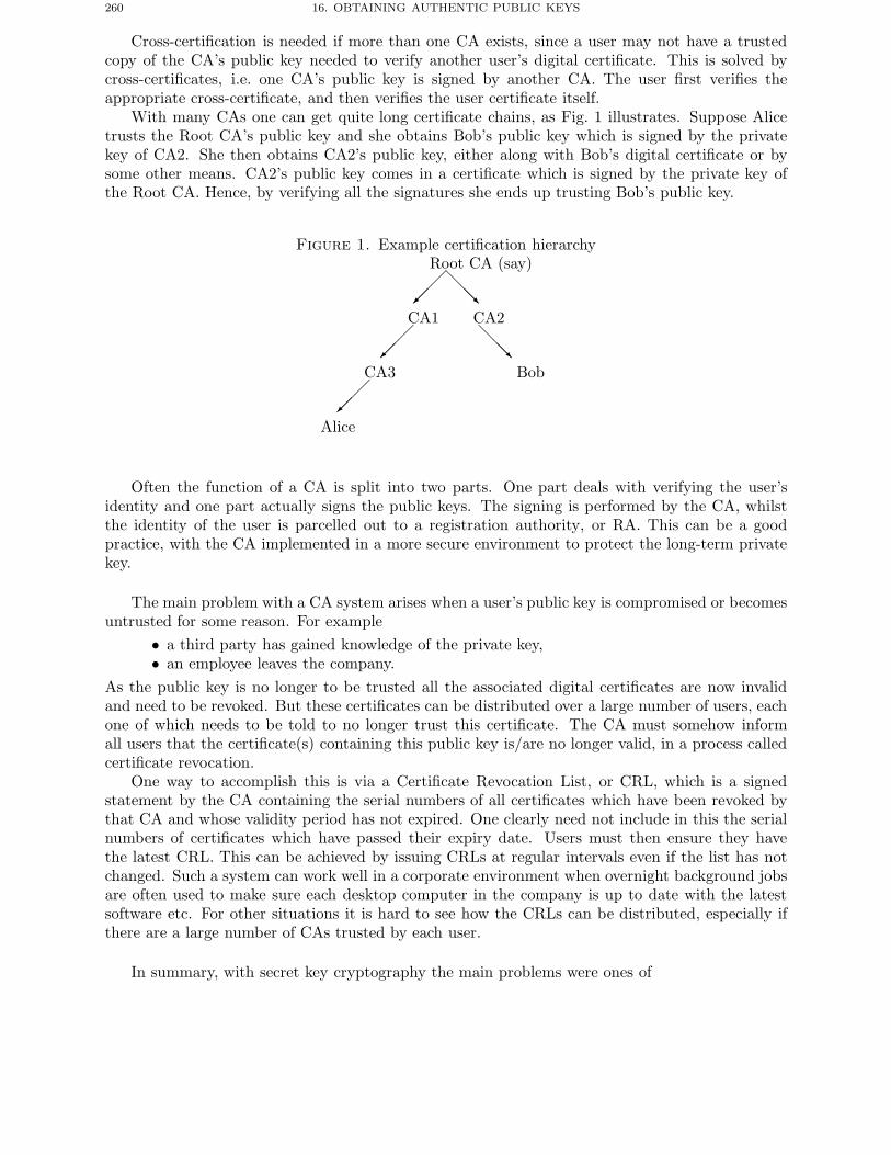
260 16. OBTAINING AUTHENTIC PUBLIC KEYS
Cross-certification is needed if more than one CA exists, since a user may not have a trustedcopy of the CA’s public key needed to verify another user’s digital certificate. This is solved bycross-certificates, i.e. one CA’s public key is signed by another CA. The user first verifies theappropriate cross-certificate, and then verifies the user certificate itself.
With many CAs one can get quite long certificate chains, as Fig. 1 illustrates. Suppose Alicetrusts the Root CA’s public key and she obtains Bob’s public key which is signed by the privatekey of CA2. She then obtains CA2’s public key, either along with Bob’s digital certificate or bysome other means. CA2’s public key comes in a certificate which is signed by the private key ofthe Root CA. Hence, by verifying all the signatures she ends up trusting Bob’s public key.
Figure 1. Example certification hierarchyRoot CA (say)
�
����
CA1�
���
CA2
�CA3
����
Bob
Alice
Often the function of a CA is split into two parts. One part deals with verifying the user’sidentity and one part actually signs the public keys. The signing is performed by the CA, whilstthe identity of the user is parcelled out to a registration authority, or RA. This can be a goodpractice, with the CA implemented in a more secure environment to protect the long-term privatekey.
The main problem with a CA system arises when a user’s public key is compromised or becomesuntrusted for some reason. For example
• a third party has gained knowledge of the private key,• an employee leaves the company.
As the public key is no longer to be trusted all the associated digital certificates are now invalidand need to be revoked. But these certificates can be distributed over a large number of users, eachone of which needs to be told to no longer trust this certificate. The CA must somehow informall users that the certificate(s) containing this public key is/are no longer valid, in a process calledcertificate revocation.
One way to accomplish this is via a Certificate Revocation List, or CRL, which is a signedstatement by the CA containing the serial numbers of all certificates which have been revoked bythat CA and whose validity period has not expired. One clearly need not include in this the serialnumbers of certificates which have passed their expiry date. Users must then ensure they havethe latest CRL. This can be achieved by issuing CRLs at regular intervals even if the list has notchanged. Such a system can work well in a corporate environment when overnight background jobsare often used to make sure each desktop computer in the company is up to date with the latestsoftware etc. For other situations it is hard to see how the CRLs can be distributed, especially ifthere are a large number of CAs trusted by each user.
In summary, with secret key cryptography the main problems were ones of
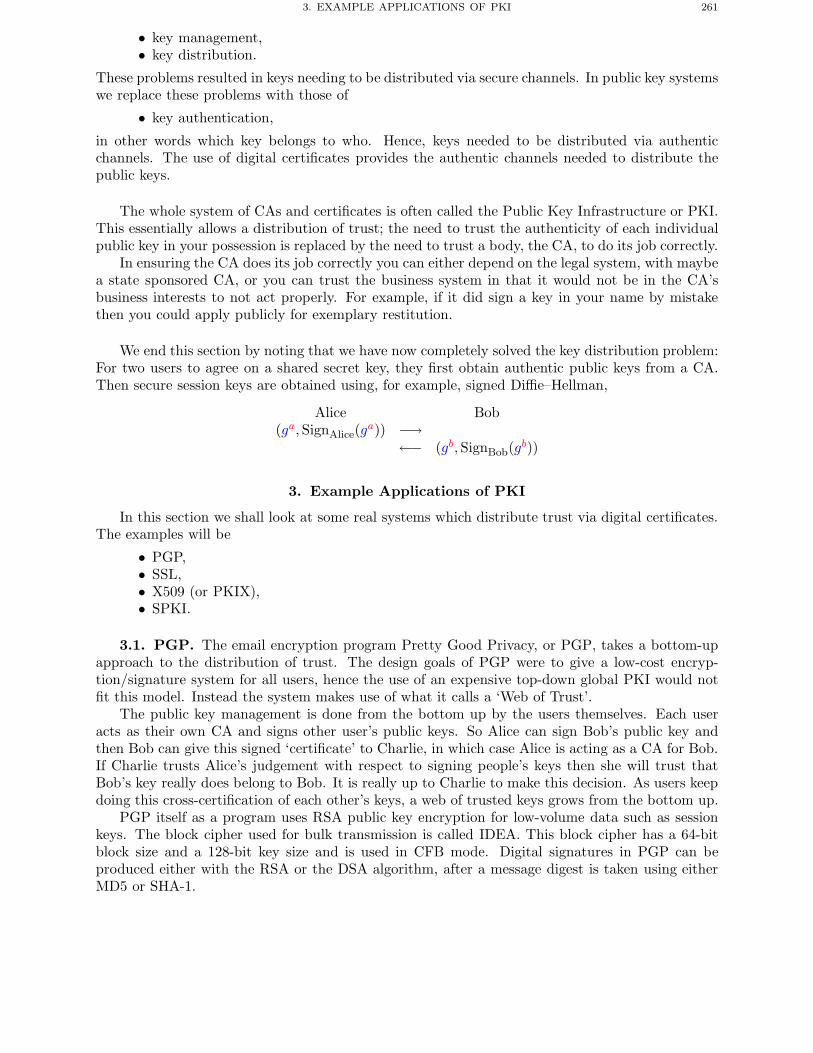
3. EXAMPLE APPLICATIONS OF PKI 261
• key management,• key distribution.
These problems resulted in keys needing to be distributed via secure channels. In public key systemswe replace these problems with those of
• key authentication,
in other words which key belongs to who. Hence, keys needed to be distributed via authenticchannels. The use of digital certificates provides the authentic channels needed to distribute thepublic keys.
The whole system of CAs and certificates is often called the Public Key Infrastructure or PKI.This essentially allows a distribution of trust; the need to trust the authenticity of each individualpublic key in your possession is replaced by the need to trust a body, the CA, to do its job correctly.
In ensuring the CA does its job correctly you can either depend on the legal system, with maybea state sponsored CA, or you can trust the business system in that it would not be in the CA’sbusiness interests to not act properly. For example, if it did sign a key in your name by mistakethen you could apply publicly for exemplary restitution.
We end this section by noting that we have now completely solved the key distribution problem:For two users to agree on a shared secret key, they first obtain authentic public keys from a CA.Then secure session keys are obtained using, for example, signed Diffie–Hellman,
Alice Bob(ga,SignAlice(ga)) −→
←− (gb,SignBob(gb))
3. Example Applications of PKI
In this section we shall look at some real systems which distribute trust via digital certificates.The examples will be
• PGP,• SSL,• X509 (or PKIX),• SPKI.
3.1. PGP. The email encryption program Pretty Good Privacy, or PGP, takes a bottom-upapproach to the distribution of trust. The design goals of PGP were to give a low-cost encryp-tion/signature system for all users, hence the use of an expensive top-down global PKI would notfit this model. Instead the system makes use of what it calls a ‘Web of Trust’.
The public key management is done from the bottom up by the users themselves. Each useracts as their own CA and signs other user’s public keys. So Alice can sign Bob’s public key andthen Bob can give this signed ‘certificate’ to Charlie, in which case Alice is acting as a CA for Bob.If Charlie trusts Alice’s judgement with respect to signing people’s keys then she will trust thatBob’s key really does belong to Bob. It is really up to Charlie to make this decision. As users keepdoing this cross-certification of each other’s keys, a web of trusted keys grows from the bottom up.
PGP itself as a program uses RSA public key encryption for low-volume data such as sessionkeys. The block cipher used for bulk transmission is called IDEA. This block cipher has a 64-bitblock size and a 128-bit key size and is used in CFB mode. Digital signatures in PGP can beproduced either with the RSA or the DSA algorithm, after a message digest is taken using eitherMD5 or SHA-1.
262 16. OBTAINING AUTHENTIC PUBLIC KEYS
The keys that an individual trusts are held in a so-called key ring. This means users havecontrol over their own local public key store. This does not rule out a centralized public key store,but means one is not necessarily needed.
Key revocation is still a problem with PGP as with all such systems. The ad-hoc methodadopted by PGP is that if your key is compromised then you should tell all your friends, who havea copy of your key, to delete the key from their key ring. All your friends should then tell all theirfriends and so on.
3.2. Secure Socket Layer. Whilst the design of PGP was driven by altruistic ideals, namelyto provide encryption for the masses, the Secure Socket Layer, or SSL, was driven by commercialrequirements, namely to provide a secure means for web based shopping and sales. Essentially SSLadds security to the TCP level of the IP stack. It provides security of data and not parties butallows various protocols to be transparently layered on top, for example HTTP, FTP, TELNET,etc.
The primary objective was to provide channel security, to enable the encrypted transmission ofcredit card details or passwords. After an initial handshake all subsequent traffic is encrypted. Theserver side of the communication, namely the website or the host computer in a Telnet session, isalways authenticated for the benefit of the client. Optionally the client may be authenticated tothe user, but this is rarely done in practice for web based transactions.
As in PGP, bulk encryption is performed using a block or stream cipher (usually either DESor an algorithm from the RC family). The choice of precise cipher is chosen between the client andserver during the initial handshake. The session key to be used is derived using standard protocolssuch as the Diffie–Hellman protocol, or RSA based key transport.
The server is authenticated since it provides the client with an X509 public key certificate. This,for web shopping transactions, is signed by some global CA whose public key comes embedded intothe user’s web browser. For secure Telnet sessions (often named SSH after the program which runsthem) the server side certificate is usually a self-signed certificate from the host computer.
The following is a simplified overview of how SSL can operate.• The client establishes connection with the server on a special port number so as to signal
this will be a secure session.• The server sends a certified public key to the client.• The client verifies the certificate and decides whether it trusts this public key.• The client chooses a random secret.• The client encodes this with the server’s public key and sends this back to the server.• The client and server now securely share the secret.• The server now authenticates itself to the client by responding using the shared secret.
The determination of session keys can be a costly operation for both the server and the client,especially when the data may come in bursts, as when one is engaged in shopping transactions, orperforming some remote access to a computer. Hence, there is some optimization made to enablereuse of session keys. The client is allowed to quote a previous session key, the server can eitheraccept it or ask for a new one to be created. So as to avoid any problems this ability is limitedby two rules. Firstly a session key should have a very limited lifetime and secondly any fatal errorin any part of the protocols will immediately invalidate the session key and require a new one tobe determined. In SSL the initial handshake is also used for the client and the server to agree onwhich bulk encryption algorithm to use, this is usually chosen from the list of RC4, RC5, DES orTriple DES.
3.3. X509 Certificates. When discussing SSL we mentioned that the server uses an X509public key certificate. X509 is a standard which defines a structure for public key certificates,currently it is the most widely deployed certificate standard. A CA assigns a unique name to each
3. EXAMPLE APPLICATIONS OF PKI 263
user and issues a signed certificate. The name is often the URL or email address. This can causeproblems since, for example, many users may have different versions of the same email address. Ifyou send a signed email containing your certificate for your email ‘address’
[email protected] your email program sends this from the ‘address’
[email protected], even though you consider both addresses to be equivalent, the email client of the recipientwill often complain saying that the signature is not to be trusted.
The CAs are connected in a tree structure, with each CA issuing a digital certificate for the onebeneath it. In addition cross-certification between the branches is allowed. The X509 certificatesthemselves are defined in standards using a language called ASN.1, or Abstract Syntax Notation.This can be rather complicated at first sight and the processing of all the possible options oftenends up with incredible ‘code bloat’.
The basic X509 certificate structure is very simple, but can end up being very complex in anyreasonable application. This is because some advanced applications may want to add additionalinformation into the certificates which enable authorization and other capabilities. However, thefollowing records are always in a certificate.
• The version number of the X509 standard which this certificate conforms to.• The certificate serial number.• The CA’s signing algorithm identifier. This should specify the algorithm and the domain
parameters used, if the CA has multiple possible algorithms or domain parameters.• The issuer’s name, i.e. the name of the issuing CA.• The validity period in the form of a not-before and not-after date.• The subject’s name, i.e. whose public key is being signed. This could be an email address
or a domain name.• The subject’s public key. This contains the algorithm name and any associated domain
parameters plus the actual value of the public key• The issuer’s signature on the subject’s public key and all data that is to be bound to the
subject’s public key, such as the subject’s name.
3.4. SPKI. In response to some of the problems associated with X509, another type of certifi-cate format has been proposed called SPKI, or Simple Public Key Infrastructure. This system aimsto bind authorizations as well as identities, and also tries to deal with the issue of delegation ofauthorizations and trust. Thus it may be suitable for business to business e-commerce transactions.For example, when managers go on holiday they can delegate their authorizations for certain tasksto their subordinates.
SPKI does not assume the global CA hierarchy which X509 does. It assumes a more ground-upapproach like PGP. However, it is currently not used much commercially since PKI vendors havea lot of investment in X509 and are probably not willing to switch over to a new system (and thedesktop applications such as your web browser would also need significant alterations).
Instead of using ASN.1 to describe certificates, SPKI uses S-expressions. These are LISP-likestructures which are very simple to use and describe. In addition S-expressions can be made verysimple even for humans to understand, as opposed to the machine-only readable formats of X509certificates. S-expressions can even come with display hints to enable greater readability. Thecurrent draft standard specifies these display hints as simple MIME-types.
Each SPKI certificate has an issuer and a subject both of which are public keys (or a hash ofa public key), and not names. This is because SPKI’s authors claim that it is a key which doessomething and not a name. After all it is a key which is used to sign a document etc. Focusingon the keys also means we can concentrate more on the functionality. There are two types of
264 16. OBTAINING AUTHENTIC PUBLIC KEYS
SPKI certificates: ones for binding identities to keys and ones for binding authorizations to keys.Internally these are represented as tuples of 4 and 5 objects, which we shall now explain.
3.4.1. SPKI 4-Tuples. To give an identity certificate and bind a name with a key, like X509does, SPKI uses a 4-tuple structure. This is an internal abstraction of what the certificate representsand is given by:
(Issuer, Name, Subject, Validity).In real life this would consist of the following five fields:
• issuer’s public key,• name of the subject,• subject’s public key,• validity period,• signature of the issuer on the triple (Name, Subject, Validity).
Anyone is able to issue such a certificate, and hence become a CA.3.4.2. SPKI 5-Tuples. 5-tuples are used to bind keys to authorizations. Again this is an internal
abstraction of what the certificate represents and is given by(Issuer, Subject, Delegation, Authorization, Validity).
In real life this would consist of the following six fields:• issuer’s public key.• subject’s public key.• delegation. A ‘Yes’ or ‘No’ flag, saying whether the subject can delegate the permission
or not.• authorization. What the subject is being given permission to do• validity. How long the authorization is for.• signature of the issuer on the quadruple (S,D,A,V).
One can combine an authorization certificate and an identity certificate to obtain an audit trail.This is needed since the authorization certificate only allows a key to perform an action. It doesnot say who owns the key. To find out who owns a key you need to use an identity certificate.
When certificate chains are eventually checked to enable some authorization, a 5-tuple reductionprocedure is carried out. This can be represented by the following rule
(I1, S1,D1, A1, V1) + (I2, S2,D2, A2, V2)
= (I1, S2,D2, A1 ∩A2, V1 ∩ V2).
This equality holds only if• S1 = I2• D1 = true.
This means the first two certificates together can be interpreted as the third. This third 5-tuple isnot really a certificate, it is the meaning of the first two when they are presented together.
As an example we will show how combining two 5-tuples is equivalent to delegating authority.Suppose our first 5-tuple is given by:
• I1 = Alice• S1 = Bob• D1 = true• A1 = Spend up to £100 on Alice’s account• V1 = forever.
So Alice allows Bob to spend up to £100 on her account and allows Bob to delegate this authorityto anyone he chooses.
Now consider the second 5-tuple given by
4. OTHER APPLICATIONS OF TRUSTED THIRD PARTIES 265
• I2 = Bob• S2 = Charlie• D2 = false• A2 = Spend between £50 and £200 on Alice’s account• V2 = before tomorrow morning.
So Bob is saying Charlie can spend between £50 and £200 of Alice’s money, as long as it happensbefore tomorrow morning.
We combine these two 5-tuples, using the 5-tuple reduction rule, to form the new 5-tuple• I3 = Alice• S3 = Charlie• D3 = false• A3 = Spend between £50 and £100 on Alice’s account• V3 = before tomorrow morning.
Since Alice has allowed Bob to delegate she has in effect allowed Charlie to spend between £50 and£100 on her account before tomorrow morning.
4. Other Applications of Trusted Third Parties
In some applications it is necessary for signatures to remain valid for a long time. Revocationof a public key, even long after the legitimate creation of the signature, potentially invalidates alldigital signatures made using that key, even those in the past. This is a major problem if digitalsignatures are to be used for documents of long-term value such as wills, life insurance and mortgagecontracts. We essentially need methods to prove that a digital signature was made prior to therevocation of the key and not after it. This brings us to the concept of time stamping.
A time stamping service is a means whereby a trusted entity will take a signed message, adda date/timestamp and sign the result using its own private key. This proves when a signature wasmade (like a notary service in standard life insurance). However, there is the requirement that thepublic key of the time stamping service must never be revoked. An alternative to the use of a timestamping service is the use of a secure archive for signed messages.
As another application of a trusted third-party consider the problem associated with keepingtruly secret keys for encryption purposes.
• What if someone loses or forgets a key? They could lose all your encrypted data.• What if the holder of the key resigns from the company or is killed? The company may
now want access to the encrypted data.• What if the user is a criminal? Here the government may want access to the encrypted
data.One solution is to deposit a copy of your key with someone else in case you lose yours, or somethinguntoward happens. On the other hand, simply divulging the key to anybody, even the government,is very insecure.
A proposed solution is key escrow implemented via a secret sharing scheme. Here the privatekey is broken into pieces, each of which can be verified to be correct. Each piece is then given tosome authority. At some later point if the key needs to be recovered then a subset of the authoritiescan come together and reconstruct it from their shares. The authorities implementing this escrowfacility are another example of a Trusted Third Party, since you really have to trust them. Infact the trust required is so high that this solution has been a source of major debate within thecryptographic and governmental communities in the past. The splitting of the key between thevarious escrow authorities can be accomplished using the trick of a secret sharing scheme which wewill discuss in Chapter 23.
266 16. OBTAINING AUTHENTIC PUBLIC KEYS
5. Implicit Certificates
One issue with digital certificates is that they can be rather large. Each certificate needs to atleast contain both the public key of the user and the signature of the certificate authority on thatkey. This can lead to quite large certificate sizes, as the following table demonstrates:
RSA DSA EC-DSAUser’s key 1024 1024 160CA sig 1024 320 320
This assumes for RSA keys one uses a 1024-bit modulus, for DSA one uses a 1024-bit prime pand a 160-bit prime q and for EC-DSA one uses a 160-bit curve. Hence, for example, if the CA isusing 1024-bit RSA and they are signing the public key of a user using 1024-bit DSA then the totalcertificate size must be at least 2048 bits. An interesting question is whether this can be madesmaller.
Implicit certificates enable this. An implicit certificate looks like
X|Ywhere
• X is the data being bound to the public key,• Y is the implicit certificate on X.
From Y we need to be able to recover the public key being bound to X and implicit assurance thatthe certificate was issued by the CA. In the system we describe below, based on a DSA or EC-DSA,the size of Y will be 1024 or 160 bits respectively. Hence, the size of the certificate is reduced tothe size of the public key being certified.
5.1. System Setup. The CA chooses a public group G of known order n and an elementP ∈ G. The CA then chooses a long-term private key c and computes the public key
Q = P c.
This public key should be known to all users.
5.2. Certificate Request. Suppose Alice wishes to request a certificate and the public keyassociated to the information ID, which could be her name. Alice computes an ephemeral secretkey t and an ephemeral public key
R = P t.
Alice sends R and ID to the CA.
5.3. Processing of the request. The CA checks that he wants to link ID with Alice. TheCA picks another random number k and computes
g = P kR = P kP t = P k+t.
Then the CA computess = cH(ID‖g) + k (mod n).
Then the CA sends back to Alice the pair
(g, s).
The implicit certificate is the pair(ID, g).
We now have to convince you that• Alice can recover a valid public/private key pair,• any other user can recover Alice’s public key from this implicit certificate
6. IDENTITY BASED CRYPTOGRAPHY 267
5.4. Alice’s Key Discovery. Alice knows the following information
t, s,R = P t.
From this she can recover her private key
a = t+ s (mod n).
Note, Alice’s private key is known only to Alice and not to the CA. In addition Alice has contributedsome randomness t to her private key, as has the CA who contributed k. Her public key is then
P a = P t+s = P tP s = R · P s.
5.5. User’s Key Discovery. Since s and R are public, a user, say Bob, can recover Alice’spublic key from the above message flows via
R · P s.But this says nothing about the linkage between the CA, Alice’s public key and the ID information.Instead Bob recovers the public key from the implicit certificate
(ID, g)
and the CA’s public keyQ
via the equationP a = QH(ID‖g)g.
As soon as Bob sees Alice’s key used in action, say he verifies a signature purported to have beenmade by Alice, he knows implicitly that it must have been issued by the CA, since otherwise Alice’ssignature would not verify correctly.
There are a number of problems with the above system which mean that implicit certificatesare not used much in real life. For example,
(1) What do you do if the CA’s key is compromised? Usually you pick a new CA key andre-certify the user’s keys. But you cannot do this since the user’s public key is choseninteractively during the certification process.
(2) Implicit certificates require the CA and users to work at the same security level. This isnot considered good practice, as usually one expects the CA to work at a higher securitylevel (say 2048-bit DSA) than the user (say 1024-bit DSA).
However for devices with restricted bandwidth they can offer a suitable alternative where traditionalcertificates are not available.
6. Identity Based Cryptography
Another way of providing authentic public keys, without the need for certificates, is to use asystem whereby the user’s key is given by their identity. Such a system is called an identity basedencryption scheme or an identity based signature scheme. Such systems do not remove the needfor a trusted third-party to perform the original authentication of the user, but they do howeverremove the need for storage and transmission of certificates.
The first scheme of this type was a signature scheme invented by Shamir in 1984. It was notuntil 2001 however that an identity based encryption scheme was given by Boneh and Franklin.We shall only describe the original identity based signature scheme of Shamir, which is based onthe RSA problem.
268 16. OBTAINING AUTHENTIC PUBLIC KEYS
A trusted third-party first calculates an RSA modulus N , keeping the two factors secret. TheTTP also publishes a public exponent e, keeping the corresponding private exponent d to them-selves. In addition there is decided a mapping
I : {0, 1}∗ −→ (Z/NZ)∗
which takes bit strings to elements of (Z/NZ)∗. Such a mapping could be implemented by a hashfunction.
Now suppose Alice wishes to obtain the private key g corresponding to her name ‘Alice’. Thisis calculated for her by the TTP using the equation
g = I(Alice)d (mod N).
To sign a message m, Alice generates the pair (t, s) via the equations
t = re (mod N),
s = g · rH(m‖t) (mod N),
where r is a random integer and H is a hash function.To verify the signature (t, s) on the message m another user can do this, simply by knowing the
TTP’s public data and the identity of Alice, by checking that the following equation holds moduloN ,
I(Alice) · tH(m‖t) = ge · re·H(m‖t)
=(g · rH(m‖t)
)e= se.
Chapter Summary
• Digital certificates allow us to bind a public key to some other information, such as anidentity.
• This binding of key with identity allows us to solve the problem of how to distributeauthentic public keys.
• Various PKI systems have been proposed, all of which have problems and benefits associ-ated with them.
• PGP and SPKI work from the bottom up, whilst X509 works in a top-down manner.• SPKI contains the ability to delegate authorizations from one key to another.• Other types of trusted third-party applications exist such as time stamping and key escrow.• Implicit certificates aim to reduce the bandwidth requirements of standard certificates,
however they come with a number of drawbacks.• Identity based cryptography helps authenticate a user’s public key by using their identity
as the public key, but it does not remove the need for trusted third parties.
Further Reading

Further Reading 269
A good overview of the issues related to PKI can be found in the book by Adams and Lloyd.For further information on PGP and SSL look at the books by Garfinkel and Rescorla.
C. Adams and S. Lloyd. Understanding Public-Key Infrastructure: Concepts, Standards and De-ployment Considerations. New Riders Publishing, 1999.
S. Garfinkel. PGP: Pretty Good Privacy. O’Reilly & Associates, 1994.
E. Rescorla. SSL and TLS: Design and Building Secure Systems. Addison-Wesley, 2000.

Part 4
Security Issues
Having developed the basic public key cryptographic primitives we require, we now show thatthis is not enough. Often weaknesses occur because the designers of a primitive do not envisagehow the primitive is actually going to be used in real life. We first outline a number of attacks, andthen we try and define what it means to be secure; this leads us to deduce that the primitives wehave given earlier are not really secure enough.
This then leads us to look at two approaches to build secure systems. One based on purecomplexity theory ends up being doomed to failure, since pure complexity theory is about worstcase rather than average case hardness of problems. The second approach of provable security endsup being more suitable and has in fact turned out to be highly influential on modern cryptography.This second approach also derives from complexity theory, but is based on the relative average casehardness of problems, rather than the absolute hardness of the worst case instance.

CHAPTER 17
Attacks on Public Key Schemes
Chapter Goals
• To explain Wiener’s attack based on continued fractions.• To describe lattice basis reduction algorithms and give some examples of how they are
used to break cryptographic systems.• To explain the technique of Coppersmith for finding small roots of modular polynomial
equations and describe some of the cryptographic applications.• To introduce the notions of partial key exposure and fault analysis.
1. Introduction
In this chapter we explain a number of attacks against naive implementations of schemes suchas RSA and DSA. We shall pay particular attention to the techniques of Coppersmith, based onlattice basis reduction. What this chapter aims to do is show you that even though a cryptographicprimitive such as the RSA function
x −→ xe (mod N)
is a trapdoor one-way permutation, this on its own is not enough to build secure encryption systems.It all depends on how you use the RSA function. In later chapters we go on to show how one canbuild secure systems out of the RSA function and the other public key primitives we have met.
2. Wiener’s Attack on RSA
We have mentioned in earlier chapters that often one uses a small public RSA exponent e soas to speed up the public key operations in RSA. Sometimes we have applications where it is moreimportant to have a fast private key operation. Hence, one could be tempted to choose a smallvalue of the private exponent d. Clearly this will lead to a large value of the encryption exponent eand we cannot choose too small a value for d, otherwise an attacker could find d using exhaustivesearch. However, it turns out that d needs to be at least the size of 1
3N1/4 due to an ingenious
attack by Wiener which uses continued fractions.
Let α ∈ R, we define the following sequences, starting with α0 = α, p0 = a0 and q0 = 1,p1 = a0a1 + 1 and q1 = a1,
ai = �αi�,αi+1 =
1αi − ai
,
pi = aipi−1 + pi−2 for i ≥ 2,qi = aiqi−1 + qi−2 for i ≥ 2.
273
274 17. ATTACKS ON PUBLIC KEY SCHEMES
The integers a0, a1, a2, . . . are called the continued fraction expansion of α and the fractionspiqi
are called the convergents. The denominators of these convergents grow at an exponential rate andthe convergent above is a fraction in its lowest terms since one can show
gcd(pi, qi) = 1
for all values of i.The important result is that if p and q are two integers with∣∣∣∣α− p
q
∣∣∣∣ ≤ 12q2
then pq is a convergent in the continued fraction expansion of α.
Wiener’s attack uses continued fractions as follows. We assume we have an RSA modulusN = pq with q < p < 2q. In addition assume that the attacker knows that we have a smalldecryption exponent d < 1
3N1/4. The encryption exponent e is given to the attacker, where this
exponent satisfiesed = 1 (mod Φ),
withΦ = φ(N ) = (p − 1)(q − 1).
We also assume e < Φ, since this holds in most systems. First notice that this means there is aninteger k such that
ed− kΦ = 1.
Hence, we have ∣∣∣∣ eΦ − k
d
∣∣∣∣ = 1dΦ
.
Now, Φ ≈ N , since|N − Φ| = |p+ q − 1| < 3
√N.
So we should have that eN is a close approximation to k
d .∣∣∣∣ eN − k
d
∣∣∣∣ =∣∣∣∣ed−Nk
dN
∣∣∣∣=∣∣∣∣ed− kΦ −Nk + kΦ
dN
∣∣∣∣=∣∣∣∣1 − k(N − Φ))
dN
∣∣∣∣≤∣∣∣∣∣3k
√N
dN
∣∣∣∣∣=
3kd√N.
Since e < Φ, it is clear that we have k < d, which is itself less than 13N
1/4 by assumption. Hence,∣∣∣∣ eN − k
d
∣∣∣∣ < 12d2
.
3. LATTICES AND LATTICE REDUCTION 275
Since gcd(k, d) = 1 we see that kd will be a fraction in its lowest terms. Hence, the fraction
k
dmust arise as one of the convergents of the continued fraction expansion of
e
N.
The correct one can be detected by simply testing which one gives a d which satisfies
(me)d = m (mod N)
for some random value of m. The total number of convergents we will need to take is of orderO(logN), hence the above gives a linear time algorithm to determine the private exponent whenit is less than 1
3N1/4.
As an example suppose we have the RSA modulus
N = 9449 868 410 449
with the public keye = 6792 605 526 025.
We are told that the decryption exponent satisfies d < 13N
1/4 ≈ 584. To apply Wiener’s attack wecompute the continued fraction expansion of the number
α =e
N,
and check each denominator of a convergent to see whether it is equal to the private key d. Theconvergents of the continued fraction expansion of α are given by
1,23,34,57,1825,2332,409569
,16592308
, . . .
Checking each denominator in turn we see that the decryption exponent is given by
d = 569,
which is the denominator of the 7th convergent.
3. Lattices and Lattice Reduction
We shall see later in this chapter that lattice basis reduction provides a crucial tool in variousattacks on a number of public key systems. So we spend this section giving an overview of thisimportant area. We first need to recap on some basic linear algebra.
Suppose x = (x1, x2, . . . , xn) is an n-dimension real vector, i.e. for all i we have xi ∈ R. Theset of all such vectors is denoted Rn. On two such vectors we can define an inner product
〈x, y〉 = x1y1 + x2y2 + · · · + xnyn,
which is a function from pairs of n-dimensional vectors to the real numbers. You probably learntat school that two vectors x and y are orthogonal, or meet at right angles, if and only if we have
〈x, y〉 = 0.
Given the inner product we can then define the size, or length, of a vector by
‖x‖ =√
〈x, x〉 =√x2
1 + x22 + · · · + x2
n.
This length corresponds to the intuitive notion of length of vectors which we have, in particularthe length satisfies a number of properties.
• ‖x‖ ≥ 0, with equality if and only if x is the zero vector.
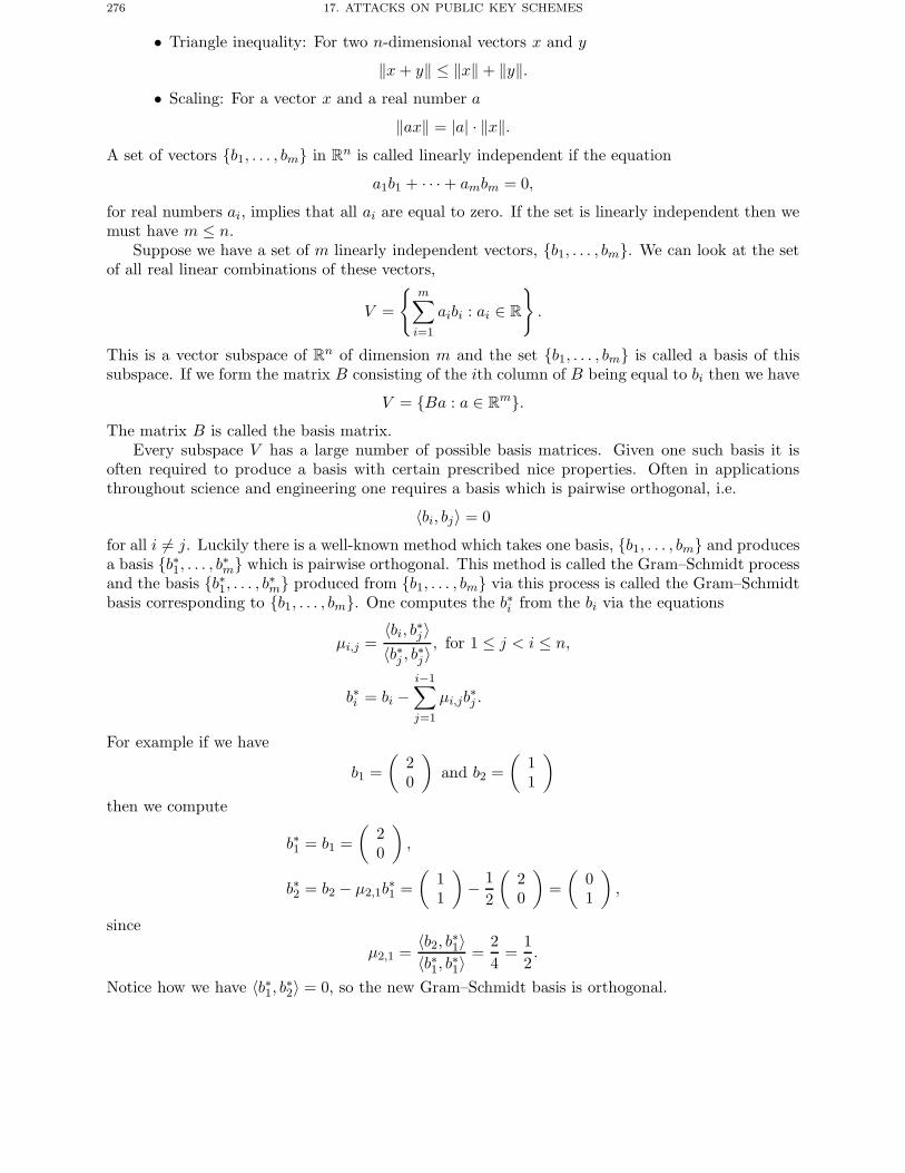
276 17. ATTACKS ON PUBLIC KEY SCHEMES
• Triangle inequality: For two n-dimensional vectors x and y
‖x+ y‖ ≤ ‖x‖ + ‖y‖.• Scaling: For a vector x and a real number a
‖ax‖ = |a| · ‖x‖.A set of vectors {b1, . . . , bm} in Rn is called linearly independent if the equation
a1b1 + · · · + ambm = 0,
for real numbers ai, implies that all ai are equal to zero. If the set is linearly independent then wemust have m ≤ n.
Suppose we have a set of m linearly independent vectors, {b1, . . . , bm}. We can look at the setof all real linear combinations of these vectors,
V =
{m∑i=1
aibi : ai ∈ R
}.
This is a vector subspace of Rn of dimension m and the set {b1, . . . , bm} is called a basis of thissubspace. If we form the matrix B consisting of the ith column of B being equal to bi then we have
V = {Ba : a ∈ Rm}.The matrix B is called the basis matrix.
Every subspace V has a large number of possible basis matrices. Given one such basis it isoften required to produce a basis with certain prescribed nice properties. Often in applicationsthroughout science and engineering one requires a basis which is pairwise orthogonal, i.e.
〈bi, bj〉 = 0
for all i �= j. Luckily there is a well-known method which takes one basis, {b1, . . . , bm} and producesa basis {b∗1, . . . , b∗m} which is pairwise orthogonal. This method is called the Gram–Schmidt processand the basis {b∗1, . . . , b∗m} produced from {b1, . . . , bm} via this process is called the Gram–Schmidtbasis corresponding to {b1, . . . , bm}. One computes the b∗i from the bi via the equations
μi,j =〈bi, b∗j 〉〈b∗j , b∗j〉
, for 1 ≤ j < i ≤ n,
b∗i = bi −i−1∑j=1
μi,jb∗j .
For example if we have
b1 =(
20
)and b2 =
(11
)then we compute
b∗1 = b1 =(
20
),
b∗2 = b2 − μ2,1b∗1 =(
11
)− 1
2
(20
)=(
01
),
since
μ2,1 =〈b2, b∗1〉〈b∗1, b∗1〉
=24
=12.
Notice how we have 〈b∗1, b∗2〉 = 0, so the new Gram–Schmidt basis is orthogonal.
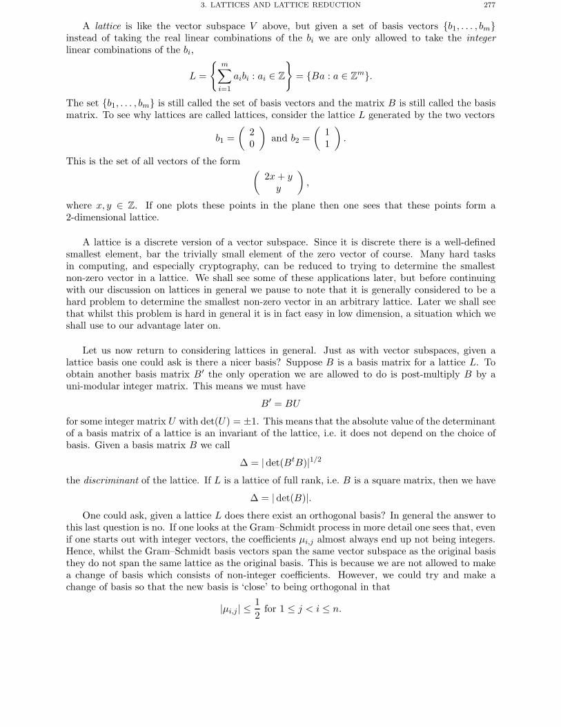
3. LATTICES AND LATTICE REDUCTION 277
A lattice is like the vector subspace V above, but given a set of basis vectors {b1, . . . , bm}instead of taking the real linear combinations of the bi we are only allowed to take the integerlinear combinations of the bi,
L =
{m∑i=1
aibi : ai ∈ Z
}= {Ba : a ∈ Zm}.
The set {b1, . . . , bm} is still called the set of basis vectors and the matrix B is still called the basismatrix. To see why lattices are called lattices, consider the lattice L generated by the two vectors
b1 =(
20
)and b2 =
(11
).
This is the set of all vectors of the form (2x+ yy
),
where x, y ∈ Z. If one plots these points in the plane then one sees that these points form a2-dimensional lattice.
A lattice is a discrete version of a vector subspace. Since it is discrete there is a well-definedsmallest element, bar the trivially small element of the zero vector of course. Many hard tasksin computing, and especially cryptography, can be reduced to trying to determine the smallestnon-zero vector in a lattice. We shall see some of these applications later, but before continuingwith our discussion on lattices in general we pause to note that it is generally considered to be ahard problem to determine the smallest non-zero vector in an arbitrary lattice. Later we shall seethat whilst this problem is hard in general it is in fact easy in low dimension, a situation which weshall use to our advantage later on.
Let us now return to considering lattices in general. Just as with vector subspaces, given alattice basis one could ask is there a nicer basis? Suppose B is a basis matrix for a lattice L. Toobtain another basis matrix B′ the only operation we are allowed to do is post-multiply B by auni-modular integer matrix. This means we must have
B′ = BU
for some integer matrix U with det(U) = ±1. This means that the absolute value of the determinantof a basis matrix of a lattice is an invariant of the lattice, i.e. it does not depend on the choice ofbasis. Given a basis matrix B we call
Δ = |det(BtB)|1/2
the discriminant of the lattice. If L is a lattice of full rank, i.e. B is a square matrix, then we have
Δ = |det(B)|.One could ask, given a lattice L does there exist an orthogonal basis? In general the answer to
this last question is no. If one looks at the Gram–Schmidt process in more detail one sees that, evenif one starts out with integer vectors, the coefficients μi,j almost always end up not being integers.Hence, whilst the Gram–Schmidt basis vectors span the same vector subspace as the original basisthey do not span the same lattice as the original basis. This is because we are not allowed to makea change of basis which consists of non-integer coefficients. However, we could try and make achange of basis so that the new basis is ‘close’ to being orthogonal in that
|μi,j| ≤ 12
for 1 ≤ j < i ≤ n.
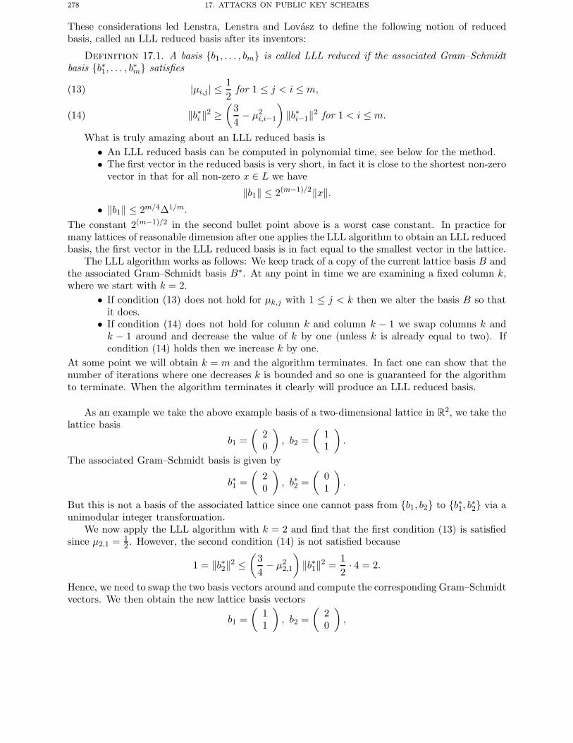
278 17. ATTACKS ON PUBLIC KEY SCHEMES
These considerations led Lenstra, Lenstra and Lovasz to define the following notion of reducedbasis, called an LLL reduced basis after its inventors:
Definition 17.1. A basis {b1, . . . , bm} is called LLL reduced if the associated Gram–Schmidtbasis {b∗1, . . . , b∗m} satisfies
|μi,j | ≤ 12
for 1 ≤ j < i ≤ m,(13)
‖b∗i ‖2 ≥(
34− μ2
i,i−1
)‖b∗i−1‖2 for 1 < i ≤ m.(14)
What is truly amazing about an LLL reduced basis is• An LLL reduced basis can be computed in polynomial time, see below for the method.• The first vector in the reduced basis is very short, in fact it is close to the shortest non-zero
vector in that for all non-zero x ∈ L we have
‖b1‖ ≤ 2(m−1)/2‖x‖.• ‖b1‖ ≤ 2m/4Δ1/m.
The constant 2(m−1)/2 in the second bullet point above is a worst case constant. In practice formany lattices of reasonable dimension after one applies the LLL algorithm to obtain an LLL reducedbasis, the first vector in the LLL reduced basis is in fact equal to the smallest vector in the lattice.
The LLL algorithm works as follows: We keep track of a copy of the current lattice basis B andthe associated Gram–Schmidt basis B∗. At any point in time we are examining a fixed column k,where we start with k = 2.
• If condition (13) does not hold for μk,j with 1 ≤ j < k then we alter the basis B so thatit does.
• If condition (14) does not hold for column k and column k − 1 we swap columns k andk − 1 around and decrease the value of k by one (unless k is already equal to two). Ifcondition (14) holds then we increase k by one.
At some point we will obtain k = m and the algorithm terminates. In fact one can show that thenumber of iterations where one decreases k is bounded and so one is guaranteed for the algorithmto terminate. When the algorithm terminates it clearly will produce an LLL reduced basis.
As an example we take the above example basis of a two-dimensional lattice in R2, we take thelattice basis
b1 =(
20
), b2 =
(11
).
The associated Gram–Schmidt basis is given by
b∗1 =(
20
), b∗2 =
(01
).
But this is not a basis of the associated lattice since one cannot pass from {b1, b2} to {b∗1, b∗2} via aunimodular integer transformation.
We now apply the LLL algorithm with k = 2 and find that the first condition (13) is satisfiedsince μ2,1 = 1
2 . However, the second condition (14) is not satisfied because
1 = ‖b∗2‖2 ≤(
34− μ2
2,1
)‖b∗1‖2 =
12· 4 = 2.
Hence, we need to swap the two basis vectors around and compute the corresponding Gram–Schmidtvectors. We then obtain the new lattice basis vectors
b1 =(
11
), b2 =
(20
),
4. LATTICE BASED ATTACKS ON RSA 279
with the associated Gram–Schmidt basis vectors
b∗1 =(
11
), b∗2 =
(1
−1
).
We now go back to the first condition again. This time we see that we have μ2,1 = 1 which violatesthe first condition. To correct this we subtract one lot of b1 from the vector b2 so as to obtainμ2,1 = 0. We now find the lattice basis is given by
b1 =(
11
), b2 =
(1
−1
)and the Gram–Schmidt basis is then identical to this lattice basis, in that
b∗1 =(
11
), b∗2 =
(1
−1
).
Now we are left to check the second condition again, we find
2 = ‖b∗2‖2 ≥(
34− μ2
2,1
)‖b∗1‖2 =
34· 2 =
32.
Hence, both conditions are satisfied and we conclude that
b1 =(
11
), b2 =
(1
−1
)is a reduced basis for the lattice L.
We end this introduction to lattices by noticing that there is a link between continued fractionsand lattice reduction. Applying the continued fraction algorithm to a real number α is used to findvalues of p and q, with q not too large, so that
|qα− p|is small. A similar effect can be achieved using lattices by applying the LLL algorithm to the latticegenerated by the columns of the matrix (
1 0Cα −C
),
for some constant C. This is because the lattice L contains the ‘short’ vector(q
C(qα− p)
)=(
1 0Cα −C
)·(qp
).
In some sense we therefore can consider the LLL algorithm to be a multi-dimensional generalizationof the continued fraction algorithm.
4. Lattice Based Attacks on RSA
In this section we examine how lattices can be used to attack certain systems, when some otherside information is known. This is analogous to Wiener’s attack above where one could breakRSA given the side information that the decryption exponent was exceedingly short. Much ofthe work in this area is derived from initial work of Coppersmith, which was later simplified byHowgrave-Graham.
The basic technique is a method to solve the following problem: Given a polynomial
f(x) = f0 + f1x+ · · · + fd−1xd−1 + xd
over the integers of degree d and the side information that there exists a root x0 modulo N whichis small, say |x0| < N1/d, can one efficiently find the small root x0? The answer is surprisingly yes,and this leads to a number of interesting cryptographic consequences.
280 17. ATTACKS ON PUBLIC KEY SCHEMES
The basic idea is to find a polynomial h(x) ∈ Z[x] which has the same root modulo N as thetarget polynomial f(x) does. This new polynomial h(x) should be small in the sense that the normof its coefficients,
‖h‖2 =deg(h)∑i=0
h2i
should be small. If such an h(x) can be found then we can appeal to the following lemma.
Lemma 17.2. Let h(x) ∈ Z[x] denote a polynomial of degree at most n and let X and N bepositive integers. Suppose
‖h(xX)‖ < N/√n
then if |x0| < X satisfiesh(x0) = 0 (mod N)
then h(x0) = 0 over the integers and not just modulo N .
Now we return to our original polynomial f(x) of degree d and notice that if
f(x0) = 0 (mod N)
then we also havef(x0)k = 0 (mod Nk).
Moreover, if we set, for some given value of m,
gu,v(x) = Nm−vxuf(x)v
thengu,v(x0) = 0 (mod Nm)
for all 0 ≤ u < d and 0 ≤ v ≤ m. We then fix m and try to find au,v ∈ Z so that
h(x) =∑u≥0
m∑v=0
au,vgu,v(x)
satisfies the conditions of the above lemma.In other words we wish to find integer values of au,v so that the resulting polynomial h satisfies
‖h(xX)‖ ≤ Nm/√d(m+ 1),
with
h(xX) =∑u≥0
m∑v=0
au,vgu,v(xX).
This is a minimization problem which can be solved using lattice basis reduction, as we shall nowshow in a simple example.
Suppose our polynomial f(x) is given by
f(x) = x2 + ax+ b
and we wish to find an x0 such that
f(x0) = 0 (mod N).
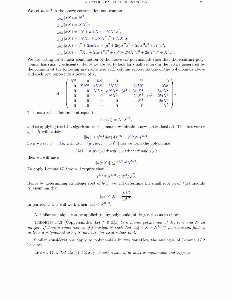
4. LATTICE BASED ATTACKS ON RSA 281
We set m = 2 in the above construction and compute
g0,0(xX) = N2,
g1,0(xX) = XN 2x,
g0,1(xX) = bN + aXNx+NX2x2,
g1,1(xX) = bNXx+ aNX2x2 +NX3x3,
g0,2(xX) = b2 + 2baXx+ (a2 + 2b)X2x2 + 2aX3x3 +X4x4,
g1,2(xX) = b2Xx+ 2baX2x2 + (a2 + 2b)X3x3 + 2aX4x4 +X5x5.
We are asking for a linear combination of the above six polynomials such that the resulting poly-nomial has small coefficients. Hence we are led to look for small vectors in the lattice generated bythe columns of the following matrix, where each column represents one of the polynomials aboveand each row represents a power of x,
A =
⎛⎜⎜⎜⎜⎜⎜⎝
N2 0 bN 0 b2 00 XN2 aXN bNX 2abX Xb2
0 0 NX2 aNX2 (a2 + 2b)X2 2abX2
0 0 0 NX3 2aX3 (a2 + 2b)X3
0 0 0 0 X4 2aX4
0 0 0 0 0 X5
⎞⎟⎟⎟⎟⎟⎟⎠.
This matrix has determinant equal to
det(A) = N6X15,
and so applying the LLL algorithm to this matrix we obtain a new lattice basis B. The first vectorb1 in B will satisfy
‖b1‖ ≤ 26/4 det(A)1/6 = 23/2NX5/2.
So if we set b1 = Au, with Bu = (u1, u2, . . . , u6)t, then we form the polynomial
h(x) = u1g0,0(x) + u2g1,0(x) + · · · + u6g1,2(x)
then we will have‖h(xX)‖ ≤ 23/2NX5/2.
To apply Lemma 17.2 we will require that
23/2NX5/2 < N2/√
6.
Hence by determining an integer root of h(x) we will determine the small root x0 of f(x) moduloN assuming that
|x0| ≤ X =N2/5
481/5.
In particular this will work when |x0| ≤ N0.39.
A similar technique can be applied to any polynomial of degree d so as to obtain
Theorem 17.3 (Coppersmith). Let f ∈ Z[x] be a monic polynomial of degree d and N aninteger. If there is some root x0 of f modulo N such that |x0| ≤ X = N1/d−ε then one can find x0
in time a polynomial in logN and 1/ε, for fixed values of d.
Similar considerations apply to polynomials in two variables, the analogue of Lemma 17.2becomes:
Lemma 17.4. Let h(x, y) ∈ Z[x, y] denote a sum of at most w monomials and suppose
282 17. ATTACKS ON PUBLIC KEY SCHEMES
• h(x0, y0) = 0 (mod N e) for some positive integers N and e where the integers x0 and y0
satisfy |x0| < X and |y0| < Y ,• ‖h(xX, yY )‖ < N e/
√w.
Then h(x0, y0) = 0 holds over the integers.
However, the analogue of Theorem 17.3 then becomes only a heuristic result.We now use Theorem 17.3 and its generalizations to describe a number of attacks against RSA.
4.1. Hastad’s Attack. In Chapter 11 we saw the following attack on the RSA system: Giventhree public keys (Ni, ei) all with the same encryption exponent ei = 3, if a user sent the samemessage to all three public keys then an adversary could recover the plaintext using the ChineseRemainder Theorem.
Now suppose that we protect against this attack by insisting that before encrypting a messagem we first pad with some user-specific data. For example the ciphertext becomes, for user i,
ci = (i · 2h +m)3 (mod Ni).
However, one can still break this system using an attack due to Hastad. Hastad’s attack is relatedto Coppersmith’s Theorem since we can interpret the attack scenario, generalized to k users andpublic encryption exponent e, as being given k polynomials of degree e
gi(x) = (i · 2h + x)e − ci, 1 ≤ i ≤ k.
Then given that there is an m such that
gi(m) = 0 (mod Ni),
the goal is to recover m. We can assume that m is smaller than any one of the moduli Ni. Setting
N = N1N2 · · ·Nk
and using the Chinese Remainder Theorem we can find ti so that
g(x) =k∑i=1
tigi(x)
andg(m) = 0 (mod N).
Then, since g has degree e and is monic, using Theorem 17.3 we can recover m in polynomial time,as long as we have at least as many ciphertexts as the encryption exponent i.e. k > e, since
m < miniNi < N1/k < N1/e.
4.2. Franklin–Reiter Attack and Coppersmith’s Generalization. Now suppose we haveone RSA public key (N, e) owned by Alice. The Franklin–Reiter attack applies to the followingsituation: Bob wishes to send two related messages m1 and m2 to Alice, where the relation is givenby the public polynomial
m1 = f(m2) (mod N).Given c1 and c2 an attacker has a good chance of determining m1 and m2 for any small encryptionexponent e. The attack is particularly simple when
f = ax+ b and e = 3,
with a and b fixed and given to the attacker. The attacker knows that m2 is a root, modulo N , ofthe two polynomials
g1(x) = x3 − c2,
g2(x) = f(x)3 − c1.
4. LATTICE BASED ATTACKS ON RSA 283
So the linear factor x−m2 divides both g1(x) and g2(x).We now form the greatest common divisor of g1(x) and g2(x). Strictly speaking this is not
possible in general since Z/NZ[x] is not a Euclidean ring, but if the Euclidean algorithm breaksdown then we would find a factor of N and so be able to find Alice’s private key in any case. Onecan show that when
f = ax+ b and e = 3,
the resulting gcd, when it exists, must always be the linear factor x−m2, and so the attacker canalways find m2 and then m1.
Coppersmith extended the attack of Franklin and Reiter, in a way which also extends thepadding result from Hastad’s attack. Suppose before sending a message m we pad it with somerandom data. So for example if N is an n-bit RSA modulus and m is a k-bit message then wecould append n− k random bits to either the top or bottom of the message. Say
m′ = 2n−km+ r
where r is some, per message, random number of length n − k. Coppersmith showed that thispadding is insecure.
Suppose Bob sends the same message to Alice twice, i.e. we have ciphertexts c1 and c2 corre-sponding to the messages
m1 = 2n−km+ r1,
m2 = 2n−km+ r2,
where r1, r2 are two different random (n − k)-bit numbers. The attacker sets y0 = r2 − r1 and isled to solve the simultaneous equations
g1(x, y) = xe − c1,
g2(x, y) = (x+ y)e − c2.
The attacker forms the resultant h(y) of g1(x, y) and g2(x, y) with respect to x. Now y0 = r2 − r1is a small root of the polynomial h(y), which has degree e2. Using Coppersmith’s Theorem 17.3the attacker recovers r2 − r1 and then recovers m2 using the method of the Franklin–Reiter attack.
Whilst the above trivial padding scheme is therefore insecure, one can find secure paddingschemes for the RSA encryption algorithm. We shall return to padding schemes for RSA in Chap-ter 20.
4.3. Extension to Wiener’s Attack. Recall that Wiener’s attack on RSA applied when itwas known that the private decryption exponent d was small, in the sense that
d ≤ 13N1/4.
Boneh and Durfee, using an analogue of the bivariate case of Coppersmith’s Theorem 17.3, extendedWiener’s attack to the case where
d ≤ N0.292,
using a heuristic algorithm. We do not go into the details but show how Boneh and Durfee proceedto a problem known as the small inverse problem.
Suppose we have an RSA modulus N , with encryption exponent e and decryption exponent d.By definition there is an integer k such that
ed+kΦ2
= 1,
284 17. ATTACKS ON PUBLIC KEY SCHEMES
where Φ = φ(N). Expanding the definition of Φ we find
ed+ k
(N + 1
2− p+ q
2
)= 1.
We set
s = −p+ q
2,
A =N + 1
2.
Then finding d, where d is small say d < N δ, is equivalent to finding the two small solutions k ands to the following congruence
f(k, s) = k(A+ s) = 1 (mod e).
To see that k and s are small relative to the modulus e for the above equation, notice that e ≈ Nsince d is small, and so
|s| < 2N 0.5 ≈ e0.5 and |k| < 2deΦ
≤ 3deN
≈ eδ.
We can interpret this problem as finding an integer which is close to A whose inverse is smallmodulo e. This is called the small inverse problem. Boneh and Durfee show that this problem hasa solution when δ ≤ 0.292, hence extending the result of Wiener’s attack. This is done by applyingthe multivariate analogue of Coppersmith’s method to the polynomial f(k, s).
5. Partial Key Exposure Attacks
Partial key exposure is related to the following question: Suppose in some cryptographic schemethe attacker recovers a certain set of bits of the private key, can the attacker use this to recover thewhole private key? In other words, does partial exposure of the key result in a total break of thesystem? We shall present a number of RSA examples, however these are not the only ones. Thereare a number of results related to partial key exposure which relate to other schemes such as DSAor symmetric key based systems.
5.1. Partial Exposure of the MSBs of the RSA Decryption Exponent. Somewhatsurprisingly for RSA, in the more common case of using a small public exponent e, one can triviallyrecover half of the bits of the private key d, namely the most significant, as follows. Recall there isa value of k such that 0 < k < e with
ed− k(N − (p+ q) + 1) = 1.
Now suppose for each possible value of i, 0 < i ≤ e, the attacker computes
di = �(iN + 1)/e�.Then we have
|dk − d| ≤ k(p+ q)/e ≤ 3k√N/e < 3
√N.
Hence, dk is a good approximation for the actual value of d.Now when e = e it is clear that k, so we must have k = 2 and so d2 reveals half of the most
significant bits of d. Unluckily for the attack, and luckily for the user, there is no known way torecover the rest of d given only the most significant bits.
6. FAULT ANALYSIS 285
5.2. Partial Exposure of some bits of the RSA Prime Factors. Suppose our n-bit RSAmodulus N is given by p · q, with p ≈ q and that the attacker has found the n/4 least significantbits of p. Recall that p is only around n/2-bits long in any case, so this means the attacker is giventhe lower half of all the bits making up p. We write
p = x02n/4 + p0.
We then have, writing q = y02n/4 + q0,
N = p0q0 (mod 2n/4).
Hence, we can determine the value of q0. We now write down the polynomial
p(x, y) = (p0 + 2n/4x)(q0 + 2n/4y)
= p0q0 + 2n/4(p0y + q0x) + 2n/2xy.
Now p(x, y) is a bivariate polynomial of degree two which has known small solution modulo N ,namely (x0, y0) where 0 < x0, y0 ≤ 2n/4 ≈ N1/4. Hence, using the heuristic bivariate extensionof Coppersmith’s Theorem 17.3, we can recover x0 and y0 in polynomial time and so factor themodulo N .
A similar attack applies when the attacker knows the n/4 most significant bits of p.
5.3. Partial Exposure of the LSBs of the RSA Decryption Exponent. We now supposewe are given, for small public exponent e, a quarter of the least significant bits of the privateexponent d. That is we have d0 where
d = d0 + 2n/4x0
where 0 ≤ x0 ≤ 23n/4. Recall there is an even value of k with 0 < k < e such that
ed− k(N − (p+ q) + 1) = 1.
We then have, since N = pq,edp− kp(N − p+ 1) + kN = p.
If we set p0 = p (mod 2n/4) then we have the equation
(15) ed0p0 − kp0(N − p0 + 1) + kN − p0 = 0 (mod 2n/4).
This gives us the following algorithm to recover the whole of d. For each value of k less than ewe solve Equation (15) modulo 2n/4 for p0. Each value of k will result in O(n4 ) possible valuesfor p0. Using each of these values of p0 in turn, we apply the previous technique for factoring Nfrom Section 5.2. One such value of p0 will be the correct value of p (mod 2n/4) and so the abovefactorization algorithm will work and we can recover the value of d.
6. Fault Analysis
An interesting class of attacks results from trying to induce faults within a cryptographic system.We shall describe this area in relation to the RSA signature algorithm but similar attacks can bemounted on other cryptographic algorithms, both public and secret key.
Imagine we have a hardware implementation of RSA, in a smart card say. On input of somemessage m the chip will sign the message for us, using some internal RSA private key. The attackerwishes to determine the private key hidden within the smart card. To do this the attacker can try tomake the card perform some of the calculation incorrectly, by either altering the card’s environmentby heating or cooling it or by damaging the circuitry of the card in some way.
An interesting case is when the card uses the Chinese Remainder Theorem to perform thesigning operation, to increase efficiency, as explained in Chapter 15. The card first computes thehash of the message
h = H(m).
286 17. ATTACKS ON PUBLIC KEY SCHEMES
Then the card computes
sp = hdp (mod p),
sq = hdq (mod q),
where dp = d (mod p − 1) and dq = d (mod q − 1). The final signature is produced by the cardfrom sp and sq via the Chinese Remainder Theorem using
• u = (sq − sp)T (mod q),• s = sp + up,
where T = p−1 (mod q).Now suppose that the attacker can introduce a fault into the computation so that sp is computed
incorrectly. The attacker will then obtain a value of s such that
se �= h (mod p),
se = h (mod q).
Hence, by computingq = gcd(se − h,N)
we can factor the modulus.
Chapter Summary
• Using a small private decryption exponent in RSA is not a good idea due to Wiener’sattack.
• Lattices are discrete analogues of vector spaces, as such they have a shortest non-zerovector.
• Lattice basis reduction often allows us to find the shortest non-zero vector in a givenlattice.
• Coppersmith’s Theorem allows us to solve a modular polynomial equation when the so-lution is known to be small. The method works by building a lattice depending on thepolynomial and then applying lattice basis reduction to obtain short vectors within thislattice.
• The Hastad and Franklin–Reiter attacks imply that one needs to be careful when designingpadding schemes for RSA.
• Using Coppersmith’s Theorem one can show that the revealing of a proportion of the bitsof either p, q or d in RSA can lead to a complete break of the system.
Further Reading
The main paper on Coppersmith’s lattice based attacks on RSA is by Coppersmith himself.Coppersmith’s approach has itself been simplified somewhat in the paper of Howgrave-Graham.Our treatment of attacks on RSA in this chapter has closely followed the survey article by Boneh.A complete survey of lattice based methods in cryptography is given in the survey article by Nguyenand Stern.

Further Reading 287
D. Boneh. Twenty years of attacks on the RSA cryptosystem. Notices of the American Mathemat-ical Society (AMS), 46, 203–213, 1999.
D. Coppersmith. Small solutions to polynomial equations, and low exponent RSA vulnerabilities.J. Cryptology, 10, 233–260, 1997.
N. Howgrave-Graham. Finding small solutions of univariate modular equations revisited. In Cryp-tography and Coding, Springer-Verlag LNCS 1355, 131–142, 1997.
P. Nguyen and J. Stern. The two faces of lattices in cryptology. In CALC ’01, Springer-VerlagLNCS 2146, 146–180, 2001.

CHAPTER 18
Definitions of Security
Chapter Goals
• To explain the various notions of security of encryption schemes, especially semantic se-curity and indistinguishability of encryptions.
• To explain the various attack notions, in particular the adaptive chosen ciphertext attack.• To show how the concept of non-malleability and adaptive chosen ciphertext attacks are
related.• To examine the RSA and ElGamal encryption schemes in terms of these definitions of
security and attacks.• To explain notions related to the security of signature schemes.• To show that naive (unhashed) RSA signatures are not secure due to the homomorphic
property.
1. Security of Encryption
Up to now we have not looked much at how cryptographic primitives are turned into realprotocols and systems. In designing cryptographic systems we need to understand exactly whatsecurity properties are guaranteed by the primitives and how the schemes can be made secureagainst all possible attacks.
Essentially, a cryptographic primitive is something like the raw RSA function or the modularexponentiation operation. Both are one-way functions, the RSA function being a trap-door one-way function and modular exponentiation being a one-way function. One needs to be carefulhow one uses these primitives in a real scheme. For example the raw RSA function is completelydeterministic and so if used naively will always result in identical ciphertexts if you encrypt thesame plaintext twice under the same key. This is a bad idea as we saw in Chapters 11 and 17. Butthere is a more fundamental reason to avoid deterministic public key encryption algorithms; to seewhy you need to consider what it means for an encryption scheme to be secure.
There are three things we need to define• the goal of the adversary,• the types of attack allowed,• the computational model.
Our discussion will be in the context of public key encryption, but similar notions hold for symmetricciphers, see Chapter 21.
1.1. Notions of Security. There are essentially three notions of security which we need tounderstand,
• perfect security,• semantic security,• polynomial security.
289
290 18. DEFINITIONS OF SECURITY
We shall discuss each of these notions in turn. These notions are far stronger than the simplenotion of either recovering the private key or determining the plaintext which we have consideredpreviously.
1.1.1. Perfect Security: Recall that a scheme is said to have perfect security, or to have infor-mation theoretic security, if an adversary with infinite computing power can learn nothing aboutthe plaintext given the ciphertext. Shannon’s Theorem, Theorem 5.4, essentially states that thismeans that the key is as long as the message, and the same key is never used twice.
The problem is that such systems cannot exist in the public key model, since the encryptionkey is assumed to be used for many messages and is usually assumed to be very short.
1.1.2. Semantic Security: Semantic security is like perfect security but we only allow an ad-versary with polynomially bounded computing power. Formally, for all probability distributionson the message space whatever an adversary can compute in polynomial time about the plaintextgiven the ciphertext, they should also be able to compute without the ciphertext. In other words,having the ciphertext does not help finding anything about the message.
The following is a simplified formal definition: Suppose that the information we wish to computeon the message space is a single bit, i.e. there is some function
g : M −→ {0, 1}.We assume that over the whole message space we have
Pr (g(m) = 1) = Pr (g(m) = 0) =12,
and that the plaintexts and ciphertexts are all of the same length (so for example the length of theciphertext reveals nothing about the underlying plaintext).
The adversary we shall model as an algorithm S which on input of a public key y and a ciphertextc, encrypted under the public key y, will attempt to produce an evaluation of the function g on theplaintext for which c is the associated ciphertext. The output of S will therefore be a single bitcorresponding to the value of g.
The adversary is deemed to be successful if the probability of it being correct is greater thanone half. Clearly the adversary could always just guess the bit without seeing this ciphertext, hencewe are saying a successful adversary is one which can do better after seeing the ciphertext. Wetherefore define the advantage of the adversary S as
AdvS =∣∣∣∣Pr (S(c, y) = g(dx(c))) − 1
2
∣∣∣∣ ,where dx denotes decryption under the private key x associated to the public key y. A scheme isthen said to be semantically secure if we have
AdvS ≤ 1p(k)
,
for all adversaries S, all functions g and all polynomial functions p(k) when the security parameterk is sufficiently large.
1.1.3. Polynomial Security: The trouble with the definition of semantic security is that it ishard to show that a given encryption scheme has this property. Polynomial security, sometimescalled indistinguishability of encryptions, is a much easier property to show that a given systemhas. Luckily, we will show that if a system has polynomial security then it has semantic security.Hence, to show a system is semantically secure all we need do is show that it is polynomially secure.
A system is said to have indistinguishable encryptions, or to have polynomial security, if noadversary can win the following game with probability greater than one half. The adversary A isgiven a public key encryption function fy corresponding to some public key y. The adversary nowruns in two stages:
1. SECURITY OF ENCRYPTION 291
• Find: In the find stage the adversary produces two plaintext messages m0 and m1, ofequal length.
• Guess: The adversary is now given the encryption cb of one of the plaintexts mb forsome secret hidden bit b. The goal of the adversary is to now guess the value of b withprobability greater than one half.
Note, this means that an encryption function which is polynomially secure must be probabilistic innature, otherwise in the guess stage the adversary can compute
c1 = fy(m1)
and test whether this is equal to cb or not. The advantage of an adversary A is therefore definedto be
AdvA =∣∣∣∣Pr (A(guess, cb, y,m0,m1) = b) − 1
2
∣∣∣∣ ,since the adversary A could always simply guess the hidden bit b. A scheme is then said to bepolynomially secure if we have
AdvA ≤ 1p(k)
,
for all adversaries A and all polynomials p and sufficiently large k.
1.2. Notions of Attacks. At this stage we need to introduce various attack models. Thereare three basic attack models:
• passive attack, sometimes called a chosen plaintext attack, often denoted CPA,• chosen ciphertext attack, often denoted CCA1,• adaptive chosen ciphertext attack, often denoted CCA2.
1.2.1. Passive Attack: A passive attack is a very weak form of attack. The adversary Eve isallowed to look at various encrypted messages. She also has access to a (black) box which performsencryption but not decryption. Hence this models a simple attack on a public key system, since ina public key system everyone, including the attacker, has access to the encryption function.
1.2.2. Chosen Ciphertext Attack: A chosen ciphertext attack (CCA1) is often called a lunch-time attack and represents a slightly stronger form of attack. Eve is now given access to a black boxwhich performs decryptions. Eve can ask the box to decrypt a polynomial number of ciphertextsof her choosing, at lunch-time whilst the real user of the box is away at lunch. After this, at somepoint in the afternoon, she is given a target ciphertext and asked to decrypt this, or find informationabout the underlying plaintext, on her own, without using the box.
In the context of our game of polynomial security given above, this means that the adversarycan query the decryption box during the find stage of the algorithm but not the guess stage.
1.2.3. Adaptive Chosen Ciphertext Attack: An adaptive chosen ciphertext attack (CCA2) is avery strong form of attack. Eve is now allowed to ask the decryption box to decrypt any ciphertextof her choosing, bar the target ciphertext. It is widely regarded that any new proposed publickey encryption algorithm should meet the requirements of polynomial security under an adaptivechosen ciphertext attack.
Hence, in our game of polynomial security, the adversary can in both the find and guess stagesask the decryption box to decrypt any ciphertext, except they are not allowed to ask the box todecrypt the challenge cb, since otherwise the game would be far too easy.
The following definition is the accepted definition of what it means for a public encryptionscheme to be secure, a similar notion applies to symmetric key systems.
Definition 18.1. A public key encryption algorithm is said to be secure if it is semanticallysecure against an adaptive chosen ciphertext attack.
292 18. DEFINITIONS OF SECURITY
However, usually it is easier to show security under the following definition.
Definition 18.2. A public key encryption algorithm is said to be secure if it is polynomiallysecure against an adaptive chosen ciphertext attack.
These two notions are however related. For example, we shall now show the following importantresult:
Theorem 18.3. For a passive adversary, a system which is polynomially secure must necessarilybe semantically secure.
Proof. We proceed by contradiction. Assume that there is an encryption algorithm which isnot semantically secure, i.e. there is an algorithm S with
AdvS >1
p(k)
for a polynomial p(k) and all sufficiently large values of k. We shall show that it is then notpolynomial secure either. To do this we construct an adversary A against the polynomial securityof the scheme, which uses the adversary S against the semantic security as an oracle.
The find stage of adversary A outputs two messages m0 and m1 such that
g(m0) �= g(m1).
Such messages will be easy to find given our earlier simplified formal definition of semantic security,since the output of g is equiprobable over the whole message space.
The adversary A is then given an encryption cb of one of these and is asked to determine b. Inthe guess stage the adversary passes the ciphertext cb to the oracle S. The oracle S returns withits best guess as to the value of
g(mb).
The adversary A can now compare this value with that of g(m0) and g(m1) and hence output aguess as to what the value of b is.
Clearly if S is successful in breaking the semantic security of the scheme, then A will besuccessful in breaking the polynomial security. So
Pr (A(guess, cb, y,m0,m1) = b) = Pr (S(c, y) = g(dx(c))) .
So
AdvA = AdvS >1
p(k).
Hence, polynomial security must imply semantic security. �
Note, with a more complicated definition of semantic security it can be shown that for passiveadversaries the notions of semantic and polynomial security are equivalent.
1.3. Other Security Concepts.1.3.1. Non-Malleability: An encryption scheme is said to be non-malleable if given a ciphertext
C, corresponding to an unknown plaintext M , it is impossible to determine a valid ciphertext C ′ ona ‘related’ message M ′. Note, that ‘related’ is defined vaguely here on purpose. Non-malleability isimportant due to the following result, for which we only give an informal proof based on our vaguedefinition of non-malleability. A formal proof can however be given, with an associated formaldefinition of non-malleability.
Lemma 18.4. A malleable encryption scheme is not secure against an adaptive chosen ciphertextattack.
2. SECURITY OF ACTUAL ENCRYPTION ALGORITHMS 293
Proof. Suppose the scheme is malleable, then given the target ciphertext cb we alter it to arelated one, namely cb′. The relation should be such that there is also a known relationship betweenmb
′ and mb. Then the adversary can ask the decryption oracle to decrypt cb′ to reveal mb′, an
oracle query which is allowed in our prior game. Then from mb′ the adversary can recover mb. �
Later we shall show that almost all the public key schemes we have seen so far are malleable.However, it is known that a scheme which is non-malleable against a CCA2 attack is also polyno-mially secure against a CCA2 attack and viceversa. Hence, a non-malleable encryption scheme willmeet our previous definition of security of a public key encryption scheme.
1.3.2. Plaintext Aware: If a scheme is plaintext aware then we have a very strong notion ofsecurity. A scheme is called plaintext aware if it is computationally difficult to construct a validciphertext without being given the corresponding plaintext to start with. Hence, plaintext aware-ness implies one cannot mount a CCA attack. Since to write down a ciphertext requires you toknow the plaintext, so why would you ask the decryption oracle to decrypt the ciphertext?
Plaintext awareness has only been defined within the context of the random oracle model ofcomputation. In this model one assumes that idealized hash functions exist; these are one-wayfunctions which:
• take polynomial time to evaluate,• to an observer cannot be distinguished from random functions.
The random oracle model occurs in a number of proofs of security. These proofs tell us nothingabout the real-world security of the scheme under consideration. But they do show that any real-world attack must make use of the actual definition of the hash function deployed. The usual stateof affairs is that we prove a protocol secure in the random oracle model and then make a real-lifeprotocol by replacing the random oracle with a hash function like SHA-1 or MD5.
2. Security of Actual Encryption Algorithms
In this section we show that neither the RSA or ElGamal encryption algorithms meet ourstringent goals of semantic security against an adaptive chosen ciphertext attack. This shouldsurprise you since we have claimed that RSA is one of the most used and important algorithmsaround. But we have not shown you how RSA is actually used in practice. So far we have only giventhe simple mathematical description of the algorithms. As we progress onwards the mathematicsof public key encryption gets left behind and becomes replaced by cryptographic engineering.
To make the discussion easier we will use the fact that semantic security and indistinguishabilityof encryptions (polynomial security) are equivalent.
2.1. RSA.
Lemma 18.5. RSA is not polynomially secure.
Proof. Suppose the attacker knows that the user only encrypts one of two messages
m1 or m2.
These could be buy or sell, yes or no etc. The attacker is assumed to know the user’s publickey, namely N and e. On receiving the ciphertext c the attacker wants to determine whether thecorresponding plaintext m was equal to m1 or m2. All the adversary need do is compute
c′ = me1 (mod N).
Then• if c′ = c then the attacker knows that m = m1,• if c′ �= c then the attacker knows that m = m2.
�
294 18. DEFINITIONS OF SECURITY
The problem is that the attacker has access to the encryption function, it is a public key schemeafter all.
Now suppose that decryption was not injective, that each plaintext could correspond to a largenumber of ciphertexts. The exact ciphertext produced being determined by the encryption functionat runtime. In other words the encryption algorithm should be probabilistic in nature and not justdeterministic. Later we shall see a variant of RSA which has this property and so the attackdescribed in the above proof does not apply. But using a deterministic encryption function is notthe only problem with RSA.
Essentially RSA is malleable due to the homomorphic property.
Definition 18.6 (Homomorphic Property). Given the encryption of m1 and m2 we can deter-mine the encryption of m1 ·m2, without knowing m1 or m2.
That RSA has the homomorphic property follows from the equation
(m1 ·m2)e (mod N) = ((m1
e (mod N)) · (m2e (mod N))) (mod N).
One can use the homomorphic property to show that RSA is insecure under an adaptively chosenciphertext attack.
Lemma 18.7. RSA is not CCA2 secure.
Proof. Suppose the message Eve wants to break is
c = me (mod N).
Eve creates the ‘related’ ciphertext c′ = 2ec and asks her oracle to decrypt c′ to give m′. Eve canthen compute
m′
2=c′d
2=
(2ec)d
2
=2edcd
2=
2m2
= m.
�
2.2. ElGamal. Recall the decision Diffie–Hellman (known as DDH) assumption for a groupG = 〈g〉 is, given gx, gy and gz, determine whether
x · y = z (mod #G).
Lemma 18.8. If DDH is hard in the group G then ElGamal encryption is polynomially secureagainst a passive adversary.
Proof. To show that ElGamal encryption is polynomially secure assuming that DDH holdswe first assume that we have a polynomial-time algorithm A which breaks the polynomial securityof ElGamal encryption. Then using this algorithm A as a subroutine we give an algorithm to solvethe DDH problem. This is similar to the technique used in an earlier chapter where we showedthat an algorithm which could break ElGamal encryption, in the sense of decrypting a ciphertextto reveal a plaintext, could be used to solve the computational Diffie–Hellman problem. Now withour stronger definition of security, namely polynomial security, we can only relate breaking thesystem to the solution of a (supposedly) easier problem.
Recall A should run in two stages:• A find stage which outputs two messages and some state information and which takes a
public key as input.• A guess stage which takes as input a ciphertext, a public key, two messages and some
state information and guesses which plaintext the ciphertext corresponds to.
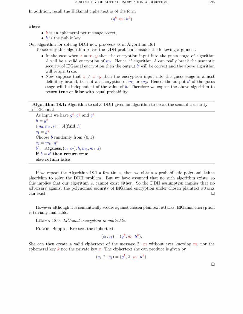
2. SECURITY OF ACTUAL ENCRYPTION ALGORITHMS 295
In addition, recall the ElGamal ciphertext is of the form
(gk,m · hk)where
• k is an ephemeral per message secret,• h is the public key.
Our algorithm for solving DDH now proceeds as in Algorithm 18.1To see why this algorithm solves the DDH problem consider the following argument.
• In the case when z = x · y then the encryption input into the guess stage of algorithmA will be a valid encryption of mb. Hence, if algorithm A can really break the semanticsecurity of ElGamal encryption then the output b′ will be correct and the above algorithmwill return true.
• Now suppose that z �= x · y then the encryption input into the guess stage is almostdefinitely invalid, i.e. not an encryption of m1 or m2. Hence, the output b′ of the guessstage will be independent of the value of b. Therefore we expect the above algorithm toreturn true or false with equal probability.
Algorithm 18.1: Algorithm to solve DDH given an algorithm to break the semantic securityof ElGamal
As input we have gx, gy and gz
h = gx
(m0,m1, s) = A(find, h)c1 = gy
Choose b randomly from {0, 1}c2 = mb · gzb′ = A(guess, (c1, c2), h,m0,m1, s)if b = b′ then return trueelse return false
If we repeat the Algorithm 18.1 a few times, then we obtain a probabilistic polynomial-timealgorithm to solve the DDH problem. But we have assumed that no such algorithm exists, sothis implies that our algorithm A cannot exist either. So the DDH assumption implies that noadversary against the polynomial security of ElGamal encryption under chosen plaintext attackscan exist. �
However although it is semantically secure against chosen plaintext attacks, ElGamal encryptionis trivially malleable.
Lemma 18.9. ElGamal encryption is malleable.
Proof. Suppose Eve sees the ciphertext
(c1, c2) = (gk,m · hk).She can then create a valid ciphertext of the message 2 · m without ever knowing m, nor theephemeral key k nor the private key x. The ciphertext she can produce is given by
(c1, 2 · c2) = (gk, 2 ·m · hk).�
296 18. DEFINITIONS OF SECURITY
One can use this malleability property, just as we did with RSA, to show that ElGamal encryp-tion is insecure under an adaptively chosen ciphertext attack.
Lemma 18.10. ElGamal is not CCA2 secure.
Proof. Suppose the message Eve wants to break is
c = (c1, c2) = (gk,m · hk).Eve creates the related message
c′ = (c1, 2c2)and asks her decryption oracle to decrypt c′ to give m′. Then Eve computes
m′
2=
2c2c1−x
2=
2mhkg−xk
2
=2mgxkg−xk
2=
2m2
= m.
�
3. A Semantically Secure System
We have seen that RSA is not semantically secure even against a passive attack; it would benice to give a system which is semantically secure and is based on some factoring-like assumption.Historically the first system to meet these goals was one by Goldwasser and Micali, although this isnot used in real-life applications. This scheme’s security is based on the hardness of the QUADRESproblem, namely given a composite integer N it is hard to test whether a is a quadratic residue ornot without knowledge of the factors of N .
Let us recap that the set of squares in (Z/NZ)∗ is denoted by
QN = {x2 (mod N) : x ∈ (Z/NZ)∗},and JN denotes the set of elements with Jacobi symbol equal to plus one, i.e.
JN ={a ∈ (Z/NZ)∗ :
( aN
)= 1}.
The set of pseudo-squares is the difference JN \QN . For an RSA-like modulus N = p ·q the numberof elements in JN is equal to (p−1)(q−1)/2, whilst the number of elements in QN is (p−1)(q−1)/4.The QUADRES problem is that given an element x of JN , it is hard to tell whether x ∈ QN , whilstit is easy to tell if x ∈ JN or not.
We can now explain the Goldwasser–Micali encryption system.3.0.1. Key Generation: As a private key we take two large prime number p and q and then
compute the public modulusN = p · q.
The public key also contains an integer
y ∈ JN \QN .The value of y is computed by the public key owner by first computing elements yp ∈ F∗
p andyq ∈ F∗
q such that (ypp
)=(yqq
)= −1.
Then the value of y is computed from yp and yq via the Chinese Remainder Theorem. A value ofy computed in this way clearly does not lie in QN , but it does lie in JN since( y
N
)=(y
p
)·(y
q
)=(ypp
)·(yqq
)= (−1) · (−1) = 1.
3. A SEMANTICALLY SECURE SYSTEM 297
3.0.2. Encryption: The Goldwasser–Micali encryption system encrypts one bit of informationat a time. To encrypt the bit b,
• pick x ∈ (Z/NZ)∗ at random,• compute c = ybx2 (mod N).
The ciphertext is then the value of c. Notice that this is very inefficient since a single bit of plaintextrequires log2N bits of ciphertext to transmit it.
3.0.3. Decryption: Notice that the ciphertext c will always be an element of JN . However, ifthe message bit b is zero then the value of c will be a quadratic residue, otherwise it will be aquadratic non-residue. So all the decryptor has to do to recover the message is determine whetherc is a quadratic residue or not modulo N . But the decryptor is assumed to know the factors of Nand so can compute the Legendre symbol (
c
p
).
If this Legendre symbol is equal to plus one then c is a quadratic residue and so the message bit iszero. If however the Legendre symbol is equal to minus one then c is not a quadratic residue andso the message bit is one.
3.0.4. Proof of Security: We wish to show that the Goldwasser–Micali encryption system issecure against passive adversaries assuming that the QUADRES problem is hard for the modulusN .
Lemma 18.11. If the QUADRES problem is hard for the modulus N then the above encryptionsystem is polynomially secure against passive adversaries.
Proof. To do this we assume we have such an adversary A against the above encryption schemeof Goldwasser and Micali. We will now show how to use this adversary to solve a QUADRESproblem.
Suppose we are given j ∈ JN and we are asked to determine whether j ∈ QN . Since our systemonly encrypts bits the find stage of the adversary A, on input of the public key (y,N ), will simplyoutput the two messages
m0 = 0 and m1 = 1.We now form the ciphertext
c = j.
Note that if j is a quadratic residue then this value of c will be a valid encryption of the messagem0, however if j is not a quadratic residue then this value of c will be a valid encryption of themessage m1. We therefore ask our adversary A to guess which message is c a valid encryption of.Hence, from the output of A we can decide whether the value of j is an element of QN or not. �
3.0.5. Adaptive Adversaries: Note the above argument says nothing about whether the Goldwasser–Micali encryption scheme is secure against adaptive adversaries. In fact one can show it is not secureagainst such adversaries.
Lemma 18.12. The Goldwasser–Micali encryption scheme is insecure against an adaptive cho-sen ciphertext attack.
Proof. Suppose c is the target ciphertext and we want to determine what bit b is, that c is avalid encryption of. Recall
c = ybx2 (mod N).Now the rules of the game do not allow us to ask our decryption oracle to decrypt c, but we canask our oracle to decrypt any other ciphertext.
We therefore produce the ciphertext
c′ = c · z2 (mod N),
298 18. DEFINITIONS OF SECURITY
for some random value of z �= 0. It is easy to see that c′ is an encryption of the same bit b. Hence,by asking our oracle to decrypt c′ we will obtain the decryption of c. �
4. Security of Signatures
There are a number of possible security notions for signature schemes. Just as with standardhandwritten signatures we are interested in trying to stop the adversary forging a signature on agiven message. The three main types of forgery are:
Total Break: The forger can produce signatures just as if he were the valid key holder. This isakin to recovering the private key and corresponds to the similar type of break of an encryptionalgorithm.
Selective Forgery: In this case the adversary is able to forge a signature on a single message ofher choosing. This is similar to the ability of an adversary of an encryption algorithm being ableto decrypt a message but not recover the private key.
Existential Forgery: In this case the adversary is able to forge a signature on a single message,which could just be a random bit string. You should think of this as being analogous to semanticsecurity of encryption schemes.
In practice we usually want our schemes to be secure against an attempt to produce a selectiveforgery. But we do not know how the signature scheme is to be used in real life, for example it maybe used in a challenge/response protocol where random bit strings are signed by various parties.Hence, it is prudent to insist that any signature scheme should be secure against an existentialforgery.
Along with types of forgery we also have types of attack. The weakest attack is that of a passiveattacker, who is simply given the public key and is then asked to produce a forgery, be it selectiveor existential. The strongest form of attacker is an adaptive active attacker, such an attacker isgiven access to a signing oracle which will produce valid signatures for the public key. The goalof an active attacker is to produce a signature on a message which they have not yet asked theirsigning oracle. This leads to the following definition:
Definition 18.13. A signature scheme is deemed to be secure if it is infeasible for an adaptiveadversary to produce an existential forgery.
We have already remarked that the use of hash functions is crucial in a signature algorithm.One can see this again by considering a raw RSA signature algorithm defined by
s = md (mod N).
It is trivial to produce an existential forgery with such a scheme via a passive attack. The attackerpicks s at random and then computes
m = se (mod N).
The attacker then has the signature s on the message m.With such a scheme it is also very easy for an active attacker to produce a selective forgery:
Suppose the attacker wishes to produce a signature s on the message m. They first generate arandom m1 ∈ (Z/NZ)∗ and compute
m2 =m
m1.
Then the attacker asks her oracle to sign the messages m1 and m2. This results in two signaturess1 and s2 such that
si = mid (mod N).
Further Reading 299
The attacker can then compute the signature on the message m by computing
s = s1 · s2 (mod N)
since
s = s1 · s2 (mod N)
= m1d ·m2
d (mod N)
= (m1 ·m2)d (mod N)
= md (mod N).
Chapter Summary
• The definition of what it means for a scheme to be secure can be different from one’s initialnaive view.
• Today the notion of semantic security is the de facto standard definition for encryptionschemes.
• Semantic security is hard to prove but it is closely related to the simpler notion of poly-nomial security, often called indistinguishability of encryptions.
• We also need to worry about the capabilities of the adversary. For encryption this isdivided into three categories: chosen plaintext attacks, chosen ciphertext attacks andadaptive chosen ciphertext attacks.
• Some schemes, such as ElGamal encryption and the Goldwasser–Micali system, are poly-nomially secure against passive adversaries, but not against active adaptive adversaries.Others, such as RSA, are not even polynomially secure against passive adversaries.
• Security against adaptive adversaries and the notion of non-malleability are closely related.• Similar considerations apply to the security of signature schemes, where we are now inter-
ested in the notion of existential forgery under an active attack.
Further Reading
A good introduction to the definitional work in cryptography based on provable security andits extensions and foundations in the idea of zero-knowledge proofs can be found in the book byGoldreich. A survey of the initial work in this field, up to around 1990, can be found in the articleby Goldwasser.
O. Goldreich. Modern Cryptography, Probabilistic Proofs and Pseudo-randomness. Springer-Verlag,1999.
S. Goldwasser. The Search for Provable Secure Cryptosystems. In Cryptology and ComputationalNumber Theory, Proc. Symposia in Applied Maths, Volume 42, 1990.

CHAPTER 19
Complexity Theoretic Approaches
Chapter Goals
• To introduce the concepts of complexity theory needed to study cryptography.• To understand why complexity theory on its own cannot lead to secure cryptographic
systems.• To explain the Merkle–Hellman system and why it is weak.• To introduce the concept of bit security.• To introduce the idea of random self-reductions.
1. Polynomial Complexity Classes
A common mistake in building new cryptographic schemes is to pick hard problems which areonly hard on certain problem instances and are not hard for an average instance. To elaborate onthis in more detail we need to recap some basic ideas from complexity theory.
Recall a decision problem DP is a problem with a yes/no answer, which has inputs (calledinstances) I coded in some way (for example as a binary string of some given size n). Often onehas a certain subset S of instances in mind and one is asking ‘Is I ∈ S?’. For example one couldhave
• I is the set of all integers, S is the subset of primes. Hence the decision problem is: Givenan integer say whether it is prime or not.
• I is the set of all graphs, S is the subset of all graphs which are colourable using k coloursonly. Hence the decision problem is: Given a graph tell me whether it is colourable usingonly k colours. Recall a graph consisting of vertices V and edges E is colourable byk colours if one can assign k colours (or labels) to each vertex so that no two verticesconnected by an edge share the same colour.
Whilst we have restricted ourselves to decision problems, one can often turn a standard com-putational problem into a decision problem. As an example of this consider the cryptographicallyimportant knapsack problem.
Definition 19.1 (Decision Knapsack Problem). Given a pile of n items, each with differentweights wi, is it possible to put items into a knapsack to make a specific weight S? In other words,do there exist bi ∈ {0, 1} such that
S = b1w1 + b2w2 + · · · + bnwn?
Note, the time taken to solve this seems to grow in the worst case as an exponential functionin terms of the number of weights.
As stated above the knapsack problem is a decision problem but we could ask for an algorithmto actually find the values bi.
301
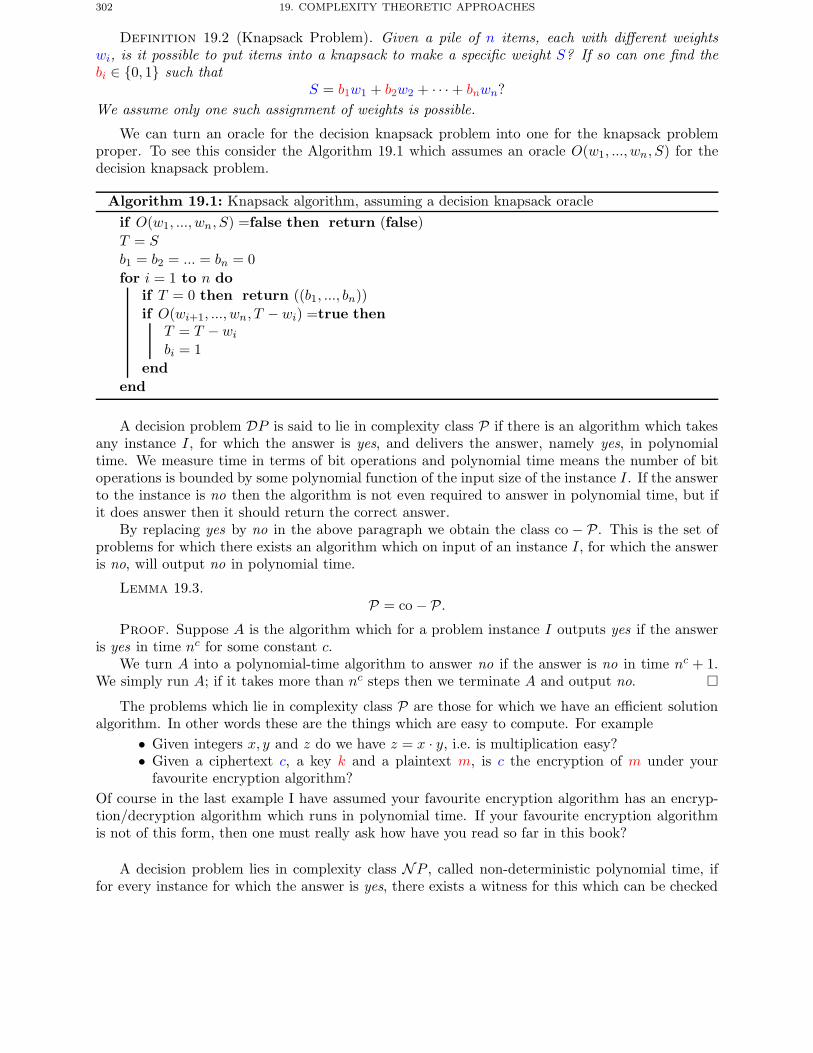
302 19. COMPLEXITY THEORETIC APPROACHES
Definition 19.2 (Knapsack Problem). Given a pile of n items, each with different weightswi, is it possible to put items into a knapsack to make a specific weight S? If so can one find thebi ∈ {0, 1} such that
S = b1w1 + b2w2 + · · · + bnwn?We assume only one such assignment of weights is possible.
We can turn an oracle for the decision knapsack problem into one for the knapsack problemproper. To see this consider the Algorithm 19.1 which assumes an oracle O(w1, ..., wn, S) for thedecision knapsack problem.
Algorithm 19.1: Knapsack algorithm, assuming a decision knapsack oracleif O(w1, ..., wn, S) =false then return (false)T = S
b1 = b2 = ... = bn = 0for i = 1 to n do
if T = 0 then return ((b1, ..., bn))if O(wi+1, ..., wn, T − wi) =true then
T = T − wibi = 1
endend
A decision problem DP is said to lie in complexity class P if there is an algorithm which takesany instance I, for which the answer is yes, and delivers the answer, namely yes, in polynomialtime. We measure time in terms of bit operations and polynomial time means the number of bitoperations is bounded by some polynomial function of the input size of the instance I. If the answerto the instance is no then the algorithm is not even required to answer in polynomial time, but ifit does answer then it should return the correct answer.
By replacing yes by no in the above paragraph we obtain the class co − P. This is the set ofproblems for which there exists an algorithm which on input of an instance I, for which the answeris no, will output no in polynomial time.
Lemma 19.3.P = co −P.
Proof. Suppose A is the algorithm which for a problem instance I outputs yes if the answeris yes in time nc for some constant c.
We turn A into a polynomial-time algorithm to answer no if the answer is no in time nc + 1.We simply run A; if it takes more than nc steps then we terminate A and output no. �
The problems which lie in complexity class P are those for which we have an efficient solutionalgorithm. In other words these are the things which are easy to compute. For example
• Given integers x, y and z do we have z = x · y, i.e. is multiplication easy?• Given a ciphertext c, a key k and a plaintext m, is c the encryption of m under your
favourite encryption algorithm?Of course in the last example I have assumed your favourite encryption algorithm has an encryp-tion/decryption algorithm which runs in polynomial time. If your favourite encryption algorithmis not of this form, then one must really ask how have you read so far in this book?
A decision problem lies in complexity class NP , called non-deterministic polynomial time, iffor every instance for which the answer is yes, there exists a witness for this which can be checked
1. POLYNOMIAL COMPLEXITY CLASSES 303
in polynomial time. If the answer is no we again do not assume the algorithm terminates, but if itdoes it must do so by answering no. One should think of the witness as a proof that the instanceI lies in the subset S.
Examples include• The problem ‘Is N composite?’ lies in NP as one can give a non-trivial prime factor as a
witness. This witness can be checked in polynomial time since division can be performedin polynomial time.
• The problem ‘Is G k-colourable?’ lies in NP since as a witness one can give the colouring.• The problem ‘Does this knapsack problem have a solution?’ lies in NP since as a witness
we can give the values bi.Note, in none of these examples have we assumed the witness itself can be computed in polynomialtime, only that the witness can be checked in polynomial time. Note that we trivially have
P ⊂ NP .
The main open problem in theoretical computer science is the question does P = NP? Most peoplebelieve in the conjecture
Conjecture 19.4.P �= NP .
The set co − NP is defined in the same way that the class co − P was derived from P. Theclass co−NP is the set of problems for which a witness exists for every instance with a no responsewhich can be checked in polynomial time. Unlike the case of co − P and P we have
If P �= NP then NP �= co −NP.
Hence, one should assume that NP �= co −NP.
One can consider trying to see how small a witness for being in class NP can be found. Forexample consider the problem COMPOSITES. Namely given N ∈ Z determine whetherN is composite.As we remarked earlier this clearly lies in class NP . But a number N can be proved composite inthe following ways:
• Giving a factor. In this case the size of the witness is
O(log n).
• Giving a Miller–Rabin witness a. Now, assuming the Generalized Riemann Hypothesis(GRH) the size of the witness is
O(log log n)
since we havea ≤ O((log n)2).
A decision problem DP is said to be NP -complete if every other problem in class NP can bereduced to this problem in polynomial time. In other words we have
DP ∈ P implies P = NP .
In some sense the NP -complete problems are the hardest problems for which it is feasible to askfor a solution. There are a huge number of NP -complete problems of which the two which willinterest us are
• the 3-colouring problem,• the knapsack problem.
304 19. COMPLEXITY THEORETIC APPROACHES
We know factoring (or COMPOSITES) lies in NP but it is unknown whether it is NP -complete.In fact it is a widely held view that all the hard problems on which cryptography is based, e.g.factoring, discrete logarithms etc., are not related to an NP -complete problem even though theylie in class NP .
From this we can conclude that factoring is not a very difficult problem at all, not at leastcompared with the knapsack problem or the 3-colouring problem. So why do we not use NP -complete problems on which to base our cryptographic schemes? These are after all a well-studiedset of problems for which we do not expect there ever to be an efficient solution.
However, this approach has had a bad track record, as we shall show later when we consider theknapsack based system of Merkle and Hellman. For now we simply mention that complexity theory,and so the theory of NP -completeness, is about worst case complexity. But for cryptography wewant a problem which, for suitably chosen parameters, is hard on average. It turns out that theknapsack problems that have in the past been proposed for use in cryptography are always ‘average’and efficient algorithms can always be found to solve them.
We end this section by illustrating this difference between hard and average problems usingthe k-colouring problem, when k = 3. Although determining whether a graph is 3-colourable is ingeneral (in the worst case) NP -complete, it is very easy on average. This is because the averagegraph, no matter how large it is, will not be 3-colourable. In fact, for almost all input graphs thefollowing algorithm will terminate saying that the graph is not 3-colourable in a constant numberof iterations.
• Take a graph G and order the vertices in any order v1, . . . , vt.• Call the colours {1, 2, 3}.• Now traverse the graph in the order of the vertices just decided.• On visiting a new vertex use the smallest possible colour (i.e. one from the set {1, 2, 3}
which does not appear as the colour of an adjacent vertex).• If you get stuck traverse back up the graph to the most recently coloured vertex and use
the next colour available, then continue again.• If at any point you run out of colours for the first vertex then terminate and say the graph
is not 3-colourable.• If you are able to colour the last vertex then terminate and output that the graph is
3-colourable.
The interesting thing about the above algorithm is that it can be shown that for a random graphof t vertices the average number of vertices travelled in the algorithm is less than 197 regardless ofthe number of vertices t in the graph.
2. Knapsack-Based Cryptosystems
One of the earliest public key cryptosystems was based on the knapsack, or subset sum, problemwhich was believed to be very hard in general to solve. In fact it is NP -complete, however it turnsout that this knapsack-based scheme, and almost all others, can be shown to be insecure.
The idea is to create two problem instances. A public one which is hard, which is believed tobe a general knapsack problem, and a private problem which is easy. In addition there should besome private trapdoor information which transforms the hard problem into the easy one.
This is rather like the use of the RSA assumption. It is hard to extract eth roots modulo acomposite number, but easy to extract eth roots modulo a prime number. Knowing the trapdoorinformation, namely the factorization of the RSA modulus, allows us to transform the hard probleminto the easy problem. However, the crucial difference is that whilst factoring (for suitably chosenmoduli) is hard on average, it is difficult to produce knapsack problems which are hard on average.
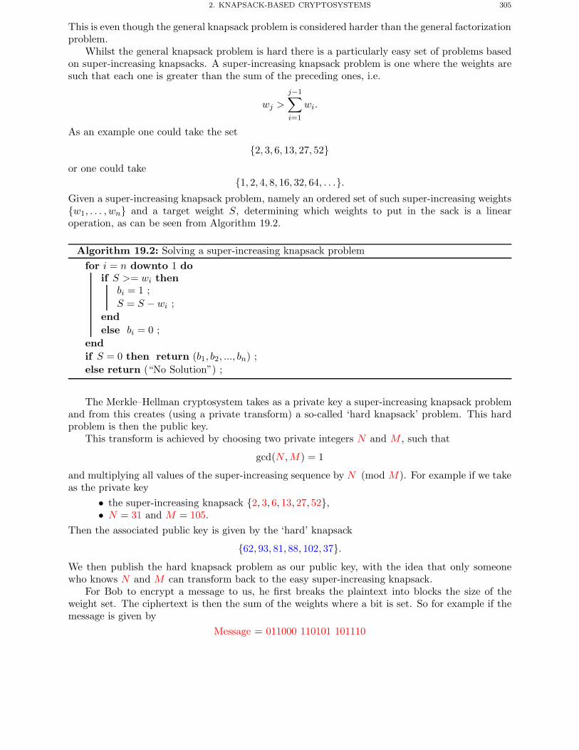
2. KNAPSACK-BASED CRYPTOSYSTEMS 305
This is even though the general knapsack problem is considered harder than the general factorizationproblem.
Whilst the general knapsack problem is hard there is a particularly easy set of problems basedon super-increasing knapsacks. A super-increasing knapsack problem is one where the weights aresuch that each one is greater than the sum of the preceding ones, i.e.
wj >
j−1∑i=1
wi.
As an example one could take the set
{2, 3, 6, 13, 27, 52}or one could take
{1, 2, 4, 8, 16, 32, 64, . . .}.Given a super-increasing knapsack problem, namely an ordered set of such super-increasing weights{w1, . . . , wn} and a target weight S, determining which weights to put in the sack is a linearoperation, as can be seen from Algorithm 19.2.
Algorithm 19.2: Solving a super-increasing knapsack problemfor i = n downto 1 do
if S >= wi thenbi = 1 ;S = S − wi ;
endelse bi = 0 ;
endif S = 0 then return (b1, b2, ..., bn) ;else return (“No Solution”) ;
The Merkle–Hellman cryptosystem takes as a private key a super-increasing knapsack problemand from this creates (using a private transform) a so-called ‘hard knapsack’ problem. This hardproblem is then the public key.
This transform is achieved by choosing two private integers N and M , such that
gcd(N,M ) = 1
and multiplying all values of the super-increasing sequence by N (mod M). For example if we takeas the private key
• the super-increasing knapsack {2, 3, 6, 13, 27, 52},• N = 31 and M = 105.
Then the associated public key is given by the ‘hard’ knapsack
{62, 93, 81, 88, 102, 37}.We then publish the hard knapsack problem as our public key, with the idea that only someonewho knows N and M can transform back to the easy super-increasing knapsack.
For Bob to encrypt a message to us, he first breaks the plaintext into blocks the size of theweight set. The ciphertext is then the sum of the weights where a bit is set. So for example if themessage is given by
Message = 011000 110101 101110
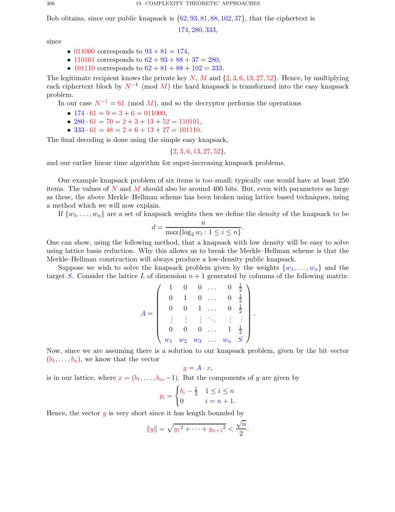
306 19. COMPLEXITY THEORETIC APPROACHES
Bob obtains, since our public knapsack is {62, 93, 81, 88, 102, 37}, that the ciphertext is
174, 280, 333,
since• 011000 corresponds to 93 + 81 = 174,• 110101 corresponds to 62 + 93 + 88 + 37 = 280,• 101110 corresponds to 62 + 81 + 88 + 102 = 333.
The legitimate recipient knows the private key N , M and {2, 3, 6, 13, 27, 52}. Hence, by multiplyingeach ciphertext block by N−1 (mod M) the hard knapsack is transformed into the easy knapsackproblem.
In our case N−1 = 61 (mod M), and so the decryptor performs the operations• 174 · 61 = 9 = 3 + 6 = 011000,• 280 · 61 = 70 = 2 + 3 + 13 + 52 = 110101,• 333 · 61 = 48 = 2 + 6 + 13 + 27 = 101110.
The final decoding is done using the simple easy knapsack,
{2, 3, 6, 13, 27, 52},and our earlier linear time algorithm for super-increasing knapsack problems.
Our example knapsack problem of six items is too small; typically one would have at least 250items. The values of N and M should also be around 400 bits. But, even with parameters as largeas these, the above Merkle–Hellman scheme has been broken using lattice based techniques, usinga method which we will now explain.
If {w1, . . . , wn} are a set of knapsack weights then we define the density of the knapsack to be
d =n
max{log2 wi : 1 ≤ i ≤ n} .One can show, using the following method, that a knapsack with low density will be easy to solveusing lattice basis reduction. Why this allows us to break the Merkle–Hellman scheme is that theMerkle–Hellman construction will always produce a low-density public knapsack.
Suppose we wish to solve the knapsack problem given by the weights {w1, . . . , wn} and thetarget S. Consider the lattice L of dimension n+ 1 generated by columns of the following matrix:
A =
⎛⎜⎜⎜⎜⎜⎜⎜⎜⎝
1 0 0 . . . 0 12
0 1 0 . . . 0 12
0 0 1 . . . 0 12
......
.... . .
......
0 0 0 . . . 1 12
w1 w2 w3 . . . wn S
⎞⎟⎟⎟⎟⎟⎟⎟⎟⎠.
Now, since we are assuming there is a solution to our knapsack problem, given by the bit vector(b1, . . . , bn), we know that the vector
y = A · x,is in our lattice, where x = (b1, . . . , bn,−1). But the components of y are given by
yi =
{bi − 1
2 1 ≤ i ≤ n
0 i = n+ 1.
Hence, the vector y is very short since it has length bounded by
‖y‖ =√y1
2 + · · · + yn+12 <
√n
2.
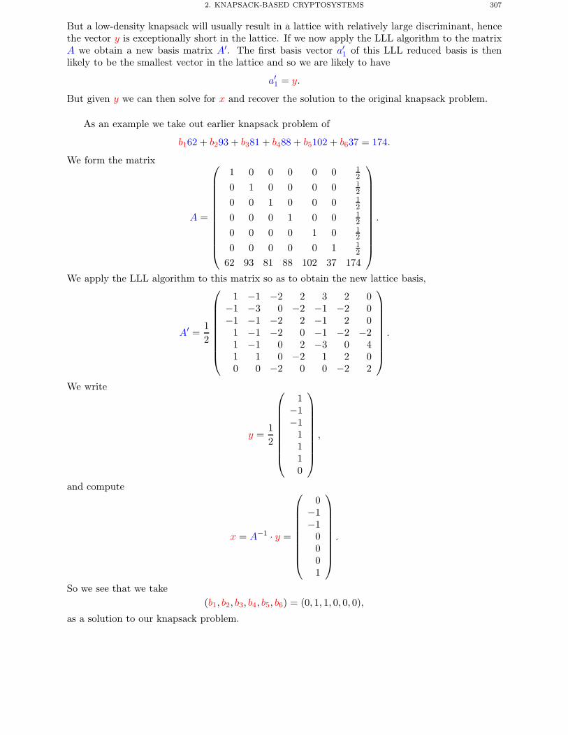
2. KNAPSACK-BASED CRYPTOSYSTEMS 307
But a low-density knapsack will usually result in a lattice with relatively large discriminant, hencethe vector y is exceptionally short in the lattice. If we now apply the LLL algorithm to the matrixA we obtain a new basis matrix A′. The first basis vector a′1 of this LLL reduced basis is thenlikely to be the smallest vector in the lattice and so we are likely to have
a′1 = y.
But given y we can then solve for x and recover the solution to the original knapsack problem.
As an example we take out earlier knapsack problem of
b162 + b293 + b381 + b488 + b5102 + b637 = 174.
We form the matrix
A =
⎛⎜⎜⎜⎜⎜⎜⎜⎜⎜⎜⎜⎝
1 0 0 0 0 0 12
0 1 0 0 0 0 12
0 0 1 0 0 0 12
0 0 0 1 0 0 12
0 0 0 0 1 0 12
0 0 0 0 0 1 12
62 93 81 88 102 37 174
⎞⎟⎟⎟⎟⎟⎟⎟⎟⎟⎟⎟⎠.
We apply the LLL algorithm to this matrix so as to obtain the new lattice basis,
A′ =12
⎛⎜⎜⎜⎜⎜⎜⎜⎜⎝
1 −1 −2 2 3 2 0−1 −3 0 −2 −1 −2 0−1 −1 −2 2 −1 2 0
1 −1 −2 0 −1 −2 −21 −1 0 2 −3 0 41 1 0 −2 1 2 00 0 −2 0 0 −2 2
⎞⎟⎟⎟⎟⎟⎟⎟⎟⎠.
We write
y =12
⎛⎜⎜⎜⎜⎜⎜⎜⎜⎝
1−1−1
1110
⎞⎟⎟⎟⎟⎟⎟⎟⎟⎠,
and compute
x = A−1 · y =
⎛⎜⎜⎜⎜⎜⎜⎜⎜⎝
0−1−1
0001
⎞⎟⎟⎟⎟⎟⎟⎟⎟⎠.
So we see that we take(b1, b2, b3, b4, b5, b6) = (0, 1, 1, 0, 0, 0),
as a solution to our knapsack problem.
308 19. COMPLEXITY THEORETIC APPROACHES
3. Bit Security
Earlier we looked at decision problems, i.e. those problems which output a single bit, andshowed that certain other non-decision problems, such as the knapsack problem, could be reducedto looking at decision problems only. A similar situation arises in cryptography where we wish toknow whether computing a single bit of information is as hard as computing all of the information.
For example suppose one is using the RSA function
x −→ y = xe (mod N).
It may be that in a certain system the attacker only cares about computing b = x (mod 2) andnot the whole of x. We would like it to be true that computing even this single bit of informationabout x is as hard as computing all of x. In other words we wish to study the so-called bit securityof the RSA function.
We can immediately see that bit security is related to semantic security. For example if anattacker could determine the parity of an underlying plaintext given only the ciphertext they couldeasily break the semantic security of the encryption algorithm.
First we define some notation:
Definition 19.5. Let f : S → T be a one-way function where S and T are finite sets and letB : S → {0, 1} denote a binary function (called a predicate). A hard predicate B(x) for f is onewhich is easy to compute given x ∈ S and for which it is hard to compute B(x) given only f(x).
The way one proves a predicate is a hard predicate, assuming f is a one-way function, is toassume we are given an oracle which computes B(x) given f(x), and then show that this oraclecan be used to easily invert f .
A k-bit predicate and hard k-bit predicate are defined in an analogous way but now assumingthe codomain of B is the set of bit strings of length k rather than just single bits. We would liketo show that various predicates, for given cryptographically useful functions f , are in fact hardpredicates.
3.1. Hard Predicates for Discrete Logarithms. Let G denote a finite abelian group ofprime order q and let g be a generator. Consider the predicate
B2 : x −→ x (mod 2)
we can show
Theorem 19.6. The predicate B2 is a hard predicate for the function
x −→ gx.
Proof. Let O(h, g) denote an oracle which returns the least significant bit of the discretelogarithm of h to the base g, i.e. it computes B2(x) for x = logg h. We need to show how to use Oto solve a discrete logarithm problem.
Suppose we are given h = gx, we perform the following steps. First we let t = 12 (mod q), then
we set y = 0, z = 1 and compute until h = 1 the following steps:• b = O(h, g).• If b = 1 then y = y + z and h = h/g.• Set h = ht and z = 2 · z.
We then output y as the discrete logarithm of h with respect to g. �
To see this work consider the field F607 and the element g = 64 of order q = 101. We wish tofind the discrete logarithm of h = 56 with respect to g. Using the algorithm in the above proof wecompute
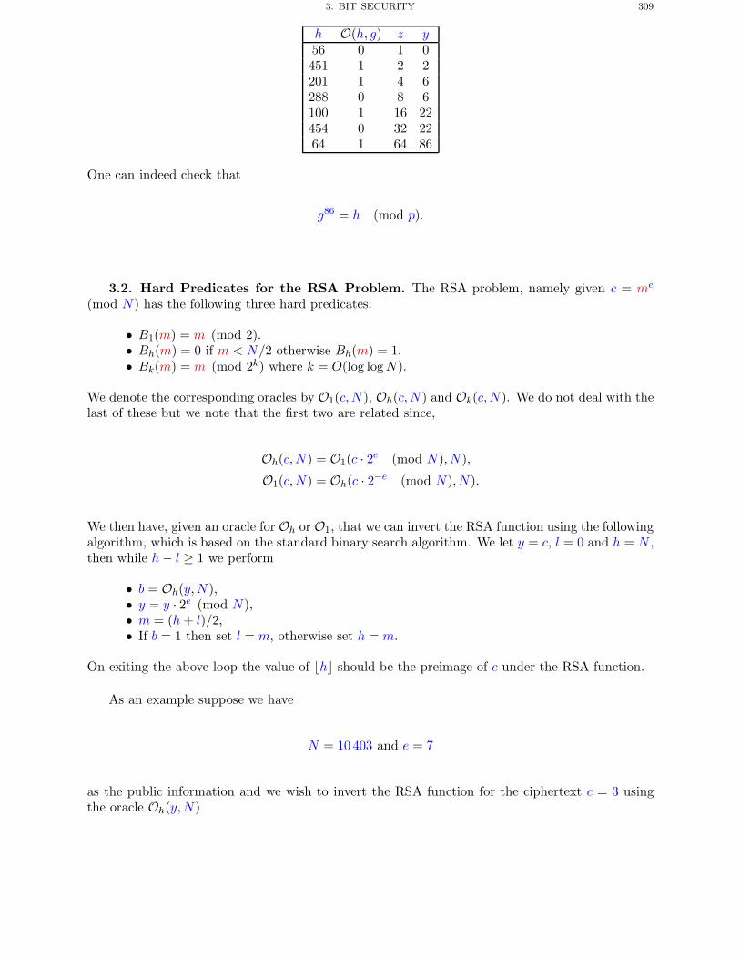
3. BIT SECURITY 309
h O(h, g) z y56 0 1 0451 1 2 2201 1 4 6288 0 8 6100 1 16 22454 0 32 2264 1 64 86
One can indeed check that
g86 = h (mod p).
3.2. Hard Predicates for the RSA Problem. The RSA problem, namely given c = me
(mod N) has the following three hard predicates:
• B1(m) = m (mod 2).• Bh(m) = 0 if m < N/2 otherwise Bh(m) = 1.• Bk(m) = m (mod 2k) where k = O(log logN).
We denote the corresponding oracles by O1(c,N ), Oh(c,N ) and Ok(c,N). We do not deal with thelast of these but we note that the first two are related since,
Oh(c,N) = O1(c · 2e (mod N),N ),
O1(c,N) = Oh(c · 2−e (mod N),N).
We then have, given an oracle for Oh or O1, that we can invert the RSA function using the followingalgorithm, which is based on the standard binary search algorithm. We let y = c, l = 0 and h = N ,then while h− l ≥ 1 we perform
• b = Oh(y,N ),• y = y · 2e (mod N),• m = (h+ l)/2,• If b = 1 then set l = m, otherwise set h = m.
On exiting the above loop the value of �h� should be the preimage of c under the RSA function.
As an example suppose we have
N = 10403 and e = 7
as the public information and we wish to invert the RSA function for the ciphertext c = 3 usingthe oracle Oh(y,N)
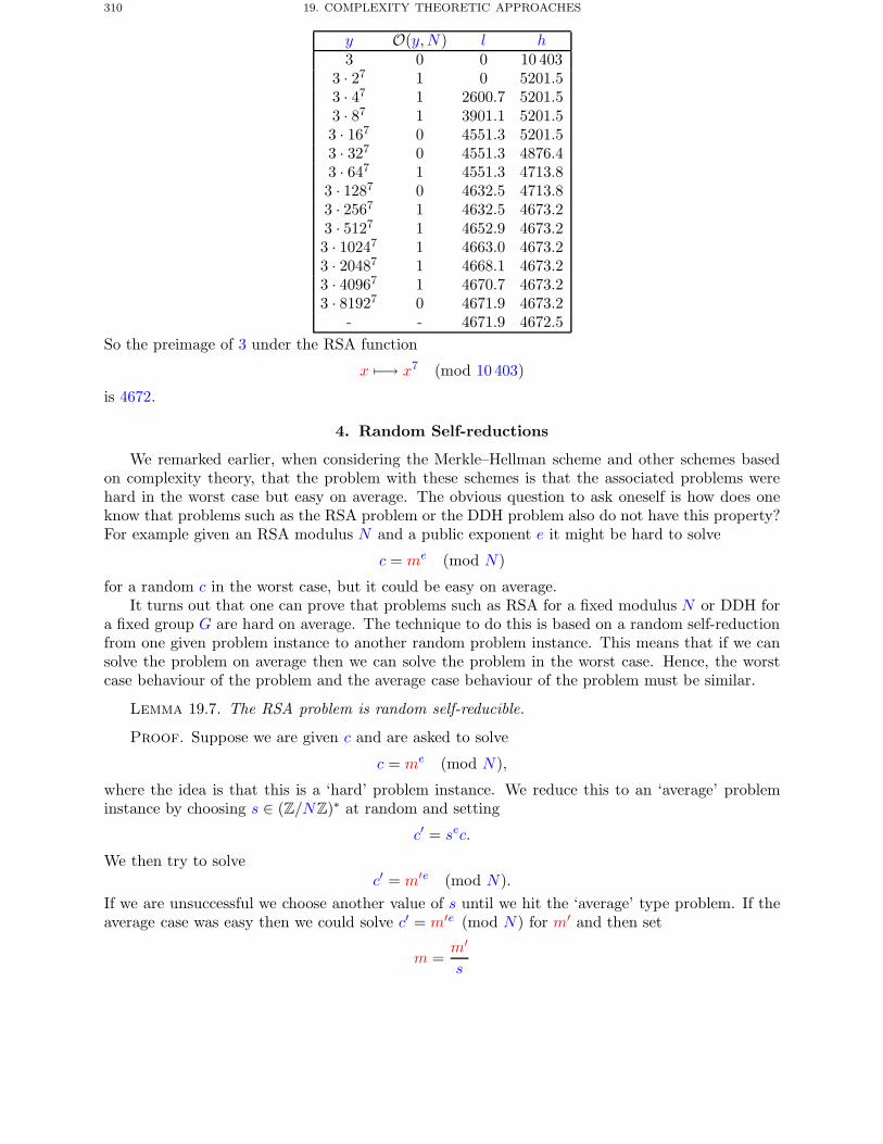
310 19. COMPLEXITY THEORETIC APPROACHES
y O(y,N) l h3 0 0 10 403
3 · 27 1 0 5201.53 · 47 1 2600.7 5201.53 · 87 1 3901.1 5201.53 · 167 0 4551.3 5201.53 · 327 0 4551.3 4876.43 · 647 1 4551.3 4713.83 · 1287 0 4632.5 4713.83 · 2567 1 4632.5 4673.23 · 5127 1 4652.9 4673.23 · 10247 1 4663.0 4673.23 · 20487 1 4668.1 4673.23 · 40967 1 4670.7 4673.23 · 81927 0 4671.9 4673.2
- - 4671.9 4672.5So the preimage of 3 under the RSA function
x −→ x7 (mod 10 403)
is 4672.
4. Random Self-reductions
We remarked earlier, when considering the Merkle–Hellman scheme and other schemes basedon complexity theory, that the problem with these schemes is that the associated problems werehard in the worst case but easy on average. The obvious question to ask oneself is how does oneknow that problems such as the RSA problem or the DDH problem also do not have this property?For example given an RSA modulus N and a public exponent e it might be hard to solve
c = me (mod N)
for a random c in the worst case, but it could be easy on average.It turns out that one can prove that problems such as RSA for a fixed modulus N or DDH for
a fixed group G are hard on average. The technique to do this is based on a random self-reductionfrom one given problem instance to another random problem instance. This means that if we cansolve the problem on average then we can solve the problem in the worst case. Hence, the worstcase behaviour of the problem and the average case behaviour of the problem must be similar.
Lemma 19.7. The RSA problem is random self-reducible.
Proof. Suppose we are given c and are asked to solve
c = me (mod N),
where the idea is that this is a ‘hard’ problem instance. We reduce this to an ‘average’ probleminstance by choosing s ∈ (Z/NZ)∗ at random and setting
c′ = sec.
We then try to solvec′ = m′e (mod N).
If we are unsuccessful we choose another value of s until we hit the ‘average’ type problem. If theaverage case was easy then we could solve c′ = m′e (mod N) for m′ and then set
m =m′
s
5. RANDOMIZED ALGORITHMS 311
and terminate. �
One can also show that the DDH problem is random self-reducible, in the sense that testingwhether
(x, y, z) = (ga, gb, gc)is a valid Diffie–Hellman triple, i.e. whether c = a · b, does not depend on the particular choices ofa, b and c. To see this consider the related triple
(x′, y′, z′) = (ga1 , gb1 , gc1) = (xvgu1 , ygu2 , zvyu1xvu2gu1u2)
for random u1, u2, v. Now if (x, y, z) is a valid Diffie–Hellman triplet then so is (x′, y′, z′), and viceversa.
One can show that the distribution of (x′, y′, z′) will be uniform over all valid Diffie–Hellmantriples if the original triple is a valid Diffie–Hellman triple, whilst the distribution will be uniformover all triples (and not just Diffie–Hellman ones) in the case where the original triple was not avalid Diffie–Hellman triple.
5. Randomized Algorithms
We end this chapter with a discussion of randomized algorithms; first we give some definitionsof algorithm types, then we relate these to complexity classes and finally we give some examples.
Recall that definitions are usually given for decision problems, so assume we have a propertywhich we wish to test to be true or false. There are the following definitions of algorithm types, alltaking their names from gambling cities.
• Monte-Carlo algorithm– Always outputs false if the answer is actually false– Answers true with probability ≥ 1/2.– Otherwise answers false, even though the actual answer is true.
• Atlantic City algorithm– Outputs true with probability ≥ 2/3 of being correct.– Outputs false with probability ≥ 2/3 of being correct.
• Las Vegas algorithm– Will terminate with the correct answer with probability ≥ 1/2.– Otherwise will not terminate.
In the above definitions we assume that the algorithm runs in polynomial time in terms of the sizeof the input data. We can clearly extend these definitions to non-decision problems quite easily.
We now turn our attention to the randomized complexity classes. We assume we have a probleminstance I and a possible witness w whose length is a polynomial function of the length of theinstance I. We wish to determine whether I ∈ S.
Definition 19.8. A problem DP is said to lie in class RP if there is an algorithm A, whichon input of a problem instance I and a witness w will perform as follows:
• If I ∈ S then for at least half of all possible witnesses w the algorithm A outputs thatI ∈ S.
• If I �∈ S then for all witnesses w the algorithm A outputs I �∈ S.
Note that we have, since we can replace ‘at least half’ with ‘at least one’, that
RP ⊂ NP.
We also clearly have P ⊂ RP .
312 19. COMPLEXITY THEORETIC APPROACHES
The class RP is important since it gives us a probabilistic algorithm to decide whether I ∈ Sfor any value of S. We generate k random witnesses wi and call A(I, wi) for i = 1, . . . , k. Then ifA(I, wi) returns I ∈ S for at least one value of wi then we return I ∈ S, otherwise we return I �∈ S.This latter statement will then be false around 1/2k of the time. Relating this to our definitionsbased on gambling cities we see that
If DP ∈ RP there exists a Monte-Carlo algorithm for DP .
We now define another class.
Definition 19.9. A problem DP is said to lie in class BPP if there is an algorithm A, whichon input of a problem instance I and a witness w will perform as follows:
• If I ∈ S then for at least 2/3 of all possible witnesses w the algorithm A outputs I ∈ S.• If I �∈ S then for at least 2/3 of all possible witnesses w the algorithm A outputs I �∈ S.
We see that
If DP ∈ BPP there exists an Atlantic City algorithm for DP .Finally we define the class ZPP as
ZPP = RP ∩ co −RP,
withIf DP ∈ ZPP there exists a Las Vegas algorithm for DP .
We have the inclusionsP ⊂ ZPP ⊂ RP ⊂ NP ∩ BPP.
The Fermat test and the Miller–Rabin test for primality are examples of Monte-Carlo algorithmsto test for compositeness. Recall these tests on input of a number N do one of two things:
• If N is prime will always output false (or probably prime).• If N is composite will output true with probability ≥ 1/2, otherwise will output false.
HenceCOMPOSITES ∈ RP .
By repeating the Monte-Carlo test we can amplify the probability of being correct to be arbitrarilyclose to one.
The Adleman–Huang algorithm for primality proving is an example of a Las Vegas algorithmto test for primality. The input to this problem is a number N . If the input is composite then thealgorithm may not terminate, but if it does terminate then it will tell us correctly whether N isprime or not. Hence
PRIMALITY ∈ ZPP .The historically earlier ECPP algorithm, on which the test of Adleman and Huang is based, is notguaranteed to terminate on input of a prime number, but in practice it always does.
Chapter Summary
• Complexity theory deals with the worst case behaviour of algorithms to solve a givendecision problem.
Further Reading 313
• Some problems are easy on average, but there exist certain instances which are very hardto solve. We do not wish to base our cryptographic systems on such problems.
• Cryptographic systems based on knapsack problems have been particularly notorious fromthis perspective, as one can often use lattice basis reduction to break them.
• Problems which we do base public key cryptography on, such as the RSA problem orthe discrete logarithm problem, have the property that even computing single bits of theanswer seems to be as hard as computing the whole answer.
• Problems such as RSA and the DDH problem are hard on average, since they possesrandom self-reductions from a given instance of the problem to a random instance of theproblem.
Further Reading
A nice introduction to complexity theory can be found in Chapter 2 of Bach and Shallit. Adiscussion of the relationships between theoretical complexity theory and cryptographic conceptssuch as zero-knowledge proofs can be found in the book by Goldreich. A discussion of knapsackbased systems and how to break them using lattices can be found in the survey article by Odlyzko.
E. Bach and S. Shallit. Algorithmic Number Theory, Volume 1: Efficient Algorithms. MIT Press,1996.
O. Goldreich. Modern Cryptography, Probabilistic Proofs and Pseudo-randomness. Springer-Verlag,1999.
A. Odlyzko. The Rise and Fall of Knapsack Cryptosystems. In Cryptology and ComputationalNumber Theory, Proc. Symposia in Applied Maths, Volume 42, 1990.

CHAPTER 20
Provable Security: With Random Oracles
Chapter Goals
• To describe the random oracle model.• To show how the random oracle model can be used to prove certain signature schemes are
secure.• To show why chosen ciphertext attacks require our public key encryption algorithms to
have redundancy in the ciphertext.• To explain RSA-OAEP and give a proof sketch.• To describe how to turn ElGamal encryption into a secure system.
1. Introduction
The modern approach to showing that certain protocols are secure is one based on provablesecurity. This name is in fact a misnomer since the techniques used do not actually prove security,in the sense of perfect security mentioned earlier. Instead, the proponents of provable security aimto prove that if an adversary is able to break a certain notion of the security of a system then onecould use the adversary to do something believed to be impossible.
For example one tries to prove that if one can break the semantic security of RSA in a chosenciphertext attack then one is also able to factor integers. Hence, such a proof is a relativized result,it is a proof of security relative to the hardness of factoring integers.
The major contribution of the area of provable security has really been in actually definingwhat is meant by a secure encryption or signature algorithm. Many of the concepts we havealready introduced such as existential forgery, semantic security, indistinguishability of encryptions,adaptive chosen ciphertext attacks have all arisen due to the study of provable security.
Let us explain the techniques of provable security by explaining what one means in a concreteexample. We suppose we are given an adversary which is a probabilistic algorithm which breakssome security property of RSA (for example semantic security of RSA) with a certain non-negligibleprobability. Already this leads us to some definitional work, what do we mean by non-negligibleprobability?
We hence need to define what we mean much better. We now assume that the scheme has asecurity parameter k, which measures how big the key size is. For example in RSA the securityparameter could be the number of bits in the modulus N . The adversary is said to be successfulwith non-negligible probability if it succeeds in its task with probability greater than
1/p(k),
where p is some polynomial in k.For the moment let us assume that our adversary A is a passive adversary, i.e. for RSA encryp-
tion it makes no decryption queries. We now wish to present a new algorithm BA which takes asinput an integer N and which calls the adversary a polynomial, in k, number of times. This new
315
316 20. PROVABLE SECURITY: WITH RANDOM ORACLES
algorithm’s aim could be to output the factors of N , with again a non-negligible probability. Thealgorithm BA would show that the existence of such an adversary A would imply a polynomial-timefactoring algorithm, which succeeded with a non-negligible probability. Since we do not believe apolynomial-time factoring algorithm is achievable with current knowledge we can conclude thatsuch an adversary is also unachievable with current knowledge.
You have already seen the above technique used when we showed that a successful passiveadversary against the ElGamal encryption scheme would imply an efficient algorithm to solve theDDH problem, or when we showed that a passive adversary against the Goldwasser–Micali schemewould imply an efficient algorithm to solve the QUADRES problem.
To recap, given an algorithm A we create a new algorithm BA which uses A as a subroutine.The input to BA is the hard mathematical problem we wish to solve, whilst the input to A is somecryptographic problem. The difficulty arises when A is an active adversary, in this case A is allowedto call a decryption or signature oracle for the input public keys. The algorithm BA, if it wants touse algorithm A as a subroutine, needs to supply the answers to A’s oracle queries. Algorithm BAnow has a number of problems:
• Its responses must appear valid, in that encryptions should decrypt and signatures shouldverify, otherwise algorithm A would notice its oracle was lying. Hence, algorithm BA couldno longer guarantee that algorithm A was successful with non-negligible probability.
• The responses of the oracle should be consistent with the probability distributions ofresponses that A expects if the oracles were true decryption/encryption oracles. Again,otherwise A would notice.
• The responses of the oracles should be consistent across all the calls made by the adversaryA.
• Algorithm BA needs to supply these answers without knowing the secret key. For examplein the case of RSA, if BA wants to find the factors of N , it can hardly use these factors torespond to algorithm A before it has found the factors.
This last point is the most crucial one. We are essentially asking BA to decrypt or sign a messagewithout knowing the private key, but this is meant to be impossible since our scheme is meant tobe secure.
To get around this problem it has become common practice to use something called the ‘randomoracle model’. A random oracle is an idealized hash function which on input of a new query willpick, uniformly at random, some response from its output domain, and which if asked the samequery twice will always return the same response.
In the random oracle model we assume our adversary A makes no use of the explicit hashfunction defined in the scheme under attack. In other words the adversary A runs, and is successful,even if we replace the real hash function by a random oracle. The algorithm BA responds to thedecryption oracle and/or signature queries of A by cheating and ‘cooking’ the responses of therandom oracle to suit his own needs. To see how this is done in practice look at the next sectionon proofs of security of signature algorithms.
A proof in the random oracle model is an even more relativized proof than that which weconsidered before. Such a proof says that assuming some problem is hard, say factoring, then anadversary cannot exist which makes no use of the underlying hash function. This does not implythat an adversary does not exist which uses the real specific hash function as a means of breakingthe cryptographic system.
In all our proofs and definitions we are very loose. We try to convey the flavour of the argumentsrather than the precise details. Those who want more precise definitions should look at the originalpapers. One should be warned however that in this field definitions can alter quite subtly from one
2. SECURITY OF SIGNATURE ALGORITHMS 317
paper to the next, this is because most of the real importance is in the definitions rather than theproofs themselves.
2. Security of Signature Algorithms
We first consider proofs of security of digital signature algorithms because they are conceptuallysomewhat simpler.
The first main technique we shall introduce is the forking lemma, due to Stern and Pointcheval.This applies to certain types of signature schemes which use a hash function as follows: To sign amessage
• the signer produces a, possibly empty, commitment σ1,• the signer computes h = H(σ1‖m),• the signer computes σ2 which is the ‘signature’ on σ1 and h.
We label the output of the signature schemes as (σ1,H(σ1‖m), σ2) so as to keep track of the exacthash query. For example we have
• DSA : σ1 = ∅, h = H(m),
σ2 = (r, (h+ xr)/k (mod q)) ,
where r =(gk (mod p)
)(mod q).
• EC-DSA : σ1 = ∅, h = H(m),
σ2 = (r, (h+ xr)/k (mod q)) ,
where r = x-coord([k]G).• Schnorr signatures: σ1 = gk, h = H(σ1‖m)
σ2 = xh+ k (mod q).
In all of these schemes the hash function is assumed to have codomain equal to Fq.
Recall in the random oracle model the hash function is allowed to be cooked up by the algorithmBA to do whatever it likes. Suppose an adversary A can produce an existential forgery on a messagem with non-negligible probability in the random oracle model. Hence, the output of the adversaryis
(m,σ1, h, σ2).We can assume that the adversary makes the critical hash query
h = H(σ1‖m),
since otherwise we can make the query for the adversary ourselves.Algorithm BA now runs the adversary A twice, with the same random tape and a slightly
different random oracle. The adversary A runs in polynomial time and so makes polynomiallymany hash queries. If all hash queries were answered the same as before then algorithm A wouldoutput exactly the same signature. However, algorithm BA answers these random oracle queriesjust as before, but chooses one hash query at random to answer differently. With non-negligibleprobability this will be the critical hash query and so (with non-negligible probability) the adversaryBA will obtain two signatures on the same message which have different hash query responses. Inother words we obtain
(m,σ1, h, σ2) and (m,σ1, h′, σ′2).
We then try to use these two outputs of algorithm A to solve the hard problem which is the goal ofalgorithm BA. The exact details and a thorough proof of this technique can be found in the paperby Stern and Pointcheval mentioned in the Further Reading section at the end of this chapter.
2.1. Passive Adversary Examples. We concern ourselves with some applications.
318 20. PROVABLE SECURITY: WITH RANDOM ORACLES
2.1.1. Schnorr Signatures: The technique of the forking lemma allows us to show
Theorem 20.1. In the random oracle model, assuming discrete logarithms are hard to computefor the group G, no passive adversary against Schnorr signatures can exist for the group G.
Proof. Let the input to algorithm BA be a discrete logarithm problem y = gx which we wishto solve. So let us assume we run our adversary A on input of the public key y and try to use theforking lemma argument. With non-negligible probability we obtain two signatures(
m,σ1 = gk, h, σ2 = xh+ k (mod q))
and (m,σ′1 = gk
′, h′, σ′2 = xh′ + k′ (mod q)
),
where h = H(σ1‖m) is the oracle query from the first run of A and h′ = H(σ′1‖m) is the oraclequery from the second run of A.
The algorithm BA’s goal is to recover x. It concludes that we must have k = k′ since we haveσ1 = σ′1. So it concludes that
Ax = B (mod q),where
A = h− h′ (mod q),
B = σ2 − σ′2 (mod q).
It will also know that A �= 0, since otherwise the two hash values would be equal. This then meansthat BA can solve the required discrete logarithm problem by computing
x = A−1B (mod q).
�
We shall later show that Schnorr signatures are also secure against active adversaries in therandom oracle model.
2.1.2. DSA Signatures: The above argument for Schnorr signatures does not apply to DSA aswe shall now show.
Let the input to algorithm BA be a discrete logarithm problem y = gx which we wish to solve.So let us assume we run our adversary A on input of the public key y and try to use the forkinglemma argument. With non-negligible probability we obtain two signatures
(m,σ1 = ∅, h, σ2 = (r, s)) and (m,σ′1 = ∅, h′, σ′2 = (r′, s′)),
where h = H(m) is the oracle query from the first run of A, h′ = H(m) is the oracle query fromthe second run of A and
r = gk (mod p) (mod q),
r′ = gk′
(mod p) (mod q),
s = (h+ xr)/k (mod q),
s′ = (h′ + xr′)/k′ (mod q).
The algorithm BA’s goal is to recover x. We can no longer conclude that k = k′, since we do noteven know that r = r′. Hence, the proof technique does not apply. In fact there is no known proofof security for DSA signatures.
We can try and repair this by using a modified form of DSA by applying the hash function tom and r instead of just m. In the context of the notation used in our description of the forkinglemma this would imply that σ1 = r, h = H(m‖r) and σ2 = (h+ xr)/k (mod q).
2. SECURITY OF SIGNATURE ALGORITHMS 319
Even with this modification, to make DSA more like Schnorr signatures, we cannot provesecurity. Our forking lemma argument would imply that we obtain two signatures with
r = gk (mod p) (mod q),
r′ = gk′
(mod p) (mod q),
s = (h+ xr)/k (mod q),
s′ = (h′ + xr′)/k′ (mod q),
and with r = r′. But we still could not imply that k = k′ since this does not follow from theequation
gk (mod p) (mod q) = gk′
(mod p) (mod q).It is the reduction modulo q which is getting in the way, if we removed this then our signaturescheme could be shown to be secure. But we would lose the property of small signature size whichDSA has.
2.1.3. EC-DSA Signatures: A similar problem arises with EC-DSA and the forking lemmaargument. But now a small modification allows us to give a proof of security for the modifiedscheme, in certain situations. We again assume that we apply the hash function to m and r insteadof just m. We then obtain by running our adversary twice and using the forking lemma
r = x-coord([k]P ) (mod q),
r′ = x-coord([k′]P ) (mod q),
s = (h+ xr)/k (mod q),
s′ = (h′ + xr′)/k′ (mod q),
where again we have r = r′ and h = H(m‖r) and h′ = H(m‖r′) are the two critical hash queries.If q is larger than the size of the finite field, from r = r′ we can now conclude that k = ±k′ and sowe deduce that
(s∓ s′)k = h− h′ (mod q).We therefore obtain two possibilities for k and we recover two possibilities for x. The actual answeris produced by checking which one of our two possibilities for x satisfies [x]P = Y . So we haveshown:
Theorem 20.2. In the random oracle model the above modified version of EC-DSA is secureagainst passive adversaries, assuming that the discrete logarithm problem in E(Fp) is hard and
q = #E(Fp) > p.
Notice how this result only applies to a certain subset of all elliptic curves.
2.2. Active Adversaries. To provide a proof for active adversaries we need to show howthe algorithm BA will answer the signature queries of the algorithm A. To do this we use therandom oracle model again, in that we use the ability of BA to choose the output of the hashfunction. Notice that this may mean that the input to the hash function must be unknown up untilthe message is signed. If the hash function is only applied to the message m and not some otherquantity (such as σ1 above) then algorithm A could have already queried the hash oracle for theinput m before the signature is created, and then algorithm BA would not be able to change theresponse from the previous one.
The process of BA signing signatures for A without A being able to tell and without BA havingthe private key is called a simulation of the signing queries. This simulation essentially means thatan active attack can be no more powerful than a passive attack, in the random oracle model, sinceany active attacker can be turned into a passive attacker by simply simulating the signing queries.
320 20. PROVABLE SECURITY: WITH RANDOM ORACLES
2.2.1. Schnorr Signatures: Providing a simulation of the signing queries for Schnorr signa-tures is particularly easy, and the simulator is closely related to our zero-knowledge protocols ofChapter 25. We assume that the simulator keeps a list L of all previous random oracle queries. Oninput of a message m the simulator does the following:
(1) Computes random values of s and h such that 1 ≤ s, h < q.(2) Sets r = gsy−h.(3) If (r‖m,h′) ∈ L for h′ �= h then the simulator returns to step 1.(4) Sets L = L∪ (r‖m,h), i.e. the hash oracle should now always return h on input of (r‖m).(5) Output the ‘signature’ (h, s).
You should check that the above does produce a valid signature, and that assuming h is a randomoracle the above simulation cannot be distinguished by algorithm A from a true signature algorithm.Hence we have:
Theorem 20.3. In the random oracle model, assuming discrete logarithms are hard to computefor the group G, no active adversary against Schnorr signatures can exist for the group G.
No similar security statement is known for DSA. A security proof is known for EC-DSA where,instead of modelling the hash function as a generic object and reducing the security to a discretelogarithm problem, one models the group operation as a generic object and reduces the security ofEC-DSA to the collision resistance of the actual hash function used.
2.3. RSA with Full Domain Hash. One should notice that in the previous discussion of theSchnorr, DSA and EC-DSA signature schemes we assumed that the hash function H is a functionwith codomain Fq. Such hash functions are hard to construct in practice, but the above argumentsassume this property.
A similar situation occurs with a variant of RSA signatures called RSA-FDH, or full domainhash. In this we assume a hash function
H : {0, 1}∗ −→ (Z/NZ)∗,
where N is the RSA modulus. Again such hash functions are hard to construct in practice, but ifwe assume they can exist and we model them by a random oracle then we can prove the followingRSA signature algorithm is secure.
Let N denote an RSA modulus with public exponent e and private exponent d. Let f denotethe function
f :{
(Z/NZ)∗ −→ (Z/NZ)∗
x −→ xe.
The RSA problem is given y = f(x) determine x. In the RSA-FDH signature algorithm on beinggiven a message m we produce the signature
s = H(m)d = f−1(H(m)).
One can then prove the following theorem.
Theorem 20.4. In the random oracle model if an active adversary A exists which produces anexistential forgery for RSA-FDH, which requires qH hash queries and qS signature queries, thenthere is an algorithm which given y can invert the RSA function on y with probability 1/qH .
Proof. We describe an algorithm BA which on input of y ∈ (Z/NZ)∗ outputs x = f−1(y).Algorithm BA first chooses a value of t ∈ [1, . . . , qH ] and throughout keeps a numbered record ofall the hash queries made. Algorithm BA runs algorithm A and responds to the hash queries forthe input mi as follows:
• If A makes a hash query, and this is the tth such query then BA replies with y and updatesthe internal hash list so that y = H(mt).
2. SECURITY OF SIGNATURE ALGORITHMS 321
• If A makes a hash query mi with i �= t, then BA computes a random si ∈ (Z/NZ)∗ andupdates the internal hash list so that H(mi) = sei (mod N) = hi, keeping a record of thevalue of si. Algorithm BA then responds with hi.
If A makes a signing query for a message mi before making a hash query on the message mi thenBA first makes the hash query for algorithm A. Then signing queries are responded to as:
• If message mi is equal to mt then algorithm BA stops and returns fail.• If mi �= mt then BA returns si as a response to the signature query.
Let A terminate with output (m, s) and without loss of generality we can assume that A made ahash oracle query for the message m. Now if m �= mt then BA terminates and admits failure. Butif m = mt then we have
f(s) = H(mt) = y.
Hence we have succeeded in inverting f .In analysing algorithm BA one notices that if A terminates successfully then (m, s) is an ex-
istential forgery and so m was not asked of the signing oracle. The value of t is independent ofthe view of A, so A cannot try and always ask for the signature of message mt in the algorithmrather than not ask for the signature. Hence, roughly speaking, the probability of success is around1/qH , i.e. the probability that the existential forgery was on the message mt and not on some otherone. �
2.4. RSA-PSS. Another way of securely using RSA as a signature algorithm is to use asystem called RSA-PSS, or probabilistic signature scheme. This scheme can also be proved securein the random oracle model under the RSA assumption. We do not give the details of the proofhere but simply explain the scheme, since it is becoming increasingly important due to its adoptionby standards bodies. The advantage of RSA-PSS over RSA-FDH is that one only requires a hashfunction with a traditional codomain, e.g. bit strings of length t, rather than a set of integersmodulo another number.
As usual one takes an RSA modulus N , a public exponent e and a private exponent d. Supposethe security parameter is k, i.e. N is a k bit number. We define two integers k0 and k1 so that
k0 + k1 ≤ k − 1.
For example one could take ki = 128 or 160.We then define two hash functions, one which expands data and one which compresses data:
G : {0, 1}k1 −→ {0, 1}k−k1−1
H : {0, 1}∗ −→ {0, 1}k1 .We let
G1 : {0, 1}k1 −→ {0, 1}k0denote the function which returns the first k0 bits of G(w) for w ∈ {0, 1}k1 and we let
G2 : {0, 1}k1 −→ {0, 1}k−k0−k1−1
denote the function which returns the last k − k0 − k1 − 1 bits of G(w) for w ∈ {0, 1}k1 . To sign amessage m:
• Generate a random value r ∈ {0, 1}k0 .• Put w = H(m‖r).• Set y = 0‖w‖(G1(w) ⊕ r)‖G2(w).• Output s = yd (mod N).
To verify a signature (s,m):• Compute y = se (mod N).
322 20. PROVABLE SECURITY: WITH RANDOM ORACLES
• Split y into the componentsb‖w‖α‖γ
where b is one bit long, w is k1 bits long, α is k0 bits long and γ is k − k0 − k1 − 1 bitslong.
• Compute r = α⊕G1(w).• The signature verifies if
b = 0 and G2(w) = γ and H(m‖r) = w.
If we allow the modelling of the hash functions G and H by random oracles then one can show thatthe above signature algorithm is secure, in the sense that the existence of a successful algorithm tofind existential forgeries could be used to produce an algorithm to invert the RSA function. Forthe proof of this one should consult the EuroCrypt ’96 paper of Bellare and Rogaway mentionedin the Further Reading section at the end of this chapter.
3. Security of Encryption Algorithms
We have seen that it is easy, under the DDH assumption, to produce semantically secure publickey encryption schemes assuming only passive adversaries. For example the ElGamal encryptionscheme satisfies these properties. We have also seen that a semantically secure system based onthe QUADRES problem is easy to produce, assuming only passive adversaries, but this system ofGoldwasser and Micali has terrible message expansion properties. It is much harder to produce dis-crete logarithm based systems which are secure against active adversaries or which are semanticallysecure under the RSA assumption.
In this section we first present some historical attempts at producing ElGamal based encryptionalgorithms which aimed to be secure against active adversaries. These are important as they showa basic design criteria. We then go on to describe the main RSA based system which is secureagainst active adversaries in the random oracle model, namely RSA-OAEP.
3.1. Immunization of ElGamal Based Encryption. Recall that ElGamal encryption isgiven by
(gk,m · yk)where y = gx is the public key. Such a system can be proved to have semantic security under theDDH assumption using quite elementary techniques, as we showed in Chapter 18. However, wealso showed that such a system is not secure against active adversaries since the ciphertext wastrivially malleable.
It was soon realized that the problem with active attacks was that it was too easy for theadversary to write down a valid ciphertext, and not just a related one. The reasoning went that ifit was hard for the adversary to write down a valid ciphertext without having first encrypted theplaintext to produce the ciphertext, then the adversary would have no advantage in mounting achosen ciphertext attack. After all, why would an adversary want to decrypt a ciphertext if theonly way he could produce a ciphertext was to encrypt some plaintext?
This meant one needed a decryption function which on input of a ciphertext would eitheroutput the corresponding plaintext or would output the ⊥ symbol, to signal an Invalid Ciphertext.For this to happen some redundancy needs to be added to the ciphertext which could be checkedby the decryptor, to check whether the ciphertext was valid. Compare this with our discussion onencryption functions in Chapter 5, where we argued that a ciphertext should contain no redundancy.But there we were only interested in passive attacks, here we are trying to defend against muchmore powerful adversaries.
Zheng and Seberry were the first to explore this philosophy for practical cryptosystems, whichpervades the modern approach to public key encryption function design. Their overall approach is
3. SECURITY OF ENCRYPTION ALGORITHMS 323
important, so we present these early attempts at producing secure public key encryption schemesas illustrative of the approach.
The first thing to notice is that public key encryption is usually used to convey a key to encrypta large message, hence it is not necessary to encrypt a message which lies in the group G (as inElGamal encryption). We can still use the ElGamal idea to transport a key, which we can then useto produce a session key to encrypt the actual message.
We first describe some notation:• G is a public group of prime order q generated by g.• V (h) takes a group element h and generates a random bit string from h. The function V
is often called a key derivation function.• H is a hash function producing an l-bit output.• y = gx will be the public key corresponding to the private key x.
3.1.1. Zheng–Seberry Scheme 1: To encrypt a message m one computes(1) k ∈R {1, . . . , q − 1}.(2) z = V (yk).(3) t = H(m).(4) c1 = gk.(5) c2 = z ⊕ (m‖t).(6) Output (c1, c2).
When we decrypt a ciphertext we perform the following steps(1) z′ = V (c1x).(2) w = z′ ⊕ c2.(3) t′ is the last l bits of w.(4) m′ is the first #w − l bits of w.(5) If H(m′) = t′ then output m′.(6) Output ⊥.
The idea here is that we have added an extra piece of information to the ElGamal ciphertext,namely the encryption of the hash of the plaintext. Since it is meant to be hard to invert the hashfunction it should be hard to write down a valid ciphertext without knowing the correspondingplaintext. The addition of the hash adds the required redundancy which is then tested by thedecryption function.
3.1.2. Zheng–Seberry Scheme 2: The second system uses a universal one-way hash function,which is essentially a parametrized set of hash functions Hi, where i ≤ �. One can think of this insome ways as a keyed hash function or as a MAC.
More formally a universal one-way hash function is a keyed hash function Hk such that if theadversary is given x and then a hidden key k is chosen at random it should be hard for the adversaryto be able to compute a y such that
Hk(y) = Hk(x).To encrypt a message m in the second of Zheng and Seberry’s schemes we compute
(1) k ∈R {1, . . . , q − 1}.(2) Let z denote the #m leftmost bits of V (yk).(3) Let s denote the � rightmost bits of V (yk).(4) c1 = gk.(5) c2 = Hs(m).(6) c3 = z ⊕m.(7) Output (c1, c2, c3).
We leave it to the reader to write down the associated decryption function. The above system issimilar to the first but the hash of the message is no longer encrypted, it is now sent in the clear.
324 20. PROVABLE SECURITY: WITH RANDOM ORACLES
But now one has an added difficultly since we do not know which hash function, or key, has beenused to generate the hash value. The above system is very close to the system called DHIES whichis currently considered the best practical algorithm based on ElGamal encryption.
3.1.3. Zheng–Seberry Scheme 3: In the third and final scheme produced by Zheng and Seberryone uses a DSA-like signature to ‘sign’ the message which is encrypted. The scheme works like acombination of an ElGamal-like encryption followed by a DSA signature, however the public keyfor the DSA signature is ephemeral and becomes part of the ciphertext. Again we leave it for thereader to write down the decryption algorithm.
(1) k, t ∈R {1, . . . , q − 1}.(2) r = yk+t.(3) z = V (r).(4) c1 = gk.(5) c2 = gt.(6) c3 = (H(m) + xr)/k (mod q).(7) c4 = z ⊕m.(8) Output (c1, c2, c3, c4).
Zheng and Seberry proved their schemes secure under a very strong conjectural assumption,namely that the space of ciphertexts was ‘sole samplable’. This is an assumption akin to assumingthat the encryption algorithm is plaintext aware. However, the first of the above schemes can beshown to be trivially insecure as follows. Suppose in the find stage our adversary outputs twomessages m1 and m2. Then a hidden bit b is chosen and the adversary is given the encryption ofmb. This is equal to
c = (c1, c2) =(gk, z ⊕ (mb‖H(mb))
).
The adversary in its guess stage can now perform the following operations. First it generates anew message m3, different from m1 and m2, but of the same length. Then the adversary asks thedecryption oracle to decrypt the ciphertext
(c1, c2 ⊕ (m1‖H(m1)) ⊕ (m3‖H(m3))) .
When b = 1 the above ciphertext will be a valid encryption of m3 and so the decryption oracle willreturn m3. However, when b = 0 the above ciphertext is highly unlikely to be a valid encryption ofanything, let alone m3. This gives us a polynomial-time test, for an adaptive adversary, to detectthe value of the hidden bit b.
3.2. RSA-OAEP. Recall that the raw RSA function does not provide a semantically secureencryption scheme, even against passive adversaries. To make a system which is secure we needeither to add redundancy to the plaintext before encryption or to add some other form of re-dundancy to the ciphertext. In addition the padding used needs to be random so as to make anon-deterministic encryption algorithm. This is done in RSA by using a padding scheme, and overthe years a number of padding systems have been proposed. However, some of the older ones arenow considered weak.
By far the most successful padding scheme in use today was invented by Bellare and Rogawayand is called OAEP or Optimized Asymmetric Encryption Padding. OAEP is a padding schemewhich can be used with any function which is a one-way trapdoor permutation, in particular theRSA function. When used with RSA it is often denoted RSA-OAEP.
Originally it was thought the RSA-OAEP was a plaintext-aware encryption algorithm, but thisclaim has since been shown to be wrong. However, one can show in the random oracle model thatRSA-OAEP is semantically secure against adaptive chosen ciphertext attacks.
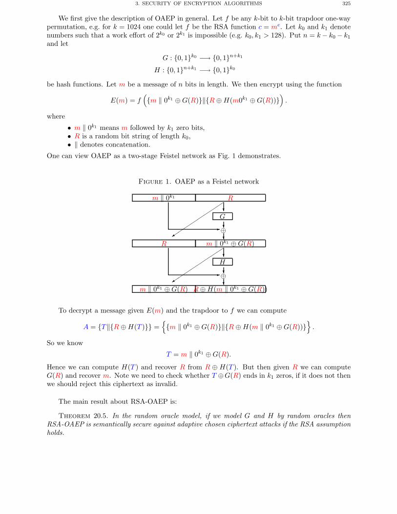
3. SECURITY OF ENCRYPTION ALGORITHMS 325
We first give the description of OAEP in general. Let f be any k-bit to k-bit trapdoor one-waypermutation, e.g. for k = 1024 one could let f be the RSA function c = me. Let k0 and k1 denotenumbers such that a work effort of 2k0 or 2k1 is impossible (e.g. k0, k1 > 128). Put n = k− k0 − k1
and let
G : {0, 1}k0 −→ {0, 1}n+k1
H : {0, 1}n+k1 −→ {0, 1}k0
be hash functions. Let m be a message of n bits in length. We then encrypt using the function
E(m) = f({m ‖ 0k1 ⊕G(R)}‖{R ⊕H(m0k1 ⊕G(R))}
).
where
• m ‖ 0k1 means m followed by k1 zero bits,• R is a random bit string of length k0,• ‖ denotes concatenation.
One can view OAEP as a two-stage Feistel network as Fig. 1 demonstrates.
Figure 1. OAEP as a Feistel network
m ‖ 0k1 R�
��
��
��
��
G
⊕
R m ‖ 0k1 ⊕G(R)�
��
��
��
��
H
⊕
m ‖ 0k1 ⊕G(R) R⊕H(m ‖ 0k1 ⊕G(R))
To decrypt a message given E(m) and the trapdoor to f we can compute
A = {T‖{R ⊕H(T )}} ={{m ‖ 0k1 ⊕G(R)}‖{R ⊕H(m ‖ 0k1 ⊕G(R))}
}.
So we know
T = m ‖ 0k1 ⊕G(R).
Hence we can compute H(T ) and recover R from R ⊕ H(T ). But then given R we can computeG(R) and recover m. Note we need to check whether T ⊕G(R) ends in k1 zeros, if it does not thenwe should reject this ciphertext as invalid.
The main result about RSA-OAEP is:
Theorem 20.5. In the random oracle model, if we model G and H by random oracles thenRSA-OAEP is semantically secure against adaptive chosen ciphertext attacks if the RSA assumptionholds.
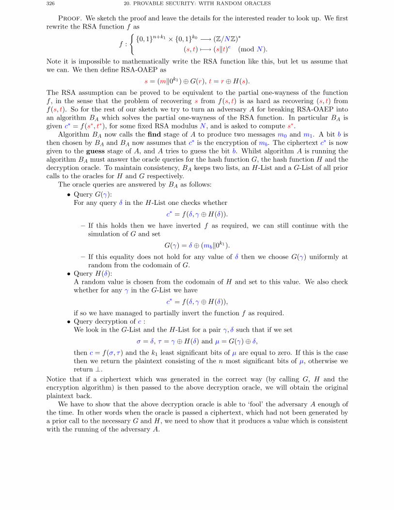
326 20. PROVABLE SECURITY: WITH RANDOM ORACLES
Proof. We sketch the proof and leave the details for the interested reader to look up. We firstrewrite the RSA function f as
f :
{{0, 1}n+k1 × {0, 1}k0 −→ (Z/NZ)∗
(s, t) −→ (s‖t)e (mod N).
Note it is impossible to mathematically write the RSA function like this, but let us assume thatwe can. We then define RSA-OAEP as
s = (m‖0k1) ⊕G(r), t = r ⊕H(s).
The RSA assumption can be proved to be equivalent to the partial one-wayness of the functionf , in the sense that the problem of recovering s from f(s, t) is as hard as recovering (s, t) fromf(s, t). So for the rest of our sketch we try to turn an adversary A for breaking RSA-OAEP intoan algorithm BA which solves the partial one-wayness of the RSA function. In particular BA isgiven c∗ = f(s∗, t∗), for some fixed RSA modulus N , and is asked to compute s∗.
Algorithm BA now calls the find stage of A to produce two messages m0 and m1. A bit b isthen chosen by BA and BA now assumes that c∗ is the encryption of mb. The ciphertext c∗ is nowgiven to the guess stage of A, and A tries to guess the bit b. Whilst algorithm A is running thealgorithm BA must answer the oracle queries for the hash function G, the hash function H and thedecryption oracle. To maintain consistency, BA keeps two lists, an H-List and a G-List of all priorcalls to the oracles for H and G respectively.
The oracle queries are answered by BA as follows:• Query G(γ):
For any query δ in the H-List one checks whether
c∗ = f(δ, γ ⊕H(δ)).
– If this holds then we have inverted f as required, we can still continue with thesimulation of G and set
G(γ) = δ ⊕ (mb‖0k1).– If this equality does not hold for any value of δ then we choose G(γ) uniformly at
random from the codomain of G.• Query H(δ):
A random value is chosen from the codomain of H and set to this value. We also checkwhether for any γ in the G-List we have
c∗ = f(δ, γ ⊕H(δ)),
if so we have managed to partially invert the function f as required.• Query decryption of c :
We look in the G-List and the H-List for a pair γ, δ such that if we set
σ = δ, τ = γ ⊕H(δ) and μ = G(γ) ⊕ δ,
then c = f(σ, τ) and the k1 least significant bits of μ are equal to zero. If this is the casethen we return the plaintext consisting of the n most significant bits of μ, otherwise wereturn ⊥.
Notice that if a ciphertext which was generated in the correct way (by calling G, H and theencryption algorithm) is then passed to the above decryption oracle, we will obtain the originalplaintext back.
We have to show that the above decryption oracle is able to ‘fool’ the adversary A enough ofthe time. In other words when the oracle is passed a ciphertext, which had not been generated bya prior call to the necessary G and H, we need to show that it produces a value which is consistentwith the running of the adversary A.
Chapter Summary 327
Finally we need to show that if the adversary A has a non-negligible chance of breaking thesemantic security of RSA-OAEP then one has a non-negligible probability that BA can partiallyinvert f .
These last two facts are proved by careful analysis of the probabilities associated with a numberof events. Recall that BA assumes that c∗ = f(s∗, t∗) is an encryption of mb. Hence, there shouldexist an r∗ which satisfies
r∗ = H(s∗) ⊕ t∗,
G(r∗) = s∗ ⊕ (mb‖0k1).One first shows that the probability of the decryption simulator failing is negligible. Then oneshows that the probability that s∗ is actually asked of the H oracle is non-negligible, as long as theadversary A has a non-negligible probability of finding the bit b. But as soon as s∗ is asked of Hthen we spot this and can therefore break the partial one-wayness of f .
The actual technical probability arguments are rather involved and we refer the reader to thepaper of Fujisaki, Okamoto, Pointcheval and Stern where the full proof is given. �
3.3. Turning CPA Schemes into CCA2 Schemes. Suppose we have a public key en-cryption scheme which is semantically secure against chosen plaintext attacks, such as ElGamalencryption. Such a scheme by definition needs to be non-deterministic hence we write the encryp-tion function as
E(m, r),
where m is the message to be encrypted and r is the random input and we denote the decryptionfunction by D(c). Hence, for ElGamal encryption we have
E(m, r) = (gr,m · hr).Fujisaki and Okamoto showed how to turn such a scheme into an encryption scheme which is
semantically secure against adaptive adversaries. Their result only applies in the random oraclemodel and works by showing that the resulting scheme is plaintext aware. We do not go into thedetails of the proof at all, but simply give the transformation which is both simple and elegant.
We take the encryption function above and alter it by setting
E′(m, r) = E(m‖r,H(m‖r))where H is a hash function. The decryption algorithm is also altered in that we first compute
m′ = D(c)
and then we check thatc = E(m′,H(m′)).
If this last equation holds we recover m from m′ = m‖r, if the equation does not hold then wereturn ⊥.
For ElGamal encryption we therefore obtain the encryption algorithm
(gH(m‖r), (m‖r) · hH(m‖r)),
which is only marginally less efficient than raw ElGamal encryption.
Chapter Summary
328 20. PROVABLE SECURITY: WITH RANDOM ORACLES
• The main technique in provable security is to show how the existence of an adversaryagainst the cryptographic scheme under consideration can be used to solve some suppos-edly hard problem. Since one believes the problem to be hard, one then concludes thatsuch an adversary cannot exist.
• The random oracle model is a computational model used as a proof technique in provablesecurity. A proof in the random oracle model does not mean the system is secure in thereal world, it only provides evidence that it may be secure.
• In the random oracle model one can use the forking lemma to show that certain discretelogarithm signature schemes are secure. To obtain proofs in the case of active adversariesone uses the random oracle to simulate the signing queries of the adversary.
• One can also show in the random oracle model that the two main RSA based signatureschemes used in ‘real life’ are also secure, namely RSA-FDH and RSA-PSS.
• Proving encryption algorithms to be secure is slightly more tricky, early attempts of Zhengand Seberry made use of non-standard assumptions.
• In the random oracle model one can prove that the standard RSA encryption method,namely RSA-OAEP, is secure.
Further Reading
Provable security is a rapidly expanding field, and the number of papers grows with eachpassing year. A good description of the forking lemma and its applications is given in the articleof Pointcheval and Stern. The random oracle model and a number of applications including RSA-FDH and RSA-PSS are given in the papers of Bellare and Rogaway. The full proof of the securityof RSA-OAEP is given in the paper of Fujisaki and others.
M. Bellare and P. Rogaway. Random oracles are practical: a paradigm for designing efficientprotocols. In Proc. 1st Annual Conf. on Comp. and Comms. Security, ACM, 62–73, 1993.
M. Bellare and P. Rogaway. The exact security of digital signatures – How to sign with RSA andRabin. In Advances in Cryptology – EuroCrypt ’96. Springer-Verlag LNCS 1070, 399–416, 1996.
E. Fujisaki, T. Okamoto, D. Pointcheval and J. Stern. RSA-OAEP is secure under the RSAassumption. In Advances in Cryptology – CRYPTO 2001, Springer-Verlag LNCS 2139, 260–274,2001.
D. Pointcheval and J. Stern. Security arguments for digital signatures and blind signatures. J. Cryp-tology, 13, 361–396, 2000.

CHAPTER 21
Hybrid Encryption
Chapter Goals
• To introduce the security notions for symmetric encryption schemes.• To introduce and formalise the notion of hybrid encryption, via KEMs and DEMs.• To present an efficient DEM, built out of a block cipher and a MAC.• To present two efficient KEMs, namely RSA-KEM and DHIES.
1. Introduction
Almost always public key schemes are used to only transmit a short per message secret, such asa session key. This is because public key schemes are too inefficient to use to encrypt vast amountsof data. The actual data is then encrypted using a symmetric cipher. Such an approach is calleda hybrid encryption scheme.
In this chapter we first define the security notions for symmetric ciphers which are analogousto those presented in Chapter 18. This allows us to then go on and formalise a way of designinga hybrid cipher, using the KEM/DEM approach. A KEM is a Key Encapsulation Mechansism,which is the public key component of a hybrid cipher, whilst a DEM is the Data EncapsulationMechansism, which is the symmetric component. We show how a secure DEM can be formed froma weakly secure symmetric cipher and a MAC.
We then argue, without using random oracles, that a suitably secure DEM and a suitably secureKEM can be combined to produce a secure hybrid cipher. This means we only need to considerthe symmetric and public key parts seperately, thus simplifying our design considerably.
Finally, we show how a KEM can be constructed in the random oracle model using either theRSA or the DLP primitive. The resulting KEMs are very simple to construct and very natural,and thus we see the simplification we obtain by considering hybrid encryption.
2. Security of Symmetric Ciphers
In this section we extend the security model of semantic security under adaptive chosen cipher-text attack for public key schemes to the symmetric setting, we then look at what the securitydefinition should be for message authentication codes.
2.1. Security Models for Symmetric Ciphers. Semantic/polynomial security of symmet-ric ciphers is defined similarly to that of public key schemes. Let Ek(m) denote the encryptionalgorithm and Dk(c) denote the decryption algorithm.
The adversary runs in two stages:• Find: In the find stage the adversary produces two plaintext messages m0 and m1, of
equal length.• Guess: The adversary is now given the encryption cb = Ek(mb) of one of the plaintextsmb for some secret hidden bit b under some randomly chosen, and secret, symmetric key
329
330 21. HYBRID ENCRYPTION
k. The goal of the adversary is to guess the value of the bit b with probability greaterthan one half.
Note, that this does not mean, as it does in the public key setting, that the encryption schememust be probabilistic since the adversary is unable to evaluate the encryption algorithm withoutknowing the secret key k. Also, note that the key, under which the challeneg message is encrypted,is chosen after the adversary has chosen his two messages.
This type of security is often called one-time security, since the adversary only sees one validciphertext encrypted under the target key. This needs to be compared to the public key settingwhereby an adversary can generate as many valid ciphertexts of its choosing by simply encryptinga message using the public key.
The advantage of an adversary A in the above game is defined to be
AdvA =∣∣∣∣Pr(A(guess, cb,m0,m1) = b) − 1
2
∣∣∣∣ .A scheme is said to be secure if for all adversaries, all polynomials p and sufficiently large t we have
AdvA ≤ 1p(t)
,
where t is the key size of the symmetric cipher. We say that AdvA grows as a negligible functionof t.
Notice, that in the above game that the adversary only sees one encryption of a message underthe secret key k. Schemes which are secure in this sense are often called one-time encryptionschemes. Recall that in Chapter 8 we commented that sometimes one used CBC mode with a fixedIV , this is precisely the situation we have here. Hence, for one-time encryption schemes one canuse deterministic encryption.
To see a distinct difference between the public key and the private key setting, notice that in thepublic key setting the adversary could obtain encryptions of messages of her choice. This resultedin public key schemes needing to be probabilistic in nature. In the symmetric setting the adversaryis not able to obtain encryptions of messages of her choice, bar the encryption of mb. Thus we canuse deterministic symmetric encryption in this setting.
The above definition defines the notion of semantic security (or indistinguishability of encryp-tions) against passive attacks. It is clear that the one-time pad will meet the above securitydefinition. To define the notion for adaptive adversaries, i.e. CCA attacks, we give the adversarya decryption box in the second phase of the game which will decrypt, under the key k, arbitraryciphertexts c of her choosing. Except the adversary is not allowed to query the decryption boxwith the target ciphertext cb.
There are situations where one used a symmetric cipher in places where an adversary is ableto obtain encryptions of messages of their choice. Such a situation is said to be a chosen plaintexattack, i.e. CPA attack. Note, that in the symmetric setting a CPA attack is an active attackwhilst in the public key setting a CPA attack is a passive attack. In such situations the symmetriccipher needs to be probabilistic in nature. It is in these situations where one could use CBC Modewith a randomized IV .
It is assumed that a good block cipher used in CBC Mode produces a symmetric cipher which issemantically secure under passive attacks (fixed or random IV ) or chosen plaintext attacks (randomIV ). However, they do not produce ciphers which are secure under chosen ciphertext attacks asthe following example illustrates. Suppose the adversary selects two messages m1 and m2 of lengthtwice the block length of the underlying cipher, i.e. we write
m1 = m1,1‖m1,2,
m2 = m2,1‖m2,2,
2. SECURITY OF SYMMETRIC CIPHERS 331
where mi,j is a single block. We assume that m1,1 �= m2,1. The challenger then encrypts, usingCBC Mode, one of these messages to produce the three block ciphertext
cb = c1‖c2‖c3,where c1 is the IV, and c2 and c3 result from encrypting the relavant blocks under CBC Mode.
The adversary then forms the ciphertext
c = c1‖c2‖c′3where c′3 is a random block. Since this ciphertext is different from the challenge ciphertext theadversary is allowed to ask her decryption box to decrypt it. When decrypted the resulting messagewill be of the following form
mb,1‖m′2,
where m′2 is a random message block. Since the first block of the decryption will be equal to the
first block of one of the original challenge messages, the adversary can determine which message wasencrypted. Note the above chosen ciphertext attack also applies when the CBC Mode encryptionis used with a random value of IV . Hence, the attack shows a distinct different between CPA andCCA attacks in the symmetric setting.
The reason why this attack works is that CBC Mode on its own contains no integrity checking,i.e. the adversary can alter blocks and will still obtain a valid ciphertext. A similar, but simpler,attack applies in the case of the one-time pad, which is secure against passive attacks but notagainst chosen ciphertext attacks. Our earlier public key encryption schemes which are secureagainst CCA attacks all had some notion of decryption failure, hence it appears that we need toextend this idea to the symmetric setting.
So whilst a standard block cipher is semantically secure against passive attacks, we need touse a different term to signal a symmetric cipher which is secure against active attacks. The termused to describe such symmetric ciphers is that of Data Encapsulation Mechanism, or DEM forshort. We shall see that it is easy to construct such a DEM by taking a standard block cipher andappending a MAC to it. Before, presenting this we first need to define what we mean by a MACbeing secure.
2.2. Security Models for MACs. Recall that a MAC is a function which takes as input asecret key k and a message m and outputs a code c = MACk(m). Intuitively, a MAC should besecure if no-one can produce a valid MAC on a message without knowing the secret key k.
The weakest form of security for a MAC is one which for which an adversary cannot win thefollowing game.
• Stage 1: The adversary first outputs a message m.• Stage 2: The challenger chooses a secret MAC key k and returns c = MACk(m) to the
adversary. The adversaries goal is then to output a pair new MAC pair m′, c′ with m′ �= mfor which the MAC verifies.
Let AdvA denote the advantage of the adversary in solving the above game. We require, for a MACto be secure, that this advantage grows negligibly as a function of the bit length of k.
This definition can clearly be extended to allow the adversary to adaptively select other messageson which it wishes to obtain a MAC, and then it needs to output a MAC on a message which ithas not seen. However, we shall only require the weak definition of security given above.
2.3. Constructing DEMs. Recall a DEM is a symmetric cipher which is semantically secureagainst adaptive chosen ciphertext adversaries. We can now turn to a standard construction of aDEM from a symmetric cipher Ek which is sematically secure against passive attacks and a MACfunction MACk which is secure is the above sense. There are other ways of constructing secureDEMs, but the following is the simplest given constructions we have already met.
332 21. HYBRID ENCRYPTION
We build the DEM as follows: The key space of the DEM is the product of the key space ofthe symmetric cipher and the key space of the MAC. i.e. The DEM key consists of a pair of keys(k1, k2), one for the symmetric cipher and one for the MAC.
To encrypt a message m, one first forms the encryption c1 = Ek1(m) under the symmetriccipher. Then one takes the MAC of the resulting ciphertext c2 = MACk2(c1) under the MAC. Theoutput of the DEM is the pair (c1, c2).
To decrypt such a pair (c1, c2) one first checks whether the MAC verifies correctly, by checkingwhether c2
?= MACk2(c1). If this fails then the decryptor outputs Invalid Ciphertext, otherwisethe message is decrypted in the usual way via Dk1(c1).
Notice, how the MAC is taken on the ciphertext and not the message and that there is thenotion of invalid ciphertexts, which is similar to the cases we have looked at in the public keysetting. However, we need to show that such a construction meets our security definition.
Theorem 21.1. The above construction of a DEM is sematically secure against active adver-saries, asssuming the underlying symmetric cipher is semantically secure against passive adversariesand the MAC is secure.
Proof. As usual we only sketch the proof, the interested reader should consult the paper byCramer and Shoup mentioned in the further reading of this chapter for more details.
We prove the theorem by assuming that there exists an adversary A against the DEM con-struction, and then showing that if this is successful either we can break the underlying symmetriccipher, or the MAC function.
We run A as a passive adversary against the underlying symmetric cipher, by responding to allits decryption queries as Invalid Ciphertext. Two possibilties occur, either A breaks the underlyingsymmetric cipher, or algorithm A realises it is interacting with an invalid decryption oracle. Inthe first case A has broken the symmetric cipher under a passive attack, in the second case wehave managed to construct an adversary which breaks the underlying MAC, i.e. algorithm A hascreated a new MAC which verifies. �
3. Hybrid Ciphers
Since when encrypting large amounts of data we do not want to use a public key scheme itis common to encrypt the data with a symmetric cipher and then encrypt the key used for thesymmetric cipher with a public key scheme. Thus we use the public key scheme as a key transportmechanism, like in Chapter 9. It turns out that if we carefully define what properties we want fromsuch a scheme it is easier to define such mechanisms than full blown public key encryption schemes.
We define a Key Encapsulation Mechanism, or KEM, as a mechanism which from the encryptorsside takes a public key y and outputs a symmetric key k and an encapsulation of that key c for useby the holder of the corresponding private key. The holder of the private key x can then take theencapsulation c and their private key, and then recover the symmetric key k. This is exactly theproperty one would require of a public key, key transport mechanism.
The idea of a KEM-DEM system is that one takes a KEM and a DEM, such that the symmetrickeys output by the KEM match the key space of the DEM, and then use the two together to forma hybrid cipher. In more detail, suppose one wished to encrypt a message m to a user withpublic/private key pair (y, x). One would perform the following steps:
• (k, c1) = KEM(y).• c2 = DEMk(m).• Send c1, c2 to the recipient.
The recipient would, upon recieving the pair c1, c2, perform the following steps, where ⊥ denotethe Invalid Ciphertext symbol,
• k = KEM−1(c1, x).
4. CONSTRUCTING KEMS 333
• If k =⊥ return ⊥.• m = DEMk
−1(c2).• Return m
We would like the above hybrid cipher to meet our security definition for public key encryptionschemes, namely semantic security against adaptive chosen ciphertext attacks. We shall see thatthe use of a DEM in the above hybrid cipher is crucial in meeting this strong definition. But beforeexplaining why the above hybrid cipher is secure we need to define what it means for a KEM to besecure.
The security definition for KEMs is based on the security definition of indistinguishability ofencryptions for public key encryption algorithms. However, we now require that the key output bya KEM should be indistinguishable from a random key. Thus the security game is defined via thefollowing game.
• The challenger generates a random key k0 from the space of symmetric keys output bythe KEM.
• The challenger calls the KEM to produce a valid key k1 and its encapsulation c under thepublic key y.
• The challenger picks a bit b and sends to the adversary the values kb, c.• The goal of the adversary is to decide whether b = 0 or 1.
The advantage of the adversary is defined to be
AdvA =∣∣∣∣Pr(A(kb, c, y) = b) − 1
2
∣∣∣∣ .If t is the security parameter, i.e. the size of the public key y, then the scheme is said to be secureif
AdvA ≤ 1p(t)
,
for all adversaries A and all polynomials p and sufficiently large t.The above only defines the security in the passive case, to define security under adaptive chosen
ciphertext attacks one needs to give the adversary access to a decapsulation function. This decap-sulation function will return the key (or the invalid encapsulation symbol) for any encapsulationof the adversaries choosing, bar the target encapsulation c. This decapsulation function can becalled both before and after the adversary is given the challenge encapsulation c, in which case thesecurity game above becomes a two-stage game as in the case of public key encryption schemes.
We can now show that if we use a suitably secure KEM and a suitably secure DEM, then theresulting hybrid cipher is secure.
Theorem 21.2. If one uses a KEM and a DEM which are secure against active adversariesin creating the hybrid cipher, then the hybrid cipher is a public key encryption scheme which hadindistinguishable encryptions in the presence of adaptive chosen ciphertext attacks.
We do not give the proof, but direct the reader to the paper of Cramer and Shoup for thedetails. The proof is relatively simple, however it uses a technique called game-hopping which wehave not introduced in this book.
4. Constructing KEMs
One of the benefits we said about using KEMs was we said that they were easier to design.In this section we first look at RSA-KEM, whose construction and proof should be comparedto that of RSA-OAEP. Then we turn to DHIES which should be compared to either the Zheng–Seberry schemes mentioned earlier, or the discrete logarithm scheme based on the Fujisaki–Okamototransform in Chapter 20.

334 21. HYBRID ENCRYPTION
4.1. RSA-KEM. Let N denote an RSA modulus, i.e. a product of two primes p and q ofroughly the same size. Let e denote an RSA public exponent and d an RSA private exponent.We let fN (x) denote the RSA function, i.e. the function that maps an integer x modulo N tothe number xe (mod N). Recall, that the RSA is the problem of given an integer y modulo N torecover the value of x such that fN (x) = y.
We define RSA-KEM by taking a cryptographic hash function H which takes integers moduloN and maps them to symmetric keys, of the size required by the user of the KEM (i.e. the key sizeof the DEM. Encapsulation then works as follows:
• Generate x ∈ {1, . . . ,N − 1}.• Compute c = fN (x).• Compute k = H(x).• Output (k, c).
Since the person with the private key can invert the function fN , decapsulation is easily performedvia
• Compute x = f−1N (c).
• Compute k = H(x).• Output k.
Note, how there is no notion of invalid ciphertexts and how simple this is in comparison to RSA-OAEP. We only need show that this simple construction meets our definition of a secure KEM
Theorem 21.3. In the random oracle model RSA-KEM is a secure KEM in the context ofactive adversaries, assuming the RSA problem is hard.
Proof. Given an adversary A we wish to construct an algorithm BA which solves the RSAproblem. We model H via a random oracle, thus BA keeps a list of triples (x, c, h) of queries to H,which is initialy set to be empty.
The adversary is allowed to make queries of H. If this query, on x, has been made before thenBA uses its list to respond as required. If there is a value on the list of the form (⊥, c, h) withfN (x) = c then BA replaces this value with (x, c, h) and responds with h. Otherwise BA generatesa new random value of h, adds the triple (x, f(x), h) to the list and responds with h.
The adversary can also make decapsulation queries on an encapsulation c. To answer these BAchecks whether fN(x) = c for a value (x, ∗, h) on the list, if it is BA replaces this entry with (x, c, h)and we respond with h. If there is a value (∗, c, h) on the list it responds with h. Otherwise, itgenerates h at random, places the triple (⊥, c, h) on the list and responds with h.
At some point A will request its challenge encapsulation. At this point BA generates a sym-metric key k at random and takes as the challenge encapsulation the value y of the RSA functionwhich BA is trying to find the preimage of. It then passes k and y to A.
Since A is running in the random oracle model, the only way that A can have any success inthe game is by querying H on the preimage of y. Thus if A is successful then the preimage of ywill exist on the list of triples kept by algorithm BA. �
4.2. The DHIES Encryption Scheme. The DHIES encryption scheme is very similar tothe type of immunization techniques originally proposed by Zheng and Seberry. However, onecan prove that DHIES is secure against adaptive chosen ciphertext attack, assuming the threecomponents are themselves secure, the three components being
• A finite cyclic abelian group in which the interactive Hash Diffie–Hellman (HDH) assump-tion holds.
• A symmetric key based encryption function which is semantically secure against adaptivechosen plaintext attacks.
4. CONSTRUCTING KEMS 335
• A message authentication code, or keyed hash function, for which an active adversarycannot find the MAC of an ‘unasked message’. One should think of this last concept as aMAC version of existential forgery.
The DHIES scheme of Bellare and Rogaway integrates all three of the above components givingrise to the schemes name, Diffie–Hellman Integrated Encryption Scheme. Originally the schemewas called DHAES, for Diffie–Hellman Augmented Encryption Scheme, but this caused confusionwith the Advanced Encryption Standard.
Key generation for DHIES is just like that of ElGamal encryption. The domain parameters area cyclic finite abelian group G of prime order q, a generator g, a symmetric encryption function{Ek,Dk}, a MAC function which we shall denote by MACk and a hash function H.
To generate a public/private key pair we generate a random x ∈ Z/qZ and compute the publickey
f = gx.
To encrypt a message m we generate a random per message ephemeral key k and compute
v = fk and u = gk.
Then we pass this into the hash function to obtain two keys, one for the symmetric encryptionalgorithm and one for the MAC function,
(k1, k2) = H(u‖v).We then compute
c = Ek1(m),
t = MACk2(c).
The ciphertext is transmitted as the triple
u‖c‖t.Notice that this scheme allows arbitrary long messages to be encrypted efficiently using a public keyscheme. The u acts as a key transport mechanism, the encryption is performed using a symmetricencryption function, the protection against adaptive adversaries for the whole scheme is providedby the addition of the MAC t.
On receiving the ciphertext u‖c‖t the legitimate private key holder can compute
v = ux.
Then the two keys k1 and k2 can be computed via
(k1, k2) = H(u‖v).The ciphertext is then rejected if the MAC does not verify, i.e. we should have
t = MACk2(c).
Finally, the plaintext is recovered from
m = Dk1(c).
We note that the scheme follows our KEM-DEM paradigm in fact one can derive the DHIESscheme by defining a KEM and then using our earlier hybrid technique along with out constructionof a DEM from a block cipher and a MAC. We shall follow this technique as we can then show thatthe full DHIES scheme is secure by applying Theorems 21.1 and 21.2.
336 21. HYBRID ENCRYPTION
The DHIES KEM is then defined as follows: We generate a random per message ephemeral keyk and compute
v = fk and u = gk.
The secret key output by the KEM is the value of
H(u‖v),whilst the encapsulation of this key is the value u. To decapsulate the KEM one takes u and usingthe private key one computes
v = ux.
Then the secret key can be recovered using the hash function just as the sender did.However, to prove this KEM secure we need to introduce a new problem called the Gap-Diffie–
Hellman problem. This problem assumes that the Diffie–Hellman problem is hard even assumingthat the adversary has an oracle to solve the decision Diffie–Hellman problem. In other words, weare given ga and gb and a function F which on input of (gx, gy, gz) will say whether z = x · y. Wethen wish to output gab. It is believed that this problem is as hard as the standard Diffie–Hellmanproblem. Indeed there are some groups in which the decisional Diffie–Hellman problem is easy andthe computational Diffie–Hellman problem is hard.
We can now prove that the DHIES KEM is secure:
Theorem 21.4. In the random oracle model and assuming the Gap-Diffie–Hellman problem ishard, there exists no adversary which breaks the DHIES KEM.
Proof. Again we give a sketch. Assume A is an adversary against the KEM, we wish toconstruct an algorithm BA which solves the Gap-Diffie–Hellman problem. Let f = ga and c∗ = gb
be in the inputs to algorithm BA. We then let f denote the public key of the scheme, and we letc∗ denote the target encapsulation and let k denote a random key chosen by BA. Algorithm BAthen calls the KEM adversary with the inputs (f, c∗, k).
This adversary will make a number of hash function and decapsulation queries. The algorithmBA responds to these queries as follows. To simulate the hash function algorithm BA maintains alist of values (h, c, x). Suppose that the hash function is called on the value x′. There are threecases which can occur.
• If x′ occurs as the third component in an item in this list then the corresponding value h′is returned to the adversary A.
• If x′ is such that there is an item on the list of the form (h′, c′,⊥) such that (c′, f , x′) is avalid Diffie–Hellman tuple (which can be determined from the DDH oracle given to BA),then (h′, c′,⊥) is replaced by (h′, c′, x′) and h′ is returned to the adversary A.
• Otherwise h′ is generated at random from the range of the hash function, the triple (h′,⊥, x′) is placed on the list and h′ is returned to A.
The decapsulation oracle queries are also handled via the use of the list used to simulate the hashfunction and the use of the DDH oracle. Suppose that the adversary A calls its decapsulation oracleon the input c′. There are three cases which can occur.
• If c′ occurs as the second component in an item in the list list then the correspondingvalue h′ is returned to the adversary A.
• If c′ is such that there is an item on the list of the form (h′,⊥, x′) such that (c′, f , x′) is avalid Diffie–Hellman tuple (which can be determined from the DDH oracle given to BA),then (h′,⊥, x′) is replaced by (h′, c′, x′) and h′ is returned to the adversary A.
• Otherwise h′ is generated at random from the range of the hash function, the triple (h′, c′,⊥) is placed on the list and h′ is returned to A.
It is easy to see that in the random oracle model the adversary A cannot tell the difference betweenthis simulation of the decapsulation and hash function queries and a genuine simulation.
Further Reading 337
Also because we are in the random oracle model the only way that the adversary can tellwhether k is a validly encapsulated by c∗ is if it calls the hash function on the Diffie–Hellman valuegab. Thus, once A terminates algorithm BA finds the correct value of gab since it must be one ofthe third components of an item on its list. Indeed, the exact value can be found via the use of theDDH oracle on all items in the list. �
Chapter Summary
• We presented the KEM-DEM paradigm for designing public key encryption schemes.• We described the security model for symmetric ciphers and showed how to construct
ciphers which are secure against active attacks.• We gave the RSA-KEM and showed why it is secure, assuming the RSA problem is hard.• We presented DHIES-KEM and showed why it is secure, assuming the Gap-Diffie–Hellman
problem is hard.
Further Reading
The paper by Cramer and Shoup presents the subject matter of this chapter in great detail, itis recommended for further study of this area. The DHIES scheme was first presented in the paperby Abdalla et. al. A good paper to look at for various KEM constructions is that by Dent.
M. Abdalla, M. Bellare and P. Rogaway. DHAES: An encryption scheme based on the Diffie–Hellman problem. Submission to IEEE P1363a standard.
R. Cramer and V. Shoup. Design and analysis of practical public-key encryption schemes secureagainst adaptive chosen ciphertext attack. SIAM Journal of Computing 33, 167–226, 2003.
A. Dent. A designer’s guide to KEMs. In Cryptography and Coding – 2003, Springer-Verlag LNCS2898, 133–151, 2003.

CHAPTER 22
Provable Security: Without Random Oracles
Chapter Goals
• To cover some of the more modern schemes which can be proved secure without recourseto the random oracle model.
• To examine the strong RSA assumption and the interactive Hash Diffie–Hellman assump-tion.
• To explain the GHR and Cramer–Shoup signature algorithms.• To explain the Cramer–Shoup encryption algorithm.
1. Introduction
In the previous chapter we looked at signature and encryption schemes which can be provedsecure in the so-called ‘random oracle model’. The random oracle model does not model the realworld of computation. A proof in the random oracle model only provides evidence that a schememay be secure in the real world, it does not guarantee security in the real world. We can interpreta proof in the random oracle model as saying that if an adversary against the real-world schemeexists then that adversary must make use of the specific hash function employed.
In this chapter we sketch recent work on how researchers have tried to construct signature andencryption algorithms which do not depend on the random oracle model. We shall only considerschemes which are practical, and we shall only sketch the proof ideas. Readers interested in thedetails of proofs or in other schemes should consult the extensive literature in this area.
What we shall see is that whilst quite natural encryption algorithms can be proved securewithout the need for random oracles, the situation is quite different for signature algorithms. Thisis the opposite case to what we saw when we used random oracles to model hash functions. Inthe previous chapter it was the signature algorithms which looked more natural compared with theencryption algorithms. This should not be surprising, signature algorithms make extensive use ofhash functions for their security. Hence, we should expect that they impose stricter restraints onsuch hash functions, which may not be actually true in the real world.
However, the removal of the use of random oracles comes at a price. We need to make strongerintractability assumptions than we have otherwise made. In the next section we outline a newintractability assumptions. This new assumption is related to an assumption we have met before,namely that the RSA problem is hard, but the new problem is much less studied than the ones wehave met before. It is also also a potentially easier problem than ones we have met before, hencethe assumption that the problem is hard is a much stronger assumption than before.
2. The Strong RSA Assumption
We have already met and studied the RSA assumption, which is the assumption that thefollowing problem is hard:
339
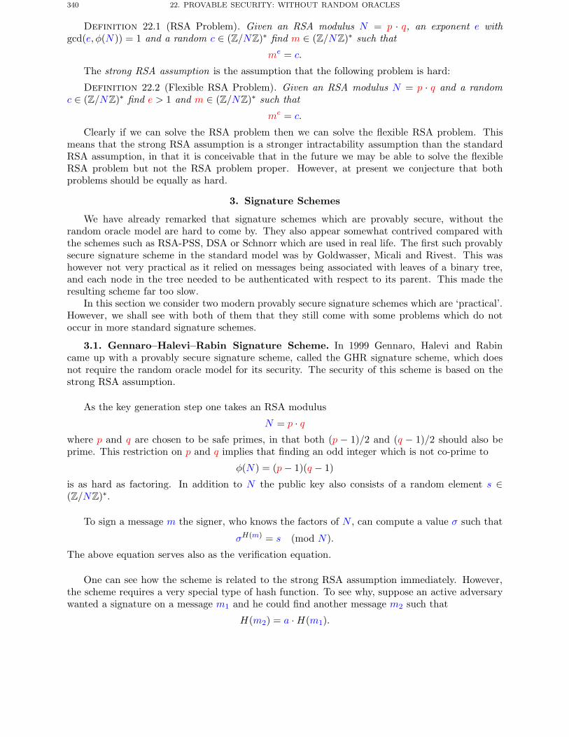
340 22. PROVABLE SECURITY: WITHOUT RANDOM ORACLES
Definition 22.1 (RSA Problem). Given an RSA modulus N = p · q, an exponent e withgcd(e, φ(N )) = 1 and a random c ∈ (Z/NZ)∗ find m ∈ (Z/NZ)∗ such that
me = c.
The strong RSA assumption is the assumption that the following problem is hard:
Definition 22.2 (Flexible RSA Problem). Given an RSA modulus N = p · q and a randomc ∈ (Z/NZ)∗ find e > 1 and m ∈ (Z/NZ)∗ such that
me = c.
Clearly if we can solve the RSA problem then we can solve the flexible RSA problem. Thismeans that the strong RSA assumption is a stronger intractability assumption than the standardRSA assumption, in that it is conceivable that in the future we may be able to solve the flexibleRSA problem but not the RSA problem proper. However, at present we conjecture that bothproblems should be equally as hard.
3. Signature Schemes
We have already remarked that signature schemes which are provably secure, without therandom oracle model are hard to come by. They also appear somewhat contrived compared withthe schemes such as RSA-PSS, DSA or Schnorr which are used in real life. The first such provablysecure signature scheme in the standard model was by Goldwasser, Micali and Rivest. This washowever not very practical as it relied on messages being associated with leaves of a binary tree,and each node in the tree needed to be authenticated with respect to its parent. This made theresulting scheme far too slow.
In this section we consider two modern provably secure signature schemes which are ‘practical’.However, we shall see with both of them that they still come with some problems which do notoccur in more standard signature schemes.
3.1. Gennaro–Halevi–Rabin Signature Scheme. In 1999 Gennaro, Halevi and Rabincame up with a provably secure signature scheme, called the GHR signature scheme, which doesnot require the random oracle model for its security. The security of this scheme is based on thestrong RSA assumption.
As the key generation step one takes an RSA modulus
N = p · qwhere p and q are chosen to be safe primes, in that both (p − 1)/2 and (q − 1)/2 should also beprime. This restriction on p and q implies that finding an odd integer which is not co-prime to
φ(N ) = (p − 1)(q − 1)
is as hard as factoring. In addition to N the public key also consists of a random element s ∈(Z/NZ)∗.
To sign a message m the signer, who knows the factors of N , can compute a value σ such that
σH(m) = s (mod N).
The above equation serves also as the verification equation.
One can see how the scheme is related to the strong RSA assumption immediately. However,the scheme requires a very special type of hash function. To see why, suppose an active adversarywanted a signature on a message m1 and he could find another message m2 such that
H(m2) = a ·H(m1).
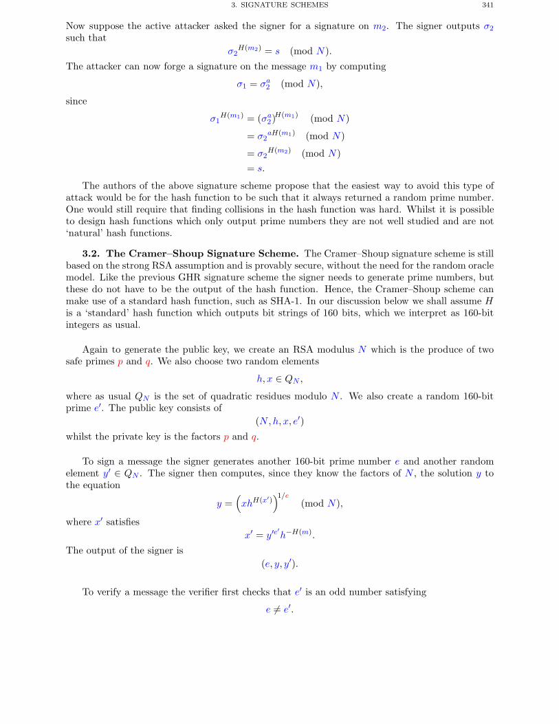
3. SIGNATURE SCHEMES 341
Now suppose the active attacker asked the signer for a signature on m2. The signer outputs σ2
such thatσ2H(m2) = s (mod N).
The attacker can now forge a signature on the message m1 by computing
σ1 = σa2 (mod N),
since
σ1H(m1) = (σa2)H(m1) (mod N)
= σ2aH(m1) (mod N)
= σ2H(m2) (mod N)
= s.
The authors of the above signature scheme propose that the easiest way to avoid this type ofattack would be for the hash function to be such that it always returned a random prime number.One would still require that finding collisions in the hash function was hard. Whilst it is possibleto design hash functions which only output prime numbers they are not well studied and are not‘natural’ hash functions.
3.2. The Cramer–Shoup Signature Scheme. The Cramer–Shoup signature scheme is stillbased on the strong RSA assumption and is provably secure, without the need for the random oraclemodel. Like the previous GHR signature scheme the signer needs to generate prime numbers, butthese do not have to be the output of the hash function. Hence, the Cramer–Shoup scheme canmake use of a standard hash function, such as SHA-1. In our discussion below we shall assume His a ‘standard’ hash function which outputs bit strings of 160 bits, which we interpret as 160-bitintegers as usual.
Again to generate the public key, we create an RSA modulus N which is the produce of twosafe primes p and q. We also choose two random elements
h, x ∈ QN ,
where as usual QN is the set of quadratic residues modulo N . We also create a random 160-bitprime e′. The public key consists of
(N,h, x, e′)whilst the private key is the factors p and q.
To sign a message the signer generates another 160-bit prime number e and another randomelement y′ ∈ QN . The signer then computes, since they know the factors of N , the solution y tothe equation
y =(xhH(x′)
)1/e(mod N),
where x′ satisfiesx′ = y′e
′h−H(m).
The output of the signer is(e, y, y′).
To verify a message the verifier first checks that e′ is an odd number satisfying
e �= e′.
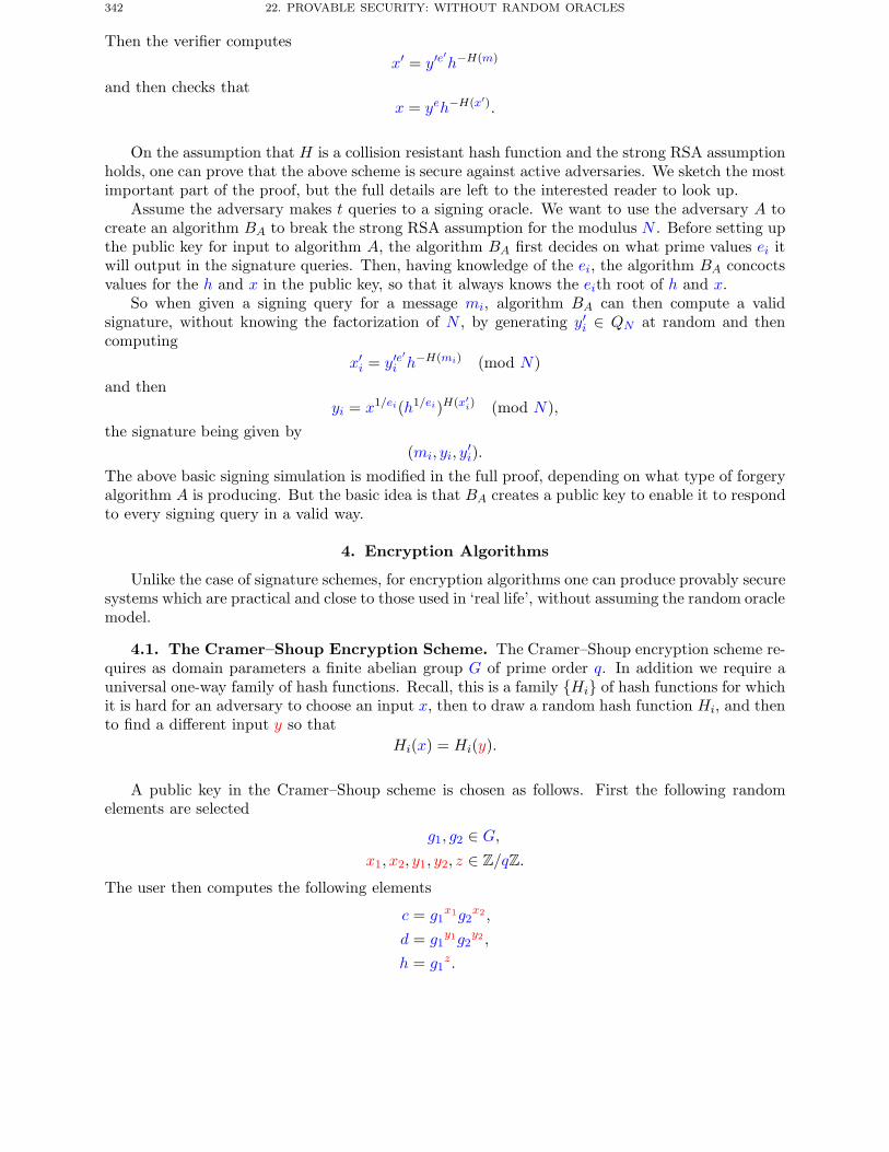
342 22. PROVABLE SECURITY: WITHOUT RANDOM ORACLES
Then the verifier computesx′ = y′e
′h−H(m)
and then checks thatx = yeh−H(x′).
On the assumption that H is a collision resistant hash function and the strong RSA assumptionholds, one can prove that the above scheme is secure against active adversaries. We sketch the mostimportant part of the proof, but the full details are left to the interested reader to look up.
Assume the adversary makes t queries to a signing oracle. We want to use the adversary A tocreate an algorithm BA to break the strong RSA assumption for the modulus N . Before setting upthe public key for input to algorithm A, the algorithm BA first decides on what prime values ei itwill output in the signature queries. Then, having knowledge of the ei, the algorithm BA concoctsvalues for the h and x in the public key, so that it always knows the eith root of h and x.
So when given a signing query for a message mi, algorithm BA can then compute a validsignature, without knowing the factorization of N , by generating y′i ∈ QN at random and thencomputing
x′i = y′e′
i h−H(mi) (mod N)
and thenyi = x1/ei(h1/ei)H(x′i) (mod N),
the signature being given by(mi, yi, y
′i).
The above basic signing simulation is modified in the full proof, depending on what type of forgeryalgorithm A is producing. But the basic idea is that BA creates a public key to enable it to respondto every signing query in a valid way.
4. Encryption Algorithms
Unlike the case of signature schemes, for encryption algorithms one can produce provably securesystems which are practical and close to those used in ‘real life’, without assuming the random oraclemodel.
4.1. The Cramer–Shoup Encryption Scheme. The Cramer–Shoup encryption scheme re-quires as domain parameters a finite abelian group G of prime order q. In addition we require auniversal one-way family of hash functions. Recall, this is a family {Hi} of hash functions for whichit is hard for an adversary to choose an input x, then to draw a random hash function Hi, and thento find a different input y so that
Hi(x) = Hi(y).
A public key in the Cramer–Shoup scheme is chosen as follows. First the following randomelements are selected
g1, g2 ∈ G,
x1, x2, y1, y2, z ∈ Z/qZ.
The user then computes the following elements
c = g1x1g2
x2,
d = g1y1g2
y2 ,
h = g1z.
4. ENCRYPTION ALGORITHMS 343
The user finally chooses a hash function H from the universal one-way family of hash functionsand outputs the public key
(g1, g2, c, d, h,H),whilst keeping the private key secret
(x1, x2, y1, y2, z).
The encryption algorithm proceeds as follows, which is very similar to ElGamal encryption.The message m is considered as an element of G. The sender then chooses a random ephemeralkey r ∈ Z/qZ and computes
u1 = g1r,
u2 = g2r,
e = m · hr,α = H(u1‖u2‖e),v = crdrα.
The ciphertext is then the quadruple(u1, u2, e, v).
On receiving this ciphertext the owner of the private key can recover the message as follows:First they compute α = H(u1‖u2‖e) and test whether
u1x1+y1αu2
x2+y2α = v.
If this equation does not hold then the ciphertext should be rejected. If this equation holds thenthe receiver can decrypt the ciphertext by computing
m =e
u1z.
To show that the scheme is provably secure, under the assumption that the DDH problem ishard and that H is chosen from a universal one-way family of hash functions, we assume we havean adversary A against the scheme and show how to use A in another algorithm BA which tries tosolve the DDH problem.
One way to phrase the DDH problem is as follows: Given (g1, g2, u1, u2) ∈ G determine whethereither this quadruple is a random quadruple or we have u1 = g1
r and u2 = g2r for some value of
r ∈ Z/qZ. So algorithm BA will take as input a quadruple (g1, g2, u1, u2) ∈ G and try to determinewhether this is a random quadruple or a quadruple related to the Diffie–Hellman problem.
Algorithm BA first needs to choose a public key, which it does in a non-standard way, by firstselecting the random elements
x1, x2, y1, y2, z1, z2 ∈ Z/qZ.
Algorithm BA then computes the following elements
c = g1x1g2
x2,
d = g1y1g2
y2 ,
h = g1z1g2
z2 .
Finally BA chooses a hash function H from the universal one-way family of hash functions andoutputs the public key
(g1, g2, c, d, h,H).
344 22. PROVABLE SECURITY: WITHOUT RANDOM ORACLES
Notice that the part of the public key corresponding to h has been chosen differently than in thereal scheme, but that algorithm A will not be able to detect this change.
Algorithm BA now runs the find stage of algorithm A, responding to decryption queries of(u′1, u′2, e′, v′) by computing
m =e′
u1′z1u′2z2
,
after performing the standard check on validity of the ciphertext. The output of the find stage willbe two plaintexts m0,m1.
After running the find stage, algorithm BA chooses a bit b at random and computes the targetciphertext as
e = mb · (u1z1u2
z2) ,
α = H(u1‖u2‖e),v = u1
x1+y1αu2x2+y2α.
The target ciphertext is then the quadruple
(u1, u2, e, v).
Notice that when the input to BA is a legitimate DDH quadruple then the target ciphertext will bea valid encryption, but when the input to BA is not a legitimate DDH quadruple then the targetciphertext is highly likely to be an invalid ciphertext.
This target ciphertext is then passed to the guess stage of the adversary A. If this adversaryoutputs the correct value of b then we suspect that the input to BA is a valid DDH quadruple,whilst if the output is wrong then we suspect that the input to BA is not valid. This produces astatistical test to detect whether the input to BA was valid or not. By repeating this test a numberof times we can produce as accurate a statistical test as we want.
Note, that the above is only a sketch. We need to show that the view of the adversary A inthe above game is no different from that in a real attack on the system, otherwise A would knowsomething was not correct. For example we need to show that the responses BA makes to thedecryption queries of A cannot be distinguished from a true decryption oracle. For further detailsone should consult the full proof in the paper mentioned in the Further Reading section.
Notice that, whilst very similar to ElGamal encryption, the Cramer–Shoup encryption schemeis much less efficient. Hence, whilst provably secure it is not used much in practice due to theperformance disadvantages.
Chapter Summary
• Signature schemes which are secure without the random oracle model are less natural thanthose which are secure in the random oracle model. This is probably because signaturesmake crucial use of hash functions which are easy to model by random oracles.
• The strong RSA assumption is a natural weakening of the standard RSA assumption.• The Cramer–Shoup encryption scheme is provably secure, without the random oracle
model, assuming the DDH problem is hard. It is around three times slower than the usualElGamal encryption algorithm.
Further Reading 345
Further Reading
The schemes mentioned in this chapter can be found in the following papers.
M. Abdalla, M. Bellare and P. Rogaway. DHAES: An encryption scheme based on the Diffie–Hellman problem. Submission to IEEE P1363a standard.
R. Cramer and V. Shoup. A practical public key cryptosystem provably secure against adaptivechosen ciphertext attack. In Advances in Cryptology – CRYPTO ’98, Springer-Verlag LNCS 1462,13–25, 1998.
R. Cramer and V. Shoup. Signature schemes based on the strong RSA assumption. ACM Transac-tions on Information and Systems Security, 3, 161–185, 2000.
R. Gennaro, S. Halevi and T. Rabin. Secure hash-and-sign signatures without the random oracle.In Advances in Cryptology – EuroCrypt ’99, Springer-Verlag LNCS 1592, 123–139, 1999.

Part 5
Advanced Protocols
Encryption, Hash Functions, MACs and Signatures are only the most basic of cryptographicconstructions and protocols. We usually think of them as being carried out between a sender anda receiver who have the same security goals. For example in encryption, both the sender and thereceiver probably wish to keep the message secret from an adversary. In other words the adversaryis assumed to be someone else.
In this section we shall detail a number of more advanced protocols. These are mainly protocolsbetween two or more people, in which the security goals of the different parties could be conflicting,or different. For example in an electronic election voters want their votes to be secret, yet all partieswant to know that all votes have been counted, and all parties want to ensure against a bad votercasting too many votes. Hence, the adversaries are also the parties in the protocol, they are notnecessarily external entities.
First we focus on secret sharing schemes, which allow a party to share a secret amongst a numberof partners. This has important applications in splitting of secrets into parts which can then be usedin distributed protocols. Then we turn to commitments schemes and oblivious transfer. These aretwo types of basic protocols between two parties, in which the parties are assumed to be mutuallyuntrustworthy, i.e. the adversary is the person who you are performing the protocol with. We thenturn to the concept of zero-knowledge proofs. In this chapter we also examine a simple electronicvoting scheme. Finally we look at the subject of secure multi-party computation, which providesan interesting application of many of our proceeding algorithms.

CHAPTER 23
Secret Sharing Schemes
Chapter Goals
• To introduce the notion of secret sharing schemes.• To give some simple examples for general access structures.• To present Shamir’s scheme, including how to recover the secret in the presence of active
adversaries.• To show the link between Shamir’s secret sharing and Reed–Solomon codes.
1. Introduction
Suppose you have a secret s which you wish to share amongst n parties P . You would likecertain subsets of the n parties to recover the secret but not others. The classic scenario mightbe that s is nuclear launch code and you have four people, the president, the vice-president, thesecretary of state and a general in a missile silo. You do not want the general to be able to launchthe missile without the president agreeing, but to maintain deterrence you would like, in the casethe president has been eliminated, that the vice-president, the secretary of state and the generalcan agree to launch the missile. If we label the four parties as P, V, S and G, for president, vice-president, secretary of state and general, then we would like the following sets of people to be ableto launch the missile
{P,G} and {V, S,G},but no smaller sets. It is this problem which secret sharing is designed to deal with, however theapplications are more widespread than might at first appear.
To each party we distribute some information called the share. For a party A we will let sAdenote the secret share which they hold. In the example above there are four such shares sP , sV ,sS and sG. Then if the required parties come together we would like an algorithm which combinestheir relevant shares into the secret s. It is this problem which this chapter addresses.
2. Access Structures
Before introducing schemes to perform secret sharing we first however, need to introduce thenotion of an access structure. Any subset of parties who can recover the secret will be called aqualifying set, whilst the set of all qualifying sets will be called an access structure. So in theexample above we have that the two sets
{P,G} and {V, S,G}are qualifying sets. However, clearly any set containing such a qualifying set is also a qualifyingset. Thus
{P,G, V }, {P,G, S} and {P, V,G, S}are also qualifying sets. Hence, there are five sets in the access structure. For any set in the accessstructure, if we have the set of shares for that set we would like to be able to reconstruct the secret.
349
350 23. SECRET SHARING SCHEMES
Definition 23.1. Consider a set P. A monotone structure on P is a collection Γ of subsets ofP such that
• P ∈ Γ• If A ∈ Γ and B is a set such that A ⊂ B ⊂ P then B ∈ Γ.
Thus in the above example the access structure is monotone. This is a property which will holdfor all access structures of all secret sharing schemes. For a monotone structure we note that thesets in Γ come in chains, A ⊂ B ⊂ C ⊂ P. We shall call the sets which form the start of a chain,the minimal qualifying sets. The set of all such minimal qualifying sets for an access structure Γwe shall denote by m(Γ). We can now give a very informal definition of what we mean by a secretsharing scheme:
Definition 23.2. A secret sharing scheme for a monotone access structure Γ over a set ofparties P with respect to a space of secrets S, is a pair of algorithms called Share and Recombinewith the following properties:
• Share(s,Γ) takes a secret s and a monotone access structure and determines a value sAfor every A ∈ P. The value sA is called A’s share of the secret.
• Recombine(H) takes a set H of shares for some set O of P, i.e.
H = {sO : O ∈ O}.If O ∈ Γ then this should return the secret s, otherwise it should return nothing.
A secret sharing scheme is considered to be secure if no adversary can learn anything about theunderlying secret without having access to the shares of a qualifying set. Actually such schemes aresaid to be information theoretically secure, but since most secret sharing schemes in the literatureare information theoretically secure we shall just call such schemes secure.
In this chapter we will consider two running examples of monotone access structures, so as toillustrate the schemes. Both will be on sets of four elements: The first is from the example abovewhere we have P = {P, V, S,G} and
Γ = {{P,G}, {V, S,G}, {P,G, V }, {P,G, S}, {P, V,G, S}} .The set of minimal qualify sets are given by
{{P,G}, {V, S,G}} .The second example we shall define over the set of parties P = {A,B,C,D}, with access structure
Γ = {{A,B}, {A,C}, {A,D}, {B,C}, {B,D}, {C,D},{A,B,C}, {A,B,D}, {B,C,D}, {A,B,C,D} } .
The set of minimal qualify sets are given by
{{A,B}, {A,C}, {A,D}, {B,C}, {B,D}, {C,D}} .This last access structure is interesting because it represents a common structure of a thresholdaccess structure. Notice that we require that any two out of the four parties should be able torecover the secret. We call such a scheme a 2-out-of-4 threshold access structure.
One way of looking at such access structures is via a boolean formulae. Consider the set m(Γ)of minimal qualifying sets and define the formulae:
∨O∈m(Γ)
( ∧O∈O
O
).
3. GENERAL SECRET SHARING 351
For example in our first example above the formulae becomes
(P ∧G) ∨ (V ∧ S ∧G).
Reading this formulae out, with ∧ being “and”, and ∨ being “or”, we see that one can reconstructthe secret if we have access to the secret shares of
(P and G) or (V and S and G).
Notice how the formula is in disjunctive normal form (DNF).
3. General Secret Sharing
We now turn to two methods for constructing secret sharing schemes for arbitrary monotoneaccess structures. They are highly inefficient for all but the simplest access structures but they doshow that one can cope with an arbitrary access structure. We assume that the space of secrets Sis essentially the set of bit strings of length n-bits. In both examples we let s ∈ S denote the secretwhich we are trying to share.
3.1. Ito-Nishizeki-Saito Secret Sharing. Our first secret sharing scheme makes use ofthe DNF boolean formulae we presented above. In some sense every “or” gets converted into aconcatenation operation and every “and” gets converted into a ⊕ operation, note this can at firstsight seem slightly counter-intuitive.
The sharing algorithm works as follows. For every minimal qualifying set O ∈ m(Γ), we generateshares si ∈ S, for 1 ≤ i ≤ l, at random, where l = |O| such that s1 ⊕ · · · ⊕ sl = s. Then a party Ais given a share si if it occurs as position i in the set O.
3.1.1. Example 1: Recall we have the formulae
(P and G) or (V and S and G).
We generate shares five elements si from S such that
s = s1 ⊕ s2,
= s3 ⊕ s4 ⊕ s5.
The four shares are then defined to be:
sP = s1,
sV = s3,
sS = s4,
sG = s2‖s5.
You should check that, given this sharing, any qualifying set can recover the secret, and only thequalifying sets can recover the secret. Notice, that party G needs to hold two times more datathan the size of the secret. Thus this scheme in this case is not efficient. Ideally we would like theparties to only hold the equivalent of n bits of information each so as to recover a secret of n bits.
3.1.2. Example 2: Now our formulae is given by.
(A and B) or (A and C) or (A and D) or (B and C) or (B and D) or (C and D).
352 23. SECRET SHARING SCHEMES
We now generate shares for twelve elements si from S, one for each of the distinct terms in theformulae above, such that
s = s1 ⊕ s2,
= s3 ⊕ s4,
= s5 ⊕ s6,
= s7 ⊕ s8,
= s9 ⊕ s10,
= s11 ⊕ s12.
The four shares are then defined to be:
sA = s1‖s3‖s5,sB = s2‖s7‖s9,sC = s4‖s8‖s11,sD = s6‖s10‖s12.
You should again check that, given this sharing, any qualifying set and only the qualifying sets canrecover the secret. We see that in this case every share contains three times more information thanthe underlying secret.
3.2. Replicated Secret Sharing. The above is not the only scheme for general access struc-ture. Here we present another one called the replicated secret sharing scheme. In this scheme wefirst create the sets of all maximal non-qualifying sets, these are the sets of all parties such thatif you add a single new party to each set you will obtain a qualifying set. If we label these setsA1, . . . , At, we then form their set-theoretic complements, i.e. Bi = P \ Ai. A set of secret sharessi is then generated, one for each set Bi, so that
s = s1 ⊕ · · · ⊕ st.
Then a party is given the share si if it is contained in the set Bi.
3.2.1. Example 1: The sets of maximal non-qualifying sets for this example are
A1 = {P, V, S}, A2 = {V,G} and A3 = {S,G}Forming their complements we obtain the sets
B1 = {G}, B2 = {P, S} and B3 = {P, V }.We generate three shares s1, s2 and s3 such that s = s1 ⊕ s2 ⊕ s3 and then define the shares as
sP = s2‖s3,sV = s3,
sS = s2,
sG = s1.
Again we can check that only the qualifying sets can recover the secret.
4. REED–SOLOMON CODES 353
3.2.2. Example 2: For the 2-out-of-4 threshold access structure we obtain the following maximalnon-qualifying sets
A1 = {A}, A2 = {B}, A3 = {C} and A4 = {D}.On forming their complements we obtain
B1 = {B,C,D}, B2 = {A,C,D}, B3 = {A,B,D} and B4 = {A,B,C}.We form the four shares such that s = s1 ⊕ s2 ⊕ s3 ⊕ s4 and
sA = s2‖s3‖s4,sB = s1‖s3‖s4,sC = s1‖s2‖s4,sD = s1‖s2‖s3.
Whilst the above two constructions provide a mechanism to construct a secret sharing schemefor any monotone access structure, they appear to be very inefficient. In particular for the thresholdaccess structure they are particularly bad, especially as the number of parties increases. In the restof this chapter we will examine a very efficient mechanism for threshold secret sharing due toShamir, called Shamir secret sharing. This secret sharing scheme is itself based on the ideas behindcertain error-correcting codes, called Reed–Solomon codes. So we will first have a little digressioninto coding theory.
4. Reed–Solomon Codes
An error-correcting code is a mechanism to transmit data from A to B such that any errors whichoccur during transmission, for example due to noise, can be corrected. They are found in manyareas of electronics; they are the thing which makes your CD/DVD resistant to minor scratches,they make sure that RAM chips preserve your data correctly, they are used for communicationbetween earth and satellites or deep space probes.
A simpler problem is one of error-detecting. Here one is only interested in whether the data hasbeen altered or not. A particularly important distinction to make between the area of coding theoryand cryptography is that in coding theory one can select simpler mechanisms to detect errors. Thisis because, in coding theory the assumption is that the errors are introduced by random noise,whereas in cryptography any errors are thought to be actively inserted by an adversary. Thus incoding theory, error detection mechanisms can be very simple, whereas in cryptography we haveto resort to complex mechanism’s such as MAC’s and digital signatures.
Error correction on the other hand is not only interested with detecting errors, it also wants tocorrect those errors. Clearly one cannot correct all errors, but it would be nice to correct a certainnumber. A classic way of forming error-correcting codes is via Reed–Solomon codes. Usually suchcodes are presented, in coding theory, over a finite field of characteristic two. However, we areinterested in the general case and so we will be using a code over Fq, for a prime power q.
To define a Reed–Solomon code we also require two other integer parameters n and t. Thevalue n defines the length of each code-word, whilst the number t is related to the number of errorswe can correct. We also define a set X ⊂ Fq of size n. If the characteristic of Fq is larger thann then we can select X = {1, 2, . . . , n}, although any set will do. For our application to Shamirsecret sharing later on we will assume that 0 �∈ X .
Consider the set of polynomials of degree less than or equal to t over the field Fq.
P ={f0 + f1X + . . .+ ftX
t : fi ∈ Fq}.
The set P represents the total number of code-words in our code, i.e. the amount of different datawhich we can transmit in any given block. The total number of code-words is then equal to qt+1.
354 23. SECRET SHARING SCHEMES
To create the actual code-word we evaluate the polynomial at all elements in X . Hence, the set ofactual code-words is given by
C = {(f(x1), . . . , f(xn)) : f ∈ P, xi ∈ X} .The length of a code word is then given by n · log2 q. So we require n · log2 q bits to represent(t+ 1) · log2 q bits of information.
As an example consider the Reed–Solomon code with parameters q = 101, n = 7, t = 2 andX = {1, 2, 3, 4, 5, 6, 7}. Suppose our “data”, which is represented by an element of P, is given bythe polynomial
f = 20 + 57X + 68X2.
To transmit this data we compute f(i) (mod q) for i = 1, . . . , 7, to obtain the code-word
c = (44, 2, 96, 23, 86, 83, 14).
This code-word can now be transmitted or stored.
4.1. Data Recovery. At some point the code-word will need to be converted back into thedata. In other words we have to recover the polynomial in P from the set of points at which it wasevaluated, i.e. the vector of values in C. We will first deal with the simple case and assume thatno errors have occurred.
The receiver is given the data c = (c1, . . . , cn) but has no idea as to the underlying polynomialf . Thus from the receivers perspective he wishes to find the fi such that
f =t∑
j=0
fjXj .
It is well known, from high school, that a polynomial of degree at most t is determined completelyby its values at t+1 points. So as long as t < n we can recover f when no errors occur; the questionis how?
First note that the receiver can generate n linear equations via
ci = f(xi) for xi ∈ X.In other words he has the system of equations:
c1 = f0 + f1x1 + · · · + ftxt1,
......
cn = f0 + f1x1 + · · · + ftxtn.
So by solving this system of equations over the field Fq we can recover the polynomial and hencethe data.
Actually the polynomial f can be recovered without the need for solving the linear system, viathe use of Lagrange interpolation. Suppose we first compute the polynomials
δi(X) =∏
xj∈X,j �=i
X − xjxi − xj
, 1 ≤ i ≤ n.
Note that we have the following properties, for all i.
• δi(xi) = 1.• δi(xj) = 0, if i �= j.• deg δi(X) = n− 1.
4. REED–SOLOMON CODES 355
Lagrange interpolation takes the values ci and computes
f(X) =n∑i=1
ci · δi(X).
The three properties above on the polynomials δi(X) translate into the following facts above f(X)• f(xi) = ci for all i.• deg f(X) ≤ n− 1.
Hence, Lagrange interpolation finds the unique polynomial which interpolates the n elements inthe code-word.
4.2. Error Detection. Returning to our Reed–Solomon codes we see that by using Lagrangeinterpolation on the code-word we will recover a polynomial of degree t when their are no errors,but when there are errors in the received code-word we are unlikely to obtain a valid polynomial,i.e. an element of P. Hence, we instantly have an error-detection algorithm.
Returning to our example parameters above. Suppose the following code-word was received
c = (44, 2, 25, 23, 86, 83, 14).
In other words it is equal to the sent code-word except in the third position where a 96 has beenreplaced by a 25. We compute once and for all the polynomials, modulo q = 101,
δ1(X) = 70X6 + 29X5 + 46X4 + 4X3 + 43X2 + 4X + 7,
δ2(X) = 85X6 + 12X5 + 23X4 + 96X3 + 59X2 + 49X + 80,
δ3(X) = 40X6 + 10X5 + 83X4 + 23X3 + 48X2 + 64X + 35,
δ4(X) = 14X6 + 68X5 + 33X4 + 63X3 + 78X2 + 82X + 66,
δ5(X) = 40X6 + 90X5 + 99X4 + 67X3 + 11X2 + 76X + 21,
δ6(X) = 85X6 + 49X5 + 91X4 + 91X3 + 9X2 + 86X + 94,
δ7(X) = 70X6 + 45X5 + 29X4 + 60X3 + 55X2 + 43X + 1.
The receiver now tries to recover the sent polynomial given the data he has received. He obtains
f(X) = 44 · δ1(X) + · · · + 14 · δ7(X) = 60 + 58X + 94X2 + 84X3 + 66X4 + 98X5 + 89X6.
But this is a polynomial of degree six and not of degree t = 2. Hence, the receiver knows that thereis at least one error in the code word that he has received. He just does not know which one is inerror, nor what its actual value should be.
4.3. Error Correction. The intuition behind error correction is the following. Consider apolynomial of degree three over the reals evaluates in seven points, such as that in Figure 1.Clearly there is only one cubic curve which interpolates all of the points, since we have specifiedseven of them and we only need four such points to define a cubic curve. Now suppose one of theseevaluations is given in error, for example the point at x = 3, as in Figure 2. We see that we stillhave six points on the cubic curve, and so there is a unique cubic curve passing through these sixvalid points. However, if we took another six points, i.e. five valid ones and the error one, then itis highly likely that the curve which goes through second six points would not be cubic.
In other words because we have far more valid points than we need to determine the cubic curve,we are able to recover it. This leads to a very inefficient method for polynomial reconstruction.We return to the general case of a polynomial of degree t evaluated at n points. Suppose we knowthat there are at most e errors in our code-word. Then we simply produce the list of all subsetsS of the n points with n− e members. We then try to recover a polynomial of degree t, if we aresuccessful then we have a good probability that the subset S is the valid set, if we are unsuccessfulthen we know that S contains an element which is in error.
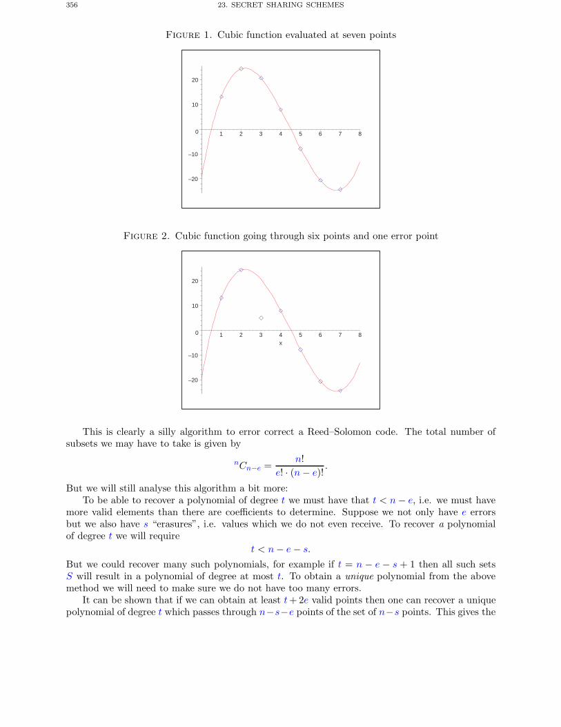
356 23. SECRET SHARING SCHEMES
Figure 1. Cubic function evaluated at seven points
–20
–10
0
10
20
1 2 3 4 5 6 7 8
Figure 2. Cubic function going through six points and one error point
–20
–10
0
10
20
1 2 3 4 5 6 7 8x
This is clearly a silly algorithm to error correct a Reed–Solomon code. The total number ofsubsets we may have to take is given by
nCn−e =n!
e! · (n− e)!.
But we will still analyse this algorithm a bit more:To be able to recover a polynomial of degree t we must have that t < n− e, i.e. we must have
more valid elements than there are coefficients to determine. Suppose we not only have e errorsbut we also have s “erasures”, i.e. values which we do not even receive. To recover a polynomialof degree t we will require
t < n− e− s.
But we could recover many such polynomials, for example if t = n − e − s + 1 then all such setsS will result in a polynomial of degree at most t. To obtain a unique polynomial from the abovemethod we will need to make sure we do not have too many errors.
It can be shown that if we can obtain at least t+ 2e valid points then one can recover a uniquepolynomial of degree t which passes through n−s−e points of the set of n−s points. This gives the
4. REED–SOLOMON CODES 357
important equation that an error correction for Reed–Solomon codes can be performed uniquelyprovided
n > t+ 2e+ s.
The only problem left is how to perform this error correction efficiently.
4.4. The Berlekamp–Welch Algorithm. We now present an efficient method to performerror correction for Reed–Solomon codes called the Berlekamp–Welch algorithm. The idea is tointerpolate a polynomial in two variables through the points which we are given. Suppose we aregiven a code word with s missing values, and the number of errors is bounded by
e < t <n− s
3.
This means we are actually given n − s supposed values of yi = f(xi). We know the pairs (xi, yi)and we know that at most e of them are wrong, in that they do not come from evaluating thehidden polynomial f(X). The goal of error correction is to try to recover this hidden polynomial.
We first construct the bivariate polynomial
Q(X,Y ) = f0(X) − f1(X) · Y,where f0 (resp. f1) is a polynomial of degree at most 2 · t (resp. t). We impose the condition thatf1(0) = 1. We treat the coefficients of the fi as variables which we want to determine. Due to thebounds on the degrees of the two polynomials, and the extra condition of f1(0) = 1, we see thatthe number of variables we have is
v = (2 · t+ 1) + (t+ 1) − 1 = 3 · t+ 1.
We would like the bivariate polynomial Q(X,Y ) to interpolate our points (xi, yi). By substitutingin the values of xi and yi we obtain a linear equation in terms of the unknown coefficients of thepolynomials fi. Since we have n− s such points, the number of linear equations we obtain is n− s.
After determining f0 and f1 we then compute
f =f0
f1.
To see this consider the single polynomial in one variable
P (X) = Q(X, f(X))
where f(X) is the polynomial we are trying to determine. We have degP (X) ≤ 2t. The polynomialP (X) clearly has at least n− s− e zero’s, i.e. the number of valid pairs. So the number of zeros isat least
n− s− e > n− e− t > 3t− t = 2t,since e < t < n−s
3 . Thus P (X) has more zeros than it’s degree, and it must hence be the zeropolynomial. Hence,
f0 − f1 · f = 0and so f = f0/f1 since f1 �= 0.
Again consider our previous example, we have received the invalid code-word
c = (44, 2, 25, 23, 86, 83, 14).
We know that the underlying code is for polynomials of degree t = 2. Hence, since 2 = t < n−s3 =
7/3 = 2.3 we should be able to correct a single error. Using the method above we want to determinethe polynomial Q(X,Y ) of the form
Q(X,Y ) = f0,0 + f1,0X + f2,0X2 + f3,0X
3 + f4,0X4 − (1 + f1,1X + f2,1X
2)Y
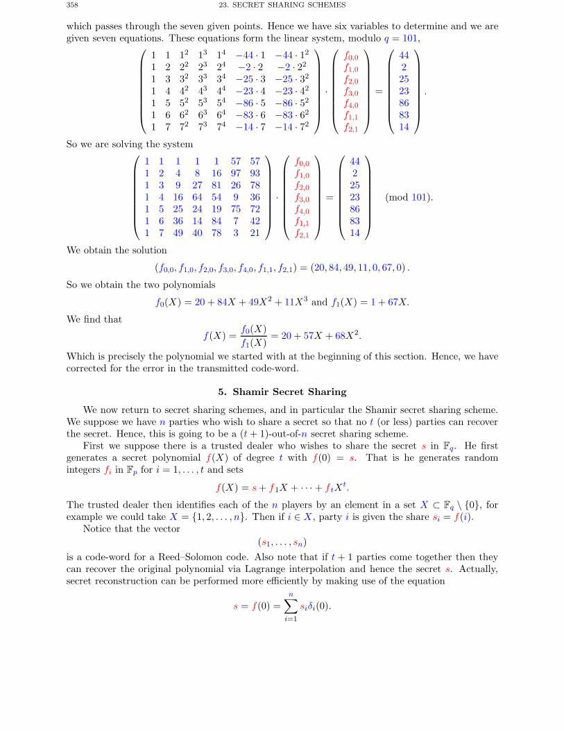
358 23. SECRET SHARING SCHEMES
which passes through the seven given points. Hence we have six variables to determine and we aregiven seven equations. These equations form the linear system, modulo q = 101,⎛
⎜⎜⎜⎜⎜⎜⎜⎜⎝
1 1 12 13 14 −44 · 1 −44 · 12
1 2 22 23 24 −2 · 2 −2 · 22
1 3 32 33 34 −25 · 3 −25 · 32
1 4 42 43 44 −23 · 4 −23 · 42
1 5 52 53 54 −86 · 5 −86 · 52
1 6 62 63 64 −83 · 6 −83 · 62
1 7 72 73 74 −14 · 7 −14 · 72
⎞⎟⎟⎟⎟⎟⎟⎟⎟⎠
·
⎛⎜⎜⎜⎜⎜⎜⎜⎜⎝
f0,0
f1,0
f2,0
f3,0
f4,0
f1,1
f2,1
⎞⎟⎟⎟⎟⎟⎟⎟⎟⎠
=
⎛⎜⎜⎜⎜⎜⎜⎜⎜⎝
4422523868314
⎞⎟⎟⎟⎟⎟⎟⎟⎟⎠.
So we are solving the system⎛⎜⎜⎜⎜⎜⎜⎜⎜⎝
1 1 1 1 1 57 571 2 4 8 16 97 931 3 9 27 81 26 781 4 16 64 54 9 361 5 25 24 19 75 721 6 36 14 84 7 421 7 49 40 78 3 21
⎞⎟⎟⎟⎟⎟⎟⎟⎟⎠
·
⎛⎜⎜⎜⎜⎜⎜⎜⎜⎝
f0,0
f1,0
f2,0
f3,0
f4,0
f1,1
f2,1
⎞⎟⎟⎟⎟⎟⎟⎟⎟⎠
=
⎛⎜⎜⎜⎜⎜⎜⎜⎜⎝
4422523868314
⎞⎟⎟⎟⎟⎟⎟⎟⎟⎠
(mod 101).
We obtain the solution
(f0,0, f1,0, f2,0, f3,0, f4,0, f1,1, f2,1) = (20, 84, 49, 11, 0, 67, 0) .
So we obtain the two polynomials
f0(X) = 20 + 84X + 49X2 + 11X3 and f1(X) = 1 + 67X.
We find that
f(X) =f0(X)f1(X)
= 20 + 57X + 68X2.
Which is precisely the polynomial we started with at the beginning of this section. Hence, we havecorrected for the error in the transmitted code-word.
5. Shamir Secret Sharing
We now return to secret sharing schemes, and in particular the Shamir secret sharing scheme.We suppose we have n parties who wish to share a secret so that no t (or less) parties can recoverthe secret. Hence, this is going to be a (t+ 1)-out-of-n secret sharing scheme.
First we suppose there is a trusted dealer who wishes to share the secret s in Fq. He firstgenerates a secret polynomial f(X) of degree t with f(0) = s. That is he generates randomintegers fi in Fp for i = 1, . . . , t and sets
f(X) = s+ f1X + · · · + f tXt.
The trusted dealer then identifies each of the n players by an element in a set X ⊂ Fq \ {0}, forexample we could take X = {1, 2, . . . , n}. Then if i ∈ X, party i is given the share si = f(i).
Notice that the vector(s1, . . . , sn)
is a code-word for a Reed–Solomon code. Also note that if t + 1 parties come together then theycan recover the original polynomial via Lagrange interpolation and hence the secret s. Actually,secret reconstruction can be performed more efficiently by making use of the equation
s = f(0) =n∑i=1
siδi(0).
5. SHAMIR SECRET SHARING 359
Hence, if we define for a set Y ⊂ X the vector rY by rY = (rxi,Y , . . . , rxi,Y )xi∈Y to be the public“recombination” vector, where
rxi,Y =∏
xj∈Y ,xj �=xi
−xjxi − xj
.
Then, if we obtain a set of shares back from a subset Y ⊂ X with #Y > t, we can recover s viathe simple summation.
s =∑xi∈Y
rxi,Y · si.
Also note that if we receive from a set of parties Y some possible share values, then we canrecover the original secret via the Berlekamp–Welch algorithm for decoding Reed-Solomon code inthe presence of errors. Assuming the number of errors is bounded by e where
e < t <#Y3.
An interesting property of Shamir secret sharing is that we can do without the trusted dealercompletely, in the case when t = n − 1, i.e. the case when we want all parties to come togetherto recover the secret. Suppose we have n parties and they wish to share a secret, but it does notmatter what the secret actually is, only that it is shared in a n-out-of-n secret sharing scheme. Todo this they all simply generate a random integer si as their share. These will define a polynomialof degree n − 1, and the resulting polynomial will be able to be recovered when all parties cometogether.
Shamir secret sharing is also an example of a scheme which can be made into a pseudorandomsecret sharing scheme, or PRSS. This is a secret sharing scheme which allows the parties to generatea sharing of a random value with almost no interaction. For an n-out-of-n scheme this is simplesince each party only needs to generate a random value, and then the common shared secret valueis the sum of all the various shares. However, we wish to do this for a general (t + 1)-out-of-nscheme.
To create such a scheme for the Shamir secret sharing scheme requires some initial interactionto perform the setup, then the parties can generate as many shares of random values as they wish,with no further interaction. To define the Shamir pseudorandom secret sharing scheme we takeour n parties, labelled by the set X = {1, 2, . . . , n}, and threshold value t. Then for every subsetA ⊂ X of size n− t we define the polynomial fA(X) of degree t by the conditions
fA(0) = 1 and fA(i) = 0 for all i ∈ X \A.In the initialisation phase for our PRSS we create a secret value rA ∈ S, where S is some key space,for each subset A, this is securely distributed to each set A. The n parties also agree on a publicpseudorandom function which is keyed by the secret values rA,
ψ :{
S × S −→ Fq(rA, x) −→ ψ(rA, x).
Now when the parties wish to generate a new secret sharing of a random value. By some means,either by interaction or by prearrangement (e.g. a counter value), they select a public random valuea ∈ S. The underlying polynomial of degree t is given by
f(X) =∑
A⊂{1,...,n},|A|=n−tψ(rA, a) · fA(X),
where the sum is over all subsets A of size n− t. This means that each party i receives the share
si =∑
i∈A⊂{1,...,n},|A|=n−tψ(rA, a) · fA(i)
360 23. SECRET SHARING SCHEMES
where the sum is over all subsets A of size n− t which contain the element i. Finally the randomvalue which is shared, via the Shamir secret sharing scheme, is given by
s =∑
A⊂{1,...,n},|A|=n−tψ(rA, a) · fA(0) =
∑A⊂{1,...,n},|A|=n−t
ψ(rA, a).
In Chapter 26 we shall require not only pseudorandom secret sharing, but also a variant calledpseudorandom zero sharing, or PRZS, for the Shamir secret sharing scheme. In pseudorandomzero sharing we wish to generate random sharings of the value zero, with respect to a polynomialof degree 2 · t. For this we require exactly the set up as for the PRSS, but now we a differentpseudorandom function,
ψ :{S × S × {1, . . . , t} −→ Fq
(rA, x, j) −→ ψ(rA, x, j).
Then to create a degree 2 · t Shamir secret sharing of zero, the parties pick a number a as before.The underlying polynomial is then given by
f(X) =∑
A⊂{1,...,n},|A|=n−t
⎛⎝ t∑j=1
ψ(rA, a) ·Xj · fA(X)
⎞⎠ .
Clearly this is a polynomial which shares the zero value.
6. Application: Shared RSA Signature Generation
We shall now present a simple application of a secret sharing scheme, which has applicationsin the real world. Suppose a company is setting up a certificate authority to issue RSA signedcertificates to its employees to enable them to access various corporate services. It considers theassociated RSA private key to be highly sensitive, after all if the private key was compromised thenthe entire companies corporate infrastructure could also be compromised. Suppose the public keyis (N, e) and the private key is d.
The company decide that to mitigate the risk they will divide the private key into three sharesand place the three shares on three different continents. Thus, for example, there will be one serverin Asia, one in America and one in Europe. As soon as the RSA key is generated the companygenerates three integers d1, d2 and d3 such that
d = d1 + d2 + d3 (mod φ(N)).
The company then removes all knowledge of d and places d1 on a secure computer in Asia, d2 ona secure compute in America and d3 on a secure computer in Europe.
Now an employee wishes to obtain a digital certificate. This is essentially the RSA signatureon a (possibly hashed) string m. The employee simply sends the string m to the three computers,who respond with
si = mdi for i = 1, 2, 3.The valid RSA signature is then obtained by multiplying the three shares together, i.e
s = s1 · s2 · s3 = md1+d2+d3 = md.
This scheme appears to solve the problem of putting the master signature key in only one location.However, the employee now needs for the three servers to be online in order to obtain his certificate.It would be much nicer if only two had to be online, since then the company could cope with outagesof servers.
The problem is that the above scheme essentially implements a 3-out-of-3 secret sharing scheme,whereas what we want is a 2-out-of-3. Clearly, we need to apply something along the lines of Shamir
6. APPLICATION: SHARED RSA SIGNATURE GENERATION 361
secret sharing. However, the problem is that the number φ(N ) needs to be kept secret, and thedenominators in the Lagrange interpolation formulae may not be coprime to φ(N ).
There have been many solutions proposed to the above problem of threshold RSA, however, themost elegant and simple is due to Shoup. Suppose we want a t-out-of-n sharing of the RSA secretkey d, where we assume that e is chosen so that it is a prime and e > n. We adapt the Shamirscheme as follows: Firstly a polynomial of degree t − 1 is chosen, by selecting fi modulo φ(N) atrandom, to obtain
f(X) = d+ f1X + · · · + f t−1Xt−1.
Then each server is given the share di = f(i). The number of parties n is assumed to be fixed andwe set Δ = n!.
Now suppose a user wishes to obtain a signature on the message m, i.e it wants to compute md
(mod N). It sends m to each server, which then computes the signature fragment as
si = m2Δdi (mod N).
These signature fragments are then sent back to the user.Suppose now that the user obtains fragments back from a subset Y = {i1, . . . , it} ⊂ {1, . . . , n},
of size greater than or equal to t. Consider the “recombination” vector defined by
rij ,Y =∏
ik∈Y ,ij �=ik
−ikij − ik
.
We really want to be able to compute this modulo φ(N ) but that is impossible. However we notethat the denominator in the above divides Δ and so we have that Δ · rij ,Y ∈ Z. Hence, the usercan compute
s′ =∏ij∈Y
sij2·Δ·rij ,Y (mod N).
We find that this is equal to
s′ =(m4·Δ2
)Pij∈Y rij ,Y ·dij
= m4·Δ2·d (mod N).
With the last equality working due to Lagrange interpolation modulo φ(N). From this partialsignature we need to recover the real signature. To do this we use the fact that we have assumedthat e > n and e is a prime. These latter two facts mean that e is coprime to 4 ·Δ2, and so via theextended Euclidean algorithm we can compute integers u and v such that
u · e+ v · 4 · Δ2 = 1.
From which the signature is computed as
s = mu · s′v (mod N).
That s is the valid RSA signature for this public/private key pair can be verified since
se =(mu · s′v)e ,
= me·u ·m4·e·v·Δ2·d,
= mu·e+4·v·Δ2,
= m.
362 23. SECRET SHARING SCHEMES
Chapter Summary
• We have defined the general concept of secret sharing schemes and shown how these canbe constructed, albeit inefficiently, for any access structure.
• We have introduced Reed–Solomon error correcting codes and presented the Berlekamp–Welch decoding algorithm.
• We presented Shamir’s secret sharing scheme which produces a highly efficient, and secure,secret sharing scheme in the case of threshold access structures.
• We extended the Shamir scheme to give both pseudorandom secret sharing and pseudo-random zero sharing.
• Finally we showed how one can adapt the Shamir scheme to enable the creation of athreshold RSA signature scheme.
Further Reading
Shamir’s secret sharing scheme is presented in his short ACM paper from 1983. Shoup’s thresh-old RSA scheme is presented in his EuroCrypt 2000 paper, this paper also explains the occuranceof the Δ2 term in the above discussion, rather than a single Δ term. A good description of secretsharing schemes for general access structures, including some relatively efficient constructions arepresented in the relevant chapter in Stinson’s book.
A. Shamir. How to share a secret. Communications of the ACM, 22, 612–613, 1979.
V. Shoup. Practical threshold signatures. In Advances in Cryptology – EuroCrypt 2000, Springer-Verlag LNCS 1807, 207–220, 2000.
D. Stinson. Cryptography: Theory and Practice. CRC Press, 1995.
CHAPTER 24
Commitments and Oblivious Transfer
Chapter Goals
• To present two protocols which are carried out between mutually untrusting parties.• To introduce commitment schemes and give simple examples of efficient implementations.• To introduce oblivious transfer, and again give simple examples of how this can be per-
formed in practice.
1. Introduction
In this chapter we shall examine a number of more advanced cryptographic protocols whichenable higher level services to be created. We shall particularly focus on protocols for
• commitment schemes,• oblivious transfer.
Whilst there is a large body of literature on these protocols, we shall keep our feet on the groundand focus on protocols which can be used in real life to achieve practical higher level services. Itturns out that these two primitives are in some sense the most basic atomic cryptographic primitiveswhich one can construct.
Up until now we have looked at cryptographic schemes and protocols in which the protocolparticipants have been honest, and we are trying to protect their interests against an external ad-versary. However, in the real world often we need to interact with people who we do not necessarilytrust. In this chapter we examine two types of protocol which are executed between two parties,for which each party may want to cheat in some way. In later chapters we shall present morecomplicated examples of similar protocols. The simplistic protocols in this chapter will form thebuilding blocks on which more complicated protocols can be built.
We start by focusing on commitment schemes, and then we pass to oblivious transfer.
2. Commitment Schemes
Suppose Alice wishes to play ‘paper-scissors-stone’ over the telephone with Bob. The idea of thisgame is that Alice and Bob both choose simultaneously one of the set {paper,scissors,stone}.Then the outcome of the game is determined by the rules
• Paper wraps stone. Hence if Alice chooses paper and Bob chooses stone then Alice wins.• Stone blunts scissors. Hence if Alice chooses stone and Bob chooses scissors then
Alice wins.• Scissors cut paper. Hence if Alice chooses scissors and Bob chooses paper then Alice
wins.If both Alice and Bob choose the same item then the game is declared a draw. When conductedover the telephone we have the problem that whoever goes first is going to lose the game.
One way around this is for the party who goes first to ‘commit’ to their choice, in such a waythat the other party cannot determine what was committed to. Then the two parties can reveal
363
364 24. COMMITMENTS AND OBLIVIOUS TRANSFER
their choices, with the idea that the other party can then verify that the revealing party has notaltered its choice between the commitment and the revealing stage. Such a system is called acommitment scheme. An easy way to do this is to use a cryptographic hash function as follows:
A −→ B : hA = H(RA‖paper),B −→ A : scissors,A −→ B : RA, paper.
At the end of the protocol Bob needs to verify that the hA sent by Alice is equal to H(RA‖paper).If the values agree he knows that Alice has not cheated. The result of this protocol is that Aliceloses the game since scissors cut paper.
Let us look at the above from Alice’s perspective. She first commits to the value paper bysending Bob the hash value hA. This means that Bob will not be able to determine that Alice hascommitted to the value paper, since Bob does not know the random value of RA used and Bob isunable to invert the hash function. The fact that Bob cannot determine what value was committedto is called the concealing, or hiding property of a commitment scheme.
As soon as Bob sends the value scissors to Alice, she knows she has lost but is unable to cheat,since to cheat she would need to come up with a different value of RA, say R′
A, which satisfied
H(RA‖paper) = H(R′A‖stone).
But this would mean that Alice could find collisions in the hash function, which for a suitablechosen hash function is believed to be impossible. Actually we require that the hash function issecond-preimage resistant in this case. This property of the commitment scheme, that Alice cannotchange her mind after the commitment procedure, is called binding.
Let us now study these properties of concealing and binding in more detail. Recall that anencryption function has information theoretic security if an adversary with infinite computingpower could not break the scheme, whilst an encryption function is called computationally secureif it is only secure when faced with an adversary with polynomially bounded computing power. Asimilar division can be made with commitment schemes, but now we have two security properties,namely concealing and binding. One property protects the interests of the sender, and one propertyprotects the interests of the receiver. To simplify our exposition we shall denote our our abstractcommitment scheme by a public algorithm, c = C(x, r) which takes a value x and some randomnessr and produces a commitment c. To confirm a decomitment the commiter simply reveals the valuesof x and r. The receiver then checks that the two values produce the original commitment.
Definition 24.1 (Binding). A commitment scheme is said to be information theoretically (resp.computationally) binding if no infinitely powerful (resp. computationally bounded) adversary canwin the following game.
• The adversary outputs a value c, plus values x and r which produce this commitment.• The adversary must then output a value x′ �= x and a value r′ such that
C(x, r) = C(x′, r′).
Definition 24.2 (Concealing). A commitment scheme is said to be information theoretically(resp. computationally) concealing if no infinitely powerful (resp. computationally bounded) adver-sary can win the following game.
• The adversary outputs two messages x0 and x1 of equal length.• The challenger generates r at random and a random bit b ∈ {0, 1}.• The challenger computes c = C(xb, r) and passes c to the adversary.• The adversaries goal is to now guess the bit b.
2. COMMITMENT SCHEMES 365
Notice, how this definition of concealing is virtually identical to our definition of indistinguisha-bility of encryptions. A number of results trivially follow from these two definitions:
Lemma 24.3. There exists no scheme which is both information theoretically concealing andbinding.
Proof. To be perfectly binding a scheme must be deterministic, since there needs to be aone-to-one relationship between the space of commitments and the space of committed values. Buta deterministic scheme clearly will not meet the concealing definition. �
Lemma 24.4. Using the commitment scheme defined as
H(R‖C),
for a random value R, the committed value C and some cryptographic hash function H, is at best• computationally binding,• information theoretically concealing.
Proof. All cryptographic hash functions we have met are only computationally secure againstpreimage resistance and second-preimage resistance.
The binding property of the above scheme is only guaranteed by the second-preimage resistanceof the underlying hash function. Hence, the binding property is only computationally secure.
The concealing property of the above scheme is only guaranteed by the preimage resistance ofthe underlying hash function. Hence, the concealing property looks like it should be only compu-tationally secure. However, if we assume that the value R is chosen from a suitably large set, thenthe fact that the hash function should have many collisions works in our favour and in practicewe should obtain something close to information theoretic concealing. On the other hand if we as-sume that H is a random oracle, then the commitment scheme is clearly information theoreticallyconcealing. �
We now turn to three practical commitment schemes which occur in various protocols. All arebased on a finite abelian group G of prime order q, which is generated by g. We let h ∈ 〈g〉, wherethe discrete logarithm of h to the base g is unknown by any user in the system. This latter propertyis quite easy to ensure, for example for a finite field F∗
p, with q dividing p− 1 we create g as follows(with a similar procedure being used to determine h):
• Pick a random r ∈ Z.• Compute f = H(r) ∈ F∗
p for some cryptographic hash function H.• Set g = f (p−1)/q (mod p). If g = 1 then return to the first stage, else output (r, g).
This generates a random element of the subgroup of F∗p of order q, with the property that it is
generated verifiably at random since one outputs the seed r used to generate the random element.
Given g, h we define two commitment schemes, B(x) and Ba(x), to commit to an integer xmodulo q, and one Ea(x) to commit to an integer x modulo p.
B(x) = gx,
Ea(x) = (ga, x · ha) ,Ba(x) = hxga,
where a is a random integer modulo q. The scheme given by Ba(x) is called Pedersen’s commitmentscheme. The value a is called the blinding number, since it blinds the value of the commitmentx even to a computationally unbounded adversary. To reveal the commitments the user publishesthe value x in the first scheme and the pair (a, x) in the second and third schemes.
366 24. COMMITMENTS AND OBLIVIOUS TRANSFER
Lemma 24.5. The commitment scheme B(x) is information theoretically binding.
Proof. Suppose Alice having published
c = B(x) = gx
wished to change her mind as to which element of Z/qZ she wants to commit to. Alas, for Aliceno matter how much computing power she has there is mathematically only one element in Z/qZ,namely x, which is the discrete logarithm of the commitment c to the base g. Hence, the schemeis clearly information theoretically binding. �
Note the Pederson commitment scheme does not meet our strong definition of security for theconcealing property. If the space of values from which x is selected is large, then this commitmentscheme could meet a weaker security definition related to a one-way like property.
Lemma 24.6. The commitment scheme Ea(x) is information theoretically binding and compu-tationally concealing.
Proof. This scheme is exactly ElGamal encryption with respect to a public key h. Note thatwe do not need to know the associated private key to use this as a commitment scheme. Indeedany semantically secure public key encryption scheme can be used in this way as a commitmentscheme.
The underlying semantic security implies that the resulting commitment scheme is computa-tionally concealing. Whilst the fact that the decryption is unique, implies that the commitmentscheme is information theoretically binding. �
Lemma 24.7. The commitment scheme Ba(x) is computationally binding and information the-oretically concealing. That it is computationally binding only holds if the commiter does not knowthe discrete logarithm of h to the base g.
Proof. Now suppose Alice, after having committed to
b = Ba(x) = hxga
wishes to change her mind, so as to commit to y instead. All that Alice need do is to compute
f =b
hy.
Alice then computes the discrete logarithm a′ of f to the base g. When Alice is now asked to revealher commitment she outputs (a′, y) instead of (a, x). Hence the scheme is at most computationallybinding.
We can also show that if Alice, after having committed to
b = Ba(x) = hxga
wishes to change her mind, then the only way she can do this is by computing the discrete logarithmof h to the base g. To see this first note that the value she changes her mind, say y, she must beable to decommit to. Hence, she must know the underlying randomness say b. Thus Alice knowsx, y, a and b such that
hxga = hygb.
From which Alice can recover the discrete logarithm of h with respect to g in the standard manner.Now suppose the recipient wishes to determine which is the committed value, before the re-
vealing stage is carried out. Since, for a given value of b and every value of x, there is a value of awhich makes a valid commitment, even a computationally unbounded adversary could determineno information. Hence, the scheme is information theoretically concealing. �
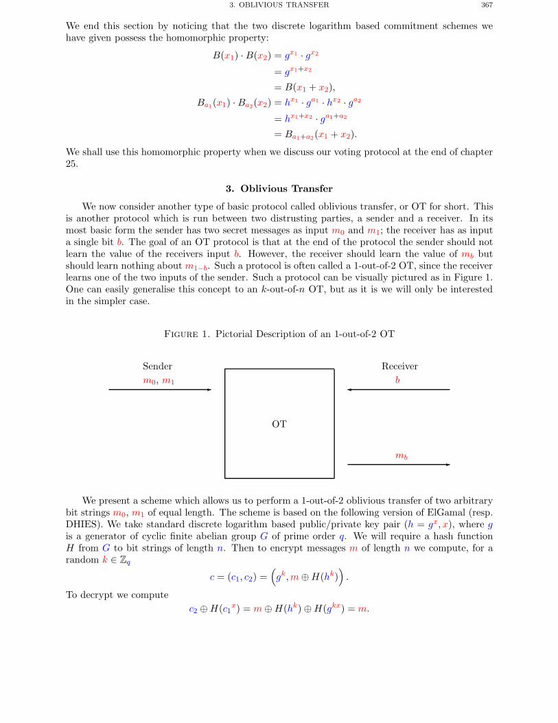
3. OBLIVIOUS TRANSFER 367
We end this section by noticing that the two discrete logarithm based commitment schemes wehave given possess the homomorphic property:
B(x1) · B(x2) = gx1 · gx2
= gx1+x2
= B(x1 + x2),
Ba1(x1) ·Ba2(x2) = hx1 · ga1 · hx2 · ga2= hx1+x2 · ga1+a2
= Ba1+a2(x1 + x2).
We shall use this homomorphic property when we discuss our voting protocol at the end of chapter25.
3. Oblivious Transfer
We now consider another type of basic protocol called oblivious transfer, or OT for short. Thisis another protocol which is run between two distrusting parties, a sender and a receiver. In itsmost basic form the sender has two secret messages as input m0 and m1; the receiver has as inputa single bit b. The goal of an OT protocol is that at the end of the protocol the sender should notlearn the value of the receivers input b. However, the receiver should learn the value of mb butshould learn nothing about m1−b. Such a protocol is often called a 1-out-of-2 OT, since the receiverlearns one of the two inputs of the sender. Such a protocol can be visually pictured as in Figure 1.One can easily generalise this concept to an k-out-of-n OT, but as it is we will only be interestedin the simpler case.
Figure 1. Pictorial Description of an 1-out-of-2 OT
OT
Senderm0, m1
Receiverb
�
mb
We present a scheme which allows us to perform a 1-out-of-2 oblivious transfer of two arbitrarybit strings m0, m1 of equal length. The scheme is based on the following version of ElGamal (resp.DHIES). We take standard discrete logarithm based public/private key pair (h = gx, x), where gis a generator of cyclic finite abelian group G of prime order q. We will require a hash functionH from G to bit strings of length n. Then to encrypt messages m of length n we compute, for arandom k ∈ Zq
c = (c1, c2) =(gk,m⊕H(hk)
).
To decrypt we computec2 ⊕H(c1x) = m⊕H(hk) ⊕H(gkx) = m.
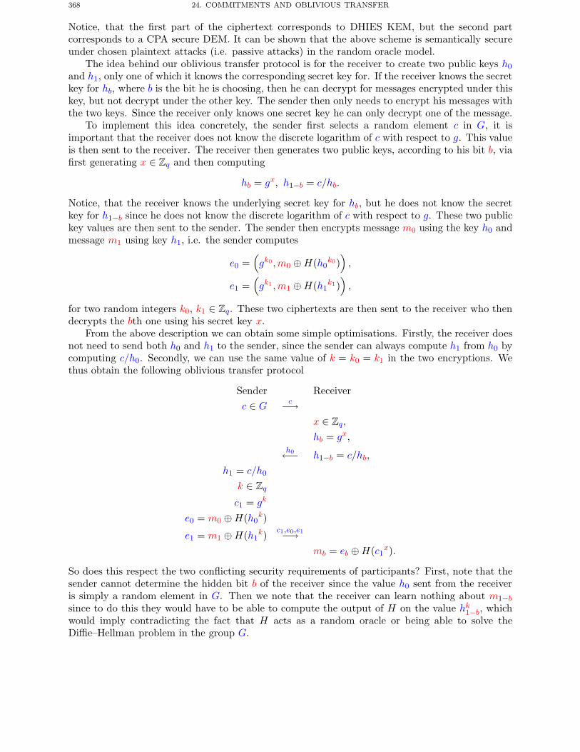
368 24. COMMITMENTS AND OBLIVIOUS TRANSFER
Notice, that the first part of the ciphertext corresponds to DHIES KEM, but the second partcorresponds to a CPA secure DEM. It can be shown that the above scheme is semantically secureunder chosen plaintext attacks (i.e. passive attacks) in the random oracle model.
The idea behind our oblivious transfer protocol is for the receiver to create two public keys h0
and h1, only one of which it knows the corresponding secret key for. If the receiver knows the secretkey for hb, where b is the bit he is choosing, then he can decrypt for messages encrypted under thiskey, but not decrypt under the other key. The sender then only needs to encrypt his messages withthe two keys. Since the receiver only knows one secret key he can only decrypt one of the message.
To implement this idea concretely, the sender first selects a random element c in G, it isimportant that the receiver does not know the discrete logarithm of c with respect to g. This valueis then sent to the receiver. The receiver then generates two public keys, according to his bit b, viafirst generating x ∈ Zq and then computing
hb = gx, h1−b = c/hb.
Notice, that the receiver knows the underlying secret key for hb, but he does not know the secretkey for h1−b since he does not know the discrete logarithm of c with respect to g. These two publickey values are then sent to the sender. The sender then encrypts message m0 using the key h0 andmessage m1 using key h1, i.e. the sender computes
e0 =(gk0,m0 ⊕H(h0
k0)),
e1 =(gk1,m1 ⊕H(h1
k1)),
for two random integers k0, k1 ∈ Zq. These two ciphertexts are then sent to the receiver who thendecrypts the bth one using his secret key x.
From the above description we can obtain some simple optimisations. Firstly, the receiver doesnot need to send both h0 and h1 to the sender, since the sender can always compute h1 from h0 bycomputing c/h0. Secondly, we can use the same value of k = k0 = k1 in the two encryptions. Wethus obtain the following oblivious transfer protocol
Sender Receiverc ∈ G c−→
x ∈ Zq,
hb = gx,h0←− h1−b = c/hb,
h1 = c/h0
k ∈ Zq
c1 = gk
e0 = m0 ⊕H(h0k)
e1 = m1 ⊕H(h1k)
c1,e0,e1−→mb = eb ⊕H(c1x).
So does this respect the two conflicting security requirements of participants? First, note that thesender cannot determine the hidden bit b of the receiver since the value h0 sent from the receiveris simply a random element in G. Then we note that the receiver can learn nothing about m1−bsince to do this they would have to be able to compute the output of H on the value hk1−b, whichwould imply contradicting the fact that H acts as a random oracle or being able to solve theDiffie–Hellman problem in the group G.
Further Reading 369
Chapter Summary
• We introduced the idea of protocols between mutually untrusting parties, and introducedcommitment and oblivious transfer as two simple examples of such protocols.
• A commitment scheme allows one party to bind themselves to a value, and then reveal itlater.
• A commitment scheme needs to be both binding and concealing. Efficient schemes existwhich are either information theoretically binding or information theoretically concealing,but not both.
• An oblivious transfer protocol allows a sender to send one of two messages to a recipient,but he does not know which message is actually obtained. The receiver also learns nothingabout the other message which was sent.
Further Reading
The above oblivious transfer protocol originally appeared, in a slightly modified form in thepaper by Bellare and Micali. The paper by Naor and Pinkas discusses a number of optimisationsof the oblivious transfer protocol which we presented above. In particular it presents mechanismsto perform efficiently 1-out-of-N oblivious transfer.
M. Bellare and S. Micali. Non-interactive oblivious transfer and applications. In Advances inCryptology – Crypto ’89, Springer-Verlag LNCS 435, 547–557, 1990.
M. Naor and B. Pinkas. Efficient oblivious transfer protocols. In SIAM Symposium on DiscreteAlgorithms – SODA 2001.

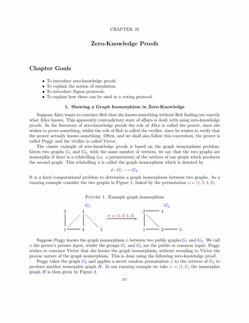
CHAPTER 25
Zero-Knowledge Proofs
Chapter Goals
• To introduce zero-knowledge proofs.• To explain the notion of simulation.• To introduce Sigma protocols.• To explain how these can be used in a voting protocol.
1. Showing a Graph Isomorphism in Zero-Knowledge
Suppose Alice wants to convince Bob that she knows something without Bob finding out exactlywhat Alice knows. This apparently contradictory state of affairs is dealt with using zero-knowledgeproofs. In the literature of zero-knowledge proofs the role of Alice is called the prover, since shewishes to prove something, whilst the role of Bob is called the verifier, since he wishes to verify thatthe prover actually knows something. Often, and we shall also follow this convention, the prover iscalled Peggy and the verifier is called Victor.
The classic example of zero-knowledge proofs is based on the graph isomorphism problem.Given two graphs G1 and G2, with the same number of vertices, we say that the two graphs areisomorphic if there is a relabelling (i.e. a permutation) of the vertices of one graph which producesthe second graph. This relabelling φ is called the graph isomorphism which is denoted by
φ : G1 −→ G2.
It is a hard computational problem to determine a graph isomorphism between two graphs. As arunning example consider the two graphs in Figure 1, linked by the permutation φ = (1, 2, 4, 3).
Figure 1. Example graph isomorphism
G1
1�
��
2
3
4
5
σ = (1, 2, 4, 3)
G2
1
2
3
4
5
Suppose Peggy knows the graph isomorphism φ between two public graphs G1 and G2. We callφ the prover’s private input, whilst the groups G1 and G2 are the public or common input. Peggywishes to convince Victor that she knows the graph isomorphism, without revealing to Victor theprecise nature of the graph isomorphism. This is done using the following zero-knowledge proof.
Peggy takes the graph G2 and applies a secret random permutation ψ to the vertices of G2 toproduce another isomorphic graph H. In our running example we take ψ = (1, 2), the isomorphicgraph H is then given by Figure 2.
371
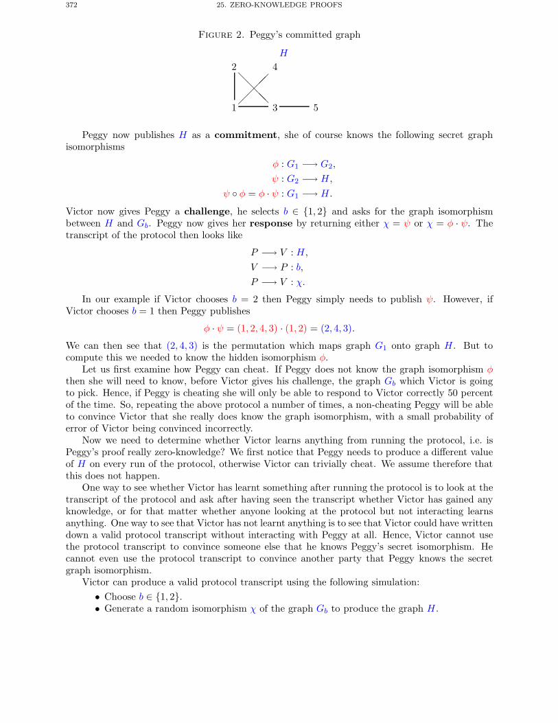
372 25. ZERO-KNOWLEDGE PROOFS
Figure 2. Peggy’s committed graph
H
1�
���
2
3
4
5
Peggy now publishes H as a commitment, she of course knows the following secret graphisomorphisms
φ : G1 −→ G2,
ψ : G2 −→ H,
ψ ◦ φ = φ · ψ : G1 −→ H.
Victor now gives Peggy a challenge, he selects b ∈ {1, 2} and asks for the graph isomorphismbetween H and Gb. Peggy now gives her response by returning either χ = ψ or χ = φ · ψ. Thetranscript of the protocol then looks like
P −→ V : H,V −→ P : b,P −→ V : χ.
In our example if Victor chooses b = 2 then Peggy simply needs to publish ψ. However, ifVictor chooses b = 1 then Peggy publishes
φ · ψ = (1, 2, 4, 3) · (1, 2) = (2, 4, 3).
We can then see that (2, 4, 3) is the permutation which maps graph G1 onto graph H. But tocompute this we needed to know the hidden isomorphism φ.
Let us first examine how Peggy can cheat. If Peggy does not know the graph isomorphism φthen she will need to know, before Victor gives his challenge, the graph Gb which Victor is goingto pick. Hence, if Peggy is cheating she will only be able to respond to Victor correctly 50 percentof the time. So, repeating the above protocol a number of times, a non-cheating Peggy will be ableto convince Victor that she really does know the graph isomorphism, with a small probability oferror of Victor being convinced incorrectly.
Now we need to determine whether Victor learns anything from running the protocol, i.e. isPeggy’s proof really zero-knowledge? We first notice that Peggy needs to produce a different valueof H on every run of the protocol, otherwise Victor can trivially cheat. We assume therefore thatthis does not happen.
One way to see whether Victor has learnt something after running the protocol is to look at thetranscript of the protocol and ask after having seen the transcript whether Victor has gained anyknowledge, or for that matter whether anyone looking at the protocol but not interacting learnsanything. One way to see that Victor has not learnt anything is to see that Victor could have writtendown a valid protocol transcript without interacting with Peggy at all. Hence, Victor cannot usethe protocol transcript to convince someone else that he knows Peggy’s secret isomorphism. Hecannot even use the protocol transcript to convince another party that Peggy knows the secretgraph isomorphism.
Victor can produce a valid protocol transcript using the following simulation:• Choose b ∈ {1, 2}.• Generate a random isomorphism χ of the graph Gb to produce the graph H.
2. ZERO-KNOWLEDGE AND NP 373
• Output the transcript
P −→ V : H,V −→ P : b,P −→ V : χ.
Hence, the interactive nature of the protocol means that it is a zero-knowledge proof. We remarkthat the three-pass system of
commitment −→ challenge −→ response
is the usual characteristic of such protocols.
Just as with commitment schemes we can divide zero-knowledge protocols into categories de-pending on whether they are secure with respect to computationally bounded or unbounded ad-versaries. Clearly two basic properties of an interactive proof system are
• Completeness: If Peggy really knows the thing being proved, then Victor should accepther proof with probability one.
• Soundness: If Peggy does not know the thing being proved, then Victor should only havea small probability of actually accepting the proof.
We usually assume that Victor is a polynomially bounded party, whilst Peggy is unbounded. Inthe above protocol based on graph isomorphism we saw that the soundness probability was equalto one half. Hence, we needed to repeat the protocol a number of times to reduce this to somethingsmall.
The zero-knowledge property we have already noted is related to the concept of a simulation.Suppose the set of valid transcripts (produced by true protocol runs) is denoted by V and let theset of possible simulations be denoted by S. The security is therefore related to how much like theset V is the set S.
A zero-knowledge proof is said to have perfect zero-knowledge if the two sets V and S cannot bedistinguished from each other by a computationally unbounded adversary. However, if the two setsare only indistinguishable by a computationally bounded adversary we say that the zero-knowledgeproof has computational zero-knowledge.
2. Zero-Knowledge and NP
So the question arises as to what can be shown in zero-knowledge. Above we showed thatthe knowledge of whether two graphs are isomorphic can be shown in zero-knowledge. Thus thedecision problem of Graph Isomorphism lies in the set of all decision problems which can be provenin zero-knowledge. But Graph Ismorphism is believed to lie between the complexity classes P andNP -complete, i.e. it can neither be solved in polynomial time, yet neither is it NP -complete.
We can think of NP problems as those problems for which there is a witness (or proof) whichcan be produced by an all powerful prover, but which a polynomially bounded verifier can verifythe proof. However, for the class of NP problems the prover and the verifier do not interact, i.e.the proof is produced and then the verifier verifies it.
If we allow interation then something quite amazing happens. Consider an all powerful proverwho interacts with a polynomially bounded verifier. We wish the prover to convince the verifier ofthe validity of some statement. This is exactly as we had in the previous section except that weonly require the completeness and soundness properties, i.e. we do not require the zero-knowledgeproperty. The decision problems which can be proved to be true in such a manner form thecomplexity class of interactive proofs, or IP . It can be shown that the complexity class IP is equalto the complexity class PSPACE, i.e. the set of all decision problems which can be solved using
374 25. ZERO-KNOWLEDGE PROOFS
polynomial space. It is widely believed that NP�PSPACE, which implies that having interactionreally gives us something extra.
So what happens to interactive proofs when we add in the zero-knowledge requirement? Wecan define a complexity class CZK of all decision problems which can be verified to be true us-ing a computational zero-knowledge proof. We have already shown that the problem of GraphIsomorhism lies in CZK, but this might not include all of the NP problems.
However, since 3-colourability is NP -complete, we have the following elegant proof that NP ⊂CZK,
Theorem 25.1. The problem of 3-colourability of a graph lies in CZK, assuming a computa-tionally hiding commitment scheme exists.
Proof. Consider a graph G = (V ,E) in which the prover knows a colouring ψ of the G,i.e. a map ψ : V → {1, 2, 3} such that ψ(v1) �= ψ(v2) if (v1, v2) ∈ E. The prover first selects acommitment scheme C(x; r) and a random permutation π of the set {1, 2, 3}. Note, the functionπ(ψ(v)) defines another three colouring of the graph. Now the prover commits to this second threecolouring by sending to the verifier the commitments
ci = C (π(ψ(vi)); ri) for all vi ∈ V .
The verifier then selects a random edge (vi, vj) ∈ E and sends this to the prover. The prover nowdecommits to the values of
π(ψ(vi)) and π(ψ(vj)),and the verifier checks that
π(ψ(vi)) �= π(ψ(vj)).We now turn to the three required properties of a zero-knowledge proof.
Completeness: The above protocol is complete since any valid prover will get the verifier toaccept with probability one.Soundness: If we have a cheating prover then at least one edge is invalid, and with probabilityat least 1/|E| the verifier will select an invalid edge. Thus with probability at most 1 − 1/|E| acheating prover will get a verifier to accept. By repeating the above proof many times one canreduce this probability to as low a value as we require.Zero-Knowledge: Assuming the commitment scheme is computationally hiding the obvious sim-ulation and the real protocol will be computationally indistinguishable. �
Notice, that this is a very powerful result. It says that virtually any statement which is liketo come up in cryptography can be proved in zero-knowledge. Clearly the above proof would notprovide a practical implementation, but at least we know that very powerful tools can be applied.In the next section we turn to more practical proofs which can be applied in practice. But beforedoing that we note that the above result can be extended even further
Theorem 25.2. Assuming one-way functions exist then CZK = IP , and hence CZK =PSPACE.
3. Sigma Protocols
One can use a zero-knowledge proof of possession of some secret as an identification scheme.The trouble with the above protocol for graph isomorphisms is that it is not very practical. Thedata structures required are very large, and the protocol needs to be repeated a large number oftimes before Victor is convinced that Peggy really knows the secret.
However one can do even better in many instances if one restricts to so called honest-verifierzero-knowledge protocols. In the case of honest-verifier’s one assumes that the verifier respondsrandomly to the commitment. In other words the verifier’s challenge is uniformly distributed over
3. SIGMA PROTOCOLS 375
the range of possible challenges and does not depend on the value of the prior commitment. Athree round honest-verifier zero-knowledge protocol is often called a Sigma protocol.
For Sigma protocols we can use a different form of soundness called special-soundness, whichis often easier to use in practice. A three round protocol as above is said to have the special-soundness property if given two protocol runs with the same commitment but different challengesone can recover the provers secret. We note that in the case of honest-verifiers the special-soundnessproperty imples the usual soundness property.
The previous zero knowledge protocol based on graph isomorphism was very inefficient, in thatit needed to be repeated a large number of times to reduce the soundness probability to somethingsuitably small. However, if we restrict to Sigma protocols we can be more efficient.
3.1. Schnorr’s Identification Protocol. In essence we have already seen a Sigma protocolwhich has better bandwidth and error properties when we discussed Schnorr signatures in Chap-ter 14. Suppose Peggy’s secret is now the discrete logarithm x of y with respect to g in some finiteabelian group G of prime order q.
The protocol for proof of knowledge now goes as follows
P −→ V : r = gk for a random k,
V −→ P : e,
P −→ V : s = k + xe (mod q).
Victor now verifies that Peggy knows the secret discrete logarithm x by verifying that
r = gsy−e.
Let us examine this protocol in more detail. We first note that the protocol is complete, in thatif Peggy actually knows the discrete logarithm then Victor will accept the protocol.
We now turn to soundness, if Peggy does not know the discrete logarithm x then one caninformly argue that she will only be able to cheat with probability 1/q, which is much better thanthe 1/2 from the earlier graph isomorphism based protocol. We can however show that the protocolhas the special-soundness property; Suppose that we have two protocol runs with transcripts
(r, e, s) and (r, e′, s′).
Note, that the commitments are equal but that the challenges (and hence responses) are different.We need to show that we can from this data recover x. As the protocol verifies this implies thatwe must have
r = gsy−e = gs′y−e
′= r.
Which impliess+ x(−e) = s′ + x(−e′) (mod q).
Hence, we recover x via
x =s− s′
e− e′(mod q).
Notice, that this proof of soundness is almost exactly the same as our argument via the forkinglemma that Schnorr signatures are secure with respect to passive adversaries in the random oraclemodel, Theorem 20.1.
But does Victor learn anything from the protocol? The answer to this is no, since Victor couldsimulate the whole transcript in the following way.
• Generate a random value of e modulo q.• Compute r = gsy−e.
376 25. ZERO-KNOWLEDGE PROOFS
• Output the transcript
P −→ V : r,V −→ P : e,P −→ V : s.
In other words the protocol is zero-knowledge, in that someone cannot tell the simulation of atranscript from a real transcript. This is exactly the same simulation we used when showing thatSchnorr signature are secure against active adversaries in Section 2.2.1.
One problem with the above Sigma protocols is that they are interactive in nature:
P −→ V : Co,V −→ P : Ch,P −→ V : Re,
where Co is the commitment, Ch is the challenge and Re is the response. They can easily be madenon-interactive by replacing the challenge with the evaluation of a cryptographic hash functionapplied to the commitment,
Ch = H(Co).The idea here is that the prover cannot fix the challenge before coming up with the commit-ment, since that would imply they could invert the hash function. The non-interactive protocol nolonger has the zero-knowledge property, since it is not simulatable. In addition a computationallyunbounded Peggy could invert the hash function, hence we need to restrict the prover to be com-putationally bounded. In such a situation, where we restrict to a computationally bounded prover,we say we have a zero-knowledge argument as opposed to a zero-knowledge proof.
One could also add some other data into the value which is hashed, for example a message. Inthis way we turn an interactive Sigma protocol into a digital signature scheme,
Ch = H(Co‖Message).
You should now be able to see how Schnorr signatures are exactly what one obtains when one usesthe hash of the commitment and a message as the challenge, in the above proof of knowledge ofdiscrete logarithms. This transformation, of Sigma protocols into signature schemes, is called theFiat–Shamir heuristic.
Before we discuss other Sigma protocols we introduce some notation, to aid our discussion.Suppose we wish to prove knowledge of the variable x via a Sigma protocol, we then let
• R(x, k) denote the algorithm used to compute the commitmemt r, where k is a randomnonce.
• c is the challenge.• S(c, x, k) denote the algorithm which the prover uses to compute their response s response.• V (r, c, s) will denote the verification algorithm.• S′(c, s) denotes the simulators algorithm which creates a value of a commitment r which
will verify the transcript (r, c, s).All algorithms are assumed to implicitly have as input the public value which x is linked to.
Using this notation Schnorr’s identification protocol becomes the following; The variable wewish to prove knowledge of is x where y = gx. We then have
R(x, k) = r = gk,
S(c, x, k) = s = k + c · x (mod q),V (r, c, s) = true ⇔ (gs = r · y−c),S′(c, s) = r = gs · yc.
3. SIGMA PROTOCOLS 377
3.2. Chaum–Pedersen Protocol. We now present a Sigma protocol called the Chaum–Pedersen protocol which was first presented in the context of electronic cash systems, but whichhas very wide application.
Suppose Peggy wishes to prove she knows two discrete logarithms
y1 = gx1 and y2 = hx2
such that x1 = x2, i.e. we wish to present both a proof of knowledge of the discrete logarithm,but also a proof of equality of the hidden discrete logarithms. We assume that g and h generategroups of prime order q, and we denote the common discrete logarithm by x ease notation. Usingour prior notation for Sigma protocols, the Chaum–Pedersen protocol can be expressed via
R(x, k) = (r1, r2) = (gk, hk),S(c, x, k) = s = k − c · x (mod q),
V ((r1, r2), c, s) = true ⇔ (r1 = gs · yc1 and r2 = hs · yc2) ,S′(c, s) = (r1, r2) = (gs · yc1, hs · yc2).
Note, how this resembles two concurrent runs of the Schnorr protocol.The Chaum–Pedersen protocol is clearly both complete and has the zero-knowledge property,
the second fact follows since the simulation S′(c, s) produces transcripts which are is indistin-guishable from a real transcript. We need to show it is sound, however since we are assuminghonest-verifiers we only need to show it has the special-soundness property. Hence, we assume twoprotocol runs with the same commitments (t1, t2), different challenges, c1 and c2 and valid responsess1 and s2. With this data we need to show that this reveals the common discrete logarithm. Sincethe two transcripts pass the verification test we have such that
t1 = gs1 · yc11 = gs2 · yc21 and t2 = hs1 · yc12 = hs2 · yc22But this implies that
yc1−c21 = gs2−s1 and yc2−c12 = hs2−s1
Hence, the two discrete logarithms are equal and can be extracted from
x =c1 − c2s2 − s1
(mod q).
3.3. Proving Knowledge of Pedersen Commitments. Often one commits to a value usinga commitment scheme, but the receiver is not willing to proceed unless one proves one knows thevalue committed to. In other words the reciever will only proceed if he knows that the sender willat some point be able to reveal the value committed to.
For the commitment schemeB(x) = gx
this is simple, we simply execute Schnorr’s protocol for proof of knowledge of a discrete logarithm.For Pedersen commitments
Ba(x) = hxga
we need something different.In essence we wish to prove knowledge of x1 and x2 such that
y = g1x1 · g2x2
where g1 and g2 are elements in a group of prime order q. We note that the following protocolgeneralises easily to the case when we have more bases, i.e.
y = g1x1 · · · gnxn .
378 25. ZERO-KNOWLEDGE PROOFS
A generalisation which we leave as an exercise.
R(x, k) = (k1, k2) = (r1, r2) = (g1k1 , g2k2),S(c, {x1, x2}, {k1, k2}) = (s1, s2)
= (k1 + c · x1 (mod q), k2 + c · x2 (mod q)) ,V ((r1, r2), c, (s1, s2)) = true ⇔ (gs11 · gs22 = yc · t1 · t2) ,
S′(c, (s1, s2)) = (r1, r2)
=(r1 chosen at random from the group,gs11 · gs22 · yc/r1
).
We leave it to the reader to verify that this protocol is complete, zero-knowledge and satisfies thespecial-soundness property.
3.4. “Or” Proofs. Sometimes the statement about which we wish to execute a Sigma protocolis not as clear cut as the previous examples. For example suppose we wish to show we know eithera secret x or a secret y, without revealing which of the two secrets we know. This is a very commonoccurance which arises in a number of advanced protocols, including the voting protocol we considerlater in this chapter. It turns out that to show knowledge of one thing or another can be performedusing an elegant protocol due to Cramer, Damgard and Schoenmakers.
First assume that there already exists a Sigma protocol to prove knowledge of both secretsindividually. The idea is to combine these two Sigma protocols together into one protocol whichproves the statement we require. The key idea is as follows: For the secret we know we run theSigma protocol as normal, however for the secret we do not know we run the simulated Sigmaprotocol. These two protocols are then linked together by linking the commitments.
As a high level example, suppose the protocol for proving knowledge of x is given by the set ofalgorithms
R1(x, k1), S1(c1, x, k1), V (r1, c1, s1), S′1(c1, s1).
Similarly we let the Sigma protocol to prove knowlegde of y be given by
R2(y, k2), S2(c2, y, k2), V (r2, c2, s2), S′2(c2, s2).
We assume that the challenges c1 and c2 are bit strings of the same length in what follows.Now suppose we know x, but not y, then our algorithms for the combined proof become:
R(x, k1) = (r1, r2)
=
⎧⎨⎩
r1 = R1(x, k1)Select c2, s2 from the correct distributionsr2 = S′
2(c2, s2)S(c, x, k1) = (c1, c2, s1, s2)
={c1 = c⊕ c2s1 = S1(c1, x, k1)
).
V ((r1, r2), c, (c1, c2, s1, s2) = true ⇔c = c1 ⊕ c2 and V1(r1, c1, s1) and V2(r2, c2, s2)
S′(c, (c1, c2, s1, s2)) = (r1, r2)=(S′
1(c1, s1), S′2(c2, s2)
)Note that the prover does not reveal the value of c1, c2 or s2 until the response stage of theprotocol. Also note that in the simulated protocol the correct distributions of c, c1 and c2 are suchthat c = c1⊕c2. The protocol for the case where we know y but not x follows by reversing the rolesof c1 and c2 and r1 and r2 in the algorithms R, S and V . If the prover knows both x and y then
3. SIGMA PROTOCOLS 379
they can execute either of the two possibilties. The completeness, soundness and zero-knowledgeproperties follow from the corresponding properties of the original Sigma protocols.
We now present a simple example which uses the Schnorr protocol as a building block. Supposewe wish to prove knowledge of either x1 or x2 such that
y1 = gx1 and y2 = gx2,
where g lies in a group G of prime order q. We assume that the prover knows xi but not xj wherei �= j.
The provers commitment is (r1, r2) is computed by selecting cj and ki uniformly at randomfrom Fq
∗ and sj uniformly at random from G. They then compute
ri = gki and rj = gsj · y−cjj .
On recieving the challeneg c ∈ Fq∗ the prover computes
ci = c+ cj (mod q)si = ki + ci · xi (mod q).
Note, we have replaced ⊕ in computing the “challenge” ci into addition modulo q, a momentsthought reveals that this is a better way at preserving the relative distributions in this example.The prover then outputs (c1, c2, s1, s2)
The verifier checks the proof by checking that
c = c1 + c2 (mod q) and r1 = gs1 · y−c11 and r2 = gs2 · y−c22 .
These “Or” proofs can be extended to an arbitrary number of disjunctions of statements in theobvious manner: Given n statements of which the prover only knows one secret,
• Simulate n− 1 statements using the simulations and challenges ci• Commit as usual to the known statement• Generate correct challenge for the known statement via
c = c1 ⊕ · · · ⊕ cn
3.5. A more complicated example. We end this section by giving a protocol, which is azero-knowledge argument, which will be required when we discuss voting schemes. It is obtainedby combining the protocol for proving knowledge of Pedersen commitments with the “or” proofsof the prior section.
Consider the earlier commitment scheme given by
Ba(x) = hxga,
where G = 〈g〉 is a finite abelian group of prime order q, h is an element of G whose discretelogarithm with respect to g is unknown, x is the value being committed and a is a random nonce.We are interested in the case where the value committed is restricted to be either plus or minusone, i.e. x ∈ {−1, 1}. It will be important in our application for the person committing to provethat their commitment is from the set {−1, 1} without revealing what the actual value of thecommitment is.
To do this we execute the following protocol.
380 25. ZERO-KNOWLEDGE PROOFS
• As well as publishing the commitment Ba(x), Peggy also chooses random numbers d, rand w modulo q and then publishes α1 and α2 where
α1 =
{gr (Ba(x)h)−d if x = 1gw if x = −1,
α2 =
{gw if x = 1gr(Ba(x)h−1
)−d if x = −1.
• Victor now sends a random challenge c to Peggy.• Peggy responds by setting
d′ = c− d,
r′ = w + ad′.
Then Peggy returns the values
(d1, d2, r1, r2) =
{(d, d′, r, r′) if x = 1(d′, d, r′, r) if x = −1.
• Victor then verifies that the following three equations hold
c = d1 + d2,
gr1 = α1(Ba(x)h)d1 ,
gr2 = α2(Ba(x)h−1)d2 .
To show that the above protocol works we need to show that(1) If Peggy responds honestly then Victor will verify that the above three equations hold.(2) If Peggy has not committed to plus or minus one then she will find it hard to produce a
response to Victor’s challenge which is correct.(3) The protocol reveals no information to any party as to the exact value of Peggy’s commit-
ment, bar that it come from the set {−1, 1}.We leave the verification of these three points to the reader. Note that the above protocol canclearly be conducted in a non-interactive manner by defining
c = H (α1‖α2‖Ba(x)) .4. An Electronic Voting System
In this section we describe an electronic voting system which utilizes some of the primitives wehave been discussing in this chapter and in earlier chapters. In particular we make use of secretsharing schemes from Chapter 23, commitment schemes from Chapter 24, and zero-knowledgeproofs from this chapter. The purpose is to show how basic cryptographic primitives can becombined into a complicated application giving real value. One can consider an electronic votingscheme to be a special form of a secure multi-party computation, a topic which we shall return toin Chapter 26.
Our voting system will assume that we have m voters, and that there are n centres whichperform the tallying. The use of a multitude of tallying centres is to allow voter anonymity andstop a few centres colluding to fix the vote. We shall assume that voters are only given a choice ofone of two candidates, for example Democrat or Republican.
The voting system we shall describe will have the following seven properties.(1) Only authorized voters will be able to vote.(2) No one will be able to vote more than once.(3) No stakeholder will be able to determine how someone else has voted.
4. AN ELECTRONIC VOTING SYSTEM 381
(4) No one can duplicate someone else’s vote.(5) The final result will be correctly computed.(6) All stakeholders will be able to verify that the result was computed correctly.(7) The protocol will work even in the presence of some bad parties.
4.1. System Setup. Each of the n tally centres has a public key encryption function Ei. Weassume a finite abelian group G is fixed, of prime order q, and two elements g, h ∈ G are selectedfor which no party (including the tally centres) know the discrete logarithm
h = gx.
Each voter has a public key signature algorithm.
4.2. Vote Casting. Each of the m voters picks a vote vj from the set {−1, 1}. The voterpicks a random blinding value aj ∈ Z/qZ and publishes their vote
Bj = Baj (vj),
using the bit commitment scheme given earlier. This vote is public to all participating parties, bothtally centres and other voters. Along with the vote Bj the voter also publishes a non-interactiveversion of the earlier protocol to show that the vote was chosen from the set {−1, 1}. The vote andits proof are then digitally signed using the signing algorithm of the voter.
4.3. Vote Distribution. We now need to distribute the votes cast around the tally centresso that the final tally can be computed. Each voter employs Shamir secret sharing as follows, toshare the aj and vj around the tallying centres: Each voter picks two random polynomials moduloq of degree t < n.
Rj(X) = vj + r1,jX + · · · + rt,jXt,
Sj(X) = aj + s1,jX + · · · + st,jXt.
The voter computes(ui,j , wi,j) = (Rj(i), Sj(i)) for 1 ≤ i ≤ n.
The voter encrypts the pair (ui,j, wi,j) using the ith tally centre’s encryption algorithm Ei. Thisencrypted share is sent to the relevant tally centre. The voter then publishes it commitments tothe polynomial Rj(X) by publicly posting
Bl,j = Bsl,j (rl,j) for 1 ≤ l ≤ t,
again using the earlier commitment scheme.
4.4. Consistency Check. Each centre i needs to check that the values of
(ui,j, wi,j)
it has received from voter j are consistent with the commitments made by the voter. This is doneby verifying the following equation
Bj
t∏l=1
Bl,jil = Baj (vj)
t∏l=1
Bsl,j(rl,j)il
= hvjgajt∏l=1
(hrl,jgsl,j)il
= h(vj+Ptl=1 rl,ji
l)g(aj+Ptl=1 sl,j i
l)
= hui,jgwi,j .
382 25. ZERO-KNOWLEDGE PROOFS
4.5. Tally Counting. Each of the n tally centres now computes and publicly posts its sumof the shares of the votes cast
Ti =m∑j=1
ui,j
plus it posts its sum of shares of the blinding factors
Ai =m∑j=1
wi,j.
Every other party, both other centres and voters can check that this has been done correctly byverifying that
m∏j=1
(Bj
t∏l=1
Bl,jjl
)=
m∏j=1
hui,jgwi,j
= hTigAi .
Any party can compute the final tally by taking t of the values Ti and interpolating them to revealthe final tally. This is because Ti is the evaluation at i of a polynomial which shares out the sumof the votes. To see this we have
Ti =m∑j=1
ui,j
=m∑j=1
Rj(i)
=
⎛⎝ m∑j=1
vj
⎞⎠+
⎛⎝ m∑j=1
r1,j
⎞⎠ i+ · · · +
⎛⎝ m∑j=1
rt,j
⎞⎠ it.
If the final tally is negative then the majority of people voted −1, whilst if the final tally is positivethen the majority of people voted +1. You should now convince yourself that the above protocolhas the seven properties we said it would at the beginning.
Chapter Summary
• An interactive proof of knowledge leaks no information if the transcript could be simulatedwithout the need of the secret information.
• Both interactive proofs and zero-knowledge proofs are a very powerful construct, they canbe used to prove any statement in PSPACE.
• Interactive proofs of knowledge can be turned into digital signature algorithms by replacingthe challenge by the hash of the commitment concatenated with the message.
• Quite complicated protocols can then be built on top of our basic primitives of encryption,signatures, commitment and zero-knowledge proofs. As an example we gave an electronicvoting protocol.
Further Reading

Further Reading 383
The book by Goldreich has more details on zero-knowledge proofs, whilst a good overview ofthis area is given in Stinson’s book. The voting scheme we describe is given in the paper of Crameret al. from EuroCrypt.
R. Cramer, M. Franklin, B. Schoenmakers and M. Yung. Multi-authority secret-ballot electionswith linear work. In Advances in Cryptology – EuroCrypt ’96, Springer-Verlag LNCS 1070, 72–83,1996.
O. Goldreich. Modern Cryptography, Probabilistic Proofs and Pseudo-randomness. Springer-Verlag,1999.
D. Stinson. Cryptography: Theory and Practice. CRC Press, 1995.

CHAPTER 26
Secure Multi-Party Computation
Chapter Goals
• To introduce the concept of multi-party computation.• To present a two-party protocol based on Yao’s garbled circuit construction.• To present a multi-party protocol based on Shamir secret sharing.
1. Introduction
Secure multi-party computation is an area of cryptography which deals with two or more playerscomputing a function on their private inputs. They wish to do so in a way which means that theirprivate inputs still remain private. Of course depending on the function being computed, someinformation about the inputs may leak. The classical example is the so-called millionaires problem;suppose a bunch of millionaires have a lunch time meeting at an expensive restaurant and decidethat the richest of them will pay the bill. However, they do not want to reveal their actual wealthto each other. This is an example of a secure multi-party computation. The inputs are the valuesxi, which denote the wealth of each party, and the function to be computed is
f(x1, . . . , xn) = i where xi > xj for all i �= j.
Clearly if we compute such a function then some information about party i’s value leaks, i.e. thatit is greater than all the other values. However, we require in secure multi-party computation thatthis is the only information which leaks.
One can consider a number of our previous protocols as being examples of secure multi-partycomputation. For example, the voting protocol given previously involves the computation of theresult of each party voting, without anyone learning the vote being cast by a particular party.
One solution to securely evaluating a function is for all the parties to send their inputs to atrusted third party. This trusted party then computes the function and passes the output back tothe parties. However, we want to remove such a trusted third party entirely. Intuitively a multi-party computation is said to be secure if the information which is leaked is precisely that whichwould have leaked if the computation had been conducted by encrypting messages to a trustedthird party.
This is not the only security issue which needs to be addressed when considering secure multi-party computation. There are two basic security models: In the first model the parties are guaran-teed to follow the protocols, but are interested in breaking the privacy of their fellow participants.Such adversaries are called honest-but-curious, and they in some sense correspond to passive ad-versaries in other areas of cryptography. Whilst honest-but-curious adversaries follow the protocol,a number of them could combine their different internal data so as to subvert the security of thenon-corrupt parties. In the second model the adversaries can deviate from the protocol and maywish to pass incorrect data around so as to subvert the computation of the function. Again weallow such adversaries to talk to each other in a coalition. Such adversaries are called malicious.
385
386 26. SECURE MULTI-PARTY COMPUTATION
There is a problem though, if we assume that communication is asynchronous, which is themost practically relevant situation, then some party must go last. In such a situation one partymay have learnt the outcome of the computation, but one party may not have the value yet (namelythe party which receives the last message). Any malicious party can clearly subvert the protocolby not sending the last message. Usually malicious adversaries are assumed not to perform suchan attack. A protocol which is said to be secure against an adversary which can delete the finalmessage is said to be fair.
In what follows we shall mainly explain the basic ideas behind secure multi-party computationin the case of honest-but-curious adversaries. We shall touch on the case of malicious adversariesfor one of our examples though, as it provides a nice example of an application of various propertiesof Shamir secret sharing.
If we let n denote the number of parties which engage in the protocol, we would like to createprotocols for secure multi-party computation which are able to tolerate a large number of corruptparties. It turns out that there is a theoretical limit as to the number of parties which can betolerated as being corrupt. For the case of honest-but-curious adversaries we can tolerate up ton/2 corrupt parties. However, for malicious adversaries we can tolerate up to n/2 corrupt partiesonly if we base our security on some computational assumption, for example the inability to breaka symmetric encryption scheme. If we are interested in perfect security then we can only tolerateup to n/3 corrupt parties in the malicious case.
Protocols for secure multi-party computation usually fall into one of two distinct families. Thefirst is based on an idea of Yao called a garbled circuit or Yao circuit, in this case one presents thefunction to be computed as a binary circuit, and then one “encrypts” the gates of this circuit toform the garbled circuit. This approach is clearly based on a computational assumption, i.e. thatthe encryption scheme is secure. The second approach is based on secret sharing schemes; here oneusually represents the function to be computed as an arithmetic circuit. In this second approachone uses a perfect secret sharing scheme to obtain perfect security.
It turns out that the first approach seems better suited to the case where there are two parties,whilst the second approach is better suited to the case of three of more parties. In our discussionbelow we will present a computationally secure solution for the two party case in the presence ofhonest-but-curious adversaries, based on Yao circuits. This approach can be extended to morethan two parties, and to malicious adversaries, but doing this is beyond the scope of this book. Wethen present a protocol for the multi-party case which is perfectly secure. We sketch two versions,one which provides security against honest-but-curious adversaries and one which provides securityagainst malicious adversaries.
2. The Two-Party Case
We shall in this section consider the method of secure multi-party computation based on garbledcircuits. We suppose there are two parties A and B each of whome have input x and y, and thatA wishes to compute fA(x, y) and B wishes to compute fB(x, y). Recall this needs to be donewithout B learning anything about x or fA(x, y), except from what he can deduce from fB(x, y)and y, with a similar privacy statement applying to A’s input and outputs.
First note that it is enough for B to receive the output of a related function f . To see this welet A have an extra secret input k which is as long as the maximum output of her function fA(x, y).If we can create a protocol in which B learns the value of the function
f(x, y, k) = (k ⊕ fA(x, y), fB(x, y)),
then B simply sends the value of k ⊕ fA(x, y) back to A who can then decrypt it using k, andso determine fA(x, y). Hence, we will assume that there is only one function which needs to becomputed and that its output will be determined by B.
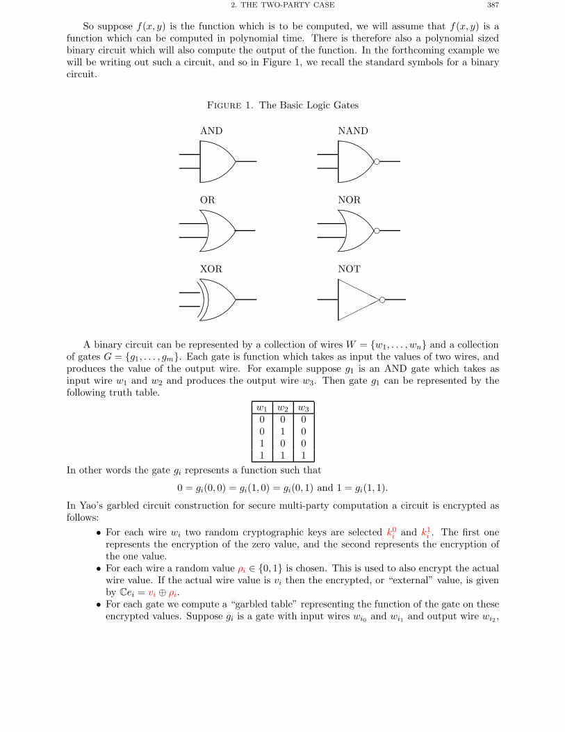
2. THE TWO-PARTY CASE 387
So suppose f(x, y) is the function which is to be computed, we will assume that f(x, y) is afunction which can be computed in polynomial time. There is therefore also a polynomial sizedbinary circuit which will also compute the output of the function. In the forthcoming example wewill be writing out such a circuit, and so in Figure 1, we recall the standard symbols for a binarycircuit.
Figure 1. The Basic Logic Gates
AND
. ................ ................ .................................................................................................
................
. ................ ................ ................. ................. .............................................
...............
...
................
NAND
. ................ ................ .................................................................................................
................
. ................ ................ ................. ................. .............................................
...............
...
................ �
OR
. ................ ................ .................................................................................................
................
. ................ ................ ................. ................. .............................................
...............
...
................
.............
.......
....................
....................
..........
.........
..........
.........
....................
....................
...................
NOR
. ................ ................ .................................................................................................
................
. ................ ................ ................. ................. .............................................
...............
...
................
.............
.......
....................
....................
..........
.........
..........
.........
....................
....................
...................
�
XOR
. ................ ................ .................................................................................................
................
. ................ ................ ................. ................. ..............................................
..............
...
................
..............
......
....................
....................
..........
.........
..........
.........
....................
....................
...................
.................
................
.................
..........
......
..........
......
.................
.................
................
NOT
�����
����� �
A binary circuit can be represented by a collection of wires W = {w1, . . . , wn} and a collectionof gates G = {g1, . . . , gm}. Each gate is function which takes as input the values of two wires, andproduces the value of the output wire. For example suppose g1 is an AND gate which takes asinput wire w1 and w2 and produces the output wire w3. Then gate g1 can be represented by thefollowing truth table.
w1 w2 w3
0 0 00 1 01 0 01 1 1
In other words the gate gi represents a function such that
0 = gi(0, 0) = gi(1, 0) = gi(0, 1) and 1 = gi(1, 1).
In Yao’s garbled circuit construction for secure multi-party computation a circuit is encrypted asfollows:
• For each wire wi two random cryptographic keys are selected k0i and k1
i . The first onerepresents the encryption of the zero value, and the second represents the encryption ofthe one value.
• For each wire a random value ρi ∈ {0, 1} is chosen. This is used to also encrypt the actualwire value. If the actual wire value is vi then the encrypted, or “external” value, is givenby Cei = vi ⊕ ρi.
• For each gate we compute a “garbled table” representing the function of the gate on theseencrypted values. Suppose gi is a gate with input wires wi0 and wi1 and output wire wi2 ,
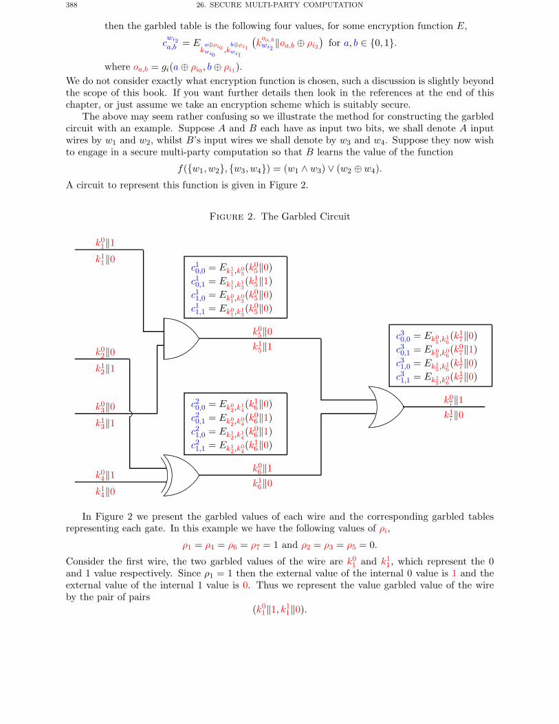
388 26. SECURE MULTI-PARTY COMPUTATION
then the garbled table is the following four values, for some encryption function E,
cwi2a,b = E
ka⊕ρi0wi0
,kb⊕ρi1wi1
(koa,bwi2
‖oa,b ⊕ ρi2)
for a, b ∈ {0, 1}.
where oa,b = gi(a⊕ ρi0 , b⊕ ρi1).We do not consider exactly what encryption function is chosen, such a discussion is slightly beyondthe scope of this book. If you want further details then look in the references at the end of thischapter, or just assume we take an encryption scheme which is suitably secure.
The above may seem rather confusing so we illustrate the method for constructing the garbledcircuit with an example. Suppose A and B each have as input two bits, we shall denote A inputwires by w1 and w2, whilst B’s input wires we shall denote by w3 and w4. Suppose they now wishto engage in a secure multi-party computation so that B learns the value of the function
f({w1, w2}, {w3, w4}) = (w1 ∧ w3) ∨ (w2 ⊕w4).
A circuit to represent this function is given in Figure 2.
Figure 2. The Garbled Circuit
k01‖1k11‖0
.................................
k02‖0k12‖1
k03‖0k13‖1
k04‖1k14‖0
. ................ ................ .................................................................................................
................
. ................ ................ ................. ................. .............................................
...............
...
................
c10,0 = Ek11 ,k
03(k0
5‖0)c10,1 = Ek1
1 ,k13(k1
5‖1)c11,0 = Ek0
1 ,k03(k0
5‖0)c11,1 = Ek0
1 ,k13(k0
5‖0)
. ................ ................ .................................................................................................
................
. ................ ................ ................. ................. .............................................
...............
...
................
..............
......
....................
....................
..........
.........
..........
.........
....................
....................
...................
.................
................
.................
..........
......
..........
......
.................
.................
................
c20,0 = Ek02 ,k
14(k1
6‖0)c20,1 = Ek0
2 ,k04(k0
6‖1)c21,0 = Ek1
2 ,k14(k0
6‖1)c21,1 = Ek1
2 ,k04(k1
6‖0)
k05‖0k15‖1
k06‖1k16‖0
. ................ ................ .................................................................................................
................
. ................ ................ ................. ................. ..............................................
..............
...
................
..............
......
....................
....................
..........
.........
..........
.........
....................
....................
...................
c30,0 = Ek05 ,k
16(k1
7‖0)c30,1 = Ek0
5 ,k06(k0
7‖1)c31,0 = Ek1
5 ,k16(k1
7‖0)c31,1 = Ek1
5 ,k06(k1
7‖0)
k07‖1k17‖0
In Figure 2 we present the garbled values of each wire and the corresponding garbled tablesrepresenting each gate. In this example we have the following values of ρi,
ρ1 = ρ4 = ρ6 = ρ7 = 1 and ρ2 = ρ3 = ρ5 = 0.
Consider the first wire, the two garbled values of the wire are k01 and k1
1 , which represent the 0and 1 value respectively. Since ρ1 = 1 then the external value of the internal 0 value is 1 and theexternal value of the internal 1 value is 0. Thus we represent the value garbled value of the wireby the pair of pairs
(k01‖1, k1
1‖0).
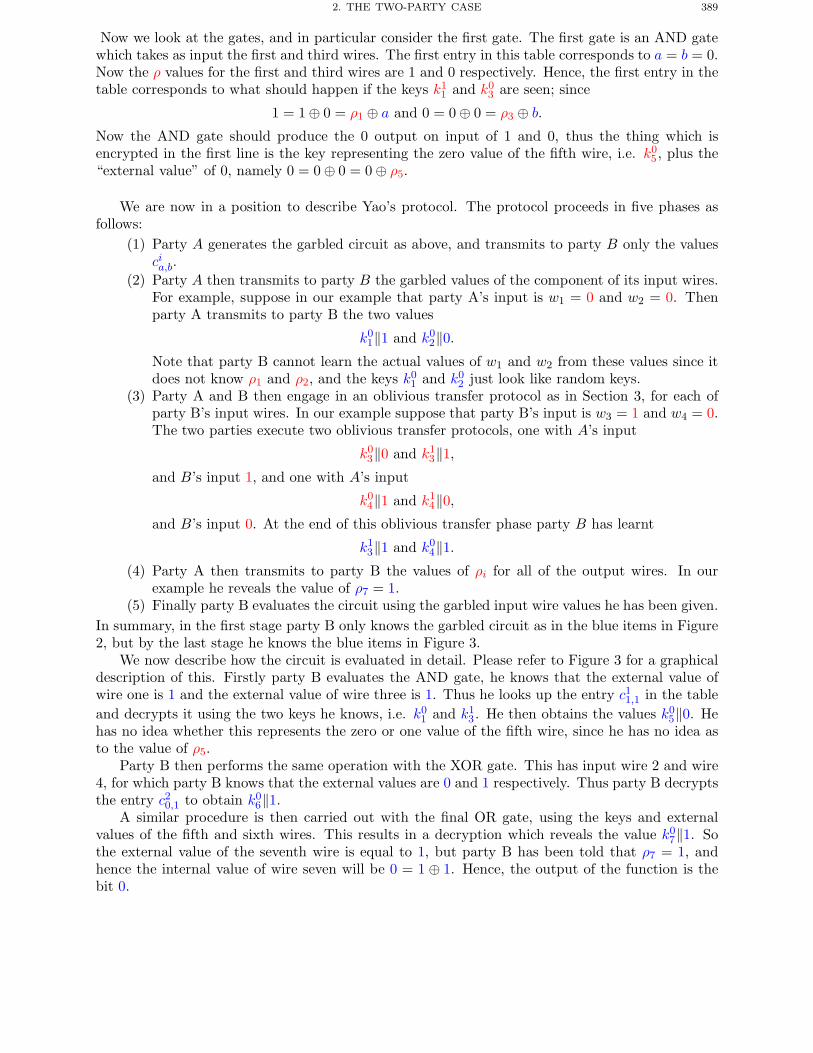
2. THE TWO-PARTY CASE 389
Now we look at the gates, and in particular consider the first gate. The first gate is an AND gatewhich takes as input the first and third wires. The first entry in this table corresponds to a = b = 0.Now the ρ values for the first and third wires are 1 and 0 respectively. Hence, the first entry in thetable corresponds to what should happen if the keys k1
1 and k03 are seen; since
1 = 1 ⊕ 0 = ρ1 ⊕ a and 0 = 0 ⊕ 0 = ρ3 ⊕ b.
Now the AND gate should produce the 0 output on input of 1 and 0, thus the thing which isencrypted in the first line is the key representing the zero value of the fifth wire, i.e. k0
5 , plus the“external value” of 0, namely 0 = 0 ⊕ 0 = 0 ⊕ ρ5.
We are now in a position to describe Yao’s protocol. The protocol proceeds in five phases asfollows:
(1) Party A generates the garbled circuit as above, and transmits to party B only the valuescia,b.
(2) Party A then transmits to party B the garbled values of the component of its input wires.For example, suppose in our example that party A’s input is w1 = 0 and w2 = 0. Thenparty A transmits to party B the two values
k01‖1 and k0
2‖0.Note that party B cannot learn the actual values of w1 and w2 from these values since itdoes not know ρ1 and ρ2, and the keys k0
1 and k02 just look like random keys.
(3) Party A and B then engage in an oblivious transfer protocol as in Section 3, for each ofparty B’s input wires. In our example suppose that party B’s input is w3 = 1 and w4 = 0.The two parties execute two oblivious transfer protocols, one with A’s input
k03‖0 and k1
3‖1,and B’s input 1, and one with A’s input
k04‖1 and k1
4‖0,and B’s input 0. At the end of this oblivious transfer phase party B has learnt
k13‖1 and k0
4‖1.(4) Party A then transmits to party B the values of ρi for all of the output wires. In our
example he reveals the value of ρ7 = 1.(5) Finally party B evaluates the circuit using the garbled input wire values he has been given.
In summary, in the first stage party B only knows the garbled circuit as in the blue items in Figure2, but by the last stage he knows the blue items in Figure 3.
We now describe how the circuit is evaluated in detail. Please refer to Figure 3 for a graphicaldescription of this. Firstly party B evaluates the AND gate, he knows that the external value ofwire one is 1 and the external value of wire three is 1. Thus he looks up the entry c11,1 in the tableand decrypts it using the two keys he knows, i.e. k0
1 and k13 . He then obtains the values k0
5‖0. Hehas no idea whether this represents the zero or one value of the fifth wire, since he has no idea asto the value of ρ5.
Party B then performs the same operation with the XOR gate. This has input wire 2 and wire4, for which party B knows that the external values are 0 and 1 respectively. Thus party B decryptsthe entry c20,1 to obtain k0
6‖1.A similar procedure is then carried out with the final OR gate, using the keys and external
values of the fifth and sixth wires. This results in a decryption which reveals the value k07‖1. So
the external value of the seventh wire is equal to 1, but party B has been told that ρ7 = 1, andhence the internal value of wire seven will be 0 = 1 ⊕ 1. Hence, the output of the function is thebit 0.
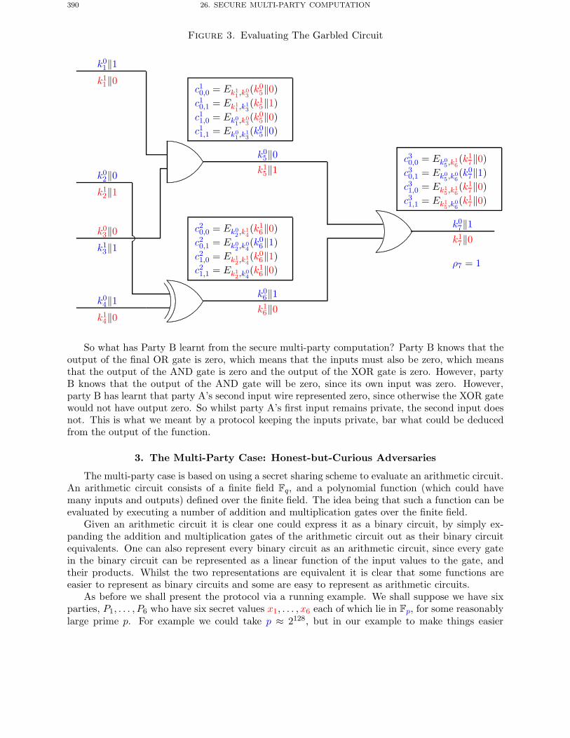
390 26. SECURE MULTI-PARTY COMPUTATION
Figure 3. Evaluating The Garbled Circuit
k01‖1k11‖0
.................................
k02‖0k12‖1
k03‖0k13‖1
k04‖1k14‖0
. ................ ................ .................................................................................................
................
. ................ ................ ................. ................. .............................................
...............
...
................
c10,0 = Ek11 ,k
03(k0
5‖0)c10,1 = Ek1
1 ,k13(k1
5‖1)c11,0 = Ek0
1 ,k03(k0
5‖0)c11,1 = Ek0
1 ,k13(k0
5‖0)
. ................ ................ .................................................................................................
................
. ................ ................ ................. ................. ..............................................
..............
...
................
..............
......
....................
....................
..........
.........
..........
.........
....................
....................
...................
.................
................
.................
..........
......
..........
......
.................
.................
................
c20,0 = Ek02 ,k
14(k1
6‖0)c20,1 = Ek0
2 ,k04(k0
6‖1)c21,0 = Ek1
2 ,k14(k0
6‖1)c21,1 = Ek1
2 ,k04(k1
6‖0)
k05‖0k15‖1
k06‖1k16‖0
. ................ ................ .................................................................................................
................
. ................ ................ ................. ................. .............................................
...............
...
................
.............
.......
....................
....................
..........
.........
..........
.........
....................
....................
...................
c30,0 = Ek05 ,k
16(k1
7‖0)c30,1 = Ek0
5 ,k06(k0
7‖1)c31,0 = Ek1
5 ,k16(k1
7‖0)c31,1 = Ek1
5 ,k06(k1
7‖0)
k07‖1k17‖0
ρ7 = 1
So what has Party B learnt from the secure multi-party computation? Party B knows that theoutput of the final OR gate is zero, which means that the inputs must also be zero, which meansthat the output of the AND gate is zero and the output of the XOR gate is zero. However, partyB knows that the output of the AND gate will be zero, since its own input was zero. However,party B has learnt that party A’s second input wire represented zero, since otherwise the XOR gatewould not have output zero. So whilst party A’s first input remains private, the second input doesnot. This is what we meant by a protocol keeping the inputs private, bar what could be deducedfrom the output of the function.
3. The Multi-Party Case: Honest-but-Curious Adversaries
The multi-party case is based on using a secret sharing scheme to evaluate an arithmetic circuit.An arithmetic circuit consists of a finite field Fq, and a polynomial function (which could havemany inputs and outputs) defined over the finite field. The idea being that such a function can beevaluated by executing a number of addition and multiplication gates over the finite field.
Given an arithmetic circuit it is clear one could express it as a binary circuit, by simply ex-panding the addition and multiplication gates of the arithmetic circuit out as their binary circuitequivalents. One can also represent every binary circuit as an arithmetic circuit, since every gatein the binary circuit can be represented as a linear function of the input values to the gate, andtheir products. Whilst the two representations are equivalent it is clear that some functions areeasier to represent as binary circuits and some are easy to represent as arithmetic circuits.
As before we shall present the protocol via a running example. We shall suppose we have sixparties, P1, . . . , P6 who have six secret values x1, . . . , x6 each of which lie in Fp, for some reasonablylarge prime p. For example we could take p ≈ 2128, but in our example to make things easier
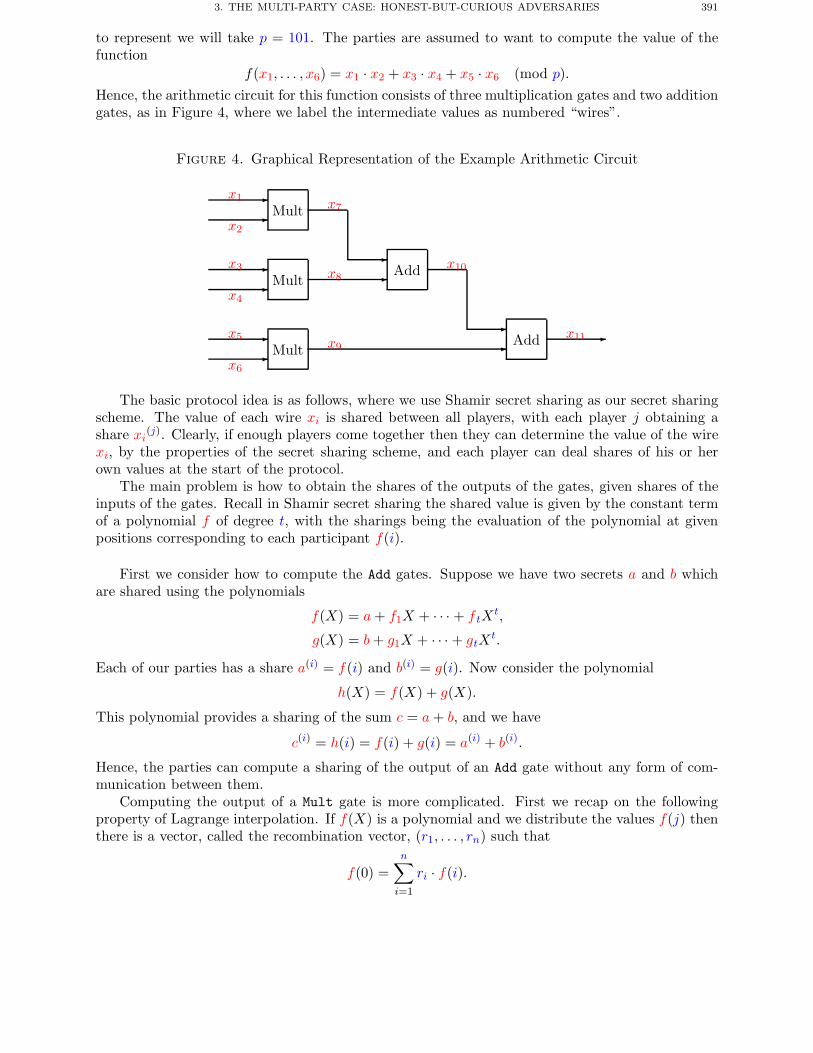
3. THE MULTI-PARTY CASE: HONEST-BUT-CURIOUS ADVERSARIES 391
to represent we will take p = 101. The parties are assumed to want to compute the value of thefunction
f(x1, . . . , x6) = x1 · x2 + x3 · x4 + x5 · x6 (mod p).Hence, the arithmetic circuit for this function consists of three multiplication gates and two additiongates, as in Figure 4, where we label the intermediate values as numbered “wires”.
Figure 4. Graphical Representation of the Example Arithmetic Circuit
x1
x2
Mult
x3
x4
Mult
x5
x6
Mult
x7
x8 Add x10
x9 Add x11
The basic protocol idea is as follows, where we use Shamir secret sharing as our secret sharingscheme. The value of each wire xi is shared between all players, with each player j obtaining ashare xi(j). Clearly, if enough players come together then they can determine the value of the wirexi, by the properties of the secret sharing scheme, and each player can deal shares of his or herown values at the start of the protocol.
The main problem is how to obtain the shares of the outputs of the gates, given shares of theinputs of the gates. Recall in Shamir secret sharing the shared value is given by the constant termof a polynomial f of degree t, with the sharings being the evaluation of the polynomial at givenpositions corresponding to each participant f(i).
First we consider how to compute the Add gates. Suppose we have two secrets a and b whichare shared using the polynomials
f(X) = a+ f1X + · · · + f tXt,
g(X) = b+ g1X + · · · + gtXt.
Each of our parties has a share a(i) = f(i) and b(i) = g(i). Now consider the polynomial
h(X) = f(X) + g(X).
This polynomial provides a sharing of the sum c = a+ b, and we have
c(i) = h(i) = f(i) + g(i) = a(i) + b(i).
Hence, the parties can compute a sharing of the output of an Add gate without any form of com-munication between them.
Computing the output of a Mult gate is more complicated. First we recap on the followingproperty of Lagrange interpolation. If f(X) is a polynomial and we distribute the values f(j) thenthere is a vector, called the recombination vector, (r1, . . . , rn) such that
f(0) =n∑i=1
ri · f(i).
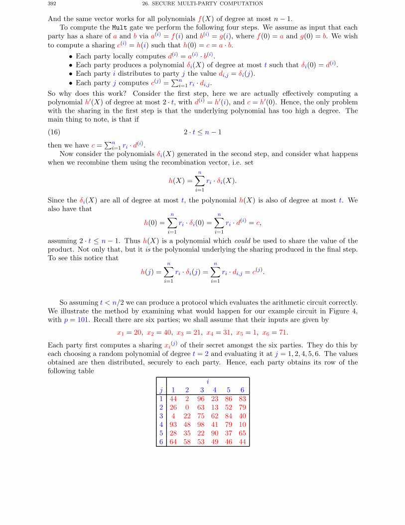
392 26. SECURE MULTI-PARTY COMPUTATION
And the same vector works for all polynomials f(X) of degree at most n− 1.To compute the Mult gate we perform the following four steps. We assume as input that each
party has a share of a and b via a(i) = f(i) and b(i) = g(i), where f(0) = a and g(0) = b. We wishto compute a sharing c(i) = h(i) such that h(0) = c = a · b.
• Each party locally computes d(i) = a(i) · b(i).• Each party produces a polynomial δi(X) of degree at most t such that δi(0) = d(i).• Each party i distributes to party j the value di,j = δi(j).• Each party j computes c(j) =
∑ni=1 ri · di,j.
So why does this work? Consider the first step, here we are actually effectively computing apolynomial h′(X) of degree at most 2 · t, with d(i) = h′(i), and c = h′(0). Hence, the only problemwith the sharing in the first step is that the underlying polynomial has too high a degree. Themain thing to note, is that if
(16) 2 · t ≤ n− 1
then we have c =∑n
i=1 ri · d(i).Now consider the polynomials δi(X) generated in the second step, and consider what happens
when we recombine them using the recombination vector, i.e. set
h(X) =n∑i=1
ri · δi(X).
Since the δi(X) are all of degree at most t, the polynomial h(X) is also of degree at most t. Wealso have that
h(0) =n∑i=1
ri · δi(0) =n∑i=1
ri · d(i) = c,
assuming 2 · t ≤ n − 1. Thus h(X) is a polynomial which could be used to share the value of theproduct. Not only that, but it is the polynomial underlying the sharing produced in the final step.To see this notice that
h(j) =n∑i=1
ri · δi(j) =n∑i=1
ri · di,j = c(j).
So assuming t < n/2 we can produce a protocol which evaluates the arithmetic circuit correctly.We illustrate the method by examining what would happen for our example circuit in Figure 4,with p = 101. Recall there are six parties; we shall assume that their inputs are given by
x1 = 20, x2 = 40, x3 = 21, x4 = 31, x5 = 1, x6 = 71.
Each party first computes a sharing xi(j) of their secret amongst the six parties. They do this byeach choosing a random polynomial of degree t = 2 and evaluating it at j = 1, 2, 4, 5, 6. The valuesobtained are then distributed, securely to each party. Hence, each party obtains its row of thefollowing table
ij 1 2 3 4 5 61 44 2 96 23 86 832 26 0 63 13 52 793 4 22 75 62 84 404 93 48 98 41 79 105 28 35 22 90 37 656 64 58 53 49 46 44
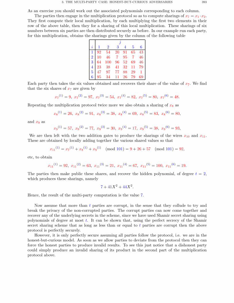
3. THE MULTI-PARTY CASE: HONEST-BUT-CURIOUS ADVERSARIES 393
As an exercise you should work out the associated polynomials corresponding to each column.The parties then engage in the multiplication protocol so as to compute sharings of x7 = x1 ·x2.
They first compute their local multiplication, by each multiplying the first two elements in theirrow of the above table, then they for a sharing of this local multiplication. These sharings of sixnumbers between six parties are then distributed securely as before. In our example run each party,for this multiplication, obtains the sharings given by the column of the following table
ji 1 2 3 4 5 61 92 54 20 91 65 432 10 46 7 95 7 463 64 100 96 52 69 464 23 38 41 32 11 795 47 97 77 88 29 16 95 34 11 26 79 69
Each party then takes the six values obtained and recovers their share of the value of x7. We findthat the six shares of x7 are given by
x7(1) = 9, x7
(2) = 97, x7(3) = 54, x7
(4) = 82, x7(5) = 80, x7
(6) = 48.
Repeating the multiplication protocol twice more we also obtain a sharing of x8 as
x8(1) = 26, x8
(2) = 91, x8(3) = 38, x8
(4) = 69, x8(5) = 83, x8
(6) = 80,
and x9 as
x9(1) = 57, x9
(2) = 77, x9(3) = 30, x9
(4) = 17, x9(5) = 38, x9
(6) = 93,
We are then left with the two addition gates to produce the sharings of the wires x10 and x11.These are obtained by locally adding together the various shared values so that
x11(1) = x7
(1) + x8(1) + x9
(1) (mod 101) = 9 + 26 + 57 (mod 101) = 92,
etc, to obtain
x11(1) = 92, x11
(2) = 63, x11(3) = 21, x11
(4) = 67, x11(5) = 100, x11
(6) = 19.
The parties then make public these shares, and recover the hidden polynomial, of degree t = 2,which produces these sharings, namely
7 + 41X2 + 44X2.
Hence, the result of the multi-party computation is the value 7.
Now assume that more than t parties are corrupt, in the sense that they collude to try andbreak the privacy of the non-corrupted parties. The corrupt parties can now come together andrecover any of the underlying secrets in the scheme, since we have used Shamir secret sharing usingpolynomials of degree at most t. It can be shown that, using the perfect secrecy of the Shamirsecret sharing scheme that as long as less than or equal to t parties are corrupt then the aboveprotocol is perfectly securely.
However, it is only perfectly secure assuming all parties follow the protocol, i.e. we are in thehonest-but-curious model. As soon as we allow parties to deviate from the protocol then they canforce the honest parties to produce invalid results. To see this just notice that a dishonest partycould simply produce an invalid sharing of its product in the second part of the multiplicationprotocol above.
394 26. SECURE MULTI-PARTY COMPUTATION
4. The Multi-Party Case: Malicious Adversaries
To produce a scheme which is secure against such active adversaries we need to force all partiesto either follow the protocol, or we should be able to recover from errors which malicious partiesintroduce introduce into the protocol. It is the second of these two approaches which we shall followin this section, by using the error correction properties of the Shamir secret sharing scheme.
As already remarked the above protocol is not secure against malicious adversaries, due to theability of an attacker to make the multiplication protocol output an invalid answer. To make theabove protocol secure against malicious adversaries we make use of various properties of the Shamirsecret sharing scheme.
The protocol runs in two stages: The preprocessing stage does not involve any of the secretinputs of the parties, it purely depends on the number of multiplication gates in the circuit. In themain phase of the protocol the circuit is evaluated as in the previous section, but using a slightlydifferent multiplication protocol. Malicious parties can force the preprocessing stage to fail, howeverif it completes then the honest parties will be able to evaluate the circuit as required.
The preprocessing phase runs as follows. First using the techniques from Chapter 23 a pseu-dorandom secret sharing scheme, PRSS, and a pseudorandom zero sharing scheme, PRZS, are setup. Then for each multiplication gate in the circuit we compute a random triple of sharings a(i),b(i) and c(i) such that c = a · b. This is done as follows:
• Using PRSS generate two random sharings, a(i) and b(i), of degree t.• Using PRSS generate another random sharing r(i) of degree t.• Using PRZS generate a sharing z(i), of degree 2 · t of zero.• Each player then locally computes
s(i) = a(i) · b(i) − r(i) + z(i).
Note this local computation will produce a degree 2 · t sharing of the value s = a · b− r.• Then the players broadcast their values s(i) and try to recover s. This can be done
always using the error correction properties of Reed–Solomon codes assuming the numberof malicious parties is bounded by n/3.
• Now the players locally compute the shares c(i) from c(i) = s+ r(i).
Assuming the above preprocessing phase completes successfully all we need do is specify howthe parties implement a Mult in the presence of malicious adversaries. We assume the inputs to themultiplication gate are given by x(i) and y(i) and we wish to compute a sharing z(i) of the producez = x · y. From the preprocessing stage, the parties also have for each gate, a triple of shares a(i),b(i) and c(i) such that c = a · b. The protocol for the multiplication is then as follows:
• Compute locally, and then broadcast, the values d(i) = x(i) − a(i) and e(i) = y(i) − b(i)
• Reconstruct the values of d = x− a and d = y − b.• Locally compute the shares
z(i) = d · e+ d · b(i) + e · a(i) + c(i).
Note that the reconstruction in the second step can be completed as long as there are at mostt < n/3 malicious parties. The computation in the last step recovers the valid shares due to thelinear nature of the Shamir secret sharing scheme and the underlying equation
d · e+ d · b+ e · a+ c = (x− a) · (y − b) + (x− a) · b+ (y − b) · a+ c
= ((x− a) + a) · ((y − b) + b)= x · y = z.
Further Reading 395
Chapter Summary
• We have explained how to perform two party secure computation in the precense of honest-but-curious adversaries using Yao’s garbled circuit construction.
• For the many party case we have presented a protocol based on evaluating arithmetic, asopposed to binary, circuits which is based on Shamir secret sharing.
• The main issue with this latter protocol is how to evaluate the multiplication gates. Wepresented two methods: The first, simpler, method is applicable when one is only dealingwith honest-but-curious adversaries, the second, more involved, method is for the case ofmalicious adversaries.
Further Reading
The original presentation of Yao’s idea appears in FOCS 1986, It can be transformed into ascheme for malicious adversaries using a general technique of Goldreich et. al. The discussion ofthe secret sharing based solution for the honest and malicious cases closely follows the treatmentin Damgard et. al.
I. Damgard, M. Geisler, M. Kroigaard and J.B. Nielsen. Asynchronous multiparty computation:Theory and implementation IACR e-print eprint.iacr.org/2008/415.
O. Goldreich, S. Micali and A. Wigderson. How to play any mental game. In Symposium on Theoryof Computing – STOC 1987, ACM, 218–229, 1987.
A.C. Yao. How to generate and exchange secrets. In Foundations of Computer Science – FOCS1986, IEEE, 162–167, 1986.

APPENDIX A
Basic Mathematical Terminology
This appendix is presented as a series of notes which summarizes most of the mathematicalterminology needed in this book. In this appendix we present the material in a more formal mannerthan we did in Chapter 1 and the rest of the book.
1. Sets
Here we recap on some basic definitions etc. which we list here for completeness.
Definition A.1. For two sets A, B we define the union, intersection, difference and cartesianproduct by
A ∪B = {x : x ∈ A or x ∈ B},A ∩B = {x : x ∈ A and x ∈ B},A \B = {x : x ∈ A and x �∈ B},A×B = {(x, y) : x ∈ A and y ∈ B}.
The statement A ⊂ B means thatx ∈ A⇒ x ∈ B.
Using these definitions one can prove in a standard way all the basic results of set theory thatone shows in school using Venn diagrams. For example
Lemma A.2. If A ⊂ B and B ⊂ C then A ⊂ C.
Proof. Let x be an element of A, we wish to show that x is an element of C. Now as A ⊂ Bwe have that x ∈ B, and as B ⊂ C we then deduce that x ∈ C. �
Notice that this is a proof whereas an argument using Venn diagrams is not a proof. UsingVenn diagrams merely shows you were not clever enough to come up with a picture which provedthe result false.
2. Relations
Next we define relations and some properties that they have. Relations, especially equivalencerelations, play an important part in algebra and it is worth considering them at this stage so it iseasier to understand what is going on later.
Definition A.3. A (binary) relation on a set A is a subset of the Cartesian product A×A.
This we explain with an example:Consider the relationship ‘less than or equal to’ between natural numbers. This obviously gives
us the setLE = {(x, y) : x, y ∈ N, x is less than or equal to y}.
In much the same way every relationship that you have met before can be written in this set-theoretic way. An even better way to put the above is to define the relation less than or equal toto be the set
LE = {(x, y) : x, y ∈ N, x− y �∈ N \ {0}}.397
398 A. BASIC MATHEMATICAL TERMINOLOGY
Obviously this is a very cumbersome notation so for a relation R on a set S we write
x R y
if (x, y) ∈ R, i.e. if we now write ≤ for LE we obtain the usual notation 1 ≤ 2 etc.Relations which are of interest in mathematics usually satisfy one or more of the following four
properties:
Definition A.4.A relation R on a set S is reflexive if for all x ∈ S we have (x, x) ∈ R.A relation R on a set S is symmetric if (x, y) ∈ R implies that (y, x) ∈ R.A relation R on a set S is anti-symmetric if (x, y) ∈ R and (y, x) ∈ R implies that x = y.A relation R on a set S is transitive if (x, y) ∈ R and (y, z) ∈ R implies that (x, z) ∈ R.
We return to our example of ≤. This relation ≤ is certainly reflexive as x ≤ x for all x ∈ N. Itis not symmetric as x ≤ y does not imply that y ≤ x, however it is anti-symmetric as x ≤ y andy ≤ x imply that x = y. You should note that it is transitive as well.
Relations like ≤ occur so frequently that we give them a name:
Definition A.5. A relation which is reflexive, transitive and anti-symmetric is called a partialorder relation.
Definition A.6. A relation which is transitive and anti-symmetric and which for all x, y wehave either (x, y) ∈ R or (y, x) ∈ R is called a total order relation.
Another important type of relationship is that of an equivalence relation:
Definition A.7. A relation which is reflexive, symmetric and transitive is called an equivalencerelation.
The obvious example of N and the relation ‘is equal to’ is an equivalence relation and hence givesthis type of relation its name. One of the major problems in any science is that of classification ofsets of objects. This amounts to placing the objects into mutually disjoint subsets. An equivalencerelation allows us to place equivalent elements into disjoint subsets. Each of these subsets is calledan equivalence class. If the properties we are interested in are constant over each equivalence classthen we may as well restrict our attention to the equivalence classes themselves. This often leads togreater understanding. In the jargon this process is called factoring out by the equivalence relation.It occurs frequently in algebra to define new objects from old, e.g. quotient groups. The followingexample is probably the most familiar being a description of modular arithmetic:
Let m be a fixed positive integer. Consider the equivalence relation on Z which says x is relatedto y if (x − y) is divisible by m. This is an equivalence relation, which you should check. Theequivalence classes we denote by
0 = {. . . ,−2m,−m, 0,m, 2m, . . .},1 = {. . . ,−2m+ 1,−m+ 1, 1,m + 1, 2m+ 1, . . .},
. . . . . .
m− 1 = {. . . ,−m− 1,−1,m− 1, 2m − 1, 3m− 1, . . .}.Note that there are m distinct equivalence classes, one for each of the possible remainders
on division by m. The classes are often called the residue classes modulo m. The resulting set{0, . . . ,m− 1} is often denoted by Z/mZ as we have divided out by all multiples of m. If m is aprime number, say p, then the resulting set is often denoted Fp as the resulting object is a field.
3. FUNCTIONS 399
3. Functions
We give two definitions of functions; the first is wordy and is easier to get hold of, the secondis set-theoretic.
Definition A.8. A function is a rule which maps the elements of one set, the domain, withthose of another, the codomain. Each element in the domain must map to one and only one elementin the codomain.
The point here is that the function is not just the rule, e.g. f(x) = x2, but also the two setsthat one is using. A few examples will suffice.
(1) The rule f(x) =√x is not a function from R to R since the square root of a negative
number is not in R. It is also not a function from R≥0 to R since every element of thedomain has two square roots in the codomain. But it is a function from R≥0 to R≥0.
(2) The rule f(x) = 1/x is not a function from R to R but it is a function from R \ {0} to R.(3) Note not every element of the codomain need have an element mapping to it. Hence, the
rule f(x) = x2 taking elements of R to elements of R is a function.Our definition of a function is unsatisfactory as it would also require a definition of what a rule is.In keeping with the spirit of everything else we have done we give a set-theoretic description.
Definition A.9. A function from the set A to the set B is a subset F of A×B such that:(1) If (x, y) ∈ F and (x, z) ∈ F then y = z.(2) For all x ∈ A there exists a y ∈ B such that (x, y) ∈ F .
The set A is called the domain, the set B the codomain. The first condition means that eachelement in the domain maps to at most one element in the codomain. The second condition meansthat each element of the domain maps to at least one element in the codomain. Given a functionf from A to B and an element x of A then we denote by f(x) the unique element in B such that(x, f(x)) ∈ f .
One can compose functions, if the definitions make sense. Say one has a function f from A to Band a function g from B to C then the function g ◦ f is the function with domain A and codomainC consisting of the elements (x, g(f(x))).
Lemma A.10. Let f be a function from A to B, let g be a function from B to C and h be afunction from C to D, then we have
h ◦ (g ◦ f) = (h ◦ g) ◦ f.Proof. Let (a, d) belong to (h ◦ g) ◦ f . Then their exists an (a, b) ∈ f and a (b, d) ∈ (h ◦ g)
for some b ∈ B, by definition of composition of functions. Again by definition there exists a c ∈ Csuch that (b, c) ∈ g and (c, d) ∈ h. Hence (a, c) ∈ (g ◦ f), which shows (a, d) ∈ h ◦ (g ◦ f). Hence
(h ◦ g) ◦ f ⊂ h ◦ (g ◦ f).
Similarly one can show the other inclusion. �One function, the identity function, is particularly important:
Definition A.11. The identity function idA on a set A is the set {(x, x) : x ∈ A}.Lemma A.12. For any function f from A to B we have
f ◦ idA = idB ◦ f = f.
Proof. Let x be an element of A, then
(f ◦ idA)(x) = f(idA(x)) = f(x) = idB(f(x)) = (idB ◦ f)(x).
�
400 A. BASIC MATHEMATICAL TERMINOLOGY
Two properties that we shall use all the time are the following:
Definition A.13.A function f from A to B is said to be injective (or 1:1) if for any two elements, x, y of A withf(x) = f(y) we have x = y.A function f from A to B is said to be surjective (or onto) if for every element b ∈ B there existsan element a ∈ A such that f(a) = b.
A function which is both injective and surjective is called bijective (or a 1:1 correspondence).We shall now give some examples.
(1) The function from R to R given by f(x) = x+ 2 is bijective.(2) The function from N to N given by f(x) = x + 2 is injective but not surjective as the
elements {0, 1} are not the image of anything.(3) The function from R to R≥0 given by f(x) = x2 is surjective as every non-negative real
number has a square root in R but it is not injective as if x2 = y2 then we could havex = −y.
The following gives us a good reason to study bijective functions.
Lemma A.14. A function f : A→ B is bijective if and only if there exists a function g : B → Asuch that f ◦ g and g ◦ f are the identity function.
We leave the proof of this lemma as an exercise. Note, applying this lemma to the resulting gmeans that g is also bijective. Such a function as g in the above lemma is called an inverse of fand is usually denoted f−1. Note that a function only has an inverse if it is bijective.
4. Permutations
We let A be a finite set of cardinality n, without loss of generality we can assume that A ={1, 2, . . . , n}. A bijective function from A to A is called a permutation. The set of all permutationson a set of cardinality n is denoted by Sn.
Suppose A = {1, 2, 3}, then we have the permutation f(1) = 2, f(2) = 3 and f(3) = 1. This isa very cumbersome way to write a permutation. Mathematicians (being lazy people) have inventedthe following notation, the function f above is written as(
1 2 32 3 1
).
What should be noted about this notation (which applies for arbitrary n) is that all the numbersbetween 1 and n occur exactly once on each row. The first row is always given as the numbers 1to n in increasing order. Any such matrix with these properties represents a permutation, and allpermutations can be represented by such a matrix. This leads us to the elementary
Lemma A.15. The cardinality of the set Sn is n!.
Proof. This is a well-known argument. There are n choices for the first element in the secondrow of the above matrix. Then there are n − 1 choices for the second element in the second rowand so on. �
If σ is a permutation on a set S then we usually think of σ acting on the set. So if s ∈ S thenwe write
sσ
for the action of σ on the element s.
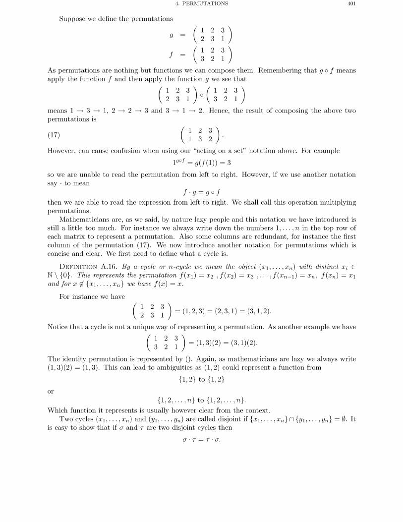
4. PERMUTATIONS 401
Suppose we define the permutations
g =(
1 2 32 3 1
)
f =(
1 2 33 2 1
)As permutations are nothing but functions we can compose them. Remembering that g ◦ f meansapply the function f and then apply the function g we see that(
1 2 32 3 1
)◦(
1 2 33 2 1
)means 1 → 3 → 1, 2 → 2 → 3 and 3 → 1 → 2. Hence, the result of composing the above twopermutations is
(17)(
1 2 31 3 2
).
However, can cause confusion when using our “acting on a set” notation above. For example
1g◦f = g(f(1)) = 3
so we are unable to read the permutation from left to right. However, if we use another notationsay · to mean
f · g = g ◦ fthen we are able to read the expression from left to right. We shall call this operation multiplyingpermutations.
Mathematicians are, as we said, by nature lazy people and this notation we have introduced isstill a little too much. For instance we always write down the numbers 1, . . . , n in the top row ofeach matrix to represent a permutation. Also some columns are redundant, for instance the firstcolumn of the permutation (17). We now introduce another notation for permutations which isconcise and clear. We first need to define what a cycle is.
Definition A.16. By a cycle or n-cycle we mean the object (x1, . . . , xn) with distinct xi ∈N \ {0}. This represents the permutation f(x1) = x2 , f(x2) = x3 , . . . , f(xn−1) = xn, f(xn) = x1
and for x �∈ {x1, . . . , xn} we have f(x) = x.
For instance we have (1 2 32 3 1
)= (1, 2, 3) = (2, 3, 1) = (3, 1, 2).
Notice that a cycle is not a unique way of representing a permutation. As another example we have(1 2 33 2 1
)= (1, 3)(2) = (3, 1)(2).
The identity permutation is represented by (). Again, as mathematicians are lazy we always write(1, 3)(2) = (1, 3). This can lead to ambiguities as (1, 2) could represent a function from
{1, 2} to {1, 2}or
{1, 2, . . . , n} to {1, 2, . . . , n}.Which function it represents is usually however clear from the context.
Two cycles (x1, . . . , xn) and (y1, . . . , yn) are called disjoint if {x1, . . . , xn}∩ {y1, . . . , yn} = ∅. Itis easy to show that if σ and τ are two disjoint cycles then
σ · τ = τ · σ.
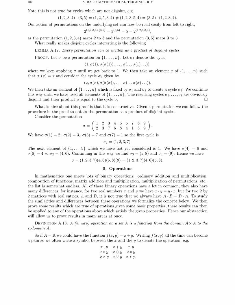
402 A. BASIC MATHEMATICAL TERMINOLOGY
Note this is not true for cycles which are not disjoint, e.g.
(1, 2, 3, 4) · (3, 5) = (1, 2, 5, 3, 4) �= (1, 2, 3, 5, 4) = (3, 5) · (1, 2, 3, 4).Our action of permutations on the underlying set can now be read easily from left to right,
2(1,2,3,4)·(3,5) = 3(3,5) = 5 = 2(1,2,5,3,4),
as the permutation (1, 2, 3, 4) maps 2 to 3 and the permutation (3, 5) maps 3 to 5.What really makes disjoint cycles interesting is the following
Lemma A.17. Every permutation can be written as a product of disjoint cycles.
Proof. Let σ be a permutation on {1, . . . , n}. Let σ1 denote the cycle
(1, σ(1), σ(σ(1)), . . . , σ(. . . σ(1) . . .)),
where we keep applying σ until we get back to 1. We then take an element x of {1, . . . , n} suchthat σ1(x) = x and consider the cycle σ2 given by
(x, σ(x), σ(σ(x)), . . . , σ(. . . σ(x) . . .)).
We then take an element of {1, . . . , n} which is fixed by σ1 and σ2 to create a cycle σ3. We continuethis way until we have used all elements of {1, . . . , n}. The resulting cycles σ1, . . . , σt are obviouslydisjoint and their product is equal to the cycle σ. �
What is nice about this proof is that it is constructive. Given a permutation we can follow theprocedure in the proof to obtain the permutation as a product of disjoint cycles.
Consider the permutation
σ =(
1 2 3 4 5 6 7 8 92 3 7 6 8 4 1 5 9
).
We have σ(1) = 2, σ(2) = 3, σ(3) = 7 and σ(7) = 1 so the first cycle is
σ1 = (1, 2, 3, 7).
The next element of {1, . . . , 9} which we have not yet considered is 4. We have σ(4) = 6 andσ(6) = 4 so σ2 = (4, 6). Continuing in this way we find σ3 = (5, 8) and σ4 = (9). Hence we have
σ = (1, 2, 3, 7)(4, 6)(5, 8)(9) = (1, 2, 3, 7)(4, 6)(5, 8).
5. Operations
In mathematics one meets lots of binary operations: ordinary addition and multiplication,composition of functions, matrix addition and multiplication, multiplication of permutations, etc.,the list is somewhat endless. All of these binary operations have a lot in common, they also havemany differences, for instance, for two real numbers x and y we have x · y = y · x, but for two 2 by2 matrices with real entries, A and B, it is not true that we always have A · B = B · A. To studythe similarities and differences between these operations we formalize the concept below. We thenprove some results which are true of operations given some basic properties, these results can thenbe applied to any of the operations above which satisfy the given properties. Hence our abstractionwill allow us to prove results in many areas at once.
Definition A.18. A (binary) operation on a set A is a function from the domain A×A to thecodomain A.
So if A = R we could have the function f(x, y) = x+y. Writing f(x, y) all the time can becomea pain so we often write a symbol between the x and the y to denote the operation, e.g.
x · y x+ y x yx ◦ y x' y x ( yx ∧ y x ∨ y x � y.
5. OPERATIONS 403
Most often we write x + y and x · y, we refer to the former as additive notation and the latter asmultiplicative notation. One should bear in mind that we may not be actually referring to ordinarymultiplication and addition when we use these terms/notations.
Operations can satisfy various properties:
Definition A.19 (Associative). An operation ( is said to be associative if for all x, y and zwe have
(x ( y) ( z = x ( (y ( z).Operations which are associative include all those examples mentioned above. Non-associative
operations do exist but cryptographers have very little interest in them. Note that for an associativeoperation the expression
w ( x ( y ( zis well defined, as long as we do not move the relative position of any of the terms it does notmatter which operation we carry out first.
Definition A.20 (Commutative). An operation ∨ is said to be commutative if for all x and ywe have
x ∨ y = y ∨ x.Ordinary addition, multiplication and matrix addition is commutative, but multiplication of
matrices and permutations is not.
Definition A.21 (Identity). An operation · on the set A is said to have an identity if thereexists an element e of A such that for all x we have
e · x = x · e = x.
The first thing we notice is that all the example operations above possess an identity, but thatordinary subtraction on the set R does not possess an identity. The following shows that there canbe at most one identity for any given operation.
Lemma A.22. If an identity exists then it is unique. It is then called ‘the’ identity.
Proof. Suppose there are two identities e and e′. As e is an identity we have e · e′ = e′ and ase′ is an identity we have e · e′ = e. Hence, we have e′ = e · e′ = e. �
Usually if we are using an additive notation then we denote the identity by 0 to correspondwith the identity for ordinary addition, and if we are using the multiplicative notation then wedenote the identity by either 1 or e.
Definition A.23 (Inverses). Let + be an operation on a set A with identity 0. Let x ∈ A. Ifthere is a y ∈ A such that
x+ y = y + x = 0then we call y an inverse of x.
In the additive notation it is usual to write the inverse of x as −x. In the multiplicative notationit is usual to write the inverse as x−1.
All elements in R have inverses with respect to ordinary addition. All elements in R exceptzero have inverses with respect to ordinary multiplication. Every permutation has an inverse withrespect to multiplication of permutations. However, only square matrices of non-zero determinanthave inverses with respect to matrix multiplication.
The next result shows that an element can have at most one inverse assuming the operation isassociative.
Lemma A.24. Consider an associative operation on a set A with identity e. Let x ∈ A have aninverse y, then this inverse is unique, we call it ‘the’ inverse.
404 A. BASIC MATHEMATICAL TERMINOLOGY
Proof. Suppose their are two such inverses y and y′ then
y = ye = y(xy′) = (yx)y′ = ey′ = y′.
Note how we used the associativity property above. �We shall assume from now on that all operations we shall encounter are associative. Say one
wishes to perform the same operation over and over again, for example
x ∨ x ∨ x ∨ · · · ∨ x ∨ x.If our operation is written additively then we write for n ∈ N, n · x for x + · · · + x, whilst if ouroperation is written multiplicatively we write xn for x · · · x.
The following result can be proved by induction:
Lemma A.25 (Law of Powers). For any operation ◦ which is associative we have
gm ◦ gn = gm+n, (gm)n = gm·n.
We can extend the notation to all n ∈ Z, if x has an inverse (and the operation an identity),by (−n) · x = n · (−x) and x−n = (x−1)n.
The following lemma is obvious, but often causes problems as it is slightly counter-intuitive.To get it in your brain consider the case of matrices.
Lemma A.26. Consider a set with an associative operation which has an identity, e. If x, y ∈ Gpossess inverses then we have
(1) (x−1)−1 = x.(2) (xy)−1 = y−1x−1.
Proof. For the first we notice
x−1 · x = e = x · x−1.
Hence by definition of inverses the result follows. For the second we have
x · y · (y−1 · x−1) = x · (y · y−1) · x−1 = x · e · x−1 = x · x−1 = e,
and again the result follows by the definition of inverses. �We have the following dictionary to translate between additive and multiplicative notations:
Additive Multiplicativex+ y xy
0 1 or e−x x−1
n · x xn
6. Groups
Definition A.27. A group is a set G with a binary operation ◦ such that(1) ◦ is associative.(2) ◦ has an identity element in G.(3) Every element of G has an inverse.
Note we have not said that the binary operation is closed as this is implicit in our definition ofwhat an operation is. If the operation is also commutative then we say that we have a commutative,or abelian, group.
The following are all groups, as an exercise you should decide on the identity element, what theinverse of each element is, and which groups are abelian.
(1) The integers Z under addition (written Z+).(2) The rationals Q under addition (written Q+).
6. GROUPS 405
(3) The reals R under addition (written R+).(4) The complexes C under addition (written C+).(5) The rationals (excluding zero) Q \ {0} under multiplication (written Q∗).(6) The reals (excluding zero) R \ {0} under multiplication (written R∗).(7) The complexes (excluding zero) C \ {0} under multiplication (written C∗).(8) The set of n vectors over Z,Q, . . . , etc. under vector addition.(9) The set of n × m matrices with integer, rational, real or complex entries under matrix
addition. This set is written Mn×m(Z), etc. however when m = n we write Mn(Z) insteadof Mn×n(Z).
(10) The general linear group (the matrices of non-zero determinant) over the rationals, realsor complexes under matrix multiplication (written GLn(Q), etc.).
(11) The special linear group (the matrices of determinant ±1) over the integers, rationals etc.(written SLn(Z), etc.).
(12) The set of permutations on n elements, written Sn and often called the symmetric groupon n letters.
(13) The set of continuous (differentiable) functions from R to R under pointwise addition.(14) etc.
The list is endless, a group is one of the most basic concepts in mathematics.Not all mathematical objects are however groups. Consider the following list of sets and oper-
ations which are not groups. You should decide why they are not groups.(1) The natural numbers N under ordinary addition or multiplication.(2) The integers Z under subtraction or multiplication.
We now give a number of definitions related to groups.
Definition A.28.The order of a group is the number of elements in the underlying set G and is denoted |G| or #G.The order of an element g ∈ G is the least positive integer n such that gn = e, if such an n existsotherwise we say that g has infinite order.A cyclic group G is a group which has an element g such that each element of G can be writtenin the form gn for some n ∈ Z (in multiplicative notation). If this is the case then one can writeG = 〈g〉 and one says that g is a generator of the group G.
Note, the only element in a group with order one is the identity element and if x is an elementof a group then x and x−1 have the same order.
Lemma A.29. If G = 〈g〉 and g has finite order n then the order of G is n.
Proof. Every element of G can be written as gm for some m ∈ Z, but as g has order n thereare only n distinct such values, as
gn+1 = gn ◦ g = e ◦ g = g.
So the group G has only n elements. �
Let us relate this back to the permutations which we introduced earlier. Recall that the set ofpermutations forms a group under composition. It is easy to see that if σ ∈ Sn is a k-cycle then σhas order k in Sn. One can also easily see that if σ is a product of disjoint cycles then the order ofσ is the least common multiple of the orders of the constituent cycles.
A subset S of G is said to generate G if every element of G can be written as a product ofelements of S. For instance
• the group S3 is generated by the set {(1, 2), (1, 2, 3)},• the group Z+ is generated by the element 1,
406 A. BASIC MATHEMATICAL TERMINOLOGY
• the group Q∗ is generated by the set of prime numbers, it therefore has an infinite numberof generators.
Note that the order of a group says nothing about the number of generators it has.An important set of finite groups which are easy to understand is groups obtained by considering
the integers modulo a number m. Recall that we have Z/mZ = {0, 1, . . . ,m− 1}. This is a groupwith respect to addition, when we take the non-negative remainder after forming the sum of twoelements. It is not a group with respect to multiplication in general, even when we exclude 0. Wecan, however, get around this by setting
(Z/mZ)∗ = {x ∈ Z/mZ : (m,x) = 1}.This latter set is a group with respect to multiplication, when we take the non-negative remainderafter forming the product of two elements. The order of (Z/mZ)∗ is denoted φ(m), the Euler φfunction. This is an important function in the theory of numbers. As an example we have
φ(p) = p− 1,
if p is a prime number. We shall return to this function later.We now turn our attention to subgroups.
Definition A.30. A subgroup H of a group G is a subset of G which is also a group withrespect to the operation of G. We write in this case H < G.
Note that by this definition GLn(R) is not a subgroup of Mn(R), although GLn(R) ⊂ Mn(R).The operation on GLn(R) is matrix multiplication whilst that on Mn(R) is matrix addition.
However we do have the subgroup chains:
Z+ < Q+ < R+ < C+,
Q∗ < R∗ < C∗.
If we also identify x ∈ Z with the diagonal matrix diag(x, . . . , x) then we also have that Z+ is asubgroup of Mn(Z) and so on.
As an important example, consider the set 2Z of even integers, this is a subgroup of Z+. If wewrite Z+ = 1Z, then we have nZ < mZ if and only if m divides n, where
mZ = {. . . ,−2m,−m, 0,m, 2m, . . .}.We hence obtain various chains of subgroups of Z+,
18Z < 6Z < 2Z < Z+,
18Z < 9Z < 3Z < Z+,
18Z < 6Z < 3Z < Z+.
We now show that these are the only such subgroups of Z+.
Lemma A.31. The only subgroups of Z+ are nZ for some positive integer n.
Proof. Let H be a subgroup of Z+. As H is non-empty it must contain an element x and itsinverse −x. Hence H contains at least one positive element n. Let n denote the least such positiveelement of H and let m denote an arbitrary non-zero element of H. By Euclidean division, thereexist q, r ∈ Z with 0 ≤ r < n such that
m = qn+ r.
Hence r ∈ H, by choice of n this must mean r = 0. Therefore all elements of H are of the form nqwhich is what was required. �
So every subgroup of Z+ is an infinite cyclic group. This last lemma combined with the earliersubgroup chains gives us a good definition of what a prime number is.
6. GROUPS 407
Definition A.32. A prime number is a (positive) generator of a non-trivial subgroup of Z+,i.e. H �= Z+ or 0, for which no subgroup of Z+ contains H except Z+ and H itself.
What is good about this definition is that we have not referred to the multiplicative structure ofZ to define the primes. Also it is obvious that neither zero nor one is a prime number. In additionthe above definition allows one to generalize the notion of primality to other settings, for how thisis done consult any standard textbook on abstract algebra.
6.1. Normal Subgroups and Cosets. A normal subgroup is particularly important in thetheory of groups. The name should not be thought of as meaning that these are the subgroupsthat normally arise, the name is a historic accident. To define a normal subgroup we first need todefine what is meant by conjugate elements.
Definition A.33. Two elements x, y of a group G are said to be conjugate if there is an elementg ∈ G such that x = g−1yg.
It is obvious that two conjugate elements have the same order. If N is a subgroup of G wedefine, for any g ∈ G,
g−1Ng = {g−1xg : x ∈ N},which is another subgroup of G, called a conjugate of the subgroup N .
Definition A.34. A subgroup N < G is said to be normal if g−1Ng ⊂ N for all g ∈ G. If thisis the case then we write N �G.
For any group G we have G�G and {e}�G and if G is an abelian group then every subgroupof G is normal. The importance of normal subgroups comes from the fact that these are subgroupsthat we can factor out by. This is related to the cosets of a subgroup which we now go on tointroduce.
Definition A.35. Let G be a group and H < G (H is not necessarily normal). Fix an elementg ∈ G then we define the left coset of H with respect to g to be the set
gH = {gh : h ∈ H}.Similarly we define the right coset of H with respect to g to be the set
Hg = {hg : h ∈ H}.Let H denote a subgroup of G then one can show that the set of all left (or right) cosets of H
in G forms a partition of G, but we leave this to the reader. In addition if a, b ∈ G then aH = bHif and only if a ∈ bH, which is also equivalent to b ∈ aH, a fact which we also leave to the readerto show. Note that we can have two equal cosets aH = bH without having a = b.
What these latter facts show is that if we define the relation RH on the group G with respectto the subgroup H by
(a, b) ∈ RH if and only if a = bh for some h ∈ H,then this relation is an equivalence relation. The equivalence classes are just the left cosets of Hin G.
The number of left cosets of a subgroup H in G we denote by (G : H)L, the number of rightcosets we denote by (G : H)R. We are now in a position to prove the most important theorem ofelementary group theory, namely Lagrange’s Theorem.
Theorem A.36 (Lagrange’s Theorem). Let H be a subgroup of a finite group G then
|G| = (G : H)L · |H|(G : H)R · |H|.
Before we prove this result we state some obvious important corollaries;
408 A. BASIC MATHEMATICAL TERMINOLOGY
Corollary A.37.We have (G : H)L = (G : H)R; this common number we denote by (G : H) and call it the index ofthe subgroup H in G.The order of a subgroup and the index of a subgroup both divide the order of the group.If G is a group of prime order, then G has only the subgroups G and 〈e〉.
We now return to the proof of Lagrange’s Theorem.
Proof. We form the following collection of distinct left cosets of H in G which we defineinductively. Put g1 = e and assume we are given i cosets by g1H, . . . , giH. Now take an elementgi+1 not lying in any of the left cosets gjH for j ≤ i. After a finite number of such steps we haveexhausted elements in the group G. So we have disjoint union of left cosets which cover the wholegroup.
G =⋃
1≤i≤(G:H)L
giH.
We also have for each i, j that |giH| = |gjH|, this follows from the fact that the map
H −→ gHh −→ gh
is a bijective map of sets. Hence
|G| =∑
1≤i≤(G:H)L
|giH| = (G : H)L|H|.
The other equality follows using the same argument. �We can also deduce from the corollaries the following
Lemma A.38. If G is a group of prime order then it is cyclic.
Proof. If g ∈ G is not the identity then 〈g〉 is a subgroup of G of order ≥ 2. But then it musthave order |G| and so G is cyclic. �
We can use Lagrange’s Theorem to write down the subgroups of some small groups. Forexample, consider the group S3 this has order 6 so by Lagrange’s Theorem its subgroups must haveorder 1, 2, 3 or 6. It is easy to see that the only subgroups are therefore:
• one subgroup of order 1; namely 〈(1)〉,• three subgroups of order 2; namely 〈(1, 2)〉, 〈(1, 3)〉 and 〈(2, 3)〉,• one subgroup of order 3; namely 〈(1, 2, 3)〉,• one subgroup of order 6, which is S3 obviously.
6.2. Factor or Quotient Groups. Throughout this subsection let G be a group with anormal subgroup N . The following elementary lemma, whose proof we again leave to the reader,gives us our justification for looking at normal subgroups.
Lemma A.39. Let H < G then the following are equivalent:(1) xH = Hx for all x ∈ G.(2) x−1Hx = H for all x ∈ G.(3) H �G.(4) x−1hx ∈ H for all x ∈ G and h ∈ H.
By G/N we denote the set of left cosets of N , note that these are the same as the right cosetsof N . We note that two cosets, g1N and g2N are equal if and only if g−1
1 g2 ∈ N .We wish to turn G/N into a group, the so-called factor group or quotient group. Let g1N and
g2N denote any two elements of G/N then we define the product of their left cosets to be (g1g2)N .
6. GROUPS 409
We first need to show that this is a well-defined operation, i.e. if we replace g1 by g′1 and g2 byg′2 with g−1
1 g′1 = n1 ∈ N and g−12 g′2 = n2 ∈ N then our product still gives the same coset. In other
words we wish to show(g1g2)N = (g′1g
′2)N.
Now let x ∈ (g1g2)N then x = g1g2n for some n ∈ N . Then x = g′1n−11 g′2n
−12 n. But as G is normal
(left cosets = right cosets) we have n′1−1g′2 = g′2n3 for some n3 ∈ N . Hence
x = g′1g′2n3n
−12 n ∈ g′1g
′2N.
This proves the first inclusion, the other follows similarly. We conclude that our operation on G/Nis well defined. One can also show that if N is an arbitrary subgroup of G and we define theoperation on the cosets above then this is only a well-defined operation if N is a normal subgroupof G.
So we have a well-defined operation on G/N , we now need to show that this operation satisfiesthe axioms of a group:
• As an identity we take eN = N , since for all g ∈ G we have
eN · gN = (eg)N = gN.
• As an inverse of (gN) we take g−1N as
gN.g−1N = (gg−1)N = eN = N.
• Associativity follows from
(g1N)(g2N · g3N) = g1N((g2g3)N) = (g1(g2g3))N
= ((g1g2)g3)N = ((g1g2)N)g3N
= (g1N · g2N)(g3N).
We now present some examples.(1) Let G be an arbitrary finite group of order greater than one, let H be a subgroup of G.
Then H = G and H = {e} are always normal subgroups of G.(2) If H = G then there is only one coset and so we have G/G = {G} is a group of order one.(3) If H = {e} then the cosets of H are the one-element subsets of G. That is G/{e} = {{g} :
g ∈ G}.(4) Put G = S3 and N = {(1), (1, 2, 3), (1, 3, 2)}, then N is a normal subgroup of G. The
cosets of N in G are N and (1, 2)N with
((1, 2)N)2 = (1, 2)2N = (1)N = N.
Hence S3/〈(1, 2, 3)〉 is a cyclic group of order 2.(5) If G is abelian then every subgroup H of G is normal, so one can always form the quotient
group G/H.(6) Since (Z,+) is abelian we have thatmZ is always a normal subgroup. Forming the quotient
group Z/mZ we obtain the group of integers modulo m under addition.
6.3. Homomorphisms. Let G1 and G2 be two groups, we wish to look at the functions fromG1 to G2. Obviously one could look at all such functions, however by doing this we would lose allthe structure that the group laws give us. We restrict ourselves to maps which preserve this grouplaw.
Definition A.40. A homomorphism from a group G1 to a group G2 is a function f withdomain G1 and codomain G2 such that for all x, y ∈ G1 we have
f(x · y) = f(x) · f(y).
410 A. BASIC MATHEMATICAL TERMINOLOGY
Note multiplication on the left is with the operation of the group G1 whilst the multiplicationon the right is with respect to the operation of G2. As examples we have
(1) The identity map idG : G→ G, where idG(g) = g is a group homomorphism.(2) Consider the function R+ → R∗ given by f(x) = ex. This is a homomorphism as for all
x, y ∈ R we haveex+y = exey.
(3) Consider the map from C∗ to R∗ given by f(z) = |z|. This is also a homomorphism.(4) Consider the map from GLn(C) to C∗ given by f(A) = det(A), this is a group homomor-
phism as det(AB) = det(A) · det(B) for any two elements of GLn(C).Two elementary properties of homomorphisms are summarized in the following lemma.
Lemma A.41. Let f : G1 → G2 be a homomorphism of groups, then(1) f(e1) = e2.(2) For all x ∈ G1 we have f(x−1) = (f(x))−1.
Proof. For the first result we have e2f(x) = f(x) = f(e1x) = f(e1)f(x) and so
e2 = f(x)f(x)−1 = f(e1)f(x)f(x)−1 = f(e1)
as required.Now for the second we have
f(x−1)f(x) = f(x−1x) = f(e1) = e2,
so the result follows by definition. �For any homomorphism f from G1 to G2 there are two special subgroups associated with f .
Definition A.42.The kernel of f is the set
Kerf = {x ∈ G1 : f(x) = e2}.The image of f is the set
Imf = {y ∈ G2 : y = f(x), x ∈ G1}.Lemma A.43. Kerf is a normal subgroup of G1.
Proof. We first show that it is a subgroup. It is certainly non-empty as e1 ∈ Kerf as f(e1) =e2. Now if x ∈ Kerf then f(x−1) = f(x)−1 = e−1
2 = e2, hence x−1 ∈ Kerf . Hence to show thatKerf is a subgroup we only have to show that for all x, y ∈ Kerf we have xy−1 ∈ Kerf . But thisis easy as if x, y ∈ Kerf then we have
f(xy−1) = f(x)f(y−1) = e2e2 = e2,
and we are done.We now show that Kerf is in fact a normal subgroup of G1. We need to show that if x ∈ Kerf
then g−1xg ∈ Kerf for all g ∈ G1. So let x ∈ Kerf and let g ∈ G1, then we have
f(g−1xg) = f(g−1)f(x)f(g) = f(g)−1e2f(g) = f(g)−1f(g) = e2,
so we are done. �Lemma A.44. Imf is a subgroup of G2.
Proof. Imf is certainly non-empty as f(e1) = e2. Now suppose y ∈ Imf so there is an x ∈ G2
such that f(x) = y, then y−1 = f(x)−1 = f(x−1) and x−1 ∈ G1 so y−1 ∈ Imf .Now suppose y1, y2 ∈ Imf , hence for some x1, x2 we have
y1y−12 = f(x1)f(x−1
2 ) = f(x1x−12 ).
Hence Imf < G2. �
6. GROUPS 411
It is clear that Imf in some sense measures whether the homomorphism f is surjective as f issurjective if and only if Imf = G2. Actually the set G2/Imf is a better measure of the surjectivityof the function. What we also have is that Kerf measures how far from injective f is, due to thefollowing result.
Lemma A.45. A homomorphism, f , is injective if and only if Kerf = {e1}.Proof. Assume f is injective, then we know that if f(x) = e2 = f(e1) then x = e1 and so
Kerf = {e1}.Now assume that Kerf = {e1} and let x, y ∈ G1 be such that f(x) = f(y). Then
f(xy−1) = f(x)f(y−1) = f(x)f(y)−1 = f(x)f(x)−1 = e2.
So xy−1 ∈ Kerf , but then xy−1 = e1 and so x = y. So f is injective. �
Bijective homomorphisms allow us to categorize groups more effectively, as the following defi-nition elaborates.
Definition A.46. A homomorphism f is said to be an isomorphism if it is bijective. Twogroups are said to be isomorphic if there is an isomorphism between them, in which case we writeG1
∼= G2.
Note this means that isomorphic groups have the same number of elements. Indeed for allintents and purposes one may as well assume that isomorphic groups are equal, since they look thesame up to relabelling of elements.
Isomorphisms satisfy the following properties,
• If f : G1 → G2 and g : G2 → G3 are isomorphisms then g ◦ f is also an isomorphism, i.e.isomorphisms are transitive.
• If f : G1 → G2 is an isomorphism then so is f−1 : G2 → G1, i.e. isomorphisms aresymmetric.
From this we see that the relation ‘is isomorphic to’ is an equivalence relation on the class of allgroups. This justifies our notion of isomorphic being like equal.
Let G1, G2 be two groups, then we define the product group G1 × G2 to be the set G1 × G2
of ordered pairs (g1, g2) with g1 ∈ G1 and g2 ∈ G2. The group operation on G1 × G2 is givencomponentwise:
(g1, g2) ◦ (g′1, g′2) = (g1 ◦ g′1, g2 ◦ g′2).
The first ◦ refers to the group G1 ×G2, the second to the group G1 and the third to the group G2.Some well-known groups can actually be represented as product groups. For example, consider themap
C+ −→ R+ × R+
z −→ (Re(z), Im(z)).
This map is obviously a bijective homomorphism, hence we have C+ ∼= R+ × R+.We now come to a crucial theorem which says that the concept of a quotient group is virtually
equivalent to the concept of a homomorphic image.
Theorem A.47 (First Isomorphism Theorem for Groups). Let f be a homomorphism from agroup G1 to a group G2. Then
G1/Kerf ∼= Imf.
The proof of this result can be found in any introductory text on abstract algebra. Note thatG1/Kerf makes sense as Kerf is a normal subgroup of G.
412 A. BASIC MATHEMATICAL TERMINOLOGY
7. Rings
A ring is an additive finite abelian group with an extra operations, usually denoted by multi-plication, such that the multiplication operation is associative and has an identity element. Theaddition and multiplication operations are linked via the distributive law,
a · (b+ c) = a · b+ a · c = (b+ c) · a.If the multiplication operation is commutative then we say we have a commutative ring.
The following are examples of rings.• integers under addition and multiplication,• polynomials with coefficients in Z, denoted Z[X],• integers modulo a number m, denoted Z/mZ.
Although one can consider subrings they turn out to be not so interesting. Of more interest arethe ideals of the ring, these are additive subgroups I < R such that
i ∈ I and r ∈ R implies i · r ∈ I.
Examples of ideals in a ring are the principal ideals which are those additive subgroups generatedby a single ring element. For example if R = Z then the principal ideals are the ideals mZ, for eachinteger m.
Just as with normal subgroups and groups, where we formed the quotient group, we can withideals and rings form the quotient ring. If we take R = Z and I = mZ for some integer m then thequotient ring is the ring Z/mZ of integers modulo m under addition and multiplication modulo m.This leads us naturally to the Chinese Remainder Theorem.
Theorem A.48 (CRT). Let m = pz11 . . . pztt be the prime factorization of m, then the followingmap is a ring isomorphism
f : Z/mZ −→ Z/pz11 Z × · · · × Z/pztt Z
x −→ (x (mod pz11 ), . . . , x (mod pztt )).
Proof. This can be proved by induction on the number of prime factors of m. We leave thedetails to the interested reader. �
We shall now return to the Euler φ function mentioned earlier. Remember φ(n) denotes theorder of the group Z/nZ∗. We would like to be able to calculate this value easily.
Lemma A.49. Let m = pz11 . . . pztt be the prime factorization of m. Then we have
φ(m) = φ(pz11 ) . . . φ(pztt ).
Proof. This follows from the Chinese Remainder Theorem, as the ring isomorphism
Z/mZ ∼= Z/pz11 Z × · · · × Z/pztt Z
induces a group isomorphism
(Z/mZ)∗ ∼= (Z/pz11 Z)∗ × · · · × (Z/pztt Z)∗.
�To compute the Euler φ function all we now require is:
Lemma A.50. Let p be a prime number, then φ(pe) = pe−1(p− 1).
Proof. There are pe− 1 elements of Z satisfying 1 ≤ k < pe, of these we must eliminate thoseof the form k = rp for some r. But 1 ≤ rp < pe implies 1 ≤ r < pe−1, hence there are pe−1 − 1possible values of r. So we obtain
φ(pe) = (pe − 1) − (pe−1 − 1)
from which the result follows. �
8. FIELDS 413
An ideal I of a ring is called prime if x · y ∈ I implies either x ∈ I or y ∈ I. Notice, the idealsI = mZ of the ring Z are prime if and only if m is plus or minus a prime number.
The prime ideals are special as if we take the quotient of a ring by a prime ideal then we obtaina field. Hence, Z/pZ is a field. This brings us naturally on to the subject of fields.
8. Fields
A field is essentially two abelian groups stuck together using the distributive law. More formally:
Definition A.51. A field is an additive abelian group F , such that F \ {0} also forms anabelian group with respect to another operation (which is usually written multiplicatively). The twooperations, addition and multiplication, are linked via the distributive law:
a · (b+ c) = a · b+ a · c = (b+ c) · a.Many fields that one encounters have infinitely many elements. Every finite field either contains
Q as a subfield, in which case we say it has characteristic zero, or it contains Fp as a subfield inwhich case we say it has characteristic p. The only fields with finitely many elements have pr
elements when p is a prime. We denote such fields by Fpr , for each value of r there is only one suchfield up to isomorphism. Such finite fields are often called Galois fields.
Let F be a field, we denote by F [X] the ring of polynomials in a single variable X withcoefficients in the field F . The set F (X) of rational functions in X is the set of functions of theform
f(X)/g(X),where f(X), g(X) ∈ F [X] and g(X) is not the zero polynomial. The set F (X) is a field withrespect to the obvious addition and multiplication. One should note the difference in the notationof the brackets, F [X] and F (X).
Let f be a polynomial of degree n with coefficients in Fp which is irreducible. Let θ denote aroot of f . Consider the set
Fp(θ) = {a0 + a1θ + · · · + an−1θn−1 : ai ∈ Fp}.
Given two elements of Fp(θ) one adds them componentwise and multiplies them as polynomials inθ but then one takes the remainder of the result on division by f(θ). The set Fp(θ) is a field, thereare field-theoretic isomorphisms
Fpn = Fp(θ) = Fp[X]/(f),
where (f) represents the ideal{f · g : g ∈ Fp[X]}.
To be more concrete let us look at the specific example given by choosing a value of p ≡ 3 (mod 4)and f(X) = X2 + 1. Now since p ≡ 3 (mod 4) the polynomial f is irreducible over Fp[X] and sothe quotient Fp[X]/(f) forms a field, which is isomorphic to Fp2.
Let i denote a root of the polynomial X2 + 1. The field Fp2 = Fp(i) consists of numbers of theform
a+ bi
where a and b are integers modulo p. We add such numbers as
(a+ bi) + (c+ di) = (a+ c) + (b+ d)i.
We multiply such numbers as
(a+ bi)(c+ di) = (ac+ (ad+ bc)i+ bdi2) = (ac− bd) + (ad+ bc)i.
Here is another example. Let θ denote a root of the polynomial x3 + 2, then an element of
F73 = F7(θ)
414 A. BASIC MATHEMATICAL TERMINOLOGY
can be represented bya+ bθ + cθ2.
Multiplication of two such elements gives
(a+ bθ + cθ2)(a′ + b′θ + c′θ2) = aa′ + θ(a′b+ b′a) + θ2(ac′ + bb′ + ca′)
+ θ3(bc′ + cb′) + cc′θ4
= (aa′ − 2bc′ − 2cb′) + θ(a′b+ b′a− 2cc′)
+ θ2(ac′ + bb′ + ca′).
9. Vector Spaces
Definition A.52. Given a field K a vector space (or a K-vector space) V is an abelian group(also denoted V ) and an external operation K×V → V (called scalar multiplication) which satisfiesthe following axioms: For all λ, μ ∈ K and all x, y ∈ V we have
(1) λ(μx) = (λμ)x.(2) (λ+ μ)x = λx+ μx.(3) 1Kx = x.(4) λ(x+ y) = λx+ λy.
One often calls the elements of V the vectors and the elements of K the scalars. Note that weare not allowed to multiply or divide two vectors. We shall start with some examples:
• For a given field K and an integer n ≥ 1, let V = Kn = K×· · ·×K be the n-fold Cartesianproduct. This is a vector space over K with respect to the usual addition of vectors andmultiplication by scalars. A special case of n = 1 shows that any field is a vector spaceover itself. When K = R and n = 2 we obtain the familiar system of geometric vectorsin the plane. When n = 3 and K = R we obtain 3-dimensional vectors. Hence you canalready see the power of vector spaces as they allow us to consider n-dimensional space ina concrete way.
• Let K be a field and consider the set of polynomials over K, namely K[X]. This is avector space with respect to addition of polynomials and multiplication by elements of K.
• Let K be a field and E any set at all. Define V to be the set of functions f : E → K.Given f, g ∈ V and λ ∈ K one can define the sum f + g and scalar product λf via
(f + g)(x) = f(x) + g(x) and (λf)(x) = λf(x).
We leave the reader the simple task to check that this is a vector space.• The set of all continuous functions f : R → R is a vector space over R. This follows from
the fact that if f and g are continuous then so is f + g and λf for any λ ∈ R. Similarlythe set of all differentiable functions f : R → R also forms a vector space.
9.1. Vector Sub-spaces. Let V be a K-vector space and let W be a subset of V . W is saidto be a vector subspace (or just subspace) of V if
(1) W is a subgroup of V with respect to addition.(2) W is closed under scalar multiplication.
By this last condition we mean λx ∈ W for all x ∈ W and all λ ∈ K. What this means is that avector subspace is a subset of V which is also a vector space with respect to the same addition andmultiplication laws as are on V . There are always two trivial subspaces of a space, namely {0} andV itself. Here are some more examples:
• Let V = Kn and W = {(ξ1, . . . , ξn) ∈ Kn : ξn = 0}.• Let V = Kn and W = {(ξ1, . . . , ξn) ∈ Kn : ξ1 + · · · + ξn = 0}.• V = K[X] and W = {f ∈ K[X] : f = 0 or deg f ≤ 10}.
9. VECTOR SPACES 415
• C is a natural vector space over Q, and R is a vector subspace of C.• Let V denote the set of all continuous functions from R to R and W the set of all differ-
entiable functions from R to R. Then W is a vector subspace of V .
9.2. Properties of Elements of Vector Spaces. Before we go any further we need to definecertain properties which sets of elements of vector spaces can possess. For the following definitionslet V be a K-vector space and let x1, . . . , xn and x denote elements of V .
Definition A.53.x is said to be a linear combination of x1, . . . , xn if there exists scalars λi ∈ K such that
x = λ1x1 + · · · + λnxn.
The elements x1, . . . , xn are said to be linearly independent if the relation
λ1x1 + · · · + λnxn = 0
implies that λ1 = · · · = λn = 0. If x1, . . . , xn are not linearly independent then they are said to belinearly dependent.A subset A of a vector space is linearly independent or free if whenever x1, . . . , xn are finitely manyelements of A, they are linearly independent.A subset A of a vector space V is said to span (or generate) V if every element of V is a linearcombination of finitely many elements from A.If there exists a finite set of vectors spanning V then we say that V is finite-dimensional.
We now give some examples of the last concept.
• The vector space V = Kn is finite-dimensional. For let
ei = (0, . . . , 0, 1, 0, . . . , 0)
be the n-tuple with 1 in the ith-place and 0 elsewhere. Then V is spanned by the vectorse1, . . . , en. Note the analogy with the geometric plane.
• C is a finite-dimensional vector space over R, and {1,√−1} is a spanning set.• R and C are not finite-dimensional vector spaces over Q. This is obvious since Q has
countably many elements, any finite-dimensional subspace over Q will also have countablymany elements. However it is a basic result in analysis that both R and C have uncountablymany elements.
Now some examples about linear independence:
• In the vector space V = Kn the n-vectors e1, . . . , en defined earlier are linearly indepen-dent.
• In the vector space R3 the vectors x1 = (1, 2, 3), x2 = (−1, 0, 4) and x3 = (2, 5,−1) arelinearly independent.
• On the other hand, the vectors y1 = (2, 4,−3), y2 = (1, 1, 2) and y3 = (2, 8,−17) arelinearly dependent as we have 3y1 − 4y2 − y3 = 0.
• In the vector space (and ring) K[X] over the field K the infinite set of vectors
{1,X,X2,X3, . . .}is linearly independent.
9.3. Dimension and Bases.
Definition A.54. A subset A of a vector space V which is linearly independent and spans thewhole of V is called a basis.
416 A. BASIC MATHEMATICAL TERMINOLOGY
Given a basis then each element in V can be written in a unique way: for if x1, . . . , xn is abasis and suppose that we can write x as a linear combination of the xi in two ways i.e. x =λ1x1 + · · · + λnxn and x = μ1x1 + · · · + μnxn. Then we have
0 = x− x = (λ1 − μ1)x1 + · · · + (λn − μn)xn
and as the xi are linearly independent we obtain λi − μi = 0, i.e. λi = μi.We have the following examples.
• The vectors e1, . . . , en of Kn introduced earlier form a basis of Kn. This basis is calledthe standard basis of Kn.
• The set {1, i} is a basis of the vector space C over R.• The infinite set {1,X,X2,X2, . . .} is a basis of the vector space K[X].
By way of terminology we call the vector space V = {0} the trivial or zero vector space. Allother vector spaces are called non-zero. To make the statements of the following theorems easierwe shall say that the zero vector space has the basis set ∅.
Theorem A.55. Let V be a finite-dimensional vector space over a field K. Let C be a finitesubset of V which spans V and let A be a subset of C which is linearly independent. Then V hasa basis, B, such that A ⊂ B ⊂ C.
Proof. We can assume that V is non-zero. Consider the collection of all subsets of C whichare linearly independent and contain A. Certainly such subsets exist since A is itself an example.So choose one such subset B with as many elements as possible. By construction B is linearlyindependent. We now show that B spans V .
Since C spans V we only have to show that every element x ∈ C is a linear combination ofelements of B. This is trivial when x ∈ B so assume that x �∈ B. Then B′ = B ∪ {x} is a subsetof C larger than B, whence B′ is linearly dependent, by choice of B. If x1, . . . , xr are the distinctelements of B this means that there is a linear relation
λ1x1 + · · · + λrxr + λx = 0,
in which not all the scalars, λi, λ, are zero. In fact λ �= 0. So we may rearrange to express x as alinear combination of elements of B, as λ has an inverse in K. �
Corollary A.56. Every finite-dimensional vector space, V , has a basis.
Proof. We can assume that V is non-zero. Let C denote a finite spanning set of V and letA = ∅ and then apply the above theorem. �
The last theorem and its corollary are true if we drop the assumption of finite dimensional.However then we require much more deep machinery to prove the result. The following result iscrucial to the study of vector spaces as it allows us to define the dimension of a vector space. Oneshould think of dimension of a vector space as the same as dimension of the 2-D or 3-D space oneis used to.
Theorem A.57. Suppose a vector space V contains a spanning set of m elements and a linearlyindependent set of n elements. Then m ≥ n.
Proof. Let A = {x1, . . . , xm} span V , and let B = {y1, . . . , yn} be linearly independent andsuppose that m < n. Hence we wish to derive a contradiction.
We successively replace the xs by the ys, as follows. Since A spans V , there exists scalarsλ1, . . . , λm such that
y1 = λ1x1 + · · · + λmxm.
At least one of the scalars, say λ1, is non-zero and we may express x1 in terms of y1 and x2, . . . , xm.It is then clear that A1 = {y1, x2, . . . , xm} spans V .
9. VECTOR SPACES 417
We repeat the process m times and conclude that Am = {y1, . . . , ym} spans V . (One canformally dress this up as induction if one wants to be precise, which we will not bother with.)
By hypothesis m < n and so Am is not the whole of B and ym+1 is a linear combination ofy1, . . . , ym, as Am spans V . This contradicts the fact that B is linearly independent. �
Let V be a finite-dimensional vector space. Suppose A is a basis of m elements and B a basisof n elements. By applying the above theorem twice (once to A and B and once to B and A) wededuce that m = n. From this we conclude the following theorem.
Theorem A.58. Let V be a finite-dimensional vector space. Then all bases of V have the samenumber of elements, we call this number the dimension of V (written dimV ).
It is clear that dimKn = n. This agrees with our intuition that a vector with n components livesin an n-dimensional world, and that dimR3 = 3. Note when referring to dimension we sometimesneed to be clear about the field of scalars. If we wish to emphasise the field of scalars we writedimK V . This can be important, for example if we consider the complex numbers we have
dimC C = 1, dimR C = 2, dimQ C = ∞.
The following results are left as exercises.
Theorem A.59. If V is a (non-zero) finite-dimensional vector space, of dimension n, then(1) Given any linearly independent subset A of V , there exists a basis B such that A ⊂ B.(2) Given any spanning set C of V , there exists a basis B such that B ⊂ C.(3) Every linearly independent set in V has ≤ n elements.(4) If a linearly independent set has exactly n elements then it is a basis.(5) Every spanning set has ≥ n elements.(6) If a spanning set has exactly n elements then it is a basis.
Theorem A.60. Let W be a subspace of a finite-dimensional vector space V . Then dimW ≤dimV , with equality holding if and only if W = V .

Index
A5/1, 118, 119A5/2, 118Abadi, 148abelian group, 4, 23, 26, 28, 203, 407, 412–414access structure, 349–351active attack, 91adaptive chosen ciphertext attack, 291–293Adleman, 189, 199, 221Adleman–Huang algorithm, 189, 312AES, 124, 131affine point, 24algebraic normal form, 115alternating step generator, 117anomalous, 29, 216ANSI, 126anti-symmetric, 398arithmetic circuit, 386, 390ASN.1, 263associative, 4, 403, 404, 412asymmetric cryptosystems, 37Atlantic City algorithm, 311authenticated key exchange, 231automorphism, 9avalanche affect, 156
Baby-Step/Giant-Step, 206–209, 226BAN logic, 148–151basis, 276, 277, 415basis matrix, 276, 277Baudot code, 96–98, 106Bayes’ Theorem, 20, 82Bellare, 324, 335Berlekamp–Massey algorithm, 115Berlekamp–Welch algorithm, 357–359Bertrand, 57, 62bigrams, 38bijective, 400, 411binary circuit, 386, 387, 390binary Euclidean algorithm, 12, 246, 248binary exponentiation, 236, 237binding, 258, 364–366birthday paradox, 21, 154, 209bit security, 308block cipher, 41, 44, 123, 125, 131, 134–137, 161Bombe, 56, 65–69, 71–73Boneh, 267, 283, 284
BPP, 312Burrows, 148
CA, 258, 262Caesar cipher, 39Carmichael numbers, 187cartesian product, 397CBC Mode, 134, 136, 138, 161, 330, 331CBC-MAC, 161, 162CCA, 293, 330CCA1, 291CCA2, 291, 293certificate authority, 258, 266, 360certificate chains, 260Certificate Revocation List, 260CFB Mode, 135, 137, 138characteristic, 7, 9, 24, 26, 29–33, 248, 413Chaum–Pedersen protocol, 377Chinese Remainder Theorem, 3, 10, 13, 14, 18, 22,
171, 177, 181, 203, 204, 206, 240, 251, 282, 285,286, 296, 412
chord-tangent process, 25, 26chosen ciphertext attack, 91, 173, 179, 291, 296chosen plaintext attack, 47, 91, 173, 179, 291cillies, 58cipher, 37ciphertext, 37closed, 4co-NP, 303co-P, 302, 303co-RP, 312Cocks, 167coding theory, 353codomain, 317, 399collision resistant, 154, 155Colossus, 106, 107commitment, 364commitment scheme, 364–367, 379commutative, 4, 403, 404, 412commutative ring, 412completeness, 373compression function, 155, 156computational zero-knowledge, 373computationally secure, 77, 364concealing, 364–366conditional entropy, 86
419

420 INDEX
conditional probability, 20, 79, 86conjugate, 407connection polynomial, 110continued fraction, 273–275, 279Coppersmith, 279, 283Coppersmith’s Theorem, 281–285coprime, 6correlation attack, 116, 117coset, 407, 408Couveignes, 200CPA, 291, 330Cramer, 332, 333, 337, 341, 342, 378Cramer–Shoup encryption scheme, 342–344Cramer–Shoup signature scheme, 341, 342crib, 58CRL, 260cross-certification, 259CRT, 13, 14CTR Mode, 135, 138cycle, 401cyclic group, 5, 405CZK, 374
Daemen, 131Damgard, 378data integrity, 160, 161Davies–Meyer hash, 159DDH, 170, 171, 294, 295, 310, 311, 316, 322, 343, 344DEA, 126decipherment, 37decision Diffie–Hellman, 170, 171, 294decision problem, 301, 302decryption, 37DEM, 160, 329, 331–334DES, 47, 78, 123–129, 131, 132, 134, 141, 161, 163,
262DHAES, 335DHIES, 324, 333–336, 367difference, 397differential cryptanalysis, 124, 126Diffie, 167, 219, 221Diffie–Hellman Key Exchange, 219Diffie–Hellman problem, 170, 171, 179, 220, 294, 343Diffie–Hellman protocol, 220, 221, 231, 232, 262digital certificate, 258–261, 263digital signature, 222Digital Signature Algorithm, 224Digital Signature Standard, 224dimension, 417discrete logarithm, 5discrete logarithm problem, 169, 170, 178, 194,
203–216, 219, 224, 226discriminant, 24, 277disjoint, 401disjunctive normal form, 351distributive, 4, 412, 413DLOG, 231domain, 399domain parameters, 178, 220, 225, 342
DSA, 219, 224–229, 231, 233, 235, 240, 252, 261, 266,267, 284, 317–320, 324, 340
DSS, 224Durfee, 283, 284
EC-DH, 220, 221EC-DSA, 224, 226, 227, 231, 233, 266, 317, 319, 320ECB Mode, 134–136, 138, 139, 223ECPP, 189, 312ElGamal, 367ElGamal encryption, 78, 167, 178, 179, 185, 225, 235,
289, 293–296, 299, 322–324, 327, 335, 343, 344,366
elliptic curve, 23–33, 169, 178, 185, 189, 215, 216,220, 221, 224, 226–228, 231, 239, 241, 248
Elliptic Curve Method, 168Ellis, 167encipherment, 37encryption, 37Enigma, 49–54, 56, 57, 61, 63, 65–67, 70, 71, 73, 96entropy, 84–88, 142equivalence class, 398equivalence relation, 23, 25, 397, 398, 411error-correcting code, 353Euclidean algorithm, 10–12, 248, 283Euclidean division, 11, 243, 406Euler φ function, 6, 406, 412exhaustive search, 94existential forgery, 298, 315extended Euclidean algorithm, 12, 13, 31, 169, 172,
173
factor group, 408factorbase, 194factoring, 168, 169, 171, 224feedback shift register, 109Feistel, 325Feistel cipher, 125, 126, 131female, 63, 64Fermat test, 187, 188, 312Fermat’s Little Theorem, 7, 186, 192Fiat–Shamir heuristic, 376field, 6, 131, 413Filter generator, 117finite field, 7–9, 23, 28–31, 111, 169, 178, 185, 189,
205, 207, 214, 215, 220, 224, 228, 231, 239, 248,251, 413
finite-dimensional, 415fixed field, 9flexible RSA problem, 340Floyd’s cycle finding algorithm, 209–211forking lemma, 317forward secrecy, 219Franklin, 267Franklin–Reiter attack, 282, 283frequency analysis, 40Frobenius endomorphism, 29Frobenius map, 9, 29Fujisaki, 327, 333

INDEX 421
full domain hash, 320function, 399
Galois field, 9, 413Gap-Diffie–Hellman problem, 336garbled circuit, 386–389Gauss, 185gcd, 5, 11, 12GCHQ, 167Geffe generator, 115–117generator, 5, 405Gennaro, 340GHR signature scheme, 340, 341Gillogly, 73Goldwasser, 189, 296, 297, 340Goldwasser–Micali encryption, 296, 297Gram–Schmidt, 276–279graph, 301graph isomorphism, 371, 372, 374greatest common divisor, 5, 8, 10, 45group, 4, 186, 203, 404–411GSM, 118
Halevi, 340Hamming weight, 236hard predicate, 308hash function, 153–162, 219, 223, 224, 228, 230, 293,
298, 316–326, 376Hasse’s Theorem, 215Hastad, 282Hastad’s attack, 282, 283HDH, 334Hellman, 167, 203, 219, 221, 304hiding, 364HMAC, 161homomorphic property, 294homomorphism, 204, 409–411honest-but-curious, 385, 386, 393honest-verifier, 374, 375Howgrave-Graham, 279Huang, 189hybrid cipher, 329, 332, 333hyperelliptic curve, 189
IDEA, 261ideal, 198, 199, 412identity, 403, 404identity based encryption, 267identity based signature, 267identity certificate, 258image, 410independent, 20index, 408index of Coincidence, 73index-calculus, 214indian exponentiation, 237indistinguishability of encryptions, 290, 293, 330information theoretic security, 78, 290, 364injective, 81, 294, 400, 411inner product, 275
intersection, 397inverse, 400, 403, 404IP, 373, 374irreducible, 8ISO, 126isomorphic, 8, 411isomorphism, 24, 411, 413
Jacobi symbol, 16Jensen’s inequality, 85joint entropy, 86joint probability, 19
Karatsuba multiplication, 243, 250, 251Kasiski test, 45KASUMI, 118KEM, 329, 332–334Kerberos, 147, 148Kerckhoffs’ principle, 93kernel, 410key agreement, 144, 150, 151, 258key distribution, 83, 94key equivocation, 87key escrow, 265key exchange, 142, 220key ring, 262key schedule, 124, 129key transport, 144, 219, 220, 231, 262, 332, 335Kilian, 189knapsack problem, 301–307
Lagrange interpolation, 354, 355, 358, 361, 391Lagrange’s Theorem, 7, 186, 248, 407, 408Las Vegas Algorithm, 175Las Vegas algorithm, 311lattice, 273, 275–281, 306, 307Legendre symbol, 15, 16, 200, 297Lehmer, 189Lenstra, 278LFSR, 109–111, 114–119linear combination, 415linear complexity, 96, 114–116linear complexity profile, 115linear feedback shift register, 109linear independence, 415linearly dependent, 415linearly independent, 276, 415LISP, 263LLL algorithm, 278, 279, 281, 307LLL reduced basis, 278long Weierstrass form, 23Lorenz cipher, 96–107Lovasz, 278Lucifer, 126lunch-time attack, 291
MAC, 160–163, 323, 329, 331, 335malleable encryption, 292man in the middle attack, 221manipulation detection code, 153

422 INDEX
MARS, 124Matyas–Meyer–Oseas hash, 159MD4, 156–158MD5, 156, 261, 293MDC, 153Menezes, 231Merkle, 304Merkle–Damgard, 155, 160, 161Merkle–Hellman, 305, 306message authentication code, 153, 160, 163, 222message recovery, 222, 223Micali, 296, 297, 340Miller–Rabin test, 188, 189, 312millionaires problem, 385Miyaguchi–Preneel hash, 159mode of operation, 123, 136modular arithmetic, 398modulus, 3monotone structure, 350Monte-Carlo algorithm, 311Montgomery, 241Montgomery arithmetic, 244, 246–248Montgomery multiplication, 247Montgomery reduction, 246, 247Montgomery representation, 244, 246MQV protocol, 231, 232multi-party computation, 385–394
natural language, 88Needham, 148Needham–Schroeder protocol, 145–148negligible, 330Nguyen, 200NIST, 124non-deterministic polynomial time, 302non-negligible probability, 315non-repudiation, 222nonce, 143, 146–148, 150, 232, 379normal, 407normal subgroup, 407, 408NP, 302–304, 311, 312, 373NP-complete, 303, 304NSA, 126Number Field Sieve, 169, 190, 215, 226Nyberg–Rueppel signature, 230
OAEP, 324, 325oblivious transfer, 367, 368, 389OFB Mode, 135, 137, 138Okamoto, 327, 333one-time pad, 78, 83, 94one-way function, 168operation, 402optimal normal bases, 248Optimized Asymmetric Encryption Padding, 324order, 405orthogonal, 275, 276Otway–Rees protocol, 146, 147
Paillier, 167, 181
partial order relation, 398passive attack, 91, 94, 291, 296, 330Pedersen commitment, 365, 377, 379Pederson commitment, 366pentanomial, 249perfect cipher, 90perfect security, 78, 80, 289, 290, 315perfect zero-knowledge, 373period of a sequence, 110permutation, 47, 48, 50–52, 55, 59, 66, 400–403, 405permutation cipher, 47PGP, 261, 262PKI, 261plaintext, 37plaintext aware, 293, 327plugboard, 52–57, 62, 63, 65, 68–72, 75Pocklington, 189Pohlig, 203Pohlig–Hellman algorithm, 203, 206, 207point at infinity, 23point compression, 32point multiplication, 239Pointcheval, 317, 327Pollard, 192, 208, 209Pollard’s Kangaroo method, 211Pollard’s Lambda method, 211Pollard’s Rho method, 169, 208, 210, 215polynomial security, 289–295predicate, 308preimage resistant, 153primality proving algorithm, 185prime ideal, 198, 199prime number, 406Prime Number Theorem, 185primitive, 110primitive element, 9principal ideal, 412private key, 93probabilistic signature scheme, 321probability, 19probability distribution, 19probable prime, 187product group, 411Project Athena, 147projective plane, 23projective point, 23, 24proof of primality, 189provable security, 315PRSS, 359, 360, 394PRZS, 360, 394pseudo-prime, 187pseudo-squares, 18, 296pseudorandom secret sharing, 359, 360, 394pseudorandom zero sharing, 360, 394PSPACE, 373, 374public key, 93public key certificate, 262public key cryptography, 93, 142, 167, 168public key cryptosystems, 37

INDEX 423
Public Key Infrastructure, 261public key signatures, 221
Qu, 231quadratic reciprocity, 15Quadratic Sieve, 168, 190, 197QUADRES, 169, 172, 296, 297, 316, 322qualifying set, 349–352quotient group, 408
RA, 260Rabin, 167, 180, 185, 340Rabin encryption, 180, 181random oracle model, 293, 316–322, 324, 325,
339–342, 368, 375random self-reduction, 310random variable, 19random walk, 208, 209, 211–213RC4, 119, 120, 262RC5, 119, 124, 262RC6, 119, 124redundancy, 89redundancy function, 230Reed–Solomon code, 353–358, 394Reed-Solomon code, 359reflector, 50, 52, 57, 60reflexive, 398registration authority, 260Rejewski, 56relation, 397, 411relatively prime, 6replicated secret sharing, 352residue classes, 398Rijmen, 131Rijndael, 47, 78, 123–125, 131–134, 141, 248ring, 5, 131, 412, 413, 415RIPEMD-160, 156Rivest, 119, 221, 340Rogaway, 324, 335round function, 124round key, 124Rozycki, 56RP, 311, 312RSA, 13, 78, 167–169, 172–178, 180, 182, 185, 193,
194, 215, 216, 219, 222–226, 230, 231, 233, 235,236, 239–241, 243, 251, 261, 262, 266–268,273–275, 279, 280, 282–286, 289, 293, 294, 296,298, 299, 304, 308–310, 315, 316, 320–322,324–326, 329, 333, 334, 339–342, 344, 360, 361
RSA-FDH, 320, 321RSA-KEM, 333, 334RSA-OAEP, 322, 324–327, 333, 334RSA-PSS, 321, 340
S-Box, 127–129, 132, 134S-expressions, 263safe primes, 193, 340Schmidt, 57Schnorr signature, 376Schnorr signatures, 228, 229, 317–320, 375, 376
Schoenmakers, 378Seberry, 322–324, 333, 334second preimage resistant, 154secret key cryptosystems, 37secret sharing, 143, 265, 349–353, 358–360, 386,
390–394Secure Socket Layer, 262security parameter, 315selective forgery, 298semantic security, 289, 290, 293, 315, 322, 330, 333Serpent, 124session key, 142SHA, 158SHA-0, 158SHA-1, 156–159, 261, 293, 341SHA-2, 156SHA-256, 156SHA-384, 156SHA-512, 156Shamir, 221, 267, 353Shamir secret sharing, 353, 358–361, 381, 386,
391–394Shamir’s trick, 241Shanks, 206Shanks’ Algorithm, 16, 171Shannon, 81, 84Shannon’s Theorem, 81, 83, 84Sherlock Holmes, 41shift cipher, 39, 41, 44, 45, 78, 82, 83, 88short Weierstrass form, 25Shoup, 332, 333, 337, 341, 342Shrinking generator, 118Sigma protocol, 375–379signature, 222–224signature scheme, 224signed sliding window method, 239signed window method, 239Sinkov statistic, 54, 75sliding window method, 238, 239small inverse problem, 283, 284smart card, 258Smith Normal Form, 194smooth number, 190smoothness bound, 194soundness, 373, 375span, 415special-soundness, 375, 377, 378SPKI, 147, 263, 264spurious keys, 88, 90square and multiply, 237SSH, 262SSL, 262standard basis, 416Stern, 317, 327stream cipher, 39, 41, 44, 95, 96, 114, 115, 119, 123,
125, 135, 137strong RSA, 340, 341subfield, 9subgroup, 406, 407

424 INDEX
substitution cipher, 41, 44, 49, 78, 88, 90super-increasing knapsack, 305supersingular, 29, 216surjective, 400, 411symmetric, 398, 411symmetric cryptosystems, 37symmetric key, 93
TCP, 262threshold access structure, 350, 353Tiltman, 102timestamp, 144, 147, 150total order relation, 398trace of Frobenius, 28traffic analysis, 94transitive, 398, 411trapdoor one-way function, 168trial division, 168, 186, 190trigrams, 38trinomial, 248Triple DES, 126, 262trusted third party, 143, 258TTP, 143, 258Turing, 65, 67, 68Tutte, 102Twofish, 124
UMTS, 118unconditionally secure, 78unicity distance, 88, 90union, 397universal one-way hash function, 323
Vanstone, 231vector space, 414–416vector subspace, 414Vernam cipher, 83, 95Vigenere cipher, 44, 78
Weierstrass equation, 23Welchmann, 67Wide-Mouth Frog protocol, 144, 150Wiener, 273Wiener’s attack, 274, 279, 283, 284Williamson, 168window method, 237–239witness, 187
X509, 262–264
Yao, 386, 387, 389Yao circuit, 386
zero-knowledge, 229, 320, 371–380Zheng, 322–324, 333, 334ZPP, 312Zygalski, 56, 63Zygalski sheet, 63, 64