explaining rare events in international relations - gary king

Explaining Rare Events inInternational RelationsGary King and Langche Zeng

Many of the most signi� cant events in international relations—wars, coups, revo-lutions, massive economic depressions, economic shocks—are rare events. Theyoccur infrequently but are considered of great importance. In international relations,as in other disciplines, rare events—that is, binary dependent variables characterizedby dozens to thousands of times fewer 1’s (events such as wars or coups) than 0’s(nonevents)—have proven dif� cult to explain and predict. Though scholars havemade substantial efforts to quantify rare events, they have devoted less attention tohow these events are analyzed. We show that problems in explaining and predictingrare events stem primarily from two sources: popular statistical procedures thatunderestimate the probability of rare events and inef� cient data-collection strate-gies. We analyze the issues involved, cite examples from the international relationsliterature, and offer some solutions.

The � rst source of problems in rare-event analysis is researchers’ reliance on logitcoef� cients, which are biased in small samples (those with fewer than two hundredobservations), as the statistical literature well documents. Not as widely understoodis that the biases in probabilities can be substantively meaningful when sample sizesare in the thousands and are always in the same direction: estimated eventprobabilities are always too small. A separate, often overlooked problem is that thealmost universally used method of computing probabilities of events in logitanalysis is suboptimal in � nite samples of rare-events data, leading to errors in the

We thank Scott Bennett, Kristian Gleditsch, Paul Huth, and Richard Tucker for data; the NationalScience Foundation, the Centers for Disease Control and Prevention (Division of Diabetes Translation),the National Institutes of Aging, the World Health Organization, the Center for Basic Research in theSocial Sciences for research support; the editors and referees of IO for helpful comments; and Ethan Katzfor research assistance. The software ReLogit: Rare Events Logistic Regression, which we wrote toimplement the methods discussed in this article, is available at ^http://gking.harvard.edu&. We havewritten a companion to this article, titled “Logistic Regression in Rare Events Data,” that overlaps thisone; it includes complete mathematical proofs, more general notation, and other technical material butfewer examples and less pedagogy; it is available at ^http://gking.harvard.edu& and is forthcoming inPolitical Analysis.

International Organization 55, 3, Summer 2001, pp. 693–715© 2001 by The IO Foundation and the Massachusetts Institute of Technology

http://gking.harvard.edu


same direction as biases in the coef� cients. Applied researchers almost never correctfor underestimated event probabilities, even though doing so is easy. These prob-lems will be innocuous in some applications; in others, however, the error can be aslarge as the reported estimated effects. We demonstrate how to correct for theseproblems and provide software to make the computation straightforward.

A second and more important source of problems in analyzing rare events lies inhow data are collected. Given � xed resources, researchers must weigh the tradeoffbetween gathering more observations and including better or additional variables.The fear of collecting data sets with no events (and thus with no variation on Y) hasled researchers to choose very large data sets with few, and often poorly measured,explanatory variables. This choice is reasonable given the perceived constraints, butfar more ef� cient strategies exist. Researchers can, for example, collect all (or allavailable) 1’s and a small random sample of 0’s and not lose consistency or evenmuch ef� ciency relative to the full sample. This strategy drastically changes theoptimal tradeoff between collecting more observations and including better vari-ables by enabling scholars to focus data-collection efforts where they matter most;for example, later in the article we use all national dyads for each year since WorldWar II to generate a data set with 303,814 observations, of which only 0.3 percent,or 1,042 dyads, were at war. Data sets of this size are not uncommon in internationalrelations, but they make data management dif� cult, statistical analyses time-consuming, and data collection expensive.1 (Even the more common data setscontaining 5,000–10,000 observations are inconvenient to deal with if one has tocollect variables for all the cases.) Moreover, most dyads involve countries withlittle relationship to each other (such as Burkina Faso and St. Lucia) much less withsome actual probability of going to war, and so there is a well-founded perceptionthat much of the data is “nearly irrelevant.”2 Indeed, the data may have very littlesubstantive content, which explains why we can forgo collecting most of theseobservations without much loss of ef� ciency. In contrast, most existing approachesin political science designed to cope with this problem, such as selecting dyads thatare “politically relevant,”3 are reasonable and practical approaches to a dif� cultproblem, but they necessarily reframe the question, alter the population to which weare inferring, or require conditional analysis (such as only contiguous dyads or onlythose involving a major power). Less careful uses of these types of data-selectionstrategies, such as trying to make inferences to the set of all dyads, are biased. Withappropriate easy-to-apply corrections, nearly 300,000 observations with 0’s neednot be collected or could even be deleted with only a minor effect on substantiveconclusions.

1. Bennett and Stam analyze a data set with 684,000 dyad-years and have even developed sophisti-cated software for managing the larger 1.2 million dyad data set they distribute. Bennett and Stam1998a,b.

2. Maoz and Russett 1993, 627.3. Maoz and Russett 1993.

694 International Organization

These procedures enable scholars who wish to add new variables to an existingdata-set to save about 99 percent of the non� xed costs in their data-collectionbudgets or to reallocate data-collection efforts to generate a larger number ofinformative and meaningful variables than would otherwise be possible.4 Interna-tional relations scholars over the years have given extraordinary attention to issuesof measurement and have generated a large quantity of data. By selecting on thedependent variable as we suggest, scholars can build on these efforts; compared withtraditional sampling methods the method we propose will increase the ef� ciency ofsubsequent data collections by changing the optimal tradeoff in favor of fewerobservations and more sophisticated measures that more closely re� ect the desiredconcepts.

This procedure of selecting on Y also addresses a long-standing controversyin the literature on international con� ict. Qualitative scholars devote their effortswhere the action is (the con� icts) but draw criticism for introducing bias byselecting on the dependent variable. In contrast, quantitative scholars arecriticized for spending time analyzing very crude measures on many observa-tions that for the most part contain no relevant information.5 To a certain degree,the intuition on both sides is correct: the substantive information in the data liesmuch more with the 1’s than the 0’s, but researchers must be careful to avoidselection bias. Fortunately, corrections are easily made, and so the goals of bothcamps can be met.6

Logistic Regression: Model and Notation

In logistic regression, a single outcome variable, Y i (i 5 1, . . . , n), is coded 1 (forwar, for example) with probability pi, and 0 (for peace, for example), withprobability 1 2 pi. Then pi varies as a function of some explanatory variables, suchas Xi for democracy. The function is logistic rather than linear, which means that itresembles an escalator (see Figure 1), and mathematically it is expressed as

p i 51

1 1 e2b02b1X1i .

4. The � xed costs involved in gearing up to collect data would be borne with either data-collectionstrategy, and so selecting on the dependent variable as we suggest saves something less in researchdollars than the fraction of observations not collected.

5. See Bueno de Mesquita 1981; Geller and Singer 1998; Levy 1989; Rosenau 1976; and Vasquez1993.

6. We have found no discussion in political science of the effects of � nite samples and rare events onlogistic regression or of most of the methods we discuss that allow selection on Y. There is a briefdiscussion of one method of correcting selection on Y in asymptotic samples in Bueno de Mesquita andLalman 1992 (appendix) and in an unpublished paper they cite that has recently become available asAchen 1999.

Rare Events in IR 695

Another way to de� ne the same model is to � rst imagine an unobservedcontinuous variable that represents the propensity of a country to go to war, Y*i.We cannot measure this variable directly like we can the presence of war, but itexists and we have some indicators of it (for example, we know that Iran’spropensity to go to war today is higher than Barbados’, even though we observeboth to be in an equivalent state when it comes to the absence of militarycon� ict). Let us assume that Y*i follows a logistic distribution, which is abell-shaped distribution that looks so close to the normal that from a substantiveperspective the difference is trivial (mathematically, of course, there is a smalldifference).

If we observe Y*i and want to know the effects of Xi, most political scientistswould simply run a regression with Y*i as the dependent variable. However, insteadof observing Y*i, we only observe whether this propensity is greater than somethreshold beyond which the country goes to war. For example, if Y*i . 0, we shouldsee a war Y i 5 1; otherwise, if Y*i , 0, we should observe peace Y 5 0. Thisobservation mechanism (see Figure 2) turns out to be the chief troublemaker in biasinduced by rare events.

FIGURE 1. Examples of logistic curves


The coef� cients of b are estimated using maximum likelihood.7 As part of theestimation process, we also get the standard error, which for the estimate of b1 isapproximately the square root of

V~b̂1! 51

S i51n p i~1 2 pi!X i

2 .

In this equation the factor most affected by rare events is pi(1 2 pi), which wenow interpret. Note that pi(1 2 pi) reaches its maximum at pi 5 0.5 andapproaches 0 as pi gets close to 0 or 1. Most rare-events applications yield verysmall estimates of pi for all observations. However, if the logit model has someexplanatory power, the estimate of pi among observations for which rare events areobserved (that is, for which Yi 5 1) will usually be larger than among observationsfor which Yi 5 0; the estimate will also be closer to 0.5, because probabilities inrare-event studies are normally very small.8 The result is that pi(1 2 pi) willusually be larger for 1’s than for 0’s, and so its contribution to the variance (its

7. Which merely gives the values that maximize the likelihood of getting the data we actually observe;see King 1989.

8. Beck, King, and Zeng 2001.

FIGURE 2. Logit observation mechanism


inverse) will be smaller. In this situation, additional 1’s will be more informativethan additional 0’s.

Finally, we note that in logistic regression the quantity of interest is not the rawb̂ output most computer programs provide but the more direct functions of theprobabilities. For example, absolute risk is the probability that an event occurs givenchosen values of the explanatory variables, Pr(Y 5 1 u X 5 x). The risk ratio is thesame probability relative to the probability of an event given some baseline valuesof X, such as Pr(Y 5 1 u X 5 1)/Pr(Y 5 1 u X 5 0), the fractional increase in the risk.This quantity is frequently reported in the popular media (for example, theprobability of developing some forms of cancer increases by 50 percent if one stopsexercising) and is common in many scholarly literatures. Also of considerableinterest is the � rst difference (or risk difference), the change in probability as afunction of a change in a covariate, such as Pr(Y 5 1 u X 5 1) 2 Pr(Y 5 1 u X 50). The � rst difference is usually most informative when measuring effects, whereasthe risk ratio tends to be easier to compare across applications or time periods.Although scholars often argue about the relative merits of each,9 we suggest thatwhen convenient it is best to report both the risk ratio and � rst difference or to reportthe two component absolute risks.

Advantages of Selecting on the Dependent Variable

We � rst distinguish among alternative data-collection strategies and show how toadapt the logit model for each. We then build on the adapted models to allowrare-event and � nite sample corrections. Political scientists understand that selectinga sample of data using a rule correlated with Y causes bias, even after controlling forX.10 Some scholars know that data containing sample-selection bias can be cor-rected. What seems essentially unknown in the discipline is that correcting forselection on a binary dependent variable is easily accomplished, requires noassumptions, and can save enormous costs in data collection.

Random selection is desirable because the selection rule is known to be indepen-dent of all other variables (as long as the sample size is large enough) and so cannotcause bias. Similarly, exogenous strati� ed sampling, which allows Y to be randomlyselected within categories de� ned by X (such as in a random sample of democraciesand a random sample of nondemocracies), is desirable for the same reasons. Theusual statistical models are optimal under both sampling schemes. Indeed, inepidemiology, random selection and exogenous strati� ed sampling are both knownas cohort studies (or cross-sectional studies, to distinguish them from panel studies).

When one of the values of Y is rare in the population, analysts can saveconsiderable resources in data collection by randomly selecting within categories of

9. See Breslow and Day 1980, chap. 2; and Manski 1999.10. For example, King, Keohane, and Verba 1994.


Y. This is known in econometrics as choice-based or endogenous strati�ed samplingand in epidemiology as a case-control design.11 This sampling design is also usefulfor choosing qualitative case studies.12 The strategy is to select on Y by collectingobservations (randomly or all those available) for which Y 5 1 (the “cases”) and arandom selection of observations for which Y 5 0 (the “controls”). This samplingmethod is often supplemented with known or estimated prior knowledge of thepopulation fractions of the available information on 1’s (for example, a list of allwars is often readily available even when explanatory variables measured at thedyadic level are not).

Finally, case-cohort studies begin with some variables collected on a large cohortand then a subsample using all the 1’s and a random selection of 0’s. Thecase-cohort study is especially appropriate when an expensive variable is added toan existing collection, such as the dyadic data discussed earlier and analyzed later.Imagine measuring strategic misperception; for 300,000 dyads, this would beimpossible, but much could be learned from a small case-control design.

Many other hybrid data-collection strategies have also been tried and might beuseful in international relations. For example, Bruce Bueno de Mesquita and DavidLalman’s data-collection design is fairly close to a case-control study with “con-taminated controls,” meaning that the “control” sample is taken from the wholepopulation rather than only from those observations for which Y 5 0.13 Althoughwe do not analyze hybrid designs in this article, our view is not that purecase-control sampling is appropriate for all political science studies of rare events(one could argue, for example, that additional ef� ciencies might be gained bymodifying a data-collection strategy to � t variables that are easier to collect withinregional or language clusters). Rather, we argue that scholars should consider amuch wider range of potential sampling strategies and associated statistical methodsthan are now common. We focus here only on the leading alternative design, whichwe believe has the potential for widespread use.

Data-collection designs that select on Y can be ef� cient but are valid only with theappropriate statistical corrections. In the next section we discuss the method of priorcorrection for estimation under choice-based sampling (we discuss other estimationmethods in our companion article). For the past twenty years econometricians havemade steady progress in generalizing and improving these methods. However,David Hsieh, Charles Manski, and Daniel McFadden have shown that two of theseeconometric methods are equivalent to prior correction for the logit model.14 Werecently explicated this result and showed that the best econometric estimator in thistradition also reduces to the method of prior correction under the logit model.15 Welater summarize problems to avoid in designing choice-based samples.

11. Breslow 1996.12. King, Keohane, and Verba 1994.13. See Bueno de Mesquita and Lalman 1992; and Lancaster and Imbens 1996a.14. Hsieh, Manski, and McFadden 1985.15. King and Zeng forthcoming.


Correcting a Case-control Analysis

Prior correction is the easiest method of correcting a logistic regression in acase-control sampling design. The procedure is to run a logistic regression andcorrect the estimates based on external information about the fraction of 1’s in thepopulation, t, and the observed fraction of 1’s in the sample (or sampling proba-bility), y# . Knowledge of t can be derived from census data, a random sample fromthe population measuring Y only, a case-cohort sample, or other sources. In studiesof international con� ict, we typically have a census of con� icts even if we areanalyzing only a small subset, and so t is generally known.16

In any of the sampling designs discussed earlier, the logit model slope coef� -cients, b̂1, are statistically consistent estimates of b1, and so correction is unneces-sary. That this result holds for case-control designs under the logit model seemsmagical, and it is widely seen as such even by those steeped in the mathematics. Theresult holds only in the popular logistic regression model, not in probit or linearregression. Although the slope coef� cients are consistent even in the presence ofselection on Y, they are of little use alone: scholars are not typically interested in b1

but rather in functions of the probability that an event occurs, Pr(Yi 5 1 u b) 5 pi 51/(1 1 e2 b02Xib1), which requires good estimates of both b1 and b0.

17 Correctingthe constant term is easy; instead of the estimate produced by the computer, b̂0, usethe following:

b̂0 2 ln F S 1 2 t

tD S y#

1 2 y# D G (1)

A key advantage of prior correction is its ease of use. Any statistical software thatcan estimate logit coef� cients can be employed, and Equation (1) is easy to applyto the intercept. If the functional form and explanatory variables are correct,estimates are consistent and asymptotically ef� cient.

Problems to Avoid

Selecting on the dependent variable in the way we suggest has several pitfalls thatshould be carefully avoided. First, prior correction is appropriate for samplingdesigns that require independent random (or complete) selection of observations forwhich Y i 5 1 and Y i 5 0. Both the case-control and case-cohort studies meet thisrequirement. However, other endogenous designs, such as hybrid approaches and

16. For methods for the case where t is unknown, see King and Zeng 2000.17. Epidemiologists and biostatisticians usually attribute prior correction to Prentice and Pyke 1979;

econometricians attribute the result to Manski and Lerman 1977, who in turn credit an unpublishedcomment by Daniel McFadden. The result was well-known in the special case of all discrete covariatesand has been shown to apply to other multiplicative intercept models. See Bishop et al. 1975, 63; andHsieh, Manski, and McFadden 1985, 659.


approaches that employ sampling in several stages using nonrandom selection,require different statistical methods.

Second, when selecting on Y , care must be taken not to select on X differently forthe two samples. A classic example of this is selecting all people in the local hospitalwith liver cancer (Yi 5 1) and selecting a random sample of the U.S. populationwithout liver cancer (Yi 5 0). The problem is not recognizing the implicit selectionon X; that is, the sample of cancer patients selects on Yi 5 1 and implicitly on theinclination to seek health care, � nd the right medical specialist, have the right tests,and so on. Since the Yi 5 0 sample does not similarly select on the sameexplanatory variables, the data would induce selection bias. One solution in thisexample might be to select the Yi 5 0 sample from those who received the sameliver cancer test but turned out not to have the disease. This design would yield validinferences, albeit only for the health-conscious population with liver cancer-likesymptoms. Another solution would be to measure and control for the omittedvariables.

Inadvertently selecting on X can be a serious problem in endogenous designs, justas selecting on Y can bias inferences in exogenous designs. Moreover, although inthe social sciences random (or experimenter control over) assignment of the valuesof the explanatory variables for each unit is occasionally possible in exogenous orrandom sampling (and with a large n is generally desirable since it rules out omittedvariable bias), random assignment on X is impossible in endogenous sampling.Fortunately, bias caused by selection on X is much easier to avoid in applicationssuch as international con� ict and related � elds, since a clearly designated census ofcases from which to draw a sample is normally available. Instead of relying on thedecisions of subjects about whether to come to a hospital and take a test, theselection into the data set in our � eld can often be entirely determined by theinvestigator.18

A third problem with intentionally selecting on Y is that valid exploratory dataanalysis can be hazardous. In particular, one cannot use an explanatory variable asa dependent variable in an auxiliary analysis without taking special precautions.19

Finally, the optimal tradeoff between collecting more observations and usingbetter or more explanatory variables depends on the application, and so decisionswill necessarily involve judgment calls and qualitative assessments. Fortunately, toguide these decisions in � elds like international relations we can tap large bodies ofwork on methods of quantitative measurement and qualitative studies that measurehard-to-collect variables for a small number of cases (such as leaders’ perceptions).

We can also use formal statistical results to suggest procedures for determiningthe optimal tradeoff between collecting more observations and using better vari-ables. First, when 1’s and 0’s are equally easy to collect and an unlimited numberof each are available, an “equal-shares sampling design” (that is, y# 5 0.5) is

18. Holland and Rubin 1988.19. Nagelkerke et al. 1995.


optimal in a limited number of situations and close to optimal in many.20 This is auseful fact, but in � elds like international relations, the number of observable 1’s(such as wars) is strictly limited, so in most applications it is best to collect allavailable 1’s or a large sample of them. The only real decision then is how many 0’sto collect as well. If collecting 0’s is costless, we should collect as many as we canget, since more data are always better. If collecting 0’s is not costless but not (much)more expensive than collecting 1’s, we should collect more 0’s than 1’s. However,since the marginal contribution to the explanatory variables’ information content foreach additional 0 starts to drop as the number of 0’s passes the number of 1’s, wewill not often want to collect more than (roughly) two to � ve times more 0’s than1’s. In general, the optimal number of 0’s depends on how much more valuable theexplanatory variables become with the resources saved by collecting fewer obser-vations.

Finally, a useful practice is to proceed sequentially. First, collect all the 1’s and(say) an equal number of 0’s. If the standard errors and con� dence intervals arenarrow enough, stop; otherwise, continue to sample 0’s randomly and stop when thecon� dence intervals become suf� ciently small for the substantive purposes at hand.For some samples, it might even be ef� cient to collect explanatory variablessequentially as well, but this is not often the case.

Rare-event Corrections

In this section we discuss methods of computing probability estimates that correctproblems resulting from rare events or small samples (or both). Using these methodsis easy; instead of logit, you would use our ReLogit software. Instead of logitcoef� cients, you get bias-corrected coef� cients; instead of probabilities, you getrelative risks; and � rst differences computed on the basis of logit coef� cients resultin better estimates from relogit runs. The procedure is as easy to use as logit, and inStata it is virtually the same. When the results make a difference, our methods workbetter than logit; when they do not, these methods give the same answer as logit.There does not appear to be a cost to switching, although only in some data witheither rare events or small samples does it make much of a difference.

The usual method of estimating a probability is to run a logit, record the estimatedcoef� cients b̂0 and b̂1, choose a value for the explanatory variable (or variables) X,and plug these into the following equation:

p̂ 51

1 1 e2̂b02̂b1X. (2)

20. See Cosslett 1981; and Imbens 1992.


Unfortunately, two distinct problems in data with rare events or small samples affectthis method of computing probabilities. First, the coef� cient estimates are biased.Second, even if you use our unbiased version of logit coef� cients, plugging theseinto Equation (2) would still be an inferior estimator of the probability. The detailsof our corrections to each problem are given in our companion paper. In this section,we use simple relationships and graphs to provide some intuition into the problemsand corrections.

Parameter Estimation

We know from the statistical literature that logit slope and intercept estimates arebiased in � nite samples, and that less biased and more ef� cient methods areavailable (unlike the sampling designs mentioned earlier, these corrections affect allthe coef� cients). This knowledge has apparently not made it into the appliedliteratures partially because the statistical literature does not include studies showinghow rare events greatly magnify the biases. This omission has led to conclusionsthat downplay the effects of bias; Robert L. Schaefer, for example, argues that“sample sizes above 200 would yield an insigni� cant bias correction.”21

Finite-sample bias ampli� ed by rare events is occasionally discussed informallyin the pattern-recognition and classi� cation literatures,22 but it is largely unknownin most applied literatures and to our knowledge has never been discussed inpolitical science. The issue is not normally considered in the literatures on case-control studies in epidemiology or choice-based sampling in econometrics, thoughthese literatures reveal a practical wisdom given that their data-collection strategiesnaturally produce samples where the proportion of 1’s is about half.

Our results show that, for rare-events data, the probability of war, Pr(Y 5 1), isunderestimated, and hence the probability of peace, Pr(Y 5 0), is overestimated. Tograsp this intuitively, consider a simpli� ed case with one explanatory variable, asillustrated in Figure 3. First, we order the observations on Yi according to theirvalues on Xi (the horizontal dimension in Figure 3). If b1 . 0, and so the probabilityof Yi 5 1 is positively related to the value of Xi, most of the 0’s will be to the leftand the 1’s will be to the right with little overlap. Since there were so many 0’s inthe example, we replaced them with a dashed line that represents the density of Xin the Y 5 0 group. The few 1’s in the data set appear as short vertical lines, andthe distribution from which they were drawn appears as a solid line that representsthe density of X in the Y 5 1 group. (As drawn, the distributions of X for 0’s and1’s are normal, but that need not be the case.) Although the large number of 0’sallows us to estimate the dashed density line using a histogram essentially withouterror, any estimate of the solid density line for X when Y 5 1 from the mere � vedata points will be very poor and, indeed, systematically biased toward tails that are

21. Schaefer 1983, 73.22. Ripley 1996.


too short. To conceptualize this, consider � nding a cutting point (value of X) thatmaximally distinguishes the 0’s and 1’s, that is, by making the fewest mistakes (0’smisplaced to the right of the cut point or 1’s to the left). This cutting point is relatedto the logistic regression estimate of b and would probably be placed just to the leftof the vertical line farthest or second farthest to the left. Unfortunately, with manymore 0’s than 1’s, the maximum value of X in the Y 5 0 group, max(X u Y 5 0) (andmore generally the area in the right tail of the density of X in that group, P(X u Y 50), will be well estimated, but min(X u Y 5 1) (and the area in the left tail ofP(X u Y 5 1) will be poorly estimated. Indeed, min(X u Y 5 1) will be systematicallytoo far to the right. (This is general: for a � nite number of draws from anydistribution, the minimum in the sample is always greater than or equal to theminimum in the population.) Since the cutting point is a function of these tails(which roughly speaking is related to max(X u Y 5 0) 2 min(X u Y 5 1)), it will bebiased in the direction of favoring 0’s at the expense of 1’s, and so Pr(Y 5 1) willbe too small.

To explain what the rare-events correction is doing, we have derived a simpleexpression in a special case. The bias term appears to affect the constant termdirectly and the other coef� cients primarily as a consequence; therefore, we considerthe special case with a constant term and one explanatory variable and with b0

estimated and b1 5 1 � xed. For this case, we � nd that the estimated intercept islarger on average than the true intercept by approximately (p# 2 0.5)/[np# (1 2 p# )],where p# is the average of all the probabilities in the data. Since p# , 0.5 inrare-events data, the numerator, and thus the entire expression, is negative. Thismeans b̂0 is too small, and consequently Pr(Y 5 1) is underestimated. The

FIGURE 3. How rare events bias logit coef� cients


denominator is also informative, because it shows that as n (the number ofobservations) gets large, the bias vanishes. Finally, the factor p# (1 2 p# ) in thedenominator gets smaller as events become rarer. Since this factor is in thedenominator, the entire equation for bias is ampli� ed with rarer events (that is, as p#

approaches 0).

Probability Calculations

If b̂ are all the coef� cients from the usual logistic regression, and we de� ne b̃ as thebias-corrected version outlined earlier, we can compute a probability by pluggingthis bias-corrected version into the same equation,

p̃ 5 Pr~Y 5 1 u b̃! 51

1 1 e2X0 b̃.

It is true that p̃ is preferable to p̂, but p̃ is still not optimal because it ignores theuncertainty in b̃.23 This uncertainty can be thought of as sampling error or as the factthat b̃ is estimated rather than known. In many cases, ignoring estimation uncer-tainty leaves the point estimate unaffected and changes only its standard error.However, because of the nature of p as a quantity to be estimated, ignoringuncertainty affects the point estimate, too.

Indeed, ignoring estimation uncertainty by plugging in an estimate of b generatestoo small an estimated probability of a rare event (or in general an estimate too farfrom 0.5). This can be understood intuitively by considering the underlyingcontinuous variable Y* that the basic model assumes to be logistic (that is, prettyclose to normal). In the model shown in Figure 4 the probability is the area to theright of the threshold (the dark shaded area to the right of zero under the solidcurve), an area typically less than 0.5 in rare-events data. The problem is thatignoring uncertainty about b leads to a distribution whose variance is too small andthus (with rare events) has too little area to the right of the threshold. To see whathappens when adding in the uncertainty, imagine jiggling around the mean of thelogistic distribution, noted on Figure 4 as m 5 Xb̃, and averaging the blur ofdistributions that results. Since IO is not yet capable of showing animated graphics,we present only the result: In Figure 4 the additional variance is illustrated in thechange from the solid to the dashed density line; that is, the variance of thedistribution increases when we include the uncertainty in the estimate b̃. As a resultof this increased variance, the mean stays in the same position, but the area to theright of the 0 threshold has increased (from the dark-shaded area marked Pr(Y 51 u b̃) to both shaded areas, marked Pr(Y 5 1)). This means that includinguncertainty makes the probability larger (closer to 0.5).

23. For example, King, Tomz, and Wittenberg forthcoming.


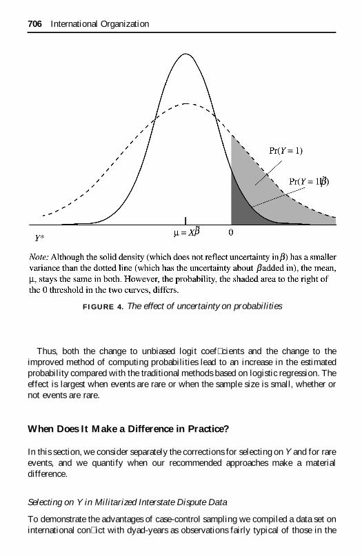
Thus, both the change to unbiased logit coef� cients and the change to theimproved method of computing probabilities lead to an increase in the estimatedprobability compared with the traditional methods based on logistic regression. Theeffect is largest when events are rare or when the sample size is small, whether ornot events are rare.

When Does It Make a Difference in Practice?

In this section, we consider separately the corrections for selecting on Y and for rareevents, and we quantify when our recommended approaches make a materialdifference.

Selecting on Y in Militarized Interstate Dispute Data

To demonstrate the advantages of case-control sampling we compiled a data set oninternational con� ict with dyad-years as observations fairly typical of those in the

FIGURE 4. The effect of uncertainty on probabilities


literature.24 The outcome variable is coded 1 if the dyad was engaged in a“militarized interstate dispute,” and 0 otherwise. The explanatory variables includethose typically used in this � eld, including whether the pair of countries includes amajor power, are contiguous, are allies, and have similar foreign policy portfolios.Also included are the balance of military power, the number of years since the lastdispute, and the nation in the dyad having the minimum and maximum degrees oftrade dependency and democracy.

Table 1 presents � ve analyses. The � rst column shows a traditional logisticregression on all 303,814 observations. The next column shows prior correctionapplied to data with 90 percent of the 0’s dropped, leaving only n 5 31,319observations. In the last column 99 percent of the 0’s have been dropped, resultingin only n 5 4,070 observations. For simplicity, and because of the large n, weignore the � nite sample and rare-events corrections for now.

The numerical results in the 90-percent column are fairly close to those in the fullsample, with standard errors that are only slightly higher. The analysis with 99percent of the 0’s dropped is also reasonably close to the full sample, but as expectedthe results are more variable. That the standard errors are slightly larger re� ects, andpredicts, this fact. Of the forty-four coef� cients in the four subsample columns, onlya few numbers vary enough to make much of a substantive difference in interpre-tation (such as indicating changes in signi� cance or magnitude). Of course, sincedeleting too many observations can decrease ef� ciency too much and make standarderrors unacceptably large, one must always consider the tradeoff between theef� ciency gained by including more observations and the resources saved by usingbetter variables. Collecting all dyads, as is now the universal practice, rarelyrepresents the optimal tradeoff, but the decision depends on the goals of theparticular application. Be aware that in interpreting Table 1, we expect somevariation across the rows due to random sampling. For example, if these columnswere analyses of independent random samples of the same size from the samepopulation, we would expect considerable variation across each row (with samplesof about 1,000, as is common, the 95-percent con� dence interval would be 66percent).

The explanatory variables chosen for this application re� ect approximately thestate of the art in this � eld but predict international con� ict only very weakly. Assuch, a key concern among researchers has been to � nd more meaningful andreliable measures, but the sheer magnitude of the data-collection task effectivelydictates far simpler, more arbitrary measures. Using a case-control design, aresearcher with a � xed budget can measure much more sophisticated explanatoryvariables. One way to think about the effort being saved or redirected would be toimagine collecting data for all 303,814 observations but having seventy-� ve timesas many researchers available to collect it (303,814/4,070). (This calculation

24. We began with all dyad-years from 1946 to 1992 available in Tucker 1998; merged variables fromBennett and Stam 1998a,b; and computed years since the last dispute using the program by Tucker 1999and using measures of alliance portfolios in Signorino and Ritter 1999.


exaggerates the savings for types of variables that are easier to measure in regionalor language clusters and for which an alternative method of selecting on Y might behelpful.) Variables that were previously infeasible to include using quantitativemethods but might now be worth collecting include trade commodity data (since theaggregate � gures do not distinguish between types of products and services),measures of leaders’ perceptions based on survey data or historical work, moremeaningful measures of physical proximity between countries than contiguity, andinformation on the process of strategic interaction as crises unfold.25 Collecting dataon each of these variables can be expensive; by reducing the number of observationsand thus the amount of data needed, we should be able to learn a great deal moreabout international con� ict than was previously possible.

25. Signorino 1999.

TABLE 1. Estimating the same parameters without 99 percent of the data

Explanatory variables Full sampleaPrior correction

(90% of 0’s dropped)bPrior correction

(99% of 0’s dropped)b

Contiguous 3.56 3.55 3.96(0.09) (0.10) (0.12)

Allies 20.27 20.21 20.28(0.09) (0.12) (0.15)

Foreign policy 0.23 0.45 0.38(0.20) (0.24) (0.26)

Balance of power 1.00 0.96 1.13(0.13) (0.15) (0.19)

Max. democracy 0.20 0.13 0.17(0.06) (0.07) (0.08)

Min. democracy 20.18 20.07 20.06(0.06) (0.07) (0.08)

Max. trade 0.05 0.05 0.05(0.01) (0.01) (0.01)

Min. trade 20.07 20.07 20.08(0.01) (0.01) (0.01)

Years since dispute 20.11 20.10 20.09(0.01) (0.01) (0.01)

Major power 1.31 1.81 2.2(0.09) (0.12) (0.14)

Constant 26.78 26.91 27.14(0.23) (0.26) (0.30)

n 303,814 31,319 4,070

Note: Numbers in parentheses are standard errors.aLogistic regression coef� cients based on a full sample.bLogistic regression coef� cients after prior corrections on data with 90 and 99 percent of Yi 5 0

observations randomly dropped.


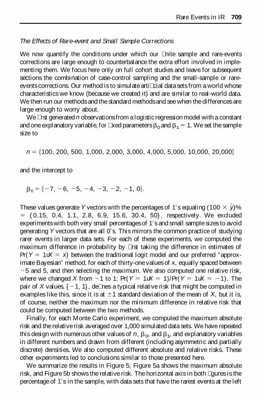
The Effects of Rare-event and Small Sample Corrections

We now quantify the conditions under which our � nite sample and rare-eventscorrections are large enough to counterbalance the extra effort involved in imple-menting them. We focus here only on full cohort studies and leave for subsequentsections the combination of case-control sampling and the small-sample or rare-events corrections. Our method is to simulate arti� cial data sets from a world whosecharacteristics we know (because we created it) and are similar to real-world data.We then run our methods and the standard methods and see when the differences arelarge enough to worry about.

We � rst generated n observations from a logistic regression model with a constantand one explanatory variable, for � xed parameters b0 and b1 5 1. We set the samplesize to

n 5 $100, 200, 500, 1,000, 2,000, 3,000, 4,000, 5,000, 10,000, 20,000%

and the intercept to

b0 5 $27, 26, 25, 24, 23, 22, 21, 0%.

These values generate Y vectors with the percentages of 1’s equaling (100 3 y# )%5 {0.15, 0.4, 1.1, 2.8, 6.9, 15.6, 30.4, 50}, respectively. We excludedexperiments with both very small percentages of 1’s and small sample sizes to avoidgenerating Y vectors that are all 0’s. This mirrors the common practice of studyingrarer events in larger data sets. For each of these experiments, we computed themaximum difference in probability by � rst taking the difference in estimates ofPr(Y 5 1 u X 5 x) between the traditional logit model and our preferred “approx-imate Bayesian” method, for each of thirty-one values of x, equally spaced between25 and 5, and then selecting the maximum. We also computed one relative risk,where we changed X from 21 to 1: Pr(Y 5 1 u X 5 1)/Pr(Y 5 1 u X 5 21). Thepair of X values, {21, 1}, de� nes a typical relative risk that might be computed inexamples like this, since it is at 61 standard deviation of the mean of X, but it is,of course, neither the maximum nor the minimum difference in relative risk thatcould be computed between the two methods.

Finally, for each Monte Carlo experiment, we computed the maximum absoluterisk and the relative risk averaged over 1,000 simulated data sets. We have repeatedthis design with numerous other values of n, b0, and b1, and explanatory variablesin different numbers and drawn from different (including asymmetric and partiallydiscrete) densities. We also computed different absolute and relative risks. Theseother experiments led to conclusions similar to those presented here.

We summarize the results in Figure 5; Figure 5a shows the maximum absoluterisk, and Figure 5b shows the relative risk. The horizontal axis in both � gures is thepercentage of 1’s in the sample, with data sets that have the rarest events at the left


of the � gure. For visual clarity, the horizontal axis is on the original logit scale;labeled percentages are (100 3 y# )%, but the tick marks appear at values of b0. InFigure 5a, the vertical axis is the maximum difference in absolute risk estimated bythe two methods; for visual clarity, it is presented on the log scale. In Figure 5b, thevertical axis is the absolute difference in relative risk, again on the log scale. Oneline is given for each sample size.

Several conclusions are apparent from Figure 5. First, as can be seen bycomparing the lines within either panel, the smaller the sample size, the higherthe line, and thus the greater the effect of our method. Second, since each lineslopes downward, the rarer the events in a data set, the larger the effect ofswitching methods. Clearly, sample size and rareness of events are exchangeablein some way since both measure the quantity of information in the data.

FIGURE 5. Logit-Bayesian differences in (a) absolute risk and (b) relative risk asa function of sample size and rareness of events


We now examine the speci� c numerical values. To understand these numbers,it is important to appreciate that what may seem like small values of theprobabilities can have overwhelming importance in substantive analyses ofgenuine rare-events data. For example, if a collection of 300,000 dyads showsa 0.001 increase in the probability of war, the � nding is catastrophicallyimportant because it represents about three hundred additional wars and amassive loss of human life. Relative risks are typically considered important inrare-event studies if they are at least 10 –20 percent, but, of course, they canrange much higher and have no upper limit. In Scott Bennett and Allan Stam’sextensive analysis of con� ict initiation and escalation in all dyads, for example,a majority of the sixty-three relative risks they report have absolute values ofless than 25 percent.26

By these comparisons, the numerical values on the vertical axis of Figure 5a aresizeable and of Figure 5b are very large. For a sample with 2.8 percent 1’s, thedifference in relative risk between the methods is about 128 percent for n 5 500.This means that when the logit model estimate of a treatment effect (that is, a givenchange in X) increases the risk of an event by 10 percent, for example, the estimatein our suggested method will increase the risk by 128 percent on average. This is avery substantial difference. Under the same circumstances, the difference betweenthe methods in relative risk is 63 percent for n 5 1,000, and 28 percent for n 52,000. For 1.1 percent 1’s, our preferred method differs from logit, on average, by332 percent for n 5 500, 173 percent for n 5 1,000, and 78 percent for n 52,000. These differences are well above many of the estimated relative risksreported in applied literatures.

For absolute risk, with 2.8 percent 1’s, the difference in the methods is about3 percent for n 5 500, 2 percent for n 5 1,000, and 1 percent for n 5 2,000. With1.1 percent 1’s, the difference between the logit and Bayesian methods in absoluterisk is about 4 percent for n 5 500, 3 percent for n 5 1,000, and 2 percent for n 52,000. These differences in absolute risk are larger than the reported effects formany rare-events studies. The main exceptions are for those studies able to predictrare events with high levels of accuracy (so that estimates of pi are large when Yi 51). Of course, Figure 5 reports the average differences in absolute and relative riskbetween logit and our preferred method; the real effect in any one application canbe larger or smaller.

Figure 5 also demonstrates that no sample size is large enough to evade � nitesample problems if the events are suf� ciently rare. For example, when n 5 20,000and 0.15 percent of the sample are 1’s, the difference between the existing methodsand our improved methods is 1.8 percent in absolute risk and 53.5 percent in relativerisk.

26. Bennett and Stam 1998b, tab. 4. We translated their reported relative risk to our percentage� gure—if r was their measure, ours is 100(r 2 1).


Rare-event Corrections in Deterrence Outcomes

We illustrate our methods here by reanalyzing Paul Huth’s analysis of the deter-minants of deterrence outcomes.27 We reproduced his probit analysis (from hisTable 1), reran the data with logit (which changed nothing important), and thenapplied our techniques. Huth’s analysis predicts the probability of deterring anaggressor as a function of the military balance of forces, the countries’ bargainingbehaviors, and their reputation earned in past deterrence episodes. The data include� fty-eight observations and about 58 percent 1’s. Although this is not a rare-eventssituation, recall that a small number of observations is equivalent, and according toFigure 5 Huth’s case should be approximately equivalent in terms of the effects ofour method to a data set with n 5 1,000 and 2.4 percent 1’s, or n 5 2,000 and 1.2percent 1’s.

For simplicity, we focus only on Huth’s � rst two substantive interpretations.28

Table 2 summarizes our reanalyses for the change in absolute risk (a � rst difference)and relative risk resulting from a change in the immediate balance of military forces,holding other variables constant at their means. For example, according to thetraditional logit approach, a change in the balance of forces from a 1:4 disadvantagefor the defender to equality increases the probability of deterrence success by 19.5percentage points. In contrast, our approximate Bayesian approach gives a muchsmaller effect of only 11.9 points. (Our approach reduces the effect, rather thanincreasing it, because y# . 0.5.) Using traditional logit methods to measure relativerisk yields an estimate of 40.1 percent, but our method suggests a more modesteffect of only 23.2 percent. Similar reductions also occur when changing the balanceof military forces from equality to 3:1 for the defender, as in the second row of Table2. Overall, our approach produces fairly large and substantively meaningfulchanges.

27. Huth 1988.28. Huth 1988, 437.

TABLE 2. Replication of “extended deterrence and the outbreak of war” fromHuth 1988

Change in balance of military forces First difference Relative risk

Logit Bayes Logit Bayes1:4 to 1:1 19.5% 11.9% 40.1% 23.2%1:1 to 3:1 26.9% 16.8% 39.6% 26.4%

Note: The “� rst difference” is the difference between two absolute risks as the balance of militaryforces changes (as indicated in the � rst column) (n 5 58).


Corrected Forecasts of State Failure

Finally, we include an analysis of data taken from the U.S. government’s StateFailure Task Force.29 We use all data for all European nations since the fall of theSoviet Union (n 5 348). State failure includes the collapse of the authority of thecentral government to impose law and order, such as occurs during civil war ordisruptive regime transitions. As in King and Zeng, the explanatory variables usedto explain state failure include the size of the military relative to the size of the totalpopulation, population density, legislative effectiveness, democracy (coded into twoindicator variables representing autocracy, and partial and full democracy), tradeopenness, and infant mortality.30 The fraction of state failures in the data is 1.15percent.

Our previous results, and those of the State Failure Task Force, indicate thatinfant mortality is a key indicator of state failure. The assumption is that keepinginfant mortality low tends to be an important goal of all governments. Countries thatare unable to meet this goal tend to be at greater risk of state failure, whether or notthey are democratic, have low military populations, have high trade openness, andso on. We computed the relative risk of state failure from the usual logit model bychanging infant mortality from 30 percent of the world median to the world median(or roughly one standard deviation below to one standard deviation above the infantmortality rate for cases with state failure in Europe since 1990). This change,holding other variables constant at their median, yields a relative risk of 33.4. Thus,according to the usual logit model, a nation with infant mortality at 30 percent of theworld median level of infant mortality has 33.5 times higher probability of statefailure than a nation at the world median. When corrected, our more accurate pointestimate of relative risk drops to only 10.2. This estimate has smaller mean squareerror and less bias. The 90-percent con� dence interval is wide but still lower thanthe standard logit point estimate, ranging from 5.0 to 29.1.

Concluding Remarks

We have discussed how to make the best use of existing rare-events data and howto improve data-collection efforts in the future. To improve existing rare-eventsdata, we offered the intuition behind easy-to-use methods for replacing logisticregression technology to reduce bias and increase accuracy with little cost. Toimprove future data-collection efforts, more essential from the perspective ofquantitative studies of international con� ict, we offered alternative strategies forcollecting data. These strategies will enable scholars to collect much more infor-mative data on a far smaller sample of cases without losing much informationneeded to make inferences to the entire population of nations or dyads globally.

29. Esty et al. 1998a,b.30. Ibid.


Analysts have spent considerable resources over the years amassing large andimpressive data collections regarding international con� ict, but qualitative research-ers still rightly complain that these collections miss much of the substance of theproblem, code only simplistic variables, and contain relatively little informationdespite their size. The methods we propose here enable researchers to code far bettervariables without increasing their costs. Perhaps this will help to narrow the rift inpolitical science between quantitative and qualitative approaches to explaininginternational con� ict.

When analysts use these alternative data-collection strategies, the populationfraction of events will still be rare, and the resulting samples will often be fairlysmall. The methods we propose allow researchers to correct estimates in alternativesampling designs and in rare-events data. The use of both types of corrections willbe synergistically more useful than either one alone.

References

Achen, Christopher A. 1999. Retrospective Sampling in International Relations. Paper presented at the57th Annual Meeting of the Midwest Political Science Association, Chicago.

Beck, Nathaniel, Gary King, and Langche Zeng. 2001. Improving Quantitative Studies of InternationalCon� ict: A Conjecture. American Political Science Review 94 (1):21–35.

Bennett, D. Scott, and Allan C. Stam, III. 1998a. EUGene: Expected Utility Generation and DataManagement Program. Version 1.12. Available at ^http://wizard.ucr.edu/cps/eugene/eugene.html?.

———. 1998b. Theories of Con� ict Initiation and Escalation: Comparative Testing, 1816–1980. Paperprepared for the annual meeting of the International Studies Association, Minneapolis.

Breslow, Norman E. 1996. Statistics in Epidemiology: The Case-control Study. Journal of the AmericanStatistical Association 91 (433):14–28.

Breslow, Norman E., and N. E. Day. 1980. Statistical Methods in Cancer Research. Lyon: InternationalAgency for Research on Cancer.

Bueno de Mesquita, Bruce. 1981. The War Trap. New Haven, Conn.: Yale University Press.Bueno de Mesquita, Bruce, and David Lalman. 1992. War and Reason: Domestic and International

Imperatives. New Haven, Conn.: Yale University Press.Cosslett, Stephen R. 1981. Ef� cient Estimation of Discrete-Choice Models. In Structural Analysis of

Discrete Data with Econometric Applications, edited by Charles F. Manski and Daniel McFadden,51–111. Cambridge, Mass.: MIT Press.

Esty, Daniel C., Jack Goldstone, Ted Robert Gurr, Barbara Harff, Marc Levy, Geoffrey D. Dabelko,Pamela T. Surko, and Alan N. Unger. 1998. The State Failure Task Force Report: Phase II Findings.McLean, Va.: Science Applications International Corporation.

Esty, Daniel C., Jack Goldstone, Ted Robert Gurr, Barbara Harff, Pamela T. Surko, Alan N. Unger, andRobert S. Chen. 1998. The State Failure Project: Early Warning Research for U.S. Foreign PolicyPlanning. In Preventive Measures: Building Risk Assessment and Crisis Early Warning Systems, editedby John L. Davies and Ted Robert Gurr, 27–38. Lanham, Md.: Rowman and Little� eld.

Geller, Daniel S., and J. David Singer. 1998. Nations at War: A Scienti� c Study of International Con�ict.New York: Cambridge University Press.

Holland, Paul W., and Donald B. Rubin. 1988. Causal Inference in Retrospective Studies. EvaluationReview 12 (3):203–31.

Huth, Paul K. 1988. Extended Deterrence and the Outbreak of War. American Political Science Review82 (2):423–43.


http://wizard.ucr.edu/cps/eugene/eugene.html?

Hsieh, David A., Charles F. Manski, and Daniel McFadden. 1985. Estimation of Response Probabilitiesfrom Augmented Retrospective Observations. Journal of the American Statistical Association 80(391):651–62.

Imbens, Guido. 1992. An Ef� cient Method of Moments Estimator for Discrete Choice Models withChoice-Based Sampling. Econometrica 60 (5):1187–1214.

King, Gary, and Langche Zeng. 2000. Estimating Risk and Rate Levels, Ratios, and Differences inCase-Control Data. Available at ^http://gking.harvard.edu&.

———. Forthcoming. Improving Forecasts of State Failure. World Politics.King, Gary, Robert O. Keohane, and Sidney Verba. 1994. Designing Social Inquiry: Scienti�c Inference

in Qualitative Research. Princeton, N.J.: Princeton University Press.King, Gary, Michael Tomz, and Jason Wittenberg. Forthcoming. Making the Most of Statistical

Analyses: Improving Interpretation and Presentation. American Journal of Political Science.Lancaster, Tony, and Guido Imbens. 1996a. Case-Control with Contaminated Controls. Journal of

Econometrics 71 (1–2):145–60.Levy, Jack S. 1989. The Causes of War: A Review of Theories and Evidence. In Behavior, Society, and

Nuclear War, vol. 1, edited by Phillip E. Tetlock, Jo L. Husbands, Robert Jervis, Paul C. Stern, andCharles Tilly, 2120–333. New York: Oxford University Press.

Manski, Charles F. 1999. Nonparametric Identi� cation Under Response-Based Sampling. In NonlinearStatistical Inference: Essays in Honor of Takeshi Amemiya, edited by C. Hsiao, K. Morimune, andJ. Powell. New York: Cambridge University Press.

Manski, Charles F., and Steven R. Lerman. 1977. The Estimation of Choice Probabilities fromChoice-based Samples. Econometrica 45 (8):1977–88.

Maoz, Zeev, and Bruce Russett. 1993. Normative and Structural Causes of Democratic Peace, 1946–86.American Political Science Review 87 (3):624–38.

Nagelkerke, Nico J. D., Stephen Moses, Francis A. Plummer, Robert C. Brunham, and David Fish. 1995.Logistic Regression in Case-control Studies: The Effect of Using Independent as Dependent Variables.Statistics in Medicine 14 (8):769–75.

Prentice, R. L., and R. Pyke. 1979. Logistic Disease Incidence Models and Case-control Studies.Biometrika 66 (3):403–11.

Ripley, Brian D. 1996. Pattern Recognition and Neural Networks. New York: Cambridge UniversityPress.

Rosenau, James N., ed. 1976. In Search of Global Patterns. New York: Free Press.Schaefer, Robert L. 1983. Bias Correction in Maximum Likelihood Logistic Regression. Statistics in

Medicine 2:71–78.Signorino, Curtis S. 1999. Strategic Interaction and the Statistical Analysis of International Con� ict.

American Political Science Review 93 (2):279–87.Signorino, Curtis S., and Jeffrey M. Ritter. 1999. Tau-b or Not Tau-b: Measuring the Similarity of

Foreign Policy Positions. International Studies Quarterly 43 (1):115–44.Tucker, Richard. 1998. The Interstate Dyad-Year Dataset, 1816–1997. Version 3.0. Available at

^http://www.fas.harvard.edu/;rtucker/data/dyadyear/&.———. 1999. BTSCS: A Binary Time-Series—Cross-Section Data Analysis Utility. Version 3.0.4.

Available at ^http://www.fas.harvard.edu/;rtucker/programs/btscs/btscs.html&.Vasquez, John A. 1993. The War Puzzle. New York: Cambridge University Press.


http://www.fas.harvard.edu/%7Ertucker/programs/btscs/btscs.html

http://www.fas.harvard.edu/%7Ertucker/data/dyadyear/


explaining rare events in international relations - gary king

Documents