experimental temperature/velocity control and implications

Experimental temperature/velocity control and implications for CFD

Presenters:• Koji Yasutomi, Hino Motors Ltd• Moez Ben Houidi, Pprime Institute, Poitiers, France• Russ Fitzgerald, Caterpillar

1

Participants: All ECN community!

Motivation

Do we know the initial conditions for Spray A?

What is the temperature distribution?

Is aerodynamics experimentally characterized?

How these parameters affect the spray results?

What kind of initial boundary conditions should we use for CFD?

2

3

Motivation: Simulation to experiment comparison

VP and LL comparison from Topic 3

• Small different behavior can be observed when comparing experiments from different ECN facilities

• Simulation is not always perfectly predictive

4

Motivation: Simulation to experiment comparisonID and LOL comparison from Topic 4/5

ECN 4 ECN 5

Under-prediction of shock tube data

result in a better match with

experimental results

Simulations use different chemistry and

turbulence models

Simulations are performed with a

uniform ambient temperature

hypothesis

What about initial turbulence kinetic

energy (not specified by experiments)?

How does uniform -T and velocity

assumptions affect simulation to

experiment comparison?

Injector protrudes into vessel 1.1 mm. Smallest cell size 0.125 mm.

Injector

Injector starts here

CONVERGE with homogenous-cell chemistryECN 3.0 Yuanjiang Pei and Sibendu Som

5

Motivation: Simulation with non-uniform T

% change 900 K

Liquid length 17.23

Ignition delay 16.0

Lift-off length 5.3

1100 K

27.5

6.0

8.1

Actual T delays ignition Asymmetric flame found in

simulation, but not systematically observed in experiments yet (SAE Paper, 2010-01-2106)

Retarded ignition will make the ignition delay pedictions even worse in topic 2!

Better chemical mechanism!!

ECN 3.0 Yuanjiang Pei and Sibendu Som

6

Motivation: Simulation with non-uniform T

At X = 2 mm, T decrease after injection which indicates that colder gas near the boundary layer is pulled in.

7

Motivation: Simulation with non-uniform TTemperature profiles in radial axis: effect of non-uniform T 1 ms after SOI


Position (X/Y = 0,6/0,3 mm)

7,6µm type K thermocouple

Temperature measurement during the injection (inert condition in the RCM of Pprime Institute)

MaxMin

Without injection With injection

Average

Injection aerodynamic bring colder gas into the spray (~43K lower)

Road Map

Initial boundary conditions can affect the spray characteristics

• Review temperature measurement in ECN facilities

• Collect boundary conditions (temperature and velocity) results from current ECN studies

• Try to understand their effects on spray and combustion

8

Discuss new recommendations for ECN spray A

[P.R.N. Childs, J.R. Greenwood and C.A. Long, Review of temperature measurement, Review of scientific instruments, volume71, Number 8, August 2000]

Noninvasive methods

Method Temperature

range

Min / Max(°C)

Response /

transient

capability

Accuracy Commercially

available / relative

cost

Rayleigh scattering 20 / 2500 Very fast / no 1% No / very high

Raman scattering 20 / 2227 Very fast / no 7% No / very high

CARS (Coherent Anti-

Stokes Raman

Scattering)

20 / 2000 Fast / NA 5% Yes / very high

LIF (Laser Induced

Fluorescence)

0 / 2700 Very fast / no 10% No / very high

Thermographic

phosphors

-250 / 2000 Very fast / yes 0,1%-5% Yes / highSemi-invasive

Optical methods can provide good spatial and temporal resolution however, they need prior development and a specific calibration for the quantitative measurement => expensive and difficult to install

CVP CPF/RCM/RCEM/Engines

Challenges • Minor species in post-preburn => may cause fluorescence quenching

• O2 quenching• Low quantum yield at high temperature levels• Calibration of the technique may be mandatory especially at such

high density and temperature levels

Review of temperature measurement techniques

9

Invasive method Temperature

range

Min / Max(°C)

Response /

transient

capability

Accuracy Commercially

available /

relative cost

Thermocouple -270 / 2300 Very fast / yes ±0.5-±2°C Yes / very low

Type G

Type K

Type R

• Thermocouples are cost-effective and accurate

temperature sensors

• Can be used in all ECN combustion facilities

• Thermocouples might have a catalytic effect in

oxidizing environment (type R for instance)

• Thermocouples might be altered by oxidation (this

can have a significant effect on emissivity)


10

+ long lifespan (minimized long term drift under cycling conditions)+ wires protected : can be used in corrosive environment with flowing materials (high robustness) - Slow response time

Sheathed thermocouples Bare-bead thermocouples

+ junction isolated from ground (avoid interference with instruments)+ faster response time- shorter lifespan- Inherently brittle

Ungrounded junction Grounded junction

junction protecteddifference in thermal expansion between the sheath and

junction materials may cause severe mechanical stress

junction isolated from ground Ground loops may cause interference with instruments

defects in insulation may be

easily detectedare more difficult to detect

slow response time faster response time


11

Sheath tip

Sheath / support

Thermocouple junction

Thermocouple wires

Insulation (often MgO)

The magnesium oxidehas a high dielectric strength, responds quickly to temperature changes, and is very durable

Why is response time too slow?

Measured temperature Tj depend on heat conduction from the sheath to the junction through the insulation and the thermocouple wires => thermal inertia does not only depend on the size of the junction but on the ensemble {sheath (s), insulation (i), junction(j) and wires (w) }

In such configuration, thermal conduction in the axial direction of the sheath has a significant impact on measured temperatureAssuming that heat transfer is purely in the axial direction under steady state conditions, the axial heat flow may be modeled: λ is thermal conductivity and A is cross sectional area

Such thermocouple are intended to measure temperature under steady state conditions

𝑄𝑥 = −෪𝜆𝐴𝑑𝑇

𝑑𝑥

෪𝜆𝐴 = 𝜆𝑤𝐴𝑤 + 𝜆𝑖𝐴𝑖 + 𝜆𝑠𝐴𝑠

Measurements are not resolved in space and time

Sheathed thermocouple with ungrounded junction


12

[Tagawa et al. Response compensation of fine-wire temperature sensors, review of scientific instruments 76, 094904, 2005]

Schematic of bare-bead ungrounded fine wire thermocouple

The frequency response of such thermocouple configuration is extensively modeled in literature (energy balance + temperature expressed as Fourier integrals)

Hypothesis:• Fine wires: temperature radially

homogeneous => conduction is considered in axial direction x (for instance when T prongs is lower than T wires)

• Heat transfer through: catalytic reactions on the junction, viscous dissipation and thermoelectric effects are neglected

Simulated frequency response of a 25µm type K thermocouple with various probe

configurations

Recommendations to minimize conduction

effects: L>>d2 and d2 = d1

Response compensation of fine wire thermocouples

13

[Paranthoën and Lecordier, Mesures de température dans les écoulements turbulents, Rev Gén Therm, (1996) 35, 283-308]

Cooled length, introduced by Betchov

and Corrsin

𝐿

𝑙𝑐> 10

𝐿

𝑑2≥ 400≈

𝑑1

𝑑2< 2.5

𝑑1

𝑑2

d1 and d2 as small as possible

Recommendations for the thermocouples design

14

TU/e, type Rdw = 50 µmdj = 100 µm

Prisme (Orleans, France), type Kdw = 13 µmdj = 39 µm

Pprime (Poitiers, France), type Kdw = 7.6 µmdj = ~ 8 to 14 µm

τ𝑠𝑒𝑒𝑛𝑠𝑜𝑟τ𝑤𝑖𝑟𝑒

𝜏 =𝜌𝑗𝐶𝑗𝑑𝑗

4ℎ𝑇𝑔 = 𝑇𝑗 + 𝜏

𝑑𝑇𝑗

𝑑𝑡+

𝜎𝜀

ℎ𝑇𝑗

4 − 𝑇𝑠4

Review of error correction / response compensation

Collis and Williams for 0.02 < Re < 44:

𝑁𝑢 = (0.24 + 0.51𝑅𝑒0.45)𝑇𝑓

𝑇𝑔

0.17

𝑇𝑓 =𝑇𝑗 + 𝑇𝑔

2

Cj = f(Tj) and ε=f(Tj)

h = f(Tf,ρf,V) ; thermal conductivity and dynamic viscosity of surrounding gas at film temperature Tf

Main issue is to find a good estimation of the cross flow velocity through the junction

ℎ =𝑁𝑢𝜆𝑔

𝑑

• Using a 12,7 µm wire instead of 7,6 µm double the correction (measured temperature increase rate ~17,6 K/ms)

• 1 m/s under-estimation of velocity => 6 K higher correction (example of a type K 12,7µm wire thermocouple, measured temperature increase rate ~17,8 K/ms)

• 1000 W/m².K under-estimation of h (heat coefficient) => 2 K higher correction (example of a type K 12,7µm wire thermocouple, measured temperature increase rate ~17,6 K/ms)


15

Spatial heterogeneities from available data

• Temperature heterogeneities are observed in all facilities• How to calculate the density ?

[Sandia data are presented by distribution of Tcore measured/Tcore_predicted]

Spatial heterogeneities

16

17

Spray A ID and LOL results

Prisme and Pprime: RCMSandia, IFPEN, TU/e: CVP

Temperature distribution is uniform on horizontal, except near the cold injector

At < 10 mm from injector, T decreasesBut lift-off length is only 16 mm

18

Temperature distribution from different facilities

Temperature drop at the thermal boundary is less effect at the GM and CAT case, but we doubt the accuracy of collection.

19

Temperature distribution from different facilities

Limitations of sheath TC measurements. Incorporate corrections.

20

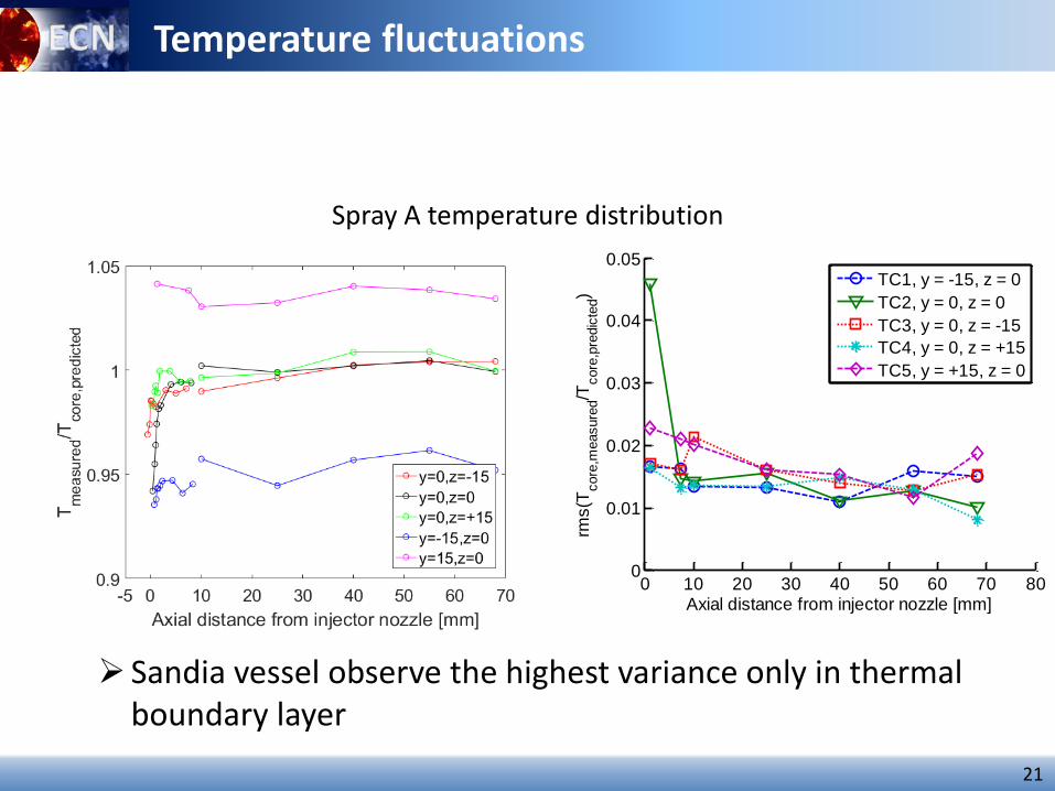
Temperature fluctuations

0 10 20 30 40 50 60 70 800

0.01

0.02

0.03

0.04

0.05

Axial distance from injector nozzle [mm]

rms(T

core

,measure

d/T

core

,pre

dic

ted)

TC1, y = -15, z = 0

TC2, y = 0, z = 0

TC3, y = 0, z = -15

TC4, y = 0, z = +15

TC5, y = +15, z = 0

Sandia vessel observe the highest variance only in thermal boundary layer

Spray A temperature distribution

21

The red is set at 0.8mm from laser entrance window—much lower than the measurements in the core, and much higher frequency. Suggests that if the injector were flush mounted, the temperature would be much less uniform.

Temperature distribution near the wall

Laser entrance window

22


Sandia injector protrudes 13mm from the flat wall

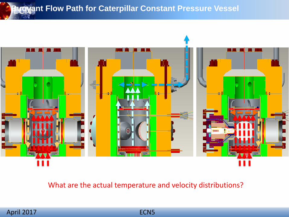
Buoyant Flow Path for Caterpillar Constant Pressure Vessel

What are the actual temperature and velocity distributions?

ECN5April 2017

Thermocouple Orientation for Temperature Characterization

Array of 24 thermocouples arranged to characterize vessel temperature:• K-type• 1mm sheath• Threaded through port

opposite injector holderMeasurements in multiple planes:• Three vertical planes at

varying axial distances• Vertical and horizontal

planes containing injector axis

ECN5April 2017

Temperature Distribution in Caterpillar Constant Pressure Vessel

ECN5April 2017

Objectives:

Measure mean velocity flowfields

Quantify spatially varying turbulent

fluctuations and length scales

Approach:

8Hz LaVision PIV system.

Seed flow with Superfine ZrO2 Powder

(500nm)

Density controlled by downstream

orifice and supply pressure

Timing optimized to minimize flow

disturbance and maximize signal

Acquire planar images at several

distances from injector tip location

200 shots / image pairs acquired for

flow field convergence.

Several magnifications and fields of

view used to verify turbulent

intensity and length scales.

Velocity Measurements in Caterpillar Constant Pressure Spray

Vessel

Test Conditions

PHTPV [bar] 60, 120

THTPV [K] 800, 900, 1000

Sheet Location

[mm]

10, 18, 24, 49, 75, 88

Lens [mm]

(magnification)

50, 105, 200

ECN5April 2017

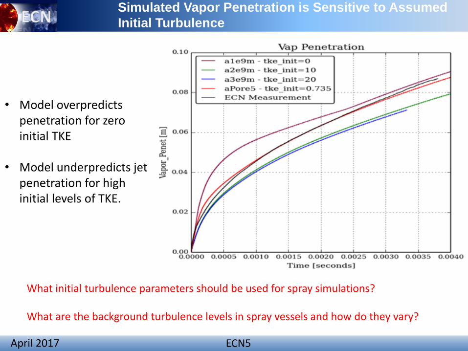
Simulated Vapor Penetration is Sensitive to Assumed

Initial Turbulence

What initial turbulence parameters should be used for spray simulations?

What are the background turbulence levels in spray vessels and how do they vary?

• Model overpredictspenetration for zero initial TKE

• Model underpredicts jet penetration for high initial levels of TKE.

ECN5April 2017

Modest effects of

ambient temperature

and pressure

Low bulk horizontal fluid

motion; local max

near center

Bulk vertical fluid motion

same order as in/out

flow; maximum near

cold injector holder

Isotropic turbulence near

vessel centerline

Vertical turbulent

component increases

quickly near injector

holder

Velocity Measurements Exhibit Consistent Trends Over Range of

ConditionsMean Velocities

Velocity Fluctuations

ECN5April 2017

Caterpillar

Constant

Pressure Vessel

Sandia Constant

Volume Vessel

(1000 rpm)

Mean Velocities: *0.12m/s

(.110/.055)

0.03m/s

(.028/.008)

Velocity

Fluctuations:

0.07m/s

(.065 / .077)

0.018m/s

(.017,.020)

Turbulent Kinetic

Energy:

0.008m2/s2 0.0005 m2/s2

Turbulent Length

Scale:

10-15mm unknown

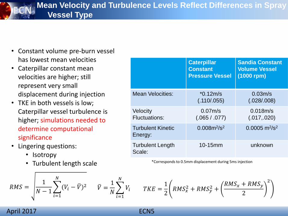
Mean Velocity and Turbulence Levels Reflect Differences in Spray

Vessel Type

• Constant volume pre-burn vessel has lowest mean velocities

• Caterpillar constant mean velocities are higher; still represent very small displacement during injection

• TKE in both vessels is low; Caterpillar vessel turbulence is higher; simulations needed to determine computational significance

• Lingering questions:• Isotropy• Turbulent length scale *Corresponds to 0.5mm displacement during 5ms injection

ECN5April 2017

𝑅𝑀𝑆 =1

𝑁 − 1

𝑖=1

𝑁

(𝑉𝑖 − ത𝑉)2 ത𝑉 =1

𝑁

𝑖=1

𝑁

𝑉𝑖 𝑇𝐾𝐸 =1

2𝑅𝑀𝑆𝑥

2 + 𝑅𝑀𝑆𝑦2 +

𝑅𝑀𝑆𝑥 + 𝑅𝑀𝑆𝑦

2

2

Velocity effect on temperature field?

Spray H conditions. 8000rpm 14.8kg/m3 Spray A conditions. 1000rpm 22.8kg/m3

Higher fan speed shows more uniform temperature fields

31

Velocity effect to the pre-burnMeijer et al., Atomization and Sprays 22(9):777-806 (2012)

IFPen Sandia TU/e

Fan speed (rpm) 3140 1000 1890

Lift-off length (mm) 15.4 16.5 15.8

Ignition delay (µs) 400 440 410

Faster cooldown DOES correspond to higher velocity and turbulence(Similar surface area to volume ratio in these chambers)

32

Velocity effect to the pre-burn

Fan speed affect to Initial turbulent kinetic energy.What is the effect of TKE to spray?

Spray A conditions (22.8 kg/m3)

33

Comparison of cool down Sandia (500,900,1200 rpm) , TUe (2000 rpm)

• Higher Fan speed => higher amplitude fluctuation at low frequencies

34

Velocity effect to the pre-burn in same facility

Ignition delay and LOL are described by temperature, not the “Fan speed”

Velocity effect to the Spray (Spray A fan speed sweep)

35

Velocity effect to the Soot (Spray A fan speed sweep)

Temperature field pocket -> Ignition delay and Lift-off length -> Soot

Spray characteristics do not change

36

Conclusion and Suggestions

Near the injector window, temperature drop is significant especially for constant volume chamber.

Constant pressure chamber showed slightly high TKE about 0.008 than constant volume vessel about 0.0005m/s

SUGGESTIONS for modeler Please use the non-uniform temperature distribution!!(We are not ready to propose the “one” temperature distribution which can explain the whole facility) To apply the TKE to simulation is also important to get “actual

temperature” fields.

37

Acknowledgements

Thanks Panos Sphicas (IC), Scott Skeen (Sandia), Scott Parrish (GM), Noud Maes (Tue), Michele Bardi (IFPEN), Ob Niphalai(Prisme), Tiexua (CMT) and Russ Fitzgerald (Caterpillar) for providing the temperature and velocity data of the vessel.

Thanks Lyle Pickett, Gilles Bruneaux and Raul Payri for encouraging for this topic session.

38

Backup Slides

Determination of Velocity Statistics

Vertical Plane: 24mm from Injector TipPa = 60bar, Ta = 900KΔt = 800µs, 50mm lens

Instantaneous Velocity𝑼 = ഥ𝑼 + 𝑼′

Mean Velocity𝑼

Velocity Fluctuations𝑼′

Spatially and Temporally Resolved Turbulence Statistics

Characteristics of HTPV Turbulence• Seeder adds some turbulence;

need to careful analyze data ‘after settling’

• Turbulence appears to be homogeneous and isotropic

• ‘Good vectors’ crucial for good turbulence statistics.

• Turbulence intensity is on the order of 25-30%

42


Tck7 Tc Tg7_NuTg7_Nu_m

in

Tg7_Nu_ma

x

effect of velocityVmeasur

ed0,05 1 m/s

930 936 936 939 934

9 4

Tck12 Tc Tg12_NuTg12_Nu_m

in

Tg12_Nu_ma

x

effect of velocityVmeasure

d2 3 m/s

830 873 869 872 866

42 36

dTj/dt = ~ 17k/ms

TU/e, type Rdw = 50 µmdj = 100 µmCorrection (SOI) = ~ 23 K

Prisme (Orleans, France), type Kdw = 13 µmdj = 39 µmCorrection (SOI) = ~ -21 to 28 K

Pprime (Poitiers, France), type Kdw = 7.6 µmdj = ~ 8 to 14 µmCorrection (SOI) = ~ -1 to 8 K

43

Review of temperature measurement in ECN facilities

Comparison of data from literature

Hypothesis Conduction convection Radiation total correction

Sandia SNL CVP Type-R : Pt/Pt+13Rh 50 µm Conduction error neglected no correction yes yes4 to 10 K (around 900

K)

TU/e CVP Type-R : Pt/Pt+13Rh 50 µm Conduction error neglected no correction yes yes4 to 10 K (around 900

K)

IFPEN CVP Type-K : Ni/Crsingle 50 µm or

25 µm?Conduction error neglected no correction yes yes

4 to 10 K (around 900

K)

Caterpillar CPF Type-K : Ni/Cr 1 and 3 mm

* Temperature is homogeneous in the small

volume where the different thermocouples

with different diameters are placed

* Temperature is averaged over 10 s

no correction

no correction

(temperature

averaged over time)

?

CMT CPF Type-K : Ni/Cr ?

* Temperature is homogeneous in the small

volume where the different thermocouples

with different diameters are placed

* Temperature is averaged over 20 s

no correction

no correction

(temperature

averaged over time)

?

PprimeRCM (single

shot)Type-K : Ni/Cr 7,6 µm Conduction error neglected no correction yes yes

2 to 4 K (around +-10

ms relative to SOI)

Error corrections Institution Facility Thermocouple type

Wires

dimension

𝑙 > 𝜏

𝜏 =𝜌 𝐶 𝑑

4ℎ

𝑇𝑔 = 𝑇𝑗 + 𝑑0 55

𝑇𝑔 = 𝑇𝑗 +𝜎𝜀 0 45𝑑0 55

0 5 0 45𝑇𝑗4 −𝑇𝑠

4 +𝑇𝑗

44

Sandia SNL CVP Type-R : Pt/Pt+13Rh 50 µm 461 K

* Std at 40 mm downstream of spray

axis: 11 K

* 45 K lower near the injector holder

* +-1% variation in spray axis

* +-4% variation in vertical axis +-15

mm

1- Meijer et al. Atomization and sprays, 22 (9)

2012

2- Pickett et al. SAE 2010-01-2106

TU/e CVP Type-R : Pt/Pt+13Rh 50 µm 443 K


axis: 12 K


2012


IFPEN CVP Type-K : Ni/Crsingle 50 µm or

25 µm?473 K


axis: 14 K

* +-2% variation in spray axis

* < +-4% variation in vertical axis +-15

mm


2012


Caterpillar CPF Type-K : Ni/Cr 1 and 3 mm 800 +- 5 K


(892 to 906 K within 3 mm from the

injector)


2012


CMT CPF Type-K : Ni/Cr ? 800 +-5 K

* Std in center volume downstream of

spray axis: 2,3 K (1 Hz logging)


(895 to 905 K within 3 mm from the

injector)


2012


PprimeRCM (single

shot)Type-K : Ni/Cr 7,6 µm 363 K


axis: 20 K

* spatial Std : 18 K

ECN France

Wires

dimensionWall temperature Heterogeneity level referenceInstitution Facility Thermocouple type

Review of temperature measurement in ECN facilities

Comparison of data from literature

45

Velocity data Pprime

Average velocity field(time average 20 ms)

Maximum velocity 0,7 m/s

Turbulence is estimated in the time window -10 to +10 ms after SOIIt is possible to recalculate TKE with smaller time range or with cyclic variations but at a lower density level

46

Pprime RCM vs CMT RCEM

experimental temperature/velocity control and implications

Documents