Loughborough UniversityInstitutional Repository

Experimental study of wavepropagation in

heterogeneous materials

This item was submitted to Loughborough University's Institutional Repositoryby the/an author.

Citation: DONA, M., LOMBARDO, M. and BARONE, G., 2015. Exper-imental study of wave propagation in heterogeneous materials. IN: Kruis, J.,Tsompanakis, J. and Topping, B.H.V. (eds.) Proceedings of the Fifteenth Inter-national Conference on Civil, Structural and Environmental Engineering Com-puting, Prague, 1-4 Sept, Paper 208.

Additional Information:

• This is a conference paper.

Metadata Record: https://dspace.lboro.ac.uk/2134/19245

Version: Accepted for publication

Publisher: c© Civil-Comp Limited

Rights: This work is made available according to the conditions of the Cre-ative Commons Attribution-NonCommercial-NoDerivatives 4.0 International(CC BY-NC-ND 4.0) licence. Full details of this licence are available at:https://creativecommons.org/licenses/by-nc-nd/4.0/

Please cite the published version.

Abstract

The phenomenon of wave propagation through concrete materials is affected by dis-persion due to its intrinsic heterogeneous microstructure. Previous experiments haveshown an increase of phase velocity at high frequencies. This behaviour cannot be ana-lytically described by the classical elasticity theory, due to its non-dispersive nature.Instead, enhanced theories can be adopted. In this work the dynamically consistentnon local model, able to take into account the microstructural effects by two addi-tional length scale parameters, is retrieved. The main subject of this contribution isthe experimental identification of the dispersive behaviour of cementitious materialsand the validation of the gradient continuum to predict the dispersion of the wave bornout of the heterogeneity of the material. The proposed work extends the applicabil-ity of non-local theories from a purely theoretical/analytical domain to the laboratoryterritory.

Keywords: Wave propagation, dispersion, gradient-enriched continuum.

1 Introduction

The propagation of elastic waves is largely used in many inspection techniques toestimate the quality and the integrity of a material. For example, concrete strengthand Young’s modulus are related through empirical relations to the pulse velocity,measured as the ratio between the travelled distance and the arrival time of the wave-form, identified as the first disturbance detected (BS EN 12504-4:2004 (2004); ASTMC215-14 (2014)). Further, knowledge of how stress waves propagate through a me-dium is important for non-destructive testing techniques based on ultrasonic testingand acoustic emissions.

Concrete is a composite material where coarse (3 to 30mm) and fine (0.1 to 3mm)

1

Experimental study of wave propagation in heterogeneous materials

M. Donà and M. Lombardo and G. Barone School of Civil and Building Engineering, Loughborough University, UK

15th The Fifteenth International Conference on Civil, Structural and Environmental Engineering Computing, CC 2015; Prague; Czech Republic; 1-4 September 2015

aggregates are joined together by a cement paste, resulting in a random heterogeneousmicrostructure (Aggelis and Polyzos (2004)). When elastic waves propagate throughsuch material, the internal inhomogeneities cause the generated signal to travel at dif-ferent velocities and to follow different travel paths before arriving to the receiver,exhibiting a dispersive behaviour, where waves of different frequencies travel at dif-ferent speeds. In particular, this behaviour is more noticeable when the wavelengthsare comparable or smaller than the size of the microstructure (the aggregate size inthis particular case).

The ultrasonic pulse velocity (UPV) technique is one of the most popular methodused for the assessment of structural integrity. For accurate characterisation of con-crete elements, since different variables affect the pulse velocity measurement, thewave characteristics should be considered to complement the wave velocity inform-ation. In fact, within the frequency range 10 - 300 kHz, the wave velocity increaseswith higher frequencies (Popovics et al. (1990); Aggelis et al. (2004)). This incrementis affected by several factors like moisture content, temperature, path length, shapeand size of the specimen, cracks and voids. (BS EN 12504-4:2004 (2004); Malhotraand Carino (2004)). The effect of aggregate size has been object of previous researchas for example in (Jacobs and Owino (2000); Molero et al. (2011)) who studied theattenuation of Rayleigh waves in concrete materials using laser ultrasonics and itsrelation to scattering phenomena and absorption, showing as the latter rules the at-tenuation mechanisms while the aggregate size does not affect it. Attenuation andpropagation of ultrasonic waves have been used to obtain information about the sizedistribution of the aggregate in concrete beams (Gaydecki et al. (1992)). It has beenfound that the amount and type of aggregate significantly increase the pulse velocityif compared with cement paste (Malhotra and Carino (2004); Popovics et al. (1990)).In order to specifically study the effects of the aggregate size on the wave propagationphenomena, a few researchers (Anugonda et al. (2001); Becker et al. (2003); Moleroet al. (2011)) tested specimens made of Portland cement, water and glass spheres of auniform diameter. Among other variables, it is worth mentioning that the pulse velo-city is also affected by water-cement (w/c) ratio; increasing w/c ratios correspond toreduced pulse velocities (Aggelis and Polyzos (2004); Aggelis et al. (2004)).

Reliable non-destructive testing therefore requires better interpretation of the ex-perimental observations and the benefit of analytical predictions is that they facilitatesincreased understanding of nascent phenomena. Since in many practical situations themicrostructural features significantly influence the global response, accurate model-ling of wave propagation in heterogeneous media requires that the microstructure isaccounted for. Discrepancies between experimental observations and theoretical pre-dictions based on classical theories show that the latter are not adequate to capturewave dispersion because they do not accommodate information about the microstruc-ture within the continuum model. Several other formulations have been proposed to fixthis issue; analysis methods based on discrete modelling and on enhanced continuumtheories are the most common technique. In the first case, the heterogeneities aremodelled as a lattice of masses linked together through an energy balance; Iliopouloset al. (2015), for example, used a lattice model where the aggregates are simulated

2

as masses linked together through elastic springs representing the concrete matrix.Instead, in the enhanced continuum approaches the medium is treated as homogen-eous equivalent to the heterogeneous one and the microstructure is taken into accountby additional internal variables (Carta and Brun (2012)). Mindlin (Mindlin (1964))has been one of the first to develop one of these models, followed by many others as(Chen and Fish (2001); Askes et al. (2007); Bennett et al. (2007a); Askes and Aifantis(2011)) where the classical continuum theory is enriched with higher order gradientsof the field variables accompanied by length scale parameters.

Many studies available in literature propose new analytical models based on en-riched theories but only limited research has been devoted to the experimental identi-fication of the additional characteristic length scale parameters from wave propagationmeasurements (Carta et al. (2012)); this paper represents a step forward in this direc-tion. It focuses on the dynamically consistent gradient elasticity model (Metrikineand Askes (2002)) where two additional terms related to stiffness and inertia contribu-tion are introduced. It has been chosen because in its simplicity guarantees physicalconsistency and numerical stability. If compared with other methods, it allows the rep-resentation of the monotonically increasing dispersive behaviour of concrete which isin good agreement with experimental evidence.

In the proposed work, elastic longitudinal waves have been applied on one end ofa concrete beam and recorded on the opposite one using piezoelectric transducers. Inorder to obtain measurements at several distances, the concrete beam has been cutinto shorter beams and the experiment repeated for each part. In particular, in thiscontribution, the dispersion behaviour of concrete is experimentally investigated andcompared with the analytical prediction with the aim to demonstrate the potential andlimitations of this type of gradient model, but also to introduce the work that will beaccomplished in future investigations.

This paper is structured in five sections. First, the dynamically consistent gradientelasticity model is reviewed and its properties briefly discussed. Then, the propagationof longitudinal waves in concrete material is discussed in relation to the gradient elasti-city model presented in the previous section. In Section 4 the experimental equipmentand the testing procedure are described. Section 5 reviews the different methods usedto obtain the group velocity and phase velocity. Finally the results of the tests ondifferent concrete sample and, in particular, the dispersion curves are presented.

2 Wave Dispersion Model

Aim of this section is to investigate the suitability of the so called dynamically con-sistent gradient elasticity theory to predict wave dispersion in concrete (Metrikine andAskes (2002)). The derivation of the dispersion curve for a one-dimensional problemwill be briefly recapped and comparison between analytical results and experimentalobservations will demonstrate that the elastic wave dispersion in concrete can be cap-tured with an appropriate selection of the microstructural lengths.

3

0 2 4 6 8 10 12 14 16 18 200.8

0.9

1

1.1

1.2

k h/2

c ph/

c e

{`m/L = 0.016}{`m/L = 0.018}{`m/L = 0.02}{`m/L = 0.022}{`m/L = 0.024}

Figure 1: Dispersion curves for wave propagation in an axial bar with dynamicallyconsistent gradient elasticity (`s/L = 0.02)

The differential equation of motion for the one-dimensional problem reads:

ρ u − ρ `2m u ′′ = Eu ′′ − E`2

s u ′′′′ , (1)

where u = u(x) is the axial displacement; ρ is the mass density; E is the Young’smodulus; `s and `m are the length scale parameters related with the higher-order stiff-ness and inertia, respectively. In Eq. (1) the superimposed dot denotes time derivative,while the inverted comma ′ denotes spatial derivative.

Assuming u as a general harmonic wave of the form u = A exp(i k(x − cpht)), thedispersion relation is obtained from Eq. (1) as follows:

− ρ k2c2ph − ρ `2

m k4c2ph = −Ek2 − E`2

s k4 , (2)

where A is the amplitude, k is the wave number and cph is the phase velocity. Eq. (2)can also be written in terms of the phase velocity and the wave number as:

c2ph

c2e

=1 + `2

s k2

1 + `2m k2 (3)

where the velocity of classical elasticity ce =√

E/ρ. Eq. (3) is the dispersion relationfor the dynamically consistent model; depending on the values given to the lengthscale parameters, it predicts different material behaviours. Fig. 1 shows different dis-persion curves for a beam of length L = 1m and square cross section (side h = 0.1m).The properties assigned to the material, Young’s modulus E = 30GPa and the dens-ity ρ = 2400kg/m2, are similar to concrete. Five combinations of {`s; `m} have beenconsidered: `s/L = {0.02}; `m/L = {0.016, 0.018, 0.02, 0.022, 0.024}. It can be ob-served that when the length scale parameter related with the micro-inertia `m is lowerthan `s, the phase velocity cph is larger than the phase velocity of the classical elasti-city ce, while the opposite is valid when `s < `m. It is worth mentioning here thatwhen `s = `m, the classical elasticity model with no dispersive behaviour is restored(continuous line in Fig. 1).

4

0 20 40 60 80 100 120 140 160 1803.8

4

4.2

4.4

4.6

4.8

k [1/m]

c ph

[km/s

]Experimental - w/c = 0.375Experimental - w/c = 0.40Experimental - w/c = 0.45Theor - {`s = 0.15m, `m = 0.12m}Theor - {`s = 0.10m, `m = 0.09m}Theor - {`s = 0.11m, `m = 0.1m}

Figure 2: Experimental dispersion curves for wave propagation in concrete for thesame aggregate-cement ratio (a/c = 3) and four different water-cement ratio (w/c)(Philippidis and Aggelis (2005)) and corresponding dispersion curve obtained withthe dynamically consistent model.

The dynamically consistent theory has been proposed to model wave dispersionin discrete lattice (Askes et al. (2007)) or one-dimensional laminate (Bennett et al.(2007b)) where higher wave numbers propagate slower than the lower wave numbers,that is when `s < `m. Instead, it has been experimentally proved that concrete exhibitsthe opposite behaviour. As it can be observed in Fig. 2, the experimental dispersionresults are in good agreement with the analytical curves obtained from the dynamicallyconsistent model when the microstiffness length scale `s is higher than the microinertiacontribution `m.

3 Materials and equipments

The aim of this section is to present the preliminary experimental investigation thathas been carried out in concrete samples in order to optimize the procedure of pulsevelocity measurements at different frequencies. The experiments involved two dif-ferent mixes, the first one made of sand while the second one of sand and aggregatewith average size of 12mm, both mixed together with Portland cement and water (wa-ter over cement ratio w/c of 0.4). The concrete beam samples have a square section,with side of 100mm, and length ranging from100mm to 1m. These values have beenchosen following the Standard (BS EN 12504-4:2004 (2004)) which suggests a min-imum length of 100mm to avoid local effects of the aggregate, and a minimum sizeof the specimen related to the wavelength of the transducer. In this case the minimumrecommended lateral dimension was 74mm for the 54kHz transducer. Considering thesignificant effect of the moisture content on the pulse velocity, the same curing con-ditions on the hydration of the cement has been adopted for the different specimens.Figure 3 shows the cross sections for the two investigated samples: Fig. 3a shows the

5

(a) Mortar (b) Max aggr. size= 12mm

Figure 3: Cross sections of the tested concrete beams

beam made of mortar only; Figs. 3b shows the beam’s section made of aggregate withmaximum size of 12mm. In the last case the amount of aggregate and the amount ofsand were 80% and 40% of the total volume, respectively.

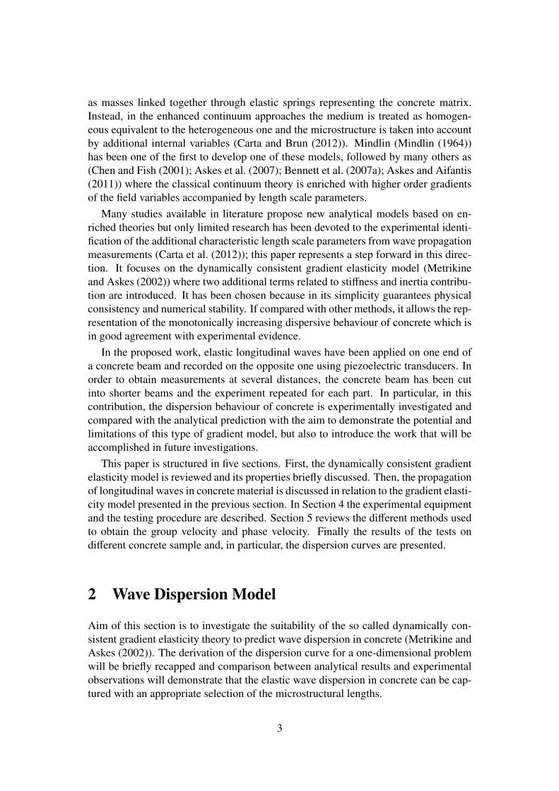
The experimental arrangement consists of two piezoelectric transducers coupled toboth end faces of the concrete beams using medium coupling grease (see Fig. 4). Oneof the transducer was excited to resonance by a Pundit pulser unit through a voltagepulse excitation while the second transducer was acting as receiver. The pulse appliedto excite the transducer had width on the range 1µs to 10µs and the voltage between125V to 500V. Even though the ultrasonic pulser is mainly used for field inspections,the repeatability of the generated waves allows to perform the experiment on differentbeams assuming that the same wave is applied each time. Similar experimental set-uphas been already used by several researchers for the laboratory experiments (Popovicset al. (1990); Long (2000)).

In order to study a range of frequencies where the material exhibits dispersive beha-viour, three pairs of narrow-band resonant transducers with different centre frequency(54kHz, 150kHz and 250kHz) have been used, covering then the lower end of theultrasonic range. For each sample, the test has been repeated several times, showinggood agreement on the measured shape and arrival time of the pulse wave.

3.1 The phase spectrum method - Fourier transform

Several techniques are available to evaluate the phase velocity from wave signals, asfor example the amplitude spectrum method, where the phase velocity is calculatedusing the longitudinal resonant frequencies combined with the mode numbers andthe distance between the boundaries of the specimen (Pialucha et al. (1989)); or theπ-point phase method which consists of determining the half-wavelength of an har-monic wave by varying the distance between transmitter and receiver transducers anddetermining the shift required to change the phase of the received signal by π; thephase velocity is then computed from continuous monochromatic waves or narrowband pulses (Papadakis (1976)). In this work the phase spectrum approach, as de-

6

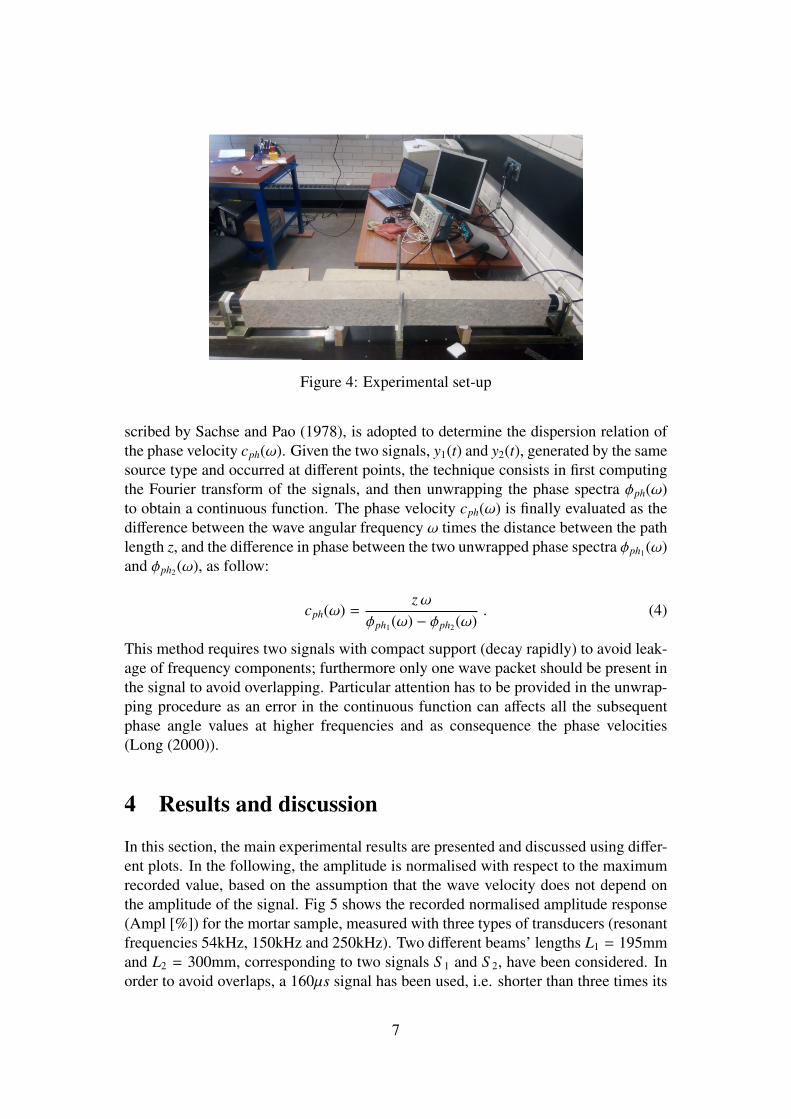
Figure 4: Experimental set-up

scribed by Sachse and Pao (1978), is adopted to determine the dispersion relation ofthe phase velocity cph(ω). Given the two signals, y1(t) and y2(t), generated by the samesource type and occurred at different points, the technique consists in first computingthe Fourier transform of the signals, and then unwrapping the phase spectra φph(ω)to obtain a continuous function. The phase velocity cph(ω) is finally evaluated as thedifference between the wave angular frequency ω times the distance between the pathlength z, and the difference in phase between the two unwrapped phase spectra φph1(ω)and φph2(ω), as follow:

cph(ω) =zω

φph1(ω) − φph2(ω). (4)

This method requires two signals with compact support (decay rapidly) to avoid leak-age of frequency components; furthermore only one wave packet should be present inthe signal to avoid overlapping. Particular attention has to be provided in the unwrap-ping procedure as an error in the continuous function can affects all the subsequentphase angle values at higher frequencies and as consequence the phase velocities(Long (2000)).

4 Results and discussion

In this section, the main experimental results are presented and discussed using differ-ent plots. In the following, the amplitude is normalised with respect to the maximumrecorded value, based on the assumption that the wave velocity does not depend onthe amplitude of the signal. Fig 5 shows the recorded normalised amplitude response(Ampl [%]) for the mortar sample, measured with three types of transducers (resonantfrequencies 54kHz, 150kHz and 250kHz). Two different beams’ lengths L1 = 195mmand L2 = 300mm, corresponding to two signals S 1 and S 2, have been considered. Inorder to avoid overlaps, a 160µs signal has been used, i.e. shorter than three times its

7

0 20 40 60 80 100 120 140 160−100 %

−50 %

0 %

50 %

100 %

t [µs]

Am

pl[%

]

Transducer 54kHzS 1 (195mm)S 2 (300mm)

0 20 40 60 80 100 120 140 160−100 %

−50 %

0 %

50 %

100 %

t [µs]

Am

pl[%

]

Transducer 150kHzS 1 (195mm)S 2 (300mm)

0 20 40 60 80 100 120 140 160−100 %

−50 %

0 %

50 %

100 %

t [µs]

Am

pl[%

]

Transducer 250kHzS 1 (195mm)S 2 (300mm)

Figure 5: Mortar sample – Normalised amplitude response (Ampl [%]) of two sig-nals S 1 and S 2 corresponding to two different lengths of the beam L1 = 195mm andL2 = 300mm, for three types of transducers (resonant frequency 54kHz, 150kHz and250kHz)

arrival time (55µs for L1 = 195mm).If we compare the shape of the received signal, for the same couple of transducers,

we can observe that they look similar. The dominant frequency of the signal is thesame as the resonant frequency of the transducer as we can clearly see in the amplitudespectra shown in Fig. 6 or Fig. 7 for the transducers with resonant frequencies of54kHz and 150kHz, respectively.

As suggested by Philippidis and Aggelis (2005), in order to obtain a consistentdispersion curve, the phase spectrum method was performed windowing the signalto reduced portions. Fig. 6 shows the amplitude spectrum (Ampl [%]) of signal S 1

recorded at the positions L1 = 195mm, with the transducer with resonant frequencyof 54kHz, as well as two portions of it, S 1, 2pks and S 1, 4pks, corresponding to the signaltruncated at the second and fourth peak, respectively. It can be observed that theoriginal signal S 1 has high amplitude in a clear frequency range around the resonance

8

0 20 40 60 80 100 120 140 160−100 %

−50 %

0 %

50 %

100 %

t [µs]

Am

pl[%

]Transducer 54kHzS 1

S 1, 2pks

S 1, 4pks

0 100 200 300 400

0 %

50 %

100 %

f [kHz]

|Am

pl|[%

]

Normalized Amplitude spectrum

S 1

S 1, 2pks

S 1, 4pks

Figure 6: Mortar sample – Normalised amplitude response (Ampl [%]) and amplitudespectrum (|Ampl|) of signal S 1 and two portions of it S 1, 2pks and S 1, 4pks recorded atthe positions L1 = 195mm, for the transducer with resonant frequency of 54kHz

0 20 40 60 80 100 120 140 160−100 %

−50 %

0 %

50 %

100 %

t [µs]

Am

pl[%

]

Transducer 150kHzS 1

S 1, 2pks

S 1, 4pks

0 100 200 300 400

0 %

50 %

100 %

f [kHz]

|Am

pl|[%

]

Normalized Amplitude spectrum

S 1

S 1, 2pks

S 1, 4pks

Figure 7: Mortar sample – Normalised amplitude response (Ampl [%]) and amplitudespectrum (|Ampl|) of signal S 1 and two portions of it S 1, 2pks and S 1, 4pks recorded atthe positions L1 = 195mm, for the transducer with resonant frequency of 150kHz

of the transducer, as well as the S 1, 4pks while for the signal S 1, 2pks , further relevantfrequencies appears. This suggests that the truncated signals have to be carefully usedin the phase spectrum method, where the phase of the signal plays a key role in thequantification of the phase velocity. Similarly, Fig. 7 shows the same for the transducerwith resonant frequency of 150kHz. Again, the less peaks we consider the smootheris the Fourier transform, but resulting to erroneously account for frequencies far fromthe resonance one.

The second example, shown in Fig. 8, is the signal recorded after propagatingthrough the concrete samples of two different lengths L1 = 600mm and L2 = 800mm,for the three types of transducers used in this work. In this case the time arrival for theshorter beam is about 150µs, so the duration of the signal was chosen to be 400µs. Itcan be observed that only for the 54kHz transducer the signals are smooth, while forthe remaining two it is more irregular, especially for the length of 800mm. This dis-

9

0 50 100 150 200 250 300 350 400−100 %

−50 %

0 %

50 %

100 %

t [µs]

Am

pl[%

]

Transducer 54kHzS 1 (600mm)S 2 (800mm)

0 50 100 150 200 250 300 350 400−100 %

−50 %

0 %

50 %

100 %

t [µs]

Am

pl[%

]

Transducer 150kHzS 1 (600mm)S 2 (800mm)

0 50 100 150 200 250 300 350 400−100 %

−50 %

0 %

50 %

100 %

t [µs]

Am

pl[%

]

Transducer 250kHzS 1 (600mm)S 2 (800mm)

Figure 8: Concrete sample – Normalised amplitude response (Ampl [%]) of twosignals S 1 and S 2 corresponding to two different positions L1 = 600mm and L2 =

800mm of the transducers, for three types of transducers (resonant frequency 54kHz,150kHz and 250kHz)

turbance can be explained as higher frequencies are strongly attenuated and the noiseover signal ratio increases for increasing length of the beam sample.

Signals truncated at the first peak S 1, 1pk and third peak S 1, 3pks have been represen-ted using the Fourier transform, for the concrete sample of L1 = 600mm and trans-ducer with resonant frequency of 54kHz (Fig. 9); while Fig. 10 shows the originalsignal S 1, the signal truncated at the second peak S 1, 2pk and the signal truncated at thefourth peak S 1, 4pk for the transducer with resonant frequency of 150kHz. As for themortar specimen, even though the portions of the signal have a smoother frequencyspectrum, they include different frequency content.

An attempt to evaluate the phase velocity starting from the frequency spectrumof the original signal and the truncated versions has been conducted using the phasespectrum method presented in section 3.1. The resulting dispersion curves for threedifferent portions of the signal are shown for the mortar in Fig. 11 and for the concrete

10

0 100 200 300 400−100 %

−50 %

0 %

50 %

100 %

t [µs]

Am

pl[%

]Transducer 54kHzS 1

S 1, 1pk

S 1, 3pks

0 100 200 300 400

0 %

50 %

100 %

f [kHz]

|Am

pl|[%

]

Normalized Amplitude spectrum

S 1

S 1, 1pk

S 1, 3pks

Figure 9: Concrete sample – Normalised amplitude response (Ampl [%]) and amp-litude spectrum (|Ampl|) of signal S 1 and two portions of it S 1, 1pk and S 1, 3pks recordedat the positions L1 = 600mm, for the transducer with resonant frequency of 54kHz

0 100 200 300 400−100 %

−50 %

0 %

50 %

100 %

t [µs]

Am

pl[%

]

Transducer 150kHzS 1

S 1, 2pks

S 1, 4pks

0 100 200 300 400

0 %

50 %

100 %

f [kHz]

|Am

pl|[%

]

Normalized Amplitude spectrum

S 1

S 1, 2pks

S 1, 4pks

Figure 10: Concrete sample – Normalised amplitude response (Ampl [%]) and amp-litude spectrum (|Ampl|) of signal S 1 and two portions of it S 1, 2pks and S 1, 4pks recordedat the positions L1 = 600mm, for the transducer with resonant frequency of 150kHz

sample in Fig. 12 and compared with the pulse velocity curve obtained with the Punditinstrument. In both cases, when the whole signal was used in the analysis, an irregu-lar dispersion curve was obtained. This behaviour can be explained as consequence ofthe limitation of the phase spectrum method in the unwrapping of an irregular phasespectrum. As expected from the frequency spectra in Figs. 6 -10, a smoother repres-entation is obtained when a truncated signal is used, especially with a truncation atthe second peak. Even though this last representation provides a slightly better ap-proximation of the expected dispersion curve, it was not taken into consideration forthe identification of the length scale parameters of the dynamically consistent modelbecause the windowed signals have been considered not representative of the materialbehaviour due to the different frequency content included. As consequence, the ana-lysis focused on the pulse velocity obtained with the pulser-receiver instrument andon the velocities of different peaks of the signal.

11

50 100 150 200 250 3000

2

4

6

8

10

f [kHz]

c ph

[km/s

]Mortar - whole signalMortar - 4pksMortar - 2pksMortar - Pulse Velocity

Figure 11: Experimental dispersion curves for wave propagation in mortar using thephase spectrum method.

50 100 150 200 250 3000

2

4

6

8

10

f [kHz]

c ph

[km/s

]

Concrete - whole signalConcrete - 4pksConcrete - 2pksConcrete - Pulse Velocity

Figure 12: Experimental dispersion curves for wave propagation in concrete using thephase spectrum method.

The pulse velocities for the mortar beam sample are summarised in Table 1, for thethree different transducers. In details, the table includes the pulse velocities measuredwith the Pundit instrument on L1 = 195mm, Vpundit,S 1; and L2 = 300mm, Vpundit,S 2; thepulse velocities of the first disturbance Vph,0 measured as the ratio between the lengthdifference L2 − L1 = 105mm and the time difference of the first recorded disturbanceof the signals S 1 and S 2; the velocity of the first peak V1stPk and second peak V2ndPk. Itcan be observed that in all the cases the pulse velocity slightly increases for increasingresonant frequency of the transducers, with an average increment of about +300m/s.Interestingly, the velocities of the first and second peaks are lower than those recordedby the Pundit, with V2ndPk being the lowest. Analogously, the pulse velocities for theconcrete beam sample are summarised in Table 2.

The dispersion curves for the pulse velocities measured using the Pundit instrumenton mortar and concrete are compared in Fig. 13. As expected, the velocity for concrete

12

f Vpundit,S 1 Vpundit,S 2 Vpulse,0 V1stPk V2ndPk

kHz [m/s] [m/s] [m/s] [m/s] [m/s]54kHz 3488 3513 3281 3387 3088

150kHz 3686 3597 3500 3387 3387250kHz 3721 3619 3620 3500 3387

Table 1: Five different evaluation of the pulse velocity [m/s] for the mortar beamsample: pulse velocity measured with the Pundit on L1, Vpundit,S 1; pulse velocity meas-ured with the Pundit on L2, Vpundit,S 2; pulse velocity first disturbance Vph,0; pulse velo-city first peak V1stPk; pulse velocity second peak V2ndPk

f Vpundit,S 1 Vpundit,S 2 Vpulse,0 V1stPk V2ndPk

kHz [m/s] [m/s] [m/s] [m/s] [m/s]54kHz 4228 4191 3975 4016 3997

150kHz 4367 4303 4280 4089 4115250kHz 4381 4458 4461 4449 4378

Table 2: Five different evaluation of the pulse velocity [m/s] for the concrete beamsample: pulse velocity measured with the Pundit on L1, Vpundit,S 1; pulse velocity meas-ured with the Pundit on L2, Vpundit,S 2; pulse velocity first disturbance Vph,0; pulse velo-city first peak V1stPk; pulse velocity second peak V2ndPk

is higher than the one in mortar, in particular the gap is about 1000m/s. This differenceis mainly due to the higher stiffness of the concrete if compared with the stiffness ofthe mortar.

5 Conclusions

In the present paper, the experimental ultrasonic wave propagation measurements onconcrete and mortar are presented. Narrow band waves of three different frequencies(54kHz, 150kHz and 250kHz) corresponding to the resonance of the transducers areintroduced into the mortar and concrete samples. The pulse velocity provided by thepulse generator has been compared with the velocity of different peaks of the sig-nal. An attempt to evaluate the phase velocity using the phase spectrum method wasconducted. The results highlighted how the data obtained using the resonance trans-ducers are not enough accurate to represent the dispersion behaviour in the wholerelevant range of frequencies (0kHz - 500kHz). The signals recorded with the reson-ant transducers were not able to provide reliable information outside of their reson-ance frequency. Considering only the three points available in the dispersion curve

13

54 150 2503

3.5

4

4.5

5

f [kHz]

v pul

se[k

m/s

]

ConcreteMortar

Figure 13: Dispersion curve for the pulse velocity of the beam made out of mortar andthe concrete beam with maximum aggregate size of 12mm.

for the pulse velocity, an accurate identification of the length scale parameters of thedynamically consistent model was not possible. In order to do that, more accurate ex-periments using broadband transducers connected to a wave generator, which allowsto investigate, for each frequency, the corresponding wave velocity for a more accuraterepresentation of the dispersion curve, are suggested for these analysis. The proced-ure can then be repeated for different concrete samples made using a specific rangeof aggregate size and the same cement-aggregate ratio and water-cement ratio. Oncethese curves will be available, they will be used to identify the length scale parametersand their variation with the different aggregate sizes.

6 Acknowledgements

EPSRC (UK) is gratefully acknowledged for funding this research project under grantEP/M004163/1.

References1. BS EN 12504-4:2004, . Testing concrete. determination of ultrasonic pulse velocity.

2004.

2. ASTM C215-14, . Standard test method for fundamental transverse, longitudinal, andtorsional frequencies of concrete specimens. 2014.

3. Aggelis, D., Polyzos, D.. Wave dispersion phenomena in concrete. In: Advances inScattering and Biomedical Engineering. World Scientific; 2004, p. 159–165.

4. Popovics, S., Rose, J.L., Popovics, J.. The behaviour of ultrasonic pulses in concrete.Cement and Concrete Research 1990;20(2):259–270.

14

5. Aggelis, D., Philippidis, T., Tsinopoulos, S., Polyzos, D.. Wave dispersion in con-crete due to microstructure. In: CD-ROM Proceedings of the 2004 Int. Conferenceon Computational & Experimental Engineering & Sciences. 2004, .

6. Malhotra, V.M., Carino, N.J.. Handbook on nondestructive testing of concrete. CRCpress; 2004.

7. Jacobs, L.J., Owino, J.O.. Effect of aggregate size on attenuation of rayleigh sur-face waves in cement-based materials. Journal of engineering mechanics 2000;126(11):1124–1130.

8. Molero, M., Segura, I., Aparicio, S., Fuente, J.V.. Influence of aggregates and airvoids on the ultrasonic velocity and attenuation in cementitious materials. EuropeanJournal of Environmental and Civil Engineering 2011;15(4):501–517.

9. Gaydecki, P., Burdekin, F., Damaj, W., John, D.. The propagation and attenuationof medium-frequency ultrasonic waves in concrete: a signal analytical approach.Measurement Science and Technology 1992;3(1):126.

10. Anugonda, P., Wiehn, J.S., Turner, J.A.. Diffusion of ultrasound in concrete. Ultra-sonics 2001;39(6):429–435.

11. Becker, J., Jacobs, L.J., Qu, J.. Characterization of cement-based materials usingdiffuse ultrasound. Journal of engineering mechanics 2003;129(12):1478–1484.

12. Iliopoulos, S.N., Polyzos, D., Aggelis, D.G.. New non-local lattice models forthe description of wave dispersion in concrete. In: SPIE Smart Structures andMaterials+ Nondestructive Evaluation and Health Monitoring; vol. 9436. 2015, p.94360C–94360C–10.

13. Carta, G., Brun, M.. A dispersive homogenization model based on lattice approxim-ation for the prediction of wave motion in laminates. Journal of Applied Mechanics2012;79(2):021019.

14. Mindlin, R.. Micro-structure in linear elasticity. Archive for Rational Mechanics andAnalysis 1964;16(1):51–78.

15. Chen, W., Fish, J.. A dispersive model for wave propagation in periodic hetero-geneous media based on homogenization with multiple spatial and temporal scales.Transactions-american society of mechanical engineers journal of applied mechan-ics 2001;68(2):153–161.

16. Askes, H., Bennett, T., Aifantis, E.. A new formulation and C0-implementationof dynamically consistent gradient elasticity. International Journal for NumericalMethods in Engineering 2007;72(1):111–126.

17. Bennett, T., Gitman, I., Askes, H.. Elasticity theories with higher-order gradients ofinertia and stiffness for the modelling of wave dispersion in laminates. InternationalJournal of Fracture 2007a;148(2):185–193.

15

18. Askes, H., Aifantis, E.C.. Gradient elasticity in statics and dynamics: an overview offormulations, length scale identification procedures, finite element implementationsand new results. International Journal of Solids and Structures 2011;48(13):1962–1990.

19. Carta, G., Bennett, T., Askes, H.. Determination of dynamic gradient elasticitylength scales. Proceedings of the ICE-Engineering and Computational Mechanics2012;165(1):41–47.

20. Metrikine, A., Askes, H.. One-dimensional dynamically consistent gradient elasti-city models derived from a discrete microstructure. part 1: Generic formulation.European Journal of Mechanics-A/Solids 2002;21(4):555–572.

21. Bennett, T., Gitman, I., Askes, H.. Elasticity theories with higher-order gradients ofinertia and stiffness for the modelling of wave dispersion in laminates. InternationalJournal of Fracture 2007b;148(2):185–193.

22. Philippidis, T., Aggelis, D.G.. Experimental study of wave dispersion and attenuationin concrete. Ultrasonics 2005;43(7):584–595.

23. Long, R.. Improvement of ultrasonic apparatus for the routine inspection of concrete.Ph.D. thesis; University of London; 2000.

24. Pialucha, T., Guyott, C., Cawley, P.. Amplitude spectrum method for the measure-ment of phase velocity. Ultrasonics 1989;27(5):270–279.

25. Papadakis, E.P.. Ultrasonic velocity and attenuation: Measurement methods withscientific and industrial applications. Physical acoustics 1976;12:277–374.

26. Sachse, W., Pao, Y.H.. On the determination of phase and group velocities of dis-persive waves in solids. Journal of Applied Physics 1978;49(8):4320–4327.

16