experimental method development for direct dosimetry of
TRANSCRIPT

Louisiana State UniversityLSU Digital Commons
LSU Master's Theses Graduate School
2005
Experimental method development for directdosimetry of permanent interstitial prostatebrachytherapy implantsJohn Michael JarrettLouisiana State University and Agricultural and Mechanical College, [email protected]
Follow this and additional works at: https://digitalcommons.lsu.edu/gradschool_theses
Part of the Physical Sciences and Mathematics Commons
This Thesis is brought to you for free and open access by the Graduate School at LSU Digital Commons. It has been accepted for inclusion in LSUMaster's Theses by an authorized graduate school editor of LSU Digital Commons. For more information, please contact [email protected].
Recommended CitationJarrett, John Michael, "Experimental method development for direct dosimetry of permanent interstitial prostate brachytherapyimplants" (2005). LSU Master's Theses. 2124.https://digitalcommons.lsu.edu/gradschool_theses/2124

EXPERIMENTAL METHOD DEVELOPMENT
FOR DIRECT DOSIMETRY OF PERMANENT INTERSTITIAL PROSTATE BRACHYTHERAPY IMPLANTS
A Thesis
Submitted to the Graduate Faculty of the Louisiana State University and
Agricultural and Mechanical College in partial fulfillment of the
requirements for the degree of Master of Science
in
The Department of Physics & Astronomy
By John Michael Jarrett
B.S., Southeastern Louisiana University, 1992 May 2005

TABLE OF CONTENTS
LIST OF TABLES.......................................................................................................... iv
LIST OF FIGURES ........................................................................................................ vi
ABSTRACT......................................................................................................................x
CHAPTER 1. PROSTATE BRACHYTHERAPY..........................................................1 1.1 Introduction...........................................................................................................1 1.2 Thesis Overview ...................................................................................................2 1.3 Prostate Cancer .....................................................................................................4 1.4 Clinical Rationale for Postimplant Dosimetry......................................................5 1.5 Postimplant Dosimetry Uncertainty......................................................................8 1.6 Seed Position and Orientation Factors................................................................10 1.7 Postimplant Edema .............................................................................................14 1.8 Physical Seed Characteristics Affecting Dosimetry ...........................................16 1.9 Tissue Heterogeneity ..........................................................................................18 1.10 Conclusion ..........................................................................................................18
CHAPTER 2. PET/CT IMAGING .................................................................................20 2.1 Introduction.........................................................................................................20 2.2 PET General Principles.......................................................................................21 2.3 2D Acquisition Versus 3D Acquisition ..............................................................22 2.4 Attenuation Correction........................................................................................23 2.5 Discovery ST PET/CT Scanner ..........................................................................25 2.6 Simulated Brachytherapy Seed Preparation........................................................26 2.7 Characteristics of the F-18 Positron Source........................................................27 2.8 Acrylic Prostate Phantom ...................................................................................29 2.9 Experimental Measurements...............................................................................30 2.10 Scan Set One—Six Acquisitions ........................................................................32 2.11 Scan Set Two—Four Acquisitions......................................................................34 2.12 Extracting Annihilation Event Density From PET DICOM Files ......................36 2.13 Data Reduction for MCNP Input—Pixel Data Significance ..............................36
CHAPTER 3. MCNP5 COMPUTATIONAL EXPERIMENTS....................................39 3.1 Introduction.........................................................................................................39 3.2 Simulation of Seed Geometry Dose Deposition .................................................40 3.3 Annihilation Source Geometry in the MCNP Simulation ..................................43 3.4 MCNP5 Energy Deposition Calculation Experiments .......................................45 3.5 MCNP5 Uncertainty Analysis ............................................................................45 CHAPTER 4. RESULTS AND CONCLUSIONS .........................................................46 4.1 Introduction.........................................................................................................46 4.2 Results.................................................................................................................46 4.3 Discussion...........................................................................................................54
ii

4.4 Conclusions.........................................................................................................58 REFERENCES ...............................................................................................................60 APPENDIX A. LIST OF MCNP5 COMPUTATIONAL EXPERIMENTS.................66 A.1 Energy Deposition Distributions Due to Theoretical Ideal Seed Sources ..........66 A.2 Energy Deposition Distributions Due to Voxel and Point Sources ....................67 A.3 Energy Deposition Distributions From Second Scan Measured Data ................71
APPENDIX B. GRAPHS AND TABLES OF COMPUTATIONAL RESULTS.........76
APPENDIX C. IDL DATA EXTRACTION PROGRAM FOR DICOM...................102
APPENDIX D. MCNP5 TUTORIAL...........................................................................103
APPENDIX E. DICOM STANDARD .........................................................................110
APPENDIX F. MCNP5 SAMPLE INPUT FILES.......................................................112 F.1 Theoretical Distribution....................................................................................112 F.2 Measured Distribution ......................................................................................114 VITA.............................................................................................................................120
iii

LIST OF TABLES
1. Three seed arrangement composition and seed locations used for scans ...................32
2. Acquisition parameters for Scan Set One ...................................................................32
3. Acquisition parameters for Scan Set Two ..................................................................35
4. Mass interaction coefficients listed for Water, Acrylic, and Tissue (ICRU 33 four component definition) for 500 keV photons.......................................................41
5. Material composition and mass density for materials used in MCNP input (courtesy
of Bristol-Myers Squibb Medical Imaging)........................................................42 6. Point versus volume source study cases .....................................................................53
7. Values plotted in Figure 9 and Figure 18 with associated MCNP error and relative discrepancy .........................................................................................................90
8. Values plotted in Figure 12 and Figure 19 with associated MCNP error and relative
discrepancy .........................................................................................................91 9. Values plotted in Figure 10 and Figure 20 with associated MCNP error and relative
discrepancy .........................................................................................................92 10. Values plotted in Figure 21 and Figure 22 with associated MCNP error and
relative discrepancy ............................................................................................93 11. Values plotted in Figure 11 and Figure 23 with associated MCNP error and
relative discrepancy ............................................................................................94 12. Values plotted in Figure 24 and Figure 25 with associated MCNP error and
relative discrepancy ............................................................................................95 13. Values plotted in Figure 26 and Figure 28 with associated MCNP error and
relative discrepancy ............................................................................................96 14. Values plotted in Figure 27 and Figure 29 with associated MCNP error and
relative discrepancy ............................................................................................97 15. Values plotted in Figure 30 and Figure 32 with associated MCNP error and
relative discrepancy ............................................................................................98 16. Values plotted in Figure 31 and Figure 33 with associated MCNP error and
relative discrepancy ............................................................................................99
iv

17. Values plotted in Figure 14 with associated MCNP error and actual and absolute error bounds ......................................................................................................100
18. Values plotted in Figure 34 with associated MCNP error and actual and absolute
error bounds ......................................................................................................100 19. Values plotted in Figure 13 and Figure 35 with associated MCNP error and
relative discrepancy ..........................................................................................101
v
LIST OF FIGURES
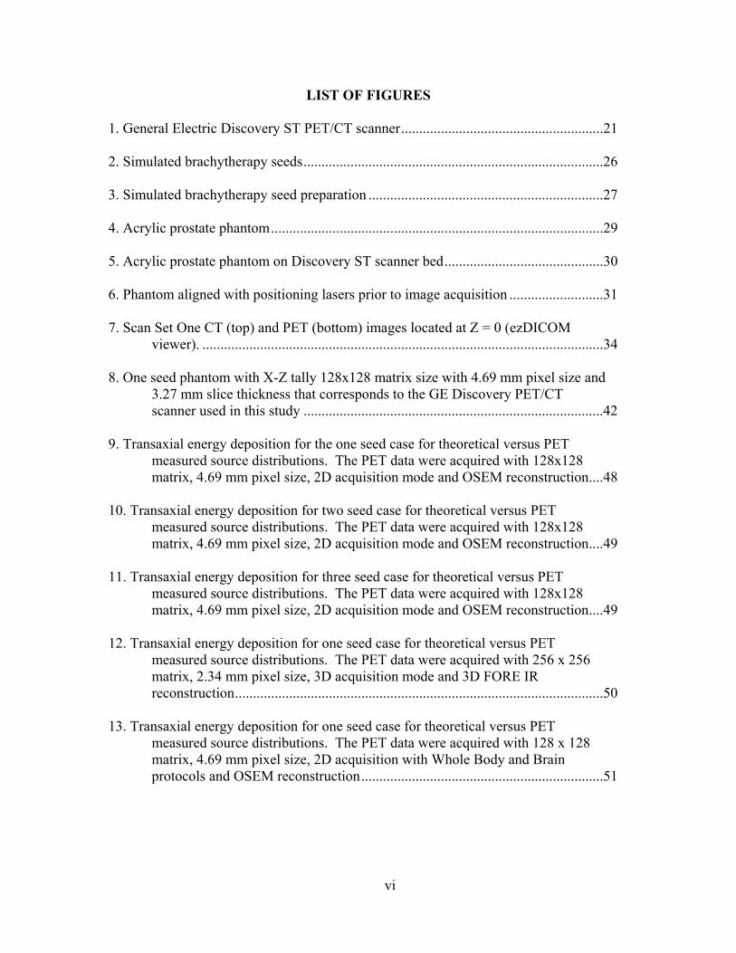
1. General Electric Discovery ST PET/CT scanner........................................................21
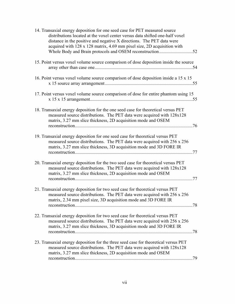
2. Simulated brachytherapy seeds...................................................................................26
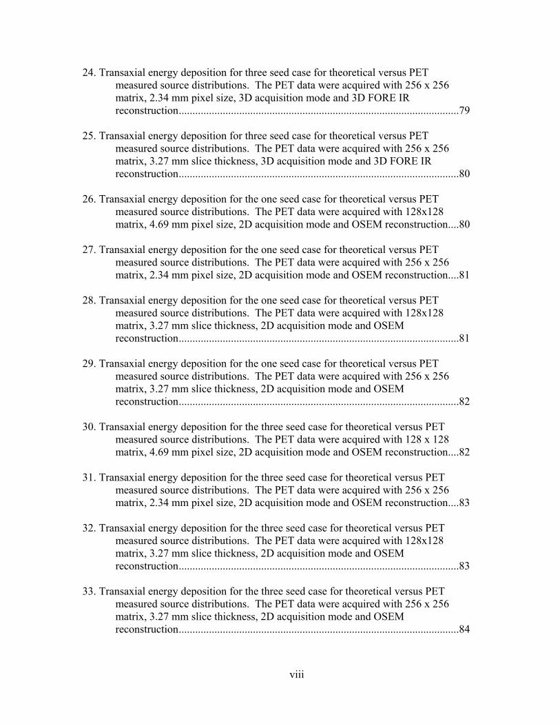
3. Simulated brachytherapy seed preparation .................................................................27
4. Acrylic prostate phantom............................................................................................29
5. Acrylic prostate phantom on Discovery ST scanner bed............................................30
6. Phantom aligned with positioning lasers prior to image acquisition ..........................31 7. Scan Set One CT (top) and PET (bottom) images located at Z = 0 (ezDICOM
viewer). ...............................................................................................................34 8. One seed phantom with X-Z tally 128x128 matrix size with 4.69 mm pixel size and
3.27 mm slice thickness that corresponds to the GE Discovery PET/CT scanner used in this study ...................................................................................42
9. Transaxial energy deposition for the one seed case for theoretical versus PET
measured source distributions. The PET data were acquired with 128x128 matrix, 4.69 mm pixel size, 2D acquisition mode and OSEM reconstruction....48
10. Transaxial energy deposition for two seed case for theoretical versus PET
measured source distributions. The PET data were acquired with 128x128 matrix, 4.69 mm pixel size, 2D acquisition mode and OSEM reconstruction....49
11. Transaxial energy deposition for three seed case for theoretical versus PET
measured source distributions. The PET data were acquired with 128x128 matrix, 4.69 mm pixel size, 2D acquisition mode and OSEM reconstruction....49
12. Transaxial energy deposition for one seed case for theoretical versus PET
measured source distributions. The PET data were acquired with 256 x 256 matrix, 2.34 mm pixel size, 3D acquisition mode and 3D FORE IR reconstruction......................................................................................................50
13. Transaxial energy deposition for one seed case for theoretical versus PET
measured source distributions. The PET data were acquired with 128 x 128 matrix, 4.69 mm pixel size, 2D acquisition with Whole Body and Brain protocols and OSEM reconstruction...................................................................51
vi
14. Transaxial energy deposition for one seed case for PET measured source distributions located at the voxel center versus data shifted one-half voxel distance in the positive and negative X directions. The PET data were acquired with 128 x 128 matrix, 4.69 mm pixel size, 2D acquisition with Whole Body and Brain protocols and OSEM reconstruction.............................52
15. Point versus voxel volume source comparison of dose deposition inside the source
array other than case one.....................................................................................54 16. Point versus voxel volume source comparison of dose deposition inside a 15 x 15
x 15 source array arrangement ............................................................................55 17. Point versus voxel volume source comparison of dose for entire phantom using 15
x 15 x 15 arrangement.........................................................................................55 18. Transaxial energy deposition for the one seed case for theoretical versus PET
measured source distributions. The PET data were acquired with 128x128 matrix, 3.27 mm slice thickness, 2D acquisition mode and OSEM reconstruction......................................................................................................76
19. Transaxial energy deposition for one seed case for theoretical versus PET
measured source distributions. The PET data were acquired with 256 x 256 matrix, 3.27 mm slice thickness, 3D acquisition mode and 3D FORE IR reconstruction......................................................................................................77
20. Transaxial energy deposition for the two seed case for theoretical versus PET
measured source distributions. The PET data were acquired with 128x128 matrix, 3.27 mm slice thickness, 2D acquisition mode and OSEM reconstruction......................................................................................................77
21. Transaxial energy deposition for two seed case for theoretical versus PET
measured source distributions. The PET data were acquired with 256 x 256 matrix, 2.34 mm pixel size, 3D acquisition mode and 3D FORE IR reconstruction......................................................................................................78
22. Transaxial energy deposition for two seed case for theoretical versus PET
measured source distributions. The PET data were acquired with 256 x 256 matrix, 3.27 mm slice thickness, 3D acquisition mode and 3D FORE IR reconstruction......................................................................................................78
23. Transaxial energy deposition for the three seed case for theoretical versus PET
measured source distributions. The PET data were acquired with 128x128 matrix, 3.27 mm slice thickness, 2D acquisition mode and OSEM reconstruction......................................................................................................79
vii
24. Transaxial energy deposition for three seed case for theoretical versus PET measured source distributions. The PET data were acquired with 256 x 256 matrix, 2.34 mm pixel size, 3D acquisition mode and 3D FORE IR reconstruction......................................................................................................79
25. Transaxial energy deposition for three seed case for theoretical versus PET
measured source distributions. The PET data were acquired with 256 x 256 matrix, 3.27 mm slice thickness, 3D acquisition mode and 3D FORE IR reconstruction......................................................................................................80
26. Transaxial energy deposition for the one seed case for theoretical versus PET
measured source distributions. The PET data were acquired with 128x128 matrix, 4.69 mm pixel size, 2D acquisition mode and OSEM reconstruction....80
27. Transaxial energy deposition for the one seed case for theoretical versus PET
measured source distributions. The PET data were acquired with 256 x 256 matrix, 2.34 mm pixel size, 2D acquisition mode and OSEM reconstruction....81
28. Transaxial energy deposition for the one seed case for theoretical versus PET
measured source distributions. The PET data were acquired with 128x128 matrix, 3.27 mm slice thickness, 2D acquisition mode and OSEM reconstruction......................................................................................................81
29. Transaxial energy deposition for the one seed case for theoretical versus PET
measured source distributions. The PET data were acquired with 256 x 256 matrix, 3.27 mm slice thickness, 2D acquisition mode and OSEM reconstruction......................................................................................................82
30. Transaxial energy deposition for the three seed case for theoretical versus PET
measured source distributions. The PET data were acquired with 128 x 128 matrix, 4.69 mm pixel size, 2D acquisition mode and OSEM reconstruction....82
31. Transaxial energy deposition for the three seed case for theoretical versus PET
measured source distributions. The PET data were acquired with 256 x 256 matrix, 2.34 mm pixel size, 2D acquisition mode and OSEM reconstruction....83
32. Transaxial energy deposition for the three seed case for theoretical versus PET
measured source distributions. The PET data were acquired with 128x128 matrix, 3.27 mm slice thickness, 2D acquisition mode and OSEM reconstruction......................................................................................................83
33. Transaxial energy deposition for the three seed case for theoretical versus PET
measured source distributions. The PET data were acquired with 256 x 256 matrix, 3.27 mm slice thickness, 2D acquisition mode and OSEM reconstruction......................................................................................................84
viii

34. Transaxial energy deposition for one seed case for PET measured source distributions located at the voxel center versus data shifted one-half voxel distance in the positive and negative X directions. The PET data were acquired with 256 x 256 matrix, 2.34 mm pixel size, 2D acquisition with Whole Body and Brain protocols and OSEM reconstruction.............................84
35. Transaxial energy deposition for one seed case for theoretical versus PET
measured source distributions. The PET data were acquired with 128 x 128 matrix, 3.27 slice thickness, 2D acquisition with Whole Body and Brain protocols and OSEM reconstruction...................................................................85
36. Transaxial energy deposition for one seed case for theoretical versus PET
measured source distributions. The PET data were acquired with 256 x 256 matrix, 1.17 mm pixel size, 2D acquisition with Brain protocol and OSEM reconstruction......................................................................................................85
37. Transaxial energy deposition for one seed case for theoretical versus PET
measured source distributions. The PET data were acquired with 256 x 256 matrix, 3.27 mm slice thickness, 2D acquisition with Brain protocol and OSEM reconstruction..........................................................................................86
38. Point versus voxel volume source comparison of dose deposition inside a 3 x 3 x
3 source array arrangement.................................................................................86 39. Point versus voxel volume source comparison of dose deposition inside a 5 x 5 x
5 source array arrangement.................................................................................87 40. Point versus voxel volume source comparison of dose deposition inside a 7 x 7 x
7 source array arrangement.................................................................................87 41. Point versus voxel volume source comparison of dose deposition for entire
phantom using 1 voxel and 1 point arrangement ................................................88 42. Point versus voxel volume source comparison of dose for entire phantom using 3
x 3 x 3 arrangement.............................................................................................88 43. Point versus voxel volume source comparison of dose for entire phantom using 5
x 5 x 5 arrangement.............................................................................................89 44. Point versus voxel volume source comparison of dose for entire phantom using 7
x 7 x 7 arrangement.............................................................................................89
ix
ABSTRACT
Purpose: To ascertain if PET image data of a positron tracer can be used for the
quantitative description of dose distribution in support of direct prostate seed dosimetry.
Materials and Methods: Simulated brachytherapy seeds were constructed
containing trace amounts of a positron emitter, F-18, such that all annihilation events
took place in the encapsulation wall. An acrylic prostate phantom containing these seeds
was imaged with a GE Discovery ST PET/CT scanner in 2D and 3D acquisition modes
and several image reconstruction methods. The PET scan data was used as the input for
Monte Carlo calculation of dose distribution due to the F-18. This dose distribution was
then compared to computations wherein the source was restricted to the encapsulation
wall. This was done to determine if the measured data could be used to accurately
compute the annihilation dose, which in turn would be used to compute the therapeutic
dose due to known seed activity.
Results: Examination of the dose distributions indicates a close agreement
between the measured data and theoretical calculations for certain cases. We found that
2D acquisition with OSEM reconstruction resulted in a maximum difference in transaxial
dose distribution of 15% in a single voxel, and a mean difference of 4% for the remaining
voxels. However, the mean discrepancy between dose computations based on the ideal
source versus PET based source is within or close to the Monte Carlo error of 2% to 4%.
These results do not reflect any optimized acquisition protocol that may further reduce
the observed differences.
Conclusions: This work indicates there is potential for using PET data for the
proposed link between the therapeutic brachytherapy dose and the dose due to a trace
x

amount of encapsulated positron emitter, as developed by Sajo and Williams. Because
this method does not require explicit information on seed locations, clinical
implementation of this technique could significantly reduce the time needed for post-
implant evaluation, and several of the uncertainties and limitations inherent in current
prostate brachytherapy dosimetry.
xi

CHAPTER 1
PROSTATE BRACHYTHERAPY
1.1 Introduction
Brachytherapy is the clinical use of small encapsulated radioactive sources at a
short distance from the target volume for irradiation of malignant tumors.[1] Interstitial
prostate brachytherapy is the permanent implantation of radioactive seeds directly into
the prostate. Brachytherapy delivers dose locally to the prostate, but dose gradients are
much higher than that for external beam treatment. Over the last decade, technical
innovations, 3D image-based planning, template guidance, computerized dosimetry
analysis, and improved QA practice have converged in synergy in modern prostate
brachytherapy which promise to lead to increased tumor control and decreased
toxicity.[2]
Conventionally, post-operative dosimetry relies on the procedure of seed
localization: seeds are identified on CT or other types of image, and their coordinates are
used to perform a point-source dose calculation. This localization process is time
consuming. A new technique for direct dosimetry of prostate interstitial implants has
been proposed, in which a positron emitter is placed inside the implanted seeds. A
theoretical correspondence has been established between the therapeutic dose distribution
and the positron annihilation event distribution for brachytherapy sources with trace
amounts of positron emitting isotopes.[3] This could result in an automated direct
prostate implant dosimetry method utilizing PET/CT imaging that does not explicitly
require the location or orientation of the seeds. While this method is limited primarily by
poor PET resolution, errors associated with seed localization and the simplified dose
1
computation would be substantially reduced. An operator-independent standard method
of dosimetry could also reduce several other sources of uncertainty, discussed in sections
1.5-1.9, while providing a means to quantify the impact of several less understood issues.
Ultimately, a better understanding of these factors could improve brachytherapy
planning, prescription, and treatment, potentially yielding increased tumor control and
reduced morbidity.
1.2 Thesis Overview
Because the therapeutic dose is linked with this technique to the dose from 511
keV photons due to positron annihilation, first we needed a feasible method for resolving
whether the positron annihilation distribution data could be extracted from the PET/CT
scanner. Our hypothesis is that PET image data of positron emitting seeds can be used
for the quantitative determination of therapeutic dose distribution. We devised a way to
test experimentally the validity of using the PET/CT images for obtaining the positron
annihilation dose distribution and to establish the accuracy of using these data for dose
calculations.
Specific Aims:
1. Acquire PET/CT images of seeds containing F-18 inserted in an acrylic phantom
to obtain annihilation event distribution data.
2. Compare Monte Carlo dose calculations for localized annihilation events of an
ideal distribution to those using the Discovery ST PET/CT measured event
distribution.
We prepared simulated brachytherapy seeds containing trace amounts of a
positron emitter that were then imaged inside an acrylic prostate phantom using Mary
2

Bird Perkins Cancer Center’s Discovery ST PET/CT scanner. The scanner output was
extracted and formatted for source input into Monte Carlo calculation experiments. We
conclude with comparisons of the calculated dose from the theoretical and the measured
distributions of the simulated seeds.
This first chapter explores the potential significance of developing this novel
technique by examining known sources of uncertainty identified with prostate
brachytherapy dosimetry. The second chapter focuses on the experimental data
acquisition with the PET/CT scanner along with discussion of several key imaging issues.
The third chapter provides input and result details for the Monte Carlo calculation
experiments. The results of the voxel-by-voxel energy deposition comparison due to
theoretical and simulated brachytherapy seeds are discussed in the final chapter.
This technique relies on the hypothesis that the spatial distribution of positron
annihilation reactions, which is measured by PET, can be linked to the therapy dose
distribution.[3] Using the Green’s function of radiation transport representing the angular
flux, the point kernel may be obtained for the positron emitter and therapy isotope. Sajo
and Williams have demonstrated that the Fourier transform of the therapy dose
distribution, TD~ , is related to the Fourier transform of the positron annihilation dose
distribution, PD~ , by the ratio of the Fourier transforms of the point kernels, ( ) TP GG ~~ 1−, in
Equation 1.1.
( ) PTPT DGGD ~~~~ 1−= (1.1)
The goal of this thesis is to demonstrate that PD~ can be calculated from PET
image data, and to assess the quality of the calculated positron dose distribution
compared to the expected ideal distribution.
3

1.3 Prostate Cancer
Excluding skin, prostate carcinoma is the most common malignancy in men in the
United States resulting in 232,090 cases in 2005 and an annual death rate of about
37,000.[4] Approximately 60% of new cases are confined to the organ at the time of
diagnosis. Only about 2.2% of new cases were treated with brachytherapy in 1995,
whereas today about 30% of eligible patients receive implants.[5] The increase was due
to improvements in diagnosis with prostate specific antigen (PSA) test and improved
transrectal ultrasound (TRUS) guided implants. In the majority of cases, two
radioisotopes are currently utilized for interstitial prostate brachytherapy, Iodine-125 (I-
125) and Palladium-103 (Pd-103). Modern brachytherapy treatment technique allows
delivery of higher localized radiation dose than exclusive external beam.[6] As discussed
below, clinical outcome correlates with parameters of dose coverage and prostate volume
coverage.
Brachytherapy dosimetry has exploded in recent years. Because of the
overwhelming number of submissions, The journal of Medical Physics has established a
“seed policy” in 2001 that, in effect, limits printing of articles to Technical Notes unless
they contain significant new science.[5] The AAPM recommended that dosimetry results
be published by independent investigators, but did not offer a strict definition of what this
independence entails.[7] The American Association of Physicist in Medicine (AAPM)
Task Group 43 report (TG-43) provides a standardized dosimetry protocol for
brachytherapy dose calculations.[8] The Radiation Therapy Committee formed Task
Group 43 in 1988 to review dosimetry of interstitial brachytherapy sources and
recommend a protocol. The final TG-43 report was issued in 1995, but a recent update,
4

TG-43U1, was published in 2004.[5] Because prostate brachytherapy was so popular,
TG-43 was cited 266 times in Medical Physics from 2000-2003.[9] There are two other
important task group reports on brachytherapy, TG-56 and TG-64. TG-56 outlines a
code of practice for the implementation of brachytherapy in general where TG-64 focuses
on clinical medical physics issues unique to permanent prostate seed implants.[1, 2]
1.4 Clinical Rationale for Postimplant Dosimetry
A quantitative dose analysis must be carried out for each patient. The importance
of post-implant analysis can not be overemphasized for the purposes of multi-institutional
comparison, improving techniques, evaluating outcome, and identifying patients who
might benefit from supplemental therapy or be at risk for long term morbidity.[2] Several
studies demonstrated that clinical outcome in prostate brachytherapy correlates with dose
coverage parameters of dose delivered and prostate volume coverage.[5] The minimum
dose delivered to 90% of the contoured prostate volume, D90, is generally considered to
be the most significant dosimetric quantifier. Accurate treatment is the delivery of the
radiation oncologist’s prescribed absorbed dose. In fact, the quality of the implant
depends on the dosimetric evaluation consisting of the dose delivered to the prostate
compared to the dose delivered to the normal tissue.[10] A major concern of many
radiation oncologists practicing brachytherapy has been the difficulty of interpreting
clinical dose response data from the literature due, in large part, to the lack of
standardized practices of reporting dose.[1]
Dosimetry is important for cancer control, but also for morbidity
development.[11] Treatment morbidity may be acute, sub-acute, or chronic and affects
most commonly the urinary, lower gastro-intestinal and sexual functions. There are no
5

standards for specifying the dose to these organs, and each case presents a unique set of
circumstances.[2] Urinary is the most common morbidity, but it is very hard to define the
urethra on a CT image unless there is a Foley catheter inserted. Distension of the rectum
can cause variability in assessing rectal dose due to the typically large dose gradient in
this region. The rectal wall is adjacent to the prostate, making it difficult to not deliver
the therapy-equivalent dose to the rectum. The tradeoff is increased risk of rectal wall
ulceration versus under-dosing part of the prostate. Based on CT scans taken 2-4 hours
after implantation, the rectal surface that receives greater than 90 Gy appears to correlate
significantly with rectal bleeding and ulceration.[12] Lack of standard assessment
methods and potential biases contribute to difficulties in evaluating morbidity.[13]
Stock and colleagues from Mount Sinai Hospital in New York were the first to
report a dose-response relationship. The relationship between biochemical relapse-free
survival (BRFS) and D90 was correlated one-month post implant for 134 patients.
Specifically, the 4 year BRFS was 92% in patients with D90 above 140 Gy compared to 4
year BRFS of 68% in patients with D90 below 140 Gy (p = 0.02).[14] A recent update of
Stock found the estimated 8 year BRFS was 82% in patients (n = 145) with D90 over 140
Gy, compared with 68% in patients (n = 98) with D90 below 140 Gy (p = 0.007).[15] In
patients with favorable features (stage < T2b, PSA < 10 ng/mL, and Gleason score < 7),
the estimated 8 year BRFS was 94% in the optimal dose group, compared to 75% in the
sub-optimal dose group (p = 0.02).
Ten-year data show that permanent prostate brachytherapy is comparable in
effectiveness with external beam irradiation or radical prostatectomy. A 2001 report by
Potters for 719 men found a four year biochemical freedom from recurrence (BFR) of
6

80.4% with D90 < 90% and a four year BFR of 92.4%(p = 0.001) in men with D90 > 90%
of the prescribed dose.[16] A 2003 report by Potters for 883 men found the ten year BFR
rate was 79.1%, and the addition of external beam radiotherapy, hormonal therapy, and
isotope selection did not have an impact on BFR.[6] Clearly, D90 was found to be the
most significant predictor of BFR at ten years. The only dose-specific index that was
predictive of BFR in Potter’s work was D90.
The extensive clinical experience of Memorial Sloan Kettering Institute (1078
patients with the retropubic approach to surgery) from 1970-1987 revealed a D90 implant
dose of 140 Gy to be an independent predictor of recurrence free local control at 5, 10,
and 15 years (p = 0.001) using multivariate analysis.[17] Wallner and colleagues reported
the preliminary results for 115 patients in 2003 that for patients with D90 above 100% of
the prescribed dose the 3-year BRFS was 97% compared to 82% if D90 was less than
100% (p = 0.01).[18]
Studies based on pre TG-43 prescription dose of 160 Gy indicate a steep
dependence of clinical outcome with dose in the range of 100 to 160 Gy.[5] The close
correlation between D90 and biochemical freedom due to dose response is strong
justification for improved accuracy in dosimetry. Postimplant dosimetry may in fact be
more significant for predicting outcome than the addition of adjuvant therapies, and
should be a requirement when performing prostate brachytherapy.[13] All of these
studies strongly support that clinical treatment outcome depends on the dose delivered
and prostate volume covered. The dose response relationship demonstrated in the
discussion above indicates dosimetry is of paramount importance. As it appears that
postimplant dosimetry can have a profound effect on the reported outcome after implant,
7

all future reporting data of implants should report dosimetry data along with clinical and
biochemical outcome.[15]
1.5 Postimplant Dosimetry Uncertainty
A recent survey in the U.S. for prostate brachytherapy revealed alarming variance
in the pattern of practice in physics and dosimetry, particularly in regard to dose
calculation and the time and method of postimplant imaging.[19] Some sources of
dosimetric difficulties and uncertainties discussed here are the dosimetric protocol, target
definition based on CT, seed position and orientation, post implant edema, physical seed
characteristics, and tissue heterogeneity.
Frequently, the treatment planning software is also used for the post-implant
analysis. During the pre-implant ultrasound volume study, a series of transverse
ultrasound images are superimposed with a grid for treatment planning. A commercial
treatment planning system is then used to generate the 3D dose distribution to the target
drawn on the CT images by the radiation oncologist. A major problem with permanent
seed implants is the usual disagreement between the pre-implant and post-implant dose
distribution.[20] Interstitial brachytherapy treatment planning systems often use a one-
dimensional point source approximation for dose rate distribution calculations.[21] Ling
discussed the dosimetric effects of anisotropy for I-125 and found large differences in the
dose distribution between the anisotropy function formalism and the point source
approximation widely used at present.[22] Treatment planning systems also line up seeds
in the same plane on grids, which never occurs in practice. Different types of seed
distributions are in current use and a consensus on the optimal distribution still does not
exist.[2]
8
Tools currently available for brachytherapy dosimetry include the Sievert integral,
convolution methods, determinate methods, and the method given in TG-43/TG-43U1.
Because the dose distribution around I-125 and Pd-103 sources is not isotropic, simple
analytical methods of dose calculation, such as the Sievert integral, are not suitable for
these sources due to the complexity of source construction, filtration, and low energy of
the emitted radiation.[20] Monte Carlo simulations have shown that beyond the end of
the active source region, the Sievert approach introduces significant errors, and
practically breaks down in extreme oblique directions.[23] Although the Sievert model
accurately models the dose rate distribution near the transverse axis, errors in
reconstructing the dose distribution near the longitudinal axis (where the oblique
filtration effects are important) as large as 20-40% have been reported.[24] Clearly one
must proceed cautiously in applying the Sievert model to lower-energy sources.[1]
The TG-43 formalism is based on geometry factors, anisotropy factors, and radial
dose functions derived with Monte Carlo calculations and experimental measurements.
The dose rate distributions endorsed by the TG-43 protocol can result in differences of up
to 17% in the actual dose delivered to a target volume.[8] The preferred current
dosimetry method is guided by the recently updated TG-43U1 formalism. This requires
localization of each source consisting of the position and orientation of each seed,
discussed in the next section.
The necessary steps in performing a CT based dose analysis are:
1. Outline the prostate volume for dosimetric evaluation on each CT image;
2. Localization of each seed;
9

3. Calculation of the dose to each point in a 3D matrix of grid points that includes
the prostate;
4. Generation of isodose curves that can be superimposed on each CT image;
5. Generation of a dose volume histogram (DVH) for the prostate and other critical
structures.[2]
The three main factors that contribute to dosimetric uncertainties are CT target
volume definition, seed displacement, and prostate post-implant edema. A major
problem is defining the prostate volume accurately on CT images. The gland is defined
as prostate without margin on the CT images. Dosimetric analysis is sensitively
dependent on this difficult task of defining the target volume on CT images. On the basis
of the delineation of the prostate and nearby structures and the location of the sources,
isodose distributions can be calculated and DVH created.[11] Clearly, the determination
of the dose to the prostate from a post-implant CT scan is non-trivial.[2] While the
urethra and rectum can be identified with CT, several studies have noted that
discrepancies in prostate volume due to prostate edema, along with poor imaging
techniques, are limiting factors for evaluating implant dosimetry.[13] There is
considerable research into mapping of the prostate or seed localization utilizing other
imaging modalities; however, until these are developed further, CT scans are the
preferred evaluation method despite difficulty and bias.
1.6 Seed Position and Orientation Factors
The three factors considered here are seed localization, seed displacement, and
inter-seed effects. Source localization is the determination of the three-dimensional
coordinates and the orientation of each source relative to the patient anatomy.[1]
10

Localizing seeds is time consuming and difficult due to a seed shadowing effect caused
by the radio-opaque marker, which incidentally is contained in the seed precisely for
localization. To use the general TG-43 equation rigorously for an implant, the seed
orientation must be known and fixed.[20] The AAPM TG-43 report contains extensive
tabulation of the anisotropy functions for I-125 and Pd-103 single seeds, but for any
given case it is impossible to predict the extent and direction of splaying that will
occur.[2] Use of the anisotropy function formalism in post-implant dosimetry is
technically more difficult than in planning because the orientation of each seed must be
determined by locating the ends of the seeds.[2] CT based source localization and
dosimetry is the method of choice because there is no film to film matching, and cross
sectional isodose lines can be directly superimposed on the target volume and
surrounding anatomy.[1, 6]
Implants of the prostate, which involve a large number of poorly visualized seeds
in a small volume, represent one of the more difficult clinical examples of seed location
reconstruction.[25] Brachytherapy seed reconstruction techniques from projection
radiographs were actively developed in the early 1980’s when interstitial implants were
becoming widespread.[26] Historic approaches all required at least two different
radiographic images from different perspectives such as two isocentric orthogonal films,
two “stereo-shifted” films less than 90 degrees, or even three film techniques. The
problem with radiographs is the area around the prostate is soft tissue, so the target is not
readily identifiable; there is no way to correlate sources and dose distribution with target
volume. Even though older two film techniques such as shifted pair or orthogonal pair
took about 2 to 3 hours of detailed study, they frequently could not match all seeds.[25] A
11

few reconstruction algorithms address seed reconstruction from incomplete data sets[26,
27] but other projection x-ray based seed reconstruction algorithms[25, 28-33] do not
address the issue of undetected seeds.
One significant limitation of the present reconstruction algorithms is their
inability to reconstruct from an incomplete data set. Current methods require that all the
seeds must be identified in each of the 2D projection data in order to reconstruct 100% of
the implanted seeds. In practice this is difficult due to the large number of heavily
clustered and overlapping seeds. These superimposed seeds are difficult or impossible to
detect resulting in incomplete localization.[26] Narayanan reported that the problem of
undetected seeds occurs in over 50% of implant cases.[27] Current CT based dosimetry
utilizes a seed location reconstruction method of seed sorting based on nearest
neighbor.[13] With current use of CT scans for postimplant analysis with a slice
thickness of 3.27 mm, seeds that are 4.5-5.0 mm long will be located on multiple slices
making the precise localization especially difficult in the z direction, with added error due
to the arbitrary assignment of seeds to a particular CT slice. In heavy seed clusters,
algorithms may struggle to uniquely identify all seeds. Seed redundancy algorithms are
helpful in reducing the seeds to the number actually implanted using distance-based
redundancy likelihood analysis.[2] A human dosimetrist can search for undetected seeds,
but in some cases even with human intervention it is impossible to locate all the seeds.
The exact number of seeds is required due to seed migration.[6]
The planned dose can rarely be achieved due to seed placement errors inherent in
the procedure.[34] Seed displacement has been well documented and refers to the
deviation in the positions of the implanted seed from the planned locations.[10, 34, 35]
12

Seed displacement is typically caused by seed migration, compression of target volume
with needle insertion, and deviations in path of needle due to the steering effect of the
beveled tip. Seed displacement is classified in terms of needle placement error, source-
to-source spacing variability, and seed splaying.[10] These errors arise because of
problems associated with reproducible patient positioning from volume study to
operating room, prostate shift during implant even with stabilizing needles, and changing
prostate volume particularly when the patient is undergoing hormone therapy.[2] The
average distance between planned and observed seed locations was found to be about
0.55 cm; randomly displaced seeds with a standard deviation of 0.4 cm resulted in
decrease of dose up to 30%.[34] In most cases, the seeds appear to be displaced randomly
from their intended locations by a few millimeters, although some seeds are displaced by
as much as 1 cm. When the seeds were systematically displaced from their intended
locations so that the seed distribution resembled that of an actual implant, the peripheral
dose often decreased by 25% or more.[34]
Mutual attenuation by neighboring seeds has been reported to be significant.[36,
37] Inter-seed effects were quantified by Burns and Raeside with Monte Carlo
calculations, and demonstrated experimentally by Meigooni. Burns and Raeside
estimated maximum perturbation of 9.8% using Monte Carlo simulations of 32 seeds at
0.5 cm separation with the largest dosimetry errors occurring within the seed array. [36]
A quantitative evaluation of the outcome of interstitial brachytherapy depends on an
accurate determination of the dose distribution throughout the irradiated volume, but dose
calculation in multi-seed implants are done by adding the contribution of each individual
seed and assuming that radiation from each seed is unaffected by the presence of other
13

seeds.[37] In a typical multi-seed implant, many seeds may be in close proximity to each
other causing seed to seed interference with the magnitude of effect depending on
unavailable information such as the relative orientation of each seed. Meigooni
performed Solid Water™ measurements and Monte Carlo calculations for dose
perturbation and found a mean reduction in peripheral dose of 6% and a maximum that
was 12% lower than that obtained by summing single seed sources for I-125.[37] The
clinical significance of inter-seed effect depends on the details of implant construction,
which is highly dependent on implant size and geometry with dose discrepancies
identified from 10-12%.[36] The magnitude of the clinical significance of the
perturbation effect due to inter-seed effects depends on the location of the dose
calculation point and the details of implant configuration which is highly patient specific
post-implant.[37] The implant details of seed location and orientation are unlikely to be
found using CT images. It is unreasonable to do a Monte Carlo study for each implant
even if the information was available due to the complex source description and
computational time involved.[36] In computer dose calculations for interstitial implants,
inter-seed effects are ignored because there is insufficient data to recommend
incorporating inter-seed effects into treatment planning systems.[1] The overall
dosimetric impact of inter-seed effect in prostate implants is unclear.
1.7 Post Implant Edema
There is an ongoing debate about the optimum timing of post-implant analysis.
The optimal time for obtaining the CT scan has not been established, and it will be
different for I-125 and Pd-103. This is because the dose will be delivered sooner with
Pd-103 due to its shorter half-life. Even though the impact of edema on the post-implant
14

dosimetry is not well understood, two factors that contribute are the margin used in
planning the implant, and the magnitude of the edema.[2] Due to seed placement
uncertainties that are inherent to the implant procedure, the percentage of the prostate
volume that is covered by the prescribed dose is always less than planned. It is often
necessary to “over plan” the implant to achieve the prescribed dose coverage. Pushing
the prescribed dose lines several millimeters outside the prostate is achieved in a variety
of ways. This is commonly done by using a planning volume larger than the prostate, or
increasing the total activity implanted by about 15% by either increasing the number of
seeds or seed strength.[2] Prostate edema and the timing of establishing the dose-volume
relationship can significantly vary dose by greater than 10%. Conventional post-implant
dosimetry does not take into account the effect of edema; the seeds locations in post
implantation are assumed to be stationary throughout the entire treatment course of
implant.[38] A systematic study of prostate edema reported that the prostate target
volume measured on post-implant CT images (one day post-implant) had increased by a
factor ranging from 1.3 to 2.0 from that measured on the pre-implant CT images.[39]
They also found that edema caused by surgical trauma resolved exponentially with time.
Consequently, the dose will be underestimated if the seed locations are measured shortly
after implantation, or overestimated if the seed locations are determined long after
implantation. The time it took to reduce the edema volume increase by one-half of its
initial value varied from 4 to 25 days with an average of 10 days.[38] The largest shift in
prostate volume and seed location occurs during a significant portion of the treatment
course of implant because more of the dose is delivered earlier. For example, a random
deviation of 3 mm in the implanted seed locations, without edema, would reduce the
15

planned minimum target dose by about 10% for I-125 and 15% for Pd-103.[10, 40] Chen
found a typical dosimetry error of 5% for I-125 and 15% for Pd-103, but for 100% edema
of 25 day half-life the overestimation due to edema is 19% for I-125 and 50% for Pd-
103.[38] The shorter half-life of Pd-103 causes increased magnitude of overestimation at
a much faster rate. Current literature suggests that imaging studies for dosimetric
evaluation are ideally obtained 2-3 weeks post-implant for Pd-103 and 4 weeks post
implant for I-125. An automated dosimetry method, which we are proposing, could
reasonably allow multiple scans taken as the seeds move and the prostate changes shape.
This could provide a more accurate post-implant dosimetric analysis, as well as provide a
method of clarifying the clinical consequences of edema, thus improving our
understanding of its impact on treatment planning, effectiveness, and morbidity.
1.8 Physical Seed Characteristics Affecting Dosimetry
Permanent interstitial brachytherapy seed characteristics have a direct influence
on implant dosimetry. The accuracy of dose calculations for brachytherapy implants is,
of course, dependent on the accuracy of the dosimetric data for the source used.[1] These
low energy photon emitting sources are particularly sensitive to self-absorption effects
due to source geometry, encapsulation, and internal structure.[2] I-125 and Pd-103 are
titanium encapsulated sealed seed sources that have comparable energy, dimensions, and
distribution. Typically seeds are 4.5-5.0 mm long and approximately 0.8 mm in outer
diameter. Both I-125 and Pd-103 decay by electron capture.[41]
I-125 decays with the emission of photons of 27.4 keV (1.15
photons/disintegration (p/dis)), 31.4 keV (0.25 p/dis) and 35.5 keV (0.067 p/dis). If the I-
125 is in the form of silver iodine rods then Ag fluorescence x-rays with energies of 22.1
16

keV (0.15 p/dis) and 25.5 keV (0.04 p/dis) are emitted. The average energy for all I-125
emissions is approximately 27.4 keV with a corresponding half value layer in lead of
0.025 mm and self-absorption of approximately 37.5%. The half-life of I-125 is 59.4
days resulting in 90% of the dose being delivered in 197 days. Because of the relatively
low energy of I-125 photons, significant absorption occurs in the titanium encapsulation
of interstitial seeds, especially the end welds, and in any x-ray marker contained in the
capsule.[8] For I-125 seeds, a 10%-30% difference in dose rate was observed very close
to the source in the longitudinal direction due to encapsulation.[42-44]
Pd-103 decays with the emission of photons of 20.1 keV (0.656 p/dis) and 23.0
keV (0.125 p/dis). Pd-103 has a half value layer in lead of 0.008 mm and self-absorption
of approximately 54%. The half-life of Pd-103 is 16.97 days resulting in 90% of the dose
being delivered in 56 days.
Other factors known to contribute to problems with seed sources are the source
wall filtration, self-absorption, and wall thickness that creates an altered energy spectrum,
which becomes more severe when the effects of oblique filtration are considered.[23]
These factors can be particularly sensitive to the quality of the manufacturing process
during seed fabrication.[2] Monte Carlo calculations show a change in dose ratios of up
to 21% caused by deviation in seed end-weld thickness alone.[45]
Due to seed materials, shape, and construction, the dose distribution is not
isotropic, which is considered a serious problem.[20] Encapsulation material and radio-
opaque markers of high atomic number and density efficiently absorb low energy x-rays
causing dose perturbations. Because the seed has a metallic titanium shell with a
relatively high electron density, it heavily absorbs low energy photons; this forms a
17

shadow, heavily affecting photon flux and absorbed dose distribution. The presence of
strong photon absorbers distorts the dose distribution significantly, acknowledged in TG-
64, Burns and Raeside, and Meigooni.[2, 37, 46] Single seeds, especially those with
average emission energy below 80 keV, present a marked anisotropy in dose distribution
around the longitudinal axis.[21] Most treatment planning computers disregard the highly
anisotropic dose distribution by failing to account for individual source anisotropy
altogether. As stated above, most treatment planning computers treat seeds as point
sources producing spherically rather than cylindrically symmetric dose distributions.[1]
1.9 Tissue Heterogeneity
Calcified deposits in the prostate are the major cause of tissue heterogeneity in a
small number of patients. The inclusion of these small calcifications (Z = 20) in muscle
tissue (Z = 7.6) can affect the absorbed dose distribution in the low energy range of
therapy radionuclides where photoelectric effect is the dominant absorption process. As
a first approximation, the ratio of mass energy attenuation coefficients of calcium to
muscle is 23-24 at 20-30 keV.[2] Other than Monte Carlo simulation, no practical dose
calculation algorithm exists for accurately modeling bounded heterogeneity effects.[1] At
present, there is no clinical study published to gauge the impact of tissue heterogeneity.
As yet, there is no other model that can be used to calculate the dose to a heterogeneous
medium, other than Monte Carlo simulation.[1]
1.10 Conclusion
Nath et al. identified an overall dose rate uncertainty estimate for the TG-43
protocol of 10%, but also identified the maximum error as 17%.[8] The development of
this PET based dosimetric approach could allow quantification of certain errors arising
18

from dosimetric concerns. While we have identified numerous sources of uncertainty
and difficulties associated with prostate brachytherapy dosimetry, there is no available
estimate of the propagation of error that addresses all of these concerns. The numerous
difficulties and technical challenges notwithstanding, the standard for seed implant
quality evaluation is quantitative CT-based dosimetric evaluation.[2]
Sajo and Williams have proposed a new method for determining the three-
dimensional dose distribution due to multiple sources without manual seed
localization.[3] This work investigates the feasibility of implementing several aspects of
this method and its potential accuracy and limitations when using current PET/CT
technology. Consistency in dose specification, prescription, and reporting is an important
step towards establishing a uniform standard of practice.[2] Investigators would benefit
from a uniform standard of post-implant dosimetry and dose reporting for feedback that
would consistently reflect tumor control and morbidity results. An automated standard
method could also clarify the effect of prostate implantation volume change over time on
dose distribution. In short, a more complete understanding of this issue will have a
strong impact on optimal dosimetric planning and post-implant analysis so that the
therapy potential of interstitial prostate brachytherapy is maximized and consistently
realized.
19

CHAPTER 2
PET/CT IMAGING
2.1 Introduction
Since its introduction in 1998, dual modality PET/CT imaging has received great
attention in the medical community.[47] Combining PET and CT has a growing emphasis
for cancer diagnosis, treatment planning, and treatment simulation. This new dual
modality imaging redefined patient management. The ability to acquire anatomical
imaging over extended ranges at reasonable patient exposure levels underlies the main
concept of combined PET/CT imaging, which is to supplement metabolic information
from a whole-body PET study with detailed information on the corresponding patient
anatomy for improved diagnostic accuracy.[47] Localized annihilation events create 511-
keV photons that are detected for imaging; however, these photons also deliver dose to
the body. Because the therapy dose can be theoretically calculated from PET annihilation
photons, this investigation focuses on determining whether the measured dose
distribution based on PET image data is comparable to the dose deposition due to an ideal
localized positron source.[3] Because many cancer centers now have these scanners, if
the PET image data could be used to calculate the positron dose distribution then a
significant step toward the realization of the ultimate goal for this method could be
achieved—clinical implementation of PET/CT measurement to determine the interstitial
brachytherapy dose distribution.
A series of measurements were performed in which simulated brachytherapy
seeds containing a small amount of positron emitter were imaged in an acrylic prostate
phantom using a General Electric Discovery ST PET/CT scanner (Figure 1). The
20

acquired image was, in turn, used to perform dose deposition calculations. The results of
these calculations were compared to dose calculations using theoretical idealized seed
sources. Calculations, detailed in Chapter 3, were done using MCNP5.
Figure 1. General Electric Discovery ST PET/CT scanner.
2.2 PET General Principles
Positron emission tomography detects positron annihilation photons from a
radiopharmaceutical within the patient. The emitted positron travels a small distance
before annihilation, creating two 511 keV photons traveling in opposite directions. A
ring of detectors surrounding the patient registers the annihilation photons
simultaneously, providing a mechanism for localizing the decay event. The system
assigns a line of response (LOR) to coincident events corresponding to a straight line
21

joining the photons’ detections.[48] The positron has a limited travel range that depends
on the energy and traversed medium. The operator can select scan parameters including
the acquisition mode and image reconstruction preferences. A whole body survey is the
standard mode of acquisition therefore most, if not all, PET/CT imaging protocols are
based on standard whole-body PET acquisition protocols involving the transmission scan
followed by the emission scan from the same axial image range.[47] CT scan images are
used for anatomical reference for PET images as well as for the attenuation correction of
PET data. The routine use of CT-based attenuation correction and user preferences for
the quality and type of CT examination have led to the introduction of different PET/CT
scanning protocols.[47]
2.3 2D Acquisition Versus 3D Acquisition
PET images can be acquired on the Discovery ST in either 2D or 3D mode;
however, a general rule of thumb for PET scanning is if there are sufficient counts to
perform a study in 2D mode then the study should be performed in 2D mode.[49] With
2D acquisition the tungsten septa reduces events from out-of-slice activity whereas in 3D
acquisition the septa are retracted which greatly increases detector field of view.[48] 2D
acquisition uses a septa collimator that reduces scatter, limits the field of view, and
restricts the axial field of view which reduces the number of oblique coincidences. A
direct LOR lies within the same transaxial plane where and oblique LOR does not. 3D
acquisition is done with the septa retracted, increasing detector field of view with a
tremendous increase in total counts due to increase in primary events, scatter and noise
from a longer axial field of view. Acquiring in 2D mode can be thought of as “slice-by-
slice”, whereas 3D mode is “volume-by-volume.” 3D acquisition causes increased
22

contribution from random events and scatter due to the larger axial detector range
measuring both direct and oblique LORs. Random events are photons from separate
annihilation events detected within the coincidence time window. For a given total count
rate, the fraction of random events recorded will be greater when scanning in 3D
mode.[50] The Discovery ST at MBPCC, which was used for our experiments, utilizes
bismuth germinate (BGO) detectors with a poorer energy resolution and a larger
coincidence window (12 ns, 375-650 keV) than newer gadolinium orthosilicate (GSO, 8
ns, 435-590 keV) or lutetium oxyorthosilicate (LSO, 6 ns, 375-650 keV) detectors.[48]
Scatter coincidences occur when a scattered photon results in an incorrect LOR.
Annihilation photons in homogeneous media principally undergo Compton scattering,
resulting in lower energy photons proportional to the new trajectory. In 3D mode the
number of scattered events approaches half of all recorded events, therefore 3D scatter
correction must be applied for proper data quantification.[50] Image blurring caused by
scatter events may lead to important quantification errors.[48] The scatter correction
algorithm relies on the estimated emission and attenuation images.[49] Metal implants
cause beam hardening and photon starvation, creating artifacts. If the CT images have
metal artifacts, then the scatter correction may be erroneous.[51]
2.4 Attenuation Correction
Factors known to correct image and quantification discrepancies are software
compensation for dead time loses, random coincidences, scatter, normalization, and
geometry, but by far the most important effect that can affect both the visual quality and
the quantitative accuracy of PET data is photon attenuation.[52] PET images are
degraded by photon attenuation due to interactions occurring along the path from the
23

source to the detector.[48] Accounting for these photon interactions are necessary for the
quantitative integrity of the PET data. CT attenuation information is transformed to a
511 keV attenuation map used for correcting PET emission data.[53, 54] For the
Discovery ST at MBPCC, measured attenuation correction is based entirely on CT with
no restriction on the CT kilovolt setting to transform CT numbers to PET attenuation
factors.[55] It is not uncommon for oncology patients to have artificial metal implants
such as chemotherapy ports, metal spinal region braces, artificial joints, or dental
fillings.[47] Metal seeds have significantly higher attenuation than soft tissue. High-
atomic number materials could induce artifacts in the CT attenuation corrected PET
image.[56] The higher atomic number materials result in an increased fraction of
photoelectric absorption at diagnostic CT energies whereas PET attenuation in most
materials occurs at 511 keV is dominated by Compton scattering.[54] The observed
effect of overcorrecting for attenuation in PET images is an overestimation of activity
concentration.[56] However, one study found overestimation of activity caused by the
attenuation correction of a CT contrast agent that was likely to produce the most severe
artifact introduced only a small effect that was below the reproducibility of the PET.[54]
The methods of CT-based attenuation correction are well understood, and several
modifications to the inherent scaling models account for presence of high-density
materials on CT images used for attenuation correction.[47] No metal artifacts were
observed when comparing the corresponding non-attenuation corrected PET emission
images used for data in this study.
24

2.5 Discovery ST PET/CT Scanner
The Discovery ST scanner is unique in that the PET component has been newly
designed as an integrated PET/CT scanner.[55] The Discovery ST combines a high speed
multi-slice helical CT scanner with a full ring PET system that consists of 10,080 BGO
crystals arranged in 24 rings of 420 crystals each. The crystal dimensions are 6.3x6.3x30
mm3 arranged in 6x6 blocks coupled to a single photomultiplier tube with four anodes.
The 24 rings of the PET system allows 47 images (24 direct and 23 cross planes) to be
obtained, spaced at 3.27 mm, and covering an axial field of view of 15.7 cm.[57] The
transaxial field of view is 70 cm. The PET scanner is equipped with 0.8 mm thick and 54
mm long retractable tungsten septa to allow 2D and 3D imaging. The septa, which define
the image planes in the 2D scanning configuration, are retracted from the scanner field of
view to allow fully 3D acquisition.[57] The 2D mode is operated with an axial
acceptance of 5 crystal rings, whereas the 3D mode accepts axial combinations
between any of 24 rings.[55] For both acquisition modes, the low-energy and high-energy
thresholds are set at 375 keV and 650 keV, respectively, and the coincidence time
window is set to 11.7 ns. A Ge-68 pin source located in the couch bed is used for PET
calibration and daily QA.
±
Image reconstruction in 2D mode can be performed with either filtered
backprojection (FBP) or ordered-subset expectation-maximization (OSEM), whereas the
3D image reconstruction supports both 3D reprojection and Fourier rebinning (FORE)
followed by either FBP or a weighted least-squares OSEM iterative reconstruction
(WLS).[55] Both 2D and 3D iterative reconstructions include attenuation compensation.
Scatter correction is calculated with the Bergstrom convolution in 2D and an angle model
25
based technique in 3D. Randoms correction is applied with delayed-event coincidence
measurements or from an estimate of randoms generated from the crystal singles
rates.[55]
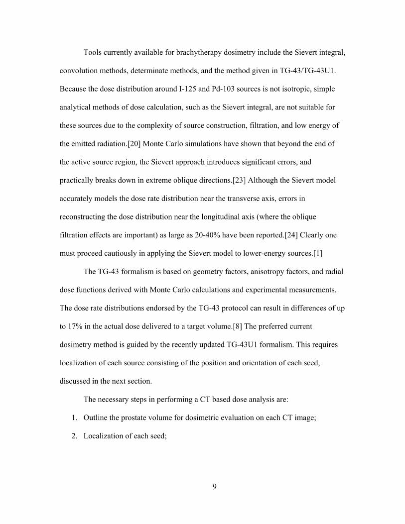
2.6 Simulated Brachytherapy Seed Preparation
Simulated brachytherapy seeds were constructed using stainless steel needles
(Figure 2). The eighteen-gauge needle (nominal outer diameter—1.27 mm, nominal
inner diameter—0.838 mm, nominal wall thickness—0.203 mm) was filled with a small
amount of fluorine-18 (F-18). Seeds were prepared by crimping one needle end before
inserting a smaller needle to deposit the FDG solution from the bottom up, displacing air.
Figure 2. Simulated brachytherapy seeds.
Once the solution was visible at the needle top, another crimp sealed the seed top at
approximately 5 mm long. The needle was snipped at the crimps to complete seed
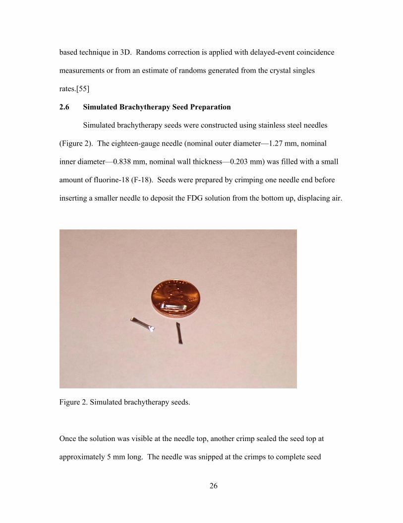
26
construction. The seed was then assayed in the PET hot lab well counter. The activity
and time were recorded for each seed before it was placed in a uniquely numbered tray
slot (Figure 3). After seed construction, all tools were surveyed for potential
contamination. The metal snips exhibited over 500 counts per minute. The snips and
phantom, containing the simulated seeds, were stored in the hot lab after imaging for the
F-18 to decay.
Figure 3. Simulated brachytherapy seed preparation.
2.7 Characteristics of the F-18 Positron Source
The positron emitter used for this study was F-18. F-18 has a half-life of 1.83
hours (110 minutes), a maximum energy of 0.645 MeV, and a branching ratio of 0.967.
F-18 source activity multiplied by the branching ratio yields the positron activity. The
27
positron range from the original emission point to the annihilation depends on its kinetic
energy and on the atomic number of traversed material.[48] PET resolution is inherently
limited by the finite positron range and the fact that the angular separation of two
annihilation photons is not quite 180°.[58] In fact, the electron-positron center of mass
cannot be at rest; for this reason, the two 511 keV photons will be emitted with a relative
angle within 0.25° of 180°, determined by mass and energy conservation.[48]
With a nominal wall thickness of 0.203 mm the probability of an F-18 positron
emerging from the stainless steel needle is very small. In water, the positrons emitted by
F-18 nuclei (maximum energy of 0.645 MeV) have a range less than one millimeter. The
contribution to the final spatial resolution is assessed as FWHM of the count distribution
due to positron range effect, only resulting in a minimal value of 0.2 mm for F-18 in
tissue.[48] The positron decay energy spectrum is similar to that of electrons with an
average energy of approximately one third of the maximum energy, with relatively few
positrons emitted with close to the maximum energy. Charged particles slow down as
they deflect and lose energy. Effective path lengths are derived based on the continuous
slowing down approximation (CSDA).[59] The values for CSDA range and material
density were obtained from ICRU Report 37 “Stopping Powers for Electrons and
Positrons.”[60] There was no data available for positrons in stainless steel so the electron
data for iron was utilized. There are differences arising between positron and electron
energy transfers because an electron can lose at most half its energy in a single collision,
but a positron can lose its entire energy. These differences are derived in terms of a
positron to electron range ratio determined for a few materials. For this calculation the
closest material to iron (Z = 26) with available ratio data was copper (Z = 29). Once a
28
maximum energy positron traverses the seed wall, its residual energy gives rise to a range
of approximately 0.03 mm in water. Therefore the positron range blurring effect due to
the positrons originating inside the seed should have a negligible range outside the seed.
Clearly almost all annihilations will take place within the F-18 solution or the seed
encapsulation.
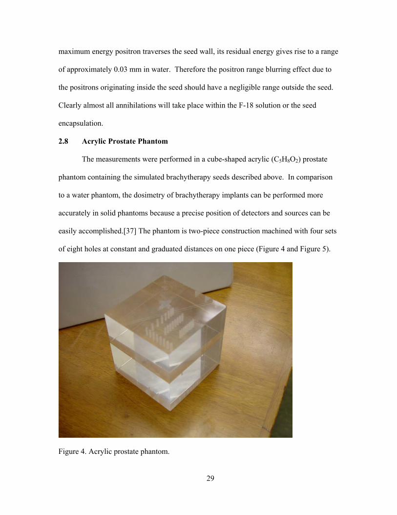
2.8 Acrylic Prostate Phantom
The measurements were performed in a cube-shaped acrylic (C5H8O2) prostate
phantom containing the simulated brachytherapy seeds described above. In comparison
to a water phantom, the dosimetry of brachytherapy implants can be performed more
accurately in solid phantoms because a precise position of detectors and sources can be
easily accomplished.[37] The phantom is two-piece construction machined with four sets
of eight holes at constant and graduated distances on one piece (Figure 4 and Figure 5).
Figure 4. Acrylic prostate phantom.
29

All holes are the same depth and the longitudinal axes of the seeds are parallel. Holes
without seeds were filled with water prior to imaging.
Figure 5. Acrylic prostate phantom on Discovery ST scanner bed.
2.9 Experimental Measurements
The PET/CT measurement started with a scout scan consisting of an x-ray image
overview of the phantom (Figure 6). The resulting scan was displayed for the operator to
define the axial examination range. The axial extent of the CT and PET portions of the
combined scans were matched to ensure fully quantitative attenuation and scatter
correction of the emission data.[47] For the 9 cm long phantom the scanner imposed the
minimum axial distance of 15.7 cm with collection of 47 images each with a slice
thickness of 3.27 mm. Following the definition of imaging range, the phantom moved
30

Figure 6. Phantom aligned with positioning lasers prior to image acquisition.
automatically into the CT field of view for the transmission scan. After completing the
CT scan the phantom advanced to the rear of the combined gantry into the PET field of
view for emission acquisition. Upon completion of the scans and reconstruction, PET
and CT images were transferred to compact disk media; the images are stored in DICOM
(Digital Imaging and Communications in Medicine) format. The stored images consisted
of a CT scan set and both attenuation corrected and non-attenuation corrected PET scan
sets for each slice.
In this study we collected two different data sets. There are some general points
that apply to all scans. The phantom orientation was the same for all images. Image
pixel size depends on the field of view and reconstruction matrix size. The two sets of
scans were acquired with consistent Z placement for all scans by aligning the laser with
31

the joining plane of the two phantom pieces. However, there was some lateral shift
within the first set of scans that was corrected by shifting the data set by the distance
confirmed with seed locations in corresponding CT scans. For the second scan set
phantom alignment marks insured consistent alignment in all three directions.
2.10 Scan Set One—Six Acquisitions
Three seeds were constructed for the first scan set. They were designated as Seed
One, Seed Two, and Seed Three, with activities of 9.0, 3.0, and 6.0 µCi respectively. The
first scan set consisted of three different seed configurations detailed in Table 1.
Table 1. Three seed arrangement composition and seed locations used for scans.
Seed Configuration
Seed One X = 0 mm, Y = 0 mm
Seed Two X = 5 mm, Y = 0 mm
Seed Three X = 30 mm, Y = -15 mm
One Yes No No Two Yes Yes No
Three Yes Yes Yes
For all three seed configurations in scan set one, two-dimensional and three-
dimensional acquisitions were obtained with default image reconstruction, for a total of
six acquisitions. The 2-D and 3-D image acquisitions were conducted consecutively for
each seed configuration without disturbing the phantom. Table 2 summarizes the
acquisition parameters for the six acquisitions of scan set one. Figure 7 shows the seed
arrangements.
Table 2. Acquisition parameters for Scan Set One.
Acquisition 1 Seed Configuration One Protocol PET.CT 2D Body. FEET .In Attenuation Correction CT Scan
CT AC FEET IN--140 kvp, 150 ma, 1121ms, 50 cm FOV, pixel size 0.977 mm, matrix size 512x512
(table continued)
32

PET Series Description PET SLICES IR MAC 2D Acquisition 60 cm FOV, pixel size 4.69 mm, matrix size 128x128 Reconstruction Method OSEM Acquisition 2 Seed Configuration One Protocol PET.CT 2D Body. FEET .In Attenuation Correction CT Scan
CT AC FEET IN--140 kvp, 150 ma, 1121ms, 50 cm FOV, pixel size 0.977 mm, matrix size 512x512
PET Series Description PET SLICES 3D MAC 3D Acquisition 60 cm FOV, pixel size 2.34 mm, matrix size 256x256 Reconstruction Method 3D FORE IR Acquisition 3 Seed Configuration Two Protocol PET.CT 2D Body. FEET .In Attenuation Correction CT Scan
CT AC FEET IN--140 kvp, 100 ma, 1018ms, 50 cm FOV, pixel size 0.977 mm, matrix size 512x512
PET Series Description PET SLICES IR MAC 2D Acquisition 60 cm FOV, pixel size 4.69 mm, matrix size 128x128 Reconstruction Method OSEM Acquisition 4 Seed Configuration Two Protocol PET.CT 2D Body. FEET .In Attenuation Correction CT Scan
CT AC FEET IN--140 kvp, 100 ma, 1018ms, 50 cm FOV, pixel size 0.977 mm, matrix size 512x512
PET Series Description PET SLICES 3D AC 3D Acquisition 60 cm FOV, pixel size 2.34 mm, matrix size 256x256 Reconstruction Method 3D FORE IR Acquisition 5 Seed Configuration Three Protocol PET.CT 2D Body. FEET .In Attenuation Correction CT Scan
CT AC FEET IN--140 kvp, 100 ma, 1018ms, 50 cm FOV, pixel size 0.977 mm, matrix size 512x512
PET Series Description PET SLICES IR MAC 2D Acquisition 60 cm FOV, pixel size 4.69 mm, matrix size 128x128 Reconstruction Method OSEM Acquisition 6 Seed Configuration Three Protocol PET.CT 2D Body. FEET .In Attenuation Correction CT Scan
CT AC FEET IN--140 kvp, 100 ma, 1018ms, 50 cm FOV, pixel size 0.977 mm, matrix size 512x512
PET Series Description PET SLICES 3D MAC 3D Acquisition 60 cm FOV, pixel size 2.34 mm, matrix size 256x256 Reconstruction Method 3D FORE IR
33

Figure 7. Scan Set One CT (top) and PET (bottom) images located at Z = 0 (ezDICOM viewer).
2.11 Scan Set Two—Four Acquisitions
Three seeds were constructed for the second scan set. They were designated as
Seed Four, Seed Five and Seed Six with activities of 4.6, 4.9, and 4.5 µCi respectively.
The second scan set consisted of the same three different seed configurations in scan set
one listed in Table 1. For all three seed configurations of the second scan set, 2D whole
body protocol were acquired. In addition, for seed configuration one, a 2D brain or heart
protocol was used. Each of these four acquisitions was reconstructed with both 128x128
and 256x256 matrix sizes for a total of eight reconstructed data sets from scan set two.
Table 3 summarizes the acquisition parameters for scan set two.
34
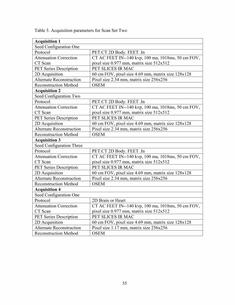
Table 3. Acquisition parameters for Scan Set Two
Acquisition 1 Seed Configuration One Protocol PET.CT 2D Body. FEET .In Attenuation Correction CT Scan
CT AC FEET IN--140 kvp, 100 ma, 1018ms, 50 cm FOV, pixel size 0.977 mm, matrix size 512x512
PET Series Description PET SLICES IR MAC 2D Acquisition 60 cm FOV, pixel size 4.69 mm, matrix size 128x128 Alternate Reconstruction Pixel size 2.34 mm, matrix size 256x256 Reconstruction Method OSEM Acquisition 2 Seed Configuration Two Protocol PET.CT 2D Body. FEET .In Attenuation Correction CT Scan
CT AC FEET IN--140 kvp, 100 ma, 1018ms, 50 cm FOV, pixel size 0.977 mm, matrix size 512x512
PET Series Description PET SLICES IR MAC 2D Acquisition 60 cm FOV, pixel size 4.69 mm, matrix size 128x128 Alternate Reconstruction Pixel size 2.34 mm, matrix size 256x256 Reconstruction Method OSEM Acquisition 3 Seed Configuration Three Protocol PET.CT 2D Body. FEET .In Attenuation Correction CT Scan
CT AC FEET IN--140 kvp, 100 ma, 1018ms, 50 cm FOV, pixel size 0.977 mm, matrix size 512x512
PET Series Description PET SLICES IR MAC 2D Acquisition 60 cm FOV, pixel size 4.69 mm, matrix size 128x128 Alternate Reconstruction Pixel size 2.34 mm, matrix size 256x256 Reconstruction Method OSEM Acquisition 4 Seed Configuration One Protocol 2D Brain or Heart Attenuation Correction CT Scan
CT AC FEET IN--140 kvp, 100 ma, 1018ms, 50 cm FOV, pixel size 0.977 mm, matrix size 512x512
PET Series Description PET SLICES IR MAC 2D Acquisition 60 cm FOV, pixel size 4.69 mm, matrix size 128x128 Alternate Reconstruction Pixel size 1.17 mm, matrix size 256x256 Reconstruction Method OSEM
35

2.12 Extracting Annihilation Event Density From PET DICOM Files
Three free DICOM readers, Osiris, MRIcro, and ezDICOM were used for viewing
the DICOM format images. IDL 5.6 Student Edition (Research Systems, Inc.) and Visual
Basic 6.0 (Microsoft Corporation) were used to process the PET image data.
IDL was used to read the pixel data from an image file and multiply each data
point by the image scale factor to generate a raw output data file. A Visual Basic
program was then used to locate within the output data file the pixel with the maximum
pixel value and to extract sub-sets of pixels based on the location and magnitude of this
reference point. The reference element for all studies was the seed located at the
phantom center. The single seed in scan set one had the highest activity of the three
seeds at 9 µCi. This pixel was easy to locate in the PET data because it had the largest
value. A shift in X-Y location of the largest pixel value was noted between the one and
two seed cases. Checking the CT scans of each case revealed that the location of the
reference seed had been shifted between the two acquisitions. Even though the Z
alignment was identical for all scans, the phantom was aligned in a slightly different X-Y
location for these scans. The magnitude of shift was identified in the CT scan and the
reference point was shifted to match the MCNP source input locations and corresponding
raw data probability distributions.
2.13 Data Reduction for MCNP Input—Pixel Data Significance
The Sajo and Williams technique links the therapy dose distribution to the dose
distribution due to the annihilation photons.[3] The goal of this research is to test the
hypothesis that the scanner output can be utilized to calculate the annihilation dose
distribution. While estimated true counts or activity concentration would be logical units
36
for raw scanner output, the actual format isn’t important as long as the relative data is
intact. The assumption we are making is that the difference between the raw output data
and the actual activity concentration is only a scaling factor. Therefore, the scanner raw
output data maintains the integrity of the relative activity of each voxel. A voxel is a
three-dimensional volume element analogous to a two-dimensional pixel. The voxel
volume is determined by the image slice thickness and pixel size.
The raw GE PET/CT scanner output data is used for MCNP input. The raw
output value reported for each voxel is entered into MCNP source input as the relative
probability of photon emission per voxel. Because the computational results are
normalized to one photon source, the results of both the theoretical ideal source
distribution and the source distribution from the experimentally measured data can be
directly compared. Furthermore, at some point in the future when sources of known
strength are utilized, the activity of those sources can be used with the MCNP calculated
dose distribution using scanner output for source, normalized to one photon, for mapping
the actual dose distribution due to the annihilation photons.
Not all of the raw scanner output data is significant for MCNP input. PET images
are formulated with data containing false information due to contributions from intrinsic
properties such as scatter and noise. There are also large blocks of the PET data that have
zero values and clearly all data is not significant for input. In examining the question of
what data is significant, results of different input data sets will be compared. The
Discovery ST acquires a minimum of forty-seven slices combined with the smallest
matrix size of 128x128 results in 770,048 voxels. An initial attempt to analyze all
available input data resulted in over one million input lines crashing MCNP5. Two
37

factors were considered for eliminating insignificant input data: the slice scaling factor
and positron range. Comparing the scaling factors of adjacent slices revealed that all data
within three orders of magnitude was within four slices above and four slices below the Z
= 0 slice. Nine slices of data, the central one and four from each side, would contain all
data within three orders of magnitude of the maximum pixel value. Finally, based on the
positron range calculation, using five slices of input data includes the voxels that could
contain the seeds plus a one voxel margin. Using five slices of data would easily account
for the maximum positron range. Both the nine slice dataset and the five slice dataset
were compared to the theoretical distribution.
38

CHAPTER 3
MCNP5 COMPUTATIONAL EXPERIMENTS
3.1 Introduction
Historically Monte Carlo methods have played an important role in computational
dosimetry. MCNP5 (Monte Carlo N-Particle, version 5) is a particle transport computer
code with powerful three-dimensional combinatorial geometry and source modeling
capabilities that can be applied to various fields, including medical physics.[62, 63]
MCNP5 utilizes the frequently updated ENDF/B-VI (Evaluated Nuclear Data File,
Release B, version VI) cross-section library and models combined neutron, photon, and
electron transport, including secondary photon and electron/positron creation. MCNP5
has been widely validated against experimental measurements and benchmarked using
other codes, so that its operating parameters and limitations are well understood.[62-64]
Monte Carlo codes provide a means of constructing an idealized reality for theoretical
experiments far from the clinical environment. Although Monte Carlo studies are free
from experimental artifacts such as positioning uncertainties, energy response
corrections, and signal-to-noise ratio limitations, such simulations require an accurate and
complete geometric model of the source, selection of appropriate cross section library,
and careful selection of dose tallying and variance reduction strategies.[5] MCNP5 has
been widely used for interstitial brachytherapy dosimetry.[65] For the purpose of this
study, MCNP5 for WindowsTM was obtained from the Radiation Safety Information
Computational Center (www-rsicc.ornl.gov) for free; however, there are security
restrictions on obtaining and using the software package. In this project, MCNP5 was
utilized for the calculation of energy deposition in tallied voxels due to the 511 keV
39

photons from both the theoretical and measured positron annihilation distributions.
Because MCNP is a widely known and accepted code, if done correctly the results should
be considered meaningful and significant. All calculations were performed on a Pentium
4 CPU running at 2.80 GHz equipped with 448 MB of RAM.
3.2 Simulation of Seed Geometry Dose Deposition
Because the investigator performing Monte Carlo analysis can control many
features of the transport calculations, it is imperative that the salient details be
described.[5] In the rest of this chapter the specific features of the MCNP inputs used for
this study are explained. Monte Carlo simulation must be used with caution. The
accuracy of the estimated energy deposition is highly dependent on the accuracy of the
source construction and geometry construction.[5] Certain features were used universally
so these will be explained before moving on to unique input file specific parameters.
Some general considerations for all MCNP related work in this study: problem geometry
was not set up all at once, small steps were taken as the input progressed with literally
hundreds of MCNP runs because each small change in input was verified, short job
output statistics and reasonableness were examined carefully, the simplest geometry and
source were chosen without sacrificing accuracy, all geometry was plotted using the
visual editor to identify geometric problems, and all MCNP5 warning messages were
investigated for each computational experiment.
The tally utilized in our simulation was the energy deposition in units of MeV per
voxel for both photons and electrons. In MCNP, this tally is the pulse-height distribution
in the detectors modified to energy times the weight (designated in MCNP as *F8:p,e in
lattice form).
40

The modeled physical geometry included the void, air, phantom, and seeds
(Figure 8). The void consisted of all space outside the green sphere with radius 10 cm
centered at the origin for all runs. Outside the phantom, but within the 10 cm radius
sphere, was air for all runs. The computational description of the phantom followed the
dimensions of the real one and was identical in all runs except for the seed positions. The
acrylic prostate phantom was represented by water, but the difference should be small for
our case with 511 keV photons, as the difference in the mass interaction coefficients of
these respective materials is demonstrated for 500 keV photons in Table 4.
The phantom was centered in the X and Y directions and measured a total of 9 cm
in both the X and Y directions. The phantom length in Z direction was 8.8 cm and the Z
= 0 plane was perpendicular to the longitudinal axis of the seed intersecting it at the seed
center, corresponding to 5.7 cm down from the positive Z phantom surface and 3.1 cm up
from the negative Z phantom surface. The simulated brachytherapy seeds were
constructed with iron to represent stainless steel. The seeds are all the same size and
shape consisting of the union of space between two cylinders with four planes for the
ends—two defining the seed top and two defining the seed bottom. The composition and
mass density of materials incorporated in all input files were exactly the same. Materials
utilized for input are listed in Table 5.
Table 4. Mass interaction coefficients listed for Water, Acrylic, and Tissue (ICRU 33
four component definition) for 500 keV photons. Material µ/ρ g/cc Weight Fraction Water 0.09664 1.00 H 0.111894, O 0.888106 Acrylic 0.09393 1.19 H 0.080541, C 0.599846, O 0.319613 Tissue 0.09572 1.00 H 0.101174, C 0.111000, N 0.026000, O 0.761826
41

Figure 8. One Seed in Phantom with X-Z tally voxels (red) 128x128 matrix size with
4.69 mm pixel size and 3.27 slice thickness that corresponds to the GE Discovery ST PET/CT scanner used in this study.
Table 5. Material composition and mass density for materials used in MCNP input
(courtesy of Bristol-Myers Squibb Medical Imaging). Material Element Weight Fraction Adult Tissue Hydrogen 0.10454 Density = 1.04 g/cc Carbon 0.22663 Nitrogen 0.02490 Oxygen 0.63525 Sodium 0.00112 Magnesium 0.00013 Silicon 0.00030 Phosphorus 0.00134 Sulfur 0.00204 Chlorine 0.00133 Potassium 0.00208 Calcium 0.00024 Iron 0.00005
(table continued)
42
Zinc 0.00003 Rubidium 0.00001 Zirconium 0.00001 Water Hydrogen 0.11189 Density = 1.00 g/cc Oxygen 0.88810 Air Carbon 0.00012 Density = 0.001020 g/cc Nitrogen 0.75527 Oxygen 0.23178 Argon 0.01283 Iron Iron 1.00000 Density = 7.86 g/cc
3.3 Annihilation Source Geometry in the MCNP Simulation
Source specification may be the most difficult and complicated part of MCNP
input. The accuracy of Monte Carlo is inherently limited by the investigators’ ability to
accurately delineate the source internal geometry.[5] Although it can transport positrons
as secondary particles, MCNP5 does not support positrons as source particles. Therefore
no radioisotopes were used as sources for the MCNP5 theoretical experiments in this
research. All source particles were 511 keV photons meant to represent positron
annihilation events from the F-18. For the theoretical distributed source, photons
originate at a random position and direction within the seed wall where we have shown
that almost all positron annihilation events occur. For the PET/CT measured distribution,
a point source at the center of each voxel was assigned a probability based on the PET
scanner raw output extracted from the DICOM format file. Both source distributions
were verified with MCNP print table 110 that lists the starting location and direction of
the first fifty histories. All events originating within a particular volume element cannot
be distinguished based on location. The three source geometries considered for this work
(within one voxel) were point, line, and volume. A point source at the voxel center
would emit 511 keV photons with a frequency based on the relative intensity measured
43

with the PET scanner. The line source is oriented in the Z direction, similar to the seed,
and homogenized over the entire length with a frequency of photon emission again based
on the scanner measurements. The volume source would consist of random starting
locations and directions from within the entire voxel element. After careful
consideration, the point source at voxel center was finally selected over the line or
volume source. A comparison of homogenized versus point source was done in a
separate set of computational experiments detailed below, but this was not done for the
line source due to time constraints. Using a point source at the voxel center is the most
practical choice resulting in reduced running time and reasonable input complexity.
To insure that using point sources at the center of each voxel would not result in
significant error, energy deposition from a uniform arrangements of voxel volume
sources were compared to the energy deposition from a uniform arrangement of point
sources at the center of each corresponding voxel. The resulting energy deposition in
each voxel was tallied for comparison along the Z-axis, but only within the source
volume. After further review of the results, another group of computations was
conducted to examine the resulting dose distribution throughout the entire phantom as
well. We wanted to investigate the higher dose gradient regions on the periphery of
source arrangements and the correspondence of dose deposition between the point and
volumetric source cases extending outwards from the treatment volume. Computations
were conducted for small volumes on the order of one-voxel source up to comparatively
much larger volume sources up to 15 x 15 x 15 voxels. We expected that the discrepancy
between point and volume sources would be the greatest for a small volume source, and
smallest for a larger volume source, approximating the size of the prostate. For larger
44

three-dimensional arrays, the difference between using a point source at the center of
each voxel instead of a uniformly distributed array of voxel volume sources was close
and well within the error reported by MCNP5. The next chapter shows a comparison of
computed dose depositions between point sources versus volume sources for the larger
volume case.
3.4 MCNP5 Energy Deposition Calculation Experiments
A summary list of the forty-nine MCNP5 computational experiments performed
in the course of this research is given in Appendix A. Experiments 1 through 7
demonstrate theoretical seed source distributions; experiments 8 through 27 depict energy
distributions due to voxel volume sources and arrangements of point sources at the center
of those voxels; experiments 28 through 39 are for measured source data from Scan Set
One; experiments 40 through 49 represent measured source data from the Scan Set Two.
The experimental results are shown and discussed in Chapter 4.
3.5 MCNP5 Uncertainty Analysis
The statistical error, or uncertainty, associated with the result is equal in
importance to the Monte Carlo tally itself. MCNP tallies are normalized per starting
particle and are printed in the output accompanied by a second number representing the
relative standard deviation. At the end of the output file is the tally fluctuation chart
(TFC).[62] The TFC always should be studied to see how stable or reliable are the
estimated mean, relative error (R), variance of the variance (VOV), figure of merit
(FOM), and the slope of the largest history scores which are indicative of how the
solution is converging as the number of photon histories, NPS.
45

CHAPTER 4
RESULTS AND CONCLUSIONS
4.1 Introduction
Sajo and Williams developed a theoretical correspondence between the dose
distributions due to the therapy dose and to a trace amount of positron emitter
encapsulated within the seeds utilized in prostate brachytherapy implants.[3] The main
aim of this research is to ascertain if PET image data of a positron tracer can be used for
the quantitative description of dose distribution in support of direct prostate seed
dosimetry. To do this, we compared the dose distribution due to the 511 keV photons
calculated from the annihilation event distribution of experimental measurements of
mock brachytherapy seeds to a computer-modeled distribution of ideal positron emitting
seeds. If clinically implemented, this dosimetric technique could improve the accuracy,
reproducibility, and complexity of absorbed dose calculations due to implanted sources.
The results of this study are divided into three sections. The first section provides the
experimental and computational results, the second section is a discussion of the results,
and the final section draws conclusions from the results and discussion.
4.2 Results
This section examines the Monte Carlo calculated dose distributions for the
measured versus theoretical activity distributions. Furthermore, the results due to the
acquisition mode, reconstruction method, and maximum error bound are reported.
Lastly, the results for the point versus volume source simulations are given.
The results shown in Figures 9-14, as well as all figures in Appendix B, depict the
Monte Carlo calculated energy deposition in individual voxel volume elements. As
46

shown in Figure 8, the energy deposition was tallied in voxel arrays on the longitudinal
and transverse phantom axis. We studied the energy deposited per voxel because the
desired dose determination grid is based on the PET data reported per voxel. The dose
distribution is obtained by dividing the energy deposition by the corresponding voxel
mass. All graphs include error bars representing the statistical error ±1σ of Monte Carlo
calculations. Appendix B provides a complete set of the Monte Carlo calculation results
not summarized in this chapter, in both tabular and graphical form.
Examination of the energy distributions indicates a small disagreement between
the computed doses based on the measured data versus theoretical sources for certain
cases. In particular, the agreements for the one and two seed cases were close.
For the one seed case, as shown in Figure 9, we found that 2D acquisition with
OSEM reconstruction resulted in a maximum difference in transaxial dose distribution of
15% in voxel two, and a mean difference of 4% for the remaining voxels. The mean
discrepancy between dose computations based on the ideal source versus PET based
source is within or close to the Monte Carlo error of 2% to 4%.
For the two seed case, as shown in Figure 10, we found that 2D acquisition with
OSEM reconstruction resulted in a maximum difference in transaxial dose distribution of
16% in voxel one, and a mean difference of 2% for voxels two through six. The mean
discrepancy between dose computations based on the ideal source versus PET based
source is within or close to the Monte Carlo error of up to 3.5%.
The results of Seed Arrangement Three are depicted in Figure 11, and consisted
of two seeds together and one seed farther out as explained in Table 1 found in section
2.10. In pursuit of thoroughness we wanted to see if the proximal range of seeds had
47
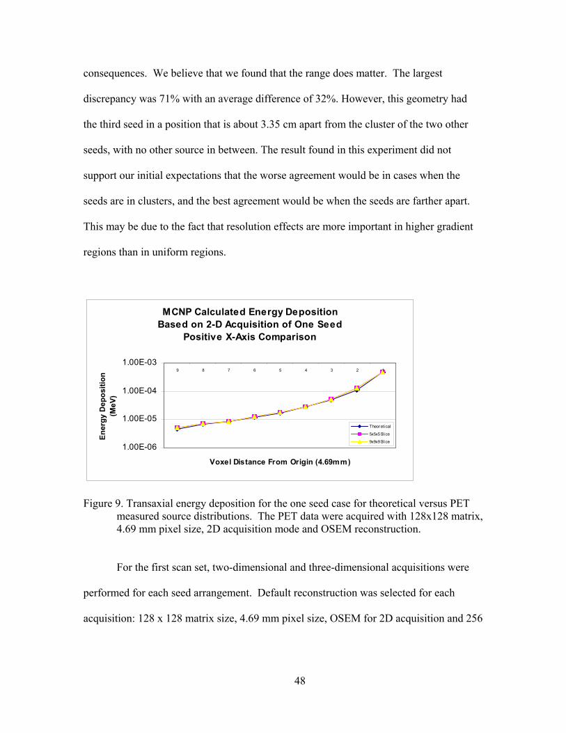
consequences. We believe that we found that the range does matter. The largest
discrepancy was 71% with an average difference of 32%. However, this geometry had
the third seed in a position that is about 3.35 cm apart from the cluster of the two other
seeds, with no other source in between. The result found in this experiment did not
support our initial expectations that the worse agreement would be in cases when the
seeds are in clusters, and the best agreement would be when the seeds are farther apart.
This may be due to the fact that resolution effects are more important in higher gradient
regions than in uniform regions.
MCNP Calculated Energy DepositionBased on 2-D Acquisition of One Seed
Positive X-Axis Comparison
1.00E-06
1.00E-05
1.00E-04
1.00E-039 8 7 6 5 4 3 2 1
Voxel Distance From Origin (4.69mm)
Ener
gy D
epos
ition
(M
eV)
Theor etical
5x5x5 Sl ice
9x9x9 Sl ice
Figure 9. Transaxial energy deposition for the one seed case for theoretical versus PET measured source distributions. The PET data were acquired with 128x128 matrix, 4.69 mm pixel size, 2D acquisition mode and OSEM reconstruction.
For the first scan set, two-dimensional and three-dimensional acquisitions were
performed for each seed arrangement. Default reconstruction was selected for each
acquisition: 128 x 128 matrix size, 4.69 mm pixel size, OSEM for 2D acquisition and 256
48
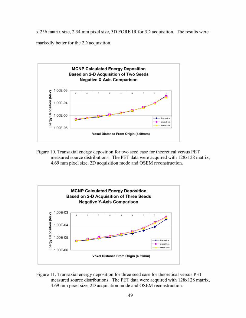
x 256 matrix size, 2.34 mm pixel size, 3D FORE IR for 3D acquisition. The results were
markedly better for the 2D acquisition.
MCNP Calculated Energy DepositionBased on 2-D Acquisition of Two Seeds
Negative X-Axis Comparison
1.00E-06
1.00E-05
1.00E-04
1.00E-039 8 7 6 5 4 3 2 1
Voxel Distance From Origin (4.69mm)
Ener
gy D
epos
ition
(MeV
)
Theoretical
5x5x5 Slice
9x9x9 Slice
Figure 10. Transaxial energy deposition for two seed case for theoretical versus PET measured source distributions. The PET data were acquired with 128x128 matrix, 4.69 mm pixel size, 2D acquisition mode and OSEM reconstruction.
MCNP Calculated Energy DepositionBased on 2-D Acquisition of Three Seeds
Negative Y-Axis Comparison
1.00E-06
1.00E-05
1.00E-04
1.00E-039 8 7 6 5 4 3 2 1
Voxel Distance From Origin (4.69mm)
Ener
gy D
epos
ition
(MeV
)
Theoretical
5x5x5 Slice
9x9x9 Slice
Figure 11. Transaxial energy deposition for three seed case for theoretical versus PET measured source distributions. The PET data were acquired with 128x128 matrix, 4.69 mm pixel size, 2D acquisition mode and OSEM reconstruction.
49

Compared to the close correlation of the one seed case above, looking at graph for
3D acquisition of the same single seed in Figure 12 shows obvious disparity in the result
close to the seed that was found to be 65% different in voxel one, and 22% in voxel two.
However, the next eleven dose positions exhibit a relatively good agreement with a mean
difference of 3%. These results could be because 3D acquisition is known to have more
scatter and randoms, overall poorer resolution, but higher sensitivity. The potential
benefit of using 3D mode is that collecting many more lines of response requires less
radioactivity with the dual benefit of reduced patient exposure and needing a reduced
quantity of radiotracer.
A brain acquisition protocol was performed during the second set of scans. As it
is in Figure 13, the brain protocol was not nearly as close to the theoretical distribution as
the whole body protocol, showing large discrepancies from voxels 2 through 5.
MCNP Calculated Energy DepositionBased on 3-D Acquisition of One Seed
Positive X-Axis Comparison
1.00E-06
1.00E-05
1.00E-04
1.00E-0318 17 16 15 14 13 12 11 10 9 8 7 6 5 4 3 2 1
Voxel Distance From Origin (2.34 mm)
Ener
gy D
epos
ition
(MeV
)
Theoretical
9x9x5 Slice
17x17x9 Slice
Figure 12. Transaxial energy deposition for one seed case for theoretical versus PET measured source distributions. The PET data were acquired with 256 x 256 matrix, 2.34 mm pixel size, 3D acquisition mode and 3D FORE IR reconstruction.
50

For the Scan Set Two, all acquisitions were two-dimensional, however there was
a question if the results could be improved by an alternate image reconstruction matrix
and voxel size. The Scan Set Two acquisitions were reconstructed with OSEM
consisting of 128 x 128 matrix with 4.69 mm voxel size and one step smaller voxel size,
256 x 256 matrix with 2.34 mm voxel size, as seen in Figure 12. We found that the
default 128 x 128 matrix size reconstruction with 4.69 mm voxel size provided the
closest results in all cases.
MCNP Calculated Energy Deposition2-D Acquisition 128x128 Recon Second Scan
One Seed Positive X-Axis Comparison
1.00E-06
1.00E-05
1.00E-04
1.00E-039 8 7 6 5 4 3 2 1
Voxel Distance From Origin (4.69mm)
Ener
gy D
epos
ition
(MeV
)
Theoretical
Whole Body
Brain
Figure 13. Transaxial energy deposition for one seed case for theoretical versus PET measured source distributions. The PET data were acquired with 128 x 128 matrix, 4.69 mm pixel size, 2D acquisition with Whole Body and Brain protocols and OSEM reconstruction.
Because we don’t know the precise seed location within the voxel, there is some
uncertainty in assigning the voxel activity to the voxel center. Because we assigned the
largest voxel value to the voxel containing the seed, the seed could be located anywhere
within that voxel. We wanted to determine that our results were consistent with this
assumption, so calculations were performed with the source data shifted by one half
51

voxel in both the positive X and negative X directions. All graphed values are within
these limits that could be due to the assumption of placing the seed in the center of the
voxel. Because a half-voxel was the maximum possible shift due to our assumption, this
represents the maximum error bound due to this assumption. The results we obtained
were within this outer-bound. Our result did indeed fall within the maximum and
minimum values found due to these shifts seen in Figure 14.
MCNP Calculated Energy Deposition2-D Acquisition 128x128 Max Error
Positive X-Axis Comparison
1.00E-06
1.00E-05
1.00E-04
1.00E-039 8 7 6 5 4 3 2 1
Voxel Distance From Origin (4.69mm)
Ener
gy D
epos
ition
(MeV
)
Voxel Center
Negative Shift
Positive Shift
Figure 14. Transaxial energy deposition for one seed case for PET measured source distributions located at the voxel center versus data shifted one-half voxel distance in the positive and negative X directions. The PET data were acquired with 128 x 128 matrix, 4.69 mm pixel size, 2D acquisition with Whole Body and Brain protocols and OSEM reconstruction.
Finally, several Monte Carlo calculations were performed to insure that using an
array of point sources located at each voxel center would not significantly alter the tally
results. We expect that the dose within an array of seeds can be well approximated by
using point sources. This approximation should be largest at the perimeter of the array.
Initially only the internal part of the array was tallied, but after further review of the data,
52

a decision was made to tally all voxels from the origin out to the phantom edge in another
set of calculations. This would allow us to see how the deposited energy varied from
inside the source region, through and beyond the array boundary.
A number of source arrays were considered, starting with the simplest case of a
single source. The studies comparing the energy deposition for inside the source region
was tallied along the Z-axis. The largest discrepancy was, as expected, for the single
voxel distributed volume source versus a single point source at the voxel center. Similar
studies were performed for 3 x 3 x 3, 5 x 5 x 5, 7 x 7 x 7, and 15 x 15 x 15 voxels
measuring 2 mm on each side. Table 6 summarizes the voxel arrangement. The infinite
arrangement was achieved by using reflective boundaries in the computations.
Table 6. Point versus volume source study cases.
Case Voxel Arrangement Point Sources (Voxel Center) 1 1 1 2 3 x 3 x 3 27 3 5 x 5 x 5 125 4 7 x 7 x 7 343 5 15 x 15 x 15 3375 6 Infinite Infinite
As expected, the single distributed source versus single point source case
provided the largest discrepancy in energy deposition within the source voxel of 34.87%.
The internal results for all but the point source are illustrated in the Figures 15 and 16,
with Figure 16 showing that for the 15 x 15 x 15 array that the results are within the
Monte Carlo calculation uncertainty. Figure 17 demonstrates the energy deposition
throughout the phantom for the 15 x 15 x 15 distribution.
53
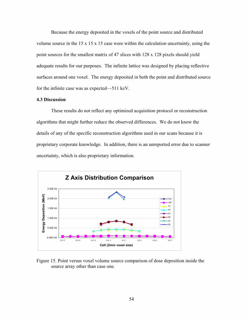
Because the energy deposited in the voxels of the point source and distributed
volume source in the 15 x 15 x 15 case were within the calculation uncertainty, using the
point sources for the smallest matrix of 47 slices with 128 x 128 pixels should yield
adequate results for our purposes. The infinite lattice was designed by placing reflective
surfaces around one voxel. The energy deposited in both the point and distributed source
for the infinite case was as expected—511 keV.
4.3 Discussion
These results do not reflect any optimized acquisition protocol or reconstruction
algorithms that might further reduce the observed differences. We do not know the
details of any of the specific reconstruction algorithms used in our scans because it is
proprietary corporate knowledge. In addition, there is an unreported error due to scanner
uncertainty, which is also proprietary information.
Z Axis Distribution Comparison
0.00E+00
5.00E-05
1.00E-04
1.50E-04
2.00E-04
2.50E-04
0 0 -7 0 0 -5 0 0 -3 0 0 -1 0 0 1 0 0 3 0 0 5 0 0 7
Cell (2mm voxel size)
Ener
gy D
epos
ition
(MeV
)
15V
15P
7V
7P
5V
5P
3V
3P
Figure 15. Point versus voxel volume source comparison of dose deposition inside the source array other than case one.
54
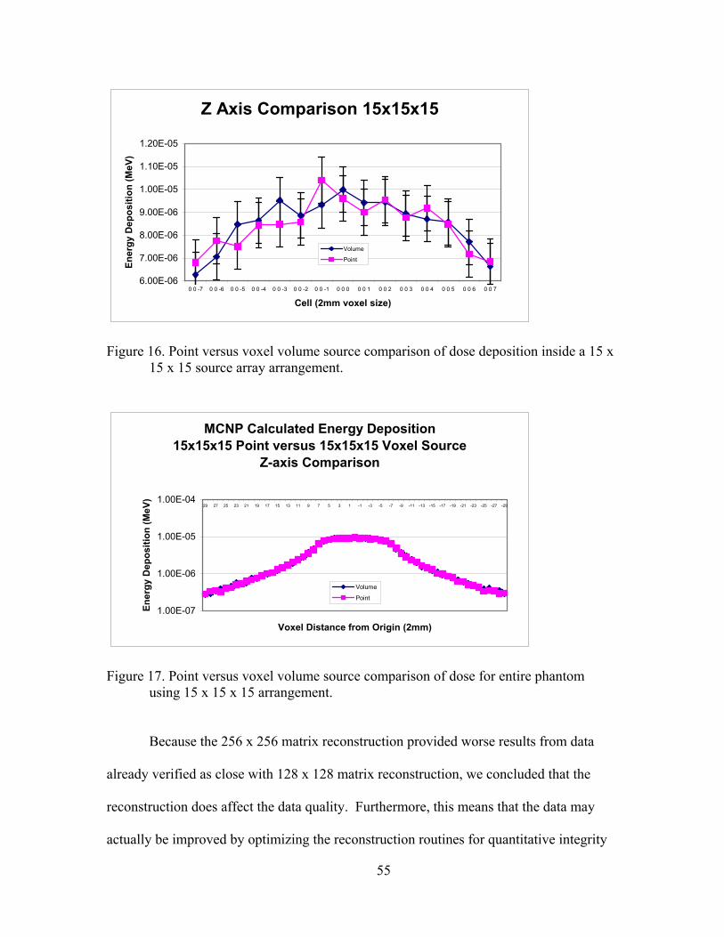
Z Axis Comparison 15x15x15
6.00E-06
7.00E-06
8.00E-06
9.00E-06
1.00E-05
1.10E-05
1.20E-05
0 0 -7 0 0 -6 0 0 -5 0 0 -4 0 0 -3 0 0 -2 0 0 -1 0 0 0 0 0 1 0 0 2 0 0 3 0 0 4 0 0 5 0 0 6 0 0 7
Cell (2mm voxel size)
Ener
gy D
epos
ition
(MeV
)
Volume
Point
Figure 16. Point versus voxel volume source comparison of dose deposition inside a 15 x 15 x 15 source array arrangement.
MCNP Calculated Energy Deposition15x15x15 Point versus 15x15x15 Voxel Source
Z-axis Comparison
1.00E-07
1.00E-06
1.00E-05
1.00E-0429 27 25 23 21 19 17 15 13 11 9 7 5 3 1 -1 -3 -5 -7 -9 -11 -13 -15 -17 -19 -21 -23 -25 -27 -29
Voxel Distance from Origin (2mm)
Ener
gy D
epos
ition
(MeV
)
Volume
Point
Figure 17. Point versus voxel volume source comparison of dose for entire phantom using 15 x 15 x 15 arrangement.
Because the 256 x 256 matrix reconstruction provided worse results from data
already verified as close with 128 x 128 matrix reconstruction, we concluded that the
reconstruction does affect the data quality. Furthermore, this means that the data may
actually be improved by optimizing the reconstruction routines for quantitative integrity
55

since we are not interested in the qualitative or diagnostic use of these images. In several
cases, discrepancies may be due to reconstruction inadequacies such as applying a filter
that is sub-optimal for quantitative optimization. Data can clearly be made worse by
poorly chosen reconstruction parameters, thus it can be also optimized for strictly
quantitative use. If inadequacies were due to bad statistics, we would see worse results
primarily far away from the source. Data are used qualitatively by manufacturers for
visual image analysis, but to optimize the quantitative voxel values may require separate
algorithms. To conduct standardized QA testing, GE can provide generic reconstruction
programs. Data not altered for visual optimization may be even better for our
quantitative use.
The reconstruction parameters (filters, etc.) and their effect on the data are
unknown. Insufficient knowledge about image reconstruction specifics may be
responsible for discrepancies observed in the generated data. Even though the scanner
may opt for a more robust 3D iterative reconstruction, the DICOM files are still
individual slices of 2D information.
Of concern was the significance of outlying counts. An attempt was made to
include all measured events but clearly a cutoff was needed. Because using all slice data
for input crashed MCNP5, we had to determine what input information could be
eliminated with confidence. It has been reported that image blurring caused by scattered
events may lead to important quantification errors. This is complicated by the fact that
advanced nuclear medical imaging systems collect multiple attributes of a large number
of photon events resulting in extremely large datasets which present challenges to image
reconstruction and assessment. We thought data from outside the positron range was
56

false. Because of the short range of F-18 positrons in water, we found that using the
positron range with one extra voxel margin was adequate to remove spurious counts.
This resulted in five slices of data with a corresponding matrix size in the X-Y plane. To
be thorough, while not eliminating so much data to have an effect on our result, we
investigated using a larger range of input based on nine slices with similar increase in x-y
voxel range. The quality of agreement between the five and nine slice inputs is
remarkable. In the Figures 9-12 above, the results for nine and five slices of data are
compared. Practically, there is no appreciable difference between the results. Therefore,
utilizing five slices of data around the seed arrangement appears safe and more reduction
may be possible. By comparing the different input matrices, the positron range appears
reasonable for determining what data could be disregarded with confidence.
There is a very good agreement in the case of increasing numbers of point sources
representing voxel volume sources. For the largest number of tested sources, the
difference is within the Monte Carlo calculation error average of 5%. To insure that a
point source at the center of each voxel would accurately represent the relative activity
for a voxel volume source, several cases were designed and analyzed for comparison.
Even though a point source located at the center was the most practical source for
each voxel, the seed geometry in both the real and theoretical cases is closer to a line
source oriented parallel to the Z-axis. Line sources located at the center of each pixel in
the X and Y direction but extending the entire length of the voxel in the Z direction
parallel to the Z-axis are possible, but provide problems as well. The raw output data
from the PET scanner is assigned to that length with a uniform distribution along the line
throughout that voxel. A line source in that voxel could artificially stretch the activity in
57
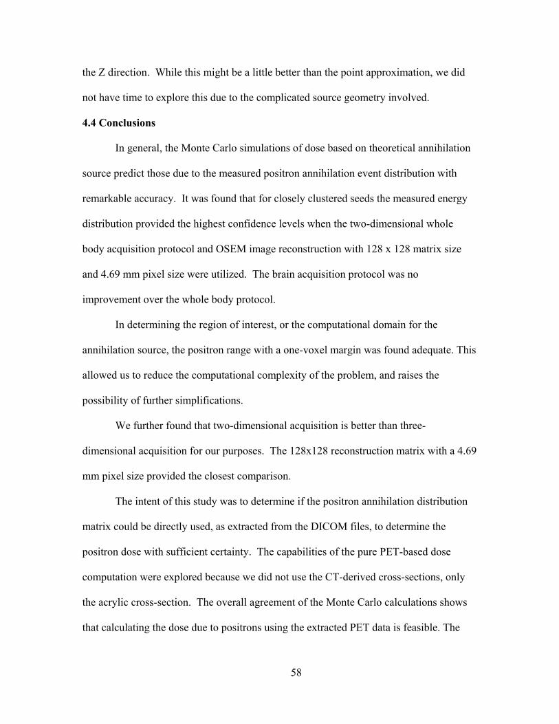
the Z direction. While this might be a little better than the point approximation, we did
not have time to explore this due to the complicated source geometry involved.
4.4 Conclusions
In general, the Monte Carlo simulations of dose based on theoretical annihilation
source predict those due to the measured positron annihilation event distribution with
remarkable accuracy. It was found that for closely clustered seeds the measured energy
distribution provided the highest confidence levels when the two-dimensional whole
body acquisition protocol and OSEM image reconstruction with 128 x 128 matrix size
and 4.69 mm pixel size were utilized. The brain acquisition protocol was no
improvement over the whole body protocol.
In determining the region of interest, or the computational domain for the
annihilation source, the positron range with a one-voxel margin was found adequate. This
allowed us to reduce the computational complexity of the problem, and raises the
possibility of further simplifications.
We further found that two-dimensional acquisition is better than three-
dimensional acquisition for our purposes. The 128x128 reconstruction matrix with a 4.69
mm pixel size provided the closest comparison.
The intent of this study was to determine if the positron annihilation distribution
matrix could be directly used, as extracted from the DICOM files, to determine the
positron dose with sufficient certainty. The capabilities of the pure PET-based dose
computation were explored because we did not use the CT-derived cross-sections, only
the acrylic cross-section. The overall agreement of the Monte Carlo calculations shows
that calculating the dose due to positrons using the extracted PET data is feasible. The
58

excellent agreement between most of the cases suggests that PET/CT is a viable option
for extracting the positron activity matrix from brachytherapy seeds. Our experimental
results appear to support the hypothesis that the PET image data of a positron tracer can
be used for the quantitative description of dose distribution. If the PET/CT scanner
output could be used to map the dose distribution due to a positron emitter inside
brachytherapy seeds, dose volume histograms could be plotted in three-dimensional
space relative to critical anatomical structures with different threshold techniques applied
to the extrapolated data.
We have used Monte Carlo simulation to duplicate carefully modeled phantom
and seed arrangements geometries as well as arrays of voxels as a detector structure.
Comparison of energy deposition per voxel derived from measured and calculated
distributions is shown to yield excellent agreement under certain circumstances.
Implant quality is based on the skill of the physician, but technical difficulties
inhibit consistency. A method of dosimetry based on PET/CT acquired data may some
day provide a one step dosimetric evaluation that can identify the prostate, critical
structures, and the therapeutic dose which can then be fused together. This work indicates
there is potential for using PET data for the proposed link between the therapeutic
brachytherapy dose and the dose due to a trace amount of encapsulated positron emitter,
as developed by Sajo and Williams.[3] Because this method does not require explicit
information on seed locations, clinical implementation of this technique could
significantly reduce the time needed for post-implant evaluation, and several of the
uncertainties and limitations inherent in current prostate brachytherapy dosimetry.
59

REFERENCES
1. Nath, R., L.L. Anderson, J.A. Meli, A.J. Olch, J.A. Stitt and J.F. Williamson, Code of practice for brachytherapy physics: Report of the AAPM Radiation Therapy Committee Task Group No. 56. Medical Physics, 1997. 24(10): p. 1557-1598.
2. Yu, Y., L.L. Anderson, Z.F. Li, D.E. Mellenberg, R. Nath, M.C. Schell, F.M.
Waterman, A. Wu and J.C. Blasko, Permanent prostate seed implant brachytherapy: Report of the American Association of Physicists in Medicine Task Group No. 64. Medical Physics, 1999. 26(10): p. 2054-2076.
3. Sajo, E. and M.L. Williams, Embedded Radiation Emitter for the Localization
and Dosimetry of Brachytherapy Seed Implants. US Patent 6,761,697; 2004. 4. Mettlin, C.J., G.P. Murphy, D.S. Rosenthal and H.R. Menck, The National
Cancer Data Base report on prostate carcinoma after the peak in incidence rates in the US. Cancer, 1998. 83(8): p. 1679-1684.
5. Rivard, M.J., B.M. Coursey, L.A. DeWerd, W.F. Hanson, M.S. Huq, G.S. Ibbott,
M.G. Mitch, R. Nath and J.F. Williamson, Update of AAPM Task Group No. 43 Report: A revised AAPM protocol for brachytherapy dose calculations. Medical Physics, 2004. 31(3): p. 633-674.
6. Potters, L., D. Huang, E. Calugaru, P. Fearn, L. Lee and M.W. Kattan,
Importance of implant dosimetry for patients undergoing prostate brachytherapy. Urology, 2003. 62(6): p. 1073-1077.
7. Williamson, J., B.M. Coursey, L.A. DeWerd, W.F. Hanson and R. Nath,
Dosimetric prerequisites for routine clinical use of new low energy photon interstitial brachytherapy sources. Medical Physics, 1998. 25(12): p. 2269-2270.
8. Nath, R., L.L. Anderson, G. Luxton, K.A. Weaver, J.F. Williamson and A.S.
Meigooni, Dosimetry of Interstitial Brachytherapy Sources - Recommendations of the AAPM Radiation-Therapy Committee Task Group No 43. Medical Physics, 1995. 22(2): p. 209-234.
9. Patterson, M.S., Medical physics top ten. Medical Physics, 2004. 31(3): p. 682-
682. 10. Roberson, P.L., V. Narayana, D.L. McShan, R.J. Winfield and P.W. McLaughlin,
Source placement error for permanent implant of the prostate. Medical Physics, 1997. 24(2): p. 251-257.
11. Lee, W.R., Permanent Prostate Brachytherapy: The Significance of Postimplant
Dosimetry. Reviews in Urology, 2004. 6(Suppl. 4): p. 8.
60

12. Wallner, K., G. Merrick, L. True, W. Cavanagh, C. Simpson and W. Butler, I-125
versus Pd-103 for low-risk prostate cancer: Morbidity outcomes from a prospective randomized multicenter trial. Cancer, 2002. 8(1): p. 67-73.
13. Potters, L., Permanent prostate brachytherapy in men with clinically localised
prostate cancer. Clinical Oncology, 2003. 15(6): p. 301-315. 14. Stock, R.G., N.N. Stone, A. Tabert, C. Iannuzzi and J.K. DeWyngaert, A dose-
response study for I-125 prostate implants. International Journal of Radiation Oncology Biology Physics, 1998. 41(1): p. 101-108.
15. Kollmeier, M.A., R.G. Stock and N. Stone, Biochemical outcomes after prostate
brachytherapy with 5-year minimal follow-up: Importance of patient selection and implant quality. International Journal of Radiation Oncology Biology Physics, 2003. 57(3): p. 645-653.
16. Potters, L., Y.J. Cao, E. Calugaru, T. Torre, P. Fearn and X.H. Wang, A
comprehensive review of CT-based dosimetry parameters and biochemical control in patients treated with permanent prostate brachytherapy. International Journal of Radiation Oncology Biology Physics, 2001. 50(3): p. 605-614.
17. Zelefsky, M.J. and W.F. Whitmore, Long-term results of retropubic permanent
(125)iodine implantation of the prostate for clinically localized prostatic cancer. Journal of Urology, 1997. 158(1): p. 23-29.
18. Wallner, K., G. Merrick, L. True, S. Sutlief, W. Cavanagh and W. Butler, I-125
versus Pd-103 for low-risk prostate cancer: Preliminary PSA outcomes from a prospective randomized multicenter trial. International Journal of Radiation Oncology Biology Physics, 2003. 57(5): p. 1297-1303.
19. Prete, J.J., B.R. Prestidge, W.S. Bice, J.L. Friedland, R.G. Stock and P.D. Grimm,
A survey of physics and dosimetry practice of permanent prostate brachytherapy in the United States. International Journal of Radiation Oncology Biology Physics, 1998. 40(4): p. 1001-1005.
20. Khan, F.M., The Physics of Radiation Therapy. Third ed. 2003, Philadelphia, PA:
Lippincott Williams & Wilkins. 560. 21. Mainegra, E. and R. Capote. Dosimetric Characterization of Low Energy
Brachytherapy Sources: An EGS4 Monte Carlo Study. in Second International Workshop on EGS. 2000. Tsukuba, Japan.
22. Ling, C.C., L.L. Anderson and W.U. Shipley, Dose Inhomogeneity in Interstitial
Implants Using I125 Seeds. International Journal of Radiation Oncology Biology Physics, 1979. 5(3): p. 419-425.
61

23. Williamson, J.F., Morin, R.L., Khan, F.M., Monte Carlo evaluation of the Sievert
integral for brachytherapy dosimetry. Physics in Medicine and Biology, 1983. 28(9).
24. Williamson, J.F., The Sievert integral revisited: Evaluation and extension to I-
125, Yb-169, and Ir-192 brachytherapy sources. International Journal of Radiation Oncology Biology Physics, 1996. 36(5): p. 1239-1250.
25. Rosenthal, M.S., CT Reconstruction of Radioactive Seed Interstitial Implants.
Medical Physics, 1983. 10(4): p. 533-533. 26. Lam, S.T., P.S. Cho, R.J. Marks and S. Narayanan, Three-dimensional seed
reconstruction for prostate brachytherapy using Hough trajectories. Physics in Medicine and Biology, 2004. 49(4): p. 557-569.
27. Narayanan, S., P.S. Cho and R.J. Marks, Three-dimensional seed reconstruction
from an incomplete data set for prostate brachytherapy. Physics in Medicine and Biology, 2004. 49(15): p. 3483-3494.
28. Amols, H.I. and Rosen, II, A 3-Film Technique for Reconstruction of Radioactive
Seed Implants. Medical Physics, 1981. 8(2): p. 210-214. 29. Altschuler, M.D., P.A. Findlay and R.D. Epperson, Rapid, Accurate, 3-
Dimensional Location of Multiple Seeds in Implant Radiotherapy Treatment Planning. Physics in Medicine and Biology, 1983. 28(11): p. 1305-1318.
30. Jackson, D.D., An Automatic Method for Localizing Radioactive Seeds in Implant
Dosimetry. Medical Physics, 1983. 10(3): p. 370-372. 31. Tubic, D., A. Zaccarin, L. Beaulieu and J. Pouliot, Automated seed detection and
three-dimensional reconstruction. II. Reconstruction of permanent prostate implants using simulated annealing. Medical Physics, 2001. 28(11): p. 2272-2279.
32. Narayanan, S., P.S. Cho and R.J. Marks, Fast cross-projection algorithm for
reconstruction of seeds in prostate brachytherapy. Medical Physics, 2002. 29(7): p. 1572-1579.
33. Todor, D.A., M. Zaider, G.N. Cohen, M.F. Worman and M.J. Zelefsky,
Intraoperative dynamic dosimetry for prostate implants. Physics in Medicine and Biology, 2003. 48(9): p. 1153-1171.
62

34. Yu, Y., F.M. Waterman, N. Suntharalingam and A. Schulsinger, Limitations of the minimum peripheral dose as a parameter for dose specification in permanent I-125 prostate implants. International Journal of Radiation Oncology Biology Physics, 1996. 34(3): p. 717-725.
35. Willins, J. and K. Wallner, CT-based dosimetry for transperineal I-125 prostate
brachytherapy. International Journal of Radiation Oncology Biology Physics, 1997. 39(2): p. 347-353.
36. Burns, G.S. and D.E. Raeside, The Accuracy of Single-Seed Dose Superposition
for I125 Implants. Medical Physics, 1989. 16(4): p. 627-631. 37. Meigooni, A.S., J.A. Meli and R. Nath, Interseed Effects on Dose for I-125
Brachytherapy Implants. Medical Physics, 1992. 19(2): p. 385-390. 38. Chen, Z., N. Yue, X. Wang, K.B. Roberts, R. Peschel and R. Nath, Dosimetric
effects of edema in permanent prostate seed implants: A rigorous solution. International Journal of Radiation Oncology Biology Physics, 2000. 47(5): p. 1405-1419.
39. Waterman, F.M., N. Yue, B.W. Corn and A.P. Dicker, Edema associated with I-
125 or Pd-103 prostate brachytherapy and its impact on post-implant dosimetry: An analysis based on serial CT acquisition. International Journal of Radiation Oncology Biology Physics, 1998. 41(5): p. 1069-1077.
40. Nath, R., K. Roberts, M. Ng, R. Peschel and Z. Chen, Correlation of medical
dosimetry quality indicators to the local tumor control in patients with prostate cancer treated with iodine-125 interstitial implants. Medical Physics, 1998. 25(12): p. 2293-2307.
41. Parrington, J.R., H.D. Knox, S.L. Breneman, E.B. Baum and F. Feiner, Chart of
Nuclides and Isotopes. Fifteenth ed. 1996, San Jose, CA: GE Nuclear Energy. 64. 42. Williamson, J.F. and F.J. Quintero, Theoretical Evaluation of Dose Distributions
in Water About Models 6711 and 6702 I125 Seeds. Medical Physics, 1988. 15(6): p. 891-897.
43. Ling, C.C., M.C. Schell, E.D. Yorke, B.B. Palos and D.O. Kubiatowicz, Two-
Dimensional Dose Distribution of I125 Seeds. Medical Physics, 1985. 12(5): p. 652-655.
44. Schell, M.C., C.C. Ling, Z.C. Gromadzki and K.R. Working, Dose Distributions
of Model 6702 I-125 Seeds in Water. International Journal of Radiation Oncology Biology Physics, 1987. 13(5): p. 795-799.
63

45. Burns, G.S. and D.E. Raeside, Two-Dimensional Dose Distribution around a Commercial I125 Seed. Medical Physics, 1988. 15(1): p. 56-60.
46. Burns, G.S. and D.E. Raeside, Monte-Carlo Simulation of the Dose Distribution
around I-125 Seeds. Medical Physics, 1987. 14(3): p. 420-424. 47. Beyer, T., G. Antoch, S. Muller, T. Egelhof, L.S. Freudenberg, J. Debatin and A.
Bockisch, Acquisition protocol considerations for combined PET/CT imaging. Journal of Nuclear Medicine, 2004. 45: p. 25S-35S.
48. Tarantola, G., F. Zito and P. Gerundini, PET instrumentation and reconstruction
algorithms in whole-body applications. Journal of Nuclear Medicine, 2003. 44(5): p. 756-769.
49. Votaw, J.R. and M. White, Comparison of 2-dimensional and 3-dimensional
cardiac Rb-82 PET studies. Journal of Nuclear Medicine, 2001. 42(5): p. 701-706.
50. Wienhard, K., L. Eriksson, S. Grootoonk, M. Casey, U. Pietrzyk and W.D. Heiss,
Performance Evaluation of the Positron Scanner Ecat Exact. Journal of Computer Assisted Tomography, 1992. 16(5): p. 804-813.
51. Watson, C.C., D. Newport, M.E. Casey, R.A. DeKemp, R.S. Beanlands and M.
Schmand, Evaluation of simulation-based scatter correction for 3-D PET cardiac imaging. Ieee Transactions on Nuclear Science, 1997. 44(1): p. 90-97.
52. Kinahan, P.E., B.H. Hasegawa and T. Beyer, X-ray-based attenuation correction
for positron emission tomography/computed tomography scanners. Seminars in Nuclear Medicine, 2003. 33(3): p. 166-179.
53. Kinahan, P.E., D.W. Townsend, T. Beyer and D. Sashin, Attenuation correction
for a combined 3D PET/CT scanner. Medical Physics, 1998. 25(10): p. 2046-2053.
54. Dizendorf, E., T.F. Hany, A. Buck, G.K. von Schulthess and C. Burger, Cause
and magnitude of the error induced by oral CT contrast agent in CT-based attenuation correction of PET emission studies. Journal of Nuclear Medicine, 2003. 44(5): p. 732-738.
55. Mawlawi, O., D.A. Podoloff, S. Kohlmyer, J.J. Williams, C.W. Stearns, R.F. Culp
and H. Macapinlac, Performance characteristics of a newly developed PET/CT scanner using NEMA standards in 2D and 3D modes. Journal of Nuclear Medicine, 2004. 45(10): p. 1734-1742.
64
56. Nehmeh, S.A., Y.E. Erdi, H. Kalaigian, T. Pan, H.W. Yeung, S.M. Larson, C.C. Ling and J.L. Humm, Segmented contrast correction (SCC): An algorithm to correct for oral contrast artifacts in the CT attenuation corrected PET images. Journal of Nuclear Medicine, 2003. 44(5): p. 269P-270P.
57. Bettinardi, V., M. Danna, A. Savi, M. Lecchi, I. Castiglioni, M.C. Gilardi, H.
Bammer, G. Lucignani and F. Fazio, Performance evaluation of the new whole-body PET/CT scanner: Discovery ST. European Journal of Nuclear Medicine and Molecular Imaging, 2004: p. 30.
58. Kapoor, V., B.M. McCook and F.S. Torok, An introduction to PET-CT imaging.
Radiographics, 2004. 24(2): p. 523-543. 59. Shultis, J.K. and R.E. Faw, Radiation Shielding. 2000, La Grange Park, Illinois:
American Nuclear Society, Inc. 537. 60. ICRU, ICRU Report 37: Stopping Powers for Electrons and Positrons. 1989:
Oxford, UK. p. 271. 61. NEMA, Digital Imaging and Communications in Medicine (DICOM). 2004:
Rosslyn, VA. p. 2113. 62. Brown, F., A General Monte Carlo N-Particle Transport Code, Version 5,
Volume I. 2003. 63. Brown, F., A General Monte Carlo N-Particle Transport Code, Version 5,
Volume II. 2003. 64. Williamson, J.F., H. Perera, Z.F. Li and W.R. Lutz, Comparison of Calculated
and Measured Heterogeneity Correction Factors for I-125, Cs-137, and Ir-192 Brachytherapy Sources near Localized Heterogeneities. Medical Physics, 1993. 20(1): p. 209-222.
65. Williamson, J.F., B.M. Coursey, L.A. DeWerd, W.F. Hanson, R. Nath, M.J.
Rivard and G. Ibbott, Recommendations of the American Association of Physicists in Medicine on Pd-103 interstitial source calibration and dosimetry: Implications for dose specification and prescription. Medical Physics, 2000. 27(4): p. 634-642.
66. Press, W.H., Flannery, B.P., Teukolsky, S.A., Vettering, W.T., Numerical
Recipes: The Art of Scientific Computing (Fortran Version). 1990: Cambidge University Press.
65

APPENDIX A
LIST OF MCNP5 COMPUTATIONAL EXPERIMENTS
In this appendix is a complete list of the 49 MCNP5 computational experiments
conducted for this research. Experiments 1 through 7 demonstrate theoretical seed source
distributions; experiments 8 through 27 depict energy distributions due to voxel volume
sources and arrangements of point sources at the center of those voxels; experiments 28
through 39 are for measured source data from Scan Set One; experiments 40 through 49
represent measured source data from the Scan Set Two.
A.1 Energy Deposition Distributions Due to Theoretical Ideal Seed Sources
Experiment 1 Single Seed Theoretical 128 Output File Name: rptsouz Source Distribution: Theoretical seed distribution Acquisition Mode: N/A Seed Arrangement One Tally Size and Direction: matrix size 128x128 Positive X, 9 voxels, pixel size 4.69 mm Positive Z, 16 voxels, slice thickness 3.27 mm
Experiment 2 Double Seed Theoretical 128 Output File Name: rp2s1out Source Distribution: Theoretical seed distribution Acquisition Mode: N/A Seed Arrangement Two Tally Size and Direction: matrix size 128x128, pixel size 4.69 mm Negative X, 9 voxels, pixel size 4.69 mm Positive Z, 16 voxels, slice thickness 3.27 mm
Experiment 3 Triple Seed Theoretical 128 Output File Name: rp3s1oux Source Distribution: Theoretical seed distribution Acquisition Mode: N/A Seed Arrangement Three Tally Size and Direction: matrix size 128x128, pixel size 4.69 mm Negative Y, 9 voxels, pixel size 4.69 mm Positive Z, 16 voxels, slice thickness 3.27 mm
Experiment 4
66

Single Seed Theoretical 256 Output File Name: rpt6ouu Source Distribution: Theoretical seed distribution Acquisition Mode: N/A Seed Arrangement One Tally Size and Direction: matrix size 256x256, pixel size 2.34 mm Positive X, 18 voxels, pixel size 2.34 mm Positive Z, 16 voxels, slice thickness 3.27 mm
Experiment 5 Double Seed Theoretical 256 Output File Name: rp2s2ouw Source Distribution: Theoretical seed distribution Acquisition Mode: N/A Seed Arrangement Two Tally Size and Direction: matrix size 256x256, pixel size 2.34 mm Negative X, 18 voxels, pixel size 2.34 mm Positive Z, 16 voxels, slice thickness 3.27 mm
Experiment 6 Triple Seed Theoretical 256 Output File Name: rp3s2ouv Source Distribution: Theoretical seed distribution Acquisition Mode: N/A Seed Arrangement Three Tally Size and Direction: matrix size 256x256, pixel size 2.34 mm Negative Y, 18 voxels, pixel size 2.34 mm Positive Z, 16 voxels, slice thickness 3.27 mm
Experiment 7 Single Seed Theoretical Brain 256 Output File Name: brn1oux Source Distribution: Theoretical seed distribution Acquisition Mode: N/A Seed Arrangement One Tally Size and Direction: matrix size 256x256, pixel size 1.17 mm Positive X, 37 voxels, pixel size 1.17 mm Positive Z, 16 voxels, slice thickness 3.27 mm
A.2 Energy Deposition Distributions Due to Voxel and Point Sources
Experiment 8 One Voxel Volume Source Internal Distribution Output File Name: 1x1s Source Distribution: One Voxel Volume Acquisition Mode: N/A Seed Arrangement: N/A Tally Size and Direction: matrix size infinite, pixel size 2.00 mm
67

Single voxel tally corresponding to the voxel at the origin Experiment 9
One Voxel Point Source Internal Distribution Output File Name: 1x1po Source Distribution: One point source at single voxel center Acquisition Mode: N/A Seed Arrangement: N/A Tally Size and Direction: matrix size infinite, pixel size 2.00 mm Single voxel tally corresponding to the voxel at the origin
Experiment 10 27 Voxel Volume Source Internal Distribution Output File Name: 3x3q Source Distribution: 27 voxel volumes in 3x3x3 arrangement Acquisition Mode: N/A Seed Arrangement: N/A Tally Size and Direction: matrix size infinite, pixel size 2.00 mm 3 voxels tallied corresponding to the internal Z-axis
Experiment 11 27 Point Source Internal Distribution Output File Name: 3x3po Source Distribution: 27 points at voxel centers in 3x3x3 arrangement Acquisition Mode: N/A Seed Arrangement: N/A Tally Size and Direction: matrix size infinite, pixel size 2.00 mm 3 voxels tallied corresponding to the internal Z-axis
Experiment 12 125 Voxel Volume Source Internal Distribution Output File Name: 5x5p Source Distribution: 125 voxel volumes in 5x5x5 arrangement Acquisition Mode: N/A Seed Arrangement: N/A Tally Size and Direction: matrix size infinite, pixel size 2.00 mm 5 voxels tallied corresponding to the internal Z-axis
Experiment 13 125 Point Source Internal Distribution Output File Name: 5x5pq Source Distribution: 125 points at voxel centers in 5x5x5 arrangement Acquisition Mode: N/A Seed Arrangement: N/A Tally Size and Direction: matrix size infinite, pixel size 2.00 mm 5 voxels tallied corresponding to the internal Z-axis
Experiment 14 343 Voxel Volume Source Internal Distribution Output File Name: 7x7p Source Distribution: 343 voxel volumes in 7x7x7 arrangement Acquisition Mode: N/A
68

Seed Arrangement: N/A Tally Size and Direction: matrix size infinite, pixel size 2.00 mm 7 voxels tallied corresponding to the internal Z-axis
Experiment 15 343 Point Source Internal Distribution Output File Name: 7x7ps Source Distribution: 343 points at voxel centers in 7x7x7 arrangement Acquisition Mode: N/A Seed Arrangement: N/A Tally Size and Direction: matrix size infinite, pixel size 2.00 mm 7 voxels tallied corresponding to the internal Z-axis
Experiment 16 3375 Voxel Volume Source Internal Distribution Output File Name: 15vq Source Distribution: 3375 voxel volumes in 15x15x15 arrangement Acquisition Mode: N/A Seed Arrangement: N/A Tally Size and Direction: matrix size infinite, pixel size 2.00 mm 15 voxels tallied corresponding to the internal Z-axis
Experiment 17 3375 Point Source Internal Distribution Output File Name: 15pOuw Source Distribution: 3375 points at voxel centers in 15x15x15 arrangement Acquisition Mode: N/A Seed Arrangement: N/A Tally Size and Direction: matrix size infinite, pixel size 2.00 mm 15 voxels tallied corresponding to the internal Z-axis
Experiment 18 One Voxel Volume Source External Distribution Output File Name: 1x1out Source Distribution: One Voxel Volume Acquisition Mode: N/A Seed Arrangement: N/A Tally Size and Direction: matrix size infinite, pixel size 2.00 mm 59 voxels tallied comprised of the entire phantom Z-axis
Experiment 19 One Voxel Point Source External Distribution Output File Name: 1x1pout Source Distribution: One point source at single voxel center Acquisition Mode: N/A Seed Arrangement: N/A Tally Size and Direction: matrix size infinite, pixel size 2.00 mm 59 voxels tallied comprised of the entire phantom Z-axis
Experiment 20 27 Voxel Volume Source External Distribution Output File Name: 3x3out
69
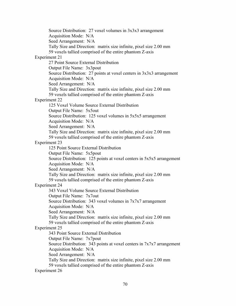
Source Distribution: 27 voxel volumes in 3x3x3 arrangement Acquisition Mode: N/A Seed Arrangement: N/A Tally Size and Direction: matrix size infinite, pixel size 2.00 mm 59 voxels tallied comprised of the entire phantom Z-axis
Experiment 21 27 Point Source External Distribution Output File Name: 3x3pout Source Distribution: 27 points at voxel centers in 3x3x3 arrangement Acquisition Mode: N/A Seed Arrangement: N/A Tally Size and Direction: matrix size infinite, pixel size 2.00 mm 59 voxels tallied comprised of the entire phantom Z-axis
Experiment 22 125 Voxel Volume Source External Distribution Output File Name: 5x5out Source Distribution: 125 voxel volumes in 5x5x5 arrangement Acquisition Mode: N/A Seed Arrangement: N/A Tally Size and Direction: matrix size infinite, pixel size 2.00 mm 59 voxels tallied comprised of the entire phantom Z-axis
Experiment 23 125 Point Source External Distribution Output File Name: 5x5pout Source Distribution: 125 points at voxel centers in 5x5x5 arrangement Acquisition Mode: N/A Seed Arrangement: N/A Tally Size and Direction: matrix size infinite, pixel size 2.00 mm 59 voxels tallied comprised of the entire phantom Z-axis
Experiment 24 343 Voxel Volume Source External Distribution Output File Name: 7x7out Source Distribution: 343 voxel volumes in 7x7x7 arrangement Acquisition Mode: N/A Seed Arrangement: N/A Tally Size and Direction: matrix size infinite, pixel size 2.00 mm 59 voxels tallied comprised of the entire phantom Z-axis
Experiment 25 343 Point Source External Distribution Output File Name: 7x7pout Source Distribution: 343 points at voxel centers in 7x7x7 arrangement Acquisition Mode: N/A Seed Arrangement: N/A Tally Size and Direction: matrix size infinite, pixel size 2.00 mm 59 voxels tallied comprised of the entire phantom Z-axis
Experiment 26
70
3375 Voxel Volume Source External Distribution Output File Name: 15vouz Source Distribution: 3375 voxel volumes in 15x15x15 arrangement Acquisition Mode: N/A Seed Arrangement: N/A Tally Size and Direction: matrix size infinite, pixel size 2.00 mm 59 voxels tallied comprised of the entire phantom Z-axis
Experiment 27 3375 Point Source External Distribution Output File Name: 15poux Source Distribution: 3375 points at voxel centers in 15x15x15 arrangement Acquisition Mode: N/A Seed Arrangement: N/A Tally Size and Direction: matrix size infinite, pixel size 2.00 mm 59 voxels tallied comprised of the entire phantom Z-axis
A.3 Energy Deposition Distributions From Second Scan Measured Data Experiment 28
Single Seed First Scan Set 128—5 slices Output File Name: rpt4ouv Source Distribution: PET/CT measured distribution of 5 pixel x 5 pixel x 5 slice Acquisition Mode: Two-dimensional Seed Arrangement One Tally Size and Direction: matrix size 128x128, pixel size 4.69 mm Positive X, 9 voxels, pixel size 4.69 mm Positive Z, 16 voxels, slice thickness 3.27 mm
Experiment 29 Single Seed First Scan Set 128—9 slices Output File Name: rpt5ouu Source Distribution: PET/CT measured distribution of 9 pixel x 9 pixel x 9 slice Acquisition Mode: Two-dimensional Seed Arrangement One Tally Size and Direction: matrix size 128x128, pixel size 4.69 mm Positive X, 9 voxels, pixel size 4.69 mm Positive Z, 16 voxels, slice thickness 3.27 mm
Experiment 30 Double Seed First Scan Set 128—5 slices Output File Name: rp2s3ouv Source Distribution: PET/CT measured distribution of 5 pixel x 5 pixel x 5 slice Acquisition Mode: Two-dimensional Seed Arrangement Two Tally Size and Direction: matrix size 128x128, pixel size 4.69 mm Negative X, 9 voxels, pixel size 4.69 mm Positive Z, 16 voxels, slice thickness 3.27 mm
Experiment 31
71
Double Seed First Scan Set 128—9 slices Output File Name: rp2s4ouu Source Distribution: PET/CT measured distribution of 9 pixel x 9 pixel x 9 slice Acquisition Mode: Two-dimensional Seed Arrangement Two Tally Size and Direction: matrix size 128x128, pixel size 4.69 mm Negative X, 9 voxels, pixel size 4.69 mm Positive Z, 16 voxels, slice thickness 3.27 mm
Experiment 32 Triple Seed First Scan Set 128—5 slices Output File Name: rp3s3ouz Source Distribution: PET/CT measured distribution of 5 pixel x 5 pixel x 5 slice Acquisition Mode: Two-dimensional Seed Arrangement Three Tally Size and Direction: matrix size 128x128, pixel size 4.69 mm Negative Y, 9 voxels, pixel size 4.69 mm Positive Z, 16 voxels, slice thickness 3.27 mm
Experiment 33 Triple Seed First Scan Set 128—9 slices Output File Name: rp3s4oux Source Distribution: PET/CT measured distribution of 9 pixel x 9 pixel x 9 slice Acquisition Mode: Two-dimensional Seed Arrangement Three Tally Size and Direction: matrix size 128x128, pixel size 4.69 mm Negative Y, 9 voxels, pixel size 4.69 mm Positive Z, 16 voxels, slice thickness 3.27 mm
Experiment 34 Single Seed First Scan Set 256—5 slices Output File Name: rpt7ouv Source Distribution: PET/CT measured distribution of 9 pixel x 9 pixel x 5 slice Acquisition Mode: Three-dimensional Seed Arrangement One Tally Size and Direction: matrix size 256x256, pixel size 2.34 mm Positive X, 18 voxels, pixel size 2.34 mm Positive Z, 16 voxels, slice thickness 3.27 mm
Experiment 35 Single Seed First Scan Set 256—9 slices Output File Name: rpt8ouz Source Distribution: PET/CT measured distribution of 17 pixel x 17 pixel x 9 slice Acquisition Mode: Three-dimensional Seed Arrangement One Tally Size and Direction: matrix size 256x256, pixel size 2.34 mm Positive X, 18 voxels, pixel size 2.34 mm Positive Z, 16 voxels, slice thickness 3.27 mm
Experiment 36
72

Double Seed First Scan Set 256—5 slices Output File Name: rp2s5ouu Source Distribution: PET/CT measured distribution of 9 pixel x 9 pixel x 5 slice Acquisition Mode: Three-dimensional Seed Arrangement Two Tally Size and Direction: matrix size 256x256, pixel size 2.34 mm Negative X, 18 voxels, pixel size 2.34 mm Positive Z, 16 voxels, slice thickness 3.27 mm
Experiment 37 Double Seed First Scan Set 256—9 slices Output File Name: rpts6ouu Source Distribution: PET/CT measured distribution of 17 pixel x 17 pixel x 9 slice Acquisition Mode: Three-dimensional Seed Arrangement Two Tally Size and Direction: matrix size 256x256, pixel size 2.34 mm Negative X, 18 voxels, pixel size 2.34 mm Positive Z, 16 voxels, slice thickness 3.27 mm
Experiment 38 Triple Seed First Scan Set 256—5 slices Output File Name: rp3s5ouv Source Distribution: PET/CT measured distribution of 9 pixel x 9 pixel x 5 slice Acquisition Mode: Three-dimensional Seed Arrangement Three Tally Size and Direction: matrix size 256x256, pixel size 2.34 mm Negative Y, 18 voxels, pixel size 2.34 mm Positive Z, 9 voxels, slice thickness 3.27 mm
Experiment 39 Triple Seed First Scan Set 256—9 slices Output File Name: rp3s6ouw Source Distribution: PET/CT measured distribution of 17 pixel x 17 pixel x 9 slice Acquisition Mode: Three-dimensional Seed Arrangement Three Tally Size and Direction: matrix size 256x256, pixel size 2.34 mm Negative Y, 18 voxels, pixel size 2.34 mm Positive Z, 9 voxels, slice thickness 3.27 mm
Experiment 40 Single Seed Second Scan Set (also Maximum Error Bound Voxel Center) Output File Name: meb1ouv Source Distribution: PET/CT measured distribution of 5 pixel x 5 pixel x 5 slice Acquisition Mode: Two-dimensional Seed Arrangement One Tally Size and Direction: matrix size 128x128, pixel size 4.69 mm Positive X, 9 voxels, pixel size 4.69 mm Positive Z, 16 voxels, slice thickness 3.27 mm
73

Experiment 41 Single Seed Second Scan Set 256 (also Maximum Error Bound Voxel Center) Output File Name: meb4ouu Source Distribution: PET/CT measured distribution of 9 pixel x 9 pixel x 5 slice Acquisition Mode: Two-dimensional Seed Arrangement One Tally Size and Direction: matrix size 256x256, pixel size 2.34 mm Positive X, 18 voxels, pixel size 2.34 mm Positive Z, 16 voxels, slice thickness 3.27 mm
Experiment 42 Maximum Error Bound Negative X Shift 128 Output File Name: meb2ouy Source Distribution: PET/CT measured distribution Acquisition Mode: Two-dimensional Seed Arrangement One Tally Size and Direction: matrix size 128x128, pixel size 4.69 mm Positive X, 9 voxels, pixel size 4.69 mm
Experiment 43 Maximum Error Bound Positive X Shift 128 Output File Name: meb3ouy Source Distribution: PET/CT measured distribution Acquisition Mode: Two-dimensional Seed Arrangement One Tally Size and Direction: matrix size 128x128, pixel size 4.69 mm Positive X, 9 voxels, pixel size 4.69 mm
Experiment 44 Maximum Error Bound Negative X Shift 256 Output File Name: meb5ouv Source Distribution: PET/CT measured distribution Acquisition Mode: Three-dimensional Seed Arrangement One Tally Size and Direction: matrix size 256x256, pixel size 2.34 mm Positive X, 18 voxels, pixel size 2.34 mm
Experiment 45 Maximum Error Bound Positive X Shift 256 Output File Name: meb6ouu Source Distribution: PET/CT measured distribution Acquisition Mode: Three-dimensional Seed Arrangement One Tally Size and Direction: matrix size 256x256, pixel size 2.34 mm Positive X, 18 voxels, pixel size 2.34 mm
Experiment 46 Triple Seed Second Scan Set Output File Name: 3sa3ouu Source Distribution: PET/CT measured distribution of 5 pixel x 5 pixel x 5 slice Acquisition Mode: Two-dimensional
74
Seed Arrangement Three Tally Size and Direction: matrix size 128x128, pixel size 4.69 mm Negative X, 9 voxels, pixel size 4.69 mm Positive Z, 16 voxels, slice thickness 3.27 mm
Experiment 47 Triple Seed Second Scan Set Output File Name: 3sa4out Source Distribution: PET/CT measured distribution of 9 pixel x 9 pixel x 5 slice Acquisition Mode: Two-dimensional Seed Arrangement Three Tally Size and Direction: matrix size 256x256, pixel size 2.34 mm Negative X, 18 voxels, pixel size 2.34 mm Positive Z, 16 voxels, slice thickness 3.27 mm
Experiment 48 Single Seed Second Scan Set Brain Protocol 128 Output File Name: branouu Source Distribution: PET/CT measured distribution of 5 pixel x 5 pixel x 5 slice Acquisition Mode: Two-dimensional Seed Arrangement One Tally Size and Direction: matrix size 128x128, pixel size 4.69 mm Positive X, 9 voxels, pixel size 4.69 mm Positive Z, 16 voxels, slice thickness 3.27 mm
Experiment 49 Single Seed Second Scan Set Brain Protocol 256 Output File Name: brn2ouw Source Distribution: PET/CT measured distribution of 18 pixel x 18 pixel x 5 slice Acquisition Mode: Two-dimensional Seed Arrangement One Tally Size and Direction: matrix size 256x256, pixel size 1.17 mm Positive X, 37 voxels, pixel size 1.17 mm Positive Z, 16 voxels, slice thickness 3.27 mm
75

APPENDIX B
GRAPHS AND TABLES OF COMPUTATIONAL RESULTS
This appendix contains graphs comparing energy deposition per voxel.
The tables below have additional calculations as follows:
Relative Discrepancy
Source Ideal From DepositedEnergy
Data Measured From DepositedEnergy =
DepositionEnergy Center DepositionEnergy ShiftedBoundError Actual =
( ) ( ) ( )22 Error RelativeCenter Error Relative ShiftedBoundError Actual BoundError Absolute +=
MCNP Calculated Energy DepositionBased on 2-D Acquisition of One Seed
Positive Z-Axis Comparison
1.00E-06
1.00E-05
1.00E-04
1.00E-0316 15 14 13 12 11 10 9 8 7 6 5 4 3 2 1
Voxel Distance From Origin (3.27mm)
Ener
gy D
epos
ition
(M
eV)
Theor etical
5x5x5 Sl ice
9x9x9 Sl ice
Figure 18. Transaxial energy deposition for the one seed case for theoretical versus PET measured source distributions. The PET data were acquired with 128x128 matrix, 3.27 mm slice thickness, 2D acquisition mode and OSEM reconstruction.
76

MCNP Calculated Energy DepositionBased on 3-D Acquisition of One Seed
Positive Z-Axis Comparison
1.00E-07
1.00E-06
1.00E-05
1.00E-04
1.00E-0316 15 14 13 12 11 10 9 8 7 6 5 4 3 2 1
Voxel Distance From Origin (3.27 mm)
Ener
gy D
epos
ition
(M
eV)
Theoret ical
9x9x5 Slice
17x17x9 Slice
Figure 19. Transaxial energy deposition for one seed case for theoretical versus PET measured source distributions. The PET data were acquired with 256 x 256 matrix, 3.27 mm slice thickness, 3D acquisition mode and 3D FORE IR reconstruction.
MCNP Calculated Energy DepositionBased on 2-D Acquisition of Two Seeds
Positive Z-Axis Comparison
1.00E-06
1.00E-05
1.00E-04
1.00E-0316 15 14 13 12 11 10 9 8 7 6 5 4 3 2 1
Voxel Distance From Origin (3.27mm)
Ener
gy D
epos
ition
(MeV
)
Theoretical
5x5x5 Slice
9x9x9 Slice
Figure 20. Transaxial energy deposition for the two seed case for theoretical versus PET measured source distributions. The PET data were acquired with 128x128 matrix, 3.27 mm slice thickness, 2D acquisition mode and OSEM reconstruction.
77

MCNP Calculated Energy DepositionBased on 3-D Acquisition of Two Seeds
Negative X-Axis Comparison
1.00E-06
1.00E-05
1.00E-04
1.00E-0318 17 16 15 14 13 12 11 10 9 8 7 6 5 4 3 2 1
Voxel Distance From Origin (2.34 mm)
Ener
gy D
epos
ition
(MeV
)
Theoretical
9x9x5 Slice
17x17x9 Slice
Figure 21. Transaxial energy deposition for two seed case for theoretical versus PET measured source distributions. The PET data were acquired with 256 x 256 matrix, 2.34 mm pixel size, 3D acquisition mode and 3D FORE IR reconstruction.
MCNP Calculated Energy DepositionBased on 3-D Acquisition of Two Seeds
Positive Z-Axis Comparison
1.00E-07
1.00E-06
1.00E-05
1.00E-04
1.00E-0316 15 14 13 12 11 10 9 8 7 6 5 4 3 2 1
Voxel Distance From Origin (3.27 mm)
Ener
gy D
epos
ition
(MeV
)
Theoretical
9x9x5 Slice
17x17x9 Slice
Figure 22. Transaxial energy deposition for two seed case for theoretical versus PET measured source distributions. The PET data were acquired with 256 x 256 matrix, 3.27 mm slice thickness, 3D acquisition mode and 3D FORE IR reconstruction.
78
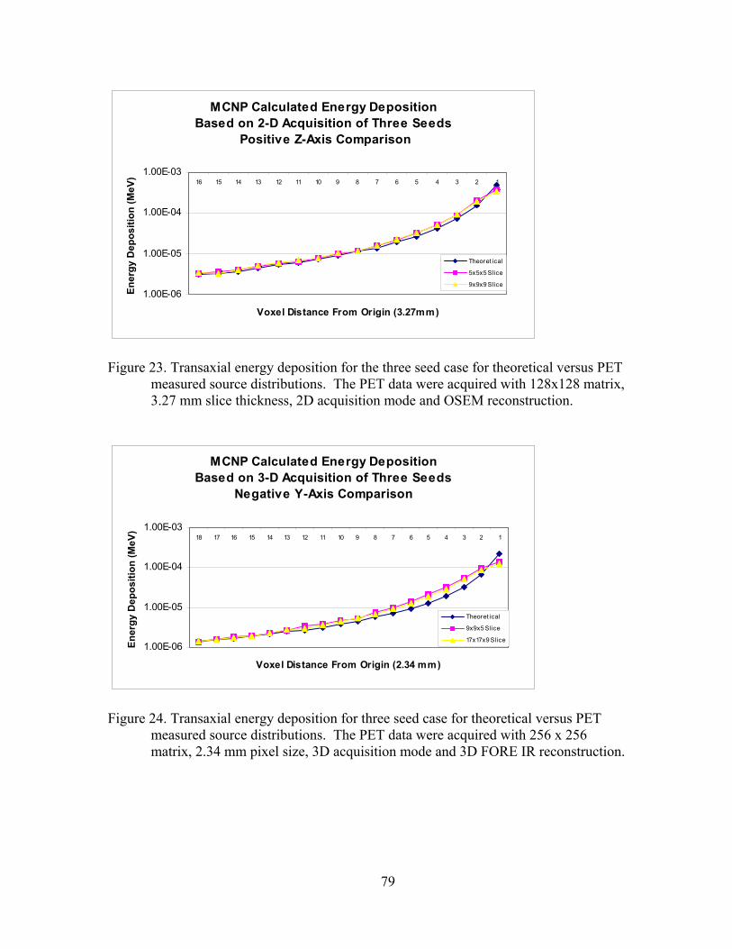
MCNP Calculated Energy DepositionBased on 2-D Acquisition of Three Seeds
Positive Z-Axis Comparison
1.00E-06
1.00E-05
1.00E-04
1.00E-0316 15 14 13 12 11 10 9 8 7 6 5 4 3 2 1
Voxel Distance From Origin (3.27mm)
Ener
gy D
epos
ition
(MeV
)
Theoret ical
5x5x5 Slice
9x9x9 Slice
Figure 23. Transaxial energy deposition for the three seed case for theoretical versus PET measured source distributions. The PET data were acquired with 128x128 matrix, 3.27 mm slice thickness, 2D acquisition mode and OSEM reconstruction.
MCNP Calculated Energy DepositionBased on 3-D Acquisition of Three Seeds
Negative Y-Axis Comparison
1.00E-06
1.00E-05
1.00E-04
1.00E-0318 17 16 15 14 13 12 11 10 9 8 7 6 5 4 3 2 1
Voxel Distance From Origin (2.34 mm)
Ener
gy D
epos
ition
(MeV
)
Theoret ical
9x9x5 Slice
17x17x9 Slice
Figure 24. Transaxial energy deposition for three seed case for theoretical versus PET measured source distributions. The PET data were acquired with 256 x 256 matrix, 2.34 mm pixel size, 3D acquisition mode and 3D FORE IR reconstruction.
79
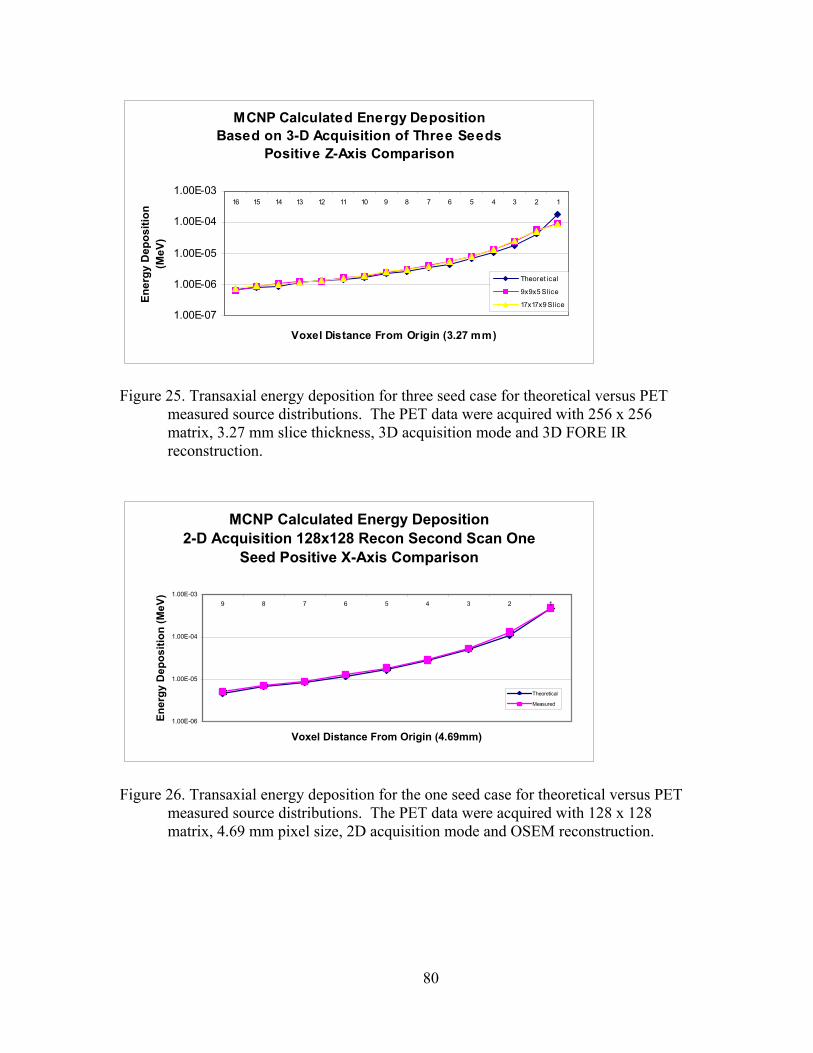
MCNP Calculated Energy DepositionBased on 3-D Acquisition of Three Seeds
Positive Z-Axis Comparison
1.00E-07
1.00E-06
1.00E-05
1.00E-04
1.00E-0316 15 14 13 12 11 10 9 8 7 6 5 4 3 2 1
Voxel Distance From Origin (3.27 mm)
Ener
gy D
epos
ition
(M
eV)
Theoret ical
9x9x5 Slice
17x17x9 Slice
Figure 25. Transaxial energy deposition for three seed case for theoretical versus PET measured source distributions. The PET data were acquired with 256 x 256 matrix, 3.27 mm slice thickness, 3D acquisition mode and 3D FORE IR reconstruction.
MCNP Calculated Energy Deposition2-D Acquisition 128x128 Recon Second Scan One
Seed Positive X-Axis Comparison
1.00E-06
1.00E-05
1.00E-04
1.00E-039 8 7 6 5 4 3 2 1
Voxel Distance From Origin (4.69mm)
Ener
gy D
epos
ition
(MeV
)
Theoretical
Measured
Figure 26. Transaxial energy deposition for the one seed case for theoretical versus PET measured source distributions. The PET data were acquired with 128 x 128 matrix, 4.69 mm pixel size, 2D acquisition mode and OSEM reconstruction.
80

MCNP Calculated Energy Deposition2-D Acquisition 256x256 Recon Second Scan
One Seed Positive X-Axis Comparison
1.00E-06
1.00E-05
1.00E-04
1.00E-0318 17 16 15 14 13 12 11 10 9 8 7 6 5 4 3 2 1
Voxel Distance From Origin (2.34mm)
Ener
gy D
epos
ition
(MeV
)
Theoretical
Measured
Figure 27. Transaxial energy deposition for the one seed case for theoretical versus PET measured source distributions. The PET data were acquired with 256 x 256 matrix, 2.34 mm pixel size, 2D acquisition mode and OSEM reconstruction.
MCNP Calculated Energy Deposition2-D Acquisition 128x128 Recon Second Scan
One Seed Positive Z-Axis Comparison
1.00E-06
1.00E-05
1.00E-04
1.00E-0316 15 14 13 12 11 10 9 8 7 6 5 4 3 2 1
Voxel Distance From Origin (3.27mm)
Ener
gy D
epos
ition
(MeV
)
Theoreticall
Measured
Figure 28. Transaxial energy deposition for the one seed case for theoretical versus PET measured source distributions. The PET data were acquired with 128x128 matrix, 3.27 mm slice thickness, 2D acquisition mode and OSEM reconstruction.
81
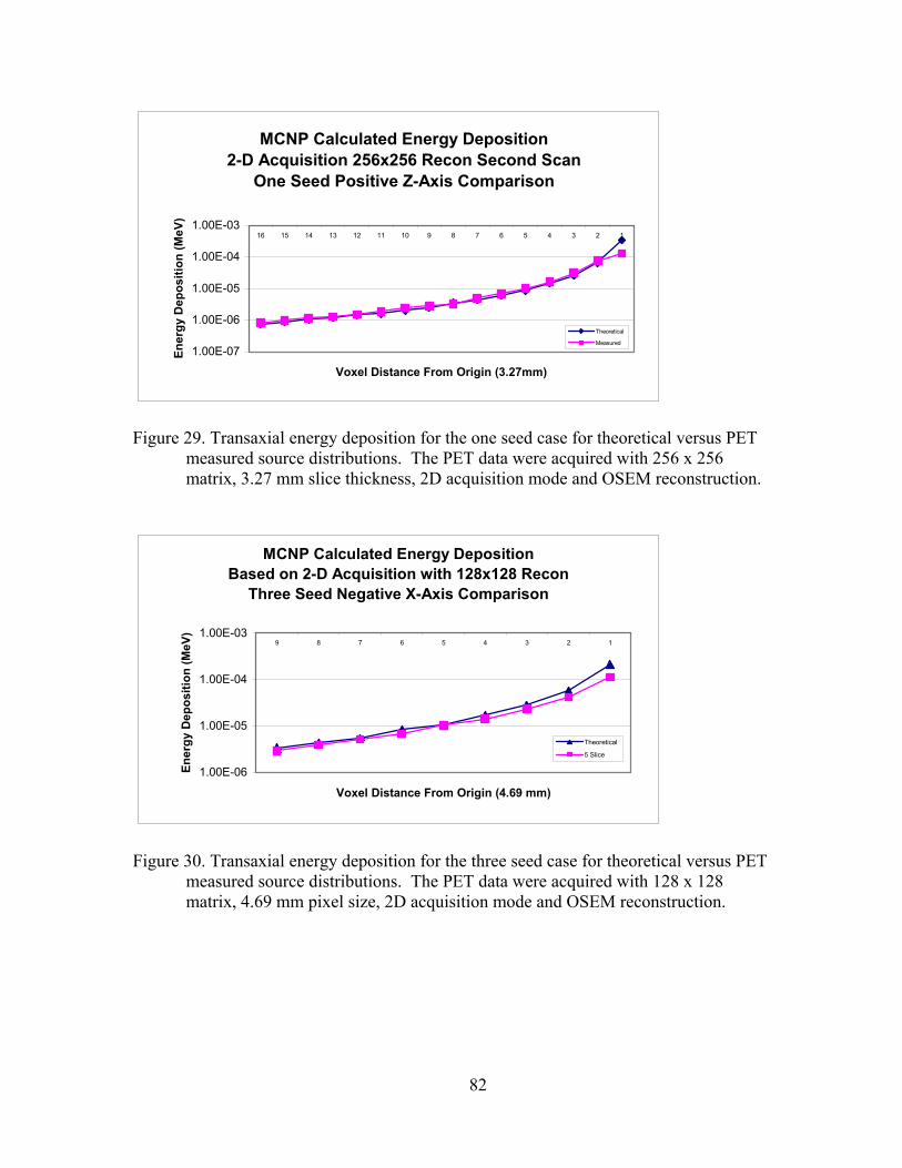
MCNP Calculated Energy Deposition2-D Acquisition 256x256 Recon Second Scan
One Seed Positive Z-Axis Comparison
1.00E-07
1.00E-06
1.00E-05
1.00E-04
1.00E-0316 15 14 13 12 11 10 9 8 7 6 5 4 3 2 1
Voxel Distance From Origin (3.27mm)
Ener
gy D
epos
ition
(MeV
)
Theoretical
Measured
Figure 29. Transaxial energy deposition for the one seed case for theoretical versus PET measured source distributions. The PET data were acquired with 256 x 256 matrix, 3.27 mm slice thickness, 2D acquisition mode and OSEM reconstruction.
MCNP Calculated Energy DepositionBased on 2-D Acquisition with 128x128 Recon
Three Seed Negative X-Axis Comparison
1.00E-06
1.00E-05
1.00E-04
1.00E-039 8 7 6 5 4 3 2 1
Voxel Distance From Origin (4.69 mm)
Ener
gy D
epos
ition
(MeV
)
Theoretical
5 Slice
Figure 30. Transaxial energy deposition for the three seed case for theoretical versus PET measured source distributions. The PET data were acquired with 128 x 128 matrix, 4.69 mm pixel size, 2D acquisition mode and OSEM reconstruction.
82

MCNP Calculated Energy DepositionBased on 2-D Acquisition With 256x256 Recon
Three Seed Negative X-Axis Comparison
1.00E-07
1.00E-06
1.00E-05
1.00E-04
1.00E-0318 16 14 12 10 8 6 4 2
Voxel Distance From Origin (2.34 mm)
Ener
gy D
epos
ition
(MeV
)
Theoretical
5 Slice
Figure 31. Transaxial energy deposition for the three seed case for theoretical versus PET measured source distributions. The PET data were acquired with 256 x 256 matrix, 2.34 mm pixel size, 2D acquisition mode and OSEM reconstruction.
MCNP Calculated Energy DepositionBased on 2-D Acquisition with 128x128 Recon
Three Seed Positive-Z Axis Comparison
1.00E-06
1.00E-05
1.00E-04
1.00E-0316 14 12 10 8 6 4 2
Voxel Distance From Origin (4.69 mm)
Ener
gy D
epos
ition
(MeV
)
Theoretical
5 Slice
Figure 32. Transaxial energy deposition for the three seed case for theoretical versus PET measured source distributions. The PET data were acquired with 128x128 matrix, 3.27 mm slice thickness, 2D acquisition mode and OSEM reconstruction.
83
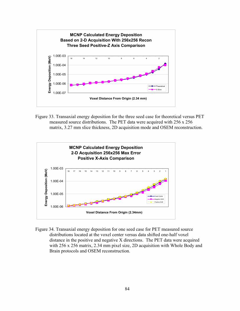
MCNP Calculated Energy DepositionBased on 2-D Acquisition With 256x256 Recon
Three Seed Positive-Z Axis Comparison
1.00E-07
1.00E-06
1.00E-05
1.00E-04
1.00E-0316 14 12 10 8 6 4 2
Voxel Distance From Origin (2.34 mm)
Ener
gy D
epos
ition
(MeV
)
Theoretical
5 Slice
Figure 33. Transaxial energy deposition for the three seed case for theoretical versus PET measured source distributions. The PET data were acquired with 256 x 256 matrix, 3.27 mm slice thickness, 2D acquisition mode and OSEM reconstruction.
MCNP Calculated Energy Deposition2-D Acquisition 256x256 Max Error
Positive X-Axis Comparison
1.00E-06
1.00E-05
1.00E-04
1.00E-0318 17 16 15 14 13 12 11 10 9 8 7 6 5 4 3 2 1
Voxel Distance From Origin (2.34mm)
Ener
gy D
epos
ition
(MeV
)
Voxel Center
Negative Shift
Positive Shift
Figure 34. Transaxial energy deposition for one seed case for PET measured source distributions located at the voxel center versus data shifted one-half voxel distance in the positive and negative X directions. The PET data were acquired with 256 x 256 matrix, 2.34 mm pixel size, 2D acquisition with Whole Body and Brain protocols and OSEM reconstruction.
84

MCNP Calculated Energy Deposition2-D Acquisition 128x128 Recon Second Scan
One Seed Positive Z-Axis Comparison
1.00E-06
1.00E-05
1.00E-04
1.00E-0316 15 14 13 12 11 10 9 8 7 6 5 4 3 2 1
Voxel Distance From Origin (3.27mm)
Ener
gy D
epos
ition
(MeV
)
Theoretical
Whole Body
Brain
Figure 35. Transaxial energy deposition for one seed case for theoretical versus PET
measured source distributions. The PET data were acquired with 128 x 128 matrix, 3.27 slice thickness, 2D acquisition with Whole Body and Brain protocols and OSEM reconstruction.
Brain Acquisition Protocol2-D Acquisition 256x256 Recon Second Scan
One Seed Positive X-Axis Comparison
1.00E-07
1.00E-06
1.00E-05
1.00E-04
1.00E-0337 34 31 28 25 22 19 16 13 10 7 4 1
Voxel Distance From Origin (1.17mm)
Ener
gy D
epos
ition
(MeV
)
Theoretical
Measured
Figure 36. Transaxial energy deposition for one seed case for theoretical versus PET measured source distributions. The PET data were acquired with 256 x 256 matrix, 1.17 mm pixel size, 2D acquisition with Brain protocol and OSEM reconstruction.
85

Brain Acquisition Protocol2-D Acquisition 256x256 Recon Second Scan
One Seed Positive Z-Axis Comparison
1.00E-07
1.00E-06
1.00E-05
1.00E-04
1.00E-0316 15 14 13 12 11 10 9 8 7 6 5 4 3 2 1
Voxel Distance From Origin (3.27mm)
Ener
gy D
epos
ition
(MeV
)
Theoretical
Measured
Figure 37. Transaxial energy deposition for one seed case for theoretical versus PET measured source distributions. The PET data were acquired with 256 x 256 matrix, 3.27 mm slice thickness, 2D acquisition with Brain protocol and OSEM reconstruction.
Z Axis Comparison 3x3x3
1.90E-04
2.00E-04
2.10E-04
2.20E-04
2.30E-04
2.40E-04
0 0 -1 0 0 0 0 0 1
Cell (2mm voxel size)
Ener
gy D
epos
ition
(MeV
)
Volume
Point
Figure 38. Point versus voxel volume source comparison of dose deposition inside a 3 x 3 x 3 source array arrangement.
86

Z Axis Comparison 5x5x5
6.00E-05
6.50E-05
7.00E-05
7.50E-05
8.00E-05
8.50E-05
9.00E-05
0 0 -2 0 0 -1 0 0 0 0 0 1 0 0 2
Cell (2mm voxel size)
Ener
gy D
epos
ition
(MeV
)
Volume
Point
Figure 39. Point versus voxel volume source comparison of dose deposition inside a 5 x 5 x 5 source array arrangement.
Z Axis Comparison 7x7x7
3.00E-053.20E-053.40E-053.60E-053.80E-054.00E-054.20E-054.40E-054.60E-05
0 0 -3 0 0 -2 0 0 -1 0 0 0 0 0 1 0 0 2 0 0 3
Cell (2mm voxel size)
Ener
gy D
epos
ition
(MeV
)
Volume
Point
Figure 40. Point versus voxel volume source comparison of dose deposition inside a 7 x 7 x 7 source array arrangement.
87

MCNP Calculated Energy DepositionSingle Point versus Single Voxel Source
Z-axis Comparison
1.00E-07
1.00E-06
1.00E-05
1.00E-04
1.00E-03
1.00E-0229 25 21 17 13 9 5 1 -3 -7 -11 -15 -19 -23 -27
Voxel Distance from Origin (2mm)
Ener
gy D
epos
ition
(MeV
)
Volume
Point
Figure 41. Point versus voxel volume source comparison of dose deposition for entire phantom using 1 voxel and 1 point arrangement.
MCNP Calculated Energy Deposition 3x3x3 Point versus 3x3x3 Voxel Source
Z-axis Comparison
1.00E-07
1.00E-06
1.00E-05
1.00E-04
1.00E-0329 25 21 17 13 9 5 1 -3 -7 -11 -15 -19 -23 -27
Voxel Distance from Origin (2mm)
Ener
gy D
epos
ition
(Mev
)
Volume
Point
Figure 42. Point versus voxel volume source comparison of dose for entire phantom using 3 x 3 x 3 arrangement.
88

MCNP Calculated Energy Deposition5x5x5 Point versus 5x5x5 Voxel Source
Z-axis Comparison
1.00E-07
1.00E-06
1.00E-05
1.00E-0429 25 21 17 13 9 5 1 -3 -7 -11 -15 -19 -23 -27
Voxel Distance from Origin (2mm)
Ener
gy D
epos
ition
(MeV
)
Volume
Point
Figure 43. Point versus voxel volume source comparison of dose for entire phantom using 5 x 5 x 5 arrangement.
MCNP Calculated Energy Deposition7x7x7 Point versus 7x7x7 Voxel Source
Z-axis Comparison
1.00E-07
1.00E-06
1.00E-05
1.00E-0429 25 21 17 13 9 5 1 -3 -7 -11 -15 -19 -23 -27
Voxel Distance from Origin (2mm)
Ener
gy D
epos
ition
(MeV
)
Volume
Point
Figure 44. Point versus voxel volume source comparison of dose for entire phantom using 7 x 7 x 7 arrangement.
89

Table 7. Values plotted in Figure 9 and Figure 18 with associated MCNP error and relative discrepancy.
90

Table 8. Values plotted in Figure 12 and Figure 19 with associated MCNP error and relative discrepancy.
91

Table 9. Values plotted in Figure 10 and Figure 20 with associated MCNP error and relative discrepancy.
92

Table 10. Values plotted in Figure 21 and Figure 22 with associated MCNP error and relative discrepancy.
93

Table 11. Values plotted in Figure 11 and Figure 23 with associated MCNP error and relative discrepancy.
94

Table 12. Values plotted in Figure 24 and Figure 25 with associated MCNP error and relative discrepancy.
95

Table 13. Values plotted in Figure 26 and Figure 28 with associated MCNP error and relative discrepancy.
96

Table 14. Values plotted in Figure 27 and Figure 29 with associated MCNP error and relative discrepancy.
97

Table 15. Values plotted in Figure 30 and Figure 32 with associated MCNP error and relative discrepancy.
98

Table 16. Values plotted in Figure 31 and Figure 33 with associated MCNP error and relative discrepancy.
99

Table 17. Values plotted in Figure 14 with associated MCNP error and actual and absolute error bounds.
Table 18. Values plotted in Figure 34 with associated MCNP error and actual and absolute error bounds.
100

Table 19. Values plotted in Figure 13 and Figure 35 with associated MCNP error and relative discrepancy.
101

APPENDIX C
IDL DATA EXTRACTION PROGRAM FOR DICOM
This is a copy of the IDL program utilized for extraction and scaling of the PET
data located in DICOM format files:
;This IDL program extracts the raw DICOM data ;by extracting the stored pixel value and then ;multiplying the entire array by the scaling ;factor pro mikesthesis3 ;This loop cycles through multiple slices ;FOR i=847,801,-1 DO BEGIN i=729 ;this line is for processing a single slice j=string(i) k=STRCOMPRESS(strtrim(j,2)) correctfile ='D:\1seed256brain\'+k obj = OBJ_NEW('IDLffDICOM') read = obj->Read(correctfile) ; Get the image data ;array is the actual raw number array = obj->GetValue('7fe0'x, '0010'x) ;scaled is the slice scaling factor scaled = obj->GetValue('0028'x, '1053'x) ;slice is the slice number slice = obj->GetValue('0020'x, '0013'x) ;scaledvalue and slicenumber truncates spaces scaledvalue = double(*scaled[0]) slicenumber = fix(*slice[0]) OBJ_DESTROY, obj ;MikesArray is the array of the pixel ;value multiplied by the scaling factor MikesArray = (*array[0])*scaledvalue ; Open a new file for writing as IDL file unit number 1: OPENU, 1, 'RawData.txt',/append OPENU, 2, 'SliceScale.txt',/append ; Write the data to the file: PRINTF, 1, mikesarray PRINTF, 2, slicenumber, scaledvalue ; Close file unit 1: CLOSE, 1 CLOSE, 2 TVScl, mikesarray PTR_FREE, array ;ENDFOR
end
102
APPENDIX D
MCNP5 TUTORIAL
A brief summary of the most relevant MCNP input parameters are summarized
for the reader interested in perusing the actual MCNP input files of this study.[62, 63]
The input for MCNP5 follows a specific syntax and structure. First the geometry is
specified by cell definitions followed by the surfaces that define them. Following next is
the mode of operation, relative importance of each cell, and the source definition. Then
the type of result or tallies is specified. Next is the material description. Finally, the
number of histories and other output parameters are specified.
All space must be accounted for in cell definition. The Visual Editor (VisEd)
version 12N, released in November of 2002, allows the user to set up and modify the
view of the MCNP geometry so that immediate feedback is available of input
adjustments. VisEd can display surface and cell numbers with different materials
represented by different colors. Views are in 2D and the basis may be changed to any of
the possible combinations x-y, x-z, y-x, y-z, z-x, z-y while also facilitating zooming in or
out as well as moving the origin in any of three directions to obtain the desired
perspective. Cells may be defined with a variety of surfaces and geometries. MCNP
utilizes the Cartesian coordinate system for geometric cell definition. The cell number,
material number, and material density define each cell on the cell card. Next follows a
combination of surfaces that form the cell boundary. Planes, cylinders, spheres, cones,
and other surfaces are described in the MCNP5 manual. The input file is generally
referred to as a deck consisting of four cards in the format as follows:
One-line Problem Title Card
103

Cell Cards
…
…
Blank Line Delimiter
Surface Cards
…
…
Blank Line Delimiter
Data Cards
…
…
All input lines are limited to 80 columns. Comment cards can be used anywhere
in the input file by either placing a C in columns 1-5 followed by at least one blank and
can be a total of 80 columns long, or can be appended to an existing input line by the $
operator followed by a space and the comment to follow. Cell, surface and data cards
must begin within the first five columns. MCNP executes extensive input file checks for
user errors, but is not foolproof.
The cell card structure starts with the cell number in the first five columns. The
next entry is the cell material number defined by the user in the data card. Next is the cell
material density with a positive entry interpreted as atom density in units of 1024
atoms/cm3 while a negative entry is interpreted as mass density in g/cm3. A complete
specification of the cell geometry follows. Cell geometry can be defined with
intersection, union, or compliment of surfaces. The exclusion operator is used to exclude
104

a cell from the cell being defined with the number sign (#) followed by the excluded cell.
Optionally, cell parameters can be entered with the form keyword = value. Some
parameters might be importance, universe, fill, or lattice. Repeated structure and lattice
elements are advanced features of MCNP geometry formats utilized for this project.
For the cell description describing all space below the plane z = 3, the cell card
for cell one of material one, adult tissue, would be as follows:
1 1 -1.04 -1 $cell one, tissue material number, tissue density, surface
For the surface card, the first entry is the surface number that must be in column
1-5 and not exceed 5 digits. The next entry is an alphabetic mnemonic indicating the
surface type followed by numerical coefficients of the surface equation in specified order.
Each surface divides space with a positive and negative sense indicated by the sign of the
surface in the cell card. For example, for a plane surface number one normal to the z-axis
at z = 3 are defined as follows in the surface card:
1 pz 3 $surface one, plane normal to z axis at z = 3
The data cards form the remaining data input. The card name is the first entry and
must begin in the first five columns. The required entries are:
Entry MCNP card name
mode, MODE
cell and surface parameters, IMP:P
source specification, SDEF
tally specification, Fn, En
material specification, Mn
problem cutoffs, NPS
105
The source specification is generally the most difficult part of input to arrange.
Source specification allows photon, neutron, or electron type in a variety of energies,
locations, distributions, and probabilities. The MODE card consists of the mnemonic
MODE followed by the choice of particle such as MODE p e for photon and electron
transport. Cell and surface parameter cards define values of cell parameters. One
example used by this study is the importance card that specifies the relative cell
importance where the number of entries on the parameter card must equal the number of
cells in the problem. Multiple entries may be entered using the entry followed by a
number of repeats and the letter r. For example, a photon importance of 1 for 100 cells
may be written as imp:p 1 99r. The source specification card, SDEF, defines the basic
source parameters. Some of these basic source input parameters include position (POS),
starting cell (CEL), starting energy (ERG), starting weight (WGT), source particle type
(PAR). These may be included in the SDEF card in any order and the equals sign is not
needed for assigning parameter value. Source definitions can be points, distributions
within a volume, or spectrums defined by further dependence. Source variables may
depend on other variables and can quickly become quite complex in nature.
The tally cards specify what information you want from the Monte Carlo
calculation. Various tallies related to transport are requested with MCNP5 such as
particle current, particle flux, and energy deposition. Many of the tally specification
“bins” are for example energy (En), time (Tn), and cosine (Cn). MCNP provides six
standard neutron, six standard photon, and four standard electron tallies, all normalized to
be per starting particle. In addition to tally information, the output file contains tables of
summary information for information on the calculation run. Print table 110 was used to
106

verify source specification by identifying the starting location and direction of the first
fifty histories. The final table indicates important statistical checks such as the mean,
error, the variance of variance (VOV), the slope or the largest history scores fluctuate as a
function of the number of histories run, and the figure of merit (FOM). Printed with each
tally is its statistical relative error corresponding to the fraction of one standard deviation.
MCNP tallies are normalized to one particle. Even though MCNP is highly regarded and
experimentally verified, these confidence statements refer to the precision of the Monte
Carlo calculation itself and not to the accuracy of the result compared to true physical
values.
The material cards specify both isotropic composition of the materials and the
cross-section evaluations for the designated cells. The format of the material (Mm) card
for material 3 as water (H2O) is given as an example:
C Water (Density = 1.00 g/cc)
M3 1000 -0.111894 $ Hydrogen fraction
8000 -0.888106 $ Oxygen fraction
Problem cutoff cards are used for some of the ways to terminate execution of
MCNP. For our problems the history cutoff (NPS) card is used.
Uncertainty is as important as the MCNP answer itself. The history score
probability density function, f(x), where x is the tally estimate, is seldom known therefore
the true mean is estimated by the sample mean. The estimated relative error (R) can be
used to form confidence intervals about the estimated mean, allowing one to make a
statement about what the true result is. For a well-behaved tally Equation D.1 shows the
relationship between R and N, the number of histories.
107

NR 1
∝ (D.1)
Thus, to halve R, we must increase N, the total number of histories, fourfold.
MCNP recommends R < 0.10 however enough histories were calculated so the results
have a one sigma value less than 0.02, if possible, within 5 cm.[5] We almost always
obtained R < 0.05 which is considered generally reliable for point detectors, and point
detectors require more precision than the much larger voxel volume tallies we used so the
R we achieved should be more than adequate. The relative error is a convenient number
because it represents statistical precision as a fractional result with respect to the
estimated mean. The other two desired behaviors of the relative error are that it is
decreasing and has a decreasing rate of decrease as a function of NPS.
The VOV is the estimate of the error of the relative error and it checks the tally
history scores for any effects of inadequately sampled problems. It can detect tally errors
due to insufficient sampling of high weight scores that can cause underestimated mean
and relative error. VOV is the estimated relative variance of the estimated R. It should
be below 0.10 to improve the probability of forming a reliable confidence interval, but
the lower the better. The other two desired behaviors of the variance of the variance are
that it is decreasing and has a decreasing rate as a function of NPS.
The more efficient a Monte Carlo calculation is, the larger the FOM will be
because less computer time is required to reach a given R. Equation D.2 relates the FOM
to R and T, computational time.
TRFOM
2
1= (D.2)
108
The FOM can be a reliable indicator if the tally is well behaved. It should be
roughly constant and random in behavior. Rapid large changes in FOM indicate
sampling problems that need attention. For instance, a sharp decrease in FOM indicates a
seldom-sampled particle path has significantly affected the tally result and relative error
estimate.
The slope refers to the history score with the estimated exponent of the
probability density function’s large score behavior. The slope is defined by Equation D.3
where the k value is found by the robust “simplex” algorithm[66] that best fit the largest
history scores by maximum likelihood estimation.
+≡ 11
kSlope (D.3)
The maximum slope score is a perfect 10 and zero means not enough information was
available for the calculation. A slope above 3 is desired to satisfy the second moment
existence requirement of the Central Limit Theorem (CLT). The CLT states that the
estimated mean will appear to be sampled from a normal distribution with a known
standard deviation. When N approaches infinity there is a 68% chance that the true result
is in the range of one R from the mean and a 95% chance that the answer is within 2 R’s
of the mean. As the slope increases, a more reliable confidence interval is formed
because the tally PDF appears to be more completely sampled.
It is extremely important to note that these confidence statements refer only to the
precision of the Monte Carlo calculation itself and not to the accuracy of the result
compared to the true physical value. In all runs, all statistical checks were verified.
109

APPENDIX E
DICOM STANDARD
The Digital Imaging and Communications in Medicine (DICOM) standard is a
2113 page sixteen-part document published by the National Electrical Manufacturers
Association (NEMA) to provide a standard method for transferring images and associated
information between devices manufactured by various vendors.[61] In practice, DICOM
aids in the distribution and viewing of different types of medical images such as CT,
ultrasound, MRI, and PET. A full download copy of the standard is available online at
http://medical.nema.org/medical/Dicom/ with drafts organized by year. The standard
describes a file format for the distribution of images that is an extension of an older
NEMA standard. Most people refer to image files that are compliant with the DICOM
standard as DICOM format files.
A DICOM file consists of the image data preceded by a header that stores detailed
information about the scan and images. DICOM requires a 128-byte preamble that is
usually all set to zero followed by the letters 'D', 'I', 'C', 'M'. This is followed by the
details of the header information described by tags with two four-digit hexadecimal
numbers in the form (gggg,eeee). The first number is the group number; the second
number is the element number. The DICOM header group and element components that
are required for certain image types are listed in Part 3 of the standard. For example,
image modality 'PT' found in group,element (0008,0060) should have elements to
describe the PET radiopharmaceutical or it would be in violation of the DICOM standard.
Of particular importance is group,element (0002,0010) that defines the Transfer Syntax
Unique Identification. This value reports the structure of the image data, revealing
110

whether the data has been compressed. It has a direct influence on how the Pixel Data
Element (7FE0,0010) shall be used for the exchange of encoded graphical image
data.[61]
For viewing purposes, image data is stored as pixel values with the largest raw
output value for each slice scaled to the maximum unsigned two-byte integer value of
32,767. DICOM provides different formats for scaling slice data, but all images analyzed
in this study used direct linear scaling. This linear scaling is in line equation format of
y=mx+b where y is the raw output value, x is the pixel value, m is the scaling factor, and
b is the data shift value that is zero for all study images.
111
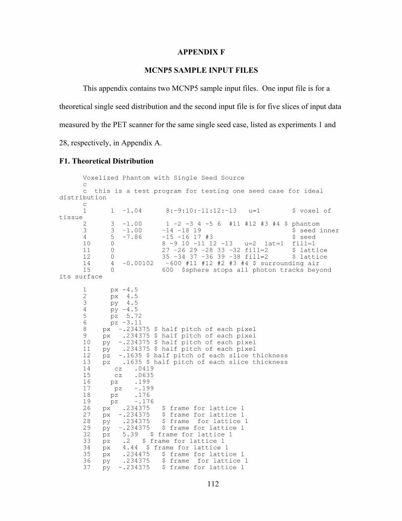
APPENDIX F
MCNP5 SAMPLE INPUT FILES
This appendix contains two MCNP5 sample input files. One input file is for a
theoretical single seed distribution and the second input file is for five slices of input data
measured by the PET scanner for the same single seed case, listed as experiments 1 and
28, respectively, in Appendix A.
F1. Theoretical Distribution
Voxelized Phantom with Single Seed Source c c this is a test program for testing one seed case for ideal
distribution c 1 1 -1.04 8:-9:10:-11:12:-13 u=1 $ voxel of
tissue 2 3 -1.00 1 -2 -3 4 -5 6 #11 #12 #3 #4 $ phantom 3 3 -1.00 -14 -18 19 $ seed inner 4 5 -7.86 -15 -16 17 #3 $ seed 10 0 8 -9 10 -11 12 -13 u=2 lat=1 fill=1 11 0 27 -26 29 -28 33 -32 fill=2 $ lattice 12 0 35 -34 37 -36 39 -38 fill=2 $ lattice 14 4 -0.00102 -600 #11 #12 #2 #3 #4 $ surrounding air 15 0 600 $sphere stops all photon tracks beyond
its surface 1 px -4.5 2 px 4.5 3 py 4.5 4 py -4.5 5 pz 5.72 6 pz -3.11 8 px -.234375 $ half pitch of each pixel 9 px .234375 $ half pitch of each pixel 10 py -.234375 $ half pitch of each pixel 11 py .234375 $ half pitch of each pixel 12 pz -.1635 $ half pitch of each slice thickness 13 pz .1635 $ half pitch of each slice thickness 14 cz .0419 15 cz .0635 16 pz .199 17 pz -.199 18 pz .176 19 pz -.176 26 px .234375 $ frame for lattice 1 27 px -.234375 $ frame for lattice 1 28 py .234375 $ frame for lattice 1 29 py -.234375 $ frame for lattice 1 32 pz 5.39 $ frame for lattice 1 33 pz .2 $ frame for lattice 1 34 px 4.44 $ frame for lattice 1 35 px .234475 $ frame for lattice 1 36 py .234375 $ frame for lattice 1 37 py -.234375 $ frame for lattice 1
112

38 pz .1635 $ frame for lattice 1 39 pz -.1635 $ frame for lattice 1 600 so 10 $void Mode P e IMP:P 1 7r 0 IMP:e 1 7r 0 SDEF PAR=2 erg=0.511 POS=0 0 0 AXS=0 0 1 RAD=d1 EXT=d2 ccc=4 si1 0 0.0635 si2 -0.199 0.199 *f8:P,e (1<10[-9:-1 0:0 0:0]) (1<10[0:0 0:0 -16:-1]) $energy c Adult Tissues (Density = 1.04 g/cc) M1 1000 -0.10454 6000 -0.22663 7000 -0.02490 8000 -0.63525 11000 -0.00112 12000 -0.00013 14000 -0.00030 15000 -0.00134 16000 -0.00204 17000 -0.00133 19000 -0.00208 20000 -0.00024 26000 -0.00005 30000 -0.00003 37000 -0.00001 40000 -0.00001 c Skeleton (Density = 1.4 g/cc) M2 1000 -0.07337 6000 -0.25475 7000 -0.03057 8000 -0.47893 9000 -0.00025 11000 -0.00326 12000 -0.00112 14000 -0.00002 15000 -0.05095 16000 -0.00173 17000 -0.00143 19000 -0.00153 20000 -0.10190 26000 -0.00008 30000 -0.00005 37000 -0.00002 38000 -0.00003 82000 -0.00001 c Water (Density = 1.00 g/cc) M3 1000 -0.111894 8000 -0.888106 $water in simulated seed c Air (Density = 0.001020 g/cc) M4 6000 -0.00012 7000 -0.75527 8000 -0.23178 18000 -0.01283 c Iron (Density = 7.86 g/cc) M5 26000 1 $ Iron DBCN 411000001 nps 15000000 prdmp 3j 2 print 128 110
113

F2. Measured Distribution
Voxelized Phantom with Voxel Center Point Sources c c this is a test program for testing one seed case for 5x5x5
voxel source c 1 1 -1.04 8:-9:10:-11:12:-13 u=1 $ voxel of
tissue 2 3 -1.00 1 -2 -3 4 -5 6 #11 #12 #3 #4 $ phantom 3 3 -1.00 -14 -18 19 $ seed inner 4 5 -7.86 -15 -16 17 #3 $ seed 10 0 8 -9 10 -11 12 -13 u=2 lat=1 fill=1 11 0 27 -26 29 -28 33 -32 fill=2 $ lattice 12 0 35 -34 37 -36 39 -38 fill=2 $ lattice 14 4 -0.00102 -600 #11 #12 #2 #3 #4 $ surrounding air 15 0 600 $sphere stops all photon tracks beyond
its surface 1 px -4.5 2 px 4.5 3 py 4.5 4 py -4.5 5 pz 5.72 6 pz -3.11 8 px -.234375 $ half pitch of each pixel 9 px .234375 $ half pitch of each pixel 10 py -.234375 $ half pitch of each pixel 11 py .234375 $ half pitch of each pixel 12 pz -.1635 $ half pitch of each slice thickness 13 pz .1635 $ half pitch of each slice thickness 14 cz .0419 15 cz .0635 16 pz .199 17 pz -.199 18 pz .176 19 pz -.176 26 px .234375 $ frame for lattice 1 27 px -.234375 $ frame for lattice 1 28 py .234375 $ frame for lattice 1 29 py -.234375 $ frame for lattice 1 32 pz 5.39 $ frame for lattice 1 33 pz .2 $ frame for lattice 1 34 px 4.44 $ frame for lattice 1 35 px .234475 $ frame for lattice 1 36 py .234375 $ frame for lattice 1 37 py -.234375 $ frame for lattice 1 38 pz .1635 $ frame for lattice 1 39 pz -.1635 $ frame for lattice 1 600 so 10 $void Mode P e IMP:P 1 7r 0 IMP:e 1 7r 0 SDEF PAR=2 erg=0.511 POS=d1 si1 L -0.9375 0.9375 0.654 -0.9375 0.46875 0.654 -0.9375 0 0.654 -0.9375 -0.46875 0.654 -0.9375 -0.9375 0.654 -0.46875 0.9375 0.654 -0.46875 0.46875 0.654 -0.46875 0 0.654 -0.46875 -0.46875 0.654
114
-0.46875 -0.9375 0.654 0 0.9375 0.654 0 0.46875 0.654 0 0 0.654 0 -0.46875 0.654 0 -0.9375 0.654 0.46875 0.9375 0.654 0.46875 0.46875 0.654 0.46875 0 0.654 0.46875 -0.46875 0.654 0.46875 -0.9375 0.654 0.9375 0.9375 0.654 0.9375 0.46875 0.654 0.9375 0 0.654 0.9375 -0.46875 0.654 0.9375 -0.9375 0.654 -0.9375 0.9375 0.327 -0.9375 0.46875 0.327 -0.9375 0 0.327 -0.9375 -0.46875 0.327 -0.9375 -0.9375 0.327 -0.46875 0.9375 0.327 -0.46875 0.46875 0.327 -0.46875 0 0.327 -0.46875 -0.46875 0.327 -0.46875 -0.9375 0.327 0 0.9375 0.327 0 0.46875 0.327 0 0 0.327 0 -0.46875 0.327 0 -0.9375 0.327 0.46875 0.9375 0.327 0.46875 0.46875 0.327 0.46875 0 0.327 0.46875 -0.46875 0.327 0.46875 -0.9375 0.327 0.9375 0.9375 0.327 0.9375 0.46875 0.327 0.9375 0 0.327 0.9375 -0.46875 0.327 0.9375 -0.9375 0.327 -0.9375 0.9375 0 -0.9375 0.46875 0 -0.9375 0 0 -0.9375 -0.46875 0 -0.9375 -0.9375 0 -0.46875 0.9375 0 -0.46875 0.46875 0 -0.46875 0 0 -0.46875 -0.46875 0 -0.46875 -0.9375 0 0 0.9375 0 0 0.46875 0 0 0 0 0 -0.46875 0 0 -0.9375 0 0.46875 0.9375 0 0.46875 0.46875 0 0.46875 0 0 0.46875 -0.46875 0 0.46875 -0.9375 0 0.9375 0.9375 0 0.9375 0.46875 0 0.9375 0 0
115

0.9375 -0.46875 0 0.9375 -0.9375 0 -0.9375 0.9375 -0.327 -0.9375 0.46875 -0.327 -0.9375 0 -0.327 -0.9375 -0.46875 -0.327 -0.9375 -0.9375 -0.327 -0.46875 0.9375 -0.327 -0.46875 0.46875 -0.327 -0.46875 0 -0.327 -0.46875 -0.46875 -0.327 -0.46875 -0.9375 -0.327 0 0.9375 -0.327 0 0.46875 -0.327 0 0 -0.327 0 -0.46875 -0.327 0 -0.9375 -0.327 0.46875 0.9375 -0.327 0.46875 0.46875 -0.327 0.46875 0 -0.327 0.46875 -0.46875 -0.327 0.46875 -0.9375 -0.327 0.9375 0.9375 -0.327 0.9375 0.46875 -0.327 0.9375 0 -0.327 0.9375 -0.46875 -0.327 0.9375 -0.9375 -0.327 -0.9375 0.9375 -0.654 -0.9375 0.46875 -0.654 -0.9375 0 -0.654 -0.9375 -0.46875 -0.654 -0.9375 -0.9375 -0.654 -0.46875 0.9375 -0.654 -0.46875 0.46875 -0.654 -0.46875 0 -0.654 -0.46875 -0.46875 -0.654 -0.46875 -0.9375 -0.654 0 0.9375 -0.654 0 0.46875 -0.654 0 0 -0.654 0 -0.46875 -0.654 0 -0.9375 -0.654 0.46875 0.9375 -0.654 0.46875 0.46875 -0.654 0.46875 0 -0.654 0.46875 -0.46875 -0.654 0.46875 -0.9375 -0.654 0.9375 0.9375 -0.654 0.9375 0.46875 -0.654 0.9375 0 -0.654 0.9375 -0.46875 -0.654 0.9375 -0.9375 -0.654 sp1 175.55541 298.54932 247.03905 214.45092 173.45295 424.69692 2387.3433 6713.1548 1695.6340 355.31574 941.90208 10225.314
116
34445.653 7365.9686 563.45928 434.15799 3198.8929 9169.8793 2709.0197 426.79938 195.52878 531.92238 769.50036 394.21125 135.60867 93.646370 132.20664 192.80135 264.41328 407.63714 457.21463 7871.8037 33310.565 6483.6340 611.45571 1773.7724 42273.073 180500.62 33574.978 424.16297 638.99876 10196.437 38312.383 7981.9759 512.30073 176.27552 743.66235 1222.9114 440.68880 132.20664 37.686400 75.372800 169.58880 216.69680 339.17760 518.18800 13096.024 57160.847 11042.115 725.46320 2628.6264 70558.362 308717.57 57179.690 329.75600 678.35520 14942.658 62191.982 12945.278 405.12880 56.529600 452.23680 1130.5920 508.76640 84.794400 189.54880
117

246.41344 274.84576 246.41344 393.31376 483.34944 7288.1514 29076.786 5795.4546 658.68208 1795.9749 37777.076 155273.64 29086.263 383.83632 473.87200 8269.0664 32209.080 7340.2773 492.82688 75.819520 393.31376 952.48272 525.99792 123.20672 192.86254 305.97602 457.33649 275.05291 152.17424 333.64406 1821.2083 5590.5724 1450.9448 270.98408 680.30838 7633.1251 26663.857 5736.2365 360.49834 348.29185 2555.2252 7100.9221 2213.4435 363.75340 144.03658 400.37287 689.25980 421.53079 120.43737 *f8:P,e (1<10[-9:-1 0:0 0:0]) (1<10[0:0 0:0 -16:-1]) $energy c Adult Tissues (Density = 1.04 g/cc) M1 1000 -0.10454 6000 -0.22663 7000 -0.02490 8000 -0.63525 11000 -0.00112 12000 -0.00013 14000 -0.00030 15000 -0.00134 16000 -0.00204 17000 -0.00133 19000 -0.00208 20000 -0.00024 26000 -0.00005
118
30000 -0.00003 37000 -0.00001 40000 -0.00001 c Skeleton (Density = 1.4 g/cc) M2 1000 -0.07337 6000 -0.25475 7000 -0.03057 8000 -0.47893 9000 -0.00025 11000 -0.00326 12000 -0.00112 14000 -0.00002 15000 -0.05095 16000 -0.00173 17000 -0.00143 19000 -0.00153 20000 -0.10190 26000 -0.00008 30000 -0.00005 37000 -0.00002 38000 -0.00003 82000 -0.00001 c Water (Density = 1.00 g/cc) M3 1000 -0.111894 8000 -0.888106 $water in simulated seed c Air (Density = 0.001020 g/cc) M4 6000 -0.00012 7000 -0.75527 8000 -0.23178 18000 -0.01283 c Iron (Density = 7.86 g/cc) M5 26000 1 $ Iron DBCN 411000001 nps 15000000 prdmp 3j 2 print 128 110
119

VITA
Mike Jarrett was born June 29, 1966 in Newport, Arkansas. He graduated from
Southeastern Louisiana University in 1992 with a bachelor’s degree in physics and a
minor in mathematics. He worked for a year as an Environmental Radiation Protection
Specialist for the Radiation Protection Division of the Louisiana Department of
Environmental Quality. He founded Rhino Environmental, Inc., a firm that provides
health physics consulting services that is principally engaged in NORM (Naturally
Occurring Radioactive Material) litigation for testifying and consulting expertise. In May
2005, he expects to graduate with a master’s degree in medical physics and health
physics from Louisiana State University.
120