Experimental Disease Based Price Indexes

Ralph Bradley∗ Jaspreet HunjanLyubov Rozental

US Bureau of Labor Statistics2 Massachusetts Avenue NEWashington, DC 20212

July 11, 2015

Abstract

The Bureau of Labor Statistics(BLS) is releasing an experimental dis-ease based price index series. This article starts by explaining the reasonsfor generating these type of indexes. It derives the ideal indexes basedon Cost of Living Theory and then documents the constraints towardacheiving this ideal. Next, we describe the recommendations made bythe Committee on National Statistics (CNSTAT) on the construction ofan experimental disease based price index and how BLS has implementedthis recommendation. We present our reults for these disease based priceindexes produced through 2014.

1 Introduction

It is very important to measure the healthcare sector correctly. First, in 2012healthcare spending was 17.6% of Gross Domestic Product (GDP) and in 1960,it was only 5.2%. We all need to understand the reasons for this 3.4 fold growth.Second, correct measurement of the healthcare economy is a prerequisite to cor-rectly measuring the entire economy because of its large share. Mismeasuringhealthcare output will lead to mismeasuring total output. Finally, accuratemeasurement of the healthcare economy is an essential ingredient in the suc-cessful referring of the healthcare policy debate. Healthcare measures such asexpenditures and price indexes need to give the public clear and transparentunderstanding of both the trends and causes for healthcare output growth andinflation. If healthcare price indexes are biased upward, then the public is get-ting more for its healthcare dollar than the statistics portray. The reverse is trueif healthcare price indexes are biased downward. Any bias in healthcare price

∗Contact author bradley.ralph@bls.gov. We thank John Lucier, Crystal Konny, John Bielerand Fahad Fahimullah for their assistance in this project.

1

indexes can lead the public to draw incorrect inferences about the healthcarepolicy debate and to make poor decisions.For over a hundred years, the Bureau of Labor Statistics (BLS) and the

other statistical agencies have published their health care statistics by medicalgoods and services such as hospital services or pharmaceuticals. Many healtheconomists and other healthcare experts are calling on BLS and the rest of theFederal statistical community to publish their healthcare statistics by diseaserather than by medical goods and services because they will better measurethe healthcare sector and they will provide the essential tools to investigate thereason behind the changes in nominal healthcare spending as well as referringthe policy debate.This article explains the reasons that healthcare statistics published on a

disease basis can provide better information on the well being of the Americanhealthcare economy and ultimately on the over all economy. While generatingstatistics on a disease basis improves our understanding of the healthcare econ-omy, other improvements such as monitoring and accounting for quality changesare also essential.When BLS set out to construct disease based price indexes, it had several

goals. The first goal was feasibility. The construction of these indexes could notdisrupt existing programs and would not require additional spending on newdata. Second, the method had to be transparent. Third, the indexes had to betimely and lastly, there needed to be a cost of living basis for the indexes. Theexperimental indexes reported in this article attempt to satisfy all these goals.Even though from 1999 to 2014 disease based price indexes on average grow

less rapidly than indexes created from traditional methods, there is a largevariation of results across diseases. There are several diseases were traditionalindexes growth more slowly than the disease indexes. The organs, tissue andother body parts provide heterogeneous functionality and the services and prod-ucts used to treat these various parts are also highly heterogeneous. Then, itshould not be surprising that there is a wide variety of results across diseases.The major factor behind the lower growth rate for disease based price index arethe reduction in the use of all services treating diseases. Some disease price in-dexes such as infectious/parasitic disease and diseases of the respiratory systemgrew more rapidly than the traditional indexes. For both of these diseases therewas a utilization shift from physician services to inpatient hospital services andthis was the factor that induced their disease based price indexes to be greaterthan their traditional price indexes.We can use disease based price indexes to decompose nominal expendi-

ture growth into the part that comes from price growth and disease prevalencegrowth. On average the price growth is greater than the prevalence growth. But,there are important exceptions. For endrocrine and metabolic disease expen-diture growth, prevalence is the major factor that drives nominal expendituregrowth. Diabetes growth is the big culprit in this category.Section 2 of this article provides an intuitive explanation of the reasons

that a disease based approach to reporting healthcare statistics is better than agoods and service based index. Section 3 starts by outlining the ideal economic

2

approach to disease price indexes and then discusses the constraints towardachieving this ideal.1 Section 4 contains the recommendation from the Com-mittee on National Statistics 2002 on BLS’s generation of experimental diseasebased price index methods and then shows how BLS has implemented this rec-ommendation. Section 5 gives the results and Section 6 discusses necessaryimprovements for disease based price indexes.

2 Benefits of Reporting by Disease

Federal statistical agencies still report healthcare statistics by medical goods andservices even though most experts acknowledge that a disease based approachis better. This is currently done because the firms that sell these goods andservices can be sampled and can disseminate data on their utilizations andreimbursements. Collecting data on a disease basis is diffi cult because thereis no firm that purchases all the physician, hospital, pharmaceutical and otherinputs to treat a disease and then charges one price for the treatment of theentire disease. Therefore, there is no one price or expenditure for treating adisease that a statistical agency can collect.Yet, starting with Scitovsky (1967), numerous studies find that one can draw

different inferences about the healthcare economy when reporting on a diseasebasis than a service basis. A disease based approach better accounts for technicalinnovations that alter how medical goods and services are used to treat diseasesthan a medical goods and services approach.If expenditures and price indexes are reported on a disease basis, we can

better find i) what diseases are contributing most to aggregate healthcare costsin the economy, ii) once we have identified the diseases that are contributingthe most to expenditures, we can further drill down to determine if the growthfor that disease is coming from higher inflation, higher prevalence, or higherutilization of goods and services to treat the particular disease and iii) we canaccount for utilization changes that come from technical innovations in treatingdiseases.The following identity for disease, d, can be useful for determining the parts

of nominal expenditure growth, Ed,t/Ed,t−1, from period t − 1 to t that comefrom inflation, Pd,t/Pd,t−1, 2 U.S. Population growth, Popt/Popt−1, the growthin the rate of treatment prevalence, rd,t/rd,t−1, and real output per patient,Qd,t/Qd,t−1 ,treated for disease d :

Ed,tEd,t−1

=Pd,tPd,t−1

PoptPopt−1

rd,trd,t−1

Qd,tQd,t−1

. (1)

The total number of individuals treated for disease d in period t is Nd,t =Popt × rd,t. The reason that it is important to decompose Nd,t into Popt and

1There are three approaches to price indexes - 1) the economic (Cost of Living) approach, 2)the axiomatic approach and 3) the stochastic approach. BLS attempts to pursue the economicapproach.

2Pd,t/Pd,t−1 is the price index for disease d with the base period t− 1 and the comparisonperiod t.

3

rd,t is that it is useful to understand how Nd,t is changing. If rd,t/rd,t−1 isgreater than one, an increasing fraction of the population is either contractingor being diagnosed with disease d or in other words, the population is “gettingrelatively sicker with disease d.”Healthcare experts might then be motivatedto re direct research into the finding reasons that an increasing fraction of thenation’s population is being treated for disease d. Likewise, if inflation growth,Pd,t/Pd,t−1, is the key driver then research is more effectively directed at findingthe causes of this inflation growth rather than prevalence.3

Here we present a price index approach to decomposing the growth in nom-inal expenditures. Other studies use the growth in the average treatment costper patient in place of Pd,t/Pd,t−1 and Qd,t/Qd,t−1 (i.e. Average Cost Growth=(Pd,tQd,t/Nd,t)/(Pd,t−1Qd,t−1/Nd,t−1). Starr et. al (2014), Roehrig et. al(2010), Thorpe et. al (2004) and Bundorf et. al (2009) have done decompositionsusing the average cost approach. Cost is price multiplied times quantity(output)and does not decompose the two. When using a price index approach, it is possi-ble to decompose the two. Our results have inflation as the major factor behindnominal expenditure growth, but this does not hold for each individual disease.The results from previous decomposition studies vary. Thorpe et. al con-

clude that the growing prevalence of chronic disease is the largest contributorto historical healthcare cost growth while the rest conclude that it is the growthin the average cost of treating a patient. The studies are conducted duringdifferent time periods and this may influence the different results. Starr et. alcover the longest time period that starts in 1980 and ends in 2006. None coverthe period after 2008 when the healthcare expenditure growth began to slowand become closer to real GDP growth.Our future goal is to be able to track the characteristic improvements of

the various medical goods and services and find how they create better healthoutcomes. This would allow us to generate “quality adjusted” disease basedprice indexes and provide a better understanding of the condition of the UShealthcare sector. Denote hd,t as the health outcome of treating disease d inperiod t. The consumer’s value for hd,t is v(hd,t). Then, we could rewrite thedecomposition in (1) as:

Ed,tEd,t−1

=Pd,t × v(hd,t−1)Pd,t−1 × v(hd,t)

PoptPopt−1

rd,trd,t−1

Od,t × v(hd,t)Od,t−1v(hd,t−1)

. (2)

The left side of (2) is the same as (1). The right sides differ because in (2) boththe price index and the output index have a quality adjustment reflecting thevalue of the change in health outcomes.

3Even if inflation is the primary driver behind nominal expenditure growth, healthcareexperts still might find that it is more effective to reduce nominal expenditure growth byattempting to reduce treatment prevalence.

4

3 Economic Approach to Disease Price Indexes

The past criticisms of the service price index approach can be cast using aneconomic (or Cost of Living (COL)) approach first established by Konüs (1939).4

Both the CPI and PPI are “two stage”indexes. In the first stage, sub indexesfor items such as food, apparel, and medical care are computed. In the secondstage, an “All Items” indexes is constructed from the first stage sub indexes.The medical price index must then serve two basic purposes: i) it must measuremedical inflation and ii) it is an input into computing the overall inflation rate.Past COL critiques have ignored these purposes.5 When using a COL approachto price indexes, the ability to derive an “all-item”index from subindexes suchas food, clothing, and medical requires separability in preferences among theseitems, and I use here a Constant Elasticity of Substitution (CES) utility formso that this separability assumption is satisfied.6

On the consumer (demand) side, in period t there is a consumption good,ct, and a stock of health capital, Hd,t for an individual with disease, d.7 Thisindividual’s CES utility function is

U(ct, Hd,t) = [(acct)1/ρ + (aHHd,t)

1/ρ]1/ρ. (3)

Suppose that additional units of health stock, hd,t, could be purchased at pricephd,t.

8 Then the COL price index between a base period s and a comparisonperiod t is a ratio of the expenditure functions of the two periods or

I({pc,r, phd,r}r=s,t) =[(pc,t/ac)

1−σ + (phd,t/aH)1−σ]1/(1−σ)

[(pc,s/ac)1−σ + (phd,s/aH)1−σ]1/(1−σ)

, (4)

where pc,t is the price of the consumer good, and σ = −1/(ρ − 1). Since (3) ishomogeneous, the reference utility levels cancel in (4). The index derived in (4)is the “ideal” index for all consumer items that a statistical agency wishes tomeasure. In this simple economy Sato (1976) shows that the statistical agencycan compute I({pc,r, phd,r}r=s,t) without knowing σ, ac, or aH with the Sato-Vartia index,

SVs,t = exp{wc(s, t) ln(pc,t/pc,s)+wh(s, t) ln(phd,t/phd,s} = I({pc,r, phd,r}r=s,t),(5)

4The COL (or Konüs) index is the ratio of the comparison period (t) expenditure functionto the base period (s) expenditure function. It is the minimum increase in income necessaryto keep utility levels constant between the base and comparison period. Both periods have thesame reference utility level. Since the utility functions here are homogeneous, the referenceutility level cancels out.

5The COL approach that I use here differs from the compensating variation approach usedin Cutler et. al. (1998) where they treat the consumption good as the numeraire. Since BLSmust compute a subindex for each consumer item to generate the all items CPI or PPI, itcannot treat any one item as a numeraire.

6The CPI and PPI use Lowe and Geometric mean indexes. Both of these are elements ofindexes derived from the CES family of preferences and/or production.

7Here, I treat ct as a single non medical consumption good. It could be an aggregate frommany non medical consumption goods indexed by k. In this case under nested CES preferences

ct =(∑

k[ac,kck,t]θ)1/θ

.8hd,t is the same variable here as it is in Section 2.

5

where wi(s, t) is the logarithmic mean weight for good i, or for example,

wc(s, t) =sc,t − sc,s

ln(sc,t)− ln(sc,s). (6)

For CES preferences, the Sato Vartia in (5) is a superlative index because itequals the COL index and it does not require any estimation of the utilityfunction’s parameters. One challenge to determining the “ideal” (3) is that inmedical markets, hd,t is not traded at a market price, phd,t.

9 In fact, phd,t cannotbe observed or measured since it does not exist. Instead, there are a set of Kinput services and goods, denoted by a K × 1 vector, zd,t,which has measurableand observable prices. Suppose hd,t is produced under the production function

hd,t = fd,t(zd,t). (7)

Since zt,d has observable and measurable prices while hd,t does not, statisticalagencies such as the US Bureau of Economic Analysis and BLS view themas final goods and services. Therefore items in zd,t such as physician visits,outpatient procedures, and prescription fills find themselves included as finalgoods when computing GDP instead of being treated as inputs. BLS constructsa separate service price index for each of these items and the CPI and PPI“all-medical”price indexes are an expenditure weighted average of these serviceprice indexes.Despite this, the inability to measure hd,t and its price should not stop us

from computing an exact COL or superlative index. For example, if fd,t(.) is aCES production function and the patient alone knowing the production function(or the physician acting as a perfect agent) chooses zt,d, we could still constructa nested COL. Letting the production function be

fd,t(zd,t) =

(K∑k=1

[bk,dzk,d,t]γ

)1/γ. (8)

zk,d,t is the kth element of zd,t. We could easily substitute fd,t(zd,t) for hd,t andhave a nested CES utility function along the lines of Sato (1967). The aggregateprice for a unit of hd,t is then equivalent to

phd,t =

(K∑k=1

[pk,t/bk,d]1−ω

)1/(1−ω), ω = −1/(γ − 1). (9)

9For example, in the Cutler et al. (1998) study for heart attacks, hd,t is the additionalexpected life years coming from Acute Myocardial Infarction treatment. However, the provideris not reimbursed at a fixed market price per quality adjusted life year for the number of lifeyears delivered. As a result, they establish three different “dollar values”for an additional lifeyear, and compute three separate indexes using these three values. In Berndt et al. (2002)hd,t is the remission from mental illness. For each combination of inputs such as drug andoffi ce therapy, they derive from a consensus estimate made by medical health experts theprobability of remission given these inputs. Again, the provider is not reimbursed on theoutcome of remission but on the goods and services delivered to treat this depression. Theprice here is the total cost of the treatment combination. For Shapiro Wilcox (1996), hd,t isthe elimination of cataracts. Even, if cataract surgery fails, the providers are still reimbursed.

6

Here pk,t is the market price of the kth service. To compute phd,t/phd,s in (5), thestatistical agency would compute a Sato-Vartia Index for the medical inputs:

phd,t/phd,s = exp{K∑k=1

wk(s, t) ln(pk,t/pk,s)}, (10)

and plug this into (5). Therefore, the statistical agency could still computea superlative medical index, superlative indexes for non medical goods, and asuperlative “all-items” index. Total expenditure growth for disease d can bedecomposed into a price index and output (quantity) index:

Ed,tEd,t−1

=phd,tphd,s

fd,t(zd,t)

fd,t−1(zd,t−1).10

However, as the medical price index critics have shown for particular dis-eases, bk,d in (8) changes (and in most cases increases) over time. Therefore,there must be an added time subscript, bk,d,t.When these coeffi cients vary overtime, the Sato-Vartia index is no longer superlative for the CES form. Whend is heart disease, depression, or cataracts, Cutler et al. (1998), Berndt et al.(1996,2001,2002), and Shapiro and Wilcox (1996) respectively show that forsome good or service k, and s < t, bk,d,t > bk,d,s. The true price equivalent ofhd,t is

phd,t =

(K∑k=1

[pk,t/bk,d,t]1−ω

)1/(1−ω). (11)

This differs from (9) because the bk,d,t coeffi cients are now variable. Since ω isbounded below by 0, ∂phd,t/∂bk,d,t ≤ 0 (exactly zero at ω =∞).11 It is possiblethat while the service price for the kth service is rising, pk,t > pk,s, s < t, themarginal healing product is also rising, bk,d,t > bk,d,s, s < t.When the statisticalagency does not account for the latter, its price index is greater than the ideal,COL, index. When bk,d,t is changing and hd,t and phd,t cannot be measured,the ideal medical price index for one with disease d,

I({pk,r}r=s,t;k=1..K) =

(∑Kk=1[pk,t/bk,d,t]

1−ω)1/(1−ω)

(∑Kk=1[pk,s/bk,d,s]

1−ω)1/(1−ω) , (12)

cannot be estimated with a parameter free superlative.There are changes in the characteristics of service k that induce changes

in bk,d,t. Let ck,t be a C × 1 vector of characteristics. Then bk,d,t could be a10This is the decomposition for the individual and differs from both (1) and (2) because

those are decompositions for aggregated expenditures.11This is more diffi cult to show for ω = 1. When this occurs, we get the Cobb Douglas

form, through normalizing the bk,d,t coeffi cients by αk,d,t = bk,d,t/∑Kk=1 bk,d,t. Then, ph,t =

Ah.t

[K∏k=1

pαk,d,tk,d,t

], where Ah.t =

(∑Kk=1 bk,d,t

)−1, and

∑Kk=1 αk,d,t = 1.

7

function of these characteristics, bk,d,t = bk,d,t(ck,t), and it could be a change inck,t that is changing bk,d,t. One might ask why the statistical agency does not useFeenstra’s (1995) or Rosen’s (1974) hedonic methods to estimate bk,d,t(ck,t) andthen plug these estimates into (10)? There are several impediments to hedonics.First, not all the ck,t are observable. For example, physician training might bean important characteristic, but as of this writing no government statisticalagency collects this. Another example might be when an outpatient facilitymakes a large capital purchase such as a Da Vinci Surgical System. It is notpossible for BLS data collectors to obtain this information from the outpatientbilling offi ce which is the venue where prices are collected. A second impedimentis that most medical payments are third party reimbursements, and the totalprice, pk,t, does not represent a patient’s “willingness to pay,”which is a crucialassumption for these hedonic methods.Let there be a finite, D, number of diseases where πd denotes the fraction

of the population with disease d. Then a desired aggregate medical price indexcould be:12

I({pk,r}K,D,tk=1,d=1,r=s) =

∑Dd=1

(∑Kk=1[pk,t/bk,d,t]

1−ω)1/(1−ω)

πd∑Dd=1

(∑Kk=1[pk,s/bk,d,s]

1−ω)1/(1−ω)

πd

. (13)

This also cannot be measured by a superlative index. One must be able toestimate the changing parameters in (11), and at minimum one needs to be ableto measure hd,t to do this.Changes in bk,d,t are not the only challenge for computing a superlative

index. There are other reasons that traditional superlative index theory asoutlined in Diewert (1976) fails for medical goods. First, unlike other goodsand services, health expenditures are financed in part by third party paymentsand not entirely from a consumer’s disposable income. Second, many of thepurchasing decisions made for zd,t are made by either physicians and/or healthplans. It is not clear if either of these are perfect agents for the consumer. Onthe PPI (producer/provider) side, duality, which is often used for the economicapproach, fails. The provider does not purchase and take complete ownershipof the inputs zd,t and convert them according to the technology in (8) intohd,t, before selling it as a final good to the consumer. Therefore, there is noproduce/provider incentive for cost minimization and there is no cost function.13

Since the traditional economic approach to price indexes for non medical goodsand services is based on the cost function, it is then not possible to derivea medical price index using a traditional economic approach for non medicalgoods.

12This COL can be viewed as a nested CES. Let pd,t =(∑K

k=1 bωk,d,tp

1−ωk,d,t

)1/(1−ω), then

I({pk,d,r}D,td=1,r=s) =∑Dd=1 pd,tπd∑Dd=1

pd,sπd. The disease “outer nest” is strictly Leontieff since d is

not selected by the consumer. If the “outer nest” is not Leontieff, we could image a patientwho would say, “This diabetes is getting expensive. I think that I will substitute to havingasthma.”13This is a commonly heard complaint of the US fee for service system.

8

Because superlative index theory fails, when Cutler et al. (1998) derivetheir price index for heart attack treatments, they obviously do not compute asuperlative index, nor do they estimate a cost function. Instead they impute hd,tfor a heart attack patient by estimating the additions to life expectancy comingfrom the treatment’s improvements. Since they cannot observe a market pricefor these life years, they assign three alternative values to an additional yearof expected life expectancy, and compute three alternative Laspeyres indexesthat adjust for the increased life expectancies. What they show, is that whilenominal costs for heart surgery are rising, when one factors in the additionalvalue coming from the increased life expectancy, the adjusted Laspeyres priceindexes actually fall.14

4 The Committee on National Statistics Rec-ommendation

In Chapter 6 of Schultze and Mackie ed. (2002) the Committee on NationalStatistics (CNSTAT) discusses the challenges and the special nature of con-structing medical price indexes. Many of the issues discussed here are similarto the ones outlined in Section 2. However, CNSTAT’s focuses on the studiessuch as Shapiro and Wilcox (1996) and Berndt et al. (1996,2001,2002) thatshowed for particular diseases a shift away from more expensive inputs towardless expensive ones. In particular, their recommendation 6-1 states:

BLS should select between 15-40 diagnoses from the ICD (In-ternational Classification of Diseases), chosen randomly in propor-tion to their direct medical treatment expenditures and use infor-mation from retrospective claims databases to identify and quantifythe inputs used in their treatment and to estimate their cost. Ona monthly basis, the BLS could re-price the current set of specificitems (e.g., anesthesia, surgery, and medications), keeping quantityweights temporarily fixed. Then, at appropriate intervals, perhapsevery year or two, the BLS should reconstruct the medical priceindex by pricing the treatment episodes of the 15 to 40 diagnoses–including the effects of changed inputs on the overall cost of thosetreatments. The frequency with which these diagnosis adjustmentsshould be made will depend in part on the cost to BLS of doing so.The resulting MCPI price indexes should initially be published onan experimental basis. The panel also recommends that the BLSappoint a study group to consider, among other things, the possi-bility that the index will ‘jump’at the linkage points and whether aprospective smoothing technique should be used.15

14Additionally, Cutler et. al (1998) are working with a “right censored” data set wherethere are surviving patients at the end of the sample. They estimate life expectancy for thecensored observations through the use of a hazard function.15“MCPI” stands for Medical CPI.

9

After this recommendation was made, several studies computed disease basedindexes for all diseases within a classification system rather than generating anindex for just one disease. The first study is Song et al. (2009) which follows theCNSTAT recommendation for three US cities from 1999 to 2004. Bradley et.al. (2010) also follows the CNSTAT recommendation, but the use of expensiveclaims data is not consistent with BLS goals and instead, they use data from theMedical Expenditure Panel Survey (MEPS) in place of claims data. Aizcorbeand Nestoriak (2011) generate Medical Care Expenditure Indexes from a privateinsurance claims data base, and Aizcorbe et. al (2011) use MEPS but do notuse BLS prices as recommended by CNSTAT. Finally, Bradley (2013) proposethe use of both MEPS and BLS price data in a way that timely indexes can beput into production. In all these studies, the disease based price indexes growless rapidly than the service based counterparts. Dunn et. al (2012) contributeanother feature where they account for the “intra industry” substitutions andthey find that over time there has been an increase in the number of proce-dures administered per encounter. While the across industry substitutions havelowered disease based price index within industry substitutions have done theopposite.

4.1 The Cost of Living Implications of the CNSTAT Pro-posal

The CNSTAT Price Index for disease d from period s to period t is:

L̃d,s,t =

K∑k=1

pk,d,tzk,d,y(t)

K∑k=1

pk,d,szk,d,y(t−1)

. (14)

CNSTAT calls for yearly updates on the quantities. Therefore, y (t) is a yearlyindex function whose argument is a year-month. It returns a year that corre-sponds to a month-year, t. y(t) is constant for 12 months and only changes atthe yearly update of the inputs. Notice that only in January of a given year dothe quantities in numerator and denominator differ for (14). It is in this monththat the CNSTAT recommendation predicts that the “index will jump.”The following proposition outlines the conditions that make the CNSTAT

recommended index is a Cost of Living Index:

Proposition 1 If (i) hd,t has a Leontieff production function with coeffi cients,bk,d,y(t) that vary over yearly intervals, (ii) hd,t = hd,s for all t and s, andpd,k,t = pk,t for all d, then L̃d,s,t is a Cost of Living Index.Proof. The production function is

hd,t = min{bk,d,y(t)zk,d,t}Kk=1.

10

The cost function is

Cd,t = hd,t

K∑k=1

pk,d,t/bk,d,y(t).

The true COLI is then:

Cd,tCd,t−1

=hd,t

∑Kk=1 pk,d,t/bk,d,y(t)

hd,t−1∑Kk=1 pk,d,t−1/bk,d,y(t−1)

By Shephard’s Lemma, zk,d,y(t) = hd,t/bk,d,y(t) and by condition (ii) of thisproposition zk,d,y(t−1) = hd,t/bk,d,y(t−1), when both these are substituted forzk,d,y(t) and zk,d,y(t−1) in (14), we get this result.

The Leontieff form often should be the correct production function. For ex-ample, one cannot get a pharmaceutical good without a physician prescription.However, the constant healing outcome assumption (hd,t = hd,s) is problematic,and we need a detailed survey on both the characteristics of the K medicalgoods and services as well as outcome measures for hd,t so that we can estimatethe production parameters bk,d,y(t). The CNSTAT index does get us closer to atrue index because it does allow us to update the utilizations for each disease.A price index computed using a traditional Lowe Index for disease d from

period s to period t is:

Ld,s,t =

K∑k=1

pk,d,tzk,d,y(0)

K∑k=1

pk,d,szk,d,y(0)

(15)

Notice that the quantities, zk,d,y(0), do not get updated. Thus, there is noaccounting for the utilization changes or substitution across the K goods andservices. The BLS price indexes for medical goods and services are currentlyconstructed for the formula in (15).

4.2 Implementation of the CNSTAT Recommendation

We implement the CNSTAT recommendation with the blended use of BLS priceindexes and MEPS. MEPS is an annual set of surveys conducted by the Agencyfor Healthcare Research and Quality. MEPS has three major surveys - theConsolidated Household Survey, the Medical Provider Survey, and the Insur-ance Component Survey in the Consolidated Household Survey, households areselected through a stratified random sample, and once one is selected, she orhe is interviewed over a set of five rounds during two years. The survey asksthese households to report any disease contracted for a fixed period of time,and what providers were contacted to treat these diseases. The survey gatherseconomic and demographic information such as age, gender and marital status.The medical providers mentioned by the household respondents are also sur-veyed to provide additional information on how the household was treated for

11

its diseases. There is also an Insurance Component Survey (MEPS-IC) whereemployers are surveyed for the health plans that they sponsor for their employ-ees. We do not use the MEPS-IC for disease based price indexes.The MEPS data files are available on their website.16 The results of survey

are contained in a structured database with different files that can be easilylinked. The first file, the Household File has a unique record for each individualin the survey and contains economic, demographic, and various health metrics.The second major file is the “Conditions File.”Each time an individual reportsa disease, a record is generated on the Conditions File. This record lists thedisease’s three digit ICD-9 code and its Clinical Classification Code (whichMEPS recommends as a superior classification.) An additional variable in theConditions file reports whether the disease was caused by an accident. Thenext set of files are “Event”files. There are event files for offi ce based visits,outpatient visits, inpatient hospital visits, home health care visits, emergencyroom visits, and prescription fills. When a respondent reports, say, a visit toan emergency room, a record is created on the emergency room event file. Thetotal payment for the visit is listed along with the amount financed by variousthird party sources, and out of pocket payments. We link the Conditions Filewith the Event files to get annual utilizations updates for each year.MEPS is not a timely survey. It has a three year lag. So, using it alone does

not allow us to generate timely indexes. Since the BLS indexes for medical goodsand services is timely, we combine the MEPS utilization and initial prices withBLS indexes to generate a timely CNSTAT index as depicted in (14). Denote,Ik,t, as the BLS price index for service k in month t. Then the price, pk,d,t, in(14) is imputed as:

pk,d,t = pk,d,0Ik,t/Ik,0.

Since MEPS has a three year lag, the y(t) function in (14) is also lagged. t is amonthly index variable and for our implementation of the CNSTAT index, y(t)must take the form

y(t) = year of t− 3.

For example, if t is March 2009 then y(t) is 2006. This means that the utiliza-tions, zk,d,y(t), in (14) has a three year lag.

To impute physician service prices, we use the Physician PPI instead ofthe Physician CPI because the Physician PPI includes Medicaid and the CPIdoes not. Likewise, we use the PPI for hospitals because the PPI for hospi-tals includes Medicare Part A and the CPI hospital index does not. We usethe CPI Pharmaceutical Index to update pharmaceutical prices because PPIpharmaceuticals only covers domestically produced pharmaceuticals while theCPI pharmaceutical index covers all pharmaceuticals consumed in the UnitedStates.Since the utilizations are updated yearly and the indexes are monthly, in

January, when the zk,d,y(t) are updated, zk,d,y(t) 6= zk,d,y(t−1). This change willmake the index jump if all the yearly quantity change is incorporated into the

16http://meps.ahrq.gov/mepsweb/.

12

January index instead of being equally allocated across the 12 months. We cal-culate two sets of indexes. The first incorporates all the utilization update inJanuary and the second allocates 1/12 of the yearly change to each month.The second method generates a smoother index and is the one that should beused for deflation purposes. The first index gives us a metric that measures theinflationary effect of the utilization update.We also generate indexes that adjust and do not adjust for comorbidities. By

comparing these two indexes we can get a measure of the effects of comorbiditiesin our index. We adjust for comorbidities using a simple pro rationing method.For example, if the average quantity of offi ce visits to treat heart disease is 3and the average quantity to treat diabetes is 2, then if an offi ce visit treats bothdiabetes and heart disease, then 3/5 of the visit is allocated to heart diseaseand 2/5 is allocated to diabetes. It should be noted that under this allocationmethod, if comorbidities increase over time and there are an increasing numberof visits treating more than one disease, this allocation method will increasephysician productivity measures and it should reduce the price index becauseincreasing comorbidities for a particular service will reduce the utilization perdisease.

5 Results

Table 1 lists summary statistics from MEPS for year 2002 and 2012. This givesus measures of how aggregate demographics and health status has changedover a decade. This table also suggests that there are measures showing thatthe nation as a whole is not as healthy in 2012 as in 2002. The prevalenceof obesity, diabetes, heart disease and hypertension have all increased. Thenation on average has aged slightly and this slight aging might not explainthe rapid rise in the incidence of so many diseases. Cawley and Meyerhoefer(2012), Chen (2012) and Baker and Bradley (2014) discuss the impact of obesityon healthcare costs. While the nation has a higher incidence of many chronicdiseases, the fraction of Americans who perceive themselves in excellent or poorhealth has barely changed. It should not be surprising that the share of privatelyinsured individuals has decreased and the share of publicly insured individualshas increased as the baby boom generation begins to retire in relatively largenumbers. The smoking rate has dropped from 20% to 17%.Table 2 compares the price indexes for all diseases that are disease based

(computed according to equation (14)) to all disease traditional Lowe priceindexes (computed according to equation (15)). The first two columns are com-puted without accounting for comorbidities and the last two are computed withaccounting for comorbidities. From 1999 to 2014, the disease based price in-dexes in the second and fourth column have a cumulative growth rate that is8.5% less than the traditional Lowe indexes. This represents a compoundedannual difference of .5% per year. Comorbidities are increasing over time andas predicted in Section 4, price indexes that account for comorbidities will growmore slowly than indexes that do not when comorbidities are increasing.

13

Table 3 lists the same indexes as Table 2, but gives a disease breakdown from1999 to 2014. The results vary by disease. While for all diseases, Table 2 showsthat the disease based price indexes grow more slowly than the traditional Loweindexes, the results vary on a disease by disease basis. For some diseases suchas infections and parasitic diseases and diseases of the respiratory system, thedisease based price index grows more rapidly than the Lowe index counterpart.There are 18 disease categories listed on Table 3. Nine have the disease basedindex growing less rapidly than their Lowe counterpart and the other nine havethe disease based price index growing more rapidly. However, the disease cat-egories where the Lowe is greater than the disease based index have a highershare of expenditures and this makes the "all-disease" index using formula (14)less than the Lowe index using formula (15). Table 4 provides the utilizationchanges that drive the index results in Table 3. For example, the disease basedprice indexes for infectious and parasitic diseases is 33% higher than the LoweIndex. Table 4 shows that utilizations for this disease have increased. Likewise,the disease based price index for neoplasms is 35% less than the Low Index.On Table 4 we can see that there are large drops for both inpatient hospitalvisits and emergency room visits. Changes in utilization levels are not the onlyfactor that drives these results. Changes in utilization ratio can also play a role.For instance, there is a substitution toward emergency room visits that inducesthe disease based price index for diseases of the digestive system to grow morerapidly than its Lowe index.Table 5 decomposes nominal health expenditures by disease as depicted in

equation (1) for the base year 2002 and 2012. This tells us how inflation (pricegrowth), prevalence growth and real per capita output growth affected nomi-nal aggregate expenditure growth for each disease. These decompositions varywidely across disease. This table shows that the variation is so wide that themacro estimates that average across all diseases does not provide an accuratesummary. We need to look at these decompositions on a disease by diseasebasis. Endrocrine and metabolic diseases includes diabetes. Aggregate nominalspending growth has more than doubled. The prevalence rate for this categoryhas increased 70.6% while inflation (measured by the ratio of the price indexes)is up only by 14.9%. For this category, it is clear that prevalence is the keydriver. However, our aggregate results have inflation as the major factor thatdrives nominal expenditure growth, and this is consistent with the results ofStarr et. al (2014), Roehrig et. al (2010). Yet, like there are major categorieslike endrocrine and metabolic diseases where prevalence is the leading factor.Thus, the macro result that inflation is the major driver does not apply to alldiseases.Table 5 has results that are supported by other data. For example, US

fertility rates were 2.03 in 2002 and 1.88 in 2012.17 Table 5 shows a 5.2%drop in the prevalence of pregnancy complications but a 18.3% increase in theinflation rate for this category.

17Source: U.S. Census Bureau, American Community Survey, 2005-2013.

14

6 Conclusions

Reporting on a disease basis for the years 1999 to 2014 gives us different resultsfrom the indexes that are computed under traditional service oriented methods.Scitovsky (1967) almost 50 years ago found similar results. When reporting ona disease basis, over all medical inflation rises less rapidly than when reportingwith traditional indexes. This means that real expenditure growth and outputgrowth are growing more rapidly using a disease based approach. When report-ing both expenditures and inflation on a disease basis, we find that for somediseases prevalence growth is a key driver and for other diseases, it is inflation.While inflation growth is the key driver in nominal expenditure growth, therising prevalence of obesity, hypertension and diabetes are also contributing tothe growth.The disease based price index are still experimental. As we get more insight

from these indexes improvements will be made. One necessary part that hasyet to be completed is the quality adjustment for changes in outcomes whenconstructing these medical indexes. Outcome measurement is very diffi cult andmay require changes in the ways that we survey medical care. The billing offi cemay no longer be the appropriate venue to collect information since it does nothave necessary data on procedure characteristics and patient outcomes. Findingthe right data source is also problematic. Neither physicians or patients willnecessarily be readily objective when disclosing the healing progress of theirdiseases.

References

[1] Aizcorbe A. and Nestoriak N. (2010) “Changing Mix of Medical Care Ser-vices: Stylized Facts and Implications for Price Indexes,” Journal ofHealth Economics 30, no. 3 (May): 568—574..

[2] Aizcorbe A., Bradley R., Greenaway-McGrevy R., Herauf B., Kane R.,Liebman E., Pack S., Rozental L., (2011), “Alternative Price Indexes forMedical Care: Evidence from the MEPS Survey”Bureau of EconomicAnalysis: Working Paper WP2011-01.

[3] Baker C. and Bradley R., (2014), “The Simultaneous Effects of Obesity,Insurance Choice, and Medical Visit Choice on Healthcare Costs,”forth-coming, Measuring and Modeling Health Care Costs, Ana Aizcorbe,Colin Baker, Ernst Berndt, and David Cutler, editors University ofChicago Press.

[4] Berndt E.R., Cockburn I., and Griliches Z. (1996), “Pharmaceutical In-novations and Market Dynamics: Tracking Effects on Price Indexeson Anti-Depressant Drugs,” Brookings Papers on Economic Activity:Micro-Economic 133-188.

[5] Berndt E.R., Busch S.H., Frank R.G. (2001), “Treatment Price Indexes forAcute Phase Major Depression,” in: D. M. Cutler and E. R. Berndt

15

(Eds.), Medical Care Output and Productivity, Studies in Income andWealth. University of Chicago Press Chicago. pp. 463-505.

[6] Berndt E.R., Bir A., Busch S., Frank R., and Normand, S. (2002), “TheTreatment of Medical Depression, 1991-1996: Productive Ineffi ciency,Expected Outcome Variations, and Price Indexes,” Journal of HealthEconomics, 21: 373-396.

[7] Bradley, R., Cardenas, E., Ginsburg, D.H., Rozental, L., Velez, F., (2010),“Producing disease-based price indexes” Monthly Labor Review 133,20-28.

[8] Bundorf, K.M., Royalty, A. and Baker, L.C., (2009), “Health Care CostGrowth Among the Privately Insured,”Health Affairs, 28(5), 1294-1304.

[9] Cawley, J., (2004), “The Impact of Obesity on Wages,”Journal of HumanResources, 39(2), 451-474.

[10] Cawley, J., and Meyerhoefer, C., (2012), “The Medical Care Costs ofObesity: An Instrumental Variable Approach,”Journal of Health Eco-nomics, 31(1), 219-230.

[11] Chen, A.J., (2012), “When does weight matter?,”Journal of Health Eco-nomics, 31(1), 285-295.

[12] Chernew M.E., Afendulis, C.C., Yulie, H., Zaslavsky, A.M., (2011),“TheImpact of Medicare Part D on Hospitalization Rates,”Health ServicesResearch, 46:4, 1022-1038.

[13] Cutler, D.M, McClellan M., Newhouse J.P, Remler, D., (1998) “Are Med-ical Prices Declining? Evidence from Heart Attack Treatments,”Quar-terly Journal of Economics, 13(4) 991-1024.

[14] Diewert, W.E., (1976), “Exact and Superlative Index Numbers,” Journalof Econometrics, 46(4), 883-900.

[15] Diewert, W.E., (1987), “Index Numbers,”The New Palgrave: A Dictionaryof Economics, Eatwell J. and Newman P. (eds.) The Macmillan Press,767-780.

[16] Dunn, A., Liebman E.B., and Shapiro A., (2012), “Implications of Utiliza-tion Shifts on Medical-Care Price Measurement.”Bureau of EconomicAnalysis(BEA) Working Paper WP2012—09. Washington,DC: BEA.

[17] Feenstra, R.C., (1995), "Exact Hedonic Price Indexes," The Review ofEconomics and Statistics, 77(4), 634-53.

[18] Konüs, A.A., (1939), “The Problem of the True Index of the Cost of Liv-ing,”Econometrica, 7, 10-29.

[19] Mackie C. and Schultze C.L., (2002) At What Price? Conceptualizing andMeasuring Cost-of-Living Indexes, National Academy Press.

[20] Murphy B.H., Holdway M., Lucier J.L., Carnival J., Garabis E., and Car-denas E., (2008) “Proposal for Adjusting the General Hospital ProducerPrice Index for Quality Change,”BLS Manuscript.

16

[21] Roehrig, C.S. and Rousseau, D.M., (2010). “The Growth in Cost Per CareExplains Far More of US Health Spending Increases than Rising DiseasePrevalence," Health Affairs, 30:9 1657-1663.

[22] Rosen S., (1974), “Heodnic Prices and Implicit Markets: Product Differen-tiation in Pure Competition,”Journal of Political Economy, 34-55.

[23] Sato K., (1967), “The Two-Level Constant Elasticity of Substitution Pro-duction Function,”Review of Economic Studies, vol 34, 201-218.

[24] Sato, K., (1976), “The Ideal Log-Change Index Number,”Review of Eco-nomics and Statistics, 58(2), 223-228.

[25] Scitovsky, A. A., (1967), “Changes in the Costs of Treatment of SelectedIllness, 1951-65,”American Economic Review LVII, 1182-1195.

[26] Shapiro, M. D., and Wilcox, D.M. (1996). “Mismeasurement in the Con-sumer Price Index: An Evaluation,”in Bernanke, Ben,S., Julio Rotem-berg J. eds., NBER Macroeconomics Annual 1996. Cambridge and Lon-don: MIT Press, 93-142

[27] Song X., Marder W., Houchens R., Conklin J.E., Bradley R., (2009), “CanA Disease Based Price Index Improve the Estimation of the Medical CPI?”, Price Index Concepts and Measurement, Diewert, W.E, Greenlees,J.S., and Hulten C.R. (eds.) National Bureau of Economic ResearchER, 329-372.

[28] Starr, Martha, Laura Dominiak, and Ana Aizcorbe. (2014) “DecomposingGrowth In Spending Finds Annual Cost of Treatment Contributed Mostto Spending Growth, 1980—2006.”Health Affairs 33 (May) 823—831.

[29] Thorpe K.E., Florence, C.S., and Joski P., (2004), “Which Medical Condi-tions Account for the Rise in Health Care Spending?”Health Affairs,W4.437, 437-445.

[30] Triplett J.E., (2001) “What’s Different about Health? Human Repair andCar Repair in National Accounts and in National Health Accounts,”inMedical Care Output and Productivity, eds. Cutler D.M. and BerndtE.R., University of Chigago Press, 15-96.

17

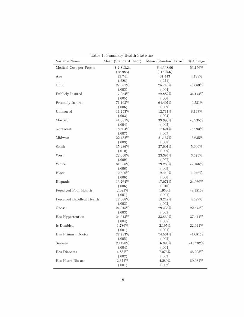
Table 1: Summary Health StatisticsVariable Name Mean (Standard Error) Mean (Standard Error) % Change

Medical Cost per Person $ 2,813.24 $ 4,308.66 53.156%(58.986) (116.656)

Age 35.744 37.443 4.739%(.228) (.271)

Child 27.587% 25.748% -6.663%(.003) (.004)

Publicly Insured 17.054% 22.882% 34.174%(.005) (.006)

Privately Insured 71.193% 64.407% -9.531%(.006) (.009)

Uninsured 11.753% 12.711% 8.147%(.003) (.004)

Married 41.631% 39.993% -3.935%(.004) (.005)

Northeast 18.804% 17.621% -6.293%(.007) (.007)

Midwest 22.432% 21.167% -5.635%(.009) (.008)

South 35.236% 37.001% 5.009%(.010) (.009)

West 22.630% 23.394% 3.373%(.009) (.007)

White 81.036% 79.280% -2.166%(.006) (.009)

Black 12.320% 12.449% 1.046%(.006) (.006)

Hispanic 13.764% 17.071% 24.030%(.006) (.010)

Perceived Poor Health 2.023% 1.959% -3.151%(.001) (.001)

Perceived Excellent Health 12.686% 13.247% 4.427%(.003) (.003)

Obese 24.015% 29.436% 22.575%(.003) (.005)

Has Hypertention 24.613% 33.830% 37.444%(.004) (.005)

Is Disabled 1.786% 2.195% 22.944%(.001) (.001)

Has Primary Doctor 77.733% 74.561% -4.081%(.005) (.005)

Smokes 20.420% 16.993% -16.782%(.004) (.004)

Has Diabetes 4.837% 7.076% 46.303%(.002) (.002)

Has Heart Disease 2.371% 4.289% 80.932%(.001) (.002)

18

Table 2: All Disease Price Indexes

YearDisease Based PriceIndex withoutComorbidities

Lowe Index withoutComorbidities

Disease Based PriceIndex withComorbidities

Lowe Index withCommorbities

1999 1.0155 1.0155 1.0162 1.01622000 1.1088 1.0445 1.1029 1.04522001 1.0959 1.0789 1.0760 1.08022002 1.1198 1.1113 1.1182 1.11302003 1.1790 1.1562 1.1738 1.15882004 1.2467 1.2016 1.2330 1.20462005 1.2841 1.2390 1.2406 1.24272006 1.3046 1.2772 1.2569 1.28192007 1.3640 1.3213 1.3196 1.32632008 1.3607 1.3548 1.3193 1.35992009 1.3725 1.3937 1.3231 1.39952010 1.3752 1.4335 1.3463 1.44052011 1.3588 1.4639 1.3041 1.47252012 1.3897 1.4970 1.3441 1.50662013 1.3981 1.5189 1.3569 1.52882014 1.4240 1.5413 1.3482 1.5523

19

Table 3: Disease Based Price Indexes from 1999 to 2014

PeriodLowe Index withoutComorbidities

Disease Based PriceIndex withoutComorbidities

Lowe Indexwith

Comorbidities

Disease Based PriceIndex withComorbidities

Infectious and parasitic dis-eases

1.535253 2.040713 1.540434 2.096055

Neoplasms 1.550261 1.01474 1.55176 0.983863Endocrine, nutritional,metabolic diseases andimmunity disorders

1.541666 1.148554 1.57693 1.194142

Diseases of the blood andblood-forming organs

1.562202 0.764136 1.585384 0.799676

Mental disorders 1.478756 0.922715 1.484428 0.826289Diseases of the nervous sys-tem and sense organs

1.46219 1.486762 1.477727 1.482008

Diseases of the circulatorysystem

1.554848 1.003742 1.573551 0.970491

Diseases of the respiratorysystem

1.547698 1.885904 1.558283 1.796676

Diseases of the digestive sys-tem

1.561487 1.600161 1.577627 1.607329

Diseases of the genitouri-nary system

1.526607 1.495045 1.530212 1.528959

Complications of pregnancy,childbirth and the puer-perium

1.530988 1.293316 1.530751 1.260413

Diseases of the skin and sub-cutaneous tissue

1.489018 1.503757 1.499381 1.491093

Diseases of the muscu-loskeletal system andconnective tissue

1.465533 1.340105 1.47472 1.204854

Congenital anomalies 1.532781 0.589359 1.535354 0.460634Certain conditions originat-ing in the perinatal period

1.640409 2.345117 1.640668 2.264331

Injury and poisoning 1.515745 1.697796 1.516295 1.643738Other conditions 1.505321 1.697717 1.522338 1.67472Residual codes and unclassi-fied

1.534528 1.545316 1.536986 1.573709

20

Table 4: Utilization Changes from 1996 to 2011

DiseaseInpatientHospital

Physicians Emergency

1 Infectious and parasiticdiseases

60% 10% 98%

2 Neoplasms -51% 4% -40%3 Endocrine, nutritional,and metabolic diseases andimmunity disorders

-54% -31% -27%

4 Diseases of the blood andblood-forming organs

-78% 1% 158%

5 Mental disorders -65% -50% -27%6 Diseases of the nervoussystem and sense organs

3% 1% 5%

7 Diseases of the circulatorysystem

-48% -39% -21%

8 Diseases of the respiratorysystem

23% -4% 33%

9 Diseases of the digestivesystem

-13% -10% 34%

10 Diseases of the genitouri-nary system

-15% 9% 58%

11 Complications of preg-nancy, childbirth, and thepuerperium

-20% -14% 4%

12 Diseases of the skin andsubcutaneous tissue

36% 12% 104%

13 Diseases of the muscu-loskeletal system and con-nective tissue

-1% -7% -35%

14 Congenital anomalies -81% -6% -78%15 Certain conditions origi-nating in the perinatal pe-riod

64% 483% 61%

16 Injury and poisoning 23% 23% 10%17 Other conditions 7% -26% 9%18 Residual codes and un-classified

17% 13% -56%

21

Table 5: Decomposition of Nominal Expenditure Growth

Disease

Ratio ofTotal Ex-penditures2012 toTotal Ex-penditures2002

Ratio ofPrice Index2012 to

Price Index2002

Ratio of2012

Populationto 2002

Population

Ratio of2012

PrevalenceRate to2002

PrevalenceRate

Ratio of2012 RealPer CapitaOutput to2002 RealPer CapitaOutput

1 Infectious and para-sitic diseases

1.425 1.481 1.091 0.987 0.893

2 Neoplasms 1.831 0.963 1.091 1.215 1.4353 Endocrine, nutri-tional, and metabolicdiseases and immunitydisorders

2.182 1.149 1.091 1.706 1.020

4 Diseases of the bloodand blood-forming or-gans

4.565 1.240 1.091 1.288 2.620

5 Mental disorders 1.829 0.958 1.091 1.336 1.3106 Diseases of the ner-vous system and senseorgans

1.469 1.292 1.091 1.052 0.991

7 Diseases of the circu-latory system

1.492 0.996 1.091 1.411 0.973

8 Diseases of the respi-ratory system

1.657 1.307 1.091 1.025 1.133

9 Diseases of the diges-tive system

1.881 1.281 1.091 0.887 1.517

10 Diseases of the gen-itourinary system

1.497 1.322 1.091 0.915 1.134

11 Complications ofpregnancy, childbirth,and the puerperium

1.683 1.183 1.091 0.948 1.376

12 Diseases of the skinand subcutaneous tis-sue

2.197 1.705 1.091 0.958 1.232

13 Diseases of themusculoskeletal sys-tem and connectivetissue

2.391 1.044 1.091 1.372 1.530

14 Congenital anom-alies

1.011 0.927 1.091 1.256 0.795

15 Certain conditionsoriginating in the peri-natal period

1.873 4.173 1.091 1.728 0.238

16 Injury and poison-ing

2.004 1.347 1.091 0.899 1.517

17 Other conditions 1.568 1.359 1.091 1.103 0.95818 Residual codes andunclassified

1.248 1.143 1.091 0.674 1.485

19 Dental diseases 1.324 1.485 1.091 0.950 0.86022