1

EXPERIMENTAL AND NUMERICAL INVESTIGATION OF UNSTEADY FLOWS IN A HIGH SPEED THREE STAGES

COMPRESSOR

N. Gourdain1, X. Ottavy2 and A. Vouillarmet2

1Computational Fluid Dynamics Team, CERFACS, Toulouse, 31057, France, Nicolas.Gourdain@cerfacs.fr

2Fluid Mechanics and Acoustic Lab., Ecole Centrale Lyon, Ecully, 69130, France, Xavier.Ottavy@ec-lyon.fr , Andre.Vouillarmet@ec-lyon.fr

ABSTRACT This study takes place in the frame of a research project to better understand the flow that

develops in a multistage high pressure compressor. The present paper focuses on the unsteady effects induced by rotor-stator interactions. Two complementary approaches are considered to increase data reliability and investigation capacity. First the flow is computed by the mean of a numerical approach, considering a 3D unsteady RANS flow solver. Then experimental data are used to validate and enhance the database. Results show that a good estimation of the mean flow features is obtained with the numerical model, even if some discrepancies are also observed, especially when regarding the transport of information along the axial distance. Detailed investigations of the flow at design and off-design conditions are then presented with the objective to underline the role of rotor-stator interactions.

NOMENCLATURE C mean blade axial chord h distance from the hub H height of the vein m spatial mode (=2π/λ) R number of rotor blades S number of stator blades Rpi total-to-total pressure ratio Rti total-to-total temperature ratio Q arbitrary quantity Q’ temporal fluctuation of the quantity Q y+ normalized wall distance α flow angle between axial and tangential velocities γ specific heat ratio (=1.4) φ normalized mass flow λ spatial wave number θ azimuthal angle ψ relative error (between steady and unsteady solutions) Ω rotation speed INTRODUCTION

2

To answer to the objectives in terms of pollutant emissions and economical constraints, the design of the next engine generation points toward compact, high efficiency and large operability configurations. An increase in performances of the critical components like the compressor is thus a necessary step, but many difficulties have to be overcome to achieve this challenging goal. First, an increase of the compressor efficiency can be obtained by means of a surge margin reduction. But it can be done only if a better understanding of the aerodynamic instabilities is reached. Secondly, a compact design means a shorter axial distance between blades rows which implies stronger flow unsteadiness and stronger rotor-stator interactions. Unfortunately, these unsteady flow effects that take place in a modern gas turbine engine are still not well understood, especially in a multistage compressor. It is well established that overall performances of a compressor are also strongly dependent on the flow behaviour near end walls (Domercq and Escuret, 2007). Furthermore, the compressor operability is also largely influenced by the tip clearance dimension (Inoue et al., 2004). The impact of these flows is not easy to estimate, resulting in an increase of the surge margin and thus an increase of the engine specific fuel consumption. Many authors such as Crook et al. (1993} and Hoying (1996) have clearly shown that the tip leakage regions exhibit usually the first signs of instabilities for most of the subsonic and transonic compressors. Indeed, a better description of the flow that develops near the casing in a multistage compressor can give valuable information to design high efficiency and more stable compressors. Today two approaches are mainly available to obtain valuable data for studying unsteady effects in compressors. In one hand, a popular method is the numerical simulation that allows very high investigation possibilities for a reasonable cost. But the main drawback of this way is still its poor predictive capacity for very complex flows, especially in a multistage environment. In the other hand, experimental campaigns are very useful to validate numerical models and provide reliable data, but this approach induces a higher cost than numerical methods and is not well suited to study aerodynamic instabilities in a high pressure compressor. Indeed, an approach that combines numerical simulation and experimental data is a way to develop and the work presented in this paper falls under this philosophy.

These last few years, the development of numerical tools such as the Computational Fluid Dynamics (CFD) and high performance computers led to significant progress to study turbomachine flow problems. Numerical methods have also been proposed to reduce the cost of unsteady flow calculations. For example, the Adamczyk flow model (Adamczyk, 1984) is an alternative way between steady and unsteady Reynolds-Averaged Navier-Stokes (RANS) calculations. The simulation cost is lower than a full unsteady method but the deterministic stresses have to be modelled, adding a new difficulty not easy to overcome. Another approach is the phase-lag assumption that can be used to simulate rotor-stator interactions with the calculation of only one passage of each row (Erdos et al., 1977). Based on the Tyler and Sofrin relation (1962), the method is efficient to compute periodic flow but only two spatial periodicities can be described (usually one stage). More recently, the development of spectral methods (Gopinath et al., 2007) has proven to be a very efficient way to simulate periodic flows in a turbomachine stage and promising results have been obtained for multistage applications. However, this technique has a limited validity domain, around design conditions where frequencies and spatial wavelengths are known. Unfortunately, all these methods can not be used to describe the whole performance map of a multistage compressor since no assumption can be done on time and space scales, especially at near stall conditions. Few authors have recently shown that a good balance between a correct physical description and the calculation time can be found to simulate very complex unsteady flows. For example, Hathaway et al. (2004) have investigated the development of instabilities in a full helicopter multistage compressor and a simulation of a rotating stall phenomenon has been done by Gourdain et al. (2006) in a full subsonic compressor stage. Both studies have been performed by means of a 3D unsteady RANS method. A higher level in terms of very large system simulation has been reached by Schluter et al. (2005) with the simulation of a full aircraft gas turbine, using an inventive

3

RANS/LES coupling strategy. Indeed, the unsteady RANS approach is still the most appropriate method to describe the flow in a multistage compressor, at any operating point.

Based on this state of the art, it is proposed in this paper to investigate the unsteady flow in a three-stage compressor, with a particular interest for the flow near the casing. The method of investigation is based on numerical simulations and fine measurements that are jointly used to study the flow and the rotor-stator interactions. The main characteristics of the experimental facility and the numerical methodology, with a particular interest for the numerical parameters, are presented in the first section. The predictive capacity of the numerical approach for this kind of application is not yet well established. Indeed the numerical parameters are chosen without the help of experimental results, in order to assess the reliability of the numerical model. First a comparison of the unsteady flow simulation with a steady flow numerical solution is done to point out the necessity for taking into account unsteady effects. The comparison with experimental data is then presented in a second part for time averaged quantities, with the objective to assess the capacity of the unsteady flow simulation to reproduce the main flow features. Then more detailed investigations of the unsteady flows that develop near the casing are presented and analyzed in a third section by means of a spectral analysis. The paper focuses on two operating points, at design and off-design conditions. Finally, useful information is pointed out for the numerical tool validation dedicated to complex unsteady flow simulation in a multistage environment. Moreover, this study will also help designers to better understand and estimate the role of the unsteady effects on the compressor performances.

INVESTIGATION METHODOLOGY

Experimental facility The test case considered for this study is a research multistage compressor dedicated to aero-

thermal and aerodynamic studies. This 3½-stages axial compressor, named CREATE (Compresseur de Recherche pour l'Etude des effets Aérodynamiques et Technologiques) has been designed and built by Snecma. Its geometry and its rotation speed are representative of High Pressure Compressor median-rear blocks of modern turbojet engine. The number of stages was chosen in order to have a magnitude of the secondary flow effects similar to a real compressor, and to be within the rig torque power limitation. Snecma and the research team of the LMFA Laboratory have taken into account technological constraints coming from the experimental part of the project, very early in the compressor design. In order to have traversal probes between blade and vane rows, the axial gap was slightly increased compared to current compressors and an outer-case moving-rings technology was implemented to perform probe measurements in the circumferential direction at constant radius location. The circumferential periodicity of the whole machine (obviously 2π in general case with primary blade numbers) has been reduced to 2π/16 on the CREATE compressor, choosing the number of blades of each rotor and stator (Inlet Guide Vane -IGV- included) as a multiple of 16 (see Table 1). Consequently, measurements carried out over a sector of only 2π/16 (namely 22.5 degrees) contain all the spatial information (in the case of stabilized operating points) and are very useful when devoted to detailed studies, such as rotor-stator interaction analysis. The compressor, the inter-row measurement sections and an overview of the test stand are presented in Fig. 1.

The CREATE compressor is tested at Ecole Centrale de Lyon in LMFA Laboratory. The test stand is designed as an open loop. The ambient air is led into the compressor trough a settling chamber with a throttle that drops the inlet total pressure (0.74 of the atmospheric pressure) and allows decreasing the needed electric power. The rotors shaft is driven at the design speed of 11,543 rpm by a 2 MW DC-drive coupled with a gearbox. At this rotational speed, the Mach number at the tip of the first stage is 0.92. Indeed the flow is slightly transonic in the first stage and fully subsonic in the two last ones. The inlet total temperature is measured by 10 sensors in the settling chamber. The inlet total pressure is obtained with a Kiel probe in front of the compressor. Total pressure and total temperature probe rakes, located at six circumferential and 5 radial positions in the outlet

4

section upstream the discharge collector, give the exit flow conditions. A throttling valve is used downstream the collector to control the mass flow rate, which is measured using a Venturi nozzle (not presented in Fig. 1) located just before the exhaust of the test-rig.

Row IGV R1 S1 R2 S2 R3 S3 Number of blades per

row (for 2π) 32 64 96 80 112 80 128

Number of blades for 2π/16 2 4 6 5 7 5 8

Table 1: number of blades of the compressor rows

Cylindrical outer casing diameter = 0.52 m

Core Speed = 11,543 rpm Rotor 1 Tip speed = 313 m/s

Fig. 1: CREATE compressor and its test-rig at Ecole Centrale Lyon

A backscatter Laser Doppler Anemometer (LDA), designed and built by Dantec, was used to

perform all the measurements presented in this paper. Two pairs of beams (λ=488nm and λ=514.5nm) are used for measuring simultaneously two velocity components with lead to the determination of the axial and tangential velocity components. The focal length of the front lens is 250 mm. A diameter of 76µm and a length of around 0.9mm characterize the measurement volume. The signals were treated by two Dantec real-time signal analyzers.

The measurements were triggered with the rotation frequency of the machine, in such a way that the flow field is described either inside a single blade passage, or within several blade passages covering the circumferential periodicity of the whole machine. The data reduction process filters the random time scales of the turbulent flow. Thus, the unsteadiness captured only relates to phenomena clocked with the rotor passing frequency.

The anemometer was carried on a six-axis robot allowing the location of the measurement point. This system prevents the optical assembly of the anemometer being sensitive to machine vibrations.

5

Due to the axial thrust and thermal dilatation of the machine, a procedure was defined for positioning the LDA control volume during compressor operation. The uncertainty of the location of any measurement point is then estimated to ±0.15 mm.

The compressor was seeded with a polydisperse aerosol of paraffin oil. The size of the particles at the outlet of the seeding generator was measured and its mean value is smaller than 1µm. Seeding was performed upstream of the settling chamber. In such a flow configuration (low centrifugal forces and moderated decelerations), Ottavy et al. (2001) proved that this technique was reliable.

The spatial and temporal discretizations for these measurements were chosen in agreement with the methodology applied by Ottavy et al. (2003) to minimize the interpolation errors in rotor/stator interaction analysis.

Once all the quantifiable uncertainties have been taken into account, the velocity component measurement error is about ±1.5 %. The velocity angles presented in this paper are calculated from the velocity components.

Numerical method The flow solver used is the elsA software that solves the RANS equations using a cell centred

approach on multi-block structured meshes (Cambier and Veuillot, 2008). To ensure a good precision, convective fluxes are computed with a third order Roe scheme considering a minimal Harten entropic correction (Roe, 1981) and diffusive fluxes are calculated with a second order centred scheme. A second order Dual Time Stepping (DTS) method is applied for the time integration (Jameson, 1991), considering 3200 iterations to discretize one rotation of the compressor at the design speed. The time marching for the inner loop is performed by using an efficient implicit time integration scheme, based on the backward Euler scheme and a scalar LU-SSOR method (Yoon and Jameson, 1987). Convergence acceleration techniques such as the local time stepping method are also used. To reach a converged state, the number of sub-iterations for the inner loop is defined to obtain at least two orders of reduction for the residuals magnitude. The turbulent viscosity is computed with the two equations model of Wilcox (1988) based on a k-omega formulation and the flow is assumed to be fully turbulent since the Reynolds number based on the chord is around 106.

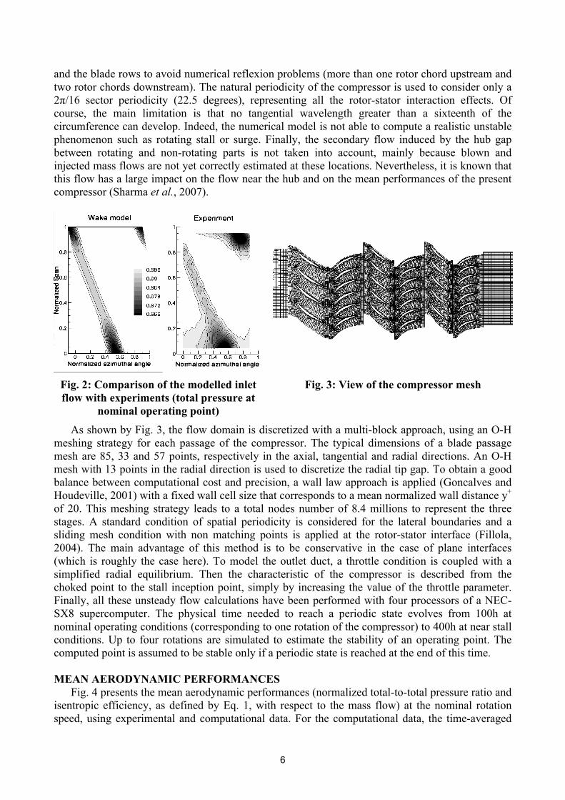
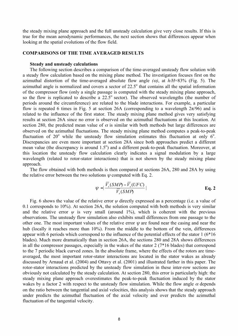
For practical reasons of computation time, the whole experimental domain can not be simulated. First the IGV is not represented but is taken into account with an analytical model. It is assumed that the flow distortion generated by the IGV is mainly induced by the presence of wakes. This behaviour is modelled according to the self similarity law of Lakshminarayana and Davino (1979) that describes the spatial evolution of wakes with a simple Gaussian function. Experimental data obtained at the nominal operating point are then used to fit the model constants as the circumferential wake extension L and the total pressure deficit ΔPwake. A comparison of the model with experiments is presented Fig. 2. As it can be shown, the wake model is able to reproduce the main features of the inlet flow, especially at mid-span. However, differences are observed near the hub and can be explained by a high temperature recirculation flow in the facility that is not considered by the analytical law. The wake model is then used to define the upstream injection condition through the values of total pressure Pt and total temperature Tt. As a first approximation the flow angle α is considered constant in the azimuthal direction. The turbulence intensity was measured with a single hot wire and is about 2% in the section 25A out of the wakes of the IGV. For the calculation this turbulence intensity was set to 1% (the experimental value was not known at this time).

Second, it is assumed that a good description of the deterministic stresses is the most important parameter to compute correctly the flow at stable conditions, meaning the duct length has no impact on the compressor performances and stability (Gourdain et al., 2005). Indeed only a part of the inlet and outlet ducts is modelled but a sufficient distance is considered between the boundary conditions

6

and the blade rows to avoid numerical reflexion problems (more than one rotor chord upstream and two rotor chords downstream). The natural periodicity of the compressor is used to consider only a 2π/16 sector periodicity (22.5 degrees), representing all the rotor-stator interaction effects. Of course, the main limitation is that no tangential wavelength greater than a sixteenth of the circumference can develop. Indeed, the numerical model is not able to compute a realistic unstable phenomenon such as rotating stall or surge. Finally, the secondary flow induced by the hub gap between rotating and non-rotating parts is not taken into account, mainly because blown and injected mass flows are not yet correctly estimated at these locations. Nevertheless, it is known that this flow has a large impact on the flow near the hub and on the mean performances of the present compressor (Sharma et al., 2007).

Fig. 2: Comparison of the modelled inlet flow with experiments (total pressure at

nominal operating point)

Fig. 3: View of the compressor mesh

As shown by Fig. 3, the flow domain is discretized with a multi-block approach, using an O-H meshing strategy for each passage of the compressor. The typical dimensions of a blade passage mesh are 85, 33 and 57 points, respectively in the axial, tangential and radial directions. An O-H mesh with 13 points in the radial direction is used to discretize the radial tip gap. To obtain a good balance between computational cost and precision, a wall law approach is applied (Goncalves and Houdeville, 2001) with a fixed wall cell size that corresponds to a mean normalized wall distance y+ of 20. This meshing strategy leads to a total nodes number of 8.4 millions to represent the three stages. A standard condition of spatial periodicity is considered for the lateral boundaries and a sliding mesh condition with non matching points is applied at the rotor-stator interface (Fillola, 2004). The main advantage of this method is to be conservative in the case of plane interfaces (which is roughly the case here). To model the outlet duct, a throttle condition is coupled with a simplified radial equilibrium. Then the characteristic of the compressor is described from the choked point to the stall inception point, simply by increasing the value of the throttle parameter. Finally, all these unsteady flow calculations have been performed with four processors of a NEC-SX8 supercomputer. The physical time needed to reach a periodic state evolves from 100h at nominal operating conditions (corresponding to one rotation of the compressor) to 400h at near stall conditions. Up to four rotations are simulated to estimate the stability of an operating point. The computed point is assumed to be stable only if a periodic state is reached at the end of this time.

MEAN AERODYNAMIC PERFORMANCES

Fig. 4 presents the mean aerodynamic performances (normalized total-to-total pressure ratio and isentropic efficiency, as defined by Eq. 1, with respect to the mass flow) at the nominal rotation speed, using experimental and computational data. For the computational data, the time-averaged

7

unsteady flow calculation (UFC) is compared with a steady mixing plane approach (SMP) (Denton, 1979). All the data presented in this figure are normalized with respect to the maximum experimental value. That means the mass flow is expressed as a fraction of the experimental chocked mass flow. The pressure ratio and the isentropic efficiency are normalized by the experimental maximum pressure ratio and efficiency respectively. The uncertainties are indicated for experimental data with horizontal and vertical bars. As an example for the nominal operating point, these uncertainties are equalled to 0.46%, 0.17% and 0.32% for the mass flow, the pressure ratio and the efficiency respectively.

Eq. 1

The locations of the experimental probes which give the total pressures and temperatures have

been reproduced in the numerical flow fields and the same averages have been used so as to compare experimental and numerical results properly.

Fig. 4: Mean aerodynamic performances - Pressure ratio (left) and isentropic efficiency

(right) The comparison of numerical results with the experimental measurements shows that the flow

blockage is slightly over predicted by the simulations (relative error is 2%) but the stability limit is better estimated (relative error is 1%), outlining the robustness and the predictive capacity of the numerical model for mean aerodynamic values since the prediction of the surge line position is usually a challenging feature for numerical flow solver. The shapes of the total-to-total pressure ratio and efficiency curves are also correctly represented by the simulations. However the isentropic efficiency is over predicted at most of the simulated operating point and a discrepancy of 1.5% is observed between the maximum experimental and numerical efficiencies. Taken into account the flow recirculation between rotating and fix disks is probably a way to achieve a better prediction of this compressor feature, since it is expected such flow effects will reduce the overall efficiency. Moreover, the mesh grid used for this study is not sufficiently fine to compute the smallest details of the flow which could also have an influence on the losses level. Another approximation is the inlet boundary condition that represents only a part of the IGV flow, meaning that the inlet flow characteristics are possibly not properly modelled, especially near the hub.

Despite of these differences, this comparison shows clearly that the presented steady and unsteady numerical simulations are able to reproduce the mean flow characteristics in this three-stage compressor, with a good agreement at near stall conditions. In this compressor configuration,

8

the steady mixing plane approach and the full unsteady calculation give very close results. If this is true for the mean aerodynamic performances, the next section shows that differences appear when looking at the spatial evolutions of the flow field. COMPARISONS OF THE TIME AVERAGED RESULTS

Steady and unsteady calculations The following section describes a comparison of the time-averaged unsteady flow solution with

a steady flow calculation based on the mixing plane method. The investigation focuses first on the azimuthal distortion of the time-averaged absolute flow angle (α), at h/H=83% (Fig. 5). The azimuthal angle is normalized and covers a sector of 22.5o that contains all the spatial information of the compressor flow (only a single passage is computed with the steady mixing plane approach, so the flow is replicated to describe a 22.5o sector). The observed wavelengths (the number of periods around the circumference) are related to the blade interactions. For example, a particular flow is repeated 6 times in Fig. 5 at section 26A (corresponding to a wavelength 2π/96) and is related to the influence of the first stator. The steady mixing plane method gives very satisfying results at section 26A since no error is observed on the azimuthal fluctuations at this location. At section 280, the predicted mean value of α is similar with both methods but large differences are observed on the azimuthal fluctuations. The steady mixing plane method computes a peak-to-peak fluctuation of 20o while the unsteady flow simulation estimates this fluctuation at only 6o. Discrepancies are even more important at section 28A since both approaches predict a different mean value (the discrepancy is around 1.5o) and a different peak-to-peak fluctuation. Moreover, at this location the unsteady flow calculation clearly indicates a signal modulation by a large wavelength (related to rotor-stator interactions) that is not shown by the steady mixing plane approach.

The flow obtained with both methods is then compared at sections 26A, 280 and 28A by using the relative error between the two solutions ψ computed with Eq. 2.

Eq. 2

Fig. 6 shows the value of the relative error ψ directly expressed as a percentage (i.e. a value of 0.1 corresponds to 10%). At section 26A, the solution computed with both methods is very similar and the relative error ψ is very small (around 1%), which is coherent with the previous observations. The unsteady flow simulation also exhibits small differences from one passage to the other one. The most important values of the relative error ψ are found near the casing and near the hub (locally it reaches more than 10%). From the middle to the bottom of the vein, differences appear with 6 periods which correspond to the influence of the potential effects of the stator 1 (6*16 blades). Much more dramatically than in section 26A, the sections 280 and 28A shows differences in all the compressor passages, especially in the wakes of the stator 2 (7*16 blades) that correspond to the 7 periodic black curved zones. In the absolute frame, where the effects of the rotors are time-averaged, the most important rotor-stator interactions are located in the stator wakes as already discussed by Arnaud et al. (2004) and Ottavy et al. (2001) and illustrated farther in this paper. The rotor-stator interactions predicted by the unsteady flow simulation in these inter-row sections are obviously not calculated by the steady calculation. At section 280, this error is particularly high: the steady mixing plane approach overestimates the peak-to-peak fluctuation induced by the stator wakes by a factor 2 with respect to the unsteady flow simulation. While the flow angle α depends on the ratio between the tangential and axial velocities, this analysis shows that the steady approach under predicts the azimuthal fluctuation of the axial velocity and over predicts the azimuthal fluctuation of the tangential velocity.

9

Based on this conclusion, the numerical results presented in the following parts of the paper and compared with experimental data are only related to the unsteady flow numerical simulation. The main objective is not only to assess the capacity of the unsteady flow numerical simulation to reproduce the mean flow features, by taking into account the mean unsteady effects, but also to quantify and understand the role of the unsteadiness.

Fig. 5: Azimuthal evolution of the time averaged velocity angle α at h/H=83%

Fig. 6: Relative error between the time-averaged unsteady flow simulation and the steady flow

simulation (axial velocity) Time and tangential averaged radial flow evolutions The radial evolutions of the angle between axial and tangential velocities α are compared at

different axial locations. In both experimental and unsteady calculation cases, all the data are time and space averaged by using the same procedure (note that the density is not accessible with LDA measurements; the averages are then weighted by the axial velocity instead of the axial momentum). Fig. 7 shows this quantity at nominal operating conditions while Fig. 8 corresponds to the near stall conditions.

Globally these comparisons point out that the simulation is able to reproduce the correct shape of the experimental curves at mid-span and near the casing. However, the simulation also clearly fails to predict the flow in some particular regions.

First, the flow that develops near the rotor hubs is not well estimated by the numerical method (see sections 26A and 27A of Fig. 7). Comparisons show that there is always an over prediction of the velocity angle due to the secondary flow that is not well taken into account by the simulation. Another reason is also that the flow angle near the hub at the compressor inlet is not well reproduced by the injection model, leading to a different flow near the hub in the two first rotors.

10

Section 26A Section 27A

Section 28A Section 280

Fig. 7: Radial evolution of the mean velocity angle α (nominal operating point, Φ=0.96)

Section 27A Section 28A

Fig. 8: Radial evolution of the mean velocity angle α (near stall point, Φ=0.90)

Second, the flow behind the second stator is less correctly estimated near the casing than behind

the rotors since the angle is largely over predicted by the simulation (see Fig. 7, section 280). One reason is that the flow at this location is strongly affected by the flow generated by upstream rows. This information is not well transported in the compressor by the simulation, probably because the numerical scheme is too dissipative, and thus does not interact strongly with the local flow.

Finally, at near stall conditions, the simulation correctly predict the flow at section 27A (behind the second rotor) while it shows a different behaviour from the experiments at section 28A (behind the last rotor). Experimental observations point out a similar evolution of the velocity angle α from the nominal to the near stall operating point (same shape but with a different magnitude) but the simulation predicts a large separation near the casing of the last rotor that led to a modification of

11

the shape curve above h/H=60%, with an important increase of the flow angle α (Fig. 8, section 28A).

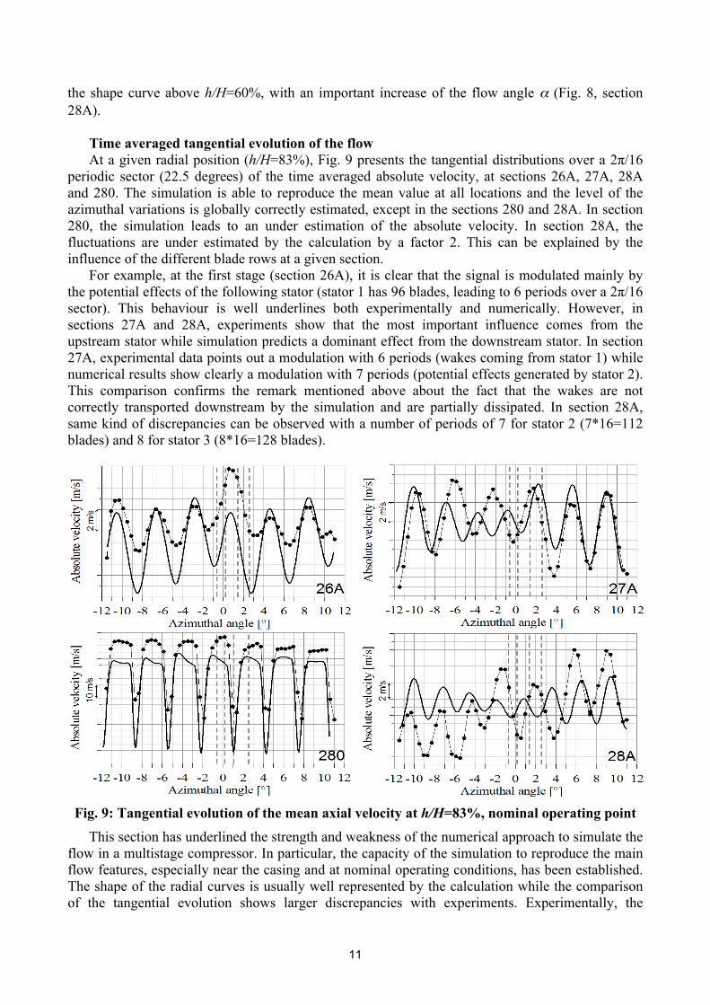
Time averaged tangential evolution of the flow At a given radial position (h/H=83%), Fig. 9 presents the tangential distributions over a 2π/16

periodic sector (22.5 degrees) of the time averaged absolute velocity, at sections 26A, 27A, 28A and 280. The simulation is able to reproduce the mean value at all locations and the level of the azimuthal variations is globally correctly estimated, except in the sections 280 and 28A. In section 280, the simulation leads to an under estimation of the absolute velocity. In section 28A, the fluctuations are under estimated by the calculation by a factor 2. This can be explained by the influence of the different blade rows at a given section.

For example, at the first stage (section 26A), it is clear that the signal is modulated mainly by the potential effects of the following stator (stator 1 has 96 blades, leading to 6 periods over a 2π/16 sector). This behaviour is well underlines both experimentally and numerically. However, in sections 27A and 28A, experiments show that the most important influence comes from the upstream stator while simulation predicts a dominant effect from the downstream stator. In section 27A, experimental data points out a modulation with 6 periods (wakes coming from stator 1) while numerical results show clearly a modulation with 7 periods (potential effects generated by stator 2). This comparison confirms the remark mentioned above about the fact that the wakes are not correctly transported downstream by the simulation and are partially dissipated. In section 28A, same kind of discrepancies can be observed with a number of periods of 7 for stator 2 (7*16=112 blades) and 8 for stator 3 (8*16=128 blades).

Fig. 9: Tangential evolution of the mean axial velocity at h/H=83%, nominal operating point

This section has underlined the strength and weakness of the numerical approach to simulate the flow in a multistage compressor. In particular, the capacity of the simulation to reproduce the main flow features, especially near the casing and at nominal operating conditions, has been established. The shape of the radial curves is usually well represented by the calculation while the comparison of the tangential evolution shows larger discrepancies with experiments. Experimentally, the

12

influence of the previous blade rows is responsible of a large modulation of the tangential signal while the simulation found mainly a local contribution with only a small impact of the previous blade rows. Thus, the main limitation of the numerical model is probably its capacity to transport the information along a long axial distance, meaning interactions between non adjacent blade rows are weaker than those experimentally observed.

UNSTEADY FLOW ANALYSIS

The analysis presented in the following section focuses on the unsteadiness that develops in the compressor. It is chosen to consider only the flow angle temporal fluctuations α’ to point out the unsteady aerodynamic behaviour of the flow. While it is straightforward to compare time averaged results, the comparison between unsteady numerical and experimental data is a bit more complicated, especially when defining a common origin for the time. As a first approximation, it is chosen to use the location of the rotor wakes to calibrate the time origin.

Investigation at the nominal operating point Investigations are led at the interfaces between rotor and stator blade rows at a given radial

position, chosen near the casing (h/H=83%), and at the nominal operating point (Φ=0.96). It is a challenging location for the numerical flow solver since strong interactions occur at this place between upstream wakes, potential effects and the tip leakage flow. For clarity reasons, flow angle fluctuations with respect to the time and the azimuthal direction are presented for only three sections (26A, 28A and 280) in Fig. 10, Fig. 11 and Fig. 12 respectively. The time is plotted over the whole compressor temporal periodicity normalized by 2π/16Ω, and the azimuthal angle covers a sector from -11.5 to 11.0 degrees, namely the whole compressor spatial periodicity. In the bottom of these figures, the flow angle fluctuations are also presented at four azimuthal locations, corresponding to the white horizontal lines plotted on the iso-countour map and to the vertical dotted lines in Fig. 9.

Section 26A This section corresponds to the rotor-stator interface at the first compressor stage, so it is a good

candidate to understand the observed phenomena since no influence comes from upstream blade rows (except from the IGV). As shown by Fig. 10, the numerical simulation computes the same flow structure than observed by experiments. The transport of the rotor wakes (white strips) is correctly computed and local interactions between the rotor wakes and the stator potential effects are well highlighted. As it can be shown the wake shape is very well reproduced by the simulation. When compared with experimental data, there is no error for the simulated wake thickness and only a slight under estimation (1 degree) exists for the value of α' inside the wake. Moreover, both datasets shows a constant shape of the wakes (amplitude and thickness) at the different investigated azimuthal locations. However, small discrepancies are observed outside the wakes, such as a small decrease of the flow angle fluctuations. Experiments show this decrease just before the wake while the simulation predicts the same phenomenon just after the wake and not at the same azimuthal position (see the fluctuations for θ=2.56°). Once again, this difference could be explained by the injection condition that does not reproduce perfectly the behaviour of the IGV and its influence on the angle of the flow entering in the rotor 1.

Section 28A As expected, the differences between simulation and experiments are larger at the section 28A

(Fig. 11). Experimental observations show a mean increase with respect to the section 26A of 60% in the flow unsteadiness, while numerical simulation predicts no or only a small increase. As in the section 26A, the increase of the flow angle is associated to a deficit of the relative velocity in the rotor wakes, but the relative velocity deficit is stronger in section 28A because it combines the

13

wakes of the rotor 3 and the rotor 2. In the experimental case, these wakes are clocking in a way that they superimpose their influences. That leads to higher levels of fluctuations and slightly increase the thickness of the zone associated to the wakes. In the case of the CFD, the discrepancies already observed for the flow angles downstream the rotor 3 (Fig. 7, section 28A at 83% span) explain that the trajectory of the wakes of the rotor 3 will not be the same in both experimental and CFD cases. The higher value of the CFD flow angle leads to the fact that the wakes of the rotor3 arrive a bit sooner in section 28A compared to the experimental case. This is what explains the 2 bumps in the CFD case, leading to a larger combined wakes structures with lower amplitude.

Section 280 The flow at this location is mainly driven by the second stator wakes and the third rotor

potential effects. As shown by Fig. 12, the simulation is able to reproduce the experimental flow features, as wakes and rotor-stator interactions modes (diagonal black stripes). It is also pointed out by all the datasets that the unsteadiness is very small outside the stator wakes while the signal registered inside a stator wake (at θ=0.96o) clearly shows an increase of the flow fluctuations. The combination between the rotor potential effects and the stator wakes lead to this very strong increase of the unsteadiness. From the previous observations, it is now well established that rotor-stator interactions modes have a strong influence on the flow behaviour, especially at section 280. To analyze these interaction modes, a Discrete Fourier Transform (DFT) is done, considering a (periodic) spatial signal of the flow angle fluctuations. Both experimental and numerical signals are interpolated at identical equally spaced azimuthal positions with a linear method. Fig. 13 shows the results of the DFT in terms of amplitude and phase, for experimental and numerical data.

To better understand the results obtained with this post-processing, the model of Tyler and

Sofrin (1962) is used to predict the development of a spatial mode m (Eq. 3) and its related rotation speed (Eq. 4). The sign of the mode m indicates the direction of its rotation with respect to the rotor rotation. This model also predicts a constant rotation speed Ωm and constant modal amplitude. For this application, the considered system is a periodic sector with the second stator (S=7) and the third rotor (R=5) which corresponds to the section 280. Eq. 3

Eq. 4

with n, b: integers Fig. 13 shows very good agreements between simulation and experiments, at this operating

point. First, simulation predicts correctly that mode #2 has the dominant effect on the flow. By using Eq. 3 it is easy to show that this mode is the result of the interaction between the stator 2 and the rotor 3 (with n=1, b=-1). Eq. 4 shows also that the theoretical rotation speed of this mode is 5ΩR, which is the observed numerical and experimental mean rotation speed. Other spatial modes are also correctly predicted by the simulation, such as the modes #9 (n=1, b=-2) and #12 (n=1, b=1). However the amplitude of the spatial mode #5 (n=1, b=0) is slightly over estimated by the simulation.

Second, the experimental and numerical phase angle analysis shows clearly that not only the

amplitude of the spatial modes are not constant with respect to the time (as already shown by Arnaud et al. 2004 and Bulot et al. 2007) but also their rotation speeds, which highlight the limitations of the Tyler and Sofrin model.

14

As an illustration, the phase angle fluctuations have been plotted in Fig. 14 for the mode #12. Experimental and numerical results indicate a similar level of fluctuations and clearly show that the phase angle oscillates reaching its higher levels at around 80% of the full temporal period. Even if a definitive explanation is not proposed at this time, it is highly probable that the interactions between spatial modes and the viscous effects could produce the observed effects.

Conclusions of the flow analysis at the nominal operating point are that upstream rows have a

large influence on the local flow in this multistage compressor, and that the simulation seems to transport only a limited part of this information. A short modal analysis has been done to highlight the rotor-stator interaction modes in section 280, showing that complex phenomena are involved in the development of these flow features. While the model of Tyler and Sofrin is able to compute the mean value of these interactions modes (such as the mean rotation speed and the mean wave number), it clearly failed to estimate the instantaneous rotation speed and amplitude of a given spatial mode.

Fig. 10: Temporal and spatial evolution of the flow angle fluctuations at h/H=82.2% (section

26A, nominal operating point)

15

Fig. 11: Temporal and spatial evolution of the flow angle fluctuations at h/H=83.7% (section

28A, nominal operating point)

Fig. 12: Temporal and spatial evolutions of the flow angle fluctuations at h/H=82.7% (section

280, nominal operating point)

16

Fig. 13: Amplitude and phase from the DFT of a flow angle fluctuation signal at h/H=82.7%

(section 280, nominal operating point)

Fig. 14: Phase angle fluctuations with respect to the time for the spatial mode #12 at

h/H=82.7% (section 280, nominal operating point)

Investigation at the near stall operating point A similar work is done at a near stall operating point (Φ=0.90), but for clarity and space

reasons, the analysis is presented only for the section 280 which represents the inlet condition of the last stage. This axial position is of a great interest at this mass flow since both experimental and

17

numerical data indicates the last stage exhibits the first sign of aerodynamic instabilities. The axial fluctuations generated by rotor-stator interactions are responsible for a tip leakage flow pulsation and both experimental and numerical data show that highest axial fluctuations are observed in the last stage. Indeed the unsteady flow blockage that periodically occurs near the rotor 3 leading edge is found to be a good candidate to trigger the surge. Fig. 15 presents the evolution of α’ with respect to the time and the azimuthal angle. Comparison of the numerical data with measurements points out discrepancies such as the level of unsteadiness inside the stator wakes. As mentioned before, the interaction between potential effects and wakes is responsible of the unsteadiness at this location. While experiments show a flow behaviour similar from nominal to near stall operating conditions, the simulation clearly over predict the influence of the rotor 3 potential effects. Moreover, a stator boundary layer separation is observed only numerically. These observations explains the higher level of unsteadiness predicted by the simulation (+25%) at position θ=0.96°.

As previously, a DFT is done, considering a spatial signal of the flow angle fluctuations. Fig. 16

presents the results of this post processing in terms of amplitude and phase, and for experimental and numerical data. Experiments shows that mode #2 is the dominant mode while simulation fails to estimate the development of the spatial mode and over predicts the influence of the spatial mode #5 (linked to the rotor 3). However, the simulation correctly estimates the contribution of other spatial modes such as mode #9 and mode #12 that corresponds to interaction between the stator 2 and the rotor 3. The phase angle of the mode #12 also exhibits a decrease of the temporal fluctuations.

Fig. 15: Temporal and spatial evolution of the flow angle fluctuations at h/H=83.7% (section

280, near stall operating point)

18

Fig. 16: Amplitude and phase from the DFT of a flow angle fluctuations signal at h/H=82.7%

(section 280, near stall operating point)

CONCLUSIONS The work presented in this paper is done following the philosophy that using experimental and

numerical approach is a very promising way to understand the flow physics that develop in a multistage compressor. However, from the numerical point of view it requires an unsteady model that is still costly in terms of computational resources while experimental campaigns have to obtain very fine and accurate unsteady measurements using high-cost rigs. The presented comparisons clearly show that the main flow features are correctly simulated even if some technological effects (such as the hub recirculation flow) are not taken into account. Another conclusion is that the numerical model is able to reproduce the local physic but also under estimate the interaction between upstream and local flows. The main reason is that the numerical model is too dissipative and a large part of the flow information is lost before it interacts with the other blade rows. This point has to be improved, especially if the description of a compressor with a long axial distance and multi-stage is required. A simple modal analysis has then been conducted to analyze numerical and experimental unsteady data. The results have been compared with the Tyler and Sofrin theoretical model, showing very interesting phenomena. While the theoretical model correctly predicts the development of the mean features of the rotor-stator modes, it fails to estimate the instantaneous rotation speed of the spatial modes, which is largely modulated by local fluctuations. The interest of the modal analysis is also to propose a reliable method to chose the time origin and suppress the time lag between experimental and numerical data.

A perspective of this work will be the improvement of the inflow condition by taking into account the whole experimental boundary conditions (and not only the IGV wakes) since this study

19

has clearly shows the large influence of the inflow on the first stage behaviour, up to mid-span. Other points of interest will be the reduction of the dissipation by using a lower dissipative numerical scheme and by increasing the number of mesh point to reach the mesh convergence state.

ACKNOWLEDGEMENTS

The authors are grateful to SNECMA for permission to publish results for the CREATE compressor. The experimental part of this work is supported by SNECMA Moteurs and SPAé. Special thanks to G. Halter, P. Krikorian, H. Navière, B. Paoletti and A. Willier for their technical works in the experimental part at LMFA. The authors are also grateful to CNRS, Région Rhône-Alpes and French Research Ministry in providing grants for metrology purchase. The computational results were obtained using the elsA software, developed by ONERA and CERFACS. Many thanks to Marc Montagnac (CERFACS) and Michel Gazaix (ONERA) for developing efficient algorithms that were been used in this study.

REFERENCES Adamczyk, J.J., “Model Equation for Simulating Flows in Multistage Turbomachinery”, Technical Memorandum 86869, NASA, USA, 1984

Arnaud, D., Ottavy, X., Vouillarmet A., “Experimental Investigation of the Rotor-Stator Interactions, within a High Speed, Multi-Stage, Axial Compressor. Part 2 – Modal Analysis of the Interactions”, 49th ASME TURBO EXPO 2004, ASME paper GT2004-53778, Vienna, June 14-17, 2004.

Bulot, N. and Trébinjac, I., "Impeller-Diffuser Interaction: Analysis of the Unsteady Flow Structures Based on their Direction of Propagation", Journal of Thermal Science, vol. 16 N°3, pp 193-202, 2007

Cambier, L. and Veuillot, J.P., “Status of the elsA CFD Software for Flow Simulation and Multidisciplinary Applications”, 46th AIAA Aerospace Science Meeting and Exhibit, AIAA 2008-664, Reno, USA, 2008

Crook, A.J., Greitzer, E.M., Tan, C.S. and Adamczyk, J.J., “Numerical Simulation of Compressor Endwall and Casing Treatment Flow Phenomena”, J. of Turbomachinery, Vol. 115, pp 501-512, 1993

Denton, J.D. and Singh, U.K., “Time Marching Methods for Turbomachinery Flow Calculations”, VKI Lecture Series 1979-7, Von Karman Institute, Belgium, 1979

Domercq, O. and Escuret, J.-F., “Tip Clearance Effect on High-Pressure Compressor Stage Matching”, J.of Power and Energy, Vol. 221, pp. 759-767, 2007

Erdos, J.I, Alzner, E. and McNally, W., “Numerical Solution of Periodic Transonic Flow Through a Fan Stage”, AIAA Journal, Vol. 15, pp. 1559-1568, 1977

Fillola, G., Le Pape, M.-C. and Montagnac, M. “Numerical simulations around wing control surfaces”, 24th international congress of the aeronautical sciences ICAS, Yokohama, Japan, 2004

Goncalves, E. and Houdeville, R., “Reassessment of the wall functions approach for RANS computations”, Aerospace Science and Technology, Vol. 5, pp. 1-14, 2005

Gopinath, A., Van Der Weide, E., Alonso, J.J., Jameson, A., Ekici, K. and Hall, K.C., “Three-Dimensional Unsteady Multi-Stage Turbomachinery Simulations using the Harmonic Balance Technique”, 45th AIAA Aerospace Sciences Meeting and Exhibit, AIAA Paper 2007-0892, Reno, USA, 2007

Gourdain, N, Burguburu, S. and Leboeuf, F., “Rotating Stall Simulation and Analysis in an Axial Compressor”, 17th International Symposium on Air Breathing Engine, ISABE paper 2005-1138, Munich, Germany, 2005

Gourdain, N., Burguburu, S., Michon, G.-J., Ouayahya, N., Leboeuf, F. and Plot, S., “About the Numerical Simulation of Rotating Stall Mechanisms in Axial Compressors”, ASME Turbo Expo, ASME paper GT2006-90223, Barcelona, Spain, 2006

20

Hathaway, M.D. and Herrick, G. and Chen, J. and Webster, R., “Time Accurate Unsteady Simulation of the Stall Inception Process in the Compression System of a US Army Helicopter Gas Turbine Engine”, Proceedings of the DoD Users Group Conference, pp182-193, Washington, DC, USA, 2004

Hoying, D.A., “Blade Passage Flow Structure Effects on Axial Compressor Rotating Stall Inception”, PhD thesis, Massachusetts Institute of Technology, Cambridge, USA, 1996

Inoue, M., Kuroumaru, M., Yoshida, S., Minami, T., Yamada, K. and Furukawa, M., “Effect of Tip Clearance on Stall Evolution Process in a Low-Speed Axial Compressor Stage”, ASME Turbo Expo, paper GT2004-53354, Vienna, Austria, 2004

Jameson, A., “Time Dependent Calculations Using Multigrid, with Applications to Unsteady Flows Past Airfoils and Wings”, AIAA Journal, AIAA-91-1596, 1991

Lakshminarayana, B. and Davino, R., “Mean velocity and decay characteristics of the guide vane and stator blade wake of an axial flow compressor”, Gas Turbine Conference and Exhibit and Solar Energy Conference, ASME paper 79-GT-9, San Diego, USA, 1979

Ottavy, X., Trébinjac, I., Vouillarmet A., “Analysis of the Inter-row Flow Field within a Transonic Axial Compressor : Part 2 - Unsteady Flow Analysis”, 45th International Gas Turbine & Aeroengine Technical Congress, ASME Paper 2000-GT-0497, Journal of Turbomachinery Vol. 123 n°1, pp.57-63., Münich, Jan. 2001.

Ottavy, X., Trébinjac, I., Vouillarmet A., Arnaud, D., “Laser Measurements in High Speed Compressors for Rotor-Stator Interaction Analysis”, proceedings of ISAIF 6th, Shanghaï, April 2003, International Journal of Thermal and Fluid Sciences, Nov. 2003.

Roe, P.L., “Approximate Riemann Solvers, Parameter Vectors and Difference Schemes”, J. of Computational Physics, Vol. 43, pp. 357-372, 1981

Schluter, J., Apte, S., Kalitzin, G. and Van Der Weide, E., “Large-scale integrated LES-RANS simulations of a gas turbine Engine”, Annual Research Briefs, Stanford University, 2005

Sharma, V., Aupoix, B., Schvallinger, M. and Gaible, H., “Turbulence Modelling Effects on Off-Design Predictions for a Multi-Stage Compressor”, 18th International Symposium on Air Breathing Engine, ISABE paper 2007-1183, Beijing, China, 2007

Tyler, J.M. and Sofrin, T.G., “Axial Flow Compressor Noise Studies”, SAE Transactions, Vol. 70, pp. 309-332, 1962

Wilcox, D.C., “Reassessment of the Scale-Determining Equation for Advanced Turbulence Models”, AIAA Journal, Vol. 26, pp. 1299-1310, 1988

Yoon, S. and Jameson, A., “An LU-SSOR Scheme for the Euler and Navier-Stokes Equations”, AIAA 25th Aerospace Sciences Meeting, AIAA-87-0600, Reno, Nevada, USA, 1987