Ris0-R-1116(EN)

Unsteady Airfoil Flows with Application to Aeroelastic Stability

Jeppe Johansen

DISTRIBUTION OF THIS DOCUMENT IS UNLIMITED FOREIGN SALES PROHIBITED

&JL—

Ris0 National Laboratory, Roskilde, Denmark September 1999

REC

EIVE®

m t*

a

OSTI

DISCLAIMER

Portions of this document may be illegible in electronic image products. Images are produced from the best available original document.

Ris0-R-1H6(EN)

Unsteady Airfoil Flows with Application to Aeroelastic Stability

Jeppe Johansen

Ris0 National Laboratory, Roskilde, Denmark September 1999

Abstract The present report describes numerical investigation of two-dimensional unsteady airfoil flows with application to aeroelastic stability. The report is di­vided in two parts. Part A describes the purely aerodynamic part, while Part B includes the aeroelastic part.

In Part A a transition prediction algorithm based on a simplified version of the e" method is proposed. The approach is based on the idea that instability data from the stability theory are computed for a variety of flow conditions. The instability data are stored in a database from which the information can be ex­tracted by interpolation. The input to the database are laminar integral boundary layer parameters. These are computed from an integral boundary layer formu­lation coupled to a Navier-Stokes flow solver. The model is validated on a zero pressure gradient flat plate flow, and compared to an empirical one-step transition prediction method. Five different airfoils are considered at fixed angle of attack, and the flow is computed assuming both fully turbulent and transitional flow and compared with experimental data. In the case of unsteady airfoil flows four dif­ferent airfoils are investigated. Three oscillating in pitch and one in plunge. For comparison a semi-empirical dynamic stall model is employed on the same test cases. Additional implementation of arbitrary forcing has been conducted and validated.

Results indicate that using a transition model the drag prediction is improved considerably. Also the lift is slightly improved. At high angles of attack transi­tion will affect leading edge separation which again will affect the overall vortex shedding. If the transition point is not properly predicted this will affect the whole hysteresis curve. The transition model developed in the present work showed more stable predictions compared to the empirical transition model. The semi-empirical dynamic stall model predicts lift, drag, and moment characteristics acceptably well as long as vortex shedding is not present.

In Part B a simple three degrees-of-freedom (DOF) structural dynamics model is developed and coupled to the aerodynamics models from Part A. A 2nd order accurate time integration scheme is used to solve the equations of motion. Two airfoils are investigated: One is a 2 DOF NACA 0012 airfoil free to translate in normal direction and free to rotate around the quarter-chord. Both stable and unstable conditions are computed, and results are compared to a comparable study from the literature. Both aeroelastic models predict stable conditions well at low angle of attack. But at high angles of attack, and where unstable behaviour is expected, only the Navier-Stokes solver predict correct aeroelastic response. The semi-empirical dynamic stall model does not predict vortex shedding and moment correctly leading to an erroneous aerodynamic damping.

The second airfoil under consideration is a 3 DOF LM 2 airfoil, which can also vibrate in the edge-wise direction. An attempt to predict stall induced edge-wise vibrations is conducted. Both aeroelastic models predict comparable aeroelastic response where stable conditions are expected. At higher angles of attack, where the flow is separated, both models predict more dominant pitching motion, but no stall induced edge-wise vibrations were predicted with the present approach.

ISBN 87-550-2544-7 ISBN 87-550-2545-5(Internet) ISSN 0106-2840

Information Service Department • Ris0 • 1999

PrefaceThis thesis is submitted in partial fulfillment of the requirements for the Danish

Ph.d. degree at the Technical University of Denmark. The supervisors were Ass. Prof. Jens Nprkaer Sprensen, Institute for Energy Engineering, Technical Univer­sity of Denmark, and Senior Researcher Niels Nprmark Sgrensen, Wind Energy and Atmospheric Physics Dept. Risp National Laboratory, Denmark. I would like to thank them for qualified supervision and quidance, and to you Niels, for letting me take so much of your time. It has been very inspiring.

. The thesis is based on numerical work carried out from 1st. of October 1995 to 31st. of March 1999 at Ris0 National Laboratory, Denmark and at the Department of Energy Engineering, Technical University of Denmark.

I would like to thank my colleagues at Ris0 National Laboratory and my fellow students at the Institute for Energy Engineering, Technical University of Denmark. I would also like to thank John Ekaterinaris who guided me trough the initial stages of my Ph.D. period, while he was a visiting researcher at Ris0 National Laboratory.

Finally, I would like to thank the people at the National Wind Technology Center, National Renewable Energy Laboratory, Colorado, USA for making my six month stay in the fall of 1997 a life time experience. Especially Mike Robinson, who made the stay possible and Kirk Pierce, who let me use his Beddoes-Leishman code.

The thesis is divided in two parts. The first Part A concerns the purely aero­dynamic part, while Part B concerns the aeroelastic part.

After an overall introduction in chapter 1 the aerodynamic part is introduced in chapter 2. The flow solver, EllipSys2D, turbulence, and the developed transition model are described in chapter 3 together with validation of the model. Chapter 4 describes results of flows past airfoils at fixed angles of attack.

In chapter 5 unsteady airfoil flows and semi-empirical dynamic stall models are discussed followed by chapter 6 where results of various unsteady airfoil flows are presented.

Part B begins with chapter 7 with an introduction to aeroelasticity, followed by chapter 8 where the aeroelastic model is defined together with the time integra­tion and the coupling between the aerodynamic model and the structural model. Finally, chapter 9 describes a number of aeroelastic test cases followed by overall conclusions in chapter 10.

March 1999

Jeppe Johansen

mRis0-R-1116(EN)

Contents

Preface Hi

Contents it)

Nomenclature vi

1 Introduction 11.1 Research Objectives 2

Part A: Aerodynamic Modeling s

2 Introduction to Aero dynamics 3

3 Aero dynamic Model 43.1 Navier-Stokes code (EllipSys2D) 43.2 Turbulence Modeling 43.3 Laminar/Turbulent Transition Modeling 63.4 Simplified e" model 93.5 Model Validation 11

4 Results of Flow past Fixed Airfoils 144.1 DU-91-W2-250 174.2 S809 234.3 FX66-S-196 VI %4.4 NACA 63-425 254.5 RIS0-1 26

5 Flow past Periodically Moving Airfoils 285.1 EllipSys2D 305.2 Semi-empirical Dynamic Stall Models 305.3 Beddoes-Leishman Model 31

6 Results of Flow past Periodically Moving Airfoils6.1 NACA 0015 336.2 RIS0-1 356.3 S809 396.4 NACA 23-010 47

Part B: Aero elastic Modeling so

7 Introduction to Aero elasticity 50

8 Aeroelastic Model 538.1 Structured Model 538.2 Time Integration Scheme 548.3 Verification of Time Integration Scheme 558.4 Coupling with Flow Solver 56

33

iv Ris0-R-1116(EN)

9 Results of Aeroelastic Flows 589.1 Validation 589.2 NACA 0012 (2 DOF) 609.3 LM 2 (3 DOF) 69

10 Conclusions 7710.1 Recommendations for Further Research 78

References 80

Appendix 82

A Discretization of Boundary Layer Equations

B Beddoes-Leishman Dynamic Stall Model 85

83

Ris0-R-1116(EN) v

NomenclatureGreek Letters

aaoQfiOCeq

065*S3€

7tr

Ar,PvVtnwL0aUxOJy4>PTij

Tw9ecCqj Ce> Cy

Angle of attack Initial angle of attack Imaginary part of spatial wave number Equivalent angle of attack Prandtl-Glauert compressibility factor Boundary layer thicknes Displacement thickness Kinetic energy thickness DissipationIntermittency functionReal and imaginary part of eigenvalue, AMass ratioTotal viscosity (laminar + turbulent)Eddy viscosity Vorticity, Rotational Speed Specific dissipation rate Pitch natural frequency, [rad/s]Edge-wise natural frequency, [rad/s] Flap-wise natural frequency, [rad/s] Amplitude of perturbation, numerical error DensityReynolds Stresses Skin friction Momentum thickness Stream-wise coordinate Complex damping ratio Structural damping ratios

Roman Letters

a.c.ahbcc.g.CdCdCfClCmCncvCte.a.fFuF2hH=Sih- = st

Aerodynamic centerNon-dimensional distance between e.a. and mid-chordNon-dimensional semi-chordChordCenter of gravity Dissipation coefficient Drag coefficient Skin friction coefficient Lift coefficient Moment coefficient Normal force coefficient Pressure distribution Tangential force coefficient Elastic axis Frequency, [Hz]Blending functions Non-dimensional plunging amplitude Shape factorKinetic energy shape factor

VI Ris0-R-1116 (EN)

khikpkpilMPrraTCgReSSttTu,vue[7oo

y*w-x,yxax/cX%ry+

Turbulent kinetic energy Lead-lag reduced frequency Pitch reduced frequency Plunge reduced frequency Mixing length Mach number Local pressure RadiusNon-dimensional radius of gyration Non-dimensional distance between c.g. and mid-chord Reynolds numberNon-dimensional distance in semi-chords Strouhal number Time Period [s]Local velocities Boundary layer edge velocity Free stream velocity Non-dimensional velocity Wind speed, Work Global coordinatesNon-dimensional distance between e.o. and c.g. Non-dimensional horizontal distance from leading edge Transition point location Non-dimensional distance from surface

Abbreviations

2-D Two-DimensionalB-L Beddoes-LeishmanCFD Computational Fluid DynamicsDOF Degrees-Of-FreedomDNS Direct Numerical SimulationFEM Finite Element MethodsIBLF Integral Boundary Layer FormulationLCO Limit Cycle OscillationsLES Large Eddy SimulationNREL National Renewable Energy LaboratoryNS Navier-StokesODE Ordinary Differential EquationPISO Pressure-Implicit with Splitting of OperatorsPSE Parabolized Stability EquationsBANS Reynolds Averaged Navier-StokesSIMPLE Semi-Implicit Method for Pressure-Linked EquationsSST Shear Stress TransportSUDS Second Order Upwind Differencing

Ris0-R-1116(EN) vu

viii Ris0-R-1116 (EN)

1 IntroductionThe term Unsteady Airfoil Flow relates to the unsteady forces created on two- dimensional (2-D) aerodynamic airfoil shaped bodies subjected to a fluid flow. The flow causes pressure and friction on the body surface, which again results in forces and moments acting on the body. When the airfoil moves due to either forced motion or elastic deformation the incidence, or the angle of attack, changes with time. This causes the forces to change resulting in dynamic effects. Another phenomenon that also greatly influences the dynamic forces is the stream-wise pressure gradient in the boundary layer. With increasing adverse pressure gradient the boundary layer will eventually separate from the surface causing additional dynamic changes in forcing. At high angles of attack of an airfoil, where large adverse pressure gradients are present on the suction side separation can take place and vortices can be shed causing the airfoil to stall, i.e. an abrupt decrease in lift. For a periodic varying incidence, the forces and moments will exhibit hysteresis effects due to the difference in separation for increase compared to decrease in angle of attack. These dynamic stall effects are highly non-linear.

Airfoil shaped bodies are utilized in a number of industries. The most widely known are aircraft, helicopter, wind turbine, and turbomachinery industries, where proper prediction of airfoil characteristics are of major importance. Unsteady air­foil flows and dynamic stall prediction methods used by the industry are largely based on empirical or semi-empirical approaches, which are fast and rather ac­curate where non-linear effects are not too great. But increased development in aircraft and wind turbine aerodynamics creates demand for a more detailed in­formation of the non-linear unsteady loads, dynamic response, and aeroelastic stability, caused by dynamic airfoil motions, including dynamic stall effects.

Earlier on aerodynamic theory was mainly based on small disturbance theory. Using this theory the non-linear aerodynamic equations were linearized making the solution a possible task. This theory is valid for arbitrary unsteady incom­pressible motion of an airfoil. It has been proven quite applicable for unsteady flow in the attached region. By correcting the theory by Prandt-Glauert’s com­pressibility correction compressible effects can be investigated as well. A second approach for investigating arbitrary motion of subsonic airfoil flow is employing a superposition of indicia! response functions, i.e. Fourier-integral superposition of theoretical results for simple harmonic oscillations. This method has also been extended to take non-linear aerodynamic effects into account. Finally, investiga­tion of detailed non-linear aerodynamics has recently (within the last couple of decades.) been possible using Computational Fluid Dynamics, (CFD).

Aeroelasticity is a discipline where mutual Interaction between aerodynamic and elastic forces on lifting surfaces is investigated. Aeroelastic theory has developed since the first airplanes began to exhibit undesired vibrations during flight. The first aeroelastic theory was, as aerodynamic theory, based on small disturbance theory in order to linearize the problem. Theodorsen coupled his aerodynamic the­ory to the typical section (a two degrees-of-freedom airfoil section) and made the first aeroelastic stability investigations, Bisplinghoff et al., ref. [4]. Later non-linear aerodynamic theories were applied together with structural finite element models (FEM) for flutter studies, and finally to examine the detailed non-linearities of the aerodynamics, CFD is used for fully coupled aeroelastic problems.

Due to advances in computational methods and computing power, the ability to solve the full unsteady Reynolds averaged Navier-Stokes equations have made

Ris0-R-1116(EN) 1

it feasible to investigate and solve the mysteries of unsteady airfoil flows. The present work contributes to this field by using CFD together with turbulence and transition modeling to investigate unsteady airfoil flow phenomena. By coupling a simple structural model to the CFD code it is possible also to investigate aeroe- lastic stability problems.

1.1 Research ObjectivesThe objectives of the present work are twofold. The first major objective is to de­velop a transition model suitable for modeling transition point locations in a fast and efficient way in 2-D flows. The model is based on linear stability theory and referred to as the e" model. The present approach is to solve the linear stability equation (the Orr-Sommerfeld equation) once and save the boundary layer stabil­ity data in a database. The database requires laminar boundary layer parameters as input. These are computed by an integral boundary layer equation approach on top of a 2-D incompressible Navier-Stokes (NS) solver. In this way boundary layer parameters can be computed without the difficulty of determining the boundary layer edge directly from a NS solver. The transition model is validated on flat plate flow and applied on airfoil flow together with an empirical transition model, the Michel Criterion, for comparison. Finally both fully turbulent and transitional computations are performed on unsteady airfoil flows, i.e. dynamic stall.

The second major objective of the present work is to investigate aeroelastic stability using a NS solver. A simple three degrees-of-freedom (DOF) structural dynamics model is developed and coupled to the flow solver. A 2nd order accurate implicit Crank-Nicolsen method is used to solve the system of coupled non-linear equations.

A minor objective is the implementation and application of a semi-empirical dynamic stall model, the Beddoes-Leishman dynamic stall model, and use it as a fast alternative to, and for comparison with the NS solver. This model is also coupled to the 3 DOF structural model for comparing aeroelastic computations.

Finally the aeroelastic models are applied on two airfoils i.e. a 2 DOF NACA 0012 airfoil and a 3 DOF wind turbine airfoil, the 18 % thick LM 2 airfoil.

2 Ris0-R-1116(EN)

Part A:Aerodynamic Modeling

2 Introduction to AerodynamicsOn stall regulated wind turbines large regions of separated flow will occur during operation at high wind speeds. This approach controls the power output by ex­ploiting that lift force decreases when the wind turbine blade stalls and thereby power output and loads are limited. The overall three-dimensional flow on a rotor is a very complex unsteady flow depending on a variety of parameters. These are wind speed, wind shear, atmospheric turbulence, yaw angle, rotational speed, rotor radius, the overall layout of the blade, i.e. twist, taper, and thickness distribution, rotor radius, and finally the airfoil shape, i.e. thickness, camber, smoothness of surface, leading edge thickness, roughness insensitivity, blunt/sharp trailing edge, etc. During stalled operation aerodynamics is highly non-linear and hysteresis ef­fects will occur. Some of these effects will also take place on a two-dimensional (2-D) non-rotating wing exhibiting unsteady motion. Effects which are of major importance in predicting 2-D dynamic stall effects include the ability to properly predict airfoil characteristics; lift, drag, and moment coefficients, which highly de­pend on correct prediction of separation. A second effect is transition from laminar to turbulent flow in the boundary layer. If turbulence intensity of the incoming flow is low and the airfoil is designed to maintain laminar flow on part of the airfoil surface, the point where transition takes place is important to predict correctly, since it affects the skin friction and the laminar separation.

The following chapters of part A describes the aerodynamic models employed in the present work to solve some of the mysteries of unsteady airfoil flows. Chapter 3 describes the incompressible Navier-Stokes flow solver EllipSys2D together with turbulence and transition modeling. A transition model based on linear stability theory is proposed and validated on a flat plate flow. Computations of flow past fixed angle of attack airfoil sections are presented in chapter 4. Unsteady airfoil flow and various results are described in chapters 5 and 6, respectively.

Ris0-R-1116(EN) 3

3 Aerodynamic Model3.1 Navier-Stokes code (EllipSys2D)The CFD results determined in the present study are computed using EllipSys2D, an incompressible general purpose Navier-Stokes solver in 2-D. It is developed by Michelsen, ref. [29], [30] and Sorensen, ref. [42], and is a multiblock finite vol­ume discretization of the Reynolds Averaged Navier-Stokes equations in general curvilinear coordinates. The code uses primitive variables (u,v, and p). The in­compressible continuity equation is

dujdxj 0,

and the incompressible Reynolds Averaged Navier-Stokes equations are

(1)

dui dui 1 dp-m+Ujd^ + pd^

adxj

dui duAd^+d^J (2)

Solution of the momentum equations is obtained using a second order upwind differencing scheme, (SUDS). For incompressible flow an additional equation is needed for the pressure, and the standard practice is to derive a pressure equation by combining the continuity equation with the momentum equation. The momen­tum and pressure equations are then used in a predictor-corrector fashion using the SIMPLE algorithm by Patankar, ref. [32] for steady state calculations. For the unsteady calculations the PISO method by Issa, ref. [18] is applied. The resulting time integration is 1st order accurate in time.

The steady state calculations are accelerated by the use of a three level grid sequence and a local time stepping, while the transient calculations employ single grid technique with global time stepping in order to retain temporal accuracy.

At the end of the Ph.D. period an experimental version of the EllipSys2D code was further developed at Risp to employ a dual time stepping algorithm to fur­ther decrease the computational time during unsteady computations. The idea is that an additional level of iteration is introduced in order to get rid of numerical stability problems using large time steps. Within one physical time step a number of subiterations are performed assuming steady-state condition. This additional subiteration allows the code to take a physical time step of nearly any size as long as the overall flow features are captured. The computational cost is approximately a factor five more expensive per time step, but it is possible to take time steps two orders of magnitude larger than the original unsteady computations. So the technique reduces the computational time with a factor of % 20. This algorithm is used for some of the more recent computations. The methods is described in more detail in Rumsey et al., ref. [38].

3.2 Turbulence ModelingThe key discipline when computing turbulent flow using CFD is the modeling of turbulence. Due to the very large spectrum of length and time scales a full simu­lation of all present turbulent scales is impractical. For simple flow configurations and low Reynolds numbers this can be done using Direct Numerical Simulation (DNS), which can only be used in 3-D flows and would require unrealisticly large computational resources for the flow configurations considered here. For turbulent airfoil flows two kinds of turbulence modeling is currently available. They are Large Eddy Simulation (LES) where the inhomogeneous turbulence is resolved using the

4 Ris0-R-1116(EN)

Navier-Stokes equations, and the very small homogeneous scales are modeled us­ing a proper ’’subgrid scale model”. The second kind of turbulence modeling is based on the Reynolds Averaged Navier-Stokes equations (BANS), and is a phe­nomenological approach. In the present work only computations based on the BANS approach are conducted.

There are a number of BANS turbulence models which are placed in two cate­gories, the 1st order models and the 2nd order models. In the 1st order models the Reynolds stresses, ry, are related directly to the mean velocity field, while the 2nd order models solve balance equations for the Reynolds stresses. 1st order closure models are based on the Boussinesq approximation which assumes that the princi­pal axes of the Reynolds-stress tensor coincide with those of the mean strain rate tensor at all points in the turbulent flow. The coefficient of the proportionality is the eddy viscosity, i/j.

Three different kinds of 1st order models are available.

In the algebraic model, vt oc l2 , the mixing length l is described by an algebraic equation determined empirically by the flow configuration, while the velocity gradient is related to the mean flow.

• In the one-equation model, the mixing length is supplemented with a trans­port equation of a turbulent quantity, usually the turbulent kinetic energy, k, (Then i/t oc Ik?) but also the eddy viscosity, vt, or the modified turbulent Reynolds number, vRet, can be used.

• In the two-equation model, i>t is obtained through the solution of two balance equations: usually one for k and another for either the dissipation, e, which gives vt oc ^-, or for the specific dissipation rate, w, which gives vt oc

In most engineering applications involving a fully turbulent flow with only weak stream-wise pressure gradients and small curvature effects, turbulent quantities can be predicted well using conventional 1st order turbulence models. For flows with adverse pressure gradients and especially for separated flows, most 1st order turbulence models fail to give proper predictions.

In airfoil flows, which, due to the curvature of the surface, contains areas with relatively large stream-wise pressure gradients, the choice of a turbulence model is important. For high incidences the circulation of the airfoil causes severe adverse pressure gradients on the suction side, which often leads to separation and vortex shedding. Because of this turbulence models with the ability to take history effects into account, i.e. transport of Reynolds stresses, are considered for the present study.

In EllipSys2D a number of turbulence models are implemented, but during pre­vious work done at Risp the k—u SST (Shear Stress Transport) model by Menter, ref. [27], has proven very useful for 2-D airfoil flow. The following subsection de­scribes the k — u SST model.

k — ui SST turbulence model

The k—u SST model by Menter, ref. [27], is a hybrid of the original k—u model by Wilcox, ref. [52] and the standard k—e model by Jones and Launder, ref. [19]. It is known that the Wilcox k—u model is superior to the k — e model in wall bounded flows. The k — u model does not involve damping functions at the wall and allows simple Dirichlet boundary conditions to be specified. This simplicity makes the model more numerically stable than other two-equation models. Furthermore the behavior of the k — u model in the logarithmic region is superior to that of the k — e model in equilibrium adverse pressure gradient flows. In the wake region of the boundary layer, the k — u model has to be abandoned in favor of the k — e

Ris0-R-1116(EN) 5

model, because of its sensitivity to the ffeestream values, w#. The k—e model does not suffer from this dependency and this model is utilized in the free shear layer away from the surface. To achieve these desired features in the different regions the k — e model is transformed to a k — w formulation, and the two versions are coupled using a blending function, Fl, in the boundary layer.

An additional feature of the k—u> SST model is the modification of the eddy vis­cosity to take into account the transport of the maximum Reynolds shear stresses. The eddy viscosity is given by

Vt moz(oicv; | Cl | Fz) ’

oi being a constant, k is the turbulent kinetic energy, fl is the vorticity, and Fz is a blending function different from Fl. This definition secures that for adverse pres­sure gradient boundary layer flows, production of k is larger than its dissipation (or Cl > ai u>), or in other words that the eddy viscosity ut is kept smaller than in the original definition, leading to an earlier separation. The original formulation, z/t = £ is used in the rest of the flow. The two transport equations for k and w, respectively, are given by

dk dk , , . dk (4)and

, du tv dui n o 9-Qi+uniz: = aTTti*r-Pu'dxj k 13 dxj dxj

(fJ, + CTulH)9wdxj

(5)P,P*,<Tk,crw, and aU2 are model constants defined in Menter, ref. [27]. The blend­ing functions, Fi and Fz, are functions that varies from unity in a large part of the boundary layer and goes to zero at the boundary layer edge. (Here fi are kinematic viscosities.)

The k — u SST model is implemented in EllipSys2D by Sprensen, ref. [43], and all computations in the present report are computed using this model.

3.3 Laminar/Turbulent Transition ModelingComputation of flows over airfoils is a challenging problem due to the various complex phenomena connected with the occurrence of separation bubbles and the onset of turbulence.

In the case of low Reynolds number airfoil flows (Rec < O(106)), proper model­ing of the transition point location is crucial for predicting leading edge separation and skin friction. The transition prediction algorithm must be reliable since the transition point location may affect the termination of a transitional separation bubble and hence determine bubble size and associated losses. This again has a strong influence on airfoil characteristics, with drag being the most affected.

The airfoil flows under consideration in the present report are all at Reynolds numbers based on chord length varying from Rec = 1.0 x 106 to Rec = 3.0 x 10®. This range is typical for wind turbine applications. For these types of flow the laminar to turbulent transition is an important factor to take into account.

The transition from laminar to turbulent flow occurs because of an incipient in­stability of the basic flow field. Disturbances in the freestream, such as freestream turbulence or vorticity, enter the boundary layer as steady and/or unsteady fluctu­ations of the basic state. A variety of different instabilities can occur independently or together and the appearance of any type of instability depends on Reynolds number, wall curvature, surface roughness, and freestream turbulence intensity. The initial growth of these instabilities is described by linear stability theory. This

6 Ris0-R-1116(EN)

growth is weak and can be modulated by pressure gradients. As the amplitude grows, three dimensional and non-linear effects occur in the form of secondary instabilities. The disturbance growth is very rapid in this case and breakdown to turbulence occurs. The point of instability, Xinst, is defined as where the first in­stabilities occur, and transition takes place at Xtr, where the first turbulent spots appears. In Schlichting, ref. [39], the transition scenario is described. The region between the transition point and where the flow has become fully turbulent, xturb, is called the transition region.

If the initial instabilities are strong (e.g. high ffeestream turbulence or surface roughness) the growth of linear disturbances is by-passed and the linear theory fails to predict transition. In this case computations are usually made assuming fully turbulent flow, which is a fair and reasonable assumption.

The e” method is probably the most widely used transition prediction method and this will also be applied in the present study (see below). Besides linear theory, other approaches for modeling transition should be mentioned here. One method applies asymptotic theory. The theory allows the inclusion of non-linear effects stemming from non-parallel, quasi-parallel flows. Further information can be obtained from Cowley et al., ref. [8]. A more recent approach is the parabolized stability equations (PSE). This concept is related to the linear stability theory, except that the PSE method takes history effects into account and allows for analyzing forced modes, non-linear growth and secondary instabilities up to the breakdown stage. Further information can be obtained from Herbert, ref. [17].

In the present work, a transition prediction procedure based on a simplified en model has been developed and it is compared to a simple empirical model, the Michel Criterion.

Michel Criterion

A popular transition prediction model is the empirical criterion by Michel, ref. [28]. As shown by e.g. Ekaterinaris et al., ref. [11] and Mehta et al., ref. [26], this model gives fairly good results for many airfoil flows. The Michel criterion is a simple model based on experimental data on a flat plate with almost no pressure gradient and correlates local values of momentum thickness with position of the transition point. It simply states that transition onset location takes place where

where Regttr is the Reynolds number based on momentum thickness, and Rex,tr is the Reynolds number, based on the distance measured from the stagnation point.

en Method

The en method was originally proposed by Smith, ref. [40] and van Ingen, ref. [50]. It is based on linear stability analysis using the Orr-Sommerfeld equation to de­termine the growth of spatially developing waves.

Linear stability theory suggests that the unperturbed steady and parallel mean flow is superimposed with a time-dependent sinusoidal perturbation - the Tollmien- Schlichting waves. This results in the well known Orr-Sommerfeld equation, which is a 4th order linear eigenvalue problem in <j>, where <j> is the amplitude of the per­turbation. This equation determines whether spatially developing waves will be stable or unstable due to the amplification factor o%, which is the imaginary part of the spatial wave number. For positive a,- the waves are damped and for neg­ative a,- the waves are growing and the flow becomes unstable. In this way the

Ris0-R-1116(EN) 7

point of instability can be determined. This is defined as where at- = 0, i.e. neutral stability.

The en model predicts turbulence when the amplitude of the most unstable frequency exceeds the initial unstable amplitude by a factor e". In figure 1 the process of determining the n factor is depicted.

F,<F,

F x Re,

O;<0(Unstable]

Figure 1. Schematic representation of the neutral curve, the amplification factor a,, and the integrated N factor for a boundary layer with a constant value of shape factor H. Stock and Degenhart, ref. [45]

In the top graph of Figure 1 the neutral curve obtained from the Orr-Sommerfeld equation is shown, (a,- = 0). F is the reduced frequency, Res- is the Reynolds number based on displacement thickness, and is the amplification factor of the perturbations in spatial stability theory. Sweeping through the neutral curve for different values of F, F\, The N factor can be determined for each frequency using

rRes-N(Fi,Res>) = — I aidRes-, (7)

jRe‘nin

resulting in a number of N curves as the one depicted in the lower graph of figure 1. The envelope of all N curves results in a nmax curve, which can be used to determine the point of transition. The n factor is empirically determined from several experiments, and can vary from one flow situation to another. It is usually set at a value around 8-10. In the present work it is set at 9. i.e. when the amplitude of the most unstable spatially developing wave has increased by a

8 Ris0-R-1116(EN)

factor e9 ~ 8100. For farther details about the e" model see Arnal, ref. [3], Smith, ref. [40], and van Ingen, ref. [50].

3.4 Simplified en modelThere have been several successful attempts to apply simplified versions of the en method in combination with viscous-invisdd interaction algorithms (e.g. Drela and Giles, ref. [10] and Cebeci, ref. [6]).

In the present work a database on stability, with integral boundary layer pa­rameters as input, has been established, as suggested by Stock and Degenhart, ref. [45]. The approach is based on the idea that a discrete set of results to the Orr-Sommerfeld equation is representative for all possible laminar velocity pro­files and for all relevant disturbance frequencies. In the present work the instability data are stored in a database from which the relevant information can be extracted by interpolation. This database avoids the need for computing growth rates for each velocity profile.

The database is originally implemented by Petersen, ref. [33] using Falkner-Skan velocity profiles and is extended by Olesen, ref. [31] to include separated velocity profiles, based on the theory of Dini et al., ref. [9], which applies velocity profiles described by hyperbolic tangent functions. The final database was in previous work never validated properly, but during this work small errors were fixed and the database was ready for application.

As input to the database the laminar integral parameters such as displacement thickness, 6*, momentum thickness, 6, kinetic energy thickness, S3, boundary layer edge velocity, ue, together with Reynolds number base on chord length, Rec, are used. These are computed using an integral boundary layer equation approach combined with the Navier-Stokes solver.

Integral Boundary Layer Formulation

Input parameters for the database are laminar boundary layer parameters, S*,6, and S3 together with ue and Rec. This results in some difficulties. First, the deter­mination of boundary layer parameters using the NS solver is not accurate, since the boundary layer thickness is not well defined. Second, turbulence starting from the transition point influences the integral parameters upstream. This results in boundary layer parameters differing from their fully laminar value resulting in erroneous interpolation in the database. An alternative procedure is thus required for calculating these parameters.

The procedure chosen in the present study is a two equation integral boundary layer model based on dissipation closure.

The first of the two equations is the von Karman integral relation given by:

S+<2+<w=t- (8)

where H is the shape factor, £ is the stream-wise coordinate, and Cf is the skin friction coefficient. This equation is obtained by integrating the steady boundary layer equations with respect to the normal direction across the boundary layer. The second equation is a combination of eq. (8) and the kinetic energy thickness equation, and is given by:

(9)where H* is the kinetic energy shape parameter and Cd is the dissipation coef­ficient. For laminar flow, the two 1st order ordinary differential equations can be

Ris0-R-1116(EN) 9

solved with the following closure relationships for H*, Cf, and Cd respectively.

H* = 1.515 + 0.076^^, H< 4

H* = 1.515 + 0.040^=51!, H> 4 (10)

(11)

Reg = 0.207 + 0.00205(4 - H)5-5,H < 4

(12)

This model has successfully been used in viscous-inviscid interactive algorithm by Drela and Giles and for further details is referred to Drela and Giles, ref. [10].

To solve the two equations, (8) and (9), a third relation is necessary. By using the NS solver to compute the pressure at the surface and assuming no pressure variation across the boundary layer (pwait = Pe), ue can be determined from using the Bernoulli equation along a streamline. The two equations are then solved by a Newton-Raphson method.

Close to the stagnation point, where the skin friction varies dramatically and a small variation in skin friction factor causes a large variation in edge velocity, the equations are solved using a direct procedure (ue given - solving for 8 and H). When approaching separation, the direct procedure becomes ill-conditioned because a single edge velocity corresponds to two different skin friction factors. (One positive and one negative) By computing Cf using the NS solver, H can be computed using the closure relation, eq.(ll), and eqs. (8) and (9), can be solved inversely with 8 and ue as variables. Laminar separation takes place at H as 3.9. In the present implementation the inverse procedure is initiated before separation takes place, i.e. when H = 3.0

The computations need an initial value for the displacement thickness, 8, which is obtained using Thwaites’ method. Thwaites’ method is an empirical correlation between 8 and ue given by (White, ref. [51]).

Equations (8) and (9) are discretized using a 2nd order central differencing scheme and the descretized equations are given in appendix A.

Transition region

The extension of the transition region is obtained by an empirical model, suggested by Chen and Thyson, ref. [7]. This is a conceptually simple model that scales eddy viscosity by an intermittency function, varying from zero in the laminar region and progressively increases in the transition region until it reaches unity in the fully turbulent region. The intermittency function, jtr, is given by

v is the total viscosity (y = viam+vt). The modeling constant, G^tr was originally suggested to be 1200 for high Reynolds number flows. In order to take into account separation, especially for low Reynolds number flows, it was modified by Cebeci, ref. [6] to take the form

10 Ris0-R-1116(EN)

G^tr = 213[log(Eeatr) - 4.732]/3. (14)

The range at which this modification is valid is Rec = 2.4 x 105 to 2.0 x 106.

Solution Algorithm

The overall solution algorithm for the integral boundary layer equations is as follows:

1. The Navier-Stokes solver computes the overall flow field, i.e. u,v,p,k,w.

2. The direct procedure is applied.(a) As initial values the transition subroutine computes an edge velocity, ue

from the Bernoulli equation, the momentum thickness, 8 using Thwaites’ method, and the skin friction coefficient, Cf — Tw/(l/2pv%).

(b) The direct method uses ue as input to the integral boundary layer equa­tions and computes 8 and H using a Newton-Raphson method stepping in the stream-wise direction.

3. When H reaches 3.0, the inverse solution procedure is applied.(a) Hinverse is computed using the closure relation for eq. (11), and is

used as input to the integral boundary layer equations.(b) The inverse procedure computes 8 and ue using a Newton-Raphson

method stepping in the stream-wise direction.

4. The instability database are called at each boundary layer station with bound­ary layer parameters as input to investigate stability.

5. If the boundary layer is unstable, i.e. when n reaches 9, the transition point is determined and the computation is stopped.

3.5 Model ValidationTo validate the transition model and to exemplify the procedure of the model, steady flow over a flat plate is investigated, since this is a relatively simple tran­sitional flow. Almost no pressure gradient is present and a large amount of exper­imental data exist. The critical Reynolds number, Recr, is defined as the value where the flow turns from laminar to turbulent and it is a function of the turbu­lence intensity. For the present computation the turbulence intensity is in practice negligible.

The flat plate is modeled as a plate with a finite, but very small thickness. The leading edge is described as a parabola and the trailing edge is made by collapsing the two last points into one. The thickness of the plate is 0.002 chord lengths and the parabola is extended 10 thicknesses from the leading edge. The grid around the flat plate is a half O-grid made symmetric around the chord. The boundary condition at the symmetry line ensures symmetric flow conditions. In this way the number of grid points is reduced to half number of grid points. The grid has 144 grid points in the stream-wise direction and 72 in the normal direction, respectively. The inflow and outflow boundary of the grid is placed 1 chord length from the plate. The Reynolds number based on chord length is Rec = 4.0 x 106.

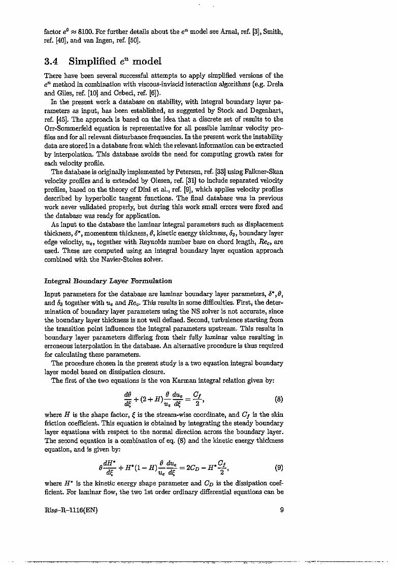
Figure 2 shows the momentum thickness, 8, the displacement thickness, 5*, and the skin friction factor, Cf, using the integral boundary layer formulation coupled to the NS solver, and compared with the exact solution for laminar flat plate flow given by Blasius. It should be noted here that the integral boundary layer computation is only computed until turbulence starts to occur, causing the values

Ris0-R-1116(EN) 11

IBLFBlasius

IBLFBlasius

Oe+OO

IBLFBlasius

x/c

Figure 2. Solution of integral boundary layer formulation (IBLF), represented by 6, 5*, and Cf and compared with exact solution by Blasius, Rec = 4.0 x 106.

to end at x/c = 0.57 (see later). The computed shape factor has the value of H = 2.59 which corresponds exactly to the theoretical laminar value. As seen the results are in good agreement with theory indicating that the integral boundary layer formulation gives good predictions for flows without stream-wise pressure gradient.

12 Ris0-R-1116(EN)

Intermittency fct. ---------

x/c x/c

Figure 3. Flow over a flat plate. Maximum n-factor, nmax, transition point loca­tion, xtr, a,nd intermittency function, jtr> -Rec = 4.0 x 106.

Figure 3 shows left the growth of the n factor, nmax, as one proceeds down­stream. The initial instability takes place around Xinst = 0.05 and the transition takes place where the n factor reaches the value 9, i.e. xtr — 0.57. The resulting transition point corresponds to a critical Reynolds number, Recr = 2.3 x 106. The right plot shows the intermittency function, jtr, determined by equation (13). It is seen that the flow is considered fully turbulent at xturb R* 0.85 corresponding to Returb — 3.4 x 106. The experimental value of the critical Reynolds number is given by Recr = 2.8 x 106 and the Reynolds number where the flow has be­come fully turbulent is Returb = 3.9 x 106, Schlichting, ref. [39]. The difference in Returb compared to the experimental value depends on the definition of fully turbulent since the intermittency function asymptotically approaches unity. The agreement is considered good. For comparison; using the Michel criterion results in Xtr = 0.50 -> Recr = 2.0 x 106. The extension of the transition region corresponds well with experiments.

Ris0-R-1116 (EN) 13

4 Results of Flow past Fixed Air­foilsThe present section describes the results for a number of fixed airfoils at different Reynolds numbers. The computations are made using EllipSys2D. After a descrip­tion of the grid generation, some general assumptions concerning the experimental data are discussed. For the first airfoil both steady and unsteady computations are made to verify the sufficiency of using steady computations for static airfoil flows. The rest of the airfoil computations are made assuming steady state conditions in order to take advantage of the local time-stepping acceleration algorithm. Solu­tion of the momentum equations is obtained using a 2nd order upwind difference scheme (SUDS) and the pressure-velocity coupling is obtained with the SIMPLE method.

Grid Generation

The computational grids are generated by the program HypGrid2D developed by Sorensen, ref. [44]. This is a hyperbolic grid generator. The topology used in the present work is an O-grid which has the advantage over C-grids that the cells in the wake are not as stretched. Furthermore the placement of the wake is avoided using an O-grid leading to a more general grid. A grid refinement study is made for all grids. The resulting grids for all airfoils are constructed to have a distance to the first gridline away from the surface corresponding to y+ % 0.5 in order to satisfactorily resolve the laminar sublayer. The outer boundary is around 16 chord lengths away from the airfoil. The number of grid points are 256 around the airfoil and 64 normal to the airfoil surface. The distribution of grid points around the airfoil surface was optimized for each airfoil due to the different geometries (i.e. leading edge curvature, camber, thickness, blunt/sharp trailing edge, etc.)

An example of a grid is shown in figure 4, which shows the grid around a DU- 91-W2-250 airfoil. At the bottom of figure 4 details of grid near the surface and at the blunt trailing edge are shown.

General Assumptions

Both fully turbulent and transitional computations, using both transition models, are made for comparison with experimental data. The experimental data comes from a variety of airfoils measured in different wind tunnels with different levels of turbulence intensity. If the turbulence intensity is low,(< 0.1%) and the airfoil is smooth the flow can be considered as being transitional. But if the turbulence intensity is too high, disturbances in the freestream can bypass the transition and generate turbulence further upstream. In this case a fully turbulent computation is expected to be closer to experimental data compared to a transitional compu­tation. Finally, some experiments are conducted with roughness elements placed on the airfoil leading edge. In this case turbulence is generated at the leading edge as a source. This flow configuration is not possible to predict with the present version of the code.

14 Ris0-R-1116(EN)

Figure 4- Grid around DU-91-W2-250 airfoil (top), and details showing grid reso­lution around the surface (left) and around the blunt trailing edge (right). 256 x 64 grid points.

Airfoils

The test cases chosen are airfoils which are mainly developed for wind turbine application, but also other airfoils are chosen where the flow parameters are com­parable, and the experimental data are considered as being of good quality. The airfoils are shown in figure 5.

Ris0-R-1116(EN) 15

DU-91-W2-250

-0.05 •

-0.1 •

S8090.15 -

-0.1 •

-0.15 ■

FX66-S-196 VI

NACA 63-425

-0.15 -

x/c

RIS0-1

0.05 •

Figure 5. Airfoils tested at fixed angels of attack.

16 Ris0-R-1116(EN)

The experimental data for the first three airfoils include measurements of the transition points. The first two, the DU-91-W2-250 and the S809, are airfoils designed for wind turbine applications, where no large difference between fully turbulent and transitional flow is expected, since they are designed to be roughness insensitive. The third airfoil, the FX66-S-196 VI, is a laminar airfoil where large difference between fully turbulent and transitional flow is expected. The NACA 63-425 airfoil was chosen as a high Reynolds number case. Finally, a third wind turbine airfoil, the RIS0-1 airfoil, measured in a high turbulence intensity wind tunnel is investigated.

Results are presented by lift and drag coefficients (Ci and Cj) as function of an­gle of attack, a, and pressure distributions, Cp, skin friction distributions, Cf, and transition point locations, xtr, and compared with experimental data, if available.

4.1 DU-91-W2-250The first airfoil considered is a dedicated wind turbine airfoil with a relative thick­ness of 25%. The Reynolds number based on chord length is Rec = 1.0 x 106. It is developed at the Delft University and tested in the low turbulence wind tunnel, Timmer and van Rooy, ref. [47]. The freestream turbulence level varies from 0.02% at 10 m/s to 0.1% at 90 m/s.

The experiments are conducted on an airfoil with smooth surface. Because of this it is assumed that the surface does not trigger turbulence until the lami­nar boundary layer becomes unstable and the flow experiences free transition to turbulence.

The problem about the unsteadiness of the flow and the ability of being able to compute an unsteady flow over a fixed airfoil with a steady procedure was first investigated. Six different angles of attack, varying from attached flow to highly separated flow were computed using the unsteady mode of EllipSys2D. The un­steady computations employ the PISO algorithm for the pressure-velocity coupling and a single grid technique with global time stepping in order to retain temporal accuracy. The non-dimensional time step used is At = 0.002. The results of the unsteady computations are shown in figure 6 assuming fully turbulent flow and transitional flow using two different transition prediction models, and compared with experimental data.

Figure 7 shows the lift and drag curves for the steady-state approach compared with experimental data.

As seen from the two figures 6 and 7 no particular difference is seen between the unsteady and the steady-state computations except for high angles of attack.

An extra consideration is the computational time. For attached flow (a = 3.574°) a fully turbulent converged steady state solution was obtained within rs 1000 iterations, while the unsteady converged solution was obtained after 8000 iter­ations corresponding to 16 non-dimensional sec. For separated flow (a = 15.190°) a periodic solution was obtained within 1500 iterations using the steady-state ap­proach, while a periodic solution was obtained within 13000 iterations using the unsteady approach. This corresponds to 26 non-dimensional sec. with a time step of At = 0.002.

Ris0-R-1116(EN) 17

fully turb. en model

Michel model Exp. data1.50 -

crry-o o o

Figure 6. Lift and drag curves using the unsteady approach. DU-91-W2-250 airfoil, Rec = 1.0 x 10®.

fully turb. en model

Michel model Exp. data

1.00 -

0.50 -

■cr—a™o—

Figure 7. Lift and drag curves using the steady-state approach. DU-91-W2-250airfoil, Rec = 1.0 x 10®.

18 Ris0-R-1116(EN)

The transition points were also determined during the experiment and computed values are shown in table 1 together with experimental data.

Table 1. Transition point locations on the DU-91-W2-250 airfoil atRec = 1.0 xlO6, (n.m. means not measured, a * indicate an accuracy of i0.05j.

xtr» p steady unsteadya exp en Michel en Michel

-4.652 0.61 0.48 0.60 - --0.027 0.52 0.43 0.49 - -3.574 0.48 0.41 0.43 0.41 0.417.686 0.42 0.36 0.36 0.37 0.369.225 0.38 0.13 0.32 0.12 0.319.742 0.36 0.086 0.30 0.089 0.2911.712 0.22 0.020 0.21 0.051 0.2115.190 n.m. 0.014 0.08 0.027 0.10xtrio%a steady unsteady

a exp en Michel en Michel-4.652 n.m. 0.36 0.41* - --0.027 n.m. 0.41 0.40* - -3.574 n.m. 0.46 0.45* 0.46 0.507.686 n.m. 0.50 0.48* 0.50 • 0.539.225 n.m. 0.51 0.50* 0.51 0.569.742 n.m. 0.51 0.51* 0.51 0.5411.712 n.m. 0.53 0.54* 0.53 0.5515.190 n.m. 0.54 0.57* 0.55 0.61

At low angles of attack the Michel model predicts xtr in good agreement with experiments, but the minor difference is not important as seen on the pressure distribution shown below in figure 8. Around maximum lift, a = 10°, the en model predicts transition close to the leading edge, while the Michel model again gives better predictions. Again no particular difference between the unsteady and the steady-state approach is observed.

Based on this investigation it is concluded that a steady-state computation is appropriate for this airfoil compared to accuracy and computational cost of employing an unsteady computation. The rest of the computations in this chapter is made employing EllipSys2D in the steady-state mode.

Experimental pressure distributions are available for six different angles of at­tack, and the corresponding steady-state computations are shown in figure 8. At high angles of attack the pressure distributions are snapshots taken where airfoil characteristics have averaged values in the periodic solution.

Ris0-R-1116(EN) 19

a = -0.027° a = 3574°

cn model ---------Michel model —■ 1

Exp. data »Michel model ——

Exp. data ®

2.00 •

a = 7.686° a =9.742°

Fully turb. ■■e" model ---------

Michel model 1 ■ Exp. data 6

Michel model -----Exp. data ®

Figure 8. Pressure distributions for six different angles of attack, DU-91-W2-250 airfoil, Rec = 1.0 x 106.

From the pressure distributions it is seen that for attached flow (a < 8°) the transitional computations predicts the pressure distribution very good. At a = 9.742° the Michel model is superior to the e" model, which is due to the better prediction of the transition point location on the suction side (see table 1). Using the Michel model at a = 11.712° the erroneous pressure distribution and resulting lift, even though the transition point prediction is good, is caused by a

20 Ris0-R-1116(EN)

later separation (x/csep = 0.88) compared to the fully turbulent and transitional computation using the e" model (x/csep = 0.60). Looking at the experimental data the separation point is actually earlier than predicted by the computations (%/c<;ep = 0.50). Finally, on the last pressure distribution at a = 15.190° a small laminar separation bubble is predicted at the leading edge using the Michel model. No such separation is seen in the experimental data indicating that transition is placed at the leading edge as predicted by the en method.

Figure 9 shows the computations of the skin friction distributions for the same angles of attack. Here the main observation is the large difference between fully turbulent and transitional computations, emphasizing the importance of transition point prediction when considering drag. A second note is the small separated regions present in the transitional computations on the pressure side right where transition takes place, indicating laminar separation. The relatively large concave surface on the pressure side increases possibility for separation and this laminar separation triggers turbulence. The laminar leading edge separation bubble is clear at a = 15.190°.

Unfortunately no experimental data were available, but the qualitative results are clear.

Ris0-R-1116(EN) 21

u

u

u

ass-0.027°0.020

Fully turb. cn model

Michel model0.015

0.010

-0.005

•0.010

x/c

a = 7.686°0.020

Fully hub. c° model

Michel model0 015

0.010

0.005

0.000

-0.005

-0.010

x/c

a =11.712°0.020

Fully turb. en model

Michel model

0.010

0.005

0.000

•0.005

-0.010

x/c

0.020Fully turb.

c" model Michel model

0.015

0.010

0.005

0.000

-0.005

•0.010

x/c

a= 9.742°0.020

Fully turb. e° model

Michel model0.015

0.010

0.005

0.000

-0.005

•0.010

x/c

a= 15.190'0.020

Fully turb. - 1c" model ---------

Michel model ■ —0015

0.010

0.005

0.000

-0.005

•0.0100.00 0.20 0.40 0.60 0.80 1.00

x/c

Figure 9. Skin friction distributions for six different angles of attack, DU-91-W2- 250 airfoil, Rec = 1.0 x 10®.

22 Ris0-R-1116(EN)

4.2 S809The S809 airfoil is a 21 % wind turbine airfoil designed at National Renewable Energy Laboratory (NREL), Colorado, USA, by Somers, ref. [41]. The two primary design criteria were restrained maximum lift insensitive to surface roughness, and low profile drag. The experiment has been carried out at the low-turbulence wind tunnel at Delft University of Technology, The Netherlands.

The Reynolds number is Rec = 1.0 x 106, and both fully turbulent and transi­tional computations are made. The transitional computations are made applying both transition models. The lift and drag curves are shown in figure 10. As seen from both experiments and computations no large difference between fully turbu­lent and transitional flow is present when considering lift, as desired by the first design criteria. But at low angles of attack the transitional flows does predict cor­rect lift with free transition. Drag is better predicted using the e" model compared to the Michel model. All three computations do not accurately predict the stall characteristics. This is interpreted as being the turbulence model failing to predict separation correctly.

fully turb. en model

Michel model Exp. data (free)

Exp. data (fixed)

a

Figure 10. Lift and drag curves for S809 airfoil, Rec = 1.0 x 10®.

The transition points were also determined during the experiment and computed values are shown in table 2 together with experimental data. Both transition models predict transition points fairly well. The badly predicted drag at low angles of attack using the Michel model is due to the fact that the transition point fluctuates slightly leading to a fluctuating drag with a higher average value.

Ris0-R-1116(EN) 23

Table 2. Transition point locations for the S809 airfoil at Rec = 1.0 x 106, (n.m. means not measured, a * indicate an accuracy of ±0.05).

a xtrUT,exp e" Michel exp e" Michel

-4.0 n.m. 0.54 0.57 n.m. 0.38 0.45*0.0 0.58 0.55 0.52 0.52 0.46 0.46*4.0 0.57 0.52 0.48 0.54 0.48 0.47*8.0 0.13 0.04 0.09 0.56 0.50 0.53*10.0 0.05 0.01 0.026 0.57 0.51 0.57*12.0 n.m. 0.007 0.015 n.m. 0.52 0.58*

4.3 FX66-S-196 VIThe FX66-S-196 VI airfoil is a 19 % thick airfoil designed by Wortmann, ref. [2]. It is a typical laminar airfoil where transitional effects are large since laminar flow is present over the majority of the airfoil surface. The Reynolds number is Rec : -1.5 x 106

Lift and drag curves are shown in figure 11. The fully turbulent computation is surely not acceptable; using the transition prediction models gives far better results. For attached flow the two transition models gives very good predictions of both lift and drag, but both models fail to predict maximum lift and the cor­responding drag properly. At a = 16° the transition point on the suction side is placed at the leading edge, resulting in values comparable with a fully turbulent computation.

fully turb. e11 model

Michel model Exp. data

a

Figure 11. Lift and drag curues for FX66-S-196 VI airfoil, Rec = 1.5 x 106.

The transition points were also determined during the experiment and computed values are shown in table 3 together with experimental data. Again both models predict the transition points well, except at maximum lift, where both models predict a too early transition compared with experiments leading to a too early

24 Ris0-R-1116(EN)

Table 3. Transition point locations for the FX 66-S-196 VI airfoil at Rec = 1.5 x 106, (n.m. means not measured)._____________________________

a xtriowexp en Michel exp en MichelO

n.m. 0.50 0.56 n.m. 0.27 0.250.0 0.53 0.46 0.50 0.50 0.46 0.504.0 0.50 0.45 0.46 0.54 0.50 0.578.0 0.46 0.43 0.40 0.60 0.54 0.739.0 0.45 0.35 0.32 0.62 0.55 0.7610.0 0.27 0.17 0.18 0.66 0.57 0.9311.0 n.m. 0.11 0.12 n.m. 0.61 1.00

12.0 n.m. 0.05 0.09 n.m. 0.64 1.00

separation.

4.4 NACA 63-425The NACA 63-series is an airfoil series which is also used for wind turbine ap­plications. As seen in Abbott and Doenhoff, ref. [1] the thin airfoils (i.e. < 18%) experiences a moderate stall behavior making them applicable for stall regulated wind turbines. Due to lack of proper design of thick airfoils, The NACA 63-series was linearly upscaled to get thick airfoils with comparable lift characteristics. It has later been found out that stall characteristics for these airfoils are not a proper choice for this application and an actual design optimized for wind tur­bines is preferable. The airfoil tested here is the 25% thick NACA 63-425 airfoil, which is linearly upscaled from a 21% airfoil. The measurements are carried out at Delft University, in their low turbulence wind tunnel, Timmer ref. [46]. Reynolds number is Rec = 3.0 x 106

0.18

0.15

0.12

0.09 u3

0.06

0.03

0.00-4.00 0.00 4.00 8.00 12.00 16.00

a

en model Michel model

Exp. data

Figure 12. Lift and drag curves for NACA 63-425 airfoil, Rec = 3.0 x 106.

Ris0-R-1116(EN) 25

Lift and drag curves are shown in figure 12. It is again seen that drag in the at­tached region is better predicted with transitional computations. At light stall the en model is superior, but when larger separation occurs none of the computations are satisfactory.

4.5 RIS0-1The last airfoil, the RIS0-1, is a dedicated wind turbine airfoil. It is a 14 % thick airfoil designed at Ris0 National Laboratory, Denmark, by Madsen, ref. [22]. The design criterion was a moderate maximum lift coefficient of 1.3 obtained with a fast movement of the suction side transition point towards the leading edge prior to stall. This causes a trailing edge separation on a considerable part of the airfoil, leading to a moderate stall. Furthermore the airfoil was designed for insensitivity to surface roughness. It is tested in the VELUX wind tunnel in Denmark, Fuglsang, ref. [14]. This is a closed return type wind tunnel with an open test section of 7.5 x 7.5 m and a length of 10.5 m. The tunnel has a relatively high turbulence intensity. This can also be deducted from the following computational tests. Reynolds number is Rec = 1.6 x 106

fully turb. en model

Michel model Exp. data

- 0.06

10.00 15.00 20.00 25.00 30.00a

Figure 13. Lift and drag curves for RIS0-1 airfoil, Rec = 1.6 x 106.

Lift and drag curves are shown in figure 13. As seen in the figure, no large difference between fully turbulent and transitional computations are present. This certifies the design criterion of surface roughness insensitivity. The moderate stall behavior is well represented with all the computations, but drag is slightly better predicted using the transition models. No clear difference between the transition models is observed.

26 Ris0-R-1116 (EN)

Discussion

The present section has described steady-state computations of various airfoils at fixed angles of attack for various Reynolds numbers. Fully turbulent computations were compared with two different transitional computations. One being the simple empirical Michel Criterion, and the other being a simplified version of the en model.

Some important factors to be considered before conclusions of the predictions are made, are to know exactly the conditions under which the experimental data were obtained, i.e. Reynolds number, surface roughness, freestream turbulence intensity, etc., and also if the airfoils are designed to be surface insensitive or not.

All transitional computations predict better drag characteristics in the attached region. This emphasizes the importance of transition prediction, when computing drag characteristics. At higher angles of attack, where the flow starts to separate, the location of the separation point is the most important factor. This is mainly determined by the turbulence model.

Considering lift, the airfoils which are roughness insensitive, i.e. the RIS0-1, and the S809, no particular differences were observed between fully turbulent and transitional flow, as expected. The remaining airfoils all showed differences in lift using either fully turbulent or transitional computations, where the latter gave better predictions for attached flow. For separated flow again the separation point location is the major determining factor. The e" model showed only slightly better predictions over the Michel criterion, but an important observation is that the transition points predicted by the e” model were much more stable compared to those, obtained with the Michel criterion. The Michel criterion resulted in fluctuating transition point locations, especially on the pressure side, which could lead to erroneous lift and drag predictions.

Due to the solution of the integral boundary layer equations and interpolation in the database, the computational cost is slightly more expensive for each time step, but a faster convergence is obtained using the e" model due to stable tran­sition point location. This model is thus superior to the empirical model and is therefore preferable.

The procedure of using the steady-state approach with the present k — u) SST turbulence model and a suitable transition prediction model must be considered as being a reasonable approach to determine lift and drag characteristics for in­compressible airfoil flows, as long as the flow is attached or the separation is not too large. For airfoils with larger surface curvature, i.e. thicker airfoils or more cambered airfoils, where more severe separation occurs, unsteady computations might be necessary and a turbulence model taking curvature effects into account would be more appropriate.

Ris0-R-1116(EN) 27

5 Flow past Periodically Moving AirfoilsIntroduction

The previous section described the aerodynamics of airfoils at fixed angles of attack. At low angles of attack, where no separation is present, a steady-state solution can be obtained. At higher angles of attack, where the flow starts to separate from the surface, a certain degree of unsteadiness will always be present. The term quasi-static is used where the airfoil is fixed at a certain angle of attack and flow is computed by a steady-state procedure, even though unsteady effects are present.

The present section is about airfoils undergoing prescribed unsteady motion, where the phenomenon is even more complex than quasi-static stall. The unsteady motion of the airfoil creates large dynamic effects depending on the direction of the airfoil motion and the rate at which the motion occurs. Of the various kinds of motion investigated in the present work are:

• pitch: Where the airfoil oscillates sinusoidally in pitch around an elastic axis, usually the quarter-chord, at a given reduced frequency, kp =

• plunge: Where the airfoil oscillates sinusoidally in the normal direction at a given reduced frequency, kpi = 5^.

• lead-lag: Where the airfoil oscillates sinusoidally in the chord-wise direction, at a given reduced frequency, ku =

The unsteady stall phenomena connected to these various types of motion are all part of the term or phenomenon called Dynamic Stall. Several references de­scribing these phenomena include the classical review paper by W. J. McCroskey, ref. [24], but also other review papers: W. J. McCroskey, ref. [25], Ericsson and Reding, ref. [13], and more recently Ekaterinaris and Platzer, ref. [12] are good references. The following paragraph is a definition of dynamic stall taken from this last review paper. See figure 14 for representative hysteresis curves for normal force and moment. The figure is taken from Carr, ref. [5].

First, a vortex starts to develop near the airfoil leading edge as the angle of attack is rapidly increased past the static stall angle. This vortex then is convected downstream near the airfoil surface which causes an increase in lift due to the suction induced by the vortex. The magnitude of the lift increase depends on the strength of the vortex and its distance from the surface. The stream-wise move­ment of the vortex depends on the airfoil shape and the pitch rate. As the vortex is convected past the trailing edge, the pitching moment starts to drop rapidly. The

■flow over the airfoil remains stalled until the angle of attack has decreased suffi­ciently to enable flow reattachment. As a result of this sequence of flow events, the unsteady lift, drag, and pitching moment coefficients show a large degree of flow hysteresis when plotted as a function of incidence angle. The amount of hysteresis and the shape of the hysteresis loops vary in a highly non-linear fashion with the amplitude of oscillation, mean angle of attack, and reduced frequency of oscillation.

Another important physical effect related to dynamic stall is aerodynamic damp­ing. For a pitching airfoil, the instantaneous work done on the fluid by the airfoil due to its motion is dW = —Mda, where M is the moment. This work is nor­mally negative, but during some phases of dynamic stall it can become positive, and the airfoil extracts energy from the flow and pitch oscillations will tend to

28 Ris0-R-1116(EN)

(al STATIC STALL ANGLE EXCEEDED

(b) FIRST APPEARANCE OF FLOW REVERSAL ON SURFACE

Ic) LARGE EDDIES APPEAR IN BOUNDARY LAYER

Id) FLOW REVERSAL SPREADS OVER MUCH OF AIRFOIL CHORD

(e| VORTEX FORMS NEAR LEADING EDGE

-------If) LIFT SLOPE INCREASES

ig) MOMENT STALL OCCURS

(h) LIFT STALL BEGINS(!) MAXIMUM NEGATIVE MOMENT

(j) FULL STALL

(k) BOUNDARY LAYER REATTACHES FRONT TO REAR

INCIDENCE, a. deg (II RETURN TO UNSTALLED VALUES

Figure 14. Dynamic stall events on a NAG A 0012 airfoil at low freestream Mach number. Carr, ref. [5].

increase in amplitude unless restrained by structural damping. Correct prediction of the aerodynamic damping is dependent on non-linear aerodynamic effects. The damping is given by the area of the Cm-a hysteresis loop, i.e. damping is positive in the counter-clockwise loops and negative in the clockwise loops. For attached and highly separated flow the hysteresis loops are counter-clockwise, but for light stall the loops can be clockwise and cause what is called stall induced negative aerodynamic damping. (McCroskey, ref. [24])

Stall induced negative damping can occur in other types of motion, such as plunging oscillations. In this case the aerodynamic work is dW = —Ldy, where L is the lift and y is the displacement of the airfoil in the normal direction of the

Ris0-R-1116(EN) 29

incoming flow. As before the tendency towards instability is greatest when the airfoil oscillates in and out of stall. Aerodynamic damping is an important factor when investigating flutter instability, which will be addressed in a later chapter. The following section describes first the methodology applied in EllipSys2D to compute unsteady airfoil flows.

5.1 EllipSys2DIn dynamic stall, where the airfoil is moving with a prescribed motion, the compu­tations have to be made assuming unsteady conditions. This causes the computa­tions to employ a single-grid technique with a global time stepping procedure, in contrast to the three-level grid technique and local time stepping used for steady- state computations. (The global time stepping is necessary in order to obtain a time accurate solution of first order.) The pressure-velocity coupling is now ob­tained using the PISO algorithm by Issa, ref. [18]. The computations are performed in a non-inertial reference frame, and the fictitious forces, resulting from the pre­scribed motion, are included in the momentum equations. In order to obtain a time step independent solution a time step sensitivity study was carried out and resulted in a time step of At = 0.002. Three consecutive cycles are computed, which showed to be sufficient to obtain periodic solutions.

For some of the more resent computations a 2nd order accurate dual time step­ping algorithm is applied in order to decrease the computational time without loss in accuracy. This technique is briefly described in chapter 3.

5.2 Semi-empirical Dynamic Stall ModelsAs stated in the main introduction the overall aim of the present work is twofold. First to investigate the aerodynamics of airfoils using CFD and secondly to ap­ply the aerodynamics to investigate aeroelastic stability. But since unsteady CFD computations are relatively time consuming, especially for aeroelastic computa­tions which will be addressed in a later chapter, a semi-empirical dynamic stall model was applied.

Empirical and semi-empirical dynamic stall models have the advantage of be­ing orders of magnitude faster than CFD computations, since the aerodynamics is described by a few equations that contain the overall dynamics of the flow. This makes it very useful for design purposes where the computations have to be carried out several times. The main drawback of these models is their lack of modeling details in the flow. It does not take into account all the very complex details of an unsteady turbulent flow including mechanisms of leading edge and trailing edge separation, vortex shedding and transport of turbulent stresses, etc. Semi-empirical models are not based on the first principle of fluid dynamics, i.e. conservation of mass and momentum, but are obtained from an understanding of the physical relationship between the forces on the airfoil and its motion. There are different ways of modeling the non-linearity in forces and moments. They are, according to Mahajan et al., ref. [23],

• Corrected angles of attack (McCroskey, ref. [24])

• Time-delay, synthesis procedures (Ericsson and Reding, ref. [13]; Gangwani, ref. [16])

• Ordinary differential equations (Tran and Petot, ref. [48]; Mahajan et al., ref. [23]; Rasmussen et al., ref. [37])

• Indicial response functions (Leishman and Beddoes, ref. [20])

30 Ris0-R-1116(EN)

In the present work the method developed by Beddoes and Leishman, ref. [20] is applied. It was originally developed for helicopter applications where compress­ible effects are important but it has shown to be applicable for flows which are considered incompressible, Pierce, ref. [35].

In the following section an overall description of the Beddoes-Leishman model is made. The model used in the present work was originally implemented by Pierce, ref. [35] but additions were made by the author where stated.

5.3 Beddoes-Leishman ModelThe Beddoes-Leishman dynamic stall model is a semi-empirical aerodynamic model and is formulated to represent the unsteady lift, drag, and pitching moment char­acteristics of an airfoil undergoing dynamic stall.

The model is decomposed into three distinct sub-systems. One for the attached flow, where only the linear airloads are present and where viscosity is neglected. The second is the separated flow case for the non-linear airloads, where leading edge and trailing edge separation is taken into account, and, finally, one for the dynamic stall flow case, where the formation, detachment, and convection of a vortex is taken into account leading to a hysteresis in forcing. As input to the model 2-D steady state data for normal force, (7/v, and moment, Cm, are required. These can be obtained from wind tunnel tests, or, if these are not available, from CFD computations.

The model is based on the indicia! response formulation. The indicia! response is the unsteady aerodynamic response to a step change in forcing, i.e. the resulting force of a step change in angle of attack. These step response solutions can be superpositioned, using the approximation to Duhamel’s integral1, to construct the cumulative effect of any arbitrary time history of discrete forcing. For more details see Bisplinghoff et al., ref. [4].

The total indicia! response in the Beddoes-Leishman model is composed of the sum of two independent parts; one for the initial impulsive (or non-circulatory) loading and another for the circulatory loading. The initial impulsive loading is the result of an instantaneous change of angle of attack or pitch rate due to acous­tic wave propagation and decreases exponentially to zero, while the circulatory loading builds up asymptotically from zero to the steady state value. A schematic representation of the two loadings are sketched in figure 15.

The Beddoes-Leishman model is described thoroughly in appendix B including descriptions of the three distinct subsystems and the modeling of the unsteady drag.

1 Duhamel’s integral is a finite difference approximation for calculating the response to a driving force which varies arbitrarily with time. Bisplinghoff et al., ref. [4],

Ris0-R-1116(EN) 31

2

■©• 1 -

Total response Impulsive response

Circulatory response

Figure 15. Schematic representation of response functions of an instantaneous change in angle of attack

32 Ris0-R-1116(EN)

6 Results of Flow past Periodically Moving AirfoilsFour different airfoils have been chosen for studying unsteady effects. These are the NACA 0015 airfoil for investigating the effects of transition modeling using the developed e" model. Two wind turbine airfoils, the RJS0-1 and the S809 airfoils where both CFD and Beddoes-Leishman predictions are performed and finally the NACA 23-010 airfoil is used for validating the implementation of arbitrary forcing in the B-L model. The computational grids have the same resolution as for the fixed angle cases described in chapter 4. Three consecutive cycles were computed to obtain periodic solutions. The computational time step was At = 0.002 in all computations, except for the NACA 0015 cases which were computed using the dual time stepping algorithm with a time step At = 0.01 and six subiterations between each time step.

6.1 NACA 0015The first airfoil tested is the well known NACA 0015 airfoil. The NACA 0015 airfoil is shown in figure 16.

0 0.1 0.2 0.3 0.4 0.5 0.6 0.7 0.8 0.9 1x/c

Figure 16. NACA 0015 airfoil

Figure 17 shows computed hysteresis curves represented by normal force coef­ficient, Cn, tangential force coefficient, Ct, and moment coefficient, Cm, for two dynamic stall cases. A light stall case, a = 11.37° ± 7.55°, kp = 0.102 and a deep stall case a = 19.58° ± 6.86°, kp = 0.154. Both fully turbulent and transitional flows are computed and compared to experimental data from Galbraith et al., ref. [15].

In the light stall case the upstroke is well predicted but the transitional com­putation predicts a laminar separation around a = 16° which is not seen in the experiments. This separation causes a series of vortices to be shed and the reat­tachment during downstroke does not follow the experimental data. On the Ct curve it is seen that this laminar separation causes the tangential force to increase rapidly. The experimental data does predict an increase indicating that some sep­aration is present, which the fully turbulent computation does not predict. The moment curve also show a separation in the experiment by the fast decrease inCm.

The deep stall case is not very well predicted employing either computation. The fully turbulent computation predicts the upstroke better than the transitional computation. Again the transitional flow predicts a separation too early compared

Ris0-R-1116(EN) 33

Figure 17. Computed hysterises curves using EllipSys2D represented by Cn , Ct, and Cm, a = 11.37° ± 7.55° (left) a = 19.58° ± 6.86° (right), NACA 0015 airfoil, Rec 11.5 x 106.

with experiments, where separation appears around a = 24°. But also the fully turbulent computation predicts separation slightly before the experiment. As in the previous case this causes a different scenario of vortex shedding leading to quite different reattacment process of which neither computation predicts properly.

suction sidesuction side pressure side

1.0 0.00

v=

Figure 18. Computed Transition point locations using EllipSys2D, a = 11.37° ± 7.55.° (left) a = 19.52° ±6.86° (right), NACA 0015 airfoil, Rec = 1.5 x 106.

34 Ris0-R-1116(EN)

Figure 18 shows the transition point locations during one pitch oscillation using the simplified en method for both cases. In the light stall case, the transition point on the suction side moves from the leading edge at amax = 18.92° to x/ctr rs 0.3 at amin — 3.82°. Some spikes on both upstroke and downstroke, where the transition point travels all the way to the trailing edge is seen. These spikes are probably the reason for the the early separation during upstroke. On the pressure side the transition point travels from the trailing edge at amos = 18.92° to x/ctr rj 0.7 at otmin = 3.82°. Here the curve is more smooth. For the deep stall case the transition point on the suction side is less than 2 % from the leading edge during the whole cycle, causing no laminar separation bubble to occur. On the pressure side the flow is fully laminar.

The misprediction of correct separation can be caused by different reasons. Of the most important are the turbulence models ability to correctly predict turbulent history effects, and also the grid resolution is of major importance. With the present O-grid topology numerical diffusion at the trailing edge due to improper resolution can be an important factor. The latter is an easier accessible task, which unfortunately was not done in the present work for unsteady computations.

6.2 RIS0-1The second airfoil is the RIS0-1 airfoil developed by Madsen, ref. [22] and tested at Risp, Denmark, Fuglsang, ref. [14]. It is a dedicated wind turbine airfoil de­signed to be insensitive to surface roughness, and to experience moderate stall characteristics. The unsteady flow configurations are chosen to simulate the dy­namics of an airfoil on a wind turbine blade as close as possible. The amplitudes are small (% ±2°) and the reduced frequency is kp = 0.11.

The following figure shows dynamic airfoil characteristics as function of angle of attack for two different mean angles, Reynolds number Rec = 1.6 x 106. The com­putations are performed using EllipSys2D. Both fully turbulent and transitional computations are shown.

The low angle of attack test case (The left side of figure 19) shows a slightly better agreement using the transition model compared to fully turbulent compu­tation. The level of Ci and C& is better predicted, together with the slope of the moment hysteresis loop. For both angles of attack the opening of the C& curve is not well predicted. This is probably due to numerical dissipation caused by improper grid resolution. It should be noted here that the experimental C& is pressure drag only, but that will only shift the level of the curve by adding viscous drag.

Ris0-R-1116(EN) 35

Turbulent • Transitional -

Exp. data •..--o—o*~€>"*-o-.q

Turbulent Transitional

Exp. data

Turbulent — Transitional -

Exp. data -

Turbulent ■ 1 1Transitional ---------

Exp. data

■©~ -o~o-o(

a a

Turbulent 1Transitional ---------

Exp. data —o-—

Turbulent Transitional

Exp. data

Figure 19. Hysteresis curves for RIS0-1 airfoil using EllipSys2D, a = 2.8° ± 1.4°(left) and 11.8° ± 1.6°(right), respectively. Rec = 1.6 x 106.

36 Ris0-R-1116(EN)

Figure 20 shows the transition point location during one pitch oscillation The transition point on the suction side for the low angle of attack case shows

nicely periodic behaviour with a relatively large part of the suction side being laminar. The high angle of attack case is fully laminar on the pressure side, and the transition point is very close to the leading edge during the whole cycle on the suction side leading to a nearly fully turbulent flow. This explains the very close agreement between the two computations. Some spikes close to amax are due to numerical problems in the integral boundary layer formulation, where some unresolved problems can occur switching between the direct and the inverse pro­cedure. The spikes result in airfoil characteristics showing fluctuating, but periodic behaviour.

suction side pressure side

suction side pressure side

amoi

1.0 0.0

Vc V=

Figure 20. Transition point locations for RIS0-1 airfoil using EIIipSys2D, a = 2.8° ± 1.4°(left) and 11.8° ± 1.6°(right), respectively. Rec = 1.6 x 106.

The RIS0-1 airfoil was also used for validating the Beddoes-Leishman (B-L) model. The following figures show the predicted lift, drag, and moment coefficients compared to experimental data.

Looking at the experimental data in figure 21, the elliptic shape of the lift hys­teresis at high angles of attack indicate that high frequency vortex shedding is not present, and therefore the part in the B-L model that takes vortex shedding into account is neglected. It is observed that the B-L model captures the dynamics fairly well for both lift and drag, i.e. the slope of the main axis and the width of the loop. The moment coefficient is not predicted well when separation is present, (a > 10°). The mean value of the measured hysteresis loops are different from the measured static value. This is, as explained in Fuglsang, ref. [14], partly due to the lower sampling rate of the stationary flow measurements and partly due to the drifting of the measurement system. With this in mind the lift and drag prediction is considered quite good.

Ris0-R-1116(EN) 37

1.6Quasi-steady exp. data--------

Exp. data ---------ti-L model

Quasi-steady exp. data — Exp. data —

B-L model •••0.35 -

0.25 -

0.05 -

Exp. data B-L model

Figure 21. Computed lift, drag, and moment coefficients using B-L model comparedwith experimental data. RIS0-1 airfoil, Rec = 1.6 x 106, kp = 0.11.

38 Ris0-R-1116(EN)

6.3 S809The next airfoil used for validation is the S809 airfoil from NREL, USA. Experi­mental dynamic stall data has been conducted at Ohio State University, Ramsay et al. ref. [36], and for the current validation the following three flow conditions are chosen:

• a = 8.05° ± 10.55°, kp = 0.026.

• a = 12.80° ± 10.50°, kp = 0.053.

• a = 18.75° ± 10.35°, kp = 0.078.

The Reynolds number is Rec = 1.0 x 106. The following figure 22 shows the pre­dicted normal force coefficient vs. angle of attack using the Beddoes-Leishman model for the three flow conditions compared to experimental data. The experi­mental data shown are averages over four cycles.

The drag coefficients are shown in figure 23, while the moment coefficients are shown in figure 24.

Ris0-R-1116(EN) 39

B-L model Exp. data

12.80°+-10.50°, kp=0.053B-L model ---------

Exp. data .....—

- 18.75°+- 10.35°, kp=0.078B-L model ---------

Exp. data --------

Figure 22. Normal force coefficient vs. angle of attack, B-L model, S809 airfoil,Rec = 1.0 x 106.

40 Ris0-R-1116(EN)

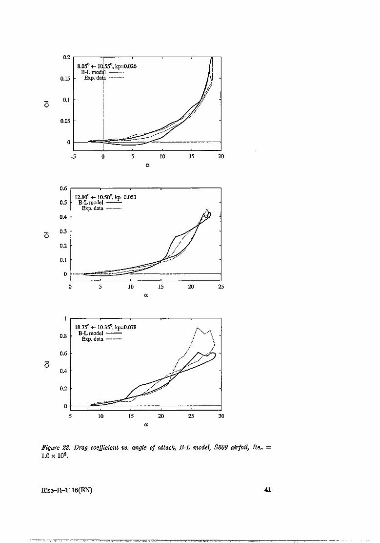
8.05° +- ioj.550, kp=0.026B-L model ---------

Exp. data--------

12.80°+-10.50°, kp=0.053B-L model ---------

Exp. data--------

18.75° +-10.35°, kp=0.078B-L model ---------

Exp. data--------

Figure 23. Drag coefficient vs. angle of attack, B-L model, S809 airfoil, Rec =1.0 x 106.

Ris0-R-1116(EN) 41

Cm

B-L model — Exp. data —

12.80° +- 10.50°, kp=0.053B-L model ---------

Exp. data --------

-0.05 -

-0.1 -

-0.15 -

-0.2 -

-0.25 -

-0.3 -18.75° +- 10.2 B-L model

-0.35 - Exp. data

Figure 24■ Moment coefficient vs. angle of attack, B-L model, S809 airfoil, Rec —1.0 x 106.

42 Ris0-R-1116(EN)

As can be seen from figures 22, 23, and 24, predictions using the Beddoes- Leishman model are relatively good. Overall features are well represented, but at high angles of attack the predictions are not good. The peaks in normal force coefficients are not predicted well, resulting in poor drag and moment predictions. In order to locate the discrepancy the CFD code, EllipSys2D, was run on the third case; a = 18.75° ± 10.35°, kp = 0.078 and the results are displayed below. (Here the experimental data are four consecutive cycles.) The global time step in the unsteady CFD computations is At = 0.002 resulting in 20.000 time steps pr. cycle. (kp = 0.078 corresponds to T = 1 // = c2tt/(kp2U00) = 40.277 non- dimensional sec., where c = 1 and £/«, = 1 ). Since the turbulence intensity in the experimental data is considered relatively high, the computations are made assuming fully turbulent flow. The computations were run for three cycles in order to obtain a periodic solution. The computational time was % 80.000 CPU sec. on an IBM RS6000 3CT.

18.75+-10.35 deg., kp=0.078"EllipSys2D -----. Exp. data ......

B-L model H—

Figure 25. Normal force coefficient vs. angle of attack. B-L model compared with experimental data and CFD computation. The diamonds on the CFD curve cor­responds to streamline plots in figures 28-29. S809 airfoil, Rec = 1.0 x 106.

It is seen that the CFD code captures more features in the hysteresis than the B-L model. Especially at high angles of attack where the CFD code can predict both primary and secondary normal force peaks. At several locations in the CFD hysteresis, streamlines were plotted in order to follow the behavior of the flow. The locations are shown as diamonds on the CFD curve, and the streamline plots are shown in figures 28-29.

Risp-R-l 116 (EN) 43

18.75+-10.35 deg., kp=0.078-EllipSys2D -----

Exp. data ......" B-L model h—

Figure 26. Drag force coefficient vs. angle of attack. B-L model compared with experimental data and CFD computation. The diamonds on the GFD curve cor­responds to streamline plots in figures 28-29. S809 airfoil, Rec = 1.0 x 106.

18.75+-10.35 deg., kp=0.078 EllipSys2D -----Exp. data ......

B-L model

Figure 27. Moment coefficient vs. angle of attack. B-L model compared with exper­imental data and CFD computation. The diamonds on the CFD curve corresponds to streamline plots in figures 28-29. S809 airfoil, Rec = 1.0 x 106.

44 Ris0-R-1116(EN)

Figure 28. Streamline plots from CFD computations of S809 airfoil, correspondingto the diamonds on the CFD curve in figures 25-27.

Ris0-R-1116(EN) 45

Figure 29. Streamline plots from CFD computations of S809 airfoil, corresponding to the diamonds on the CFD curve in figures 25-27.

46 Ris0-R-1116(EN)

The first streamline plot is taken at a = 22.0° on the upstroke. A large trailing edge separation is seen which corresponds well with the slight decrease in normal force coefficient, Cn. Drag force increases rapidly due to the large form drag of the separation bubble, and moment starts to diverge due to the effect of the vortex on the center of pressure. Following the figures downwards it is seen that the separation point moves upstream towards the leading edge, and in plot 4 the separation point has reached the leading edge and a strong leading edge vortex is generated. This vortex is the main reason for the rapid increase in lift since it is stuck to the airfoil for a short period of time. As the vortex grows, it is shed and coincides with the trailing edge vortex. On plot 7 the high lift is caused by bound vortex on the trailing edge. As this detaches from the airfoil the lift decreases rapidly. The very large separation bubble on plot 7 causes a maximum in drag. Drag is also decreasing as the trailing edge vortex is shed. As the large vortex is shed in plot 9, the trailing edge vortex grows rapidly causing a second leading edge separation bubble to be generated. This leads to a second peak in normal force, drag force and moment. At plot 13 the maximum angle of attack is reached, and the downstroke starts, leading to a rapid decrease in normal force and drag force, and an increase in moment.

By investigating the streamline plots it seems clear that the major discrepancy from the B-L model is the leading edge vortex effect. Attempts have been made to model this effect in the B-L model using a comparable procedure, but no general model was obtained.

6.4 NACA 23-010The last unsteady test case is for validating the implementation of arbitrary forcing in the Beddoes-Leishman model. Arbitrary forcing refers to the ability to take into account any prescribed motion, e.g. plunging or lead-lag motion. Unfortunately the available experimental data is very limited, but the measurements of a plunging airfoil by Liiva, ref. [21] were considered appropriate. Tyler and Leishman, ref. [49] used these data for their validation. The experimental data are measurements on a NACA 23-010 airfoil exhibiting plunging motion. Due to the plunging motion an equivalent angle of attack is defined as

, f h\ ,, 360°aeq = arctan 1 — 1 = hkpi (15)

where h is non-dimensional amplitude of the plunging motion with respect to chord. The flow parameters are, Rec = 1.54 x 106, chard = 0.162 m, and M = 0.4 leading to [Zoo = 134 m/s. The three different forced motions are:

• aeq = 0.26° ±3.10°, kpi = 0.129 corresponding to / = 33.9 Hz and h = 0.472.

• aeg = 12.45°±3.14°, kpi = 0.116 corresponding to / = 30.5 Hz and h = 0.419.

• aeq = 14.88°±3.41°, kpi = 0.126 corresponding to / = 33.2 Hz and h = 0.472.

Figure 30 shows computations using the B-L model compared with the experi­mental data.

The low angle of attack case in figure 30 shows good agreement with experi­ments, where both the slope and the openness of the hysteresis is well predicted. For higher angles of attack, where separation is present the largest discrepancy is the misprediction of reattachment during downstroke. This is most pronounced on the Cm curves. The implementation of abitrary forcing is considered acceptable.

EllipSys2D was not applied on this test case, since the Mach number was con­sidered too high.

Ris0-R-1116(EN) 47

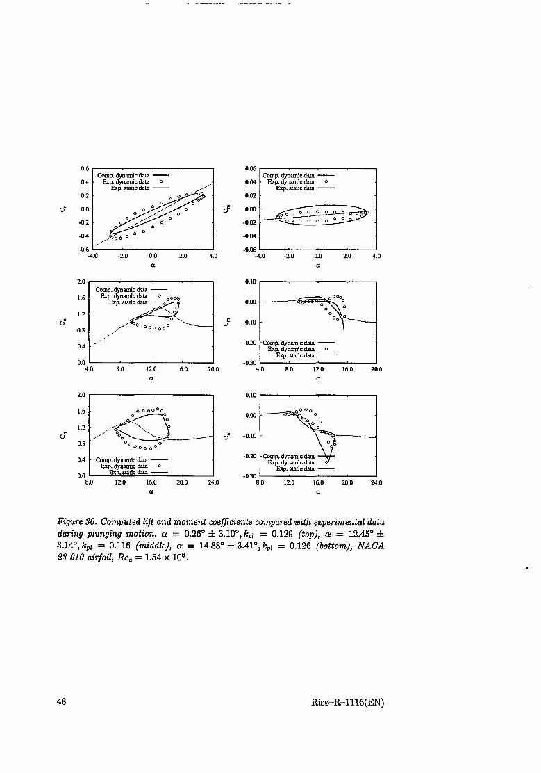
Comp, dynamic data Exp. dynamic data

Exp. static data

Comp, dynamic data Exp. dynamic data

Exp. static data

0.10Comp, dynamic data---------

Exp. dynamic data o OCftExp. static data — 0.00

.../ Oo°oo0o° "-------- .J -0.10 —

-0.20 • Comp, dynamic dataExp. dynamic data °

Exp. static data-0.30

4.0 8.0 12.0 16.0 20.0 4.0 8.0 12.0 16.0 20.0a a

Comp, dynamic data Exp. dynamic data

Exp, static data

Comp, dynamic data Exp. dynamic data

Exp. static data

a a

Figure 30. Computed lift and moment coefficients compared with experimental data during plunging motion, a = 0.26° ± 3.10°, kpi = 0.129 (top), a = 12.45° ± 3.14°, kpi = 0.116 (middle), a = 14.88° ± 3.41°, kpi = 0.126 (bottom), NACA 23-010 airfoil, Rec = 1.54 x 106.

48 Ris0-R-1116(EN)

Discussion

Various subjects have been investigated in the present chapter: The ability of El- lipSys2D to model flow past periodically moving airfoils using both fully turbulent or transitional flow. The comparison between EllipSys2D and the B-L model, and finally the implementation of arbitrary forcing in the B-L model.

The conclusions are as follows: The transition point location does affect sep­aration and correct prediction is important when laminar separation is present. Some numerical problems in the transition model seem to occur during unsteady computations, which could trigger unphysical separation. The B-L model does pre­dict good dynamic stall response unless vortex shedding is present. When vortex shedding is present, a CFD code captures much more details. Finally the plunging motion of a NACA 23-010 airfoil was computed with the B-L mode in order to test the implementation of the arbitrary forcing. Results showed acceptable agreement.

During the present work it was realized that a grid with enough resolution for fixed angle of attack airfoil flows, was not fine enough for dynamic stall cases, since the dynamics of separation and vortex shedding demands more grid points. Despite that, transitional computations predicted separation before fully turbulent computations during upstroke due to laminar separation at the leading edge.

Unfortunately no experimental data were available that completely fulfills the demands when investigating incompressible transitional dynamic stall, and these would be necessary before final conclusions are made.

Ris0-R-1116(EN) 49

Part B:Aeroelastic Modeling

7 Introduction to AeroelasticityAeroelasticity is a discipline where mutual interaction between aerodynamic forces and elastic forces on lifting surfaces is investigated. Of the various areas where aeroelastic phenomena are important parts of the design, airplane design is a ma­jor area, but also helicopters, propellers, turbines, compressors, wind turbines, and wind induced loads on structures (e.g. suspension bridges etc.) are areas where aeroelastic phenomena are present. If these structures where perfectly rigid, aeroe­lastic problems would not exist. But aeroelastic phenomena arise when structural deformations induce additional aerodynamic forces, which may produce additional structural deformations, which again will induce still greater aerodynamic forces. Such interaction may tend to become smaller and smaller until a condition of stable equilibrium is reached, or it may tend to diverge and destroy the structure.

Vortex shedding is one of the key phenomena occurring on flow around a bluff body, causing aeroelastic oscillations. When the bluff body is subjected to a smooth, low-speed flow the most characteristic feature observed in the flow is its separation from the body and the initiation of a more or less agitated wake. The alternating shed vortices induce alternating periodic forces in the direction perpendicular to the motion, and the elastic body moves back and forth. The most famous example of vortex shedding is the von Karman vortex street occurring be­hind a fixed circular cylinder at moderate Reynolds numbers. The frequency at which vortices are shed can be expressed by the Strouhal number St = fsD/Uoo, where fs is the frequency of the natural vortex formulation cycle, D is a represen­tative across-flow dimension of the body, and Uqo is the oncoming uniform flow velocity. The deflection of an elastic body will move at the Strouhal frequency. If the Strouhal frequency approaches the natural frequency (eigenfrequency) of the body, quite large structural deflections may occur.

A second important physical effect which should be mentioned here is the aero­dynamic damping described previously in chapter 5. When energy is extracted from the flow to the body, deflections of the body may increase unless restrained by structural damping.

Basic definitions

Of the various aeroelastic phenomena, the following should be emphasized

• Flutter is a 2 DOF dynamic instability of an elastic body in an airstream occurring at a speed called the flutter speed. The degrees-of-freedom are pitch and flap-wise deflections, respectively. When the speed exceeds this value the aerodynamic forces excites the elastic structure and it begins to vibrate or oscillate. If the overall damping, i.e. aerodynamic as well as structural

50 Ris0-R-1116(EN)

damping, is positive the oscillations damp out. But if the damping is negative the oscillations will increase in size until either the non-linear effects limits the oscillations (LCO) or the structure destroys. The torsional stiffness is the most important stiffness parameter when studying airfoil flutter.

• Stall flutter is the same kind of dynamic instability but is excited by separa­tion and vortex shedding during stall conditions.

• Buffeting is transient vibrations of the structure due to impulses in the flow, i.e. gusts, wake effects, turbulence, etc. The aerodynamic forces are hardly influenced by the motion of the airfoil during buffeting since the vibrations are usually of small amplitude and the frequency has a random distribution.

• Divergence is a static instability of a lifting surface in an air stream occurring at a speed called divergence speed. Since the problem does not depend on time divergence speed can be determined using steady-state aerodynamics and structural equilibrium equations. For the present applications flutter speed is reached before divergence speed.

• Galloping is a large amplitude instability caused by asymmetric effects, i.e. either an asymmetric bluff body (e.g. ice-ladden cable, etc.) subjected to a flow, or a symmetric bluff body subjected to an asymmetric flow (e.g. bundled cables, wake effects, etc.) The frequency of galloping is usually lower than the natural frequency of the structure.

In the present work the aeroelastic phenomena investigated are only classical flut­ter and stall flutter.

Some of the first documented cases of aeroelastic instabilities occurred during World War I, but the aeroelastic discipline was mainly developed during World War II, where the speeds of the airplanes increased and no stiffness criteria from the design were present. The development of the monoplane and large engines urged designers and engineers to take aeroelastic effects into account. The main contributors to the early research in aeroelasticity include Glauert, who inves­tigated potential flow flutter and simple harmonic incompressible motion, and Theodorsen who introduced the typical section two degrees-of-freedom (DOF) airfoil section, and applying his aerodynamic theory for analyzing divergence and flutter problems. Also the work by Garrick should be noticed.

Now the main disciplines within aeroelastic research includes finite element modeling (FEM) coupled with a non-linear aerodynamic model, aeroelastic tailor­ing, transonic aeroelasticity, and the application of CFD coupled with a structural model.

Present work

The main objective of the present work is to couple a three degrees-of-freedom (DOF) structural model to a 2-D CFD code, in order to make aeroelastic compu­tations. The main advantage of this is the much more accurate representation of the non-linear aerodynamic effects. For wind turbine applications, where aeroe­lastic instability mainly occurs when the airfoil operates in the stalled region, the inclusion of non-linear aerodynamics is very important. Therefore the perspective of using CFD for the aerodynamics is well supported.

A second objective is to apply the semi-empirical dynamic stall model by Bed- does and Leishman, ref. [20], on aeroelastic conditions. The approach is to couple the structural model to the non-linear B-L model and integrate through time. This approach includes the non-linear aerodynamic effects included in the B-L model. In this way the behavior of the unstable system can be investigated after flutter

Ris0-R-1116(EN) 51

has occurred, i.e. periodicity (limit cycle oscillations(LCO)), chaos, etc. can be studied. The B-L time integration approach is applied to quickly decide test cases for the unsteady CFD computations, which are much more time consuming.

Finally, by coupling the structural model to the CFD code restrictions of semi- empirical aerodynamic model are avoided leaving only restrictions of the CFD model, and much more detailed information can be determined during the aeroe- lastic computations.

The following chapter, 8, describes the 3 DOF structural model and the equa­tions of motion.

The time integration scheme used for the non-linear unsteady computations is described in section 8.2 together with the solution algorithm for the structural model. The time integration scheme is verified in section 8.3 and various aeroelastic results using the two approaches are presented in chapter 9. The test cases are a2 DOF NACA 0012 airfoil exhibiting both stable and unstable behaviour, and a3 DOF LM 2 airfoil, which in the field is known to exhibit stall induced edge-wise vibrations during certain operational conditions.

Finally an application from the wind turbine area is investigated in section 9.3.

52 Ris0-R-1116(EN)

8 Aeroelastic Model8.1 Structural ModelFor the aeroelastic study a 3 DOF airfoil is chosen, figure 31. The generalized co­ordinates are (x, y, a) in normal, stream-wise and torsional direction, respectively, positive direction as indicated in figure 31. The coordinates in the computational frame of reference are:

(2-ea \ Z %cg I'cg COS Otairfoil X / ®cg ^*cg X2/eo j — I 2leg V*Cg sin Clair foil I ~ I Vcg 1'cg^airfoil I , for O' 1,

&ea ) \ aairfoil ) \ &airfoil )where rcg is the distance the center of gravity, cg lies behind the elastic axis, eo. The elastic axis is in the present study placed in the quarter-chord.

By using Lagrange equations2 the following linear equations of motion are ob­tained

|M]{D}n + [C]{D}„ + pEC]{D}n = {Re3t>„,

where

\K] =

and D are the generalized coordinates.

0 o \ (’ cx 0m ■mrcg , [C] = 0 Cy

—mreg J \. o 0' Kx 0 0 X ( Fx

0 Ky o , {Re=t}n = Fy0 0 Ka J \ M

00

Ca

(16)

Subscript n denotes time, m is the mass, and Ia is the mass moment of inertia about the elastic axis, which is placed at the quarter-chord. mrcg is the static unbalance, Cx, Cy, and Ca3 are structural damping parameters, and Kx,Ky, and Ka4 are spring constants for the three generalized coordinates, respectively. Fx and Fy are the forces in stream-wise and normal direction and M is the moment about the elastic axis. As seen from the mass matrix [M], it is observed that if the elastic axis is placed at the center of gravity, the three equations are uncoupled from a structural point of view, i.e. mrcg = 0. But subjected to a flow the three equations are coupled through the non-linear aerodynamics.

2Lagrange equations: — + d%q.U^ + = 0, T is kinetic energy, U is potentialenergy, g< are generalized coordinates, and Qi are generalized forces.

3Cx,y ~ %TtUj)xtyCxty> Ca — 2Ia&aGa4Kxty ~~ Ka — la^cc

Ris0-R-1116(EN) 53

taoil

incidence

Figure 31. 3 DOF airfoil section, ea is the elastic axis, ac is the aerodynamic center, and eg is the center of gravity.

8.2 Time Integration SchemeThe equations of motion (16) for the non-linear unsteady computations are solved using the Crank-Nicolson method (or the trapezoidal rule). This is an uncondi­tionally stable implicit one-step method, which is second order accurate in time and relates the displacements, velocities, and accelerations as

{P}n+i = {D}n + —({D}„ + (D}n+i),

{D}„+1 = {D}n + ^({D}„ + {D}n+1). (17)

n corresponds to the old time and n 4- 1 is the new time. At is the time step. Rearranging equations (17) gives

{D}n+i = ^({D}n+1-{D}n)-{D}„,

{D}„+1 = ^"({Djn+i - {D}„) - — {D}„ - {D}n. (18)

By combining equations (18) with the equations of motion, equations (16) at time t = n + 1, one finds

[Ke"]{D}n+1 = {Re"}n+i (19)

where the effective stiffness matrix, \Keff], and the effective load vector, {Re^ f }n+i, are, respectively,

= A[m] +A[C] + [K] (20)

and

{Re//Wi = {Re**}n+i + [M](^{D}n + A{D}n + {D>n) (21)

+ [c]{hT>n+^n)This results in a linear system of three equations which are solved using Cramers rule.

54 Ris0-R-1116(EN)

Solution Algorithm

The solution algorithm is as follows:

1 Form mass-, stiffness-, and structural damping matrices.

2 Set initial conditions for displacements and velocities. Use equation (16) to compute initial condition for accelerations.

3 Form effective stiffness matrix, Ke^ from equation (20).

4 Form effective load vector, from equation (21).

5 Solve equation (19) for Dn+i using Cramers rule.

6 Update velocities and accelerations to time t — n + 1 using equations (18)

7 Output if desired or go to 4.

8.3 Verification of Time Integration SchemeIn order to check the accuracy of the integration scheme, integrations are per­formed on conditions where the analytical solution is known. The verification is conducted on a 1 DOF system subjected to a harmonic external force.

The test case under consideration is:

my + cy + ky = F0 sin (cut) (22)

y + 2Cw„y + u\y = — sin(w£)771

wn = yjk/m is the natural frequency of the system, w is the frequency of the external force F0, and ( = c/(2mw„) is the damping ratio. The analytical solution is given by:

= (A3 cos(w<{i) + A4 sin(cvd£)}e Ct,nt

F0/k . ({[i-(y2]2 + (2C^)2}1/2SmV

(23)

+ ut + tan-l 2(w/w» I \ l-(w/w.)=j;

Ag and A4 are determined from the initial values of y and y, here y0 = 0, y = 0, resulting in

Ag = Fojk"{[i-(^)2]2+%)2y/2

sin

C^r)2>1/2 u cos {L}t + tan 1 + A3&n

wd = o;nX/l — C2 is a frequency related to the structural damping. The values of the structural parameters are chosen so they correspond to the order of magnitude used in the aeroelastic study. They are: F„ = 10, m = 1, wn = 10, w = 5, and £ = 0 (i.e. no structural damping), all are non-dimensional. Figure 32 shows the results of the verification.

Ris0-R-1116(EN) 55

bO

0.0001

-4.0

At0.001 0.01 0.1

-3.0 -2.0log At

0.1

0.01

0.001

0.0001

1

le-005-1.0

time (At = 0.01) time (At = 0.05)

Figure 32. Comparison between analytic and computed solution of eq. (23) for different time steps (top left). Numerical error, 0(15), for different time steps (top right). Numerical error, <f>(t), for At = 0.01 (bottom left) and At = 0.05 (bottom right).

The top left figure shows position, y, for the analytical and computed solution of equation (23) for different time steps. The numerical error, 0(15), is here defined as the difference between the analytical and the numerical solution after t = 15 sec., where 4>{t) = yanaiyticai ~ Vnumerical- The error for different time steps is depicted in the top right figure. By plotting the logarithm of the error, 0(15), vs. the logarithm of the time step, (At), the order of the integration scheme can be determined as the slope of the curve. As seen from figure 32 the slope of the curve is 2 leading to the order of the scheme is 2nd order accurate, as expected. The deviation for large time steps is exemplified in the two lower figures. The lower left shows the error at At = 0.01 where the error grows nearly linear. But continuing the computation a beat phenomenon occurs as the error returns to zero, as seen in the lower right figure (At = 0.05). Due to the non-linear growth of the error the last point is not on the linear 2nd order line.

8.4 Coupling with Flow SolverAs mentioned in chapter 5 the computations are performed in a non-inertial frame of reference. The coupling between the structural model and the flow solver is ob­tained by adding the displacements, velocities and accelerations resulting from the structural deflection to the fictitious forces included in the momentum equations. The system of equations are non-linear through the non-linearity of Ci, Ca, and Cm, but by using airfoil characteristics from the previous time step of the flow solution a linearization of the equations is obtained.

For the aeroelastic computations the external forces on the right hand side are the airfoil characteristics from the previous time step only. In this way the order of the time integration scheme can only be of 1st order, but since the airfoil characteristics do not vary much from one time step to the other, in practice the

56 Ris0-R-1116(EN)

«15)

time integration scheme is very close to become 2nd order accurate.

Discussion

As seen from the time integration verifications, the integration scheme is consid­ered as being of appropriate accuracy for the aeroelastic computations. It should be noted here that for unsteady CFD computations the non-dimensional time step is of the order o(10-3) corresponding to a numerical error of o(10-4) assuring that the accuracy of the structural integrations is satisfactory. In the latest version of EllipSys2D, where the dual time stepping algorithm is employed it is now a combi­nation of the structural model and the aerodynamic model that governs the time step. It is important to secure that details of the flow is proper modeled. If high frequency oscillations are present a small time step o(10-3) is necessary to fully resolve the motion and secure 2nd order accuracy of the solution.

Ris0-R-1116(EN) 57

9 Results of Aeroelastic Flows9.1 ValidationFor validating the aeroelastic model a 1 DOF pitching and a 1 DOF flapping case is computed and compared with results using quasi-steady linear aerodynamics. Linear aerodynamics is given by

Cl — 2/T (^incidence: Cm = o2lTCXincidence)where e is the distance between the elastic axis and the aerodynamic center. Using quasi-steady linear aerodynamics an analytic solution is present. Since OCairfoil ~ 01incidence gets Cl = 27f&airfoil 2nd Cm = c2?TO-airfoil

The pmameters for the 1 DOF test cases are: m =64.65 kg/m, Ia = 29.09 kg-m, Uoo = 28.15 m/s, p = 1.293 kg/m3, c = 1 m, and e =-0.15 placing the elastic axis in x/c = 0.4.

1 DOF pitching motion

The natural eigen frequency for the pitching motion is fa — 4.08 Hz, leading to a spring constant of ka = (fa2ir)2Ia = 19117. The initial angle of attack is ao = 6° and the resulting equation of motion is

Iaa + kaa = M = -e2ira-pU%0c

Iaa + (ka + e2npU%0c)a = 0

Solving the equation results in a harmonic oscillation with the frequency

1 I ka + epU^Trc/&new 2-k 2tt Ia

= 4.02Hz.

That is, the frequency of the pitching motion decreases with respect to the natural frequency when subjected to external moment.

1 DOF flapping motion

The natural eigen frequency for the flapping motion is fy = 2.33 Hz, leading to a spring constant of ky = (fy2ir)2m = 13856. The initial deflection is yo — 0.1 c and the equation of motion is

my + kyy = L = -2ir a^pU^c

For flapping motion an equivalent angle of attack is given by

aeq = arctan(-—)Uoo 77-, for a < 1.

This gives:my + irpUooCy + kyy = 0,

which is unconditionally stable with a structural damping coefficient, £ = *p^c- Solving the equation results in a damped oscillation with the frequency

kfyncu)2tt

-hWvy/{1~e)-h zfcy _ .ITpUcoCy.K 2m ‘ ‘ 2.32 Hz.

58 Ris0-R-1116(EN)

Which is only slightly less than the natural frequency. The limiting curve of the damped motion can be expressed by

y(t) = Aq • exp(-5/ync„i)

where Aq is the amplitude at t = 0 and S is the logarithmic decrement defined as

y(t + T) mwyne„

The following Figure 33 shows time series of both 1 DOF test cases using both quasi-steady linear aerodynamics and NS solver. The airfoil employed in the NS solver is the NACA 0015 airfoil. The limiting curve for the damped oscillations is shown in the plot showing the flapping motion.

linear theory--------EllipSys2D---------

linear theory --------i miitSus2p r-T-1

t t

Figure 33. Time series of 1 DOF cases using both linear theory and EllipSys2D NS solver. Pitching case is shown to the left and flapping case is shown to the right.

The time series using linear theory shows excellent agreement with the analytical solution. Using the NS solver a small deviation in both frequency and damping is seen. For the pitching case the frequency is slightly smaller and the motion is slightly damped. For the flapping case the NS computation is less damped and again the frequency is only affected to a small extend. This is caused by unsteady dynamic effects which causes small hysteresis even at these low angles of attack. Figure 34 shows the Cn vs. y/c-curve, where a counter-clockwise rotation indicate a positive aerodynamic damping.

y/c

Figure 34■ C„ vs. y/c hysteresis curve for the flapping 1 DOF case using Ellip- Sys2D NS solver. Counter-clockwise rotation indicate positive aerodynamic damp­ing

Ris0-R-1116(EN) 59

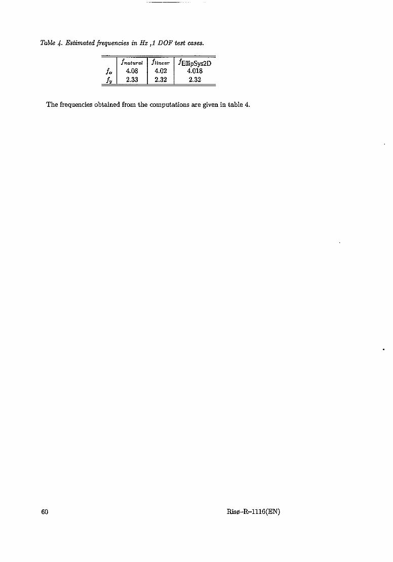
Table 4• Estimated frequencies in Hz ,1 DOF test cases.

/natural flinear /EllipSys2Dfa 4.08 4.02 4.018fy 2.33 2.32 2.32

The frequencies obtained from the computations are given in table 4.

60 Ris0-R-1116(EN)

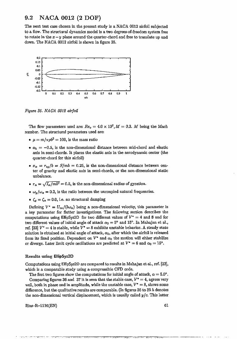
9.2 NACA 0012 (2 DOF)The next test case chosen in the present study is a NACA 0012 airfoil subjected to a flow. The structural dynamics model is a two degrees-of-freedom system free to rotate in the x — y plane around the quarter-chord and free to translate up and down. The NACA 0012 airfoil is shown in figure 35.

0.05 •

Figure 35. NACA 0012 airfoil

The flow parameters used are: Rec = 4.0 x 10s, M = 0.3. M being the Mach number. The structural parameters used are:

• n = m/uptf = 100, is the mass ratio

• Oh = —0.5, is the non-dimensional distance between mid-chord and elastic axis in semi-chords. It places the elastic axis in the aerodynamic center (the quarter-chord for this airfoil)

• xa — Tcg/b = S/mb = 0.25, is the non-dimensional distance between cen­ter of gravity and elastic axis in semi-chords, or the non-dimensional static unbalance.

• ra = y/Ia/mb2 = 0.5, is the non-dimensional radius of gyration.

• u)y/uia = 0.2, is the ratio between the uncoupled natural frequencies.

• Cy = Ca — 0.0, i.e. no structural damping

Defining V* = Z7oo/(&va) being a non-dimensional velocity, this parameter is a key parameter for flutter investigations. The following section describes the computations using EllipSys2D for two different values of V* = 4 and 8 and for two different values of initial angle of attack ao = 5° and 15°. In Mahajan et al., ref. [23] V* = 4 is stable, while V* = 8 exhibits unstable behavior. A steady state solution is obtained at initial angle of attack, ao, after which the airfoil is released from its fixed position. Dependent on V* and ao the motion will either stabilize or diverge. Later limit cycle oscillations are predicted at V* = 6 and ao = 15°.

Results using EllipSys2D

Computations using EllipSys2D are compared to results in Mahajan et al., ref. [23], which is a comparable study using a compressible CFD code.

The first two figures show the computations for initial angle of attack, a = 5.0°. Comparing figures 36 and 37 it is seen that the stable case, V* = 4, agrees very

well, both in phase and in amplitude, while the unstable case, V* = 8, shows some difference, but the qualitative results are comparable. (In figures 36 to 39 h denotes the non-dimensional vertical displacement, which is usually called y/c. This latter

Ris0-R-1116(EN) 61

0.030

0.020

0.010

0.000

-0.010

-0.020

Figure 36. Pitching motion (top left), vertical displacement (top right), Ci (bottom left), and Cm (bottom right) for stable, V* = 4, and unstable, V* = 8, flow conditions. EllipSys2D, ao = 5° = 0.087 rad., NACA 0012, Rec = 4.0 x 106.

-015

-0-015-

t t

Figure 37. Pitching motion (top left), vertical displacement (top right), Q (bottom left), and Cm (bottom right) for stable, V* = 4, and unstable, V* — 8, flow conditions. Mahajan et al., ref. [23], ao = 5° = 0.087 rad., NACA 0012, Rec = 4.0 x 106.

convention is used from figure 40 and further on.) Note that the plunge motion has a smaller dominant frequency than the pitch motion, which is due to the frequency ratio, jj*- = 0.2. A second note is that time has been non-dimensionalized with the freestream velocity and the Mach number, M = 0.3, as in Mahajan et al., ref. [23], to obtain comparable time, and finally, in ref. [23] the vertical displacement has positive direction downwards. This explains the negative displacement, h.

The same conclusions can be drawn for computations with initial angle of at-

62 Ris0-R-1116(EN)

V =8 ---------

V =8 V =8

Figure 38. Pitching motion (top left), vertical displacement (top right), Ci (bottom left), and Gm (bottom right) for stable, V* = 4, and unstable, V* = 8, flow conditions. EllipSys2D, ao = 15° = 0.263 rad., NACA 0012, Rec = 4.0 x 10®.

Figure 39. Pitching motion (top left), vertical displacement (top right), C; (bottom left), and Cm (bottom right) for stable, V* = 4, and unstable, V* = 8, flow conditions. Mahajan et al., ref. [23], ao = 15° = 0.263 rad., NACA 0012, Rec = 4.0 x 10s.

tack, ao = 15°, figures 38 and 39. (Note the change in y — axis in figure 38 to show more information.) The deviations between the two computations can be caused by compressibility effects, different grid topology and time step, difference in implementation, etc. A second note is that the computations from Mahajan et al., ref. [23] is made using the Baldwin-Lomax turbulence model, which is an algebraic turbulence model, while the present computations employ the k—toSST model.

Ris0-R-1116(EN) 63

Limit cycle behavior was observed at V* = 6.0 as shown in figure 40. After a short period of time the motion became periodic in angle of attack, a, while the vertical displacement still showed some non-harmonic behavior. Two phase- plane plots showing angular velocity vs. angle of attack (bottom left) and vertical velocity vs. vertical displacement (bottom right) are shown to demonstrate the periodicity. The two phase-plane plots are plotted after « 500 sec. In Mahajan et al, ref. [23] the flutter speed was determined to V* = 4.75 compared to the present computed value of V* = 6.0.

-30.0 -20.0 -10.0 10.0 20.0 30.0

Figure 40. Limit cycle oscillations (LCO) in pitch (top left) and vertical displace­ments (top right) together with phase-plane plots showing angular velocity vs. angle of attack (bottom left) and vertical velocity vs. vertical displacement (bottom right). V* = 6.0, a0 = 15° = 0.263 rad., EllipSys2D, NACA 0012, Rec = 4.0 x 106.

The total computing time to reach t = 1870 took 320,000 CPU sec. on an IBM RS6000 3CT. The time step for the present computation was At = 0.0028.

Results using Beddoes-Leishman Model

The NACA 0012 test case was also run with the Beddoes-Leishman (B-L) model. For the stable case, V" = 4, ao = 5° the pitch natural frequency is given by fa = Uca/(2irbV*) = 4.48 Hz and the plunge natural frequency is fy = fa ■ 0.2 = 0.90 Hz.

Table 5. Estimated frequencies in Hz, V* = 4, NACA 0012, Rec = 4.0 x 106.

fnatural /EllipSvs2D fs-Lfa 4.48 4.5 5.7fv 0.90 1.1 0.8

The resulting frequencies using both models are summarized in table 5. As seen in subsection 9.1 using linear theory the pitching natural frequency for a ID OF system should decrease while the plunging frequency should remain almost

64 Ris0-R-1116(EN)

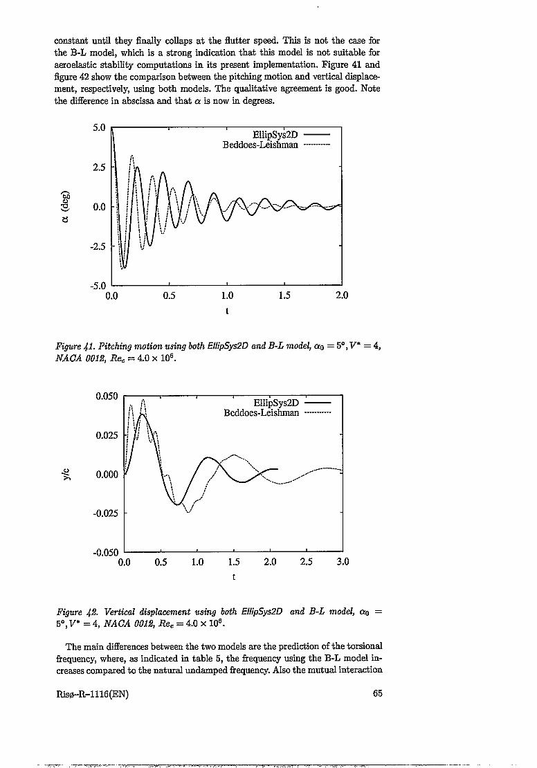
constant until they finally collaps at the flutter speed. This is not the case for the B-L model, which is a strong indication that this model is not suitable for aeroelastic stability computations in its present implementation. Figure 41 and figure 42 show the comparison between the pitching motion and vertical displace­ment, respectively, using both models. The qualitative agreement is good. Note the difference in abscissa and that a is now in degrees.

EllipSys2D B eddoes-Leishman

t

Figure 41- Pitching motion using both EllipSys2D and B-L model, oq = 5°, V* = 4, NAG A 0012, Rec = 4.0 x 106.

EllipSys2DBeddoes-Leishman

-0.025

-0.050

t

Figure 4%- Vertical displacement using both EllipSys2D and B-L model, oto = 5°, V* = 4, NAG A 0012, Rec = 4.0 x 106.

The main differences between the two models are the prediction of the torsional frequency, where, as indicated in table 5, the frequency using the B-L model in­creases compared to the natural undamped frequency. Also the mutual interaction

Ris0-R-1116(EN) 65

between the two degrees of freedom is stronger using the B-L model. After ap­proximately 2 sec. only plunge motion is present. (Note that the x-axis is now non-dimensional time, non-dimensionalized with respect to chord and freestream velocity.)

The unstable test case, (V* = 8), ao = 5°, is shown in figure 43 and figure 44. Here the B-L model fails to reproduce the flutter. The reason for this is probably due to the erroneous prediction of the moment coefficient, leading to an erroneous determination of the aerodynamic damping.

EIlipSys2D B eddoes-Leishman

t

Figure 43. Pitching motion using both EllipSys2D and B-L model, cto = 5°, V* = 8, NAG A 0012, Rec = 4.0 x 106.

EllipSys2DBeddoes-Leishman

t

Figure 44■ Vertical displacement using both Ellip5ys2D and B-L model, ao = 5°, V* = 8, NACA 0012, Rec = 4.0 x 106.

The behavior of the two models for ao = 15° is shown in figures 45 to 48.

66 Ris0-R-1116(EN)

Figures 45 and 46 show the stable case, V* = 4 and «o = 15°, where the B-L model is unstable in pitching motion, which due to the larger coupling between pitch and vertical displacement, also is seen in Figure 46 .

EllipSys2DBeddoes-Leishman

t

Figure 45. Pitching motion using both EllipSys2D and B-L model, «o = 15°, V* = 4, NACA 0012, Rec = 4.0 x 106.

EllipSys2DBeddoes-Leishman

t

Figure 45. Vertical displacement using both EllipSys2D and B-L model, ao = 15°, V* = 4, NACA 0012, Rec = 4.0 x 106.

Ris0-R-1116(EN) 67

For the unstable case ao = 15°, V* = 8 shown in figures 47 and 48 the B-L model shows stable limit cycle oscillations, which is considered unphysical. Again it is probably the misprediction of the moment in the B-L model that causes this behavior.

EllipSys2DB eddoes-Leishman

t

Figure 47. Pitching motion using both EllipSys2D and B-L model, ao = 15°, V* = 8, NACA 0012, Rec = 4.0 x 106.

EllipSys2DBeddoes-Leishman

t

Figure J^8. Vertical displacement using both EllipSys2D and B-L model, ao = 15°, V* = 8, NACA 0012, Rec = 4.0 x 106.

68 Ris0-R-1116(EN)

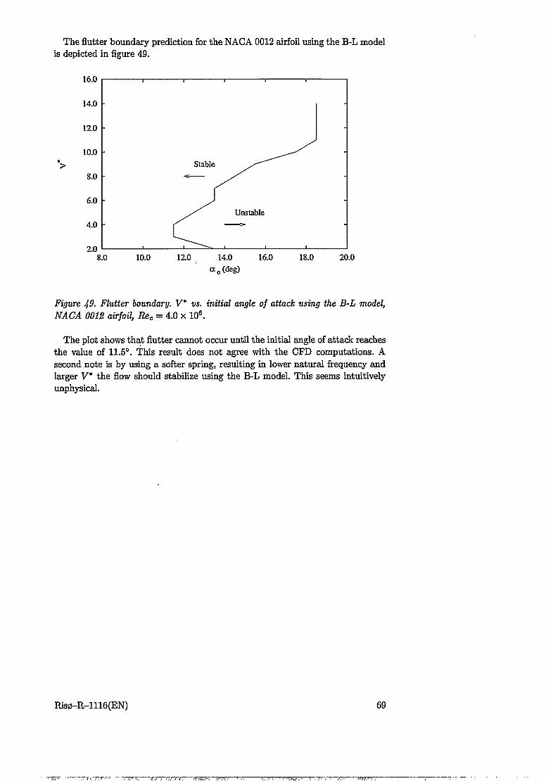
The flutter boundary prediction for the NACA 0012 airfoil using the B-L model is depicted in figure 49.

Stable

Unstable

ctG(deg)

Figure 49. Flutter boundary. V* vs. initial angle of attack using the B-L model, NACA 0012 airfoil, Rec = 4.0 x 106.

The plot shows that flutter cannot occur until the initial angle of attack reaches the value of 11.5°. This result does not agree with the CFD computations. A second note is by using a softer spring, resulting in lower natural frequency and larger V* the flow should stabilize using the B-L model. This seems intuitively unphysical.

Ris0-R-1116(EN) 69

9.3 LM 2 (3 DOF)The second test case studied is the 18 % thick LM 2 wind turbine airfoil. Here the structural dynamics model is a three degrees-of-freedom (DOF) system free to rotate in the x — y plane and free to translate in flap-wise and edge-wise direction. The LM 2 airfoil is shown in figure 50. In wind turbine applications an undesirable

Figure 50. LM 2 airfoil

instability phenomenon referred to as stall induced edge-wise vibrations can occur under certain operational conditions. During stall aerodynamic forces can supply wind turbine blades with energy when they vibrate in a natural mode. Such forces have same direction as the vibration velocity of the blade, and they act as damping forces. This phenomenon is usually denoted negative aerodynamic damping and when it occurs a self-excitation of the structure can occur unless damped through structural damping. This phenomenon is strongly related to flutter described in chapter 7 except that the most unstable degree of freedom is edge-wise motion, or lead-lag motion. Stall induced edge-wise vibrations are known to occur during operational conditions where light stall is observed on the blade. Factors which are known to influence these vibrations are (see Petersen et al, ref. [34]). e.g. static and dynamic airfoil characteristics, overall aerodynamic layout of the blade, i.e. chord length distribution and twist, structural properties of the blade, i.e. structural damping, and properties controlling the direction of vibration, i.e. the principal bending axis. Furthermore properties of the supporting structure, i.e. nacelle and tower has been shown to influence the vibrations as they may either resist or support the vibrations.

In the present section an attempt to predict these edge-wise vibrations as a result of non-linear 2-D aerodynamics is presented. An example taken from Petersen et al. ref. [34] is chosen as test case. i.e. a 40 m diameter wind turbine rotating at a constant speed. An airfoil section at a specific radius from the rotor center is investigated. The aerodynamics in ref. [34], Chapter 2, is based on quasi-steady 2-D aerodynamics, where the influence of lift, drag, lift curve slope, and drag curve slope are investigated. The results show that edge-wise vibrations can occur in the wind speed range 8-25 m/s depending on the direction of vibration, 6. The direction of vibration is caused by the twist of the blade and the structural properties in general. The flap-wise direction is defined as the direction of vibration in the normal direction and the edge-wise direction is the direction of vibration in the chord-wise direction. By rotating the direction of vibration with respect to the elastic axis, the forces are redistributed. Figure 51 shows the influence on translational degrees-of-freedom by rotating the direction of vibration with angle 0.

70 Ris0-R-1116(EN)

Figure 51. Plot showing the influence on translational degrees-of-freedom by rotat­ing the direction of vibration with angle 9.

Here both the CFD code EllipSys2D and the semi-empirical Beddoes-Leishman model is used for the investigation. The main data for the present flow configura­tion are:

• Chord = 1.06 m.

• Radius = 14.0 m.

• Rotational speed, f2 = 3.04 rad/s.

• Direction of vibration angle, 0 = 0° and 9 = —20°. Positive direction is counter-clockwise.

• Mass = 57.0 kg/m -> mass ratio n = 50.

• Moment of inertia = 2.25 kg • m ->• ra = 0.37.

• Flap-wise natural frequency, fy = 1.79 Hz.

• Edge-wise natural frequency, fx = 2.87 Hz.

• Torsional natural frequency, fa = 20.0 Hz.

• Structural damping, £ = 0.0 for all three degrees of freedom.

• Elastic axes at quarter-chord, x/c = 0.25 -f a^ = —0.5.

• Center of gravity at x/c = 0.3 -> rcg = 0.1.

The physical parameters, i.e. mass, moment of inertia, and natural frequencies are measured on an existing blade.

Two wind speeds are considered in the present study, one corresponding to an angle of attack in the attached flow region, and one corresponding to an angle of attack in the separated flow region. They are

• Wind speed = 10 m/s, resulting in Rec = 3.29 x 106 and a = 11.2°.5

• Wind speed = 20 m/s, resulting in Rec = 3.54 x 106 and a = 23.2°.

5Wind speed, W, together with the rotational speed, fir, results in Z7oo(10m/s) = y/Wx+ fi2r* = 43.72 m/s and t/oo(20m/s) = 47.03 m/s. cos a =

W.V-ilT

Ris0-R-1116(EN) 71

Results using EllipSys2D

Figure 52 shows the computations using EllipSys2D with initial angle of attack, «o = 11.2° and direction of vibration, 0 = 0° (top) and —20° (bottom), respec­tively. 9 = —20° is chosen because, as indicated in Petersen et al., ref. [34], this value should cause the system to be more unstable. A second note is that com­pared to the NACA 0012 test case, the structural equilibrium state is placed at ao leading to an oscillation around this value. Time series for the three degrees- of-freedom are shown. The flap and pitch motion are both damped while the edge-wise motion is approximately periodic. It is also observed that the edge-wise amplitude is larger for 9 = —20° compared to 9 = 0°. This is due to the larger contribution from the lift when rotating the axes of vibration. This also leads to a more damped flap and pitch motion.

The frequency of vibration for the edge-wise motion is 2.9 Hz, which is the nat­ural frequency. The frequency of vibration for the flap-wise and pitching motions are 1.8 Hz, which corresponds to the natural frequency of the flap-wise motion, and they are 90° out of phase. When the flap-wise velocity is 0, i.e. either min or max of the position curve, the angle of attack, a = 11.2°. When the airfoil accel­erates upwards a decreases and vice-versa. This means that the change in angle of attack on the left side of figure 52 is the equivalent angle of attack stemming from the flap-wise velocity, aeq = arctan(y/[70O) % y/Uoo■ The high frequency "noise” on the pitching motion is the change in geometric angle of attack of the airfoil at the pitching natural frequency, fa = 20 Hz.

flap ---------edge------

0.75 :

Figure 52. Time series for LM 2 airfoil using EllipSys2D, ao = 11.2°, Rec = 3.29 x 106, direction of vibration 9 = 0°(top) and —200(bottom), respectively.

72 Ris0-R-1116(EN)

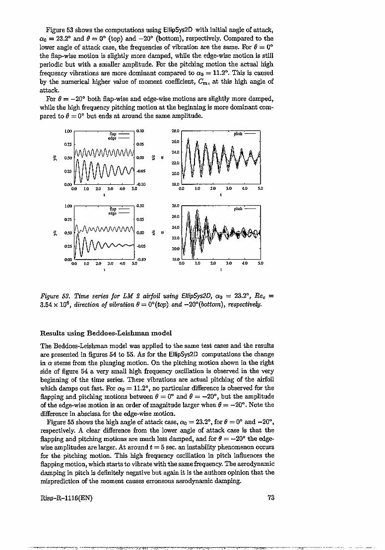
Figure 53 shows the computations using EllipSys2D with initial angle of attack, ao = 23.2° and 0 = 0° (top) and —20° (bottom), respectively. Compared to the lower angle of attack case, the frequencies of vibration are the same. For 0 = 0° the flap-wise motion is slightly more damped, while the edge-wise motion is still periodic but with a smaller amplitude. For the pitching motion the actual high frequency vibrations are more dominant compared to ao = 11.2°. This is caused by the numerical higher value of moment coefficient, Cm, at this high angle of attack.

For 0 = —20° both flap-wise and edge-wise motions are slightly more damped, while the high frequency pitching motion at the beginning is more dominant com­pared to 0 = 0° but ends at around the same amplitude.

1.00flap ■

edge--------

0.10

0.75 0.05

0.50(WWWM/V#

0.00

0.25 -Oj05

0.00I V v v

-0.100.0 1.0 2.0 3.0 4.0 5.0

t

flap —

' 0.0 1.0 2.0 3.0 4.0 5.0

t

Figure 53. Time series for LM 2 airfoil using EllipSys2D, ao = 23.2°, Rec = 3.54 x 106, direction of vibration 6 = 0°(top) and —20°(bottom), respectively.

Results using Beddoes-Leishman model

The Beddoes-Leishman model was applied to the same test cases and the results are presented in figures 54 to 55. As for the EllipSys2D computations the change in a stems from the plunging motion. On the pitching motion shown in the right side of figure 54 a very small high frequency oscillation is observed in the very beginning of the time series. These vibrations are actual pitching of the airfoil which damps out fast. For ao = 11.2°, no particular difference is observed for the flapping and pitching motions between 0 = 0° and 0 = —20°, but the amplitude of the edge-wise motion is an order of magnitude larger when 0 = —20°. Note the difference in abscissa for the edge-wise motion.

Figure 55 shows the high angle of attack case, ao = 23.2°, for 0 = 0° and —20°, respectively. A clear difference from the lower angle of attack case is that the flapping and pitching motions are much less damped, and for 0 = —20° the edge­wise amplitudes are larger. At around t = 5 sec. an instability phenomenon occurs for the pitching motion. This high frequency oscillation in pitch influences the flapping motion, which starts to vibrate with the same frequency. The aerodynamic damping in pitch is definitely negative but again it is the authors opinion that the misprediction of the moment causes erroneous aerodynamic damping.

Ris0-R-1116(EN) 73

0.010flap ---------

0.005

0.000

-0.0Q5

-0.010

flap ---------edge --------

0.0 1.0 2.0 3.0 4.0 5.0l

6.0 1----------------- '----------------- '----------------- '----------------- '-----------------

0.0 1.0 2.0 3.0 4.0 5.0t

pilch ---------

Figure 54• Time series for LM 2 airfoil using B-L model, direction of vibration, 6 = 0°(top) and —20°(bottom), respectively. = 11.2°, Rec = 3.29 x 106.

Figure 55. Time series for LM 2 airfoil using B-L model, direction of vibration,6 = 0°(top) and —20°(bottom), respectively. <%o = 23.2°, Rec = 3.54 x 106.

74 Ris0-R-1116(EN)

Discussion

Aeroelastic computations have been carried out using EllipSys2D coupled to a structural dynamics model. The model has been validated against two 1 DOF cases and was applied on a 2 DOF NACA 0012 airfoil case. Comparison with a numerical study from the literature was carried out using the NS solver, EIIipSys2D, and results showed good agreement. The Beddoes-Leishman model was applied on the same test case, but only the stable cases were correctly predicted. Both models were applied to a 3 DOF LM 2 airfoil to investigate stall induced edge­wise vibrations. EllipSys2D and the B-L model were in very good agreement when predicting the aeroelastic response, where stable solutions were expected. The only significant difference was the larger pitching response predicted by EllipSys2D.

At the high angle of attack case EllipSys2D predicts more damping and again the pitching motion is more dominant. But by rotating the direction of vibration in the clockwise direction the pitching motion increases in amplitude with both models, and for the B-L model it actually becomes unstable.

The overall conclusion on the B-L model is that the moment is not properly predicted, resulting in an erroneous aerodynamic damping, which is a key factor for flutter prediction. For the stable solution, i.e. low a, the aerodynamic damping plays a minor role and the response is predicted acceptably well. When instability according to EllipSys2D is present the aerodynamic damping play a greater role and because of it’s misprediction, non-physical response is computed using the B- L model. For proper use of the B-L model in aeroelastic analysis, a better model for the moment coefficient is needed.

At the very end of the present project it was found more appropriate to define the direction of vibration with respect to the airfoil and not as done in the present work, with respect to inflow. This will better represent real physics and might be the reason for not being able to predict stall induced edge-wise vibrations.

Ris0-R-1116(EN) 75

10 ConclusionsThe present work has described numerical investigation of two-dimensional un­steady airfoil flows with application to aeroelastic stability.

The objectives of the work were twofold. First a transition prediction model based on the en method was developed. A laminar integral boundary layer for­mulation based on dissipation closure were implemented and coupled to a Navier- Stokes solver, EllipSys2D, and the resulting boundary layer parameters, i.e. velocity at the edge of the boundary layer, displacement thickness, momentum thickness, and kinetic energy thickness, were used as input to an instability database. The database is built of a discrete set of solutions to the Orr-Sommerfeld equation, and by using laminar boundary layer parameters as input, stability information can be determined by interpolation. The laminar integral boundary layer formu­lation was solved by a coupled direct/inverse Newton-Raphson method in order to get boundary layer parameters well into the separated region. The transition model was validated on a flat plate flow. Quasi-static computations were con­ducted on various airfoils under static conditions. Transitional computations with the developed transition prediction model were compared with fully turbulent computations and transitional computations using an empirical transition model, the Michel Criterion, as well as experimental data. Results showed clear improve­ments in drag predictions using transition models, but also the lift characteristics showed a slightly better prediction using transition models. The difference in pre­diction between the two models is small, but the en model showed more stable solutions compared to the Michel Criterion.

In order to investigate unsteady airfoil flows with respect to dynamic stall, a semi-empirical dynamic stall model, the Beddoes-Leishman (B-L) model, was applied for comparison with the Navier-Stokes solver. The present version of the B-L model was originally implemented by Pierce, ref. [35] but additions were made during the present work in order to take arbitrary forcing into account, i.e. plunging and lead-lag motion.

Dynamic stall computations were carried out on the NACA 0015 and the RIS0- 1 airfoils in order to investigate the influence of transition on dynamic stall. Un­fortunately the experimental test cases were not very suitable for incompressible transition modeling. But overall conclusions are that, as for fixed angle of attack flows, drag is better predicted using a transition model. A second major conclu­sion is the importance of proper grid resolution. During the process of computing dynamic stall it was realized that a fine enough grid for fixed angle of attack flows, was not fine enough for dynamic stall computations, since the dynamics of separation and vortex shedding demands more grid points. Despite that, tran­sitional computations predicted separation before fully turbulent computations during upstroke due to laminar separation at the leading edge.

The RIS0-1 and S809 airfoils were also investigated using the B-L model. It showed good lift and drag predictions as long as leading edge separation was not present. The moment predictions failed to reproduce the experimental data when separation was present. The computations using the Navier-Stokes solver showed better qualitative agreement especially when leading edge separation was present. The ability to get detailed information on the overall unsteady flow field revealed useful information for further development of the B-L model. Finally the plunging motion of a NACA 23-010 airfoil was computed with the B-L model in order to test the implementation of the arbitrary forcing. Results showed acceptable agreement.

In the second part of the work the aerodynamic models were coupled to a simple three degrees-of-freedom (DOF) structural dynamics model to make aeroe-

76 Ris0-R-1116(EN)

lastic investigations. The structural dynamics model was developed and the time integration algorithm was verified. Two test cases were investigated. The first was a 2 DOF NACA 0012 airfoil subjected to an air flow. The airfoil was pitched up­wards to an initial angle of attack and then released. Dependent on the natural frequency of the pitch spring the airfoil motion was either damped or excited. Computations were done using both EIiipSys2D and the B-L model and compared to comparable computations from the literature. Good agreement was obtained for stable conditions at low initial angle of attack, but for the unstable conditions only EllipSys2D predicted correct aeroelastic response. The B-L model was not able to predict the same unstable conditions, which was interpreted as being a poor prediction of moment resulting in erroneous aerodynamic damping.

The second test case was the investigation of a 3 DOF wind turbine airfoil which is known to experience stall induced edge-wise vibrations during certain operational conditions. An attempt to model this was done. Two wind speeds cor­responding to two angles of attack; one in the attached region and one in the stalled region. Also the effect of rotating the direction of vibration was investigated. Both aerodynamic models agreed well on the low angle of attack case where flap-wise vibrations damp out and the main contribution to the pitching motion was due to the equivalent angle of attack stemming from the plunging motion. Edge-wise vibrations were small but more or less periodic. The B-L model did predict more aerodynamic damping, though. By rotating the direction of vibration the force distribution was changed causing larger edge-wise amplitude and more damped flap-wise motion. The frequencies of the aeroelastic response corresponded well with the natural frequencies of the structural model.

At high angles of attack both models predicted more dominant pitching mo­tion and by rotating the direction of vibration EIIipSys2D predicts more flap-wise damping, while the pitching motion at the beginning increases but ends at the same amplitude as for not rotating the direction of vibration. The B-L model shows less aerodynamic damping compared to the low angle of attack case and by rotating the direction of vibration the edge-wise amplitudes becomes larger. After a short while an instability phenomenon occurs for the pitching motion. This high frequency oscillation in pitch influences the flapping motion, which starts to vibrate with the same frequency. The aerodynamic damping in pitch is definitely negative but again it is the authors opinion that the misprediction of the moment causes erroneous aerodynamic damping.

The direction of vibration was in the present work defined with respect to the inflow. It would have been more appropriate to define it with respect to the airfoil. This would better represent real physics, and might be a reason for not being able to predict stall induced edge-wise vibrations.

10.1 Recommendations for Further ResearchThe present work has described contributions to the field of numerical aerody­namics and aeroelasticity. For both disciplines it is of major importance to obtain proper experimental data for validating and testing. This includes low turbulence intensity wind tunnel test of smooth airfoils at low Mach numbers. Both static and dynamic (Pitching, plunging, and lead-lag oscillations) data are necessary, including aeroelastic test cases with one, two, or three degrees-of-freedom.

For unsteady CFD computations it is of major importance to perform grid refinement studies to secure grid insensitive solutions.

The Beddoes-Leishman model has to be extended to better predict moment coefficients and vortex shedding for proper prediction of aerodynamic damping. The problem is, if it is possible to include these very complex dynamic phenomena in an indicia! response formulation comparable to the original formulation.

Ris0-R-1116(EN) 77

In the case of aeroelastic modeling it would have been more appropriate to compare the two different aerodynamic models with simpler aeroelastic configura­tions, such as e.g. classical flutter, and also to test the structural dynamics model together with linear aerodynamic theory. Furthermore it would be more appropri­ate to define the direction of vibration with respect to the airfoil and not, as in the present work, with respect to inflow. Using the other definition would better represent real physics.

The effects of including structural damping, non-linear springs, and non-linear generalized coordinates is an obvious extension to the structural dynamics model

The major future task is to extend the models to three-dimensional flows. In the case of transition modeling using the proposed model, the solution of the integral boundary layer equations and defining laminar boundary layer parameters must be the major task. By extending the aeroelastic model to 3-D, the inclusion of an extra field of research is necessary: Adaptive grid generation. As the different airfoil sections on a wing deflects, the wing deforms and a new grid has to be generated at each time step. This will increase the computing time considerably compared to pure 3-D aerodynamic computations. Also the structural dynamics model will have to be further developed to include more degrees-of-freedom.

78 Ris0-R-1116(EN)

References[1] Abbott, I. H., and von Doenhoeff, A. E. Theory of Wing Sections.

Dover Publications, Inc., New York, 1959.

[2] Althaus, D., and Wortmann, F. X. Stuttgarter Profilkatalog 1. Tech, rep., F. Wieweg, Braunschweig, 1981.

[3] Arnal, D. Boundary Layer Transition: Predictions based on Linear Theory. Tech, rep., AGARD, 1994. AGARD-R-793.

[4] Bisplinghoff, R. L., Ashley, H., and Halfman, R. L. Aeroelasticity. Dover Publications, Inc., 1955.

[5] Carr, L. W. Progress in analysis and Prediction of Dynamic Stall. J. Aircraft 25,1 (1988), 6-17.

[6] Cebeci, T. Essential Ingridients of a Method for Low Reynolds-Number Airfoils. AIAA J. 27, 12 (1988).

[7] CHEN, K. K., AND Thyson, N. A. Extension of Emmons Spot Theory to Flows on Blunt Bodies. AIAA J. 9, 5 (1971), 821-825.

[8] Cowley, S. J., AND Wu, X. Asymptotic Approaches to Transition Mod­elling. Tech, rep., AGARD, 1994. AGARD-R-793.

[9] Dini, P., Selig, M. S., and Maughmer, M. D. Simplified Linear Stability Transition Prediction Method for Separated Boundary Layers. AIAA J. SO, 8 (1992), 1953-1961.

[10] Drela, M., and Giles, M. B. Viscous-Inviscid Analysis of Transonic and Low Reynolds Number Airfoils. AIAA J. 25, 10 (1986).

[11] Ekaterinaris, J. A., Chandrasekhara, M. S., and Platzer, M. F. Analysis of Low Reynolds Number Airfoil Flows. Journal of Aircraft (1995), 625-630.

[12] Ekaterinaris, J. A., and Platzer, M. F. Computational Prediction of Airfoil Dynamic Stall. Prog. Aerospace Sci. 33 (1998), 759-846.

[13] Ericsson, L. E., and Reding, J. P. Fluid Mechanics of Dynamic Stall Part I. Unsteady Flow Concepts. J. of Fluids and Structures 2 (1988), 1—33.

[14] Fuglsang, P., Antoniou, I., Bak, C., and Madsen, H. A. Wind Tunnel Test of the RIS0-1 Airfoil. Tech, rep., Risp National Laboratory, Roskilde, Denmark, May 1998.

[15] Galbraith, R. A. M., Gracey, M. W., and Leith, E. Summary of pressure data for thirteen aerofoils on the University of Glasgow’s aerofoil database. Tech, rep., University of Glasgow, 1992.

[16] Gangwani, S. T. Synthesized unsteady airfoil data method for prediction of dynamic stall and unsteady airloads. Tech, rep., 1983. NASA CR 3672.

[17] HERBERT, T. Parabolized Stability Equations. Tech, rep., AGARD, 1994. AGARD-R-793.

[18] ISSA, R. Solution of the Implicitly Discretised Fluid Flow Equations by Operator-Splitting. J. Comp. Phys. 62 (1985), 40-65.

[19] Jones, W. P., and Launder, B. E. The Prediction of Laminarization with a Two-Equation Model of Turbulence. Int. J. of Heat and Mass Transfer 15 (1972), 301-314.

Ris0-R-1116(EN) 79

[20] Leishman, J. G., and Beddoes, T. S. A Semi-Empirical Model for Dy­namic Stall. J. of the American Helicopter Society (1986).

[21] Liiva, J., Davenport, F. J., Gray, L., and Walton, I. C. Two- Dimensional Tests of Airfoils Oscillating Near Stall. Tech, rep., 1968.

[22] Madsen, H. A. Design of a 20 kW - 12.6 m Stall Regulated Rotor. Tech, rep., Ris0 National Laboratory, Roskilde, Denmark, 1994.

[23] Mahajan, A. J., Kaza, K. R. V., and Dowell, E. H. Semi-Empirical Model for Prediction of Unsteady Forces on an Airfoil with application to Flutter. J. of Fluids and Structures 7 (1993), 87-103.

[24] McCroskey, W. J. The Phenomenon of Dynamic Stall. Tech, rep., 1981. NASA T.M. 81264.

[25] McCroskey, W. J. Unsteady Airfoils. Ann. Rev. Fluid Mech. (1982).

[26] Mehta, U., Chang, K. C., and Cebeci, T. Relative Advantages of Thin- Layer Navier-Stokes and Interactive Boundary-Layer Procedures. Tech, rep., NASA, 1985. Technical Memorandum.

[27] Menter, F. R. Zonal Two Equation k — u> Turbulence Models for Aerody­namic Flows. AIAA Paper 93-2906.

[28] Michel, R. Etude de la Transition sur les Profiles d’Aile;Etablissement d’un Critere de Determination de Point de Transition et Calcul de la Trainee de Profile Incompressible. Tech, rep., ONERA, 1951. Report 1/1578A.

[29] Michelsen, J. A. Basis3D - a Platform for Development of Multiblock PDE Solvers. Tech, rep., Technical University of Denmark, 1992. AFM 92-05.

[30] Michelsen, J. A. Block structured Multigrid solution of 2D and 3D elliptic PDE’s. Tech, rep., Technical University of Denmark, 1994. AFM 94^06.

[31] Olesen, N. A. Laminar/Turbulent Omslagsmodel for Graense- lagsstrgmninger. Master’s thesis, Danish Technical University, 1994. AFM- EP 94-02.

[32] Patankar, S. V. Numerical Heat Transfer and Fluid Flow. Hemisphere Publishing Corporation, 1980.

[33] Petersen, E. D. Graenselagsstabilitet. Master’s thesis, Danish Technical University, 1991. AFM-EP 91-01.

[34] Petersen, J. T., Madsen, H. A., Bjork, A., Enevoldsen, P., 0ye, S., Ganander, H., and Winkelaar, D. Prediction of Dynamic Loads and Induced Vibrations in Stall. Tech, rep., Ris0 National Laboratory, Roskilde, Denmark, May 1998.

[35] Pierce, K. G. Wind Turbine Load Prediction using the Beddoes-Leishman Model for Unsteady Aerodynamics and Dynamic Stall. Master’s thesis, The University of Utah Graduate School, August 1996.

[36] Ramsay, R. R., Hoffman, M. J., and Gregorek, G. M. Effects of Grit Roughness and Pitch Oscillations on the S809 Airfoil. Tech, rep., National Renewable Energy Laboratory, Colorado, USA, 1995.

[37] Rasmussen, F., Petersen, J. T., and Madsen, H. A. Response Predic­tion by Application of a New Dynamic Stall Model. In 1996 European Union Wind Energy Conference (1996), EWEC, pp. 838-841.

80 Ris0-R-1116(EN)

[38] Rumsey, C. L., Saneteik, M. D., Biedron, R., Melson, N. D., and

Parlette, E. Efficiency and Accuracy of Time-Accurate Turbulent Navier- Stokes Computations. AIAA Paper 95-1835.

[39] Schlichting, H. Boundary-Layer Theory. McGraw-Hill, Inc., 1987.

[40] Smith, A. Transition, Pressure Gradient, and Stability Theory. In Proceed­ings of the IX International Congress of Applied Mechanics (1956), vol. 4, pp. 234-244.

[41] Somers, D. M. Design and Experimental Results for the S809 Airfoil. Tech, rep., National Renewable Energy Laboratory, Colorado, USA, January 1997.

[42] Sorensen, N. N. General Purpose Flow Solver Applied to Flow over Hills. Tech, rep., Risp National Laboratory, Roskilde, Denmark, June 1995. Ph.D. Thesis, Ris0-R-827(EN).

[43] Sorensen, N. N. k-w Turbulence Models Implementation and Testing. Tech, rep., Ris0-R-864(EN), 1995.

[44] Sorensen, N. N. HypGrid2D - a 2-D Mesh Generator. Tech, rep., Ris0

National Laboratory, Roskilde, Denmark, March 1998.

[45] Stock, H., and Degenhart, E. A simplified en method for transition prediction in two-dimensional, incompressible boundary layers. Z. Flugwiss. Weltraumforsch. 13 (1989).

[46] Timmer, W. A. WECS Blade Airfoils - The NACA 63-4XX Series. European Community Wind Energy Conference.

[47] Timmer, W. A., and van Rooy, R. P. J. O. M. Wind Tunnel Results for a 25% Thick Wind Turbine Blade Airfoil. European Community Wind Energy Conference.

[48] Tran, C. T., and Petot, D. Semi-empirical Model for the Dynamic Stall of Airfoils in view of the Application to the Calculation of Responses of a Helicopter Blade in Forward Flight. Vertica 5 (1981), 35-53.

[49] Tyler, J. C., and Leishman, J. G. An Analysis of Pitching and Plunge Effects on Unsteady Airfoil Behavior. J. of the American Helicopter Society 37, 3 (July 1992), 69-82.

[50] VAN INGEN, J. A Suggested Semi-empirical Method for the Calculation of the Boundary-Layer Region. Tech, rep., Delft,Holland, 1956. Rept. No. VTH71, VTH74.

[51] White, F. M. Viscous Fluid Flow, 2 ed. McGraw-Hill Inc., 1991.

[52] Wilcox, D. C. Turbulence Modeling for CFD. DCW Industries, Inc., 1993.

Ris0-R-ll 16 (EN) 81

A Discretization of Boundary Layer EquationsThe boundary layer equations (8) and (9) are discretized using a 2. order central differencing scheme.

Direct solution procedure

For the direct solution procedure, where the freestream velocity, ue, is determined by the N-S solver, the two remaining parameters, H and 0 can be computed solving equations (8) and (9) directly using a Newton-Raphson procedure. This results in the following discretized equations.

h

h

0j ~ 0i-l , (n , Hi + Hi-1 ^ 0{ + 0j-l Uei - %g;_i CfV+ —2---- ) 6-6., “ T'-l - 0

0, + 0,-i dH* Hi — Hi-1 / Hi 4- Hi-1 \ 6j + 0j-i uei — uei_t2 dH 6 — 6-1 1-2 V, 2 )uei+ue{_j 6 —6-1

2C^ _!%_!= 0 (A.1)

ff*, and 2Cx> are given by relationships (10), (11), and (12) respectively. The chain rule is used for

where

dH*8H

dH*dH

= 0.076 1 -

= 0.040 1 -

dH* dH* dH ~df~~dHdC

16 '(iM,--1)2 J '

____«____)(Hi+fi~1)2 ) ’

H< 4

if >4.

For the direct solution procedure the matrix equation is given by

(A.2)

(A.3)

a/i dh a/i e/i6Bi—i ia/2 a/2 a/2 a/2ay*—i a/fi—i a^i a/fi

/ 50, -1 \ 5Hi-i

50i\ SHi )

(A.4)

Since the parameters at the previous boundary layer station is already computed resulting in <50j_i and 5if,-_i = 0, equation (A.4) is reduced to the following very simple system of equations.

§±La& WLdBi dHi

where

9fi _ 1 Hj + Hj-A uei -uei_x 1

90i 6 — 6-i x 2 / uei + uei_i 6 — 6-idfi _ 1 9j + 0,-i uei—uei_t

2 Uei + 6 — 6-1 dHi ’

(A.5)

’

82 Ris0-R-1116(EN)

3/2

ddi18H* Hi — Hi-i2 8H 6-6-1

-T

and

df2 6 + 6-1 (dH*8Hi 2 [dH

3%-

1 Hi — Hj-i)3

+ 6+ft-l / g* 3-ff*A gj + gj-i\\««+«„_, 6-6-1 X 2 Sir ^ 2 ))

_82Co + asrcL ,a£ as, 8J? 2 '-isifi

This system of equations is a simple 2x2 system and is solved using rule.

Cramers

Inverse solution procedure

As the flow approaches separation the integral boundary layer equations are solved inversely with 6 and ue as the independent variables. The skin friction, Cf can be determined using the N-S solver and from relationship (11), the shape factor H is computed. The discretized equations, (A.l), are equal to those for the direct procedure. For the inverse solution procedure the matrix equation is given by

/ &El «&-I 86 i 8ue;I 8Sx 8 Si\ 8$i 8uc{

(A.6)

wheredfi _ 1 . A, . Hj + Hi-1 \ uei - ue,_i 136 6 — 6-i X 2 ) uei + 6 — 6-1 ’

dfi _ /X Hj + Hj-i \ 6ei + dej-i 2ue;_i duei V 2 / 6 — 6-1 (uei +Uei-i)2’

dfi _ ue; - uei_x 1 f Hi + Hi-i \ 1 dH* Hi — Hi-i 82Cp80i ~ 6-6-1 MX 2 ) + 2 8H 6-6-1 36 ’

anddfi _ 6j + 6-1 m 1 A _ + -Hj-i \ 2ue._t______82Cp8ue. ~ 6-6-1 i-= X 2 / (uei +ue;_i)2 3ues

The derivatives of and 2Cp with respect to 6, H and ue are rather lengthy but straightforward.

Ris0-R-1116(EN) 83

B Beddoes-Leishman Dynamic Stall ModelThe following sections describe the three sub-systems of the Beddoes-Leishman model, i.e. the attached flow region, the separated flow region, and the dynamic stall region. Also the modeling of the unsteady drag force is described.

B.l Attached FlowIn general the indicial lift and quarter-chord pitching moment coefficients for a step change in angle of attack, a, and pitch rate, q, can be written as (Bisplinhoff et ffi., ref. [4])

CnQ = CrtTa + C%Q = + "jg"0a^ “ 08'7)

Cmcc = Cmoc + Cmo — -----~p(t><a[Xac ~ 0-25]^ a

CNg - C*Nq + Cffg : ~ Q

Cmq = cifq + C%fg ----- - 8/?^m) q

where <j> is the indicial response functions. M is the Mach number, 0 is the Prandtl- Glauert compressibility factor, 0 = Vl — M2, and xac is the aerodynamic center. The superscripts I and C refer to the components of impulsive and circulatory loading, respectively. Subscripts N and M refer to normal force and pitching moment, respectively. In practice the linearized value of the steady lift curve slope 2tt//? is replaced by the measured steady state normal force curve slope CUa. The indicial response functions are approximated empirically in terms of exponential functions. (Leishmem and Beddoes, ref. [20].)

0a = «*P ((B.8)

<j>a = 1 - Ai exp(-bi02S) - A2 exp(~b202S)

= esp(^)4>q = 0a = 4>C

^ = Asexp(si^)+'44exp(^)= “p(^)

<!>% = 1 - A5 exp(-65/32S)

The constEmts Aj and bj are empirically determined constants and Tj are empiri­cally determined time constants dependent on Mach number. 5 = 2Uoat/c is the non-dimensional distance traveled by the airfoil in semi-chords. These response

84 Ris0-R-1116(EN)

functions are discretized using the previously mentioned method using Duhamel’s integral. In this way the cumulative effect to an arbitrary time history of angle of attack is constructed.

The following sections describe the discretization of the various circulatory and impulsive components of normal force and moment, respectively.

Normal forceFor unsteady flow, the circulatory component of the normal force coefficient can be written as

Cn„ = CNa<f>caE = CNaUqo

where n is the current sample, a# is an effective angle of attack, wE is the effective downwash at the 3/4-chord, and [7<x> is the freestream velocity. To compare pitch and plunge motion an equivalent angle of attack is defined for plunging as (Tyler and Leishman, ref. [49])

aeq = arctan

where y is the plunge velocity. For an airfoil undergoing arbitrary pitch a and plunge y about the 1/4-chord, the instantaneous quasi-steady down wash at the 3/4-chord is given by

_yUc8=6'

w = alloo + Q + y,

where Q = —qUco/2 and q = ac/U^ is the non-dimensional pitch rate. (Q is simply dimensionalized pitch rate with semi-chord, i.e. Q = d|). The effective down wash is given by

wE = Etfoo. Aan - X& - y„(1) + Sa„AC/00„ - X™ - Fn(2) (B.9)

+ sa Qn - x&3) - y„(3) + sa hn - x44) - y„(4).Xn^ and Yn^ are deficiency functions, which represents the deficiency in the quasi-steady values due to the presence of unsteady shed wakes. They are given by

X& = expi-hfAS) +A1 A« exp

yn0) = Yn-i exp(-62/S2AS) + A2A(j) exp ^ ,

where A^ terms are the corresponding change of angle of attack, velocity, pitch rate, and plunge, respectively, from one time step to the next given by

AW = UoonAan and A(2) = a„A[7COn (B.10)

A^) = A qn and A^) = A yn.

In the original implementation, Pierce, ref. [35] only the angle of attack term Qf1) and pitch rate term Q(3) was included.The impulsive part of the normal force due to a step change in angle of attack is given by

Gk4KaTi (Aan

M \ At

Bis0-R-1116(EN) 85

In this case the deficiency function, D„, is given by

Dn = Dn_! exp ( ~At \ + (Aan ~ Aa'

\KaTj) + V At

Ka is a factor associated with the non-cirdilatory time constant and Tj = c/o is a time constant governing the decay of the loads due to the propagation of pressure disturbances, c is the chord and o is the speed of sound.The impulsive part of the normal force due to a step change in pitch rate is given by

where

—KgTi Z A qn M \ At

f Agn - Ag, \ At

Again AT, is a factor associated with the non-circulatory time constant. No impul­sive part due to Z/qo and h is present.The total normal force is given by

cN=c$+clJaNT + CqNnMoment

The impulsive part of the moment terms due to a step change in angle of attack is in the present work modeled using

CaMr —

The impulsive part of the moment terms due to a step change in pitch rate is given by

-7KqMTi Z Agn _ „ 12 M \ At

DIIQn

( —At A Z Agn — Agn_! \K*mTi ) + { At

The circulatory part of the moment terms is given by

Cm„ — Cm0 + (0.25 — xac)Cxn----^-(9n - .

Here Cm0 is the zero lift moment coefficient. In the present work the second term is neglected since the aerodynamic center is usually less than 0.02 chord lengths from the quarter chord. The deficiency function is given by

45) = 4-i exp(—65/?2AS) + A5Agn exp .

The total moment is given by

Cm„ — + cLaMr. + CqMn •

86 Ris0-R-1116(EN)

B.2 Separated FlowThe non-linear airfoil characteristics at higher angles of attack are due to the fact that the flow on the airfoil separates from the surface. For incompressible flow two different separation phenomena can occur, namely leading edge and trailing edge separation. For most airfoils, trailing edge separation occurs, which causes an associated loss of circulation. However, under dynamic conditions the trailing edge separation may be suppressed by increasing pitch rates and leading edge sep­aration may be the dominating separation. Leading edge separation occurs when a critical pressure at the leading edge, corresponding to a critical value of Cn,

called C'N, is reached. This value can be determined for static flow conditions, where the pitching moment breaks. For unsteady conditions there is a lag in Cn

with respect to angles of attack resulting in a higher value of Cn than for static flow conditions. This mechanism significantly contributes to the delay in stall. In order to model this delay in stall a deficiency function is added to normal force.

Normal forceThe stall onset due to leading edge separation is modeled by

^Nn = —DPa,

where DPn is the deficiency function given by

DPn = dp»-i exp ^+ (CW„ - Cjvn_i) exp .

This was implemented in the original version, Pierce, ref. [35].Since pitch rate is only present for pitch oscillations and not for plunge motion,

the lag in Cn will be different for pitch than for plunge. For arbitrary forcing it is therefore necessary to differentiate between pitch and plunge contributions in the stall onset model. In the present implementation the lag due to angle of attack is given by

^Ncen ~ Dpan,

and the lag due to pitch rate is given by

^Nqn = <WV„ -Dpq„,

where the deficiency functions are given as previously, except that the time con­stant Tp is replaced by the time constants Tpa and Tpq. The total value of the critical normal force C'N is then the sum of two contributions.

C'n. — CNan + C'n'NqnThe trailing edge separation is modeled using the theory of Kirchoff and is given by

Cn„ — On* a.

f is the separation point location varying from unity for attached flow to zero for fully separated flow, f" is a modified separation point due to temporal effects. The way to determine f" is split into two parts. The first part is the lag effect on the pressure response. To account for the unsteady pressure loss an effective angle of attack, as, is defined as

as = aNCn0

This angle of attack gives the same unsteady leading edge pressure as the equiv­alent quasi-steady case. In other words: Using as instead of a results in a value

Ris0-R-1116(EN) 87

of Cff, called C'N, which is equivalent to the critical leading edge pressure. This a/ is used to define an effective separation point, /' from an a, /-relationship. In the present work experimental quasi-steady separation point locations are stored in an /-table as a function of angle of attack. Secondly the unsteady boundary layer effects are counted for by applying a first order deficiency function to /' to determine the final unsteady trailing edge separation point, /", from

f'n=fn-Dfn,

whereDU = -D/n-i exP + ^'n ~ 6X13 (27>) *

MomentThe pitching moment due to unsteady separation is determined using the effective angle of attack, as- This is used to interpolate in a moment table, which is made from quasi-steady experimental data.

= Cm{-----^- af)<*i — a,-+i

i being the increment of the experimental data.

B.3 Dynamic StallWhen computing into the deep stall regime, vortex shedding has to be taken into account. At high angles of attack leading edge separation is the dominant separa­tion. The vorticity generated at the leading edge will subsequently be shed locally at the leading edge and convect downstream over the airfoil. This causes a large disturbance in the pressure distribution, which induces large changes in the airfoil lift, and especially the pitching moment.

Normal forceThe vortex lift coefficient is given by

CVNn = CJv„-i exP ^ jT-j + (Cv„ - CVn_x)exp ^ ,

where CVn is the difference between the the instantaneous value of the circulatory lift and the corresponding lift as given by Kirchoff’s approximation. It is given by

where KNn = (1 + \/^)2/4-

MomentThe center of pressure varies with the chord-wise position of the vortex. It is determined using an empirically relation given by

t„ is a non-dimensional vortex time parameter. t„ = 0 at the onset of separation and tv = Tvi when the vortex reaches the trailing edge.The center of pressure, CPV, is used to determine the increment in pitching mo­ment about the quarter-chord due to the aft-moving center of pressure

CVM = -CPVCVN.

88 Ris0-R-1116(EN)

B.4 Unsteady Drag ForceThe unsteady pressure drag force is determined using the concept of chord-wise force derived from 2-D thin airfoil theory and the circulatory indicia! lift response. The unsteady chord-wise force is given by

GCn = CNn tanas to CNaa%,

where as = we/Uoo is the effective angle of attack. The effect of separation on the chord-wise force is derived using the concept of modified separation point and is given by

CCn — vCNa0? Vfn-

ij is a recovery factor representing the deviation from potential flow. Typically, 77to 0.95 which is also used in the present work.

Subsequently, the unsteady pressure drag force is obtained by resolving the total normal force and the chord-wise force through the angle of attack to obtain

Cdp„ = CNn sina„ - Cfcn cosa„.

The viscous drag is represented by the zero lift drag coefficient, Cd„ resulting in the total drag force given by

<7d„ = CDa + Cdp„.

Note that the viscous drag is only taken into account as the drag at zero lift angle of attack. This can result in negative drag for certain angles of attack.

The additions made by the author during the present work includes the ability to investigate arbitrary motion including plunge and lead-lag motion.

Ris0-R-1116(EN) 89

Ris0-R-1116(EN)Bibliographic Data SheetTitle and author(s)

Unsteady Airfoil Flows with Application to Aeroelastic Stability

Jeppe Johansen

ISBN

87-550-2544-787-550-2545-5(Internet)

ISSN

0106-2840

Dept, or group

Wind Energy and Atmospheric Physics DepartmentDate

September 1999

Pages Tables Illustrations

89 5 55References

52Abstract (Max. 2000 char.)

The present report describes numerical investigation of two-dimensional unsteady airfoil flows with application to aeroelastic stability. The report is divided in two parts. Part A describes the purely aerodynamic part, while Part B includes the aeroelastic part.In Part A a transition prediction algorithm based on a simplified version of the en method is proposed.Laminar Boundary Layer instability data are stored in a database from which sta­bility characteristics can be extracted by interpolation. Input to the database are laminar integral boundary layer parameters. These are computed from an integral boundary layer formulation coupled to a Navier-Stokes flow solver. Five different airfoils are considered at fixed angle of attack, and the flow is computed assuming both fully turbulent and transitional flow and compared with experimental data. Results indicate that using a transition model the drag prediction is improved considerably. Also the lift is slightly improved. At high angles of attack transi­tion will affect leading edge separation which again will affect the overall vortex shedding. If the transition point is not properly predicted this will affect the whole hysteresis curve. The transition model developed in the present work showed more stable predictions compared to the empirical transition model.In Part B a simple three degrees-of-freedom (DOF) structural dynamics model is developed and coupled to the aerodynamics models from Part A. A 2nd order accurate time integration scheme is used to solve the equations of motion. Two airfoils are investigated.The aeroelastic models predict stable conditions well at low angle of attack. But at high angles of attack, and where unstable behaviour is expected, only the Navier- Stokes solver predict correct aeroelastic response. The semi-empirical dynamic stall model does not predict vortex shedding and moment correctly leading to an erroneous aerodynamic damping.

Descriptors INIS/EDB

AERODYNAMICS; AIRFOILS; BOUNDARY LAYERS; COMPUTATIONAL FLUID DYNAMICS; COMPUTER CALCULATIONS; ELASTICITY; NAVIER-STOKES EQUATIONS; STABILITY; TRANSITION FLOW; TURBULENT FLOW

Available on request from:Information Service Department, Risp National Laboratory (Afdelingen for Informationsservice, Forskningscenter Risp)P.O. Box 49, DK-4000 Roskilde, Denmark, Phone (+45) 46 77 40 04 • Fax (+45) 46 77 40 13