UNIVERSITI TEKNOLOGI MARA FAKULTI KEJURUTERAAN KIMIA THERMOFLUIDS LABORATORY

(CGE 536)

No. Title Allocated Marks (%) Marks

1 Abstract/Summary 5  

2 Introduction 5  

3 Aims/Objectives 5  

4 Theory 5  

5 Apparatus 5  

6 Procedures 10  

7 Result 10  

8 Calculations 10  

9 Discussion 20  

10 Conclusion 10  

11 Recommendations 5  

12 References 5  

13 Appendices 5  

TOTAL MARKS 100  

Remarks:

Checked by:

Date: TABLE OF CONTENT

GROUP MEMBERS : AMIRA BINTI KORMAIN (2014851022) FARHAN HAIRI BIN KASIM (2014204678)

MOHD ZAIDI BIN MOHD RADZALI (2014678172)NURULTHAQIFAH BINTI BAHARUM (2014870248)

EXPERIMENT : REFRIGERATION UNITDATE PERFORMED : 22ND MAY 2015SEMESTER : 3PROGRAMME : EH 243GROUP : GROUP 8

Contents Pages

Abstract 3

1.0 Introduction 4

2.0 Objectives 4

3.0 Theory 4 – 7

4.0 Apparatus 7 – 8

5.0 Experimental Procedures 8 - 9

6.0 Results 10 – 13

7.0 Sample Calculations 13 – 15

8.0 Discussion 15 – 16

9.0 Conclusion 17

10.0 Recommendations 17

11.0 References 17

12.0 Appendices 17

ABSTRACT

2

The aim for this experiment are divided into three because in this experiment, it has three sub

experiment. The objective for the first experiment is to determine the power input, heat

output and coefficient of performance of a vapour compression heat pump system hence its

name. The objective for the second experiment is to produce the performance of heat pump

over range of source and delivery temperatures. The objective for the third experiment are to

plot the vapour compression cycle on the p-h diagram and compare with the ideal cycle and

to perform energy balances for the condenser and compressor. For all the experiment, cooling

water flow rate was adjusted to 40 % but for the second experiment, the cooling water is

increase and decrease by 10%. For the first experiment, the power input was 160W while the

heat output of the system was 195.07W. This increase in power give the coefficient

performance of 1.219. For the second experiment, three different flow rate of the cooling

water were used which are 30%, 40% and 50%. The power input reading at flow rate at those

flow rates are 159W, 160W and 161W respectively. For the last experiment, the vapour

compression cycle on the p-h diagram is plotted at the discussion section. When the plotted

diagram is compared with the ideal cycle diagram, it can be seen that the diagram is almost

similar. As the conclusion, all objectives given in this experiment were successfully achieved.

1.0 INTRODUCTION

3

The SOLTEQ Mechanical Heat Pump (Model: HE165) has been designed to provide a

practical and quantitative demonstration of a vapor compression cycle. Refrigerators and heat

pumps both apply the vapor compression cycle, although the applications of these machines

differ, the components are essentially the same. The Mechanical Heat Pump is capable of

demonstrating the heat pump application where a large freely available energy source, such

as the atmosphere is to be upgraded for water heating.

Heat pump technology has attracted increasing attention as one of the most promising

technologies to save energy. Areas of interest include heating of buildings, recovery of

industrial waste heat for steam production and heating of process water for instance, cleaning

and sanitation.

2.0 OBJECTIVES

As there are three experiments conducted in the whole experiment, the objectives

might be differing for each of them. The first experiment undergoes by the purpose of to

determine the power input, heat output and coefficient of performance of a vapor

compression heat pump system hence its name. Besides that, the second experiment of

production of heat pump performance curves over a range of source and delivery

temperatures having an objective to produce the performance of heat pump over range of

source and delivery temperatures. On the contrary, experiment number three which is the

production of vapor compression cycle on p-h diagram and energy balance study is handled

to fulfill the purpose of to plot the vapor compression cycle on the p-h diagram and compare

with the ideal cycle and to perform energy balances for the condenser and compressor.

3.0 THEORY

A heat pump is a mechanism that absorbs heat from waste source or surrounding to produce

valuable heat on a higher temperature level than that of the heat source. The fundamental idea

of all heat pumps is that heat is absorbed by a medium, which releases the heat at a required

temperature which is higher after a physical or chemical transformation.

During operation, slightly superheated refrigerant (R-134a) vapor enters the

compressor from the evaporator and its pressure is increased. Therefore, the temperature rises

4

and the hot vapor will then enters the water cooled condenser. Heat is given up to the cooling

water and the refrigerant condenses to liquid before passing to the expansion valve. Upon

passing through the expansion valve, the pressure of the liquid refrigerant is reduced. This

may cause the saturation temperature to fell to below that the atmospheric. Thus, as it flows

through the evaporator, there is a temperature difference between the refrigerant and the

water being drawn across the coils. The resulting heat transfer lead to the boil of the

refrigerant and as it leaving the evaporator, it become slightly superheated vapor which ready

to return back to the compressor. The temperature at which heat is delivered in the condenser

and the evaporator is controlled by the water flow rate and its inlet temperature.

Figure 1: Schematic diagram for Mechanical Heat Pump

Most of heat pumps system operates on the principle of the vapor compression cycle.

In this cycle, the circulating substance is physically separated from the heat source and heat

delivery, and is cycling in a close stream, hence called ‘closed cycle’. The following

processes take place during the heat pump processes:

1. In the evaporator, the heat is extracted from the heat source to boil the circulating

substance;

2. The circulating substance is then compressed by the compressor to raise its pressure

and temperature;

3. The heat delivered to the condenser;

5

4. The pressure of the circulating substance (working fluid) is reduced back to the

evaporator condition in the throttling valve.

Figure 2: The closed loop compression cycle

There are four (4) basic processes or changes in the condition of the refrigerant occur

in a Vapor Compression Heat Pump Cycle.

1. Compression Process

The refrigerant at the pump suction is in gas at low temperature and low pressure. In

order to be able to use it to achieve the heat pump effect continuously, it must be

brought to the liquid form at a high pressure. The first step in this process is to

increase the pressure of the refrigerant gas by using a compressor. Compressing the

gas also results in increasing its temperature.

2. Condensing Process

The refrigerant leaves the compressor as a gas at high temperature and pressure. In

order to change it to a liquid, heat must be removed from it. This is accomplished in a

heat exchanger called the condenser. The refrigerant flows through one circuit in the

condenser. In the other circuit, a cooling fluid flows (normally air or water), at a

temperature lower than the refrigerant. Therefore, heat is transferred from the

refrigerant to the cooling fluid and as the result; the refrigerant condenses to a liquid

state at the expansion valve where the heating shall takes place.

3. Expansion Process

6

At the expansion valve, the refrigerant which is in the liquid state at a relatively high

pressure and temperature flows to the evaporator through a restriction called the flow

control device or expansion valve. The refrigerant loses pressure going through the

restriction. The pressure is so low that a small portion of the refrigerant flashes

(vaporizes) into a gaseous. In order to vaporize, it must gain heat (which it takes from

that portion of the refrigerant that did not vaporize).

4. Vaporizing Process

The refrigerant flows through a heat exchanger called the evaporator. The heat source

is at a slightly higher temperature than the refrigerant, therefore heat is transferred

from it to the refrigerant. The refrigerant boils because of the heat it receives in the

evaporator and by the time it leaves the evaporator, it is completely vaporized. The

refrigerant has thus returned to its initial state and is now ready to repeat the cycle, in

a continuous manner.

4.0 APPARATUS

The SOLTEQ Mechanical Heat Pump (Model: HE165) is a bench top unit with all

components and instrumentations mounted on the sturdy base. The heat pump consists of a

hermetic compressor, a water-cooled plate heat exchanger, a thermostatic expansion valve

and a water heated plate heat exchanger. The arrangements of the components are in a

manner similar to many domestic air-water heat pumps where they are visible from the front

of the unit.

7

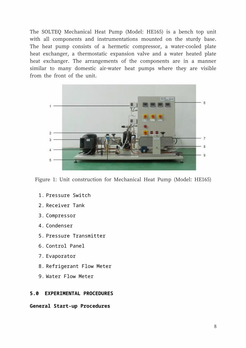
Figure 1: Unit construction for Mechanical Heat Pump (Model: HE165)

1. Pressure Switch

2. Receiver Tank

3. Compressor

4. Condenser

5. Pressure Transmitter

6. Control Panel

7. Evaporator

8. Refrigerant Flow Meter

9. Water Flow Meter

5.0 EXPERIMENTAL PROCEDURES

General Start-up Procedures

1. The unit and all instruments were checked to make sure they were in proper

condition.

2. Both water source and drain were checked to ensure that they were connected. Then

the water supply was opened and the cooling water flow rate was set at 1.0 LPM.

3. The drain hose at the condensate collector was checked to make sure it was

connected.

4. The power supply was connected and switch on the main power was switched on,

followed by main switch at the control panel.

8

5. The refrigerant compressor was switched on. The unit was considered ready for

experiment once the temperature and pressures were constant.

General Shut-down Procedures

1. The compressor, main switch and power supply were switched off.

2. The water supply was closed and it was ensured that the water was not left running.

Experiment 1: Determination of power input, heat output and coefficient of

performance

1. The general start-up procedures were performed.

2. The cooling water flow rate was adjusted to 40%.

3. The system was allowed to run for 15 minutes.

4. All necessary readings like Cooling Water Flow Rate, Cooling Water Inlet

Temperature, Cooling Water Outlet Temperature, and Compressor Power Input were

recorded.

Experiment 2: Production of heat pump performance curves over a range of source and

delivery temperatures

1. The general start-up procedures were performed.

2. The cooling water flow rate was adjusted to 80%.

3. The system was allowed to run for 15 minutes.

4. All necessary readings were recorded

5. The experiment was repeated with reducing water flow rate so that the cooling water

outlet temperature increases by about 1°C.

6. The experiment was then repeated at different ambient temperature.

Experiment 3: Production of vapour compression cycle on p-h diagram and energy

balance study

1. The general start-up procedures were performed.

2. The cooling water flow rate was adjusted to 80%.

3. The system was allowed to run for 15 minutes.

9

4. Readings like refrigerant flow rate, refrigerant pressure, refrigerant temperature,

cooling water flow rate, cooling water inlet temperature and compressor power input

were recorded.

6.0 RESULTS

Experiment 1: Determination of power input, heat output and coefficient of performance

Table 1: Data obtained and calculated for Experiment 1

Cooling Water Flow Rate, FT1 (%) 40.0

Cooling Water Flow Rate, FT1 (LPM) 2.0

Cooling Water Inlet Temperature, TT5 (oC) 28.1

Cooling Water Outlet Temperature, TT6 (oC) 29.5

Compressor Power Input, W 160.0

Heat Output, W 195.07

COPH 1.219

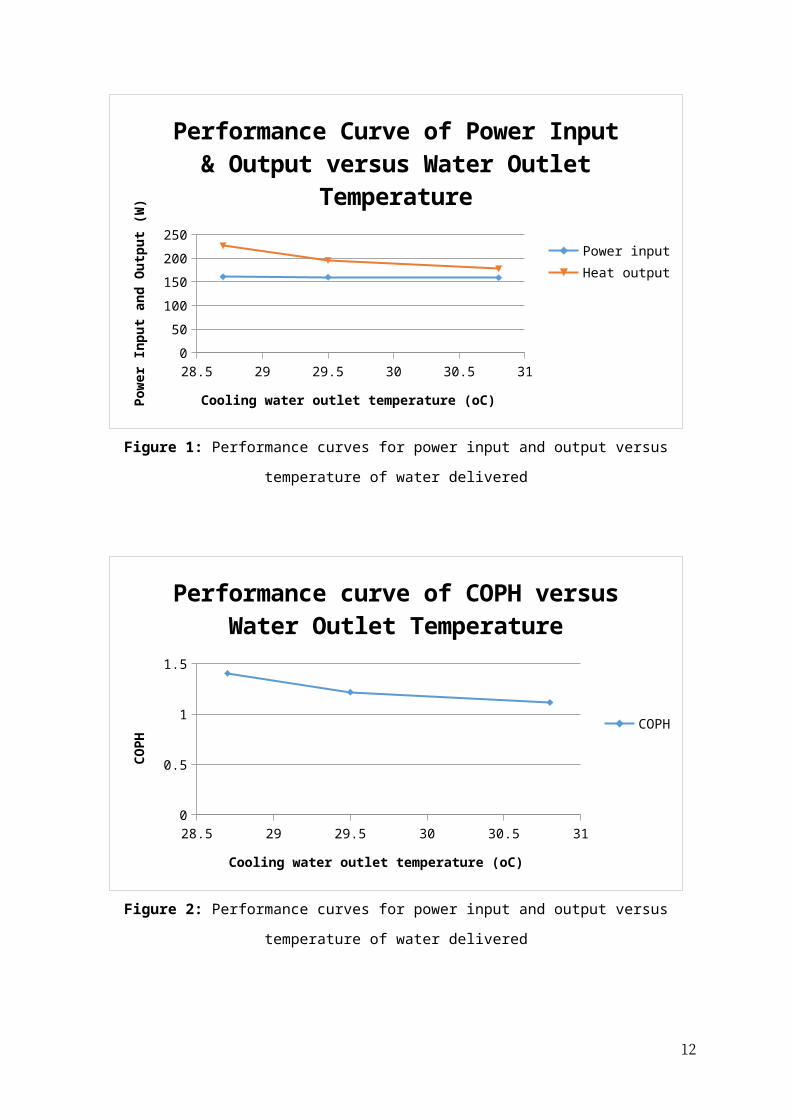
Experiment 2: Production of heat pump performance curves over a range of source and delivery

temperatures

Table 2: Data obtained and calculated for Experiment 2

Test 1 2 3

Cooling Water Flow Rate, FT1 % 30 40 50

Cooling Water Flow Rate, FT1 LPM 1.5 2 2.5

Cooling Water Inlet Temperature, TT5 oC 29.1 28.1 27.4

Cooling Water Outlet Temperature, TT6 oC 30.8 29.5 28.7

Compressor Power Input W 159.0 160.0 161.0

Heat Output W 177.65 195.07 226.42

COPH - 1.117 1.219 1.406

10

28.5 29 29.5 30 30.5 310

50

100

150

200

250

Performance Curve of Power Input & Output versus Water Outlet Temperature

Power inputHeat output

Cooling water outlet temperature (oC)

Pow

er In

put a

nd O

utpu

t (W

)

Figure 1: Performance curves for power input and output versus temperature of water delivered

28.5 29 29.5 30 30.5 310

0.2

0.4

0.6

0.8

1

1.2

1.4

1.6

Performance curve of COPH versus Water Outlet Temperature

COPH

Cooling water outlet temperature (oC)

COPH

Figure 2: Performance curves for power input and output versus temperature of water delivered

11

Experiment 3: Production of vapour compression cycle on p-h diagram and energy balance study

Table 3: Data obtained and calculated for Experiment 3

Refrigerant Flow Rate, FT2 % 60.8

Refrigerant Flow Rate, FT2 LPM 0.77

Refrigerant Pressure (Low), P1 Bar (abs) 1.8

Refrigerant Pressure (High), P2 Bar (abs) 6.8

Refrigerant Temperature, TT1 oC 25.6

Refrigerant Temperature, TT2 oC 63.1

Refrigerant Temperature, TT3 oC 28.2

Refrigerant Temperature, TT4 oC 21.5

Cooling Water Flow Rate, FT1 % 40.0

Cooling Water Flow Rate, FT1 LPM 2.0

Cooling Water Inlet Temperature, TT5 oC 28.1

Cooling Water Outlet Temperature, TT6 oC 29.5

Compressor Power Input W 160.0

50 100 150 200 250 300 3500

0.1

0.2

0.3

0.4

0.5

0.6

0.7

0.8

0.18

0.680.68

0.18 0.18

p-h diagram of R-134a

h (kJ/kg)

Pres

sure

(MPa

)

h1

h2h3

h4

Figure 3: p-h diagram of R-134a obtained from calculation

12

Table 4: Enthalpy values for each point

h1 242.86 kJ/kg

h2 301.79 kJ/kg

h3 87.40 kJ/kg

h4 87.41 kJ/kg

7.0 SAMPLE CALCULATIONS

Using sample data from Experiment 1:

Cooling water flowrate , LPM=cooling water flowrate (% )

100 %×5 LPM

¿ 40100

×5=2 LPM

Heat output=2.0 Lmin

×1kg1 L

×1 min60 sec

×4180 Jkg . K

× (29.5−28.1 ) K=195.07 W

COPH= Heat outputPower input

=195.07 W160 W

=1.219

Using sample data from Experiment 3:

Refrigerant flowrate , LPM=Refrigerant flowrate (% )

100 %×1.26 LPM

¿ 60.8100

×1.26=0.77 LPM

Ref rigerant pressure (Low )=1.8 ×̄100000 Pa

¿̄=180 kPa=0.18 MPa¿

Refrigerant pressure ( High )=6.8 ×̄100000 Pa

¿̄=680 kPa=0.68 MPa¿

Using the saturated refrigerant-134a table from Appendix 1:

h1@0.18MPa=242.86 kJ /kg

13

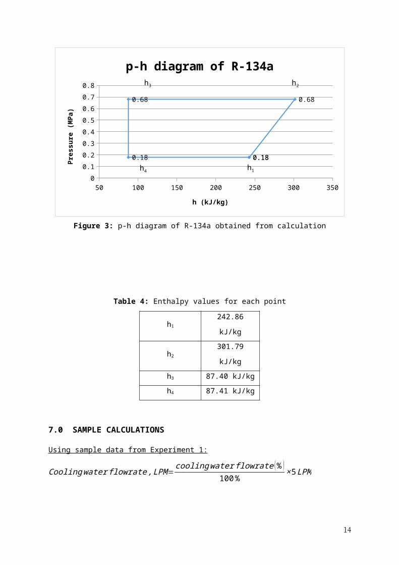
Table 5: Interpolation of data for 0.68 MPa saturated refrigerant-134a

P (MPa) h (kJ/kg)

0.65 85.26

0.68 87.40

0.70 88.82

h3@0.68 MPa=87.40 kJ /kg

Table 6: Interpolation of data for 21.5oC saturated refrigerant-134a

T (oC) hf (kJ/kg) hfg (kJ/kg) Hg (kJ/kg)

20 79.32 182.27 261.59

21.5 81.44 180.94 262.38

22 82.14 180.49 262.64

xgas=h3−hg

h f−hg

=87.40−262.3881.44−262.38

=0.967

h4 @21.5°C=hf +(1−x ) hfg=81.44+(0.033 )180.94=87.41 kJ /kg

Using the superheated refrigerant-134a table from Appendix 2:

Table 7: Interpolation of data for 0.68 MPa superheated refrigerant-134a

P (MPa) h@60oC (kJ/kg) h@70

oC (kJ/kg)

0.60 299.98 309.73

0.68 298.73 308.61

0.70 298.42 308.33

T (oC) h (kJ/kg)

60.0 298.73

63.1 301.79

70.0 308.61

14

−h60 °C @0.68 MPa=0.70−0.680.70−0.60

× (298.42−299.98 )−298.42=−298.73

h60 °C @0.68 MPa=298.73 kJ /kg

h2@63.1 °C ,0.68 MPa=301.79 kJ /kg

Energy balance on the condenser:

Refrigerant mass flow rate=3.04 Lmin

×1 min60 sec

×0.001 m3

1 L×

9.058 kgm3

¿0.4589 x10−3 kg/ s

Heat transfer ¿ refrigerant=0.4589 x10−3kgs

×1000 J

kg× (301.79−87.40 )

¿98.38 J / s

Heat transfer ¿ the cooling water= 2 Lmin

×1 Lkg

×1min60 sec

×4180 Jkg . K

× (29.5−28.1 )

¿195.07 J / s=195.07 W

Energy balance on the compressor:

Power input=160 W

Heat transfer ¿ the refrigerant=0.4589 x 10−3 kgs

×1000 J

kg× (301.79−242.86 )

¿27.04 W

Heat loss¿ surroundings=160−27.04=132.96 W

8.0 DISCUSSION

The first experiment was conducted to calculate the performance of a vapor compression heat pump

system. The power input of the heat pump obtained was 160 W while the heat output of the system

was 195.07 W. This increase in power is due to vapor compression heat pump cycle which involves 4

different processes; compression, condensation, expansion, and vaporization. At the vaporization

process, it receives heat from other sources, and the refrigerant is then subcooled at the condenser and

allows it to remove heat to the intended medium. This increase in power gives the coefficient

performance of 1.219. This would indicate that for each Watt of electrical energy supplied, 1.219 W

of heat energy is supplied to the medium to be heated. (Radermacher, 2005)

15

In the second experiment, three different flow rates in percent were used which is 30%, 40%,

and 50%. As the flow rate decrease, the cooling water outlet temperature increases whereas the power

input, heat output, and COPH decreases. The flow rate at 50%, 40%, and 30% gives the power input

reading of 161, 160, and 159 W respectively, heat output of 226.42, 195.07, and 177.65 W

respectively, and COPH of 1.406, 1.219, and 1.117 respectively. The heat output in relation to flow

rate can be expressed as:

q= hc p ρdt

Where q is the volumetric flow rate, h is heat output, cp is the specific heat capacity, ρ is density, and

dt is temperature difference. This equation shows the linear relationship between heat output and flow

rate. This in turn directly affects the COPH as the lower heat output will yield lower COPH. (“Flow

Rates in Heating System”)

The third experiment encompasses the four processes in the heat pump. The compression

process increases the pressure of refrigerant which also cause an increase in temperature. This

elevates the refrigerant into superheated state. Then, the condensation process removes the heat,

causing a decrease in temperature. The expansion valve then reduces the pressure, causing a small

portion of the refrigerant to flashes into gas. This creates a mixture of liquid and gas refrigerant. The

mixture then undergoes the vaporization process at the evaporator to receive heat energy and all

refrigerant completely vaporizes and the cycle repeats. Figure 3 shows the p-h diagram of the r-134a.

The enthalpy calculated at h1, h2, h3, and h4 are 242.86, 301.79, 87.40, and 87.41 kJ/kg respectively.

These values create a p-h diagram almost similar to the ideal cycle: (Haile, 2002)

Figure 4: Ideal vapor-compression cycle of heat pump

16

9.0 CONCLUSION

Overall, this experiment is considered success as the power input, heat output and coefficient

of performance of a vapour compression heat pump system has been determined. For the first

experiment, the power input of the heat pump obtained was 160 W while the heat output of

the system was 195.07 W. Increase in power gives the coefficient performance of 1.219. For

the second experiment, as the flow rate decrease, the cooling water outlet temperature

increases whereas the power input, heat output, and COPH decreases. The flow rate at 50%,

40%, and 30% gives the power input reading of 161, 160, and 159 W respectively, heat

output of 226.42, 195.07, and 177.65 W respectively, and COPH of 1.406, 1.219, and 1.117

respectively. The third experiment, the enthalpy calculated at h1, h2, h3, and h4 are 242.86,

301.79, 87.40, and 87.41 kJ/kg respectively. These values create a p-h diagram almost similar

to the ideal cycle.

10.0 RECOMMENDATIONS

1. Make sure that equipment is properly set up as it will affect the reading. Ask help

from the lab assistant if required.

2. Allow the system to run for 15 minutes each time before the experiment is conducted.

3. Maybe the efficiency of the equipment should be monitored frequently as some of the

readings obtained are a bit off than what we are supposed to obtain.

4. Do a trial experiment before conducting the real experiment in order to detect if there

is any error or whether the equipment is functioning well or not.

5. Make sure that the water flow rate is in stable condition as unstable water flow would

affect the readings.

11.0 REFERENCES

1. Radermacher, R., & Hwang, Y. (2005). Vapor compression heat pumps with refrigerant mixes. Boca Raton, FL: Taylor & Francis.

2. Haile, J. M. (2002). Lectures in Thermodynamics: Macatea Productions.3. Flow Rates in Heating System. (n.d.). Retrieved 27th May 2015 from

http://www.engineeringtoolbox.com/water-flow-rates-heating-systems-d_659.html

4. Thermofluids Laboratory Manual

12.0 APPENDICES

17

18