excitation optimization of a standard lrc circuit with
TRANSCRIPT
Hamline UniversityDigitalCommons@Hamline
Departmental Honors Projects College of Liberal Arts
Spring 2013
Excitation Optimization of a Standard LRC Circuitwith Impulsive Forces Selected via SimulatedAnnealingRyan M. SpiesHamline University
Follow this and additional works at: https://digitalcommons.hamline.edu/dhp
Part of the Physics Commons
This Honors Project is brought to you for free and open access by the College of Liberal Arts at DigitalCommons@Hamline. It has been accepted forinclusion in Departmental Honors Projects by an authorized administrator of DigitalCommons@Hamline. For more information, please [email protected], [email protected].
Recommended CitationSpies, Ryan M., "Excitation Optimization of a Standard LRC Circuit with Impulsive Forces Selected via Simulated Annealing" (2013).Departmental Honors Projects. 3.https://digitalcommons.hamline.edu/dhp/3

Excitation Optimization of a Standard LRCCircuit with Impulsive Forces Selected via
Simulated Annealing
Ryan M. Spies
An Honors Thesis
Submitted for partial fulfillment of the requirements forgraduation with honors in Physics from Hamline University
April 26, 2013

ii

Abstract
For an unknown oscillator, it is sometimes useful to know what thepotential energy function associated with it is. An argument forusing a method of determining the optimal sequence of impulsiveforces in order to find the potential energy function is made usingprinciples of energy. Global optimization via simulated annealingis discussed, and various parameters that can be adjusted acrossexperiments are established. A method for determining the optimalsequence of impulsive forces for the excitation of a standard LRCcircuit is established using the methodology of simulated annealing.
iii

iv

Contents
1 Motivation 11.1 Simple Harmonic Oscillator . . . . . . . . . . . . . . . . . . . . . 21.2 General Oscillator . . . . . . . . . . . . . . . . . . . . . . . . . . 41.3 LRC Extensions . . . . . . . . . . . . . . . . . . . . . . . . . . . 6
2 Methodology 92.1 Simulated Annealing . . . . . . . . . . . . . . . . . . . . . . . . . 9
2.1.1 Acceptance Probability . . . . . . . . . . . . . . . . . . . 102.1.2 Annealing Schedule . . . . . . . . . . . . . . . . . . . . . 112.1.3 Neighborhood Selection . . . . . . . . . . . . . . . . . . . 11
2.2 Electronics . . . . . . . . . . . . . . . . . . . . . . . . . . . . . . 122.2.1 Circuitry . . . . . . . . . . . . . . . . . . . . . . . . . . . 122.2.2 Arduino Program . . . . . . . . . . . . . . . . . . . . . . . 14
2.3 Main Python Program . . . . . . . . . . . . . . . . . . . . . . . . 15
3 Results 173.1 How to Interpret Simulation Results . . . . . . . . . . . . . . . . 173.2 Results of Simulation . . . . . . . . . . . . . . . . . . . . . . . . . 19
3.2.1 1st Simulation Run . . . . . . . . . . . . . . . . . . . . . . 193.2.2 2nd Simulation Run . . . . . . . . . . . . . . . . . . . . . 203.2.3 3rd Simulation Run . . . . . . . . . . . . . . . . . . . . . 213.2.4 4th Simulation Run . . . . . . . . . . . . . . . . . . . . . 223.2.5 5th Simulation Run . . . . . . . . . . . . . . . . . . . . . 233.2.6 6th Simulation Run . . . . . . . . . . . . . . . . . . . . . 243.2.7 7th Simulation Run . . . . . . . . . . . . . . . . . . . . . 253.2.8 8th Simulation Run . . . . . . . . . . . . . . . . . . . . . 263.2.9 9th Simulation Run . . . . . . . . . . . . . . . . . . . . . 273.2.10 10th Simulation Run . . . . . . . . . . . . . . . . . . . . . 283.2.11 11th Simulation Run . . . . . . . . . . . . . . . . . . . . . 293.2.12 12th Simulation Run . . . . . . . . . . . . . . . . . . . . . 303.2.13 13th Simulation Run . . . . . . . . . . . . . . . . . . . . . 313.2.14 14th Simulation Run . . . . . . . . . . . . . . . . . . . . . 323.2.15 15th Simulation Run . . . . . . . . . . . . . . . . . . . . . 333.2.16 16th Simulation Run . . . . . . . . . . . . . . . . . . . . . 343.2.17 17th Simulation Run . . . . . . . . . . . . . . . . . . . . . 353.2.18 18th Simulation Run . . . . . . . . . . . . . . . . . . . . . 363.2.19 19th Simulation Run . . . . . . . . . . . . . . . . . . . . . 373.2.20 20th Simulation Run . . . . . . . . . . . . . . . . . . . . . 38
v

vi CONTENTS
3.2.21 21st Simulation Run . . . . . . . . . . . . . . . . . . . . . 393.2.22 22nd Simulation Run . . . . . . . . . . . . . . . . . . . . . 403.2.23 23rd Simulation Run . . . . . . . . . . . . . . . . . . . . . 413.2.24 24th Simulation Run . . . . . . . . . . . . . . . . . . . . . 423.2.25 25th Simulation Run . . . . . . . . . . . . . . . . . . . . . 433.2.26 26th Simulation Run . . . . . . . . . . . . . . . . . . . . . 443.2.27 27th Simulation Run . . . . . . . . . . . . . . . . . . . . . 453.2.28 28th Simulation Run . . . . . . . . . . . . . . . . . . . . . 463.2.29 29th Simulation Run . . . . . . . . . . . . . . . . . . . . . 473.2.30 30th Simulation Run . . . . . . . . . . . . . . . . . . . . . 483.2.31 31st Simulation Run . . . . . . . . . . . . . . . . . . . . . 493.2.32 32nd Simulation Run . . . . . . . . . . . . . . . . . . . . . 50
3.3 General Remarks on Simulation Results . . . . . . . . . . . . . . 513.4 Results of Physical Experiment . . . . . . . . . . . . . . . . . . . 513.5 Analysis of Physical Experiment . . . . . . . . . . . . . . . . . . 54
4 Discussion 574.1 Conclusions . . . . . . . . . . . . . . . . . . . . . . . . . . . . . . 574.2 Next Steps With this Methodology . . . . . . . . . . . . . . . . . 584.3 Future Directions . . . . . . . . . . . . . . . . . . . . . . . . . . . 58
A Simulated Annealing Test Algorithm 59
B Main Experiment Python Code 67
C Arduino Module Code 73
D Arduino Sketch Code 75
E Mathematica Analysis for Experiment 77

List of Figures
2.1 Pseudo-Python implementation of the standard simulated an-nealing algorithm for finding a global minimum. . . . . . . . . . . 10
2.2 Circuit diagram of the follower circuit attached to the RLC circuit. 13
3.1 The graph of the interpolated function that was explored in thealgorithm in Appendix A. The x-axis is the solution space, andthe y-axis is the corresponding fitness for any given part of thesolution space. Note the global maximum at approximately 8. . . 18
3.2 Results of 1st Experiment . . . . . . . . . . . . . . . . . . . . . . 193.3 Results of 2nd Experiment . . . . . . . . . . . . . . . . . . . . . . 203.4 Results of 3rd Experiment . . . . . . . . . . . . . . . . . . . . . . 213.5 Results of 4th Experiment . . . . . . . . . . . . . . . . . . . . . . 223.6 Results of 5th Experiment . . . . . . . . . . . . . . . . . . . . . . 233.7 Results of 6th Experiment . . . . . . . . . . . . . . . . . . . . . . 243.8 Results of 7th Experiment . . . . . . . . . . . . . . . . . . . . . . 253.9 Results of 8th Experiment . . . . . . . . . . . . . . . . . . . . . . 263.10 Results of 9th Experiment . . . . . . . . . . . . . . . . . . . . . . 273.11 Results of 10th Experiment . . . . . . . . . . . . . . . . . . . . . 283.12 Results of 11th Experiment . . . . . . . . . . . . . . . . . . . . . 293.13 Results of 12th Experiment . . . . . . . . . . . . . . . . . . . . . 303.14 Results of 13th Experiment . . . . . . . . . . . . . . . . . . . . . 313.15 Results of 14th Experiment . . . . . . . . . . . . . . . . . . . . . 323.16 Results of 15th Experiment . . . . . . . . . . . . . . . . . . . . . 333.17 Results of 16th Experiment . . . . . . . . . . . . . . . . . . . . . 343.18 Results of 17th Experiment . . . . . . . . . . . . . . . . . . . . . 353.19 Results of 18th Experiment . . . . . . . . . . . . . . . . . . . . . 363.20 Results of 19th Experiment . . . . . . . . . . . . . . . . . . . . . 373.21 Results of 20th Experiment . . . . . . . . . . . . . . . . . . . . . 383.22 Results of 21st Experiment . . . . . . . . . . . . . . . . . . . . . 393.23 Results of 22nd Experiment . . . . . . . . . . . . . . . . . . . . . 403.24 Results of 23rd Experiment . . . . . . . . . . . . . . . . . . . . . 413.25 Results of 24th Experiment . . . . . . . . . . . . . . . . . . . . . 423.26 Results of 25th Experiment . . . . . . . . . . . . . . . . . . . . . 433.27 Results of 26th Experiment . . . . . . . . . . . . . . . . . . . . . 443.28 Results of 27th Experiment . . . . . . . . . . . . . . . . . . . . . 453.29 Results of 28th Experiment . . . . . . . . . . . . . . . . . . . . . 463.30 Results of 29th Experiment . . . . . . . . . . . . . . . . . . . . . 473.31 Results of 30th Experiment . . . . . . . . . . . . . . . . . . . . . 48
vii

viii LIST OF FIGURES
3.32 Results of 31st Experiment . . . . . . . . . . . . . . . . . . . . . 493.33 Results of 32nd Experiment . . . . . . . . . . . . . . . . . . . . . 503.34 1st pulse timing selection . . . . . . . . . . . . . . . . . . . . . . 523.35 2nd pulse timing selection . . . . . . . . . . . . . . . . . . . . . . 523.36 3rd pulse timing selection . . . . . . . . . . . . . . . . . . . . . . 533.37 4th pulse timing selection . . . . . . . . . . . . . . . . . . . . . . 533.38 5th pulse timing selection . . . . . . . . . . . . . . . . . . . . . . 543.39 Electric potential fit . . . . . . . . . . . . . . . . . . . . . . . . . 55
4.1 Plot of voltage for this LRC . . . . . . . . . . . . . . . . . . . . . 57

Chapter 1
Motivation
We want to develop a methodology that will allow us to determine the optimalsequence of pulse timings for an oscillator, which will in turn determine theoptimal motion for the oscillator as well. This methodology must also allow usto find the potential energy function of a given oscillator. In order to understandwhat it means to determine the optimal sequence of pulse timings, we must firstunderstand the dynamics of oscillators. In particular, we want to understandthe dynamics of oscillators after they are hit by an impulsive force. Also, wewant to know what it means to find the potential energy function for a givenoscillator, and to figure out how that is related to the problem of finding theoptimal sequence of pulse timings. Finally, we want to understand what itmeans to take the principles of these classical oscillator problems and applythem to electronic oscillators.
For a thought experiment, let us consider a pendulum. If we gave thispendulum a slight push, and if there is no friction present, then the pendulumwill move and the motion will not decrease. If we want to get this pendulumto swing out further we want to push it more, but then comes the matter ofdetermining when it is best to push the pendulum again. Assuming that thependulum can only be pushed from one direction, the best moment for pushingit again would be when it is back at its equilibrium position and when it isgoing in the same direction as the push. However, since the pendulum hasa periodic behavior that is nonlinear for sufficiently large angles (so that theapproximation for the angular position θ of the pendulum, θ ≈ sin(θ), or theangles for which simple harmonic motion occurs, no longer holds) the timingof these pushes becomes a problem. The amount of time that one would haveto wait before pushing the pendulum again at the best time changes, so thismotivates a method that can find when to push the pendulum without priorknowledge of the pendulum’s behavior.
In order to understand how our thought experiment relates to the largerproblem let us consider the dynamics of oscillators in general, and start withthe example of the simple harmonic oscillator.
1

2 CHAPTER 1. MOTIVATION
1.1 Simple Harmonic Oscillator
The motion of the simple harmonic oscillator can be determined by first findingthe sum of forces that are acting on the oscillator. For the simple harmonicoscillator there is only one force acting on it. This is the force due to the springattached to the mass. Our sum of forces equation can now be written as:
ΣF = −kx = mx, (1.1)
In equation 1.1 F is the force, k is Hooke’s constant for that spring, m is themass of the oscillator, and x is the one-dimensional position of the oscillator.The dots represent the second derivative with respect to time t. We can useequation 1.1 to find the equation of motion:
mx = −kx. (1.2)
This is then rewritten to obtain:
mx+ kx = 0. (1.3)
Equation 1.3 is a homogenous ordinary second-order differential equationthat can be solved to find x. In classical mechanics we can also refer to thisequation as the unforced case for the simple harmonic oscillator. Using methodsfor solving ordinary differential equations the position x as a function of timecan be determined in terms of the various constants that govern the differentialbehavior of the oscillator.
However, this is not the case of the oscillator that we want to investigatein this experiment. Instead, we want to investigate a particular instance of theforced oscillator where the oscillator is driven by a sequence of impulsive forces.The differential equation for this case is:
mx+ kx = Fτ(t). (1.4)
Here F is a constant in units of force that represents the magnitude of theimpulsive force, the timing function, τ(t), is a unitless function that is writtenas a series of Dirac delta functions:
τ(t) = δ(t0) + δ(t1) + δ(t2) + ... (1.5)
In equation 1.5 the moments in time ti (where i = 0, 1, 2, ...) are when animpulsive force occurs. It is important to note that this particular function isa model for showing when impulsive forces happen. For any physical examplesan impulsive force is simply a force that delivers a lot of momentum over ashort length of time in comparison to the overall duration of the motion that isconsidered.
The ultimate goal of the experiment is to find the series of optimal ti forexciting an oscillator. In order to determine at which moments an impulsiveforce needs to act on an object for obtaining the optimal response, we must firstconsider the effect that an impulsive force has on the overall momentum of anobject. If we integrate the impulsive force over time we get that the impulsethat is added to the oscillator is:∫
F dt = F∆t.

1.1. SIMPLE HARMONIC OSCILLATOR 3
Here ∆t is the length of a brief interval in time during which the impulsive forceacts.
When the impulsive force F is delivered the final momentum pf of the os-cillator will then be:
pf = pi + F∆t, (1.6)
where pi is the initial momentum at the moment of the impulse. Both sides canbe rewritten in terms of energy. We can then consider the final energy Ef ofthe oscillator after the impulsive force gives the system an amount of energy uito be:
Ef =p2i2m
+ ui. (1.7)
In order to optimize the motion of the oscillator, the energy ui that is de-livered to the oscillator must be maximized. In order to determine how tomaximize this energy we first take a look at the change in energy that occursdue to the impulsive force:
∆E =p2f − p2i
2m=p2i + 2F∆tpi + F 2∆t2 − p2i
2m,
which we rewrite as:
∆E =2F∆tpi + F 2∆t2
2m. (1.8)
For our one-dimensional case we can leave equation 1.8 as is and recognizethat when the initial momentum pi is at its maximum then the change in energyis maximized as well. For two or three dimensional problems we can use vectoralgebra to rewrite 1.8 as:
∆E =2∆t ~F · ~pi + F 2∆t2
2m. (1.9)
In equation 1.9 it is apparent that in order to maximize the change in energy,the dot product of the impulsive force and the initial momentum at the momentof the impulsive force must also be maximized. This means that in order toexcite an oscillator with impulsive forces, those forces must also be applied insuch a way that they will be in the same direction as the initial momentum atthe time of the impulsive force. This generalization to two or three dimensionsapplies to our one dimensional problem as well.
Given the conditions that must be met in order to maximize the momen-tum after the delivery of an impulsive force, we can determine the sequence ofimpulsive forces that will optimize the motion of our oscillator. We first solveequation 1.3 for x. In order to do this we will first define a new quantity ω0, orthe resonant frequency of the oscillator:
ω0 =
√k
m.
We can use this substitution to rewrite equation 1.3 as:
x+ ω20x = 0. (1.10)
The general solution to this is:
x(t) = A sin(ω0t+ φ). (1.11)

4 CHAPTER 1. MOTIVATION
In equation 1.11 A is some maximum amplitude, and φ is some change inphase. These constants can be determined using initial conditions. From thispoint on we will consider an amplitude of one and a phase change of zero. Wemust now consider finding when the velocity is maximized, which can be deter-mined by finding the acceleration. We take the first and second derivatives tofind the velocity and acceleration of the simple harmonic oscillator respectively.
x = ω0 cos(ω0t) (1.12)
x = −ω20 sin(ω0t) (1.13)
We find the first point at which equation 1.13 is zero and equation 1.12 ispositive in order to find the point in time at which the velocity, and thereforethe momentum is maximized. Our system will look like the following:
0 < ω0 cos(ω0t) (1.14)
0 = −ω20 sin(ω0t) (1.15)
The system of equations is solved to obtain that the first moment in timewhere both of these conditions are met is the time when the oscillator completesthe first full period. We refer to this time as tp, which we can write out as:
tp =2π
ω0.
By the conclusions that we arrived at earlier with equations 1.8 and 1.9, theoptimal timing function is:
τ(t) = δ(tp) + δ(2tp) + δ(3tp) + ... (1.16)
1.2 General Oscillator
Now that we have established the basic premise for maximizing the responseof the linear oscillator, let us consider a more general case where instead ofbehaving like a linear spring there is a non-linear response. Before we can dothis, we must first consider the simple harmonic oscillator in terms of a potentialenergy function so we can understand the general oscillator problem. In generalwe can write the potential energy function U of a conservative force as:
U(x) = −∫
~F (x) · d~x. (1.17)
For our simple harmonic oscillator we can find the potential energy functionof the spring using equation 1.17.
U(x) = −∫−kx dx
U(x) =1
2kx2. (1.18)
We also get from equation 1.17 that the relationship between a conservativeforce and a potential energy can be written as:
~F = −~∇U, (1.19)
1.2. GENERAL OSCILLATOR 5
or in one dimension:
F = −dUdx
. (1.20)
For an oscillator whose motion is determined by a conservative force, assum-ing no friction, we get that the equation of motion is:
mx+dU
dx= 0. (1.21)
Sometimes for the case of the general oscillator, and in particular when non-linear behavior is present in the motion of the oscillator, we do not always knowthe potential energy function. However, there is a relationship between theamplitude of an oscillator and the kinetic energy that is given to an oscillatorthat can be exploited in order to determine the potential energy function of theoscillator. If we give an oscillator a discrete amount of energy each time andthen we record the maximum amplitude attained by the oscillator then we canuse these data points to fit a curve for the potential energy.
In order to show that we can do this, we first look at the general equationfor the total energy in a system. We define the kinetic energy K as:
K =p2
2m
Our total energy is then:
E =p2
2m+ U. (1.22)
The total energy in any system can be expressed as a sum of the kineticand potential energy at any moment in time. Now we examine the energy at aparticular point in time. If there is a discrete amount of energy that is presentin a system, and if we can assume that none of that energy is lost to friction,then we can conclude that there are moments in time where all the energy iskinetic energy and where all the energy is potential energy. For the momentswhere all the energy is kinetic we know that:
E =p2max
2m. (1.23)
We can conclude this because at this moment the momentum of the systemis maximized since all of the energy present in the system is kinetic. We alsoknow from the work in the previous section that at the moment the momentumis maximized, that it would be the best time to deliver an impulsive force tofurther increase the motion of the oscillator. This establishes that we require amethod that determines the optimal timing in order to maximize the change inenergy, and to make sure that the change in energy with each impulsive force isthe same.
In order to determine the potential energy function from an experimentwhere the optimal sequence of impulsive forces is determined, we must alsoexamine what happens at moments when the total energy is all potential energy.In an oscillator that assumes that the effects of friction on the total energy isnegligible, when we have established that after an impulsive force the kineticenergy that can be present after that force is at a maximum, we know then
6 CHAPTER 1. MOTIVATION
that the potential energy at a later point will also be at a maximum. Statedmathematically this is:
E = U. (1.24)
At these moments the oscillator is at it’s maximum position, which allowsus to rewrite equation 1.24 in terms of position as:
E = U(xmax). (1.25)
This means that in order to find the potential energy as a function of position,an experiment must also include a way to measure the position after an impulsiveforce is delivered. After gathering the maximum positions after each impulsiveforce the total energy as a function of position can be determined via numericalmethods such as interpolation, and this function is equivalent to the potentialenergy function as a function of position.
1.3 LRC Extensions
This experiment will utilize a LRC circuit as the oscillator. In order to under-stand the behavior of this circuit, it is first important to note that there is africtional element present in the system that removes energy. In order to under-stand the impact that a frictional element will have on the overall motion of thesystem, it is important to consider the full equation for the damped harmonicoscillator:
mx+ bx+ kx = 0. (1.26)
In this equation the value b corresponds to a drag constant, which determines byhow much the corresponding drag force removes energy from the system. Thedrag force for this classical case is the friction due to the surrounding medium.
We now consider the equation for the voltage behavior of a charged LRCcircuit:
Lq +Rq +1
Cq = 0. (1.27)
Here L is the inductance, R is the resistance, C is the capacitance, and q is thecharge. From here we can begin to make a few analogies that tie the LRC to theclassical damped harmonic oscillator problem, and how to determine energiesand potential energy functions.
To begin with L corresponds to m, which also gives us the following analogyfor kinetic energy K in an electronic system;
K =1
2LI2.
Here I is the current, or the first time derivative of charge. The charge q, andits derivatives take on the role of the position x in the electronic system.
In the classical damped oscillator problem, we can determine the work Wthat is removed from the system by evaluating the following integral:
W =
∫bx dx.

1.3. LRC EXTENSIONS 7
It is important to note that we can rewrite the differential element dx in termsof time. This can simply be achieved by taking the first derivative of x and thenmultiplying it by dt. This gives us the new integral:
W =
∫bx2 dt. (1.28)
Therefore, if we can obtain x as a function of time, a derivative of that canbe taken and this integral can be solved to keep track of how much work waseliminated due to friction as time goes on. By our analogy with the LRC, Rtakes on the role of b. This means that for our electronic analog we get for thework removed from the system over time:
W =
∫RI2 dt. (1.29)
Finally, we have the matter of determining the potential energy function.We continue our analogy to note that k is related to the inverse of C. Thepotential energy function for our system is then:
U =q2
2C. (1.30)
This is related to the electrical potential V by dividing by q.Now we must determine how to find the electrical potential from our pro-
posed experiment as a function of the charge q. We must first be able to deter-mine the charge at any point during the experiment. For this, we consider thecharging behavior of the LRC circuit, and from there we can determine whatthe charge present is at any point. We now consider a particular case of theLRC where:
Lq +Rq +1
Cq = V0τ(t). (1.31)
Here V0 is a constant value for the potential. This driven case of the LRC circuitis the electronic form of our driven harmonic oscillator problem, only with somefrictional element included. When the circuit is driven by a voltage impulse,it is considered to be a pure DC circuit. This means that the effects of theinductor can be ignored while it is in this state. We obtain that the voltage asa function of time for while the voltage impulse is present is then:
V (t) = V0(1− e−t/RC). (1.32)
Since the charge present in a capacitor is found by:
q = V C,
It follows that:q(t) = CV0(1− e−t/RC), (1.33)
when the capacitor is charging. As the capacitor discharges over time from thetotal amount of charge q0 we can state that the total charge present is then:
q(t) = q0e−tR/2L cos(
t√LC
), (1.34)

8 CHAPTER 1. MOTIVATION
which is the to equation 1.31 for the appropriate boundary conditions.When we have an impulsive voltage, we can determine what the charge will
be after a given point in time. Let us suppose that before an impulsive chargeis given, that the total charge present is some discrete amount qi. We then getthat for after an impulsive charge is delivered:
qf = qi + CV0(1− e−ti/RC), (1.35)
where qf is the final amount of charge present and ti is the duration of theimpulse. If measurements are taken after that, then the charge present at thetime of a particular measurement will be:
q(t) = qfe−tR/2L cos(
t√LC
). (1.36)
For an experiment where the voltage is measured, and the time at which themeasurement was taken can be obtained, then the charge at this point can alsobe found. This allows to find the electric potential as a function of charge, andby extension will allow us to find the potential energy function as a function ofcharge as well.

Chapter 2
Methodology
For our experiment, the oscillator of choice is an RLC circuit driven by a se-quence of impulsive charges that are controlled by the Arduino microcontroller.Our optimization algorithm, implemented in Python version 2.6, is a simulatedannealing algorithm that allows the user to control various stages of the al-gorithm across experiments. Both versions for simulations and for the actualexperiment are developed, with the code of each version located in the appen-dices.
2.1 Simulated Annealing
The method used for selecting the sequence of pulses used to excite the oscil-lator is simulated annealing. Simulated annealing is an optimization methodthat mimics the thermodynamic process of annealing with the goal of finding aparticular global optimum within a solution space. This solution space variesfrom implementation to implementation. A general process for simulated an-nealing for finding a global minimum is outlined in the pseudocode example inFigure 2.1. Upon initialization, the algorithm makes a guess x from the prob-lem’s solution space and computes the value of the fitness function f(x) (alsoreferred to as the cost function) for that particular guess. In addition to that atemperature T that represents how much energy is available at the start of thealgorithm is determined.
After the initial guess a loop is begun that starts by generating a neighbor-hood, or a subset of the solution space that is centered about the current ac-cepted guess. A new guess is selected from this neighborhood, and subsequentlythe fitness of this new guess is computed as well. The difference between thetwo fitnesses ∆f is then calculated as per the calculation of the quantity changein figure 2.1. For the algorithm in the pseudocode example, if this change isnegative the new guess is always accepted. If the change is non-negative, inorder to encourage exploration of the solution space within the algorithm thechance of accepting this ”worse” guess is found using a Boltzmann-like proba-bility distribution as described in the following equation:
P (∆f) = exp
(−∆f
kT
)(2.1)
9

10 CHAPTER 2. METHODOLOGY
procedure s imulated annea l ing (T, s o l u t i o n space )select guess from s o l u t i o n spacef i t n e s s = f ( guess )loop un t i l T < te rminat ion cond i t i on :
generate neighborhood about guessselect newGuess from neighborhoodnewFitness = f ( newGuess )change = newFitness−f i t n e s si f change < 0 :
accept newGuesse l i f exp(−change/kT) > random (0 , 1 ) :
accept newGuessdecrease T
return best guess and best f i t n e s s
Figure 2.1: Pseudo-Python implementation of the standard simulated anneal-ing algorithm for finding a global minimum.
In equation 2.1 k is the Boltzmann constant. In general, the algorithm canhave other solution selection methods other than the one defined in our exam-ple. After determining whether or not the guess is accepted, the temperatureis decreased and the loop repeats until the temperature is cooler than the ter-mination condition. By the end of the algorithm the best guess that it made isreturned along with the corresponding fitness. This algorithm can also be ad-justed for finding the global maximum of a particular solution space by alwaysaccepting the new guess if the change is positive, and by changing the negativesign in equation 2.1 to a positive sign.
There are a wide variety of things that can be altered about this simplealgorithm. These include determining the chance of keeping a guess, how todecrease the temperature, how to select the neighbourhood for a particularguess, and initializing the relevant constants for these. An example of a flexiblealgorithm in Python that allows a user to make the changes mentioned in thefollowing sections can be seen in Appendix A.
2.1.1 Acceptance Probability
For the typical simulated annealing algorithm, a probability selection methodthat comes from another algorithm called the Metropolis algorithm is used. Forthe problem of finding the global maximum of a particular solution space theprobability P of selection is defined as:
P (x, y, T ) =
1, y > x
exp(y−xkT
), y < x.
(2.2)
In equation 2.2, x is the previous guess and y is the most recent guess. This isa mathematical representation of the guess selection process outlined in figure2.1, and this the most frequently used guess selection probability method insimulated annealing. In addition to that method, a slightly modified probabilitydistribution method was used whose Python implementation can be found online 47 of Appendix A. Mathematically, this method can be written as:

2.1. SIMULATED ANNEALING 11
P (x, y, T ) =
1− exp
(x−ykT
), y > x
exp(y−xkT
), y < x.
(2.3)
For the method defined by equation 2.3 the probability of keeping a guessbetter than the previous one is not one, but instead one minus the probabilityof choosing a worse guess that has the same absolute value of the difference infitness from the previous guess. This allows for some variety in the experimentsthat can be performed.
2.1.2 Annealing Schedule
The annealing schedule (also known as the cooling schedule) is the way bywhich the algorithm decreases the temperature for each run of the loop. Thetwo methods most commonly used are the exponential annealing schedule andthe linear annealing schedule.
The exponential annealing schedule causes the temperature to decay ex-ponentially over the course of the algorithm. A constant c between 0 and 1(typically 0.95 for most implementations) is chosen, and at the end of each runof the loop the current temperature is multiplied by this constant. This methodof decreasing can be written as:
Tnew = cTprevious. (2.4)
The linear annealing schedule causes the temperature to decrease linearlyover the course of the algorithm. An amount ∆T is subtracted from the temper-ature as the algorithm progresses, and this rule for determining the temperaturecan be mathematically written as:
Tnew = Tprevious −∆T. (2.5)
The algorithm in Appendix A allows for a choice between the exponential andlinear schedules as defined by the function on line 160, but the main experimentutilizes an exponential schedule with a constant c of 0.95.
2.1.3 Neighborhood Selection
The last thing that is varied in the simulated annealing algorithm is the neigh-borhood selection method. This is the method by which the algorithm finds newsolutions to test. In a typical simulated annealing algorithm the neighborhood isalways a constant interval centered about the current accepted guess. However,if the neighborhood is adjusted over the course of the algorithm to decrease insize as the temperature decreases, then the algorithm performs better than ifthe algorithm has a fixed neighborhood size. This was established in the paper”Dynamic Neighbourhood Size in Simulated Annealing” by Xin Yao.
There are several different methods for neighborhood selection that are uti-lized in the algorithm that is written up in Appendix A. The first of these issimply using a constant interval that is recreated every time that the algorithmrestarts. The programmer selects some number that represents the distanceaway from the current guess in the solution space in both directions (for a one

12 CHAPTER 2. METHODOLOGY
dimensional space), and then the algorithm selects a different solution to testfrom this neighborhood.
The other approaches all rely on functions that decrease in size as T de-creases. Each of these approaches uses another user-defined constant, m, whichfor this set of experiments has the experiment start by exploring a neighbor-hood that is one quarter of the size of the solution space. One of these optionsis recreating the interval bounds at each time as a function of T proportionalto the square root of T as follows:
N =
√T
m, (2.6)
where N is the size of the neighborhood.There are a few other functions that have similar limit behavior to the square
root function as T decreases. The reason for these functions is to test an algo-rithm where the neighborhood decreases as T decreases, or in terms of limits:
limT→0
N(T ) = 0. (2.7)
This motivates us to explore a few other functions that have this behavior.In the algorithm in Appendix A three additional functions for determining thelimits of the neighborhood that have this limit behavior as defined in equation2.7. First, one of these has a linear proportionality with respect to T , or simplythat:
N = mT. (2.8)
Secondly, another method is proportional to T 2, or as defined within the algo-rithm:
N =T 2
m. (2.9)
The last of these methods uses a decreasing exponential function. This functionas defined within the algorithm is:
N = me−1T (2.10)
The last method for neighborhood selection was one where the neighborhoodwas selected so that it was increasing each time. This was meant both tosee what the algorithm behavior would be if the neighborhood increased as afunction of T and to test what would happen if at the end the entire solutionspace was available for the algorithm to choose from. In the physical experiment,this method was not selected. The function that is defined for this is:
N =m
T√
2πe−
12T2 . (2.11)
The user is capable of selecting any of these neighborhood selection methodsat the beginning of the algorithm.
2.2 Electronics
2.2.1 Circuitry
The circuit tested was a simple LRC circuit, but in order to be able to ma-nipulate and interact with this circuit via computer control the Arduino Uno

2.2. ELECTRONICS 13
microcontroller had to be used. This placed some limitations on the sort ofcircuit that can be constructed.
First, the frequency of the LRC was limited because the Arduino can onlysample once every 100µs. In order to gain a sufficient range of data from whichan optimal value can be obtained, the parts were selected as follows:
R = 10Ω, L = 3.9mH, C = 6.5µF.
In addition, there were limits to the sorts of voltages that could be obtainedby the Arduino. The Arduino uses an on board analog to digital converter thatcan only sample from 0V up to 5V. Therefore, negative voltages make it so thatwe must design a circuit that will always give a positive voltage. In order to takeadvantage of the full capability of the Arduino, this meant that the LRC hadto be set at a reference of 2.5V. This means that instead of the LRC going toground, it instead goes to a voltage supply that will remain at a constant 2.5V.In order to drive the circuit with pulses, another voltage supply was needed thatcould switch between providing 5V and 2.5V, and that this switching behaviorcould also be controlled via the Arduino.
In order to provide voltage supplies that could provide the necessary voltagebehavior and the currents that were needed for this particular circuit, a coupleof operational amplifiers (LF741) were used to make two follower circuits. Theresulting circuit using these follower circuits is diagrammed in Figure 2.2.
+5V
10kΩ 10kΩ
Arduino Output
−
+
10Ω
3.9mH
6.5µF
−
+
10kΩ
+5V
10kΩ
Figure 2.2: Circuit diagram of the follower circuit attached to the RLC circuit.
A follower circuit is one that keeps track of the voltage on one terminal, andthen outputs that exact same voltage. On the positive input is a voltage divider
14 CHAPTER 2. METHODOLOGY
that is selected so that the voltage at that terminal is 2.5V. For the followercircuit that was used for providing a constant reference voltage this consistedof two 10kΩ resistors, one coming from a constant supply of 5V and anotherattached to ground. The positive input is connected to the place on the voltagedivider where the voltage is 2.5V. For the follower circuit that provided thepulses to drive the circuit, the other end of the voltage divider was attachedto a digital output from the Arduino. This output would be at logic 0, or atground, for most of the time, and would be at logic 1, which is 5V for thisArduino, when a pulse is given. Once the positive inputs are established, aconnection between the negative input and the output of the op-amp is used.The results are two circuits that behave like the voltage sources that are neededfor this particular problem.
The two ends of the LRC were then attached to the outputs of the followercircuits. The Arduino could then be used to monitor the voltage along any pointof the circuit.
2.2.2 Arduino Program
The final part of the circuitry was to set up the Arduino properly with the correctprogram. As a microcontroller, the digital electronics within are controlled byprograms (called sketches) that are written by the user using C++ and somespecial libraries therein that are specific to Arduino programming. The fullArduino sketch can be seen in Appendix D.
The program begins with the setup section, which determines some behaviorsof the microcontroller that will only be executed at the beginning of the sketch.In this instance, the serial port is set to as high a speed as a computer canhandle, and a pin is selected to be an output for driving the LRC. After thata function called pulse() is established, which takes an output pin and turns iton for a length of time before shutting off again.
The second part of the program is one that will repeat in a loop, meaningthat this can be used to run multiple experiments. First, the microcontrollerwaits for something to be available on the serial port. From the python programthis string will be something that looks as so:
3[100, 200, 300]20.
The first number in the incoming string is interpreted to be the number oftimings between pulses, and in this case there are three timings. Then thenumbers contained within the brackets are the timings between particular pulsesin microseconds, which in this case is 100, 200, and 300 respectively. The lastnumber is interpreted as how many points of data should be obtained for thisparticular run.
After the numbers are interpreted the program then initiates a loop structurein which a pulse of five microseconds occurs, and then it cycles through anarray of timings to figure out how long to wait before the next iteration of theloop. Once this loop is complete one final pulse is given. Then the programimmediately gathers data that is sent back to the computer for interpretation.

2.3. MAIN PYTHON PROGRAM 15
2.3 Main Python Program
In appendices B and C are two parts of a program that is used to interact withthe Arduino on the computer side. Appendix B is the main simulated annealingprogram, and Appendix C is a module that defines a function that allows theprogram to interact with the Arduino.
The program starts off by defining a lot of the same functions that weredefined in the algorithm in Appendix A. After that is where the programs startto differ. Instead of allowing the user to reset the temperature at will, the tem-perature for each run of the simulated annealing algorithm will always start at10. The user is also unable to adjust the constant k for selection probabilityand the constant m for each neighborhood selection method. The terminationcondition is also fixed for this particular program. The user is allowed to varyamong various neighborhood selection methods, acceptance probability calcula-tion methods, file names, and data points gathered for the fitness function.
In this program, simulated annealing is used in nested loop structures tobuild a pulse train, or a sequence of pulses with particular timings associatedwith each of them. The user specifies under the ”how many pulses are in thepulse train” portion of the program how many timings in between pulses willbe specified.
The first loop structure will define how many times the experiment is re-peated. If the user only wants to run the experiment once, they will only runthe experiment once. Otherwise, they can specify a nonzero integer amount oftimes to repeat the experiment for.
The second loop structure within the first loop is the one that finds thesolution for a particular number of pulse timings j. It begins by making an initialguess for the jth element as defined by the loop iterator, and then determiningthe fitness. The graph and spreadsheet for this particular element of the solutionis also created within this loop structure.
The final loop structure that is within the second loop is the actual simulatedannealing algorithm itself. The simulated annealing process is repeated for eachelement of the pulse train. This allows for the solution to be built up elementby element instead of all at once.

16 CHAPTER 2. METHODOLOGY

Chapter 3
Results
3.1 How to Interpret Simulation Results
These results of this simulation are from 32 different runs of the algorithm pre-sented in Appendix A. Figure 3.1 is the graph of the fitness function that thisalgorithm explored. The temperature is the given value of T at the start of therun, and the Boltzmann Constant was the given value of k for that experiment.The interval weight was a value of m that was selected for the various meth-ods of neighborhood selection that were discussed in the methodology section.This algorithm allowed for the selection of a neighborhood selection method,an annealing schedule, and the method by which the selection probability wasdetermined. Relevant annealing schedule constants were also chosen for eachrun, and the termination temperature was also set. The algorithm also allowsfor a simple gaussian test to be chosen to determine if a certain set of optionswill select the optimal input that is expected for that function, and to select adifferent interpolated function generated from a random set of points for testingto see if certain options will converge on the global maximum or simply on a lo-cal maximum. Upon completion, the algorithm returns a graph, a spreadsheetof the data plotted on the graphs, and a logfile that talks about the choicesmade for that particular run. This set of simulations did not explore the lin-ear method of selection, and no other annealing constant other than 0.95 waschosen for any given run. The Boltzmann Constant was also unchanged acrossruns, and the termination temperature condition did not vary from run to run.These choices were made so that a greater emphasis could be placed on explor-ing neighborhood selection and selection probability, and how varying these twoconditions affects how a particular run will turn out. At the end of each run, itis then determined whether or not the particular run converged on the globaloptimum, or if one of the other local optima were selected for any given run.The graph of the function that was explored for all of these runs can be seen inFigure 3.1
17

18 CHAPTER 3. RESULTS
10 5 0 5 100
1
2
3
4
5
Figure 3.1: The graph of the interpolated function that was explored in thealgorithm in Appendix A. The x-axis is the solution space, and the y-axis is thecorresponding fitness for any given part of the solution space. Note the globalmaximum at approximately 8.
3.2. RESULTS OF SIMULATION 19
3.2 Results of Simulation
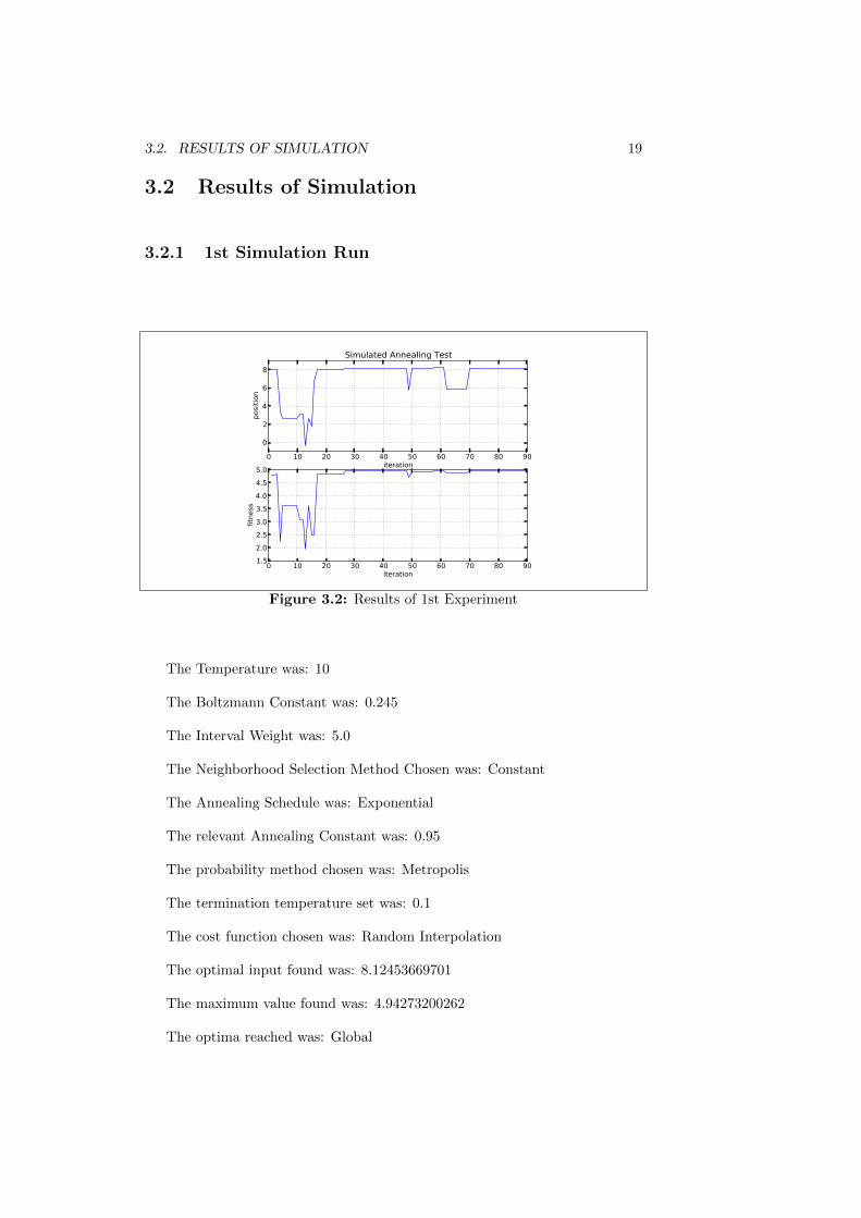
3.2.1 1st Simulation Run
0 10 20 30 40 50 60 70 80 90iteration
0
2
4
6
8
posi
tion
Simulated Annealing Test
0 10 20 30 40 50 60 70 80 90iteration
1.5
2.0
2.5
3.0
3.5
4.0
4.5
5.0
fitn
ess
Figure 3.2: Results of 1st Experiment
The Temperature was: 10
The Boltzmann Constant was: 0.245
The Interval Weight was: 5.0
The Neighborhood Selection Method Chosen was: Constant
The Annealing Schedule was: Exponential
The relevant Annealing Constant was: 0.95
The probability method chosen was: Metropolis
The termination temperature set was: 0.1
The cost function chosen was: Random Interpolation
The optimal input found was: 8.12453669701
The maximum value found was: 4.94273200262
The optima reached was: Global

20 CHAPTER 3. RESULTS
3.2.2 2nd Simulation Run
0 10 20 30 40 50 60 70 80iteration
2
3
4
5
6
7
8
9
posi
tion
Simulated Annealing Test
0 10 20 30 40 50 60 70 80iteration
1.5
2.0
2.5
3.0
3.5
4.0
4.5
5.0
fitn
ess
Figure 3.3: Results of 2nd Experiment
The Temperature was: 5
The Boltzmann Constant was: 0.245
The Interval Weight was: 5.0
The Neighborhood Selection Method Chosen was: Constant
The Annealing Schedule was: Exponential
The relevant Annealing Constant was: 0.95
The probability method chosen was: Metropolis
The termination temperature set was: 0.1
The cost function chosen was: Random Interpolation
The optimal input found was: 8.25702992337
The maximum value found was: 4.94262557569
The optima reached was: Global

3.2. RESULTS OF SIMULATION 21
3.2.3 3rd Simulation Run
0 10 20 30 40 50 60 70 80 90iteration
6
4
2
0
2
4
6
posi
tion
Simulated Annealing Test
0 10 20 30 40 50 60 70 80 90iteration
0
1
2
3
4
5
fitn
ess
Figure 3.4: Results of 3rd Experiment
The Temperature was: 10
The Boltzmann Constant was: 0.245
The Interval Weight was: 0.4
The Neighborhood Selection Method Chosen was: Square Root
The Annealing Schedule was: Exponential
The relevant Annealing Constant was: 0.95
The probability method chosen was: Metropolis
The termination temperature set was: 0.1
The cost function chosen was: Random Interpolation
The optimal input found was: -3.94145196297
The maximum value found was: 4.72607762918
The optima reached was: Local

22 CHAPTER 3. RESULTS
3.2.4 4th Simulation Run
0 10 20 30 40 50 60 70 80iteration
4.5
4.0
3.5
3.0
2.5
2.0
1.5posi
tion
Simulated Annealing Test
0 10 20 30 40 50 60 70 80iteration
2.0
2.5
3.0
3.5
4.0
4.5
5.0
fitn
ess
Figure 3.5: Results of 4th Experiment
The Temperature was: 5
The Boltzmann Constant was: 0.245
The Interval Weight was: 0.2
The Neighborhood Selection Method Chosen was: Square Root
The Annealing Schedule was: Exponential
The relevant Annealing Constant was: 0.95
The probability method chosen was: Metropolis
The termination temperature set was: 0.1
The cost function chosen was: Random Interpolation
The optimal input found was: -3.91731183007
The maximum value found was: 4.72582418859
The optima reached was: Local

3.2. RESULTS OF SIMULATION 23
3.2.5 5th Simulation Run
0 5 10 15 20 25 30 35 40 45iteration
6.0
6.5
7.0
7.5
8.0
8.5
posi
tion
Simulated Annealing Test
0 5 10 15 20 25 30 35 40 45iteration
4.82
4.84
4.86
4.88
4.90
4.92
4.94
4.96
4.98
fitn
ess
Figure 3.6: Results of 5th Experiment
The Temperature was: 1
The Boltzmann Constant was: 0.245
The Interval Weight was: 0.04
The Neighborhood Selection Method Chosen was: Square Root
The Annealing Schedule was: Exponential
The relevant Annealing Constant was: 0.95
The probability method chosen was: Metropolis
The termination temperature set was: 0.1
The cost function chosen was: Random Interpolation
The optimal input found was: 8.36686935583
The maximum value found was: 4.83238399159
The optima reached was: Global

24 CHAPTER 3. RESULTS
3.2.6 6th Simulation Run
0 10 20 30 40 50 60 70 80 90iteration
10
5
0
5
10posi
tion
Simulated Annealing Test
0 10 20 30 40 50 60 70 80 90iteration
0.51.0
1.52.02.53.03.54.0
4.55.0
fitn
ess
Figure 3.7: Results of 6th Experiment
The Temperature was: 10
The Boltzmann Constant was: 0.245
The Interval Weight was: 0.04
The Neighborhood Selection Method Chosen was: Square Root
The Annealing Schedule was: Exponential
The relevant Annealing Constant was: 0.95
The probability method chosen was: Alternate
The termination temperature set was: 0.1
The cost function chosen was: Random Interpolation
The optimal input found was: 8.19310048306
The maximum value found was: 4.96191639881
The optima reached was: Global

3.2. RESULTS OF SIMULATION 25
3.2.7 7th Simulation Run
0 10 20 30 40 50 60 70 80iteration
12
34
56789
10
posi
tion
Simulated Annealing Test
0 10 20 30 40 50 60 70 80iteration
1.0
1.5
2.0
2.5
3.0
3.5
4.0
4.5
5.0
fitn
ess
Figure 3.8: Results of 7th Experiment
The Temperature was: 5
The Boltzmann Constant was: 0.245
The Interval Weight was: 0.02
The Neighborhood Selection Method Chosen was: Square Root
The Annealing Schedule was: Exponential
The relevant Annealing Constant was: 0.95
The probability method chosen was: Alternate
The termination temperature set was: 0.1
The cost function chosen was: Random Interpolation
The optimal input found was: 8.26344538045
The maximum value found was: 4.93879936195
The optima reached was: Global

26 CHAPTER 3. RESULTS
3.2.8 8th Simulation Run
0 5 10 15 20 25 30 35 40 45iteration
1
2
3
4
5
6
7
posi
tion
Simulated Annealing Test
0 5 10 15 20 25 30 35 40 45iteration
2.7
2.82.93.03.13.23.33.43.53.6
fitn
ess
Figure 3.9: Results of 8th Experiment
The Temperature was: 1
The Boltzmann Constant was: 0.245
The Interval Weight was: 0.04
The Neighborhood Selection Method Chosen was: Square Root
The Annealing Schedule was: Exponential
The relevant Annealing Constant was: 0.95
The probability method chosen was: Alternate
The termination temperature set was: 0.1
The cost function chosen was: Random Interpolation
The optimal input found was: 2.38064428537
The maximum value found was: 3.55647132056
The optima reached was: Local
3.2. RESULTS OF SIMULATION 27
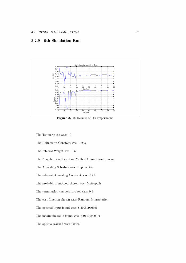
3.2.9 9th Simulation Run
0 10 20 30 40 50 60 70 80 90iteration
6.0
6.5
7.0
7.5
8.0
8.5
9.0
9.5
10.0
posi
tion
Simulated Annealing Test
0 10 20 30 40 50 60 70 80 90iteration
0.51.0
1.52.02.53.03.54.0
4.55.0
fitn
ess
Figure 3.10: Results of 9th Experiment
The Temperature was: 10
The Boltzmann Constant was: 0.245
The Interval Weight was: 0.5
The Neighborhood Selection Method Chosen was: Linear
The Annealing Schedule was: Exponential
The relevant Annealing Constant was: 0.95
The probability method chosen was: Metropolis
The termination temperature set was: 0.1
The cost function chosen was: Random Interpolation
The optimal input found was: 8.29950940596
The maximum value found was: 4.91110900971
The optima reached was: Global

28 CHAPTER 3. RESULTS
3.2.10 10th Simulation Run
0 10 20 30 40 50 60 70 80iteration
2.0
2.2
2.4
2.6
2.8
3.0
3.2
3.4
posi
tion
Simulated Annealing Test
0 10 20 30 40 50 60 70 80iteration
2.2
2.4
2.6
2.8
3.0
3.2
3.4
3.6
3.8
fitn
ess
Figure 3.11: Results of 10th Experiment
The Temperature was: 5
The Boltzmann Constant was: 0.245
The Interval Weight was: 1.0
The Neighborhood Selection Method Chosen was: Linear
The Annealing Schedule was: Exponential
The relevant Annealing Constant was: 0.95
The probability method chosen was: Metropolis
The termination temperature set was: 0.1
The cost function chosen was: Random Interpolation
The optimal input found was: 2.50249440476
The maximum value found was: 3.6303864234
The optima reached was: Local
3.2. RESULTS OF SIMULATION 29
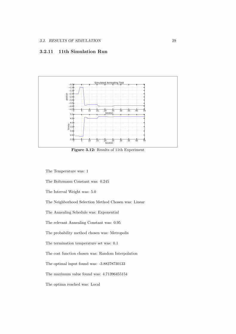
3.2.11 11th Simulation Run
0 5 10 15 20 25 30 35 40 45iteration
4.5
4.0
3.5
3.0
2.5
2.0
1.5
1.0
0.5
posi
tion
Simulated Annealing Test
0 5 10 15 20 25 30 35 40 45iteration
2.0
2.5
3.0
3.5
4.0
4.5
5.0
fitn
ess
Figure 3.12: Results of 11th Experiment
The Temperature was: 1
The Boltzmann Constant was: 0.245
The Interval Weight was: 5.0
The Neighborhood Selection Method Chosen was: Linear
The Annealing Schedule was: Exponential
The relevant Annealing Constant was: 0.95
The probability method chosen was: Metropolis
The termination temperature set was: 0.1
The cost function chosen was: Random Interpolation
The optimal input found was: -3.88278730133
The maximum value found was: 4.71396455154
The optima reached was: Local

30 CHAPTER 3. RESULTS
3.2.12 12th Simulation Run
0 10 20 30 40 50 60 70 80 90iteration
3
4
5
6
7
8
9
10
posi
tion
Simulated Annealing Test
0 10 20 30 40 50 60 70 80 90iteration
1.0
1.5
2.0
2.5
3.0
3.5
4.0
4.5
5.0
fitn
ess
Figure 3.13: Results of 12th Experiment
The Temperature was: 10
The Boltzmann Constant was: 0.245
The Interval Weight was: 0.5
The Neighborhood Selection Method Chosen was: Linear
The Annealing Schedule was: Exponential
The relevant Annealing Constant was: 0.95
The probability method chosen was: Alternate
The termination temperature set was: 0.1
The cost function chosen was: Random Interpolation
The optimal input found was: 8.24916033885
The maximum value found was: 4.9468572584
The optima reached was: Global

3.2. RESULTS OF SIMULATION 31
3.2.13 13th Simulation Run
0 10 20 30 40 50 60 70 80iteration
5.0
5.5
6.0
6.5
7.0
7.5
8.0
posi
tion
Simulated Annealing Test
0 10 20 30 40 50 60 70 80iteration
2.0
2.5
3.0
3.5
4.0
4.5
5.0
fitn
ess
Figure 3.14: Results of 13th Experiment
The Temperature was: 5
The Boltzmann Constant was: 0.245
The Interval Weight was: 1.0
The Neighborhood Selection Method Chosen was: Linear
The Annealing Schedule was: Exponential
The relevant Annealing Constant was: 0.95
The probability method chosen was: Alternate
The termination temperature set was: 0.1
The cost function chosen was: Random Interpolation
The optimal input found was: 5.99006003943
The maximum value found was: 4.84934812591
The optima reached was: Local

32 CHAPTER 3. RESULTS
3.2.14 14th Simulation Run
0 5 10 15 20 25 30 35 40 45iteration
2.5
3.0
3.5
4.0
4.5
5.0
5.5
6.0
posi
tion
Simulated Annealing Test
0 5 10 15 20 25 30 35 40 45iteration
3.6
3.8
4.0
4.2
4.4
4.6
4.8
5.0
fitn
ess
Figure 3.15: Results of 14th Experiment
The Temperature was: 1
The Boltzmann Constant was: 0.245
The Interval Weight was: 5.0
The Neighborhood Selection Method Chosen was: Linear
The Annealing Schedule was: Exponential
The relevant Annealing Constant was: 0.95
The probability method chosen was: Alternate
The termination temperature set was: 0.1
The cost function chosen was: Random Interpolation
The optimal input found was: 5.81446248631
The maximum value found was: 4.84908964862
The optima reached was: Local

3.2. RESULTS OF SIMULATION 33
3.2.15 15th Simulation Run
0 10 20 30 40 50 60 70 80 90iteration
10
5
0
5
10
posi
tion
Simulated Annealing Test
0 10 20 30 40 50 60 70 80 90iteration
2.0
2.5
3.0
3.5
4.0
4.5
5.0
fitn
ess
Figure 3.16: Results of 15th Experiment
The Temperature was: 10
The Boltzmann Constant was: 0.245
The Interval Weight was: 0.05
The Neighborhood Selection Method Chosen was: Squared
The Annealing Schedule was: Exponential
The relevant Annealing Constant was: 0.95
The probability method chosen was: Metropolis
The termination temperature set was: 0.1
The cost function chosen was: Random Interpolation
The optimal input found was: 8.17734638299
The maximum value found was: 4.96125587134
The optima reached was: Global

34 CHAPTER 3. RESULTS
3.2.16 16th Simulation Run
0 10 20 30 40 50 60 70 80iteration
10
5
0
5
10posi
tion
Simulated Annealing Test
0 10 20 30 40 50 60 70 80iteration
2.0
2.5
3.0
3.5
4.0
4.5
5.0
fitn
ess
Figure 3.17: Results of 16th Experiment
The Temperature was: 5
The Boltzmann Constant was: 0.245
The Interval Weight was: 0.2
The Neighborhood Selection Method Chosen was: Squared
The Annealing Schedule was: Exponential
The relevant Annealing Constant was: 0.95
The probability method chosen was: Metropolis
The termination temperature set was: 0.1
The cost function chosen was: Random Interpolation
The optimal input found was: 5.92454497566
The maximum value found was: 4.88964836538
The optima reached was: Local

3.2. RESULTS OF SIMULATION 35
3.2.17 17th Simulation Run
0 5 10 15 20 25 30 35 40 45iteration
3.55
3.60
3.65
3.70
3.75
3.80
3.85
3.90
posi
tion
Simulated Annealing Test
0 5 10 15 20 25 30 35 40 45iteration
1.0
1.1
1.2
1.3
1.4
1.5
1.6
1.7
1.8
fitn
ess
Figure 3.18: Results of 17th Experiment
The Temperature was: 1
The Boltzmann Constant was: 0.245
The Interval Weight was: 5.0
The Neighborhood Selection Method Chosen was: Squared
The Annealing Schedule was: Exponential
The relevant Annealing Constant was: 0.95
The probability method chosen was: Metropolis
The termination temperature set was: 0.1
The cost function chosen was: Random Interpolation
The optimal input found was: 3.63840734657
The maximum value found was: 1.59143401283
The optima reached was: Nonoptimal

36 CHAPTER 3. RESULTS
3.2.18 18th Simulation Run
0 10 20 30 40 50 60 70 80 90iteration
10
5
0
5
10posi
tion
Simulated Annealing Test
0 10 20 30 40 50 60 70 80 90iteration
1.5
2.0
2.5
3.0
3.5
4.0
4.5
5.0
fitn
ess
Figure 3.19: Results of 18th Experiment
The Temperature was: 10
The Boltzmann Constant was: 0.245
The Interval Weight was: 0.05
The Neighborhood Selection Method Chosen was: Squared
The Annealing Schedule was: Exponential
The relevant Annealing Constant was: 0.95
The probability method chosen was: Alternate
The termination temperature set was: 0.1
The cost function chosen was: Random Interpolation
The optimal input found was: 5.84291572758
The maximum value found was: 4.87167478904
The optima reached was: Local

3.2. RESULTS OF SIMULATION 37
3.2.19 19th Simulation Run
0 10 20 30 40 50 60 70 80iteration
10
5
0
5
10
posi
tion
Simulated Annealing Test
0 10 20 30 40 50 60 70 80iteration
2.5
3.0
3.5
4.0
4.5
fitn
ess
Figure 3.20: Results of 19th Experiment
The Temperature was: 5
The Boltzmann Constant was: 0.245
The Interval Weight was: 0.2
The Neighborhood Selection Method Chosen was: Squared
The Annealing Schedule was: Exponential
The relevant Annealing Constant was: 0.95
The probability method chosen was: Alternate
The termination temperature set was: 0.1
The cost function chosen was: Random Interpolation
The optimal input found was: -9.04789162475
The maximum value found was: 4.25423352425
The optima reached was: Local

38 CHAPTER 3. RESULTS
3.2.20 20th Simulation Run
0 5 10 15 20 25 30 35 40 45iteration
4.95
5.00
5.05
5.10
5.15
5.20
5.25posi
tion
Simulated Annealing Test
0 5 10 15 20 25 30 35 40 45iteration
2.2
2.32.4
2.52.62.7
2.82.93.03.1
fitn
ess
Figure 3.21: Results of 20th Experiment
The Temperature was: 1
The Boltzmann Constant was: 0.245
The Interval Weight was: 5.0
The Neighborhood Selection Method Chosen was: Squared
The Annealing Schedule was: Exponential
The relevant Annealing Constant was: 0.95
The probability method chosen was: Alternate
The termination temperature set was: 0.1
The cost function chosen was: Random Interpolation
The optimal input found was: 5.17406360604
The maximum value found was: 2.96278314043
The optima reached was: Local

3.2. RESULTS OF SIMULATION 39
3.2.21 21st Simulation Run
0 10 20 30 40 50 60 70 80 90iteration
10
5
0
5
10
posi
tion
Simulated Annealing Test
0 10 20 30 40 50 60 70 80 90iteration
0.51.0
1.52.02.53.03.54.0
4.55.0
fitn
ess
Figure 3.22: Results of 21st Experiment
The Temperature was: 10
The Boltzmann Constant was: 0.245
The Interval Weight was: 5.5
The Neighborhood Selection Method Chosen was: Exponential
The Annealing Schedule was: Exponential
The relevant Annealing Constant was: 0.95
The probability method chosen was: Metropolis
The termination temperature set was: 0.1
The cost function chosen was: Random Interpolation
The optimal input found was: 5.8349624473
The maximum value found was: 4.8661724921
The optima reached was: Local

40 CHAPTER 3. RESULTS
3.2.22 22nd Simulation Run
0 10 20 30 40 50 60 70 80iteration
8
7
6
5
4
3
2
posi
tion
Simulated Annealing Test
0 10 20 30 40 50 60 70 80iteration
1.5
2.0
2.5
3.0
3.5
4.0
4.5
5.0
fitn
ess
Figure 3.23: Results of 22nd Experiment
The Temperature was: 5
The Boltzmann Constant was: 0.245
The Interval Weight was: 6.1
The Neighborhood Selection Method Chosen was: Exponential
The Annealing Schedule was: Exponential
The relevant Annealing Constant was: 0.95
The probability method chosen was: Metropolis
The termination temperature set was: 0.1
The cost function chosen was: Random Interpolation
The optimal input found was: -4.02034824486
The maximum value found was: 4.67704142695
The optima reached was: Local

3.2. RESULTS OF SIMULATION 41
3.2.23 23rd Simulation Run
0 5 10 15 20 25 30 35 40 45iteration
2.2
2.3
2.4
2.5
2.6
2.7
2.8
2.9
posi
tion
Simulated Annealing Test
0 5 10 15 20 25 30 35 40 45iteration
3.40
3.45
3.50
3.55
3.60
3.65
fitn
ess
Figure 3.24: Results of 23rd Experiment
The Temperature was: 1
The Boltzmann Constant was: 0.245
The Interval Weight was: 13.6
The Neighborhood Selection Method Chosen was: Exponential
The Annealing Schedule was: Exponential
The relevant Annealing Constant was: 0.95
The probability method chosen was: Metropolis
The termination temperature set was: 0.1
The cost function chosen was: Random Interpolation
The optimal input found was: 2.54326998373
The maximum value found was: 3.64055218711
The optima reached was: Local

42 CHAPTER 3. RESULTS
3.2.24 24th Simulation Run
0 10 20 30 40 50 60 70 80 90iteration
5
4
3
2
1
0
1
2
3
posi
tion
Simulated Annealing Test
0 10 20 30 40 50 60 70 80 90iteration
1.0
1.5
2.0
2.5
3.0
3.5
4.0
4.5
5.0
fitn
ess
Figure 3.25: Results of 24th Experiment
The Temperature was: 10
The Boltzmann Constant was: 0.245
The Interval Weight was: 5.5
The Neighborhood Selection Method Chosen was: Exponential
The Annealing Schedule was: Exponential
The relevant Annealing Constant was: 0.95
The probability method chosen was: Alternate
The termination temperature set was: 0.1
The cost function chosen was: Random Interpolation
The optimal input found was: -3.78353911027
The maximum value found was: 4.61158829596
The optima reached was: Local

3.2. RESULTS OF SIMULATION 43
3.2.25 25th Simulation Run
0 10 20 30 40 50 60 70 80iteration
3
4
5
6
7
8
9
posi
tion
Simulated Annealing Test
0 10 20 30 40 50 60 70 80iteration
1.5
2.0
2.5
3.0
3.5
4.0
4.5
5.0
fitn
ess
Figure 3.26: Results of 25th Experiment
The Temperature was: 5
The Boltzmann Constant was: 0.245
The Interval Weight was: 6.1
The Neighborhood Selection Method Chosen was: Exponential
The Annealing Schedule was: Exponential
The relevant Annealing Constant was: 0.95
The probability method chosen was: Alternate
The termination temperature set was: 0.1
The cost function chosen was: Random Interpolation
The optimal input found was: 8.290748868
The maximum value found was: 4.91878894657
The optima reached was: Global

44 CHAPTER 3. RESULTS
3.2.26 26th Simulation Run
0 5 10 15 20 25 30 35 40 45iteration
6.0
6.5
7.0
7.5
8.0
8.5
9.0
posi
tion
Simulated Annealing Test
0 5 10 15 20 25 30 35 40 45iteration
3.6
3.8
4.0
4.2
4.4
4.6
4.8
5.0
fitn
ess
Figure 3.27: Results of 26th Experiment
The Temperature was: 1
The Boltzmann Constant was: 0.245
The Interval Weight was: 13.6
The Neighborhood Selection Method Chosen was: Exponential
The Annealing Schedule was: Exponential
The relevant Annealing Constant was: 0.95
The probability method chosen was: Alternate
The termination temperature set was: 0.1
The cost function chosen was: Random Interpolation
The optimal input found was: 8.26080563276
The maximum value found was: 4.94041449576
The optima reached was: Global

3.2. RESULTS OF SIMULATION 45
3.2.27 27th Simulation Run
0 10 20 30 40 50 60 70 80 90iteration
10
5
0
5
10
posi
tion
Simulated Annealing Test
0 10 20 30 40 50 60 70 80 90iteration
0.51.0
1.52.02.53.03.54.0
4.55.0
fitn
ess
Figure 3.28: Results of 27th Experiment
The Temperature was: 10
The Boltzmann Constant was: 0.245
The Interval Weight was: 127.0
The Neighborhood Selection Method Chosen was: Normal Distribution
The Annealing Schedule was: Exponential
The relevant Annealing Constant was: 0.95
The probability method chosen was: Alternate
The termination temperature set was: 0.1
The cost function chosen was: Random Interpolation
The optimal input found was: 6.03075787558
The maximum value found was: 4.7978270401
The optima reached was: Local

46 CHAPTER 3. RESULTS
3.2.28 28th Simulation Run
0 10 20 30 40 50 60 70 80iteration
10
5
0
5
10posi
tion
Simulated Annealing Test
0 10 20 30 40 50 60 70 80iteration
0
1
2
3
4
5
fitn
ess
Figure 3.29: Results of 28th Experiment
The Temperature was: 5
The Boltzmann Constant was: 0.245
The Interval Weight was: 63.6
The Neighborhood Selection Method Chosen was: Normal Distribution
The Annealing Schedule was: Exponential
The relevant Annealing Constant was: 0.95
The probability method chosen was: Alternate
The termination temperature set was: 0.1
The cost function chosen was: Random Interpolation
The optimal input found was: 8.12612264053
The maximum value found was: 4.94366208577
The optima reached was: Global

3.2. RESULTS OF SIMULATION 47
3.2.29 29th Simulation Run
0 5 10 15 20 25 30 35 40 45iteration
5.65
5.70
5.75
5.80
5.85
5.90
5.95
6.00
6.05
posi
tion
Simulated Annealing Test
0 5 10 15 20 25 30 35 40 45iteration
4.60
4.65
4.70
4.75
4.80
4.85
4.90
fitn
ess
Figure 3.30: Results of 29th Experiment
The Temperature was: 1
The Boltzmann Constant was: 0.245
The Interval Weight was: 20.7
The Neighborhood Selection Method Chosen was: Normal Distribution
The Annealing Schedule was: Exponential
The relevant Annealing Constant was: 0.95
The probability method chosen was: Alternate
The termination temperature set was: 0.1
The cost function chosen was: Random Interpolation
The optimal input found was: 5.74795311155
The maximum value found was: 4.76635076685
The optima reached was: Local

48 CHAPTER 3. RESULTS
3.2.30 30th Simulation Run
0 10 20 30 40 50 60 70 80 90iteration
8642
02
468
10
posi
tion
Simulated Annealing Test
0 10 20 30 40 50 60 70 80 90iteration
0
1
2
3
4
5
fitn
ess
Figure 3.31: Results of 30th Experiment
The Temperature was: 10
The Boltzmann Constant was: 0.245
The Interval Weight was: 127.0
The Neighborhood Selection Method Chosen was: Normal Distribution
The Annealing Schedule was: Exponential
The relevant Annealing Constant was: 0.95
The probability method chosen was: Metropolis
The termination temperature set was: 0.1
The cost function chosen was: Random Interpolation
The optimal input found was: 6.10503840733
The maximum value found was: 4.65468377356
The optima reached was: Local

3.2. RESULTS OF SIMULATION 49
3.2.31 31st Simulation Run
0 10 20 30 40 50 60 70 80iteration
10
5
0
5
10
posi
tion
Simulated Annealing Test
0 10 20 30 40 50 60 70 80iteration
2.0
2.5
3.0
3.5
4.0
4.5
5.0
fitn
ess
Figure 3.32: Results of 31st Experiment
The Temperature was: 5
The Boltzmann Constant was: 0.245
The Interval Weight was: 63.6
The Neighborhood Selection Method Chosen was: Normal Distribution
The Annealing Schedule was: Exponential
The relevant Annealing Constant was: 0.95
The probability method chosen was: Metropolis
The termination temperature set was: 0.1
The cost function chosen was: Random Interpolation
The optimal input found was: 8.06337249662
The maximum value found was: 4.8885707594
The optima reached was: Global

50 CHAPTER 3. RESULTS
3.2.32 32nd Simulation Run
0 5 10 15 20 25 30 35 40 45iteration
4.00
3.98
3.96
3.94
3.92
3.90
3.88
3.86
3.84posi
tion
Simulated Annealing Test
0 5 10 15 20 25 30 35 40 45iteration
4.69
4.70
4.71
4.72
4.73
fitn
ess
Figure 3.33: Results of 32nd Experiment
The Temperature was: 1
The Boltzmann Constant was: 0.245
The Interval Weight was: 20.7
The Neighborhood Selection Method Chosen was: Normal Distribution
The Annealing Schedule was: Exponential
The relevant Annealing Constant was: 0.95
The probability method chosen was: Metropolis
The termination temperature set was: 0.1
The cost function chosen was: Random Interpolation
The optimal input found was: -3.95033095606
The maximum value found was: 4.72443970661
The optima reached was: Local

3.3. GENERAL REMARKS ON SIMULATION RESULTS 51
3.3 General Remarks on Simulation Results
The only thing that needs to be determined for the analysis of these simulationresults is whether or not the run converges on the global maximum, on one ofthe local maxima, or if it did not converge at all. Of these, only the 17th runof the simulation did not converge to an optimal solution. This suggests thatfor the given conditions of that particular run that convergence to an optimalsolution is unlikely.
For the rest, it seems that for higher temperatures that the algorithm islikely to converge on the global optimum independent of the other choices thatare made. This suggests that temperature is the most important factor, alongwith the termination condition, in determining whether or not the algorithmwill converge on the global maximum.
In addition, it was determined that the selection method for determining theneighborhood that grew as a function of temperature (called the Normal Dis-tribution method in the algorithm) converged to the global maximum the leastoften. This motivated the abandoning of this neighborhood selection method inthe physical experiment algorithm.
3.4 Results of Physical Experiment
The algorithm that was written in Appendix B, with the corresponding modulefor interaction with the Arduino defined in Appendix C, was used to obtain oneset of results for the physical experiment. The graphs showing the selection ofthe method are shown after the logfile. The logfile from this experiment is:
These were the selections made for this experiment:The Neighborhood Selection Method Chosen was: Square RootThe probability method chosen was: MetropolisThe number of pulses per pulse train was: 5The number of experiments ran was: 1The number of points of data the Arduino collected was: 20For the 1st experiment, the optimal timing for the 1st element of the sequence
is: 1508The corresponding maximum voltage attained for this is: 0.9814453125For the 1st experiment, the optimal timing for the 2nd element of the se-
quence is: 3983The corresponding maximum voltage attained for this is: 0.9716796875For the 1st experiment, the optimal timing for the 3rd element of the se-
quence is: 2254The corresponding maximum voltage attained for this is: 0.83984375For the 1st experiment, the optimal timing for the 4th element of the se-
quence is: 3984The corresponding maximum voltage attained for this is: 0.8642578125For the 1st experiment, the optimal timing for the 5th element of the se-
quence is: 691The corresponding maximum voltage attained for this is: 0.8837890625For the 1st experiment, the optimal pulse train was: [1508, 3983, 2254, 3984,
691]The corresponding fitness for this pulse train was: 0.8837890625

52 CHAPTER 3. RESULTS
0 10 20 30 40 50 60 70 80 90iteration
0
500
1000
1500
2000
2500
3000
3500
4000
posi
tion
Slection process of element1
0 10 20 30 40 50 60 70 80 90iteration
0.0
0.2
0.4
0.6
0.8
1.0
fitn
ess
Figure 3.34: 1st pulse timing selection
0 10 20 30 40 50 60 70 80 90iteration
2500
3000
3500
4000
4500
5000
5500
6000
posi
tion
Slection process of element2
0 10 20 30 40 50 60 70 80 90iteration
0.0
0.2
0.4
0.6
0.8
1.0
fitn
ess
Figure 3.35: 2nd pulse timing selection

3.4. RESULTS OF PHYSICAL EXPERIMENT 53
0 10 20 30 40 50 60 70 80 90iteration
0
1000
2000
3000
4000
5000
6000
posi
tion
Slection process of element3
0 10 20 30 40 50 60 70 80 90iteration
0.0
0.2
0.4
0.6
0.8
1.0
fitn
ess
Figure 3.36: 3rd pulse timing selection
0 10 20 30 40 50 60 70 80 90iteration
0
1000
2000
3000
4000
5000
6000
posi
tion
Slection process of element4
0 10 20 30 40 50 60 70 80 90iteration
0.00.10.20.30.40.50.60.70.80.9
fitn
ess
Figure 3.37: 4th pulse timing selection

54 CHAPTER 3. RESULTS
0 10 20 30 40 50 60 70 80 90iteration
0
1000
2000
3000
4000
5000
posi
tion
Slection process of element5
0 10 20 30 40 50 60 70 80 90iteration
0.0
0.2
0.4
0.6
0.8
1.0
fitn
ess
Figure 3.38: 5th pulse timing selection
3.5 Analysis of Physical Experiment
For this experiment, the voltage was taken across the resistor. This means thatthe voltage as a function of time is related to the first derivative of charge, whichmeans that the voltage behaves as a sine function allowing for our assumptionsabout when the optimal time occurrs to be true. In addition, it can also beassumed that there is no significant loss of charge from when the last pulse wasdelivered to the system and when the measurement of the amplitude was taken.Therefore, the charge after the previous pulse is assumed to be the charge presentwhen the voltage measurement was taken. We can use the established equationsin the Motivation section (specifically 1.35 and 1.36) in order to determine whatthe charge is for that moment in time. From there we can obtain the electricpotential as a function of charge, and this can be used to find the potentialenergy function for the LRC.
Using the Mathematica code in Appendix E with the results from this ex-periment, a fit for the electric potential is obtained in Figure 3.39.
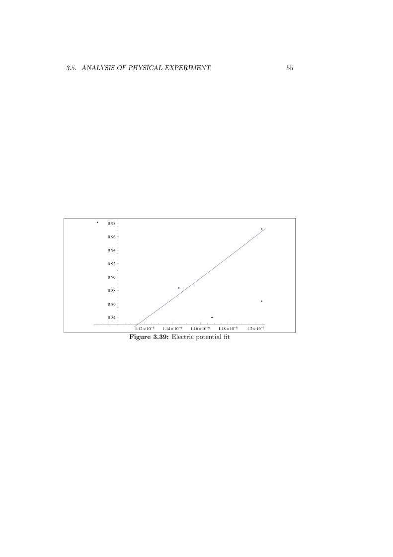
3.5. ANALYSIS OF PHYSICAL EXPERIMENT 55
Figure 3.39: Electric potential fit

56 CHAPTER 3. RESULTS

Chapter 4
Discussion
4.1 Conclusions
The experiment did perform within expectations. Either the solutions convergedto a timing near the optimal predicted timing of approximately 1000µs, theperiod of the oscillator, near some integer multiple of the optimal timing, or theywere in the vicinity of approaching such a timing as can be seen in the graphin Figure 4.1. This demonstrates that, with some further iterations includedin the algorithm, the algorithm is capable of approaching optimal solutions forphysical systems.
0.001 0.002 0.003 0.004
-1.0
-0.5
0.5
1.0
1.5
Figure 4.1: Plot of voltage for this LRC
However, this particular version of the experiment did not perform well atobtaining the necessary data for finding a fit for the potential energy. Thecharge data acquired from the timing was not good for determining a potentialfit for this experiment. However, because we can obtain fitness amplitude mea-surements using this methodology there is still potential for this methodologyto find the potential energy function if the timing can be assessed properly.
57

58 CHAPTER 4. DISCUSSION
4.2 Next Steps With this Methodology
Some of the next steps with this particular methodology would be to test thevarious combinations of neighborhood selection and selection probability as wasdone in the simulations. Then it could be determined whether or not certainselections of this method are better or worse for this particular experiment.
In addition, this methodology either needs to be able to determine the timingat which a measurement was taken, or it needs to be applied to a differentoscillator. This timing information is critical to determining the potential energyfunction, especially with regards to determining the charge. If it turns outthat this particular experiment is not designed properly with regards to thisparticular oscillator, then it needs to be adjusted for a different oscillator. Oneexample of a different oscillator that could be used is with a magnetic pendulum,and instead of finding the current voltage the experiment could keep track ofthe angular position.
4.3 Future Directions
Future applications of a similar methodology would involve various other typesof oscillators that require different hardware and software capabilities, and forthis methodology to be used in conjunction with another optimization methodfor when this method alone does not suffice for a particular problem.
One of the future applications intended for this method is to use it to find anoptimal sequence of ultrafast laser pulses for exciting a particular crystal. Thesecrystals have potential energy functions associated with them that are currentlyunknown. However, this experiment can be used to find the potential energyfunction using an analysis process similar to what is outlined in the motivationsection.
However, for this particular problem sometimes it takes more than a few laserpulses before some sort of measurable oscillation happens. For this situation, itwould be more than appropriate to use a genetic algorithm to find the optimaltimings for the first few pulses. After that, this simulated annealing methodcan continue to build up the sequence pulse by pulse, allowing us to acquire theamplitude information after each pulse in the sequence afterwards. This willallow for us to determine the potential energy function of the crystal.

Appendix A
Simulated Annealing TestAlgorithm
1 from pylab import ∗ #For p l o t t i n g2 import math #For c a l l i n g var i ous f unc t i on s3 import random #For gene ra t i on o f pseudorandom numbers4 import numpy as np #Numerical l i b r a r y5 import s c ipy #S c i e n t i f i c computation l i b r a r y6 import s c ipy . i n t e r p o l a t e #For the i n t e r p o l a t i o n func t i on7 import matp lo t l i b . pyplot as p l t #Also f o r p l o t t i n g8 import csv #For the gene ra t i on o f . csv f i l e s9 import sys #For f i l e wr i t i ng
1011 ”””12 The f o l l ow i ng three l i n e s d e f i n e an i n t e r p o l a t i n g func t i on over
the range13 −10 to 10 . The i n t e r p o l a t i o n method i s 1D cubic , and t h i s func t i on
cannot14 be eva luated out s id e o f the bounds .15 ”””16 in t e rpo l a t i onX = [−10.0 , −9.0 , −8.0 , −7.0 , −6.0 , −5.0 , −4.0 , −3.0 ,
−2.0 , −1.0 , 0 . 0 , 1 . 0 , 2 . 0 , 3 . 0 , 4 . 0 , 5 . 0 , 6 . 0 , 7 . 0 , 8 . 0 , 9 . 0 ,1 0 . 0 ]
17 in t e rpo l a t i onY = [1 .4125429788401118 , 4 .2303586635432469 ,2 .9150883719169718 , 2 .4927172814567351 , 1 .0656216430970016 ,0 .96046262410472871 , 4 .6972935801324649 , 2 .3895126263029107 ,2 .3922138420600785 , 2 .3834152342501835 , 1 .4678720026242216 ,0 .21532145496108546 , 2 .9089386977089138 , 3 .2503152700752054 ,0 .87631644883654436 , 2 .3113950122881244 , 4 .8386630886391035 ,1 .9046074692601027 , 4 .7934041954114956 , 2 .8450389093210138 ,1 .3939939155628545 ]
18 in t e rpo la t edFunct i on = sc ipy . i n t e r p o l a t e . in te rp1d ( inte rpo la t i onX ,in te rpo la t i onY , kind=’ cubic ’ , bounds er ror=True )
192021 ”””22 The f o l l ow i ng de f commands e s t a b l i s h a s e t o f u s e f u l f un c t i on s23 f o r the s imulated annea l ing a lgor i thm .24 ”””25 #Def ine s the Boltzmann d i s t rubut i on func t i on f o r va r i ous
p r obab i l i t y computations26 de f boltzmann (x , y ,T, k ) :27 d i f f e r e n c e = y − x
59

60 APPENDIX A. SIMULATED ANNEALING TEST ALGORITHM
28 d i v i s o r = k ∗ T29 p = f l o a t ( d i f f e r e n c e ) / f l o a t ( d i v i s o r )30 p r obab i l i t y = math . exp (p)31 re turn p r obab i l i t y3233 #Def ine s the p r obab i l i t y func t i on from the standard Metropo l i s
a lgor i thm34 de f prob1 (x , y ,T, k ) :35 i f x < y :36 re turn 137 e l s e :38 a = boltzmann (x , y ,T, k )39 re turn a4041 ”””42 This d e f i n e s an a l t e r n a t e p r obab i l i t y func t i on where be t t e r
gue s s e s are kept43 most o f the time , but not a l l o f the time . This p r obab i l i t y f o r
the be t t e r44 gue s s e s i s equal to one minus the p r obab i l i t y o f keeping a worse
guess that45 has the same d i f f e r e n c e in f i t n e s s from the cur rent bes t guess .46 ”””47 de f prob2 (x , y ,T, k ) :48 i f x < y :49 a = boltzmann (y , x ,T, k )50 a = 1−a51 re turn a52 e l s e :53 a = boltzmann (x , y ,T, k )54 re turn a5556 #Allows the user to choose which p r obab i l i t y func t i on w i l l be used
during the round57 de f prob (x , y ,T, k , cho i c e ) :58 i f ( cho i c e == ’ Metropo l i s ’ ) :59 p = prob1 (x , y ,T, k )60 re turn p61 e l i f ( cho i c e == ’ Al te rnate ’ ) :62 p = prob2 (x , y ,T, k )63 re turn p6465 #Gaussian f i t n e s s func t i on f o r t e s t s i nvo l v i ng a s i n g l e maximum66 de f f 1 ( x ) :67 p = math . pow(x , 2 )68 p = −p69 p = p / 2570 f i t = math . exp (p)71 re turn f i t7273 #The above i n t e r p o l a t ed func t i on i s c a l l e d f o r t e s t s i nvo l v i ng
mu l t ip l e maxima74 de f f 2 ( x ) :75 f i t = in t e rpo la t edFunct i on (x )76 f i t = f l o a t ( f i t )77 re turn f i t7879 #Lets the user s e l e c t the f i t n e s s func t i on f o r a g iven run80 de f f (x , cho i c e ) :81 i f ( cho i c e == ’ Gaussian ’ ) :82 f i t = f1 (x )83 re turn f i t
61
84 e l i f ( cho i c e == ’Random In t e r p o l a t i o n ’ ) :85 f i t = f2 (x )86 re turn f i t8788 #Square root neighbourhood s e l e c t i o n method89 de f l im i tF inde r1 (T,m) :90 a = T / m91 a = math . s q r t ( a )92 re turn a9394 #Linear neighbourhood s e l e c t i o n method95 de f l im i tF inde r2 (T,m) :96 a = m ∗ T97 return a9899 #Squared neighbourhood s e l e c t i o n method
100 de f l im i tF inde r3 (T,m) :101 a = T ∗ T102 a = a / m103 return a104105 #Exponent ia l neighbourhood s e l e c t i o n method106 de f l im i tF inde r4 (T,m) :107 a = 1 / T108 a = math . exp(−a )109 a = m ∗ a110 re turn a111112 #Normal d i s t r i b u t i o n neighbourhood s e l e c t i o n method113 de f l im i tF inde r5 (T,m) :114 a = 2 ∗ T ∗ T115 a = 1 / a116 a = math . exp(−a )117 tau = 2 ∗ pi118 s = math . s q r t ( tau )119 s = T ∗ s120 c = m / s121 a = a ∗ c122 re turn a123124 #Allows the user to s e l e c t which neighbourhood s e l e c t i o n method to
use125 de f l im i tF inde r (T,m, i n t e rva lCho i c e ) :126 i f ( i n t e rva lCho i c e == ’ Constant ’ ) :127 l im i t = m128 return l im i t129 e l i f ( i n t e rva lCho i c e == ’ Square Root ’ ) :130 l im i t = l im i tF inde r1 (T,m)131 re turn l im i t132 e l i f ( i n t e rva lCho i c e == ’ Linear ’ ) :133 l im i t = l im i tF inde r2 (T,m)134 re turn l im i t135 e l i f ( i n t e rva lCho i c e == ’ Squared ’ ) :136 l im i t = l im i tF inde r3 (T,m)137 re turn l im i t138 e l i f ( i n t e rva lCho i c e == ’ Exponent ia l ’ ) :139 l im i t = l im i tF inde r4 (T,m)140 re turn l im i t141 e l i f ( i n t e rva lCho i c e == ’Normal D i s t r i bu t i on ’ ) :142 l im i t = l im i tF inde r5 (T,m)143 re turn l im i t144

62 APPENDIX A. SIMULATED ANNEALING TEST ALGORITHM
145 #Generates a new guess that i s a ”mutation” o f the cur rent bes tguess
146 de f mutator (x , l im i t ) :147 whi le (True ) :148 whi l e (True ) :#Does not a l low a change o f 0149 change = random . uniform(− l im i t , l im i t )150 i f change != 0 :151 break152 new = f l o a t ( x ) + change153 i f (new < −10 or new > 10) :#Only gue s s e s with in the bounds
are chosen154 cont inue155 e l s e :156 break157 re turn new158159 #Allows the user to choose the annea l ing schedu le160 de f annealSchedule (T, const , cho i c e ) :161 i f ( cho i c e == ’ Exponent ia l ’ ) :#Exponent ia l annea l ing schedu le162 a = const ∗ T163 return a164 e l i f ( cho i c e == ’ Linear ’ ) :#Linear annea l ing schedu le165 a = T − const166 re turn a167168 p r i n t ”Set Temperature”169 T = raw input ( ) #The user s e t s the temperature at the beg inning o f
the run170 p r i n t ”Set Boltzmann Constant”171 k = raw input ( ) #The user s e t s the Boltzmann Constant f o r the
p r obab i l i t y d i s t r i b u t i o n func t i on172 p r i n t ”Set Neighbourhood Constant”173 m = raw input ( ) #The user s e t s the Neighbourhood Constant f o r a
g iven problem174 p r i n t ”Choose Neighbourhood S e l e c t i o n Method ( Constant , Square
Root , Linear , Squared , Exponent ia l or Normal D i s t r i bu t i on ) ”175 cho i c e = raw input ( ) #The user s e t s the neighbourhood s e l e c t i o n
method176 p r i n t ”Set Schedule Constant”177 scheduleConst = raw input ( ) #The user s e t s the constant f o r the
annea l ing schedu le178 p r i n t ”Choose Annealing Schedule ( Exponent ia l or Linear ) ”179 scheduleChoice = raw input ( ) #The user chooses the annea l ing
schedu le180 p r i n t ”Choose Probab i l i t y Method ( Metropo l i s or Al te rnate ) ”181 probChoice = raw input ( ) #The user chooses the s e l e c t i o n
p r obab i l i t y method182 p r i n t ”Choose F i tne s s Function ( Gaussian or Random In t e r p o l a t i o n ) ”183 f i tCho i c e = raw input ( ) #The user s e l e c t s which f i t n e s s func t i on
to exp lo r e184 p r i n t ”Set te rminat ion cond i t i on ”185 termin = raw input ( ) #The user s e t s the te rminat ion cond i t i on f o r
the a lgor i thm186 p r i n t ”Set f i l e names”187 fNameBase = raw input ( ) #The user s e t s the name base f o r the f i l e s
generated188189 #Conversion to appropr ia te types from raw input ( )190 T = f l o a t (T)191 k = f l o a t ( k )192 m = f l o a t (m)193 cho i c e = s t r ( cho i c e )

63
194 scheduleConst = f l o a t ( scheduleConst )195 scheduleChoice = s t r ( scheduleChoice )196 probChoice = s t r ( probChoice )197 f i tCho i c e = s t r ( f i tCho i c e )198 termin = f l o a t ( termin )199 fNameBase = s t r ( fNameBase )200 T i n i t i a l = T #Saves the i n i t i a l temperature f o r a l og f i l e201202 #I n i t i a l i z e s the f i g u r e203 f i g = p l t . f i g u r e ( )204 ax = f i g . add subplot (211)205 ay = f i g . add subplot (212)206 x , y , z = [ ] , [ ] , [ ] #Empty l i s t s f o r s t o r i n g data207 n=1 #Creates a counter208209 bestGuess = random . rand int (−10 ,10) #Makes a random in t e g e r guess
in the range210 be s tF i tn e s s = f ( bestGuess , f i tCho i c e ) #Computes the f i t n e s s211212 #The f o l l ow i n g i s the main s imulated annea l ing loop213 whi l e (T > termin ) : #Runs f o r as long as T i s g r e a t e r than the
te rminat ion cond i t i on214 l im = l im i tF inde r (T,m, cho i c e ) #Finds the l im i t s o f the
neighbourhood215 guess = mutator ( bestGuess , l im ) #Finds a new guess216 f i t n e s s = f ( guess , f i tCho i c e ) #Computes the new f i t n e s s217 #Computes the p r obab i l i t y o f keeping the guess218 maybeKeep = prob ( be s tF i tne s s , f i t n e s s ,T, k , probChoice )219 t e s t = random . random ( ) #Generates a random f l o a t from 0 to 1220 x . append (n) #Appends the cur rent count to the l i s t x221 i f (maybeKeep >= t e s t ) : #I f t h i s t e s t i s t rue we keep the new
guess222 y . append ( guess ) #Saves the guess to the l i s t y223 z . append ( f i t n e s s ) #Saves the f i t n e s s to the l i s t z224 bestGuess = guess #The new guess i s now the guess that i s
kept225 be s tF i tn e s s = f i t n e s s #The new f i t n e s s i s saved226 e l s e : #I f the t e s t was f a l s e we d i s r e ga rd the new guess227 y . append ( bestGuess ) #The cur rent bestGuess i s saved to y228 z . append ( be s tF i tn e s s ) #The cur rent b e s tF i tn e s s i s saved to
z229 n+=1 #Increments the count by 1230 #Changes the temperature in accordance with the annea l ing
schedu le231 T = annealSchedule (T, scheduleConst , scheduleChoice )232233 ”””234 The f o l l ow i ng gene ra t e s a . pdf with two graphs . The f i r s t graph
repre s en ted by the235 subplot ax i s a graph o f the guess with r e sp e c t to the i t e r a t i o n .
The second graph236 repre s en ted by the subplot ay i s a graph o f the f i t n e s s with
r e sp e c t to the i t e r a t i o n .237 ”””238 ax . p l o t (x , y )239 ax . g r id ( )240 ax . s e t x l a b e l ( ’ i t e r a t i o n ’ )241 ax . s e t y l a b e l ( ’ p o s i t i o n ’ )242 ay . p l o t (x , z )243 ay . g r id ( )244 ay . s e t x l a b e l ( ’ i t e r a t i o n ’ )245 ay . s e t y l a b e l ( ’ f i t n e s s ’ )

64 APPENDIX A. SIMULATED ANNEALING TEST ALGORITHM
246 ax . s e t t i t l e ( ’ Simulated Annealing Test ’ )247 graphName = fNameBase + ’ . pdf ’248 p l t . s a v e f i g ( graphName)249 #The f o l l ow i n g wr i t e s a . csv f i l e with the data f o r f u r t h e r
an a l y s i s in Mathematica i f so d e s i r ed250 dataLogName = fNameBase + ’ . csv ’251 with open (dataLogName , ’w ’ ) as da taF i l e :252 #This e s t a b i l i s h e s the formatt ing o f the . csv and how en t r i e s
are d iv ided253 dataWriter = csv . wr i t e r ( dataFi l e , d e l im i t e r=’ , ’ , quotechar=’ | ’
, quot ing=csv .QUOTEMINIMAL)254 c = 0255 #This names the columns o f the . csv256 dataWriter . writerow ( [ ’ I t e r a t i o n ’ , ’ Best Guess ’ , ’ F i tne s s ’ ] )257 whi le ( c < l en (y ) ) :258 #This grabs a l l e lements o f the l i s t s and wr i t e s them to
t h e i r259 #r e s p e c t i v e columns in the . csv260 gue s sS t r i ng = s t r ( y [ c ] )261 i t e r S t r i n g = s t r ( x [ c ] )262 f i t n e s s S t r i n g = s t r ( z [ c ] )263 dataWriter . writerow ( [ i t e r S t r i n g , gues sSt r ing , f i t n e s s S t r i n g
] )264 c+=1265266 #This shows the user the r e s u l t s o f the run and a l l ows the user to
wr i t e267 #commentary that w i l l be saved in the l o g f i l e268 p r i n t ”The optimal input f o r our co s t func t i on i s : ”269 p r i n t bestGuess270 p r i n t ”The optimal f i t n e s s i s : ”271 p r i n t b e s tF i tn e s s272 p r i n t ” State Commentary Here”273 Commentary = raw input ( )274 #Al l o f t h i s c r e a t e s the s t r i n g that w i l l be wr i t t en to the
l o g f i l e275 docStr ing = ’The Temperature was : ’276 docStr ing += s t r ( T i n i t i a l ) + ’ \n ’277 docStr ing += ’The Boltzmann Constant was : ’278 docStr ing += s t r ( k ) + ’ \n ’279 docStr ing += ’The Neighbourhood Constant was : ’280 docStr ing += s t r (m) + ’ \n ’281 docStr ing += ’The Neighbourhood S e l e c t i o n Method Chosen was : ’282 docStr ing += cho i c e + ’ \n ’283 docStr ing += ’The Annealing Schedule was : ’284 docStr ing += scheduleChoice + ’ \n ’285 docStr ing += ’The r e l e van t Annealing Constant was : ’286 docStr ing += s t r ( scheduleConst ) + ’ \n ’287 docStr ing += ’The p r obab i l i t y method chosen was : ’288 docStr ing += probChoice + ’ \n ’289 docStr ing += ’The terminat ion temperature s e t was : ’290 docStr ing += s t r ( termin ) + ’ \n ’291 docStr ing += ’The co s t func t i on chosen was : ’292 docStr ing += f i tCho i c e + ’ \n ’293 docStr ing += ’The optimal input found was : ’294 docStr ing += s t r ( bestGuess ) + ’ \n ’295 docStr ing += ’The maximum value found was : ’296 docStr ing += s t r ( b e s tF i t n e s s ) + ’ \n ’297 docStr ing += ’Commentary :\n ’298 docStr ing += s t r (Commentary )299 docFileName = fNameBase + ’ . txt ’300

65
301 #This wr i t e s the l o g f i l e302 with open ( docFileName , ’w ’ ) as l o gF i l e :303 l o gF i l e . wr i t e ( docStr ing )

66 APPENDIX A. SIMULATED ANNEALING TEST ALGORITHM

Appendix B
Main Experiment PythonCode
1 #Imports the nece s sa ry l i b r a r i e s2 import time3 #For pauses4 import s e r i a l5 #For s e r i a l communication6 import s t r i n g7 #For manipulat ing s t r i n g s8 from pylab import ∗9 #For graphs
10 import math11 #To inc lude some key func t i on s12 import numpy as np13 import s c ipy14 import s c ipy . i n t e r p o l a t e15 import matp lo t l i b . pyplot as p l t16 #For p l o t t i n g17 import csv18 #For making . csv f i l e s19 import sys20 #For read ing / wr i t i ng f i l e s21 import arduinoFitnessModule as AF22 #For the f i t n e s s func t i on23 import random24 #For gene ra t ing random numbers2526 #Def ine s the boltzmann d i s t r i b u t i o n func t i on27 de f boltzmann (x , y ,T) :28 d i f f e r e n c e = y − x29 d i v i s o r = 0.245 ∗ T30 p = f l o a t ( d i f f e r e n c e ) / d i v i s o r31 p r obab i l i t y = math . exp (p)32 re turn p r obab i l i t y3334 #Def ine s the Metropo l i s p r obab i l i t y func t i on35 de f prob1 (x , y ,T) :36 i f x < y :37 re turn 138 e l s e :39 a = boltzmann (x , y ,T)40 re turn a
67

68 APPENDIX B. MAIN EXPERIMENT PYTHON CODE
4142 #Def ine s an a l t e r n a t e p r obab i l i t y func t i on43 de f prob2 (x , y ,T) :44 i f x < y :45 a = boltzmann (y , x ,T)46 a = 1−a47 re turn a48 e l s e :49 a = boltzmann (x , y ,T)50 re turn a5152 #Allows the user to choose between two p r obab i l i t y f unc t i on s53 de f prob (x , y ,T, cho i c e ) :54 i f ( cho i c e == ’ Metropo l i s ’ ) :55 p = prob1 (x , y ,T)56 re turn p57 e l i f ( cho i c e == ’ Al te rnate ’ ) :58 p = prob2 (x , y ,T)59 re turn p6061 #Square Root s e l e c t i o n method62 de f l im i tF inde r1 (T) :63 a = T / 0.00000464 a = math . s q r t ( a )65 re turn a6667 #Linear s e l e c t i o n method68 de f l im i tF inde r2 (T) :69 a = 150 .0 ∗ T70 return a7172 #Squared s e l e c t i o n method73 de f l im i tF inde r3 (T) :74 a = T ∗ T75 a = a / 0 .06776 re turn a7778 #Exponent ia l s e l e c t i o n method79 de f l im i tF inde r4 (T) :80 a = 1 / T81 a = math . exp(−a )82 a = 1657.76 ∗ a83 re turn a8485 #Def ine s the user ’ s cho i c e o f neighborhood s e l e c t i o n method86 de f l im i tF inde r (T, i n t e rva lCho i c e ) :87 i f ( i n t e rva lCho i c e == ’ Constant ’ ) :88 l im i t = 750 .089 re turn l im i t90 e l i f ( i n t e rva lCho i c e == ’ Square Root ’ ) :91 l im i t = l im i tF inde r1 (T)92 re turn l im i t93 e l i f ( i n t e rva lCho i c e == ’ Linear ’ ) :94 l im i t = l im i tF inde r2 (T)95 re turn l im i t96 e l i f ( i n t e rva lCho i c e == ’ Squared ’ ) :97 l im i t = l im i tF inde r3 (T)98 re turn l im i t99 e l i f ( i n t e rva lCho i c e == ’ Exponent ia l ’ ) :
100 l im i t = l im i tF inde r4 (T)101 re turn l im i t102

69
103 #Se l e c t s new s o l u t i o n from the neighborhood104 de f mutator (x , l im i t ) :105 whi l e (True ) :106 whi le (True ) :107 change = random . uniform(− l im i t , l im i t )108 change = round ( change , 0)109 i f change != 0 :110 break111 new = f l o a t ( x ) + change112 new = in t (new)113 i f (new < 100 or new > 6000) :114 cont inue115 e l s e :116 break117 re turn new118119 #This i s used in the wr i t i ng o f l og f i l e s120 de f i t e r a t i o n (n) :121 i f (n == 1) :122 re turn ’ s t ’123 e l i f (n == 2) :124 re turn ’nd ’125 e l i f (n == 3) :126 re turn ’ rd ’127 e l s e :128 re turn ’ th ’129130 #Def ine s the base temperature131 Tbase = 10 .0132 #Lets the user s e l e c t the neighborhood s e l e c t i o n method133 p r i n t ”Choose I n t e r v a l S e l e c t i o n Method ( Constant , Square Root ,
Linear , Squared , or Exponent ia l ) ”134 cho i c e = raw input ( )135 #Lets the user s e l e c t the p r obab i l i t y method136 p r i n t ”Choose Probab i l i t y Method ( Metropo l i s or Al te rnate ) ”137 probChoice = raw input ( )138 #Lets the user s e t the f i l e names f o r the experiment139 p r i n t ”Set f i l e names”140 fNameBase = raw input ( )141 #Def ine s how many t imings in between pu l s e s w i l l be found142 p r i n t ”How many pu l s e s in the pu l s e t r a i n ?”143 pu l s e s = raw input ( )144 #Def ine s how many exper iments the user wants to run145 p r i n t ”How many times do you want to repeat the experiment f o r ?”146 exper iments = raw input ( )147 #Def ine s the number o f po in t s o f data c o l l e c t e d by the Arduino148 p r i n t ”How many po in t s o f data should the Arduino c o l l e c t ?”149 dataPoints = raw input ( )150 #F i r s t part o f the log f i l e151 docStr ing = ’ These were the s e l e c t i o n s made f o r t h i s experiment :\n
’152 docStr ing += ’The Neighbourhood S e l e c t i o n Method Chosen was : ’153 docStr ing += cho i c e + ’ \n ’154 docStr ing += ’The p r obab i l i t y method chosen was : ’155 docStr ing += probChoice + ’ \n ’156 docStr ing += ’The number o f pu l s e s per pu l s e t r a i n was : ’157 docStr ing += pu l s e s + ’ \n ’158 docStr ing += ’The number o f exper iments ran was : ’159 docStr ing += exper iments + ’ \n ’160 docStr ing += ’The number o f po in t s o f data the Arduino c o l l e c t e d
was : ’161 docStr ing += dataPoints + ’ \n ’

70 APPENDIX B. MAIN EXPERIMENT PYTHON CODE
162 #Converts some s t r i n g inputs from the raw input ( ) func t i on in tothe appropr ia t e types
163 pu l s e s = in t ( pu l s e s )164 exper iments = in t ( exper iments )165 dataPoints = in t ( dataPoints )166 #Lets the user know that the parameters are s e t167 p r i n t ”Parameters Set ”168 #Sets the terminat ion cond i t i on169 termin = 0 .1170 #This f o r loop runs f o r as many times as the re are exper iments171 f o r i in xrange (0 , exper iments ) :172 #Prepares i n i t i a l guess173 s o l = [ ]174 experimentNumber = i + 1175 #Lets the user know the experiment i s beg inning176 p r i n t ”Experiment beg inning ”177 #This loop s t r u c tu r e gene ra t e s the pu l s e t r a i n178 f o r j in xrange (0 , pu l s e s ) :179 #The temperature i s s e t to the base temperature180 T = Tbase181 #Se l e c t s a random guess from the s o l u t i o n space182 bestGuess = mutator (3050 ,3000)183 #Appends to the l i s t s o l the new guess184 s o l . append ( bestGuess )185 #Lets the user know the new guess i s be ing t r i e d186 p r i n t ” t ry ing new guess ”187 #Finds the f i t n e s s188 be s tF i tn e s s = AF. ardu inoF i tne s s ( so l , dataPoints )189 n = 1190 #i n i t i a l i z e s a p l o t191 f i g = p l t . f i g u r e ( )192 ax = f i g . add subplot (211)193 ay = f i g . add subplot (212)194 x , y , z = [ ] , [ ] , [ ]195 #Lets the user know that a s u c c e s s f u l arduino
communication has been made196 p r i n t ”new guess t r i e d ”197 #This loop s t r u c tu r e i s the s imulated annea l ing por t i on o f
the a lgor i thm198 whi l e (T > termin ) :199 #Finds the bounds o f the neighborhood200 l im = l im i tF inde r (T, cho i c e )201 #Finds the new guess202 guess = mutator ( s o l [ j ] , l im )203 #Creates a d i f f e r e n t l i s t to t ry new s o l u t i o n in204 s o lT r i a l = s o l205 s o lT r i a l [ j ] = guess206 #Finds the f i t n e s s o f the l i s t207 f i t n e s s = AF. ardu inoF i tne s s ( s o lT r i a l , dataPoints )208 #Es t ab l i s h e s the s e l e c t i o n p r obab i l i t y209 maybeKeep = prob ( be s tF i tne s s , f i t n e s s ,T, probChoice )210 t e s t = random . random ( )211 x . append (n)212 #I f the t e s t i s s u c c e s s f u l , the new guess i s the new
best s o l u t i o n213 i f (maybeKeep >= t e s t ) :214 y . append ( guess )215 z . append ( f i t n e s s )216 bestGuess = guess217 be s tF i t n e s s = f i t n e s s218 s o l [ j ] = guess219 #Otherwise , keep the o ld guess

71
220 e l s e :221 y . append ( bestGuess )222 z . append ( be s tF i tn e s s )223 n+=1224 #Decrease the temperature225 T = T ∗ 0 .95226 #Plot s the graph o f the s e l e c t i o n proce s s o f the cur rent
l i s t element227 ax . p l o t (x , y )228 ax . g r id ( )229 ax . s e t x l a b e l ( ’ i t e r a t i o n ’ )230 ax . s e t y l a b e l ( ’ p o s i t i o n ’ )231 ay . p l o t (x , z )232 ay . g r id ( )233 ay . s e t x l a b e l ( ’ i t e r a t i o n ’ )234 ay . s e t y l a b e l ( ’ f i t n e s s ’ )235 #Lets the user know the graph i s prepared236 p r i n t ”graph prepared ”237 pulseNumber = j + 1238 t it leName = ’ S l e c t i o n proce s s o f element ’ + s t r (
pulseNumber )239 ax . s e t t i t l e ( t i t leName )240 t r i a lF i l eNames = fNameBase241 t r i a lF i l eNames += ’ Experiment ’ + s t r ( experimentNumber )242 t r i a lF i l eNames += ’ PulseSpacing ’ + s t r ( pulseNumber )243 graphName = tr i a lF i l eNames + ’ . pdf ’244 #Saves the graph245 p l t . s a v e f i g ( graphName)246 #Writes more o f the l o g f i l e247 docStr ing += ’ For the ’ + s t r ( i +1) + i t e r a t i o n ( i +1)248 docStr ing += ’ experiment , the optimal t iming f o r the ’249 docStr ing += s t r ( j +1) + i t e r a t i o n ( j +1)250 docStr ing += ’ element o f the sequence i s : ’251 docStr ing += s t r ( bestGuess ) + ’ \n ’252 docStr ing += ’The corre spond ing maximum vo l tage a t ta ined
f o r t h i s i s : ’253 docStr ing += s t r ( b e s tF i t n e s s ) + ’ \n ’254 p r i n t ”Writing Log F i l e s ”255 dataLogName = tr i a lF i l eNames + ’ . csv ’256 #Writes the raw data that was p l o t t ed in the graphs257 with open (dataLogName , ’w ’ ) as da taF i l e :258 dataWriter = csv . wr i t e r ( dataFi l e , d e l im i t e r=’ , ’ ,
quotechar=’ | ’ , quot ing=csv .QUOTEMINIMAL)259 c = 0260 dataWriter . writerow ( [ ’ I t e r a t i o n ’ , ’ Best Guess ’ , ’ F i tne s s
’ ] )261 whi l e ( c < l en (y ) ) :262 gue s sS t r i ng = s t r ( y [ c ] )263 i t e r S t r i n g = s t r ( x [ c ] )264 f i t n e s s S t r i n g = s t r ( z [ c ] )265 dataWriter . writerow ( [ i t e r S t r i n g , gues sSt r ing ,
f i t n e s s S t r i n g ] )266 c+=1267 #Writes the r e s t o f the l o g f i l e f o r t h i s experiment268 docStr ing += ’ For the ’ + s t r ( i +1) + i t e r a t i o n ( i +1)269 docStr ing += ’ experiment , the optimal pu l s e t r a i n was : ’270 docStr ing += s t r ( s o l ) + ’ \n ’271 docStr ing += ’The corre spond ing f i t n e s s f o r t h i s pu l s e t r a i n
was : ’272 docStr ing += s t r ( b e s tF i t n e s s ) + ’ \n ’273 #Lets the user know that an experiment has been completed274 p r i n t ”Experiment done”

72 APPENDIX B. MAIN EXPERIMENT PYTHON CODE
275 #Lets the user s ee the l o g f i l e and wr i t e commentary on i t276 p r i n t docStr ing277 p r i n t ” State commentary here ”278 Commentary = raw input ( )279 docStr ing += Commentary280 docFileName = fNameBase + ’ . txt ’281 #Writes the l o g f i l e282 with open ( docFileName , ’w ’ ) as l o gF i l e :283 l o gF i l e . wr i t e ( docStr ing )

Appendix C
Arduino Module Code
1 #Import the s e r i a l l i b r a r y f o r i n t e r a c t i o n s with the s e r i a l port2 import s e r i a l3 #Import the t iming l i b r a r y f o r pauses4 import time5 #Import the s t r i n g l i b r a r y to manipulate s t r i n g s6 import s t r i n g78 #Def ine s the f i t n e s s func t i on9 de f a rdu inoF i tne s s ( L i s t , po in t s ) :
10 #F i r s t we f i nd the l ength o f the l i s t g iven to the func t i on11 l ength = len ( L i s t )12 #Then we wr i t e the s t r i n g with the length , t iming l i s t , and
data po in t s13 wr i t eS t r i ng = s t r ( l ength ) + s t r ( L i s t ) + s t r ( po in t s )14 #Creates the s e r i a l ob j e c t arduino f o r i n t e r a c t i o n with the
Arduino15 arduino = s e r i a l . S e r i a l ( port=’ /dev/cu . usbmodem621 ’ , baudrate
=115200 , t imeout=1)16 #Gives the Arduino time to turn on17 time . s l e e p (2 )18 #Write the s t r i n g to Arduino19 arduino . wr i t e ( wr i t eS t r i ng )20 #Wait f o r experiment to complete21 time . s l e e p ( 0 . 5 )22 d = 023 dataL i s t = [ ]24 #This loop s t r u c tu r e reads in the data25 whi le (d < po in t s ) :26 readIn = arduino . r e ad l i n e ( )27 #The Arduino wr i t e s the cha ra c t e r s ’\ r \n ’ at the end o f
each s t r i n g i t wr i t e s to the computer . This removesthose cha ra c t e r s .
28 po int = s t r i n g . t r a n s l a t e ( readIn , None , d e l e t i o n s=’ \ r \n ’ )29 #Generates the l i s t o f data po in t s30 po int = in t ( po int )31 dataL i s t . append ( po int )32 d+=133 #We want to maximize the minimum amplitude a t ta ined34 vo l tage = min ( dataL i s t )35 #This i n t e r p r e t s the 10 b i t number as a vo l tage36 vo l tage = f l o a t ( vo l tage ) / 1024 .037 vo l tage = vo l tage ∗ 538 vo l tage = vo l tage − 2 .539 vo l tage = abs ( vo l tage )
73

74 APPENDIX C. ARDUINO MODULE CODE
40 #Close the s e r i a l ob j e c t arduino41 arduino . c l o s e ( )42 #Return the vo l tage to the l a r g e r program43 return vo l tage

Appendix D
Arduino Sketch Code
1 /∗ The setup ( ) por t i on o f the Arduino sketch d e f i n e s2 events that w i l l happen upon the a c t i v a t i o n o f the Arduino ∗/3 void setup ( ) 4 // I n i t i a l i z e the s e r i a l port with a baud ra t e o f 1152005 S e r i a l . begin (115200) ;6 // Set d i g i t a l pin 5 to be an output7 pinMode (5 , OUTPUT) ;8 9
10 /∗ This func t i on d e f i n e s how a pu l s e i s d e l i v e r e d11 during the experiment . ∗/12 void pu l s e ( i n t pin , i n t time ) 13 // Turns the pin on14 d i g i t a lWr i t e ( pin , HIGH) ;15 // Delays f o r an amount o f microseconds16 de layMicroseconds ( time ) ;17 // Turns the pin o f f a f t e r the time has passed18 d i g i t a lWr i t e ( pin , LOW) ;19 2021 /∗ The loop ( ) por t i on o f the Arduino sketch d e f i n e s22 events that w i l l happen repea t ed ly a f t e r the setup ( )23 por t i on o f the Arduino completes ∗/24 void loop ( ) 25 // Wait f o r something to a r r i v e over the S e r i a l port26 whi l e ( ! S e r i a l . a v a i l a b l e ( ) ) 27 28 // Dec lare v a r i a b l e s to s t o r e incoming data29 i n t l ength ;30 i n t po in t s ;31 /∗ Read the f i r s t r e c ogn i z ab l e i n t e g e r that32 comes in from the S e r i a l port and save that33 to the va r i ab l e l ength ∗/34 l ength = S e r i a l . pa r s e In t ( ) ;35 // I n i t i a l i z e an array to s t o r e t imes between pu l s e s36 unsigned i n t array [ l ength ] ;37 // Dec lare an i t e r a t o r i38 i n t i ;39 /∗ This f o r loop wr i t e s to the array the t imes between40 pu l s e s as generated by the Python program . The formatt ing41 o f l i s t v a r i a b l e s in Python a l l ows f o r the pa r s e In t ( ) command42 to be used to read in the t imes . ∗/43 f o r ( i = 0 ; i < l ength ; i++) 44 array [ i ] = S e r i a l . pa r s e In t ( ) ;
75

76 APPENDIX D. ARDUINO SKETCH CODE
45 46 /∗ Saves the l a s t i n t e g e r in the s t r i n g as the number o f data47 po in t s to c o l l e c t ∗/48 po in t s = S e r i a l . pa r s e In t ( ) ;49 //Creates an array to s t o r e the vo l tage data in50 i n t data [ po in t s ] ;51 // Dec la re s add i t i o na l i t e r a t o r s52 i n t d ;53 i n t c = 0 ;54 /∗ This whi l e loop f i r s t g ene ra t e s a pu l s e at each i t e r a t i o n55 and then waits f o r a number o f microseconds s to r ed in the56 cth element o f the array . ∗/57 whi le ( c < l ength ) 58 pu l s e (5 , 1) ;59 de layMicroseconds ( array [ c ] ) ;60 c++;61 62 // De l i v e r one l a s t pu l s e63 pu l s e (5 , 1) ;64 /∗ This f o r loop reads in an amount o f po in t s equ iva l en t65 to the number de f ined e a r l i e r and saves them to the array66 data [ ] ∗/67 f o r (d = 0 ; d < po in t s ; d++) 68 data [ d ] = analogRead (0) ;69 70 //One f i n a l i t e r a t o r71 i n t e = 0 ;72 /∗ This loop sends a l l the data po in t s back up the s e r i a l port73 as s t r i n g s . These are then r e c e i v ed and i n t e r p r e t ed by the main74 Python program ∗/75 whi le ( e < po in t s ) 76 St r ing dataStr ing = ”” ;77 dataStr ing += data [ e ] ;78 S e r i a l . p r i n t l n ( dataSt r ing ) ;79 e++;80 81

Appendix E
Mathematica Analysis forExperiment
L = 0 . 0035 ;R = 10 ;c = 6 .5 10ˆ−6;qpul se = c 2 .5 (1 − Exp[−((5 10ˆ−6) /(R c ) ) ] ) ;charge [ q , t ] := q Exp[−(( t R) /(2 L) ) ] Cos [ t /Sqrt [ L c ] ]vo l t age [ n ] := Piecewise [0 .9814453125 , n==1 ,0.9716796875 ,n
==2 ,0.83984375 ,n==3 ,0.8642578125 ,n==4 ,0.8837890625 ,n==5]t iming [ n ] := Piecewise [1508 10ˆ−6 ,n==1 ,3983 10ˆ−6 ,n==2 ,2254
10ˆ−6 ,n==3 ,3984 10ˆ−6 ,n==4 ,691 10ˆ−6 ,n==5]data = qpul se + charge [ qpulse , t iming [ 1 ] ] , vo l t age [ 1 ] ;AppendTo [ data , qpul se + charge [ data [ [ 2 − 1 , 1 ] ] , t iming [ 2 ] ] ,
vo l t age [ 2 ] ] ;AppendTo [ data , qpul se + charge [ data [ [ 3 − 1 , 1 ] ] , t iming [ 3 ] ] ,
vo l t age [ 3 ] ] ;AppendTo [ data , qpul se + charge [ data [ [ 4 − 1 , 1 ] ] , t iming [ 4 ] ] ,
vo l t age [ 4 ] ] ;AppendTo [ data , qpul se + charge [ data [ [ 5 − 1 , 1 ] ] , t iming [ 5 ] ] ,
vo l t age [ 5 ] ] ;s o l = Nonl inearModelFit [ data , 1/2 k qˆ2 , k , q ] ;Show [ ListPlot [ data ] , Plot [ s o l [ q ] , q , 0 , 1 . 3 10ˆ−6 ] ]
77

78 APPENDIX E. MATHEMATICA ANALYSIS FOR EXPERIMENT
Bibliography
[1] Aarts, Emile and Korst, Jan Simulated Annealing and Boltzmann Machines:A Stochastic Approach to Combinatorial Optimization and Neural Computing,1st Edition, Wiley, 1989.
[2] Fortney, Lloyd R. Principles of Electronics: Analog and Digital, OxfordUniversity Press, USA, 2005.
[3] Griffiths, David J. Introduction to Electrodynamics, 3rd Edition, AddisonWesley, 1999.
[4] Hunter, John D. Matplotlib: A 2D Graphics Environment, Computing inScience & Engineering 9(3):90-95, 2007.
[5] Jones, Eric, Oliphant, Travis, Peterson, Pearu et. al. (2001), SciPy: Opensource scientific tools for Python, [Online] http://www.scipy.org/
[6] Oliphant, Travis E. Python for Scientific Computing, Computing in ScienceEngineering. 9(3):10-20, 2007.
[7] Python Programming Language-Official Website, [Online]. http://python.org/, 2013.
[8] Symon, Keith R. Mechanics, 3rd Edition, Addison-Wesley, 1971.
[9] Thornton, Stephen T. and Marion, Jerry B., Classical Dynamics of Particlesand Systems, 5th Edition, Brooks Cole, 2003.
[10] van Laarhoven, P.J. and Aarts, E.H. Simulated Annealing: Theory andApplications, Springer, 1987.
[11] Yao, Xin. Dynamic Neighbourhood Size in Simulated Annealing, volume 1of Proc. of Int’l Joint Conf. on Neural Networks (IJCNN’92), 411-416, 1992.
79