Working Paper/Document de travail 2010-18

Exchange Rate Fluctuations, Plant Turnover and Productivity

by Ben Tomlin

2

Bank of Canada Working Paper 2010-18

July 2010

Exchange Rate Fluctuations, Plant Turnover and Productivity

by

Ben Tomlin

Canadian Economic Analysis Department Bank of Canada

Ottawa, Ontario, Canada K1A 0G9 btomlin@bankofcanada.ca

Bank of Canada working papers are theoretical or empirical works-in-progress on subjects in economics and finance. The views expressed in this paper are those of the author.

No responsibility for them should be attributed to the Bank of Canada.

ISSN 1701-9397 © 2010 Bank of Canada

ii

Acknowledgements

The work in this paper is drawn from chapter 2 of my Ph.D. dissertation at Boston University. I would like to thank my advisors, Simon Gilchrist and Marc Rysman, for their guidance and support. I am also grateful to John Baldwin (Statistics Canada) for making available the plant-level data, to Bob Gibson (Statistics Canada) for his help in preparing and interpreting the data, and to Dan Trefler and Eugene Beaulieu for their comments on earlier drafts of this paper. This paper has also benefited from the comments of various seminar participants. Research for this paper was supported by the Statistics Canada Tom Symons Research Fellowship and the Bank of Canada. The results have been institutionally reviewed to ensure that no confidential information is revealed.

iii

Abstract

In a small open economy fluctuations in the real exchange rate can affect plant turnover, and thus aggregate productivity, by altering the makeup of plants that populate the market. An appreciation of the local currency increases the level of competition in the domestic market as import competition intensifies and export opportunities shrink, forcing less productive plants from the market and compelling new entrants to be more competitive than they otherwise would have been. Depreciations have the opposite effect, as import competition weakens and new export opportunities arise, less competitive plants are able to continue to operate in the market and crowd out new, more productive entrants. This paper develops a dynamic structural model that captures the effect of plant-level productivity and real exchange rate fluctuations on plant entry and exit decisions in the Canadian agricultural implements industry, and how this, in turn, affects aggregate productivity. The model’s dynamic parameters are estimated in two stages. Variable profit parameters and the per-period fixed cost of operation are estimated first using the Nested Pseudo Likelihood (NPL) algorithm, and then the parameters characterizing the distribution of unobserved potential entrant productivity, along with the cost of entry, are estimated in a second stage using the Method of Simulated Moments (MSM). Finally, simulations of the model are used to investigate the effects of shocks to the exchange rate process on aggregate industry productivity.

JEL classification: D21, D24, L11 Bank classification: Productivity; Exchange rates; Market structure and pricing

Résumé

Dans une petite économie ouverte, les variations du taux de change réel peuvent influer sur la rotation des usines, et donc sur la productivité globale, par les modifications qu’elles entraînent dans la configuration du marché. Lorsque la monnaie du pays s’apprécie, le niveau de concurrence augmente sur le marché intérieur du fait que la concurrence des importations s’intensifie et que les possibilités d’exportation s’amenuisent, chassant ainsi les usines moins productives du marché et obligeant les nouvelles venues à se montrer plus compétitives qu’elles ne l’auraient fait autrement. À l’inverse, les dépréciations rendent les importations moins concurrentielles et ouvrent de nouveaux débouchés à l’étranger, ce qui permet aux usines moins compétitives de rester sur le marché et de tenir à l’écart de nouvelles concurrentes, plus productives. L’auteur élabore un modèle structurel dynamique qui reproduit l’incidence de la productivité individuelle des usines et des variations du taux de change réel sur les décisions des usines d’entrer dans le secteur canadien du matériel agricole ou d’en sortir, et les répercussions de ces décisions sur la productivité globale. L’estimation des paramètres dynamiques du modèle se fait en deux temps. L’auteur procède tout d’abord à l’estimation des paramètres des bénéfices variables et des charges d’exploitation fixes par période au moyen de l’algorithme imbriqué mis au point par Aguirregabiria et Mira

iv

(2002) pour maximiser la pseudo-vraisemblance. Il estime ensuite les paramètres caractérisant la distribution de la productivité non observée des entrants éventuels, de même que les coûts d’entrée, par la méthode des moments simulés. Enfin, par des simulations du modèle, il étudie les effets des chocs touchant le processus de détermination des taux de change sur la productivité sectorielle globale.

Classification JEL : D21, D24, L11 Classification de la Banque : Productivité; Taux de change; Structure de marché et fixation des prix

2

1 Introduction

Aggregate productivity growth is believed to be one of the most important determinants of a

country’s long-term wellbeing, and as a result, there has been much work focused on uncovering

the factors that affect productivity. In a small open economy, fluctuations in the real exchange

rate can affect plant turnover, and thus aggregate productivity, by altering the makeup of plants

that populate the market. The real exchange rate is an important determinant of both the level of

competition within the domestic market, as well as foreign demand for domestic goods. Therefore,

movements in the real exchange rate can affect plant profitability and thus decisions concerning

market participation. Plant-level productivity is another important factor in market participation,

as less efficient producers are more likely to exit the market because they are less competitive, and

new entrants will tend to be more productive than exiting plants as they endeavor to overcome

the costs associated with entry. It follows, then, that movements in the real exchange rate affect

aggregate productivity by altering the composition of plants in the market.

The aim of this paper is to study the effect of movements in the real exchange rate on aggre-

gate productivity, as brought about by plant turnover. More specifically, I investigate the market

mechanism that works as follows. An appreciation of the real exchange rate increases the level of

competition in the domestic market as export opportunities shrink and import competition inten-

sifies. These pressures force less competitive plants from the market, and impel new entrants to be

more productive and competitive in a strong-currency environment. The result will be an increase

in aggregate productivity. A depreciation, on the other hand, gives domestic producers respite

from foreign competition as import competition weakens and export opportunities increase. Less

productive firms can take advantage of this exchange rate shelter to stay in the market when they

might otherwise have been forced out. In doing so, they crowd out new, more productive entrants,

and continue to employ scarce resources—labour and capital—that could be reallocated to new

plants in more productive ways. This will lead to a slowdown in plant turnover and a decline in

aggregate productivity.

This paper focuses on the Canadian experience over the 1973-1997 period, and more specifically

on Canada’s association with the United States. The Canada-U.S. relationship offers an ideal

3

setting for studying the effects of movements in the exchange rate on plant turnover and aggregate

productivity—the U.S. is by far Canada’s most important trading partner, accounting for over 80

percent of Canada’s manufacturing imports and exports over the period being studied, and since

Canada floated its nominal exchange rate in 1970, the Canadian dollar has fluctuated significantly

against the American dollar. From 1973 to 1985, the Canadian dollar depreciated almost 30 percent

against the greenback, before appreciating 23 percent over the 1985-1991 period, and then falling

a further 19 percent from 1991 to 1997 (the real exchange rate followed a similar path). Many

researchers have identified a persistent aggregate manufacturing productivity gap between Canada

and the United States that grew throughout the 1990s (see Bernstein, Harris and Sharpe (2002) for

example), leading some to speculate that the depreciation of the Canadian dollar during that decade

contributed to Canada’s lagging productivity (see Harris (2001) for a summary of these positions).

For this reason, developing a better understanding of the relationship between movements in the

real exchange rate and aggregate productivity remains an important policy issue, and this paper

contributes to this effort.

Using micro data on the Canadian agricultural implements industry, I extend the use of dynamic

Markov structural models of entry and exit—generally used to study competition among a small

number of plants—to a larger context in which many plants are operating in a differentiated goods

market in a small open economy setting. The Canadian agricultural implements industry is char-

acterized by a large number of competitors—averaging almost 200 plants per year—making a true

model of strategic interaction computationally infeasible, as the state space grows exponentially in

the number of competitors. Therefore, I assume that plants view the evolution of the number of

plants as an exogenous process, but that their beliefs about the evolution of market competition are

consistent with market outcomes. The model incorporates several important features of plant-level

competition: (i) the effect of movements in the real exchange rate on plants’ decisions concerning

market participation; (ii) the effect of unobserved potential entrants on overall plant turnover; and

(iii) the role that plant-level productivity plays in both (i) and (ii).

To obtain estimates of the model’s parameters, I propose a unique two-stage estimation tech-

nique. In the first stage, I use the Nested Pseudo Likelihood (NPL) algorithm developed in Aguir-

regabiria and Mira (2002) to obtain estimates of the model’s dynamic parameters that characterize

4

variable profits, along with the per-period fixed cost of operation. In the second stage, I use the

Method of Simulated Moments (MSM) to recover estimates of the cost of entry and the parameters

characterizing the distribution of unobserved potential entrant productivity. This framework allows

for heterogeneous potential entrants who have an idea of their post-entry productivity levels before

making the decision to enter the market or not. Previous papers have relied on homogeneous po-

tential entrants to simplify the entry process; however, this precludes the self-selection mechanism

that is necessary for understanding the effect of entry on industry productivity.

Structural parameter estimates confirm that plant survival is positively (negatively) associated

with depreciations (appreciations) of the real exchange rate, and that more productive plants are

more likely to continue in the market than less productive producers. These results are consistent

with the findings in Baggs, Beaulieu and Fung (2009), who use a reduced-form model to study

the effects of movements in the exchange rate on plant survival. They are also consistent with the

findings in Tomlin and Fung (2009), who use a reduced-form model to study the effects of real

exchange movements on the distribution of productivity in the manufacturing sector as a whole.

Simulations of the model are used to examine the effects of permanent and transitory shocks to

the real exchange rate process on aggregate productivity and plant turnover. These counterfactuals

reveal that while large shocks can lead to immediate changes in aggregate productivity, they have

little effect on productivity in the long run. This leads to the conclusion that movements—or

volatility—in the exchange rate can lead to turnover-induced productivity changes, but the level

of the exchange rate has no long-term effects on productivity.

The rest of the paper is organized as follows. In Section 1.1, I review the literature most closely

related to this paper. Section 2 describes the data used, and in Section 3, I outline how productivity

estimates are recovered from the data. The structural model is presented in Section 4, while Section

5 discusses the estimation process and results. The counterfactuals are detailed in section 6, and

conclusions are presented in section 7.

1.1 Related Literature

There are a number of papers that provide partial evidence of the selection mechanism I aim to

identify. As mentioned above, Baggs, Beaulieu and Fung (2009) use a reduced-form framework

5

to study the effect of movements in the real exchange rate on plant survival and industry entry

rates in Canada. They find that over the 1986-1997 period plant survival and industry entry rates

are negatively associated with appreciations of the Canadian dollar, and that higher-productivity

plants are more likely to survive during appreciations than less productive plants. Another study

of the Canadian manufacturing sector by Baldwin and Gu (2003) shows that plant turnover, and in

particular the replacement of less productive plants by more productive ones, was responsible for

15 to 25 percent of labour productivity growth from 1973 to 1997. The combination of these studies

would suggest that movements in the exchange rate can affect aggregate productivity through plant

turnover in Canada, and that this effect may be significant.

Other papers, such as Trefler (2004), Pavcnik (2002), Bernard et al. (2003) and De Loecker

(2007) have studied the impact of international pressures, primarily trade liberalization, on within-

plant and aggregate productivity growth. De Loecker, for example, finds that over the 1994-2002

period, trade liberalization impacted aggregate productivity in the Belgian textile industry mostly

by cutting off inefficient producers and replacing them with more productive producers.

On the modeling side, this paper draws on several related areas of research. The first is the vast

literature on the relationship between competition, productivity and firm turnover. Theoretical

models of entry and exit have been developed by Jovanovic (1982), Hopenhayn (1992), and Ericson

and Pakes (1995) to explain firm behaviour and aggregate characteristics observed in longitudinal

micro-level data. Each of these models is characterized by a stochastic process that changes a

firm’s productivity (or knowledge of its productivity) over time, and it is this process that drives

industry dynamics. Melitz (2003) builds on these models to study the effect of international trade

on firm turnover and productivity dynamics. In a two-country model with monopolistic compe-

tition, Melitz shows that increased trade exposure forces low productivity domestic firms from

the market, increases the market shares of high-productiviy domestic plants, and increases the

average productivity of new, entering plants. These effects combine to raise the industry’s cutoff

productivity level and average productivity. It is this paper that represents the main theoreti-

cal motivation for the empirical model developed below. Ghironi and Melitz (2005) extend this

framework to include exchange rates, and provide an endogenous, microfounded explanation for a

Harrod-Balassa-Samuelson effect in response to aggregate productivity differentials.

6

Recent developments in econometric techniques for estimating dynamic models of entry and exit

have led to the increased use of structural models to explain industry dynamics. To estimate some of

the dynamic parameters in the model below, I use the NPL algorithm developed in Aguirregabiria

and Mira (2002), which offers a more efficient and parsimonious alternative to the estimators

developed by Rust (1987) and Hotz and Miller (1993).1 Collard-Wexler (2009) estimates a model

of entry and exit using the multi-agent NPL algorithm developed in Aguirregabiria and Mira (2007)

to study the role of plant productivity on turnover and profitability in the U.S. ready-mix concrete

industry. Collard-Wexler finds that high-productivity plants are significantly more profitable than

low-productivity plants, and are therefore more likely to remain in the market.2 Papers by Pakes,

Ostrovsky and Berry (2003) and Bajari, Benkard and Levin (2006) offer alternative algorithms for

estimating dynamic models of competition.

Because the agricultural implements industry is characterized by a large number of plants op-

erating in each period, I assume that plants see the evolution of the number of competing plants

as an exogenous process, and not dependent on their own actions. Beliefs are then updated until

they are consistent with the model’s outcome. Strategic models are hindered by the problem of

dimensionality—a state space that grows exponentially in the number of competitors—and this

assumption of exogeneity helps to reduce the size of the state space, making the model compu-

tationally feasible. Weintraub, Benkard and Van Roy (2007) develop an alternative method for

dealing with the problem of dimensionality. Their equilibrium concept, called the oblivious equilib-

rium (OE), assumes that agents ignore the strategies of their competitors and play against long-run

industry averages, rather than the strategies of each individual competitor. Xu (2008) employs the

OE to solve a model of entry and exit in an effort to study how plant investment, output, and

exit decisions interact with productivity in the Korean electric motor industry. Xu finds that R&D

spill-over plays an important role in observed productivity patterns.1The NPL algorithm is an iterative estimation process where the Hotz-Miller estimator is equivalent to the first

iteration, and Rust’s nested fixed point algorithm represents the limit as the number of iterations go to infinity.2Plants are divided into two productivity groups—high and low—and profit differences are measured by the

differences in fixed costs between these two groups of producers.

7

2 Data

2.1 Micro Data

I am grateful to have had access to Statistics Canada’s Annual Survey of Manufacturers (ASM)

data base—a plant-level data set covering the entire Canadian manufacturing sector from 1973

to 1997. The data set is organized at the 4-digit 1980 Standard Industry Code (SIC) level and

has annual information on plants in 256 industries. The ASM involves questionnaires that collect

detailed information on a plant’s inputs and outputs, and it allows researchers to track entry and

exit. The data set is confidential and all results must be screened before release.

Of the 256 industries, this paper focuses on the agricultural implements industry (SIC 3111).

This industry covers plants engaged in manufacturing agricultural machinery including tillage,

seeding, and hay and foraging equipment, as well as tractors. Notable exclusions from this industry

are plants primarily engaged in manufacturing tractors for highway use, or for handling materials

in industrial plants, as well as those engaged in manufacturing agricultural hand implements.

The model I present below is intended to capture competition among plants producing differen-

tiated goods within a single industry, and my focus on the agricultural implement industry reflects

several related considerations. First, the industry has many plants operating each year. Over the

sample period, there are an average of 198 plants in operation each period, so that the competitive

pressures outlined in the model below are pertinent. Second, the industry has high import and

export intensities, making foreign competition—and hence the real exchange rate—a relevant factor

in plant profitability and decisions about market participation. Over the sample period, the aver-

age industry import intensity is 0.73, and the average industry export intensity is 0.55.3 Moreover,

over the 1990-1997 period, approximately 97 percent of Canadian agricultural implements exports

were to the United States, making it by far Canada’s most important export market.4 Third, this

industry exhibits significant plant turnover, with the average entry and exit rates being 10.4 and

8.1 percent, respectively.5 This amount of turnover is important for identification purposes and3Import intensity is defined as (imports - re-exports) / (total shipments + imports - exports - re-exports). Export

intensity is defined as exports / total shipments.4Canada-U.S. bilateral tariffs on agricultural implements were effectively zero from the start of the sample period.

Therefore, in the model below, I do not control for any tariff reductions mandated by the 1989 Canada-U.S. FreeTrade Agreement.

5The entry rate for time t is defined as the number of entrants at time t divided by the number of total plants in

8

allows for inferences about sunk entry costs. Finally, I determined that this industry provided

the right balance between data disclosure limitations—several other candidate industries were sub-

ject to strict confidentiality restrictions, which would have limited my ability to present important

results—and data quality. Table 1 provides more detailed industry-level statistics, while Table 2

summarizes key plant-level statistics.

Table 1: Industry Level Summary Statistics

Shipments Total Export ImportYear Plants (millions of 1997$) Employment Intensity Intensity

1973 135 1,587 13,135 0.65 0.77

1976 147 2,467 16,086 0.59 0.74

1979 200 2,709 16,312 0.68 0.81

1982 193 1,552 12,287 0.39 0.69

1985 228 1,264 8,951 0.46 0.77

1988 246 1,414 9,522 0.60 0.70

1991 206 1,058 7,653 0.54 0.70

1994 191 1,867 9,635 0.48 0.65

1997 219 2,546 12,288 0.45 0.64

Table 2: Plant-Level Descriptive Statistics

Variable Mean S.D. Median

Shipments (000s) 8,747 37,300 1,300

Total Empoyment 57 182 14

Non-Production Workers 11 40 0

Production Workers 46 147 12

Energy Costs (000s) 113 507 19

Material Costs (000s) 4,654 21,800 695

Of note, many of the plants are small, family owned enterprises that manufacture specialized,

to-order machinery. In many cases, the owners partake in the manufacturing of the agricultural

implement and are therefore classified as production workers. This explains the prevalence of small

plants, and plants with zero non-production workers.

After cleaning the data, I am left with 620 unique plants in operation throughout the sample

period, and 4945 total observations. Of these observations, 95 percent are of single-plant firms,

time t− 1. The exit rate is defined as the number of exits at time t divided by the number of total plants at time t.

9

and so I assume in the model that each firm owns one plant, and thus the terms firm and plant

will be interchangeable from here on in. The average lifespan of a firm that enters and exits the

market within the sample period is approximately 11 years, and I observe 418 and 491 separate

incidents of exit and entry, respectively. There are 37 plants that are in operation for the entire

sample period.

The model below also assumes that all plants are competing in a single market—that is, com-

petition is taking place at the national and international levels rather than within local markets.

There is evidence to justify this assumption as the ASM collects data on domestic destinations

and exports. Data on shipment destinations were not collected every year, and for several years

(particularly in the 1970s) information on shipments is incomplete. However, there are three years

where domestic shipment destinations are recorded for every operating plant. In 1984, 26 percent

of plants report having inter-provincial shipments, and the same numbers in 1990 and 1996 are 29

and 30 percent, respectively. The ASM also provides complete data on exports for the same three

years. In 1984 and 1990, 24 percent of plants were exporters, while 28 percent were exporters in

1996. These numbers substantiate the assumption that competition in the agricultural implements

industry is not taking place in small, localized markets.

2.2 Macro Data

I collected data for the calculation of the Canada-U.S. real exchange rate from the IMF’s Inter-

national Financial Statistics (IFS) database. The real exchange rate (denominated in U.S. dollars

per Canadian dollar) is calculated as the nominal exchange rate multiplied by the ratio of each

country’s GDP deflator (1997 = 100). More formally, the real exchange rate is defined as:

Qus/ca = Eus/ca ·Pca

Pus(1)

where Eus/ca is the nominal Canada-U.S. exchange rate, and Pca and Pus are the GDP deflators

for Canada and the U.S.. Figure 1 shows the real and nominal exchange rate over the 1973-1997

period.

The model also relies on the use of a measure of aggregate demand for agricultural implements. I

10

Figure 1: Canada-U.S. Exchange Rate 1973-1997

consider several measures of aggregate demand, including total labour inputs,6 total hours worked,

and total capital employed in the agricultural sector (a down-stream industry). The data was

obtained from Statistics Canada’s multifactor productivity tables (CANSIM series 383-0022).

3 Productivity

3.1 Measuring Productivity

Total factor productivity (TFP) is not reported in the ASM data set; rather, it must be inferred

from a plant’s reported inputs and outputs. Standard practice is to estimate the parameters of

a production function with either value added or revenue as the output variable, and labour and

capital as the inputs—the residual is then defined as a measure of total factor productivity. The

following structure for estimating productivity uses this methodology, and takes into account two

widespread problems in the estimation of production functions. The first is commonly referred to

as the problem of simultaneity: if plants are able to observe some portion of their own productivity6Labour inputs are obtained by chained-Fisher aggregation of hours worked of all workers, classified by education,

work experience, and class of workers (paid workers versus self-employed and unpaid family workers) using hourlycompensation as weights.

11

level that is not observed by the econometrician, and this affects decisions concerning input levels,

this will result in biased estimates using standard OLS techniques. For example, if labour is

considered a freely variable input, plants that observe positive productivity shocks will increase

labour inputs to take advantage of higher productivity. This will put an upward bias on the labour

coefficient if simultaneity is not taken into account. If capital is assumed to be a state variable, it

will not be directly correlated with current transmitted productivity. However, if capital inputs are

correlated with lagged labour inputs, standard estimation techniques of the coefficient on capital

will be biased as well. To address this issue I turn to the estimation techniques developed in

Levinsohn and Petrin (2003) and Ackerberg, Caves and Frazer (2006) (hereafter LP and ACF,

respectively).

The second problem is referred to as the omitted price bias. Because the ASM does not report

plant-level prices, when using deflated revenue or value added as the measure of output, unobserved

differences in prices that deviate from the industry average price will be buried in the residual (or

productivity) term. That is, differences in revenue across firms will understate output differences,

thus biasing estimation of the coefficients in the production function. To address this, I develop

an estimation technique that incorporates a monopolistic competition demand structure into the

estimation of the production function. This method builds on the work of Griliches and Klette

(1996) and Levinsohn and Melitz (2003).7

I begin by defining the demand for plant i’s product as:

Yit = YIt

( Pit

PIt

)−ηexp(µd

it) (2)

where YIt is industry output, Pit is the price charged by plant i in period t, PIt is an aggregate

price index, η is a measure of the elasticity of substitution between different products, and µdit is

an i.i.d. demand shock. On the production side, plants use a combination of capital and labour to

produce output in a Cobb-Douglas production function:

Yit = exp(ωit + µsit)(L

αlit Kαk

it ) (3)

7Similar methods are used in Xu (2008) and De Loecker (2009).

12

where Lit is labour input, Kit is a measure of capital services, ωit is a measure of plant efficiency,

or TFP, that is potentially observed by the plant but not by the researcher, and µsit is a normal

i.i.d. shock to production. Writing (2) and (3) in logs (represented with lower case variables) we

have:

yit = −η(pit − pIt) + yIt + µdit

yit = αllit + αkkit + ωit + µsit.

Using the fact that the log of establishment revenue is rit = pit + yit, we have pIt deflated revenue:

rit =(η − 1

η

)yit +

1ηyIt +

1ηµd

it. (4)

Finally, substituting the log of the production function for yit, we get:

rit = βllit + βkkit + βηyIt +(η − 1

η

)ωit + µit (5)

where βl = (1 − 1η )αl, βk = (1 − 1

η )αk, βη = 1η , rit = rit − pIt, and µit = 1

ηµdit + (1 − 1

η )µsit.

This specification—call it the “revenue production function”—contains no unobserved measure of

plant-level output and therefore avoids the hurdle of unobserved prices.

The ASM presents a unique challenge in that there is no reported plant-level capital, which

means a substitute or proxy must be used in its place. I turn to energy costs, defined as the sum

of heat and power costs, as a proxy for capital. However, given the long period of time over which

I am estimating, if capital becomes more or less energy intensive over time, energy may not be

a good proxy for capital. In order to account for this, I scale plant-level energy inputs by the

industry-level capital-energy ratio over time.8 This gives the final estimating equation:

rit = βllit + βeeit + βηyIt +(η − 1

η

)ωit + µit (6)

where eit is the log of scaled energy inputs. That is, scaled energy costs are used as a direct proxy8I collect data on industry-level capital and energy inputs from Statistics Canada’s KLEMS database.

13

for capital services (the capital stock multiplied by the total hours employed).9 The parameter set

to be estimated is β = {βl, βe, βη}, and with β in hand, predicted TFP is calculated as:10

ωit =(rit − βllit − βeeit − βηyIt

) η

η − 1. (7)

Another challenge presented by the ASM data set is that energy costs are not reported by

smaller plants in the pre-1982 period. In the data collection process, larger plants were asked to

fill out long-form questionnaires, while smaller plants filled out a simpler, short-form questionnaire.

No plant that filled out the short-form questionnaire has reported energy costs in the 1973 to 1981

period.11 To address this issue, I estimate the productivity residual in several steps. I begin by

estimating (6) over the entire sample, dropping the smaller plants in the pre-1982 period. I do so

using four different methods. The first is simple OLS estimation, and the second is the method set

out in LP. The third method is a variant of LP, and the fourth is a method developed in ACF.

The method developed in LP relies on intermediate inputs mit to control for correlation between

input levels and the unobserved plant-specific productivity process. In the two-step procedure,

I begin by assuming that given the firm’s dynamic decision about intermediate inputs, the use

of material inputs can be expressed as a function of the state variable (energy inputs) and the

unobserved productivity shock, i.e. mit = f(ωit, eit). I further assume that this function is strictly

monotonic in ωit, and therefore it can be inverted to express unobserved productivity as a function

of observable variables:12

ωit = h(mit, eit). (8)9I assume that energy consumption is proportional to the amount of time capital is employed, i.e. Eit = λHitSit,

where Eit is energy consumption, Hit is the total amount of time plant i’s capital is employed in period t, and Sit

is the capital stock. This implies that capital usage is equal to Eit/λ. This imposes the strong restriction that theelasticity of energy use with respect to capital use is equal to one, which may not be true if there exists overheadcapital that does not use heat or electricity in a given period (see Burnside, Eichenbaum and Rebelo, 1995).

10Note that the µit term disappears. In this context, µit can be understood as a measurement error that isincorporated into ωit.

11The definition of a small plant for the purposes of determining which questionnaire a plant fills out varies acrossprovinces and time throughout the sample, so no single definition of a small plant is possible. The total numberof plants that filled out the short-form questionnaires in the pre-1982 period make up less than 10% of the totalobservations.

12As noted in De Loecker (2009), in order to invert this function, one has to make a further assumption that thereis a single markup for this industry. De Loecker uses data on product characteristics to set up a model in which firmscompete in multiple product markets within the same industry at the same time. This allows him to estimate varyingmarkups across product segments with a single industry. I do not have access to detailed product information at theplant level, and therefore estimate a single industry-wide markup as in Levinsohn and Melitz (2003).

14

With this, it is possible to recover estimates of the revenue production function parameters in a

two-stage process. In my framework, I specify the first-stage regression as:

rit = βllit + βηyIt + ξ(mit, eit) + µit (9)

where ξ(mit, eit) = βeeit + h(mit, eit). Estimates of βl and βη are recovered by treating h(·) as a

third-order polynomial approximation of mit and eit and estimating using OLS. An estimate of βe

is then recovered in the second stage using GMM, relying the fact that the state variable (energy

in this framework) does not respond to the current period’s unexpected innovation in productivity,

i.e. E[ζit · eit] = 0, where ζit = ωit − E(ωit|ωi,t−1).13 Using materials as the intermediate input, I

use the LP method first treating energy as a state variable—one that does not respond to current

innovations in productivity—and then treating energy as a freely flexible input like labour (call this

hybrid method LP2).14 For the LP2 method I only perform the first stage of the LP estimation

process (see Appendix A for more detail). Ackerberg, Caves and Frazer (2006) raise concerns about

collinearity between labour inputs lit and the non-parametric function ξ(mit, eit) in the first stage

of the LP estimation. They argue that due to the underlying assumptions about the timing of the

model, βl cannot be identified in the first stage of the estimation procedure since lit does not vary

idependently of ξ(mit, eit). They therefore suggest a method in which βl and βe are estimated in

the second stage, and in the case of my model, only βη is estimated in the first stage.

The results of the four estimation methods are presented in Table 3.15 The parameters are

estimated by regressing deflated value added on total employment, real energy cost, and deflated

industry value added (all in logs).16 Given the length of time my dataset covers, I include a time13This is based on the assumption that the productivity term ωit evolves exogenously following a first-order markov

process, and eit is a state variable that was determined at period t− 1.14Even though energy is a proxy for capital, energy itself may be more freely flexible, and therefore the use of

energy may be correlated with the productivity term.15In addition to the problem of simultaneity and the omitted price bias, I control for entry and exit. As pointed

out in Olley and Pakes (1996), if entry and exit decisions are determined by plants’ perceptions of their futureproductivity, and this is not accounted for, it can lead to biased coefficient estimates. I control for selection using themethod developed by Olley and Pakes. As in Levinsohn and Petrin (2003), I find that controlling for entry and exithas little effect of the coefficient estimates. Nevertheless, the results I present account for entry and exit.

16Total employment was used instead of hours worked because of an anomaly in the final year of the data: almost40% of plants report 0 hours worked in 1997. I created productivity estimates using hours worked for all years except1997 and found the LP, LP2 and ACF measures were highly correlated with the productivity measures using totalemployment—in excess of 0.93 in each case. For the OLS productivity measure, the correlation was 0.89.

15

trend in the estimation. I use these estimates to calculate ωit for those plants that report energy

inputs.

Table 3: Production Function Estimates

OLS LP LP2 ACF

βl 0.954 0.670 0.691 0.717(0.016) (0.039) (0.037) (0.051)

βe 0.147 0.122 0.076 0.101(0.016) (0.035) (0.030) (0.035)

βη 0.232 0.132 0.133 0.113(0.032) (0.039) (0.041) (0.038)

Observations 4098 4098 4098 4098R2 (overall) 0.900 n/a n/a n/a

Implied mark-up 30.2% 15.2% 15.3% 12.7%

Standard errors in parentheses. All coefficients significant at 1% level.

To impute TFP for plants that filled out the short-form questionnaires in the pre-1982 period, I

run an OLS regression of ωit on the log of labour productivity (defined as real value added divided

by total employment), and other relevant variables, using data on all plants from 1982 to 1997.17

The other independent variables considered are the logarithms of plant payroll and material costs

(both in real terms), and dummies indicating whether the plant has any non-production workers,

whether the plant is owned by a foreign enterprise, whether the plant is part of a multi-plant

enterprise, and whether the plant filled out a short-form questionnaire. The results are presented

in Table 4. I then use these parameters to impute total factor productivity for the firms that filled

out the short-form questionnaires in the pre-1982 period. That is, for the small plants in the pre-

1982 period, I use the coefficient estimates from Table 4 and the data on the small plants to create

predicted values for total factor productivity. I then use the predicted values as the productivity

of these small plants.

Using the estimated results, each plant’s productivity for every sample year can be recovered.

Differences in plant-level productivity will serve as the main source of heterogeneity in the structural17I only do this for the LP, LP2 and ACF generated productivities. The OLS estimates were provided for comparison

purposes only.

16

Table 4: Productivity Imputation Estimates

LP LP2 ACF

Log Labour Productivity 1.095* 1.099* 1.079*(0.003) (0.003) (0.003)

Log Payroll 0.192* 0.207* 0.163*(0.003) (0.003) (0.003)

Log Materials 0.022* 0.032* 0.020*(0.003) (0.003) (0.003)

Dummy Variables

Non-production workers 0.045* 0.041* 0.040*(0.010) (0.009) (0.008)

Foreign Owned -0.038* -0.034* -0.033*(0.007) (0.007) (0.007)

Part of a Multi-Plant Firm 0.009 0.012 0.008(0.007) (0.006) (0.006)

Filled Out Short Form 0.006 0.009 0.008(0.011) (0.009) (0.009)

Constant -5.544* -5.453* -4.647*

(0.045) (0.039) (0.037)

Observations 3330 3330 3300R2 0.9822 0.9873 0.9865

∗ Coefficient significant at 5% level. Standard errors in parentheses.

model presented below.

3.2 Productivity Characteristics

In analyzing the productivity data, I find several key characteristics that have been noted in other

plant-level studies. First, I find that the average entrant is more productive than the average exiting

plant, and that the average continuing plant is more productive than both entering and exiting

plants (see Baldwin and Gu, 2003; 2006). This is consistent with the hypothesis that new, more

productive plants are replacing less productive plants in the productivity distribution, and therefore

contributing to aggregate productivity growth.18 Second, I find that plants at the low end of the

productivity distribution are more likely to exit the market than plants with high productivity

(Collard-Wexler, 2009; Baggs, Beaulieu and Fung, 2009). Figure 2 shows the probability of exiting18Suppose ωC , ωX and ωE are the respective productivities of a continuing plant, an exiting plant and an entering

plant, such that ωC > ωE > ωX . If in period t, only the continuing and exiting plants exist, aggregate productivityis ωt = (ωC + ωX)/2. If, at the end of period t the exiting plant exits and the entering plant enters, period t + 1aggregate productivity is ωt+1 = (ωC + ωE)/2, which by assumption implies a productivity improvement over ωt.

17

(a) LP Productivity (b) LP2 Productivity

(c) ACF Productivity

Figure 2: Productivity and the Probability of Exit

the market given the decile of the productivity distribution. I also find that the probability of

exiting decreases with the age of the plant, and that older plants tend to be more productive (see

Table 5).

Table 5: Age, Probability of Exit and Productivity

Plant Age (years)

1 to 4 5 to 8 9 to 12 13 to 16 16+

Probability of Exit (%) 11.03 7.75 7.60 6.08 3.20

Mean Productivity (LP) 8.739 8.881 9.002 9.106 9.310

Mean Productivity (LP2) 9.193 9.348 9.482 9.600 9.821

Mean Productivity (ACF) 9.087 9.218 9.333 9.428 9.618

Finally, it is often the case that larger plants tend to be more productive than smaller plants.

18

Table 6 presents the correlation between productivity and different measures of plant size. For LP,

LP2 and ACF productivity, the correlation is positive.

Table 6: Correlation Between Productivity and Plant Size

Total Total ProductionShipments Employment Workers exp(LP) exp(LP2) exp(ACF)

exp(LP) 0.7043 0.4662 0.4450 1.0000 0.9970 0.9976

exp(LP2) 0.7344 0.4839 0.4574 0.9970 1.0000 0.9918

exp(ACF) 0.6688 0.4361 0.4180 0.9976 0.9918 1.000

4 Structural Model

In this section I develop a dynamic empirical structural model of plant entry and exit. I use the

productivity estimates from the last section to study how plant-level productivity and the exchange

rate affect market participation decisions, and how this, in turn, affects aggregate productivity.19

The model framework is based on the Melitz (2003) model of international competition. In this

model, trade liberalization opens up export opportunities for domestic plants, and increases the

number of foreign competitors in the domestic market. As exporters increase their production to

meet foreign demand, they increase their demand for domestic factors of production (labour in

Meltiz’s model, capital and labour in this setup), which drives up factor prices. Low productivity

(high cost) plants that can no longer employ labour—and capital—and cover costs, are forced from

the market, and new entrants are forced to be more productive in order to compete in the market.

The result is an increase in average productivity.20 As shown in Feenstra (1989), there are clear

parallels between movements in the exchange rate and changes in tariff rates. That is, the effects of

an exchange rate appreciation (depreciation) is similar to a decrease (increase) in domestic tariffs19A two-step model in which productivity is estimated in the first step and then used as an exogenous explanatory

variable in the second step is necessary for understanding the role that productivity plays in entry and exits decisions—especially the entry decision, since this is difficult to capture in a reduced-form framework—in an environment withfluctuating exchange rates. A similar approach is used by Collard-Wexler (2009) and Xu(2008).

20As noted by Melitz (2003), the assumption of CES consumer preferences implies a constant markup for plants,which is consistent with the assumptions made in the previous section. For the Melitz model, this means thatthe channel through which trade liberalization affects the distribution of productivity is through competition for acommon source of labour, rather than through an adjustment of markups. See Melitz and Ottaviano (2008) for aframework in which trade liberalization affects markups.

19

and an increase (decrease) in foreign tariffs.

In each period t, there exists a set of incumbent plants and a pool of potential entrants, indexed

by i ∈ {1, ..., N}, who must decide whether to operate in the market (sit = 1) or not (sit = 0).

Plants engage in monopolistic competition, where variable profits depend on aggregate demand, the

number of competing plants, and the prices charged by plants. Each plant sets it’s price equal to

a constant markup over marginal cost, where marginal cost is defined as a common cost (common

to all plants and normalized to one) divided by plant productivity. I introduce the exchange rate

as a proxy for foreign competition and demand. Let νit be the vector of state variables affecting

each plant’s decision:

νit = {ωit, si,t−1, εit, dt, qt}

where ωit is the plant-specific productivity that was recovered in the previous section, si,t−1 is

last period’s decision variable and an indicator of a plant’s incumbency status, εit is a variable

that affects profitability that is not observed by the researcher, dt is the log of domestic demand

per plant for agricultural implements (demand divided by the number of plants operating in the

market), and qt is the log of the real exchange rate, which is assumed to be exogenous. Because

εit is not observable by the econometrician, it will be convenient to denote the vector of observable

states as:

xit = {ωit, si,t−1, dt, qt}.

During period t − 1, each potential entrant receives a productivity draw from the distribution

Γe. At the beginning of period t, each incumbent plant and potential entrant observes last period’s

observable state, xi,t−1, as well as their current period private state, εit. Incumbents and potential

entrants then simultaneously decide whether or not to participate in the market in period t based

on their expectations over the evolution of the model’s state variables. Once all plants have made

the entry/exit decision, the current state, xit, is revealed for each participating plant and period t

profits are realized (see Figure 3 for an illustration of the model timing). The reduced-form style

20

-

Potental entrantsreceive productivitydraw from Γe

t− 1All plants (includingpotential entrants)observe εit as well aslast period’s state xi,t−1

t

All plants simul-taneously choose sit

t

State vector evolvesto xit and plantsreceive per-periodprofits πit

t

Figure 3: Timeline

per-period profit of plant i is then defined as:21

πit(νit, sit|θ) = sit

{θωωit + θddt + θqqt︸ ︷︷ ︸

Variable Profits

+θf + θe(1− si,t−1)}

+ εit(sit) (10)

where θ = {θω, θd, θq, θf , θe}, and θf and θe are per-period fixed costs and one-time entry costs,

respectively.22 The parameter θe is multiplied by one minus a plant’s incumbency status to ensure

that only new entrants pay the entry cost. Private information εit is assumed to be i.i.d. with

type 1 extreme value distribution. Plants receive εit(1) if they participate in the market, and εit(0)

otherwise. Let π(xit, sit|θ) = π(νit, sit|θ)− εit(sit).

The model has two endogenous variables: the market participation decision variable sit, and

per-plant demand (since it is a function of the number of plants in the market, which is endogenous).

A true model of strategic interaction where plants track the strategies of all their competitors is

not feasible given the number of plants operating in the agricultural implement industry—the so-

called curse of dimensionality has been well documented for games with many players. Therefore,

I assume throughout the estimation process that plants treat the evolution of dt as exogenous, not21I use a reduced-form profit function in order to limit the size of the state space. The Bresnahan and Reiss (1991)

style reduced-form profit function has the added advantage of being seperable in the dynamic parameters, whicheases the estimation process.

22A lack of complete and reliable export data precludes the ability of the model to differentiate between exportersand non-exporters. Nevertheless, the expected effect of the movements in the exchange rate would be similar forexporters and non-exporters, the difference being that the effect of an appreciation (depreciation) would be larger forexporters who would face losses (gains) in both the domestic and foreign markets. That is, the sign of the exchangerate parameter would be the same for exporters and non-exporters, only the magnitude would differ. Therefore, inthis case θq represents the average response of exporters and non-exporters to exchange rate shocks.

21

influenced by individual plant decisions (later on, when I examine a series of counterfactuals, plant

strategies will be updated so that beliefs are consistent with the outcome of the model).23

I assume that plant-level productivity is determined exogenously, and therefore taken as given

by each plant. The data on productivity is discretized into 10 bins, and the transition path for

productivity, Pr(ωt+1|ωt), is estimated using the Tauchen (1986) method, where the evolution of

productivity is modeled as a first-order autoregressive (AR(1)) process:24

ωit = (1− ρω)ω + ρωωi,t−1 + υωit (11)

where ω is the unconditional mean of the productivity distribution, and υωit is an error term that is

assumed to be normally distributed with mean 0 and variance σ2ω.

The data on domestic per-plant demand and the real exchange rate are discretized into 10 bins

each. Because it is reasonable to assume that demand per plant—or, more specifically the number

of plants—can be affected by past values of the exchange rate, I assume that the log of demand

per plant and the real exchange rate jointly evolve according to a first-order vector autoregression

(VAR) process: dt

qt

=

ρdd ρdq

0 ρqq

dt−1

qt−1

+

υdt

υqt

(12)

where υdt and υq

t are assumed to be normally distributed with means 0 and variances σ2d and σ2

q ,

respectively. Note that the parameter specifying the relationship between dt−1 and qt is set to 0

to reflect the fact that the level of demand per plant is not perceived to have any effect on the

exchange rate. Moreover, I assume that the error terms are uncorrelated, i.e. E[υd′υq] = 0. See

Appendix B for the productivity AR(1) and VAR coefficient estimates. Of note, I cannot reject the

hypothesis that ρqq is equal to 1, and therefore I assume that the exchange rate process follows a

random walk. The transition matrices Pr(dt+1|dt, qt) and Pr(qt+1|dt, qt) are then determined using23Krusell and Smith (1998) propose a fixed point algorithm where model simulations are used to update agent

beliefs about the evolution of some endogenous variable. A fixed point is reached when agent beliefs used to simulatethe model are consistent with the outcome of the simulations. Incorporating a similar fixed point algorithm into myestimation process would be computationally difficult and would drastically increase the time needed to estimate themodel. Nevertheless, I believe that given the number of plants in the model, that the assumption that dt is exogenousprovides a reasonable approximation to a model where dt is endogenous.

24Note that the assumption of exogeneity and the fact that productivity follows an AR(1) process is consistentwith the assumptions in the previous section, when productivity was estimated.

22

Tauchen’s method, as well.

Plant strategies are Markov strategies, and are defined as a probability mixture over each

action in every state ν. Formally, plant i’s strategy is a probability distribution λi such that∑s∈S λis(νit, sit) = 1. I assume that strategies are symmetric across plants, i.e. λi = λj for all

i 6= j. Denote the plant’s value, conditional on playing strategy λ, as:

V (ν|λ) =∑s∈S

{∫ν

[π(ν) + βV (ν ′|λ)

]f(ν ′|ν, s)dν

}λ(ν, s). (13)

where β is the discount factor, and f(ν ′|ν, s) is the probability density function of state ν ′ given

that a plant chose action s in state ν. Because strategies are symmetric across plants, I suppress

the plant subindex, and because the decision at period t is the same as the decision at period t + j

if the state is the same, I omit the t subindex and use ν ′ to denote the vector of next period’s state

variables. A Markov Perfect Equilibrium is then a strategy profile λ∗ common to all plants such

that all plants are weakly better off playing λ∗i given that all other plants are using strategies λ∗−i:

V (ν|λ∗) ≥ V (ν|{λ′i, λ∗−i}) (14)

where λ′i is any other strategy.

4.1 Conditional Choice Probabilities

We do not observe the true strategies of agents since they depend on the vector of unobservable state

characteristics ε, but we can observe conditional choice probabilities—the probability that plants

in state x choose action s, denoted P (s|x). Like the strategies, I assume that conditional choice

probabilities are common across plants and are stationary, meaning the probability of participating

in the market at period t is the same at period t+j if xi,t−1 = xi,t+j−1. Denote the set of conditional

choice probabilities as P = {P (s|x)}x∈X,s∈S . Let the conditional ex-ante value function—before

private information is revealed—be defined as:

V (x, s|P, θ) =∑s∈S

P (s|x)∑x′∈X

{π(x′) + E(ε) + βV (x′|P, θ)

}f(x′|x) (15)

23

where f(x′|x) is the overall state-to-state transition matrix defined as:

f(x′|x) = Pr(ω′|ω)⊗ Pr(d′|d, q)⊗ Pr(q′|d, q)

where ⊗ is the Kronecker product. E(ε) is the expected value of private information given the

conditional choice probabilities. Because I assume that ε is generated from independent draws

from a type I extreme value distribution, E(ε) has the closed-form expression:

E(ε) = γ − ln(P (s|x))

where γ ≈ 0.5772 is Euler’s constant. I normalize the variance of ε to 1, which means the model

does not separately identify the variance of ε from the model’s parameters.

It is convenient to develop a formulation for the value function conditional on taking action sj

today, but using conditional choice probabilities P in the future:

V (x|sj , P, θ) =∑x′∈X

π(x′, sj)f(x′|x, sj) + ε(sj) +∑s∈S

P (s|x)∑x′∈X

βV (x′|P, θ)f(x′|x). (16)

where f(x′|x, sj) is the state-to-state transition probability given that action sj was taken. With

this I define the conditional choice probability function Ψ as:

Ψ(sj |x, P, θ) =exp

[V (x|sj , P, θ)

]∑

sh∈S exp[V (x|sh, P, θ)

] (17)

where V (x|sj , P, θ) = V (x|sj , P, θ)−ε(sj). This is the standard logit model determination of choice

probabilities, and the equilibrium is determined by the set of value functions and conditional choice

probabilities that satisfy the policy operator (17).

5 Estimation of Structural Parameters & Results

The goal in this section is to recover estimates for the vector of structural parameters, which includes

the vector of dynamic profit function parameters θ as well as the parameters that characterize the

24

distribution of unobserved potential entrant productivity, Γe. I propose a two-stage estimation

process in which the parameters that determine variable profits, as well as the fixed per-period

cost of operation, θI = {θω, θd, θq, θf}, are recovered in the first stage with the NPL algorithm

developed in Aguirregabiria and Mira (2002) using data on incumbent plants. In the second stage,

I recover estimates of the mean µe and standard deviation σe of the distribution of unobserved

potential entrant productivity, along with the cost of entry θe using the Method of Simulated

Moments (MSM) (McFadden, 1989; Pakes and Pollard, 1989). Below, I briefly summarize the NPL

algorithm before moving on to the second stage estimation, which is a unique contribution of this

paper.

5.1 Estimation Stage 1: Dynamic Profit Function Parameters

Let the per-period profits of incumbent firms be defined as:

πIit(νit, sit|θI) = sit

{θωωit + θddt + θqqt + θf

}+ εit(sit) (18)

and let the associated “observable” conditional value function be V I(xit|sj , P, θI). Estimates of θI

are recovered using the NPL algorithm, assuming the choice facing firms is whether to continue to

operate in the market (sit = 1) or exit the market (sit = 0).25

The NPL algorithm provides a computationally parsimonious method for solving the policy

function and getting estimates of the conditional choice probabilities as the solution to a fixed

point algorithm. Briefly, beginning with an initial, consistent estimate of the conditional choice

probabilities, pseudo-maximum likelihood estimates of the parameters are obtained and then used

to update the conditional choice probabilities. This process is repeated until there is convergence

in the conditional choices probabilities (see Appendix C for a detailed description of the NPL

algorithm). The estimation process is simplified by the fact that the per-period profit function (18)

is separable in the dynamic parameters, θI . This implies that π(x, s|θI) = h(x, s) · θI for all states

x ∈ X and actions s ∈ S, and that the value function is also separable in the dynamic parameters.26

25Note that the incumbency status variable is no longer a state variable, which shrinks the size of the state space.26In order to recover finer parameter estimates, I estimate the model at the continuous productivity points. That

is, if ωa and ωb represent two of the discretized values of productivity, and observed productivity for plant i at time

25

5.2 Estimation Stage 2: Entry Parameters

In the second stage, I use MSM to recover estimates of the mean and standard deviation of the

unobserved potential entrant productivity distribution, as well as the cost of entry. This method

allows for heterogeneous potential entrants, and a self-selection mechanism, whereby more produc-

tive potential entrants are more likely to enter the market. Let θE = {µe, σe, θe}. Potential entrants

receive a productivity draw ωi,t−1 from the distribution Γe and enter the market if:

V I(xi,t−1|sit = 1, P, θI) ≥ θe (19)

where sit in this case represents the decision to enter or stay out of the market. For plants that do

decide to enter the market, their productivity evolves according to (11).

I use three data moments to identify the parameters: the average annual mean and standard

deviation of the observed post-entry productivity distribution of entrants, and the observed annual

entry rate. Denote the set of data moments as Md. Table 7 reports the data moments I use in my

estimation. I simulate the entry process and denote the set of simulated moments as M s(θE) for

simulation s. The overall simulated moments are defined as:

MS(θE) =1S

S∑s=1

M s(θE)

where S is the total number of simulations. Given that my model is just identified (I have three

moment conditions and three parameters to estimate), I estimate the parameters of the model using

a simple method of moments setup. That is, the MSM estimator θE minimizes:

G(θE) = [Md −MS(θE)]′W [Md −MS(θE)] (20)

where W is weighting matrix, which is an identity matrix.

t is ωit such that ωa ≤ ωit < ωb, then the plant’s value function at ωit is approximated by:

V I(ωit) = αV I(xa|sit, P, θI) + (1− α)V I(xb|sit, P, θI)

where xa is the state vector that includes ωa (likewise for xb) and α satisfies ωit = αωa + (1 − α)ωb. This is alsonecessary for identification of the mean and standard deviation of the unobserved potential entrant productivitydistribution in the second stage.

26

Table 7: Data Moments

Moment

Mean Entry Rate (%) 10.32

Mean Post-Entry Productivity 9.128

Standard Deviation of Post-Entry Productivity 0.828

Note: LP2 generated productivity

I treat the number of potential entrants as an estimable parameter and define the number of

potential entrants in each period as:

pe = maxt∈(1978,..,1996)

{(nt + ent+1)− min

r∈(t−5,..,t){nr}

}.

That is, the number of potential entrants in each period, pe, is constant over time and equal

to the maximum value of the number of incumbents nt plus the number of entrants ent, minus

the minimum number of plants operating in the previous five years. Using this methodology, I

determine that the number of potential entrants each period is 75.

5.3 Results & In-Sample Model Performance

I estimate the model using LP2 generated productivity.27 With productivity, demand per plant

and the exchange rate each discretized into 10 bins, there are a total of 1000 states, and I set the

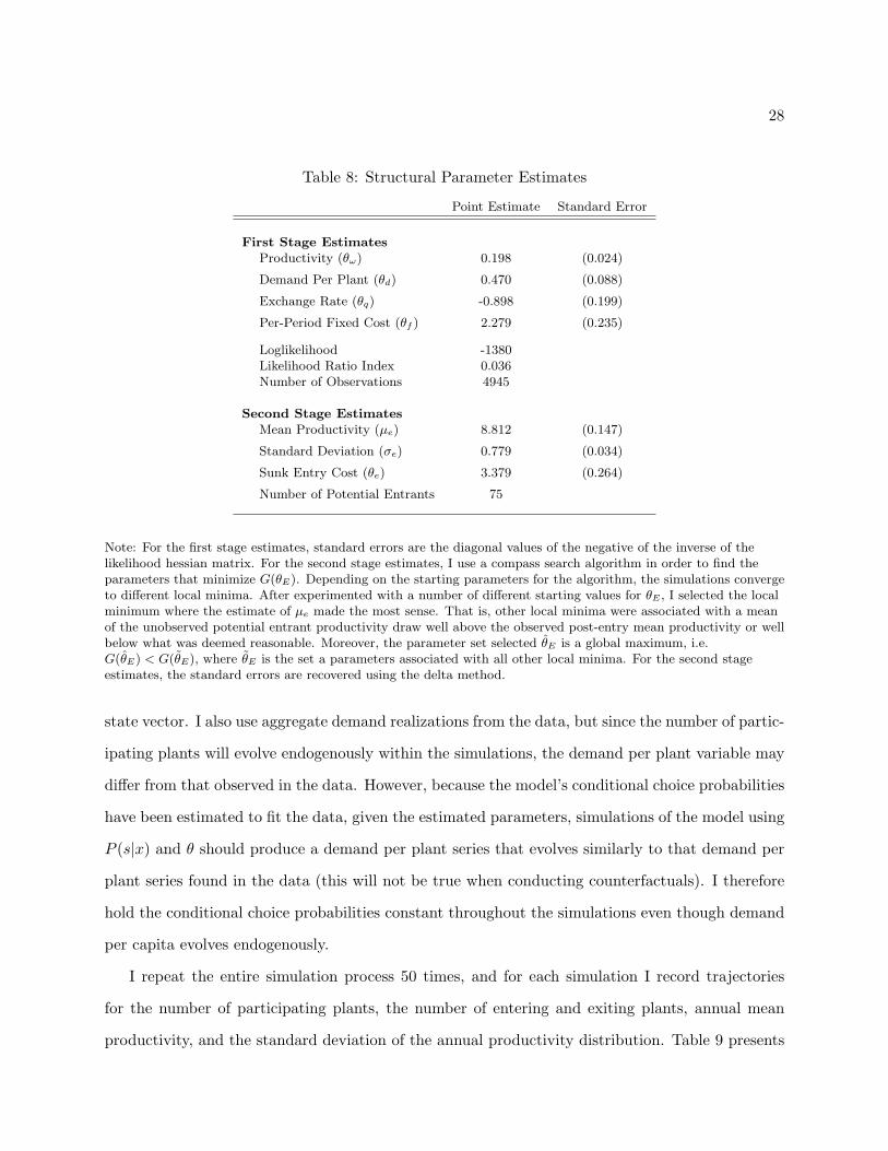
dicount factor to 0.95. Table 8 reports the parameter estimates of the structural model. We would

expect to find that {θω, θd, θf , θe} > 0 and θq < 0, and this is indeed the case. Focusing first on the

variable profit parameters, we see that the parameter on the real exchange rate variable is both

negative and significant, meaning that the real exchange rate, and plants’ perceptions over future

values of the real exchange rate, have an impact on a plant’s chances of survival. Put another way,

depreciations (appreciations) of the real exchange rate increase (decrease) the probability that a

given plant will stay in the market. This is consistent with my hypothesis and the findings in Baggs,

Beaulieu and Fung (2009). The positive and significant parameter on productivity indicates that

plants with lower measured productivity are more likely to exit the market than more productive27I have estimated the model using LP and ACF generated productivity and the results are similar. The first-stage

parameter estimates using LP, ACF and OLS generated productivity are available upon request.

27

producers, which again is consistent with my hypothesis and with many other micro-level studies.

Finally, the positive and significant parameter on the competition variable—or demand per plant—

indicates that either higher aggregate demand or fewer competing plants (or both) increases the

chance of plant survival. All of this implies that less productive plants are more likely to exit the

market when there is an appreciation of the real exchange rate, and more likely to stay in the

market when there is a depreciation.

As for the entry parameters, we see that the estimated mean of the unobserved potential entrant

productivity draw (8.812) is below the observed post-entry mean productivity (9.128), implying that

more productive potential entrants are self-selecting into the market. I also find that entry costs

are approximately 48 percent larger than the per-period fixed cost. While this may seem like a

small entry cost relative to the per-period fixed cost, it is important to note that in assuming that

the payoff to an exiting plant is zero in the first estimation stage, I am implicitly normalizing the

exit value to zero. The result of this normalization is that the per-period fixed cost estimate will

include a part of the exit payoff—that is, the true per-period fixed cost will be lower than the θf

parameter estimate. However, it is not possible to distinguish between the per-period fixed cost

and the exit payoff, making it difficult to draw conclusions by comparing the estimated values of

θe and θf . The estimated standard deviation of the productivity draw (0.779) is lower than the

standard deviation of the post-entry productivity (0.828).

To assess the fit of the model, I begin with the original 135 incumbent plants in operation

in 1973—identified only by their productivity levels—and add the pool of potential entrants pe,

who each receive a productivity draw from the distribution Γe. Each of these 135 + pe plants

then observes their current period private information, and together with last period’s observable

state decide whether to participate in the market or not. Those that do participate become the

next period’s incumbent plants and their productivity levels evolve according to (11). At this

point, another pe potential entrants are added to this new group of incumbents, and the process

is repeated. The model then evolves with random draws on the private information variable ε, the

productivity process’s stochastic term υω, and draws from Γe. I simulate the model forward 25

periods to match the sample time span.

Period by period I substitute actual exchange rate realizations from the data into each plant’s

28

Table 8: Structural Parameter Estimates

Point Estimate Standard Error

First Stage EstimatesProductivity (θω) 0.198 (0.024)

Demand Per Plant (θd) 0.470 (0.088)

Exchange Rate (θq) -0.898 (0.199)

Per-Period Fixed Cost (θf ) 2.279 (0.235)

Loglikelihood -1380Likelihood Ratio Index 0.036Number of Observations 4945

Second Stage EstimatesMean Productivity (µe) 8.812 (0.147)

Standard Deviation (σe) 0.779 (0.034)

Sunk Entry Cost (θe) 3.379 (0.264)

Number of Potential Entrants 75

Note: For the first stage estimates, standard errors are the diagonal values of the negative of the inverse of thelikelihood hessian matrix. For the second stage estimates, I use a compass search algorithm in order to find theparameters that minimize G(θE). Depending on the starting parameters for the algorithm, the simulations convergeto different local minima. After experimented with a number of different starting values for θE , I selected the localminimum where the estimate of µe made the most sense. That is, other local minima were associated with a meanof the unobserved potential entrant productivity draw well above the observed post-entry mean productivity or wellbelow what was deemed reasonable. Moreover, the parameter set selected θE is a global maximum, i.e.G(θE) < G(θE), where θE is the set a parameters associated with all other local minima. For the second stageestimates, the standard errors are recovered using the delta method.

state vector. I also use aggregate demand realizations from the data, but since the number of partic-

ipating plants will evolve endogenously within the simulations, the demand per plant variable may

differ from that observed in the data. However, because the model’s conditional choice probabilities

have been estimated to fit the data, given the estimated parameters, simulations of the model using

P (s|x) and θ should produce a demand per plant series that evolves similarly to that demand per

plant series found in the data (this will not be true when conducting counterfactuals). I therefore

hold the conditional choice probabilities constant throughout the simulations even though demand

per capita evolves endogenously.

I repeat the entire simulation process 50 times, and for each simulation I record trajectories

for the number of participating plants, the number of entering and exiting plants, annual mean

productivity, and the standard deviation of the annual productivity distribution. Table 9 presents

29

cross-simulation averages compared against the observed data moments, and to summarize the

degree of variation across simulations, I report the 10th and 90th percentile simulations. Overall,

the simulations do a very good job of replicating the data, as almost all actual values fall within

the 10th and 90th percentile bounds (the actual mean number of plants lies just outside the 90th

percentile bound).

Table 9: Model Fit

Data Moments Simulation Moments (10th, 90th)

Mean Number of Plants 200.4 197.5 (193.6, 200.0)

Mean Entry Rate (%) 10.40 10.06 (9.64, 10.42)

Mean Exit Rate (%) 8.10 8.11 (7.70, 8.49)

Mean Productivity Level 9.37 9.37 (9.33, 9.39)

Std Productivity Level 0.87 0.88 (0.87, 0.90)

Note: The results based on 50 simulations, using LP2 productivity.

6 Simulated Response to Exchange Rate Shocks

The advantage of estimating a structural model is that it can be used to test counterfactuals,

which shed light on important policy issues. In this section, I examine the model’s response—and

in particular the response of average productivity—to permanent and transitory shocks to the real

exchange rate process. I begin by examining the effect of a one-time negative 20 percent shock to

the real exchange rate process. Because the exchange rate follows a random walk process, the one-

time negative shock will have a permanent effect on the value of the exchange rate. Following this, I

analyze the effect of a one-time negative 20 percent shock to the exchange rate process, followed by

a series of smaller positive shocks that offset the original negative shock after four periods. In this

second counterfactual experiment, the initial shock will be temporary, or transitory, as opposed to

being permanent. These experiments will highlight important features of the model, and provide a

better understanding of the dynamic relationship between the real exchange rate, plant entry and

exit, and industry productivity.28

28In earlier versions of this paper I examined a number of different counterfactual experiments. It was determinedthat the comparison of a permanent shock and offsetting transitory shocks to the exchange rate process was the mostenlightening experiment for understanding the effects of movements in the exchange rate on productivity.

30

I begin by simulating the exchange rate for the benchmark model and the two counterfactual

experiments. For the benchmark simulation, I start with the exchange rate at 0.9 (that is, the

Canadian dollar is worth 0.9 U.S. dollars) and use the relevant VAR parameters from (12) to sim-

ulate the exchange rate out 25 periods, and I do this 1000 times. Averaging over these simulations

gives me a single (benchmark) exchange rate series. For the counterfactual experiments, I shock

the benchmark exchange rate process, and Figure 4 shows the path of the exchange rate for each

counterfactual as the percentage change from the benchmark exchange rate. I treat these three

exchange rate series as exogenous variables when simulating the model.

(a) Permanent Shock (b) Transitory Shock

Figure 4: Percentage Change in the Exchange Rate from Benchmark Model

The model simulations proceed much as they did to test the fit of the model (outlined in

the previous section), except that plant beliefs—modeled as the state-to-state transition matrix

f(x′|x)—and hence the conditional choice probabilities, must adjust to take account of the new

exchange rate processes and the resulting effect on aggregate demand per plant (an endogenous

variable).29 That is, altering the real exchange rate process is likely to affect the number of

plants that participate in the market, which means that the initial beliefs over the evolution of

the demand per plant variable may no longer be consistent with the outcome of the simulations.

In order to account for this, I update plant beliefs about the evolution of demand per plant—and29While the number of plants is an endogenous variable and evolves within the simulations, total demand is

exogenous and must be simulated on its own, like the exchange rate. In order to do this, I regress total demand onthe lagged values of aggregate demand and the exchange rate, and use the resulting parameters to get a simulatedseries for total demand, following the same methodology used to get the simulated exchange rate series.

31

hence the state transition matrix and plant conditional choice probabilities—within each simulation

until plant beliefs are consistent with the simulation outcome. Appendix D provides the detailed

algorithm used to run the simulations. In brief, the simulation outcomes represent a fixed point

in both conditional choice probabilities and beliefs about the evolution of demand per plant.30 In

each case, plant beliefs about the exchange rate process remain unchanged. I simulate the model

500 times, and then average across simulations.

Figure 5 shows the reaction of mean productivity in each of the two experiments (presented

as percentage change from benchmark model). In the case of a permanent shock, Figure 5(a), we

see a drop of almost 4.5 percent in mean productivity upon impact, but the effect of the shock

deteriorates over time as productivity returns to the level of productivity in the benchmark model

– even though the exchange rate remains low. After 25 periods, mean productivity ends up being

about 1 percent below mean productivity in the benchmark model. For the transitory shock, Figure

5(b), aggregate productivity drops by more than 2 percent upon impact and then returns quickly to

the level of the benchmark model. In fact, there is an overshoot, as mean productivity goes to 0.5

percent above mean productivity in the benchmark model before heading back towards benchmark

productivity and then ending up a little over 0.5 percent above the benchmark model.

(a) Permanent Shock (b) Transitory Shock

Figure 5: Percentage Change in Mean Productivity from Benchmark Model

From the setup of the model, it is clear that the initial drop in productivity in both the per-30This process is similar to the computational algorithm developed in Krusell and Smith (1998). They use an

iterative process to approximate an equilibrium by updating firm beliefs about the evolution of an endogenousvariable of interest.

32

manent and transitory shock counterfactuals is driven by the fact that less productive plants are

staying in the market—when they are otherwise forced out in the benchmark model—and possibly

crowding out new more productive entrants. For the transitory shock, we would expect to see

average productivity return to the level of productivity in the benchmark model after the initial

shock is mitigated, which it does. However, the fact that mean productivity in the permanent shock

counterfactual also returns to the level of productivity in the benchmark model deserves further

study.

For a deeper understanding of what is driving these changes in mean productivity, Figure 6

reports the mean productivity of exiting plants.31 For the permanent shock, presented in Figure

6(a), there is an immediate drop of about 13 percent in the mean productivity of exiting plants,32

reflecting that fact that less productive plants are able to stay in the market. Interestingly, mean

exiting plant productivity remains below the benchmark model, even though overall mean produc-

tivity returns to the level of productivity in the benchmark model. Because entry and exit are only

the only factors affecting aggregate productivity in this model, it must be that the average entrant

is becoming more productive over time, which drives up overall mean productivity. The intuition

for this is clear. Upon impact, the negative shock to the exchange rate allows less productive plants

to stay in the market when they otherwise would have been forced out, and allows an initial surge

in the number of entrants. This not only drives down exit plant mean productivity, but mean

entering plant productivity, as well, leading to a decrease in overall mean productivity. However,

as the number of participating plants increases, new plants must be more productive to overcome

the cost of entry, which drives up mean productivity of entering plants, leading to an increase in

overall mean productivity.

In the case of the transitory shock, presented in Figure 6(b), we see an immediate drop in mean

productivity of exiting plants of 2.7 percent, but that productivity quickly returns to the level of the

benchmark model, and then drops again to about 3.5 percent below the benchmark model. This31Presenting the results for the mean productivity of entrants could be enlightening. However, in the benchmark

model, the exchange rate remains relatively high and therefore there is very little entry. The result is that a comparisonof the counterfactual results against the benchmark model is not particularly informative.

32For both the permanent and transitory exchange rate shock counterfactuals, there are no exiting plants in thefirst period, which explains why Figures 6(a) and 6(b) show no deviation from the benchmark model in the firstperiod following the shock.

33

(a) Permanent Shock (b) Transitory Shock

Figure 6: Percentage Change in Mean Productivity of Exiting Plants from Benchmark Model

reflects the fact that low productivity plants stay in the market following the initial drop in the

exchange rate, but then are forced from the market as the exchange rate returns to the pre-shock

level.

Finally, Figure 7 reports the change in the number of participating plants in each case. As

expected, a permanent decrease in the real exchange rate leads to significantly more participating

plants, while a transitory shock results in an initial increase in the number of participating plants,

but the relative number of plants decreases as the exchange rate returns to its pre-shock level.

(a) Permanent Shock (b) Transitory Shock

Figure 7: Percentage Change in the Number of Plants from Benchmark Model

Overall, these results point to the fact that movements the real exchange rate can lead to

turnover-induced productivity changes. However, the interesting result is that in each case, mean

34

productivity returns to, or exceeds, the level of productivity in the benchmark model, even if the

exchange rate remains permanently below that level, suggesting that movement in—rather then

the level of—the exchange rate can lead to turnover-induced productivity changes.

7 Conclusions

This paper offers a distinct approach to studying one channel through which movements in the real

exchange rate can affect aggregate productivity. By modeling the decisions of individual plants, I am

able to capture how movements in the real exchange rate affect the makeup of plants that populate

the market for agricultural implements. Moreover, in allowing for heterogeneous potential entrants,

the model incorporates a self-selection mechanism, whereby more productive potential entrants self-

select into the market. This is made possible by a two-stage estimation procedure, where the mean

and standard deviation of the unobserved potential entrant productivity distribution, along with

the cost of entry, are estimated in the second stage.

The structural parameter estimates confirm that a depreciation (appreciation) of the real ex-

change rate increases (decreases) the probability that a given plant will stay in the market, and that

higher productivity plants are more likely to stay in the market. Using the structural parameter

estimates, I conduct a series of counterfactual exercises that examine the effect of different types

of real exchange rate depreciations. Results show that while large exchange rate shocks can have

an immediate impact on aggregate productivity through plant turnover, there is little effect in the

long run.

Although this study focuses on a single industry within the Canadian manufacturing sector, it

provides insight into the consequences of exchange rate movements, which is an important policy

issue for many countries, not just Canada.

35

Appendices

A Hybrid Levinsohn-Petrin

LP2 Method:

• Run a regression of rit on mit to obtain an estimate of the function E(rit|mit).

• Run the regressions of lit, eit and yIt on mit to get E(lit|mit), E(eit|mit) and E(yIt|mit).

• Let Y (mit) = rit − E(rit|mit), X1(mit) = lit − E(lit|mit) , X2(mit) = eit − E(eit|mit) andX3(mit) = yIt − E(yIt|mit).

• Regress Y on the constructed independent variables (X1, X2, X3) to obtain estimates of βl,βe, and βη.

B AR(1) and VAR Coefficient Estimates

Parameter Estimate s.e.

(1− ρω)ω 2.346* 0.100ρω 0.759* 0.010ρdd 0.857* 0.059ρdq 0.458* 0.157

∗ Indicates estimate is significant at the 1% level.

C NPL Algorithm

The Nested Pseudo-Likelihood algorithm can be laid out in four steps:

1. Begin by guessing values for the conditional choice probabilities plants are using via a con-sistent estimate of the conditional choices P k(sj |x), where the index denoted by k is initially0 (referring to the policy iteration). I estimate P 0 using a simple non-parametric frequencyestimator.

2. Given parameter estimate θkI , and the guess at player’s conditional choices P k, use the policy

operator Ψ(sj |x, P k, θkI ) to estimate the model via maximum likelihood:

θk+1I = arg max

θI

L∑l=1

lnΨ(sl|xl, Pk, θk

I ) (21)

where sl is the action taken by a firm in state xl, and l indexes observations.

36

3. Update the guess at the equilibrium strategy as:

P k+1(sj |x) = Ψ(sj |x, P k, θk+1I ) (22)

for all actions sj ∈ S and observable states x ∈ X.

4. Repeat steps 2-3 until the difference between the k and k+1 stage estimates of the conditionalchoice probabilities is below some minimum tolerance parameter.

With the assumption that the per-period profit function is separable in the dynamic parameters,i.e. π(x, s|θ) = h(x, s) · θ, I can follow closely the methodology in AM, and define H(s) as thematrix with rows h(x, s) for each value of x. With this, the policy operator (17) can be expressedas:

Ψ(sj |x, P, θ) =exp

{h(x, sj)θ + e(x, sj)

}∑

k exp{

h(x, sk)θ + e(x, sk)}

where h(x, s) is a row the the matrix:

f(s)H(s) + βf(s)[IM − βf(P )

]−1 ∑j∈J

P (j) ∗H(j)

and e(x, s) is an element in the vector:

βf(s)[IM − βf(P )

]−1 ∑j∈J

P (j) ∗[γ − lnP (j)

]where f(P ) =

∑j∈J P (j) ∗ f(s).

37

D Counterfactual Algorithm

1: Obtain simulated real exchange (q) and demand per plant (d) series using VAR parameters2: repeat3: Update transition matrix f(x′|x)4: Obtain estimate of P k (initially k = 0)5: repeat6: V = V I(x|s, P k, θI)7: P k+1 = exp(V )

1+exp(V )

8: ∆1 = max(|P k+1 − P k|)9: P k = P k+1

10: until ∆1 ≤ γ1

11: Simulate model S times and obtain the new series for demand per plant d′

12: ∆2 = max(|d′ − d|)13: d = d′+d

214: d = d15: Re-estimate VAR parameters given d16: until ∆2 ≤ γ2

17: Simulate model T times and average over simulations (note: in order to speed up thecounterfactual process, it may be the case that T > S)

References

Ackerberg, D., K. Caves and G. Frazer (2006): “Structural Identification of Production Functions,”Working Paper (December 2006).

Aguirregabiria, V. and P. Mira (2002): “Swapping the Nested Fixed Point Algorithm: A Class ofEstimators for Discrete Markov Decision Models,” Econometrica 70(4), pp. 1519-1543.

——– (2007): “Sequential Estimation of Dynamic Discrete Games,” Econometrica 75(1), pp. 1-53.

Baggs, J., E. Beaulieu and L. Fung (2009): “Firm Survival, Performance, and the Exchange Rate,”Canadian Journal of Economics 42(2), pp. 393-421.

Bajari, P., L. Benkard and J. Levin (2007): “Estimating Dynamic Models of Imperfect Competi-tion,” Econometrica 75(5), pp. 1331-1370.

Baldwin, J. and W. Gu (2003): “Plant Turnover and Productivity Growth in Canadian Manufac-turing,” Economic Analysis (EA) Research Paper Series, Statistics Canada, Catalogue No.11F0019 No. 193 (April 2003).

——– (2006): “Competition, Firm Turnover and Productivity Growth,” Economic Analysis (EA)Research Paper Series, Statistics Canada, Catalogue No. 11F0027MIE No. 42 (September2006).

38

——– (2007): “Log-term Productivity Growth in Manufacturing in Canada and the United States,1961 to 2003,” The Canadian Productivity Review Catalogue No. 15-206-X (December 2007).

Bernard, A., J. Eaton, J. Jensen and S. Kortum (2003): “Plants and Productivity in InternationalTrade,” American Economic Review 93(4), pp. 1268-1290.

Bernstein, J, R. Harris and A. Sharpe (2002): “The Widening Canada-US Manufacturing Produc-tivity Gap,” International Productivity Monitor 5, Centre for the Study of Living Standards(Fall 2002).

Bresnahan, T. F. and P. C. Reiss (1991): “Entry and Competition in Concentrated Markets,”Journal of Political Economy 99(5), pp. 977-1009.

Burnside, C., M. Eichenbaum and S. Rebelo (1995): “Capital Utilization and Returns to Scale,”NBER Macroeconomics Annual 10, B. Bernanke and J. Rotemberg eds., pp. 67-110 .

Collard-Wexler, A. (2008): “Demand Fluctuations in the Ready-Mix Concrete Industry,” NYUStern Working Paper (November 2008).

——– (2009): “Productivity Dispersion and Plant Selection in the Ready-Mix Concrete Indsutry,”NYU Stern Working Paper (March 2009).

Das, S., M. Roberts and R. Tybout (2007): “Market Entry Costs, Producer Heterogeneity, andExport Dynamics,” Econometrica 75(3) pp. 837-873.

De Loecker, J. (2007): “Product Differentiation, Multi-Product Firms and Estimating the Impactof Trade Liberalization on Productivity,” NBER Working Paper 13155 (June 2007).

Ericson, R. and A. Pakes (1995): “Markov-Perfect Industry Dynamics: A Framework for EmpiricalWork,” Review of Economic Studies 62(1), pp. 53-82.

Feenstra, R. (1989): “Symmetric Pass-Through of Tariffs and Exchange Rates under ImperfectCompetition: An Empirical Test.” Journal of International Economics 27 (1/2), pp. 25-45.

Ghironi, F. and M. Melitz (2005): “International Trade and Macroeconomic Dynamics with Het-erogeneous Firms,” Quarterly Journal of Economics 120(3), pp. 865-915.

Griliches, Z. and J. Klette (1996): “The Inconsistency of Common Scale Estimators When OutputPrices are Unobserved and Endogenous,” Journal of Applied Econometrics 11(4), pp. 343-361.

Harris, R. G. (2001): “Is There a Case for Exchange-Rate-Induced Productivity Changes?” in L.Schembri (ed.) Re-Visiting the Case for Flexible Exchange Rates, Bank of Canada, Ottawa.

Hopenhayn, H. (1992): “Entry, Exit and Firm Dynamics in Long Run Equilibrium,” Econometrica60(5), pp. 1127-1150.

Hotz, V. and R. Miller (1993): “Conditional Choice Probabilities and the Estimation of DynamicModels,” Review of Economic Studies 60(3), pp. 497-529.

Jovanovic, B. (1982): “Selection and the Evolution of Industry,” Econometrica 50(3), pp. 649-670.

39

Krusell, P. and A. Smith (1998): “Income and Wealth Heterogeneity in the Macroeconomy,”Journal of Political Economy 106(5), pp. 867-896.

Levinsohn, J. and M. Meltiz (2003): “Productivity in a Differentiated Products Market Equilib-rium,” Harvard University, Working Paper.

Levinsohn, J. and A. Petrin (2003): “Estimating Production Functions Using Inputs to Controlfor Unobservables,” Review of Economic Studies 70(2), pp. 317-341.

McFadden, D. (1989): “A Method of Simulated Moments for Estimation of Discrete ResponseModels Without Numerical Integration,” Econometrica 57(5), pp. 995-1026.

Melitz, M. (2003): “The Impact of Trade on Intra-Industry Reallocations and Aggregate IndustryProductivity,” Econometrica 71(6), pp. 1695-1725.

Melitz, M. and G. Ottaviano (2008): “Market Size, Trade, and Productivity,” Review of EconomicStudies 75, pp. 295-316.

Olley, S. and A. Pakes (1996): “The Dynamics of Productivity in the Telecommunications Equip-ment Industry,” Econometrica 64(6), pp. 1263-1297.

Pakes, A., M. Ostrovsky and S. Berry (2004): “Simple Estimators for the Parameters of DiscreteDynamic Games,” NBER Working Paper 10506.

Pakes, A. and D. Pollard (1989): “The Asymptotic Distribution of Simulation Experiments,”Econometrica 57(5), pp. 1027-1057.

Pavcnik, N. (2002): “Trade Liberalization, Exit, and Productivity Improvements: Evidence fromChilean Plants,” Review of Economic Studies 69(1), pp. 246-276.

Rust, J. (1987): “Optimal Replacement of GMC Bus Engines: An Empirical Model of HaroldZurcher,” Econometrica 55(5), pp. 999-1033.

Tauchen, G. (1986): “Finite State Markov-Chain Approximations to Univariate and Vector Au-toregressions,” Economics Letters 20, pp. 171-181.

Tomlin, B. and L. Fung (2009): “The Effect of Real Exchange Rate Movements on HeterogeneousPlants: A Quantile Regression Analysis,” Working Paper (April 2009).

Trefler, D. (2004): “The long and Short of the Canada-U.S. Free Trade Agreement,” AmericanEconomic Review 94(4), pp. 870-895.

Weintraub, G., L. Benkard and B. Van Roy (2007): “Markov Perfect Industry Dynamics withMany Firms,” Econometrica 76(6), pp.1375-1411.

Xu, Y. (2008): “A Structural Empirical Model of R&D, Firm Heterogeneity and Industry Evolu-tion,” NYU Working Paper (November 2008).