exact artificial boundary conditions for continuum and discrete...

SIAM J. APPL. MATH. c© 2006 Society for Industrial and Applied MathematicsVol. 66, No. 5, pp. 1749–1775

EXACT ARTIFICIAL BOUNDARY CONDITIONS FORCONTINUUM AND DISCRETE ELASTICITY∗

SUNMI LEE† , RUSSEL E. CAFLISCH‡ , AND YOUNG-JU LEE†

Abstract. For the continuum and discrete elastic equations, we derive exact artificial boundaryconditions (ABCs), often referred to as transparent boundary conditions, that can be applied at aplanar interface below which there are no forces. Solution of the elasticity equations can then beperformed using this interface as an artificial boundary, often with greatly reduced computationaleffort, but without loss of accuracy. A general solvability requirement is presented for the existenceof an artificial boundary operator for discrete systems (such as discrete elasticity) on an unbounded(semi-infinite) domain. The solvability requirement is validated by introducing a sum-of-exponentialsansatz for the solution below the artificial boundary. We also derive a new expression for the totalenergy for the system, involving only the region above the artificial boundary. Numerical examplesare provided to confirm and illustrate the accuracy and effectiveness of the results.

Key words. elasticity, discrete elasticity, artificial boundary conditions, transparent boundaryconditions, atomistic strain

AMS subject classifications. Primary, 65N55; Secondary, 74B05, 70C20

DOI. 10.1137/050644252

1. Introduction. Many of the boundary value problems arising in applied math-ematics are formulated on unbounded domains. It is in general a nontrivial task tosolve such problems numerically [6], since the numerical solution naturally requiresboundary conditions at a finite depth in the body.

The main motivation of the present work comes from the numerical simulation ofstrain fields in semi-infinite domains. For the strain equations, the use of a physicalboundary condition, such as the zero displacement field at a certain depth, has beena common practice [21]. On the other hand, due to the long range of elastic interac-tions, the zero boundary condition must be imposed at considerable depth in orderto accurately compute the strain field [4], which entails large computational cost.

The purpose of this paper is to derive exact artificial boundary conditions (ABCs)such that the solution on the (bounded) computational domain coincides with theexact solution on the unbounded domain. Such exact artificial boundary conditionsare oftentimes referred to as transparent boundary conditions (TBCs) [6].

There have been various works on ABCs for a wide range of problems. For exam-ple, certain ABCs for the Poisson and Helmholtz equations on infinite domains areinvestigated in [1] using domain decomposition and Fourier techniques. For generalelliptic problems, approximate ABCs and error estimates are performed within thefinite element framework in [3]. Boundary element methods for homogeneous elasto-

∗Received by the editors November 4, 2005; accepted for publication (in revised form) April 20,2006; published electronically July 31, 2006. This research was supported in part by the MARCOCenter on Functional Engineered NanoArchitectonics (FENA) and by the NSF through grant DMS-0402276.

http://www.siam.org/journals/siap/66-5/64425.html†Department of Mathematics, University of California at Los Angeles, 520 Portola Plaza, Los An-

geles, CA 90095 ([email protected], [email protected], http://www.math.ucla.edu/∼yjlee).The first author was partially supported by the National Institute for Mathematical Sciences, Korea.

‡Department of Mathematics and Department of Materials Science and Engineering, Universityof California at Los Angeles, 520 Portola Plaza, Los Angeles, CA 90095 ([email protected],http://www.math.ucla.edu/∼caflisch).

1749

1750 SUNMI LEE, RUSSEL E. CAFLISCH, AND YOUNG-JU LEE

static and elastodynamic cases, linear elastostatic problems, time dependent heat andwave equations, and electromagnetic scattering problems are also treated in an exactmanner using the Dirichlet to Neumann boundary condition in [2, 7, 8, 9].

For the elasticity problem, several local and nonlocal artificial boundary condi-tions are provided in terms of the finite element formulation in [12, 13, 14]. For adiscrete elastic strain model for an epitaxial thin film, ABCs were derived recentlyby Russo and Smereka [20] using a formulation that is somewhat different from ourmodel.

In the present work, we perform an analysis for the equations of both continuumand discrete elastic models. The discrete elastic equations correspond to an atomisticstrain model introduced in the recent work by Schindler et al. [21]. Although fulldetails are provided only for a discrete strain model, a general solvability requirementis formulated, which results in the well-posedness or the solvability of the system inan infinite domain. This work is a discrete analogue of the work by Hagstrom andKeller [11]. The solvability requirement is then validated by analyzing the solution onthe exterior domain using a sum-of-exponentials ansatz. This framework, on the onehand, leads us to derive the abstract ABC operator in the form of a Schur complementoperator and, on the other hand, guides the construction of the explicit ABC operatorfor actual implementations. Thanks to the ABC operator, the force balance equationthat needs to be solved in the infinite domain can be posed as a reduced equationon the bounded domain, whose solution has been shown to coincide with the exactsolution on the full (unbounded) domain. In addition, a new formula is derived forthe total elastic energy of the system, involving only the solution above the artificialboundary. The latter is particularly important for practical applications such as thinepitaxial film growth simulations.

The rest of the paper is structured as follows. In section 2, we introduce somepreliminaries and notation to ease the presentation. The ABCs, total energy formula,and variational principle for continuum elasticity are derived in section 3. In section 4,we briefly review the discrete elastic strain model and introduce the general solvabilityrequirement, present an abstract form of the ABC operator, and derive explicit ABCsfor a specific discrete strain model. The total energy formula and the variationalprinciple for the discrete strain model are also presented. Several illustrative numericalresults are provided in section 5. Conclusions are discussed in section 6. Some detailsare saved for the appendix.

2. Preliminaries. Suppose that the domain Ω is a half-infinite body, e.g., Ω ={(x, y, z) ∈ R

3 : z < h(x, y)} for h : R2 �→ R being a bounded function. See Figure 2.1

for a schematic description. The interface Γ2 on which the artificial boundary will beimposed is illustrated in Figure 2.1. For both the continuum and discrete problems,the domain Ω is divided into a finite part Ω1 and a semi-infinite part (an exteriordomain) Ω2 = Ω\Ω1. The requirement on the choice of Ω2 is that its boundary Γ2

is planar and normal to the depth variable and that there are no external forces inΩ2. For the boundary condition for both continuum and discrete elasticity equations,we assume that the periodic conditions are imposed in x- and y-directions (lateraldirections) and that the Neumann condition (i.e., the variational principle with noconstraint at the boundary) is imposed on the top layer Γ1 unless explicitly statedotherwise. Use of the Neumann condition is only for simplicity and to ensure that theproblem is well-posed; it does not influence the resulting ABCs.

We use boldface lower case letters for vectors in Rd with d = 2 or 3 and boldface

capital letters for symmetric tensors or square matrices. The differential operator ∂kdenotes the partial derivative with respect to the kth coordinate variable, i.e., ∂/∂xk,

EXACT ARTIFICIAL BOUNDARY CONDITIONS 1751

ΩΩ

Ω

Γ

Γ

Γ1 1

2

1

2

Fig. 2.1. The domain decomposition: An artificial boundary Γ2 (the horizontal plane) dividesΩ into Ω1 and Ω2. Γ1 is the top boundary (surface) of Ω.

and the operator ∇· is the standard divergence operator defined through

∇· = (∂/∂x, ∂/∂y) · for d = 2,

∇· = (∂/∂x, ∂/∂y, ∂/∂z) · for d = 3.

The notation ∇ denotes the usual gradient operator for d = 2 and d = 3 given,respectively, as

∇ =

(∂/∂x∂/∂y

), ∇ =

⎛⎝ ∂/∂x

∂/∂y∂/∂z

⎞⎠ ,

and Δ is the Laplace operator ∇ · ∇.For two vectors u and v, u · v is the dot product; for a vector v = (vk)k=1,...,d

and a tensor N = (Nkl)k,l=1,...,d, v · N =∑d

k=1 vkNk�. The magnitude of a vector uwill be denoted by |u| = (u · u)1/2.

Although the letters i, j, k are used for indices, we shall also use ı to denote theimaginary unit

√−1, and the complex conjugate of a complex number υ shall be

denoted by υ. Also, for the matrix N, NH and NT denote the complex conjugatetranspose and the real transpose of N, respectively. Finally, we shall use χ to denotethe usual characteristic function that is defined as

χ(x) =

{1 for x ∈ Ω1,0 for x /∈ Ω1.

(2.1)

Some other notation will be introduced in each section as necessary.

3. The ABCs for continuum elasticity. In this section, we review the con-tinuum elastic equations from an energetic viewpoint. We then derive the artificialboundary (or ABC) operator A, as well as a new expression for the total energy anda formulation of the force balance equations depending on only the displacement onand above the interface Γ2 on which the artificial boundary condition is given.

3.1. Continuum elasticity. Continuum elasticity is formulated in terms of adisplacement field u = u(x) = y(x) − x between the equilibrium position x of amaterial point and the elastically deformed position y(x) of that point. The straintensor S has components defined as Sk� = (∂ku� + ∂�uk)/2 in which uk are thecomponents of u.

The derivation of the linear elasticity equations can be made via a variationalprinciple for the total energy E in a domain Ω, namely,

δE = 0.(3.1)


The total elastic energy E for the linear elasticity is given as follows:

E =

∫Ω

Edx,(3.2)

where the integrand is the energy density

E =1

2

∑k,�

Sk�Tk� − u · f χ,(3.3)

f = (fk) is a body force, and T = (Tk�) is the stress tensor defined, for an isotropicmaterial, as

Tk� = λδk�∑i

Sii + 2τSk�.(3.4)

The parameters λ and τ are the Lame constants. In the absence of external force onthe boundary Γ1, (3.1) reduces to the classical Navier equations of linear elasticity,i.e.,

−∇ · T = fχ in Ω,(3.5)

n · T = 0 on Γ1,

where n is the outer unit normal vector.For linear elasticity with cubic symmetry, the elastic energy density E is the

following:

E =C11

2

∑i

S2ii + 2C44

∑k �=�

S2k� + C12

∑k �=�

SkkS��,(3.6)

where C11, C44, and C12 are the cubic elastic moduli, i.e., the Voigt constants. Thelinear elasticity equations with cubic symmetry are

−C11∂k∂kuk − C44

∑l �=k

∂l∂luk(3.7)

− (C12 + C44)∑l �=k

∂k∂lul = fkχ in Ω

for k = 1, . . . , d. Note that the isotropic linear elasticity equations (3.5) can berecovered from (3.7) by choosing the following Voigt constants:

(C11, C44, C12) = (λ + 2τ, τ, λ).(3.8)

For the study of the ABCs for continuum elasticity, we restrict our attention tothe isotropic linear elasticity, namely, (3.7) with the Voigt constants given in (3.8),for simplicity. It is easily generalized to the anisotropic case.

3.2. Two dimensional case. In this section, we construct the artificial bound-ary operator A for the two dimensional case. The main idea is to analytically solvethe force balance equation (3.7) on the exterior domain Ω2 by introducing a sum-of-exponentials ansatz, which must be modified to include algebraic terms.


We assume that the solution is periodic in the x-direction with 2π periodicity andthat the interface Γ2 is a line, i.e., Γ2 = {(x, y) ∈ R

2 : y = 0}. We first look for amodal solution u(x, y) for y < 0 as

u(x, y) = u(μ, y) eıμx(3.9)

= u(μ) eβy eıμx =

(u(μ)v(μ)

)eβy eıμx.

Since u in (3.9) is the solution to (3.7), for each μ, u(μ) should satisfy the followinglinear system:

M(μ, β)u(μ) = 0,

where u(μ) = (u(μ), v(μ))T and

M(μ, β) =

(−(λ + 2τ)μ2 + τβ2 ıμ(λ + τ)β

ıμ(λ + τ)β −τμ2 + (λ + 2τ)β2

).

A nontrivial solution can be attained only if

detM(μ, β) = τ(λ + 2τ)(β2 − μ2)2 = 0,(3.10)

which implies that β = ±|μ|. Since the solution u should decay as y → −∞, thenβ = |μ| is the proper choice. Note that for μ = 0, the only solution is β = 0, whichcorresponds to a trivial solution, the constant displacement field.

We now compute the zero eigenvector for M(μ, |μ|). It is easy to see that thematrix M(μ, |μ|) has a zero eigenvector given by q1 = (ı, μ/|μ|)T and a generalizedeigenvector q2 = (0,−c/μ)T satisfying M(μ)q1 = 0 and M(μ)q2 = −(λ + 3τ)|μ|q1

with c = (λ + 3τ)/(λ + τ), from which we obtain the general solution to the equation(3.7) as follows:

u(μ, y) = ((aμ + bμy)q1 + bμq2) eıμx+|μ|y,(3.11)

where

aμ = −u(μ, 0)ı and bμ = −c−1(μv0(μ, 0) + ı|μ|u(μ, 0)).(3.12)

From this, we obtain the following simple but important lemma.Lemma 3.1. A solution to (3.7) on the domain Ω2 with a given boundary value

u0(x) on Γ2 is given by the following:

u(x, y) =1

2π

∫ 2π

0

G(x− x′, y)u0(x′)dx′,(3.13)

where G is defined, using c = (λ + 3τ)/(λ + τ), as

G(x− x′, y) =

∞∑μ=−∞

Gμ(x− x′, y),

Gμ(x− x′, y) =

⎛⎝ 1 + |μ|

c y −μc ıy

−μc ıy 1 − |μ|

c y

⎞⎠ e|μ|y eıμ(x−x′).

This analytic expression for the solution u on the domain Ω2 is used to derive theABC operator.


3.3. The ABC operator for the two dimensional case. In this section,using Lemma 3.1, we construct the ABC operator. First, consider the expression ofthe solution u in the exterior domain Ω2 given in (3.13). By taking the derivative ofu with respect to y, one finds that

∂y(u(x, y)) =1

2π

∫ 2π

0

∂y(Gμ(x− x′, y))u0(x′) dx′.(3.14)

Note that the normal component of the stress tensor n · T is given by

n · T =

(τ(∂yu + ∂xv)

(λ + 2τ)∂yv + λ∂xu

),(3.15)

and observe that it can be written in terms of u on the interface Γ2 as follows:

n · T =

∞∑μ=−∞

1

2π

∫ 2π

0

Aμu0(x′) dx′,(3.16)

where

Aμ =2

λ + 3τ

(τ(λ + 2τ)|μ| τ2ıμ

−τ2ıμ τ(λ + 2τ)|μ|

)eıμ(x−x′).(3.17)

Define the artificial boundary operator A by the following:

Au0(x) =

∞∑μ=−∞

1

2π

∫ 2π

0

Aμu0(x′) dx′.(3.18)

It is interesting to note that the operator A is real and symmetric since Aμ(x−x′) =AH

μ (x′ − x).

3.4. The ABC operator for the three dimensional case. We now extendthe previous analysis to the three dimensional case by constructing the solution of thehomogeneous linear elasticity problem in a semi-infinite domain, Ω2. Assume thatΓ2 is the plane z = 0. As in the two dimensional case, assume that in the lateraldirection, the solution is periodic with 2π periodicity for both variables, x and y. Thefollowing result is the analogue to Lemma 3.1.

Lemma 3.2. A solution to (3.7) with given boundary data u0(x, y) on the interfaceΓ2 is given by the following:

u(x, y, z) =1

4π2

∫ 2π

0

∫ 2π

0

G(x− x′, y − y′, z)u0(x′, y′) dx′dy′,(3.19)

where G is defined, using c = (λ + 3τ)/(λ + τ) and d = |(μ, ν)|, as

G(x− x′, y − y′, z)

=∞∑

μ,ν=−∞

⎛⎜⎜⎜⎝

1 + μ2

cdz μν

cdz −μ

cız

μνcd

z 1 + ν2

cdz − ν

cız

−μcız − ν

cız 1 − d

cz

⎞⎟⎟⎟⎠edzeı(μ,ν)·(x−x′,y−y′).


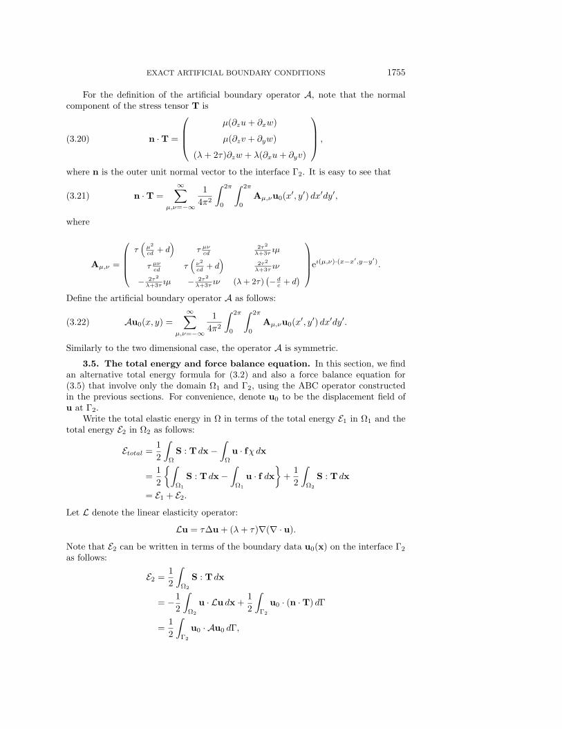
For the definition of the artificial boundary operator A, note that the normalcomponent of the stress tensor T is

n · T =

⎛⎜⎜⎝

μ(∂zu + ∂xw)

μ(∂zv + ∂yw)

(λ + 2τ)∂zw + λ(∂xu + ∂yv)

⎞⎟⎟⎠ ,(3.20)

where n is the outer unit normal vector to the interface Γ2. It is easy to see that

n · T =

∞∑μ,ν=−∞

1

4π2

∫ 2π

0

∫ 2π

0

Aμ,νu0(x′, y′) dx′dy′,(3.21)

where

Aμ,ν =

⎛⎜⎜⎜⎝

τ(

μ2

cd+ d

)τ μν

cd2τ2

λ+3τıμ

τ μνcd

τ(

ν2

cd+ d

)2τ2

λ+3τıν

− 2τ2

λ+3τıμ − 2τ2

λ+3τıν (λ + 2τ)

(− d

c+ d

)

⎞⎟⎟⎟⎠eı(μ,ν)·(x−x′,y−y′).

Define the artificial boundary operator A as follows:

Au0(x, y) =

∞∑μ,ν=−∞

1

4π2

∫ 2π

0

∫ 2π

0

Aμ,νu0(x′, y′) dx′dy′.(3.22)

Similarly to the two dimensional case, the operator A is symmetric.

3.5. The total energy and force balance equation. In this section, we findan alternative total energy formula for (3.2) and also a force balance equation for(3.5) that involve only the domain Ω1 and Γ2, using the ABC operator constructedin the previous sections. For convenience, denote u0 to be the displacement field ofu at Γ2.

Write the total elastic energy in Ω in terms of the total energy E1 in Ω1 and thetotal energy E2 in Ω2 as follows:

Etotal =1

2

∫Ω

S : T dx −∫

Ω

u · fχdx

=1

2

{∫Ω1

S : T dx −∫

Ω1

u · f dx}

+1

2

∫Ω2

S : T dx

= E1 + E2.

Let L denote the linear elasticity operator:

Lu = τΔu + (λ + τ)∇(∇ · u).

Note that E2 can be written in terms of the boundary data u0(x) on the interface Γ2

as follows:

E2 =1

2

∫Ω2

S : T dx

= −1

2

∫Ω2

u · Lu dx +1

2

∫Γ2

u0 · (n · T) dΓ

=1

2

∫Γ2

u0 · Au0 dΓ,


where we use the fact that Lu = 0 in the domain Ω2 and the definition (3.22) of theartificial boundary operator A.

Consequently, the total energy Etotal in the domain Ω is

Etotal = E1 + E2(3.23)

=1

2

∫Ω1

S : T dx −∫

Ω1

u · f +1

2

∫Γ2

u0 · Au0 dΓ.

This is the new formula for the total energy (3.2) that involves only the domain Ω1

and Γ2. Now apply integration by parts to the first term in (3.23) and obtain

Etotal = −1

2

∫Ω1

u · Lu dx −∫

Ω1

u · f dx(3.24)

+1

2

∫Γ2

u0 · Au0 − u0 · (n · T) dΓ.

Application of the variational principle for the new expression of the total energy(3.24) results in the following force balance equations, which use the ABC operatorA in the ABC on Γ2:

−Lu = f in Ω1,

n · T = Au0 on Γ2.

4. The ABCs for discrete elasticity. In this section, we study the analogueof the ABCs for discrete elasticity. In particular, we discuss the solvability (well-posedness) of the discrete strain model in an unbounded or semi-infinite domain.

It is not trivial to show directly the well-posedness of the discrete strain model inan infinite domain. As discussed in Hagstrom and Keller [11], the well-posedness canbe derived from a so-called solvability requirement, which is a solvability condition forthe exterior domain problem for which the force term is zero. Generally, the validationof this solvability requirement is done by introducing a sum-of-exponentials ansatzfor the solution below the artificial boundary. It is difficult, however, to validate thiscondition fully in an analytic manner [11] except for simple problems such as theLaplace equation. Numerical validation is partially used, since an analytic validationcould not be made fully for the current problem of interest.

The importance of the framework developed in this section is that it identifieshow the solvability requirement can be used to show well-posedness of the discreteequations posed on the unbounded domain, and also clarifies why an appropriateuse of the ABC operator leads to the exact boundary condition. To the best of ourknowledge, it is the first attempt to formulate a general discussion on the solvabilityof discrete systems in an infinite domain in terms of solvability requirements. Fur-thermore, this formal discussion leads to an understanding of the ABC operator asa Schur complement operator and reveals various properties of the resulting reducedsystem on the finite domain. These properties of the reduced system are importantwhen one attempts to develop an appropriate solver for the reduced system (see theconcluding remark in section 6).

Throughout this section, we assume that the lattice of the discrete strain modelis connected [19]. We begin this section by briefly reviewing the discrete elastic modelintroduced in [21].


4.1. Discrete elasticity. To describe the strain energy at each atom, i =(i, j, k), introduce the translation operators, T±

k , and the discrete difference opera-tors, D±

k , D0k, defined as follows:

T±k f(i) = f(i ± ek),

D+k f(i) =

(T+k − 1)f(i)

h,

D−k f(i) =

(1 − T−k )f(i)

h,

D0kf(i) =

(T+k − T−

k )f(i)

2h,

where h is the lattice constant and ek is the vector in the kth direction for k = 1, 2, 3with ‖ek‖ = h. Throughout this paper, we assume the lattice constant h = 1 forsimplicity. We use i for the depth-like index, with −∞ < i ≤ n. Here n is themaximum height of the material. An ABC is sought at i = 0, assuming that there isno force for i < 0.

Let u(i) = (uk(i))k=1,...,d be the displacement at the discrete point i relative toan equilibrium lattice. The discrete strain components defined below ((4.1) and (4.2))can be used to describe the discrete elastic energy. For k, � = 1, 2, 3 and p, q = ±,

S±k�(u(i)) = D±

� uk(i),(4.1)

Spqk� (u(i)) =

1

2(Dq

�uk(i) + Dpku�(i)).(4.2)

The discrete energy density at a point i is then given by

E(i)(u,u) =∑k,p

αpk(S

pkk(u))2 +

∑k �=�,p,q

{2βpq

k� (Spqk� (u))2 + γpq

k�Spkk(u)Sq

��(u)}.

The subsequent discussion uses three constant displacement fields, denoted by 1k

for k = 1, 2, 3, for a constant displacement in the kth component. For convenience,denote 1 for any constant vector. With some abuse of notation, it is used to denotea constant vector formed by taking the linear combinations of 1k and 1� with k = �.

The elastic constants should be chosen to ensure positivity of the (total) energydensity, as discussed, for example, in [17]. A sufficient condition for the positivity is

mink,p

αpk ≥ max

pqγpq + c(4.3)

for some positive constant c > 0. One consequence of positivity is that rigid bodymotions are the only local displacements that entail no internal energy.

A discrete version of the elastic energy density E at a lattice point i = (i, j, k) isthen given as follows:

Etotal = Etotal(U,U) = E(U,U) − (F,U),(4.4)

where

E(U,U) =∑i

E(i)(u,u),(4.5)

U = (Un, . . . , U1, U0, U−1, . . . )T ,(4.6)

F = (Fn, . . . , F1, F0, F−1, . . . )T ,


where Ui and Fi are the vectors of size N consisting of displacement components uand force components f at depth i. The total energy formula (4.4) is modified insection 5.3 to include effects of lattice mismatch. Under traction-free (i.e., Neumann)boundary conditions on the surface Γ1, the external force vector F must be orthogonalto any constant vector field. As shown in (5.6) in section 5.3, this is also true for theeffective force due to lattice mismatch in a thin film. Now, due to the boundarycondition, the periodic condition in the lateral direction, and Neumann condition onthe surface Γ1, and from the assumption that the lattice is connected, it follows that

E(U,U) = 0 ⇐⇒ U = 1;(4.7)

see also Martinsson and Babuska [19] for further discussion on connectivity.As described in detail in section 4.5, the total energy Etotal has the following

alternative form:

Etotal = Etotal(U,U) =1

2(HU,U) − (F,U),(4.8)

where

H =

⎛⎜⎜⎜⎜⎜⎜⎜⎜⎜⎜⎜⎝

· · · · · · 0 0 0 0 · · ·

· · · Ai+1i+1 Ai+1i 0. . . 0

...... Aii+1 Aii Aii−1 0

. . ....

... 0 Ai−1i Ai−1i−1 Ai−1i−2 0...

... · · · 0. . .

. . .. . .

...

0 · · · · · · · · · . . .. . .

...

⎞⎟⎟⎟⎟⎟⎟⎟⎟⎟⎟⎟⎠

.(4.9)

The discrete strain equations are derived from the following optimization problem:

min Etotal = min

(1

2(HU,U) − (F,U)

).(4.10)

Note that the off-diagonal block matrices satisfy Ai+1i = ATii+1 for all i ≤ n. Further-

more, since the material is homogeneous below the artificial boundary, Aii+1 = A−10

and Aii = A00 are independent of i for all i < 0. Both A00 and A−10 are invertible.In particular, the proof that A−10 is invertible is included in the appendix.

Denote

U =

⎛⎝ U+

U0

U−

⎞⎠ and F =

⎛⎝ F+

F0

0

⎞⎠ ,(4.11)

in which U− and U+ are vectors consisting of all Ui for i < 0 and i > 0, respectively.The vector F+ of forces is defined similarly. Correspondingly, write H as follows:

H =

⎛⎝ AII AT

I0 0AI0 A00 BT

0 B M

⎞⎠ ,(4.12)

where AII acts on U+, A00 acts on U0, and M acts on U−.


An analysis in section 4.2 shows that under an appropriate solvability condition,the optimization problem (4.10) leads to the force balance equation

HU = F.(4.13)

Moreover, the analysis shows that (4.13) and the optimization problem (4.10) arewell-posed.

Since the displacement u decays as i → −∞, one might expect that the space�2 would be the appropriate admissible solution space for the optimization problem(4.10). Coercivity of the operator H fails, however, for the space �2, so that it is diffi-cult to show the solvability of the problem (4.10) directly. The solvability requirementof the next section remedies this lack of coercivity.

4.2. The solvability requirement and the general form of the ABC op-erator. In the region i < 0, i.e., below the artificial boundary, the solution of theproblem (4.10) satisfies

A−10U0 + A00U−1 + AT−10U−2 = 0,(4.14)

A−10U−1 + A00U−2 + AT−10U−3 = 0,

A−10U−2 + A00U−3 + AT−10U−4 = 0,

... .

The solvability condition is phrased in terms of solutions for (4.14) that are decayingor constant.

Condition 4.1. There exists an invertible matrix C such that for any U0 ∈ RN,

the vector (U0, U−1, U−2, . . . ) with

Ui = CiU0 ∀i ≤ 0(4.15)

(where C0 is the identity matrix) satisfies (4.14). In addition,

CiU0 = U0 ∀i ≤ 0, ∀U0 ∈ span{1k : k = 1, 2, 3} and(4.16)

CiU0 → 0 as i → −∞ ∀U0 ∈ span{1k : k = 1, 2, 3}⊥.(4.17)

Note that the constant displacement field is a trivial solution to (4.14) since it is thediscretization of the differential operator L, which is reflected in the statement (4.16).The second statement (4.17) says that if U0 is orthogonal to all constant fields, thenthe solution decays to 0 at infinity.

Condition 4.1, which is validated in section 4.3, has a number of important con-sequences, as described in the following subsections.

4.2.1. On the general ABC operator A. The general form of the ABCoperator, under Condition 4.1, is described in this subsection.

Define the following two special vector spaces:

Θ =

{V = (V−1, V−2, . . . ) : inf

ξ∈R

‖V + ξ1‖�2 < ∞ Ψ(Vi) = 0 ∀i < −1

},

where

Ψ(Vi) = A−10Vi+1 + A00Vi + AT−10Vi−1,(4.18)


and

Θ∗ = {G = (G−1, 0, . . . , 0, . . . ) : G−1 ∈ RN}.(4.19)

It is clear that both spaces Θ and Θ∗ are finite dimensional. In particular, due tothe constraints (4.18), the space Θ is completely determined by the first two vectorsV−1 and V−2. Due to Condition 4.1, the dimension of the space Θ is at least N; in fact,as shown below, its dimension is exactly N. By defining ‖V‖Θ =

∑k=−1,−2 ‖Vk‖�2

as a norm on Θ, the space Θ is a Banach space, as is Θ∗. The following lemma issimple but important for the subsequent discussion (the proof can be found in theappendix).

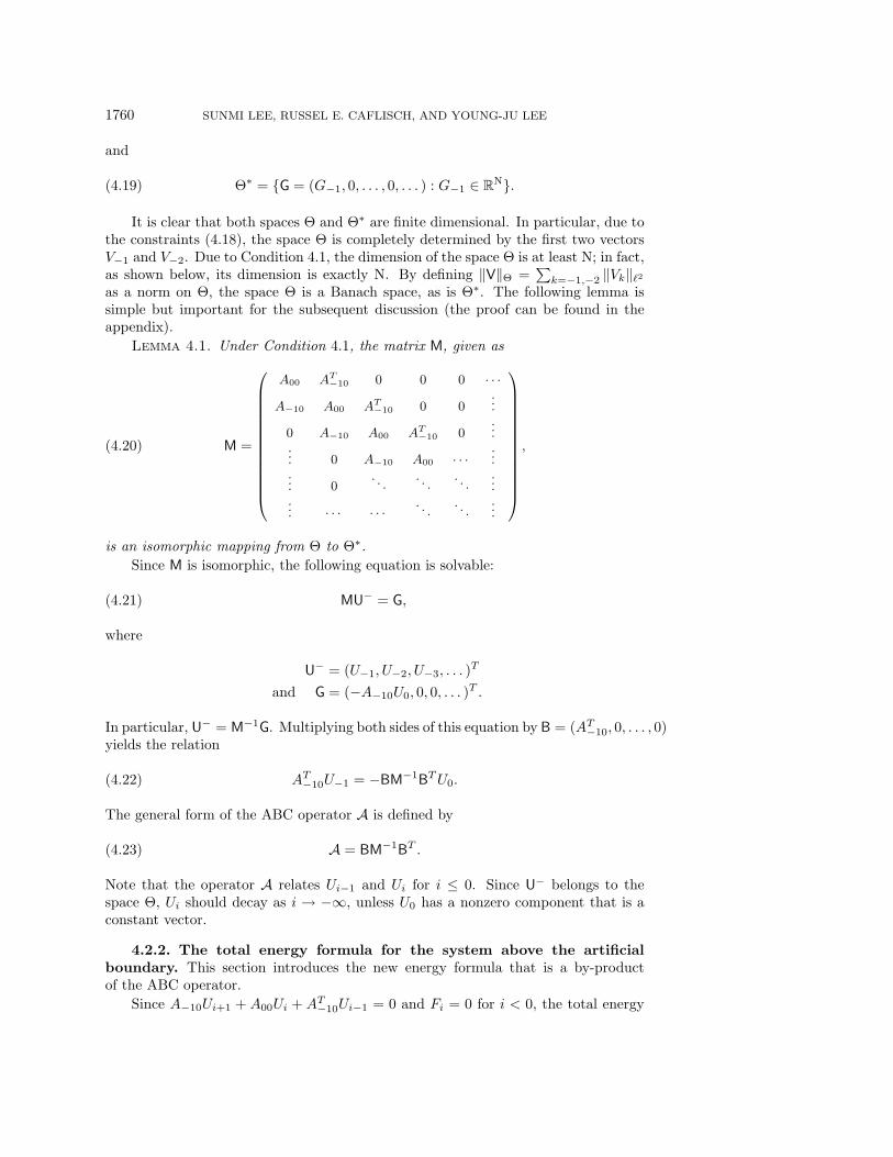
Lemma 4.1. Under Condition 4.1, the matrix M, given as

M =

⎛⎜⎜⎜⎜⎜⎜⎜⎜⎜⎜⎜⎜⎜⎝

A00 AT−10 0 0 0 · · ·

A−10 A00 AT−10 0 0

...

0 A−10 A00 AT−10 0

...... 0 A−10 A00 · · ·

...... 0

. . .. . .

. . ....

... · · · · · ·. . .

. . ....

⎞⎟⎟⎟⎟⎟⎟⎟⎟⎟⎟⎟⎟⎟⎠

,(4.20)

is an isomorphic mapping from Θ to Θ∗.

Since M is isomorphic, the following equation is solvable:

MU− = G,(4.21)

where

U− = (U−1, U−2, U−3, . . . )T

and G = (−A−10U0, 0, 0, . . . )T .

In particular, U− = M−1G. Multiplying both sides of this equation by B = (AT−10, 0, . . . , 0)

yields the relation

AT−10U−1 = −BM−1BTU0.(4.22)

The general form of the ABC operator A is defined by

A = BM−1BT .(4.23)

Note that the operator A relates Ui−1 and Ui for i ≤ 0. Since U− belongs to thespace Θ, Ui should decay as i → −∞, unless U0 has a nonzero component that is aconstant vector.

4.2.2. The total energy formula for the system above the artificialboundary. This section introduces the new energy formula that is a by-productof the ABC operator.

Since A−10Ui+1 + A00Ui + AT−10Ui−1 = 0 and Fi = 0 for i < 0, the total energy


Etotal from (4.8) can be written as follows:

Etotal =∑i≥0

1

2(Ui, (Aii+1Ui+1 + AiiUi + Aii−1Ui−1)) − (Ui, Fi)

=1

2

(U0,

(A01U1 + A00U0 + AT

−10U−1

))− (U0, F0)

+∑i>0

1

2(Ui, (Aii+1Ui+1 + AiiUi + Aii−1Ui−1)) − (Ui, Fi) .

This formula, however, depends on the displacement field U−1 below the artificialboundary. To remove this dependence and obtain an energy formula (and a reducedforce balance equation) that involves displacement fields only above the artificialboundary, use the operator A to obtain the following alternative formula:

Etotal =1

2(U0, (A01U1 + (A00 −A)U0)) − (U0, F0)(4.24)

+∑i>0

1

2(Ui, (Aii−1Ui−1 + AiiUi + Aii+1Ui+1)) − (Ui, Fi) .

Note that the energy formula given in (4.24) depends only on the displacement fieldsU0 and U+ above the artificial boundary, but it includes the energy in the strain fieldbelow the artificial boundary. In addition, optimization of this formula for the energyyields the reduced equation on the upper domain with the ABC using the operatorA, as shown in the next subsection.

4.2.3. The force balance equation. Define the following admissible solutionspace for the optimization problem (4.10):

V =

{V = (Vn, . . . , V0, V−1, . . . ) : inf

ξ∈R

‖V + ξ1‖�2 < ∞, Ψ(Vi) = 0 ∀i < 0

}.

Thanks to Condition 4.1, the force balance equation that results from minimizing thetotal energy in its reduced form (4.24) is

H

(U+

U0

)=

(AII AT

I0

AI0 A00 −A

)(U+

U0

)=

(F+

F0

).(4.25)

The reduced form (4.25) of the force balance equation, as well as its properties, isthe main result of this work. Note that (4.25) involves the Schur complement of thematrix A00 in the original force balance equation (4.13).

The properties of the matrices A and H are summarized in the following lemma,whose proof is provided in the appendix.

Lemma 4.2. The matrix A is symmetric and positive definite, the matrix H issymmetric and nonnegative definite, and the null space of H consists of the constantdisplacement fields span{1k : k = 1, 2, 3}.

The analysis in this section is performed for the Neumann boundary conditionat the top boundary Γ1, by which we mean that the variational principle (4.10)involves no constraint on the solution at Γ1. In this case, it is most important tonote that (4.25) is solvable since (F+, F0) belongs to the range of H; namely, (F+, F0)

is orthogonal to the constant vector fields, which is exactly the null space of H asnoted in Lemma 4.2. In addition, the solution to (4.25) is determined up to a constant


vector. However, the additional contribution of the constant vector does not affect thetotal energy evaluation since the total energy is invariant with respect to the constantdisplacement. Furthermore, use of the Neumann condition is only to simplify theanalysis. It does not affect the ABC operator A, which can be used for any choice ofboundary conditions on the top.

In passing to the next section, we summarize the most important properties ofthe ABC operator A, which guide its construction.P1 The operator A is a symmetric and positive definite matrix mapping R

N to RN .

P2 The relation between U−1 and U0 is that U−1 = −(AT−10)

−1AU0 = CU0.

4.3. Validation of the solvability requirement, Condition 4.1. In thissection, Condition 4.1 is derived by introducing a sum-of-exponentials ansatz. Muchof the derivation, including the most crucial steps, is analytic, but some steps arebased on numerical evidence. In related work on the Laplace equation, Hagstrom andKeller [11] performed a completely analytic validation of the analogue of Condition4.1.

The following presentation is mostly based on the thesis of Lee [18] and is similarto the work by Russo and Smereka [20], which used the palindromic eigenvalue prob-lem [15, 16]. Although these works did not state a general solvability condition likeCondition 4.1, their analysis is equivalent to a validation of this condition. Through-out this section, denote F and F−1 to be the discrete forward and backward Fouriertransforms, respectively.

4.3.1. Two dimensional case. The force balance equations at a point (xm, yi) =(m, i) are

−(Lu)1 = −C11D+x D

−x u− C44D

+y D

−y u− (C12 + C44)D

0yD

0xv = 0,(4.26)

−(Lu)2 = −C44D+x D

−x v − C11D

+y D

−y v − (C12 + C44)D

0xD

0yu = 0.

Since the solution is periodic in the x-direction, we introduce the following ansatz:

u(m, i) =1

Nx

Nx−1∑μ=0

u(μ, i) e2πıμm/Nx(4.27)

=1

Nx

Nx−1∑μ=0

u(μ)γi e2πıμm/Nx ,

where Nx is such that u(m, i) = u(Nx + m, i) for all m.From (4.27), the force balance equations (4.26) become

P (μ, γ)u(μ, i) =(γ2A−10(μ) + γA00(μ) + AH

−10(μ))u(μ, i) = 0(4.28)

for μ = 0, 1, . . . , Nx − 1, where

A−10(μ) =

(−C44 −ıC12+C44

2sin(2πμ/Nx)

−ıC12+C442

sin(2πμ/Nx) −C11

),

A00(μ) =

(2C44 + 2C11(1 − cos(2πμ/Nx)) 0

0 2C11 + 2C44(1 − cos(2πμ/Nx))

),

and AH−10 is the complex transpose of the matrix A−10.


Nontrivial solutions for this system require that

detP (μ, γ) = 0.(4.29)

This is the well-known palindromic eigenvalue problem [15, 16, 20]. Note that forμ = 0, which corresponds to the constant vector in the Fourier expansion of thesolution ansatz (4.27), the only solution to (4.29) is γ = 1, which corresponds to theconstant solution to (4.14).

For μ = 0, (4.29) has four solutions that occur in pairs (γk, γ−1k ) for k = 1, 2,

since

det(P (μ, γ)) = 0 ⇐⇒ det(P (μ, γ)) = 0(4.30)

and

P (μ, γ) = γ2P (μ, γ −1).

We then pick a pair of solutions (γ1, γ2) with |γk| > 1 for k = 1, 2, which are therelevant choices since the corresponding solution is decaying as i → −∞ for μ = 0, andwe also pick two linearly independent eigenvectors q1(μ) and q2(μ) that correspondto γ1 and γ2, respectively [10, 20]; i.e.,

P (μ, γ1)q1(μ) = P (μ, γ2)q2(μ) = 0.(4.31)

It is possible that |γk| = 1 or that γ1 = γ2 and there is a generalized eigenvector,but these possibilities have not been seen numerically. Indeed, the occurrence of ageneralized eigenvector in the continuous case (cf. section 3.2) does not seem to haveconsequences for the discrete case.

We then arrive at the general solution for u(μ, i) given as follows:

u(μ, i) = q1(μ)γi1 + q2(μ)γi

2.(4.32)

For the zero mode μ = 0, two linearly independent vectors qk(0) are q1 = (1, 0)T

and q2 = (0, 1)T . Note that omitting this mode would make 0 an eigenvalue for theoperator A, but that A should be positive definite as indicated in property P1 insubsection 4.2.3.

4.3.2. Three dimensional case. As in the two dimensional case, consider theforce balance equations at a point (xm, yn, zi) = (m,n, i):

−(Lu)1 = −C11D+x D

−x u− C44(D

+y D

−y u + D+

z D−z u)(4.33)

−(C12 + C44)(D0yD

0xv + D0

zD0xw)

= 0,

−(Lu)2 = −C11D+y D

−y v − C44(D

+x D

−x v + D+

z D−z v)

−(C12 + C44)(D0yD

0xu + D0

zD0yw)

= 0,

−(Lu)3 = −C11D+z D

−z w − C44(D

+x D

−x w + D+

y D−y w)

−(C12 + C44)(D0zD

0xu + D0

zD0yv)

= 0.


Introduce the solution ansatz as follows:

u(m,n, i) =1

NxNy

Nx−1∑μ=0

Ny−1∑ν=0

u(μ, ν, i) e(2πıμm)/Nx+(2πıνn)/Ny(4.34)

=1

NxNy

Nx−1∑μ=0

Ny−1∑ν=0

u(μ, ν)γi e(2πıμm)/Nx+(2πıνn)/Ny ,

where Nx and Ny are the periods in x and y for u. From ansatz (4.34), the forcebalance equations become

P (μ, ν, γ)u(μ, ν, i)(4.35)

=(γ2A−10(μ, ν) + γA00(μ, ν) + AH

−10(μ, ν))u(μ, ν, i) = 0

for each μ = 0, 1, . . . , Nx and ν = 0, 1, . . . , Ny, where A−10 = A−10(μ, ν) and A00 =

A00(μ, ν) are given by

A−10 =

⎛⎝ −C44 0 −s1

0 −C44 −s2

−s1 −s2 −C11

⎞⎠,

A00 =

⎛⎝ a11 a12 0

a21 a22 00 0 a33

⎞⎠,

in which

s1 = ıC12 + C44

2sin(2πμ/Nx),

s2 = ıC12 + C44

2sin(2πν/Ny)

and

a11 = 2C11(1 − cos(2πμ/Nx)) + 2C44(1 − cos(2πν/Ny)) + 2C44,

a12 = −(C12 + C44) sin(2πμ/Nx) sin(2πν/Ny),

a21 = a12,

a22 = 2C44(1 − cos(2πμ/Nx)) + 2C11(1 − cos(2πν/Ny)) + 2C44,

a33 = 2C44(1 − cos(2πμ/Nx)) + 2C44(1 − cos(2πν/Ny)) + 2C11.

A nontrivial solution can be found only if

detP (μ, ν, γ) = 0.(4.36)

As in the two dimensional case, for μ = ν = 0, the only solution is γ = 1, and for(μ, ν) = (0, 0), there are three pairs of eigenvalues, namely (γk, γ

−1k ) with |γk| > 1

for k = 1, 2, 3, and corresponding eigenvectors qk(μ, ν) that are mutually linearlyindependent, from which the general solution can be given as follows:

u(μ, ν, i) = q1(μ, ν)γi1 + q2(μ, ν)γi

2 + q3(μ, ν)γi3.(4.37)


Note that if the three values γk are distinct, then it can be seen directly that there existthree linearly independent eigenvectors qk(μ, ν) corresponding to the three eigenvaluesγk (see the appendix). Often in our computation, as seen in the work by Russo andSmereka [20], it happens that γk = γ� with k = �. When this happens, it is difficult toestablish analytically the existence of linearly independent eigenvectors; this is alwaysfound to be the case, however, in the numerical computations.

4.4. On the discrete ABC operator A and Condition 4.1. In this section,the ABC operator A is constructed for the three dimensional case only, since thetwo dimensional construction is similar but simpler. We first construct the operatorC that relates Ui−1 and Ui by Ui−1 = CUi, as indicated in P2. We then constructA = −(AT

−10)C. Finally, we discuss the validation of Condition 4.1.

Note that the Fourier transforms A−10 and A00 of A−10 and A00 consist of 3× 3

block matrices A−10(μ, ν) and A00(μ, ν). Since the vectors qi(μ, ν) from (4.37) aremutually independent, define the following mutually orthonormal vectors:

qi = ci(qi′ × qi′′),

in which each triple (i, i′, i′′) is a rearrangement of (1, 2, 3) and the constants ci’s arechosen so that

qi · qj = δij for i, j = 1, 2, 3.(4.38)

It follows that

u(μ, ν, k − 1) = C(μ, ν)u(μ, ν, k),(4.39)

in which

C(μ, ν) =

⎛⎝ qT

1

qT2

qT3

⎞⎠

−1 ⎛⎝ γ−1

1 qT1

γ−12 qT

2

γ−13 qT

3

⎞⎠ .(4.40)

The matrix C is

C = F−1CF ,(4.41)

in which

C = diag(C(μ, ν))μ=0,...,Nx−1,ν=0,...,Ny−1.(4.42)

To construct the ABC operator A, multiply −AH−10(μ, ν) by C(μ, ν). Note that

A = F−1AF , where A is a diagonal block matrix consisting of the submatricesA(μ, ν) = −AH

−10(μ, ν)C(μ, ν) for μ = 0, . . . , Nx − 1 and ν = 0, . . . , Ny − 1, namely,

A = diag(A(μ, ν))μ=0,...,Nx−1, ν=0,...,Ny−1,(4.43)

and also for both two and three dimensional cases, the operator A = F−1AF issymmetric and positive definite. It is quite difficult to see this directly from theFourier analysis discussed in this section, but it follows from the variational principlebased on the general form of the ABC operator as discussed in section 4.2.


Finally, Condition 4.1 can be validated from the construction of the matrix C.For any data U0 ∈ R

N which consists of displacement u on the interface i = 0, thevectors Ui for all i < 0 can be written as follows:

Ui = F−1CiFU0 = CiU0.(4.44)

The matrix C is invertible. It satisfies (4.17), because |γ| > 1 for (μ, ν) = 0, while for(μ, ν) = 0, γ = 1 and the corresponding term in (4.34) has no dependence on m andn, so that (4.16) is also satisfied. This completes the validation of Condition 4.1.

4.5. Total energy. In this section we derive alternative general energy formulasthat involve a product of stress and strain. Note that in the section 4.2, the energyand the variational principle are written in terms of displacement times force. Forsome applications, such as a heteroepitaxial thin film, as described in section 5.3, itis much more convenient to write the energy in the form of stress times strain, as in(4.3).

The analysis of this section relies on the following “summation by parts” formulas:

∑j≤0

(D+f)jgj = f1g0 −∑j≤0

fj(D−g)j ,(4.45)

∑j≤0

(D−f)jgj = f0g1 −∑j≤0

fj(D+g)j ,(4.46)

∑j≤0

(D0f)jgj =1

2(f1g0 + f0g1) −

∑j≤0

fj(D0g)j ,(4.47)

where D+, D−, and D0 are the forward, backward, and centered finite differenceoperators, respectively. The total energy can be decomposed into two parts:

Etotal = Ei≥0 + Ei≤−1,(4.48)

where Ei≥0 =∑

i≥0 Ei and Ei≤−1 =∑

i≤−1 Ei, and i = 0 is the layer in which theABCs are imposed. Use (4.45)–(4.47) to derive the following relations, in two andthree space dimensions, respectively:

Ei≤−1 =∑i1

αv0(D+y v)−1 + βu0(D

+y u)−1(4.49)

+∑i1

αv−1(D−y v)0 + βu−1(D

−y u)0

+∑i1

[β(u0(D

0xv)−1 + u−1(D

0xv)0)

+ γ(v0(D

0xu)−1 + v−1(D

0xu)0

)]−

∑i1,i≤−1

1

2ui · (Lui) − ui · fi

and


Ei≤−1 =∑i1,i2

αw0(D+z w)−1 + β(u0(D

+z u)−1 + v0(D

+z v)−1)(4.50)

+∑i1,i2

αw−1(D−z w)0 + β(u−1(D

−z u)0 + v−1(D

−z v)0)

+∑i1,i2

[β(v0(D

0yw)−1 + v−1(D

0yw)0 + u0(D

0xw)−1 + u−1(D

0xw)0

)+ γ

(w0(D

0yv)−1 + w−1(D

0yv)0 + w−1(D

0xu)0 + w0(D

0xu)−1

)]−

∑i1,i2,i≤−1

1

2ui · (Lui) − ui · fi,

in which L is the operator introduced in (4.26) and (4.33) and fi is the force. In theseformulas, the subscript refers to the depth-like index i.

Due to the assumption that fi = 0 for i ≤ −1, the last terms are zero in both thetwo and three dimensional cases. This leads to the following formulas:

Etotal = Ei≥0 +∑i1

αv0(D+y v)−1 + βu0(D

+y u)−1(4.51)

+∑i1

αv−1(D−y v)0 + βu−1(D

−y u)0

+∑i1

[β(u0(D

0xv)−1 + u−1(D

0xv)0)

+ γ(v0(D

0xu)−1 + v−1(D

0xu)0

)]in two dimensions and

Etotal = Ei≥0 +∑i1,i2

αw0(D+z w)−1 + β(u0(D

+z u)−1 + v0(D

+z v)−1)(4.52)

+∑i1,i2

αw−1(D−z w)0 + β(u−1(D

−z u)0 + v−1(D

−z v)0)

+∑i1,i2

[β(v0(D

0yw)−1 + v−1(D

0yw)0 + u0(D

0xw)−1 + u−1(D

0xw)0

)+ γ

(w0(D

0yv)−1 + w−1(D

0yv)0 + w−1(D

0xu)0 + w0(D

0xu)−1

)]in three dimensions. In both (4.51) and (4.52), we replace U−1 by CU0 whenever u−1

appears.If the ABCs are imposed on the layer i = 0 where there is no force, then the total

energy could be computed by the following new energy formulas that do not involveU−1 or the operator C:

Etotal = Ei>0 +∑i1

αv1(D+y v)0 + βu1(D

+y u)0(4.53)

+∑i1

αv0(D−y v)1 + βu0(D

−y u)1

+∑i1

[β(u1(D

0xv)0 + u0(D

0xv)1)

+ γ(v1(D

0xu)0 + v0(D

0xu)1

)]


in two space dimensions and

Etotal = Ei>0 +∑i1,i2

αw1(D+z w)0 + β(u1(D

+z u)0 + v1(D

+z v)0)(4.54)

+∑i1,i2

αw0(D−z w)1 + β(u0(D

−z u)1 + v0(D

−z v)1)

+∑i1,i2

[β(v1(D

0yw)0 + v0(D

0yw)1 + u1(D

0xw)0 + u0(D

0xw)1

)+ γ

(w1(D

0yv)0 + w0(D

0yv)1 + w0(D

0xu)1 + w1(D

0xu)0

)]in three space dimensions, respectively. In both (4.53) and (4.54), we replace U−1 by−(AT

−10)−1AU0 whenever u−1 appears.

5. Numerical results. In this section, sample computations are performed tovalidate and illustrate the ABCs developed in previous sections. Throughout thissection, the elastic constants C11, C12, C44 are assumed to be C11 = 8, C12 = 4, andC44 = 4 unless explicitly stated otherwise.

5.1. The ABCs for continuum elasticity. This section shows the effective-ness of the ABCs for continuum elasticity equations (3.7). The Lame constants arechosen to be λ = 1 and τ = 1.

The test problem is (3.7) on Ω = [0, 2π)×(−∞, 0) with data on Γ1 = [0, 2π)×{y =0}. Periodicity is assumed in the lateral direction, and there is no body force; i.e.,f = 0. The interface Γ2 at which the artificial boundary condition is imposed is theline [0, 2π) × {y = −1}.

The Dirichlet data given on Γ1 is as follows:

u = (u, v) = (cosx + sin 2x, 0),

for which the exact solution to (3.7) is

(5.1)

u =

((1 +

y

2

)cosx ey + (1 + y) sin 2x e2y,

7

2sinx ey − y cos 2x e2y

).

This exact solution is compared to the solution of (3.7) with the exact artificial bound-ary condition (3.16) on the interface Γ2 and also to the solutions with the followingtwo alternative boundary conditions:

• The zero Dirichlet boundary condition u(x,−1) = 0.• The Neumann boundary condition n · T = 0 on y = −1.

Figure 5.1 shows the u-displacement field at the line y = −0.75 for the exact solution,the solution using ABCs, and the two alternative solutions. Although there is stillerror, due to discretization of the continuum equation, it is clear that the solutionobtained with the exact ABCs (3.16) is in good agreement with the analytic solu-tion (5.1). On the other hand, the solutions obtained with the other two boundaryconditions are in error by about 20%–30% at the peaks.

5.2. The ABCs for discrete elasticity. In this section, we investigate theABCs for the discrete elastic equations for both two and three space dimensions withthe Dirichlet data given on the boundary Γ1. As in the continuum case, there are noexternal forces, and periodic boundary conditions are imposed in the lateral directions.


0 1 2 3 4 5 6 7−0.5

−0.4

−0.3

−0.2

−0.1

0

0.1

0.2

0.3

0.4

0.5Displacement u

x

u

ABCexactZeroBCNeumann

Fig. 5.1. Test of the ABCs for the continuum solution in two space dimensions. Comparisonof the u-displacement field of u = (u, v) given at y = −0.75 for the exact solution (line) and for thefollowing boundary conditions: ABC (circle), zero-displacement (plus), and Neumann (triangle).

0 5 10 15 20 25−1.5

−1

−0.5

0

0.5

1

1.5Displacement u

x

u


Fig. 5.2. Test of the exact discrete ABCs in two dimensions: a comparison of the u-displacement field of u = (u, v) at (x, y) = (x, 3). The boundary Γ1 is at y = 1, and the interface Γ2

is at y = 5 for the exact solution (line) and for the following boundary conditions: ABC (circle),zero-displacement (plus), and Neumann (triangle).

More precisely, for the two dimensional case, the lattice Ω consists of Nx = 25layers in the x-direction and Ny = 5 in the y-direction, and the prescribed Dirichletboundary condition for u on Γ1 = {y = 1} is

u = (cosx + sin 2x, sinx).(5.2)

For the three dimensional case, the lattice Ω consists of Nx = Ny = 25 layers in thex- and y-directions and Nz = 4 layers in the z-direction, and the Dirichlet data onΓ1 = {z = 1} is

u = (cosx + sin 2x, sin y, sinx).(5.3)

Numerical results are plotted in Figures 5.2 and 5.3. For numerical experiments,the exact ABCs and other approximate boundary conditions are imposed on Γ2 ={y = 5} for the two dimensional case and Γ2 = {z = 4} for the three dimensionalcase, respectively. The results show that the solution with the ABCs is much moreaccurate than those from the Dirichlet and Neumann boundary conditions. Indeed,the accuracy obtained with the ABCs operator is within the round-off error, i.e.,O(10−14).

5.3. Numerical simulations for thin films. In heteroepitaxial growth, a thinfilm of one material (e.g., Ge) is grown on top of a substrate of a second material (e.g.,Si), with perfect, single crystalline structure in both materials and with the lattice


0 2 4 6 8 10 12 14 16 18 20−0.8

−0.6

−0.4

−0.2

0

0.2

0.4

0.6

0.8Displacement v

y

v


Fig. 5.3. Test of the exact discrete ABCs in three dimensions: a comparison of the v-displacement field of u = (u, v, w) at (x, y, z) = (10, y, 3). The boundary Γ1 is at z = 1, andthe interface Γ2 is at z = 4 for the exact solution (line) and for the following boundary conditions:ABC (circle), zero-displacement (square), and Neumann (triangle).

structure of the film determined by the substrate. If the lattice constants af and asfor the film and substrate are different (e.g., aGe = 1.04×aSi), then strain is generatedin the film. This strain has important effects on the material structure, as well as onits electronic properties.

For this system, it is most convenient to define the atomic displacement relativeto a single reference lattice, for example, the equilibrium lattice of the substrate, sothat the displacement u in the film is defined relative to a nonequilibrium referencelattice. The bond displacement dk± is then

dk±(i) = (dk±1 , dk±2 , dk±3 ) = D±k u(i) − εekχ,(5.4)

in which ε =af−as

asis the relative lattice displacement, and χ is 0 in the substrate

and 1 in the film. The resulting discrete strain equations have a force of size ε alongthe film/substrate interface, and the energy has the form

Etotal =1

2(HU,U) − (F,U) + G(ε),(5.5)

where

(F,U) =∑i

∑p=±,k=1,2,3

εDpkukχ.(5.6)

Further details are given, for example, in [5].In this section, we compare the displacement fields u that are computed with the

ABCs and with zero boundary conditions for a heteroepitaxial thin film. Since theforces lie on the film/substrate boundary, the artificial boundary can be taken to beany plane below this interface. Our computational domain is three dimensional withΓ2 being of size 10 × 10. As in the last section, we denote NC to be the thicknessof the substrate, including Γ2. Note that on the top boundary Γ1, the homogeneousNeumann boundary condition (no external force) is imposed.

To demonstrate the effectiveness of the ABCs, we first compute the displacementfield u by imposing the ABCs on Γ2 with substrate thickness NC = 1 and take it asthe reference solution. We then compute two displacement fields that are generatedby imposing zero boundary conditions on the bottom boundary with NC = 2 andNC = 8. For these three solutions, Figure 5.4 shows a comparison of the u component


1 2 3 4 5 6 7 8 9 10

−8

−6

−4

−2

0

x 10−4 Displacement u at x=1

y

u

ABC2 layers with 0 BC8 layers with 0 BC

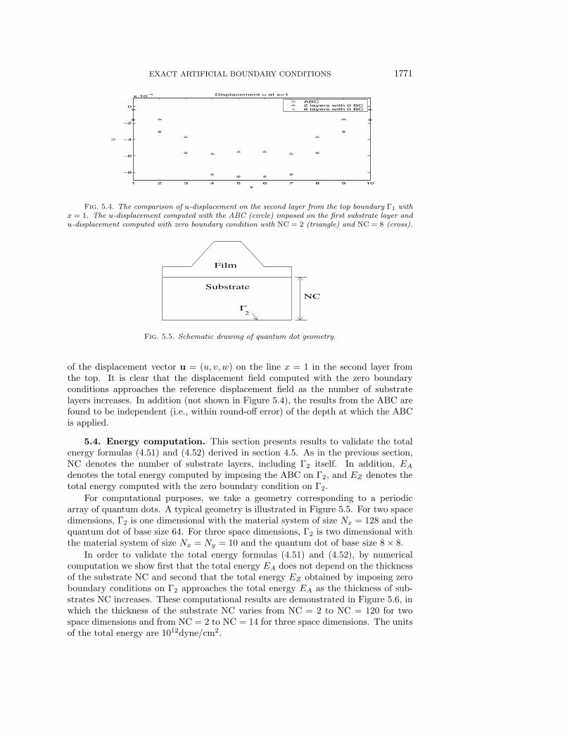
Fig. 5.4. The comparison of u-displacement on the second layer from the top boundary Γ1 withx = 1. The u-displacement computed with the ABC (circle) imposed on the first substrate layer andu-displacement computed with zero boundary condition with NC = 2 (triangle) and NC = 8 (cross).

Film

NCSubstrate

Γ

2

Fig. 5.5. Schematic drawing of quantum dot geometry.

of the displacement vector u = (u, v, w) on the line x = 1 in the second layer fromthe top. It is clear that the displacement field computed with the zero boundaryconditions approaches the reference displacement field as the number of substratelayers increases. In addition (not shown in Figure 5.4), the results from the ABC arefound to be independent (i.e., within round-off error) of the depth at which the ABCis applied.

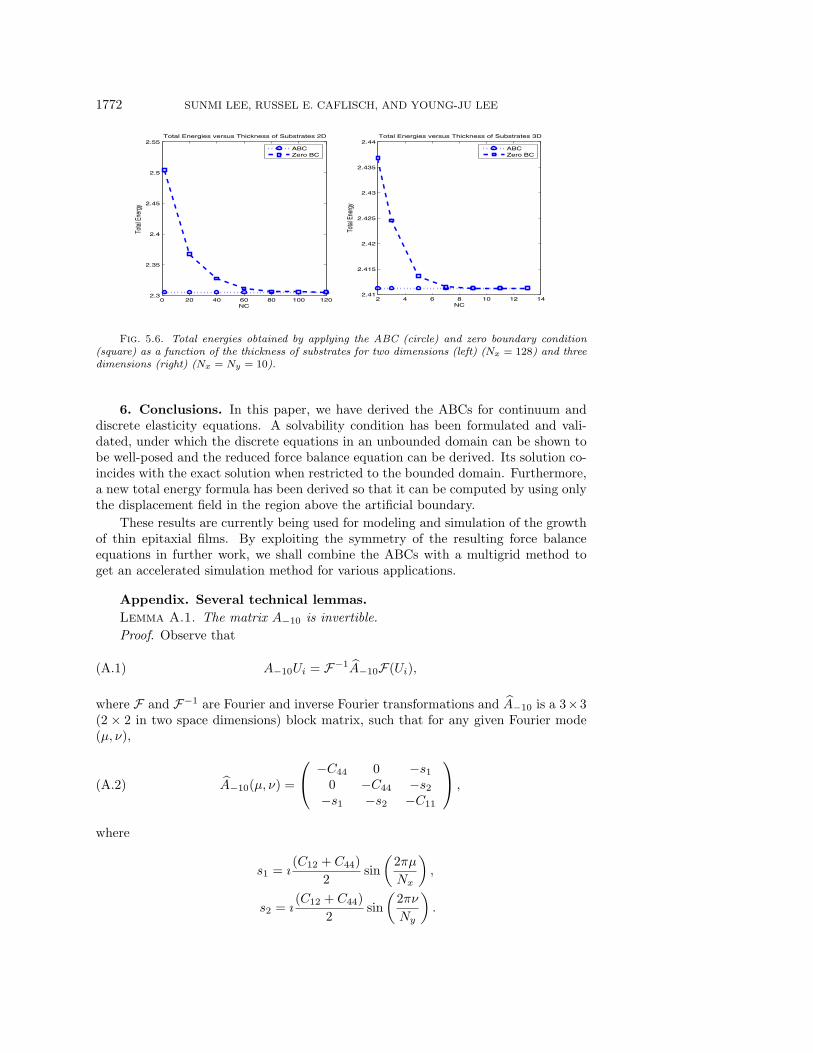
5.4. Energy computation. This section presents results to validate the totalenergy formulas (4.51) and (4.52) derived in section 4.5. As in the previous section,NC denotes the number of substrate layers, including Γ2 itself. In addition, EA

denotes the total energy computed by imposing the ABC on Γ2, and EZ denotes thetotal energy computed with the zero boundary condition on Γ2.

For computational purposes, we take a geometry corresponding to a periodicarray of quantum dots. A typical geometry is illustrated in Figure 5.5. For two spacedimensions, Γ2 is one dimensional with the material system of size Nx = 128 and thequantum dot of base size 64. For three space dimensions, Γ2 is two dimensional withthe material system of size Nx = Ny = 10 and the quantum dot of base size 8 × 8.

In order to validate the total energy formulas (4.51) and (4.52), by numericalcomputation we show first that the total energy EA does not depend on the thicknessof the substrate NC and second that the total energy EZ obtained by imposing zeroboundary conditions on Γ2 approaches the total energy EA as the thickness of sub-strates NC increases. These computational results are demonstrated in Figure 5.6, inwhich the thickness of the substrate NC varies from NC = 2 to NC = 120 for twospace dimensions and from NC = 2 to NC = 14 for three space dimensions. The unitsof the total energy are 1012dyne/cm2.


0 20 40 60 80 100 1202.3

2.35

2.4

2.45

2.5

2.55

NC

Tota

l Ene

rgy

Total Energies versus Thickness of Substrates 2D

2 4 6 8 10 12 142.41

2.415

2.42

2.425

2.43

2.435

2.44Total Energies versus Thickness of Substrates 3D

NC

Tota

l Ene

rgy

ABCZero BC

ABCZero BC

Fig. 5.6. Total energies obtained by applying the ABC (circle) and zero boundary condition(square) as a function of the thickness of substrates for two dimensions (left) (Nx = 128) and threedimensions (right) (Nx = Ny = 10).

6. Conclusions. In this paper, we have derived the ABCs for continuum anddiscrete elasticity equations. A solvability condition has been formulated and vali-dated, under which the discrete equations in an unbounded domain can be shown tobe well-posed and the reduced force balance equation can be derived. Its solution co-incides with the exact solution when restricted to the bounded domain. Furthermore,a new total energy formula has been derived so that it can be computed by using onlythe displacement field in the region above the artificial boundary.

These results are currently being used for modeling and simulation of the growthof thin epitaxial films. By exploiting the symmetry of the resulting force balanceequations in further work, we shall combine the ABCs with a multigrid method toget an accelerated simulation method for various applications.

Appendix. Several technical lemmas.

Lemma A.1. The matrix A−10 is invertible.

Proof. Observe that

A−10Ui = F−1A−10F(Ui),(A.1)

where F and F−1 are Fourier and inverse Fourier transformations and A−10 is a 3×3(2 × 2 in two space dimensions) block matrix, such that for any given Fourier mode(μ, ν),

A−10(μ, ν) =

⎛⎝ −C44 0 −s1

0 −C44 −s2

−s1 −s2 −C11

⎞⎠ ,(A.2)

where

s1 = ı(C12 + C44)

2sin

(2πμ

Nx

),

s2 = ı(C12 + C44)

2sin

(2πν

Ny

).


The eigenvalues for A−10(μ, ν) can be obtained by solving the following equation:

det(A−10(μ, ν) − λI) = −(C44 + λ)[(C44 + λ)(C11 + λ) − s2

1 − s22

](A.3)

= −(C44 + λ)[λ2 + (C11 + C44)λ + C11C44

+ sin2(2πμ/Nx)(C12 + C44)2/4

+ sin2(2πν/Ny)(C12 + C44)2/4

].

Hence, three eigenvalues λ1, λ2, and λ3 are given as follows:

λ1 = − C44,

2λ2 = − (C11 + C44)

+√

(C11 − C44)2 − (sin2(2πμ/Nx) + sin2(2πν/Ny))(C12 + C44)2,

2λ3 = − (C11 + C44)

−√

(C11 − C44)2 − (sin2(2πμ/Nx) + sin2(2πν/Ny))(C12 + C44)2.

The eigenvalue with the smallest magnitude is λ2 with sin(2πν/Nx) = sin(2πμ/Ny) =0, in which case

2λ2 = (−(C11 + C44) + |C11 − C44|) = −2 min(C11, C44).(A.4)

It follows that no eigenvalues can be zero; hence A−10 is invertible. This completesthe proof.

Lemma A.2. For γi = γj, the corresponding eigenvectors qi and qj are linearlyindependent.

Proof. Consider the linear reformulation of the palindromic eigenvalue problem(4.30) by introducing x = γy as follows: With P (μ, ν, γ) = γ2A−10 + γA00 + AH

−10,(0 I

−AH−10 −A00

)(yx

)= γ

(I 0

0 A−10

)(yx

).(A.5)

From the fact that A−10 is invertible, it is obvious that the eigenvectors qi and qj

that correspond to different eigenvalues γi and γj must be linearly independent.Lemma A.3. Under Condition 4.1, the matrix M given in (4.20) is an isomorphic

mapping from Θ to Θ∗.Proof. For V− = (V−1, V−2, . . . )

T ∈ Θ with Vi = CiV0 for i ≤ 0, as in Condition4.1,

MV− = (−A−10V0, 0, . . . , 0, . . . )T(A.6)

= G = (G−1, 0, . . . , 0, . . . )T

if G−1 = −A−10V0. Since A−10 is invertible, this shows that the matrix M is onto.To show that M is one to one, it is enough to show that MV− = 0 implies V− = 0.

Consider the energy

E− =∑i<0

Ei(A.7)

over the space Θ and observe that

(MV−,V−) = E−,(A.8)


in which E− is E− for V0 = 0. Therefore, MV− = 0 implies that E− = 0. Connectivityof the lattice and U0 = 0 then imply that Ui = 0 for all i < 0. This shows that thematrix M is one to one. Therefore, M : Θ �→ Θ∗ is isomorphic.

Proof of Lemma 4.2.First, we show that A is symmetric. For any U = (0, 0, . . . , 0, U0, U−1, . . . , . . . )

T

and V = (0, 0, . . . , 0, V0, V−1, . . . , . . . )T that belong to the space V, Condition 4.1

implies that

AT−10V−1 = −AV0 and AT

−10U−1 = −AU0.(A.9)

Note also that E(U,V) = E(V,U); i.e.,

E(U,V) =1

2

(U0,

(A00V0 + AT

−10V−1

))(A.10)

=1

2

(V0,

(A00U0 + AT

−10U−1

))= E(V,U).

Use (A.9) in (A.11) to obtain

(U0, (A00V0 −AV0)) = (V0, (A00U0 −AU0)) .

Since A00 is symmetric, this implies that (U0,AV0) = (V0,AU0) for all U0, V0 ∈ RN

and therefore, that A is symmetric. The symmetry of the operator A implies thatthe matrix H is symmetric.

Next, we show that A is positive definite since for U0 = 0 ∈ RN ,

(U0,AU0) = (U0,BM−1BTU0) = (BTU0,M−1BTU0)

= (MU−,M−1MU−) = (MU−,U−) = E− > 0,

where U− is the unique solution of MU− = BTU0. Finally, we show that the matrixH is nonnegative definite. First note that H1 = 0. Furthermore, there is no othernull space for H, since

H

(U+

U0

)= 0 ⇐⇒ (U0, (A01U1 + (A00 −A)U0))

+∑i>0

(Ui, (Aii−1Ui−1 + AiiUi + Aii+1Ui+1)) = 0

⇐⇒ E(U,U) = 0 with U ∈ V

⇐⇒ U = 1 by connectivity of the lattice.

This completes the proof of Lemma 4.2.

Acknowledgment. The authors wish to thank the anonymous referees whoseremarks helped us to improve our manuscript.

REFERENCES

[1] C. R. Anderson, The Application of Domain Decomposition to the Solution of Laplace’sEquation in Infinite Domains, CAM Report 87–19, University of California at Los Angeles,Los Angeles, 1987.

[2] X. Antoine, C. Besse, and S. Descombes, Artificial boundary conditions for one-dimensionalcubic nonlinear Schrodinger equations, SIAM J. Numer. Anal., 43 (2006), pp. 2272–2293.

[3] A. Bayliss, M. Gunzburger, and E. Turkel, Boundary conditions for the numerical solu-tions of elliptic equations in exterior regions, SIAM J. Appl. Math., 42 (1982), pp. 430–451.


[4] R. E. Caflisch, Y.-J. Lee, S. Shu, Y. Xiao, and J. Xu, An application of multigrid methodsfor a discrete elastic model for epitaxial systems, J. Comput. Phys., to appear.

[5] C. Connell, R. E. Caflisch, E. Luo, and G. D. Simms, The elastic field of a surface step:The Marchenko–Parshin formula in the linear case, J. Comput. Appl. Math, to appear.

[6] M. Ehrhardt, Finite difference schemes on unbounded domains, in Advances in the Applica-tions of Nonstandard Finite Difference Schemes, Vol. 2, World Scientific, Hackensack, NJ,2005, pp. 343–384.

[7] D. Givoli, Numerical Methods for Problems in Infinite Domains, Elsevier, Amsterdam, 1992.[8] D. Givoli and J. B. Keller, Nonreflecting boundary conditions for elastic waves, Wave Mo-

tion, 12 (1990), pp. 261–279.[9] D. Givoli, I. Patlashenko, and J. B. Keller, High-order boundary conditions and finite

elements for infinite domains, Comput. Methods Appl. Mech. Engrg., 143 (1997), pp.13–39.

[10] G. H. Golub and C. F. Van Loan, Matrix Computations, The Johns Hopkins UniversityPress, Baltimore, MD, 1996.

[11] T. Hagstrom and H. B. Keller, Exact boundary conditions at an artificial boundary forpartial differential equations in cylinders, SIAM J. Math. Anal., 17 (1986), pp. 322–341.

[12] H. Han and W. Bao, Error estimates for the finite element approximation of linear elasticequations in an unbounded domain, Math. Comp., 70 (2000), pp. 1437–1459.

[13] H. Han, W. Bao, and T. Wang, Numerical simulation for the problem of infinite elasticfoundation, Comput. Methods Appl. Mech. Engrg., 147 (1997), pp. 369–385.

[14] H. Han and X. Wu, The approximation of the exact boundary conditions at an artificialboundary for linear elastic equations and its application, Math. Comp., 59 (1992), pp.21–37.

[15] A. Hilliges, C. Mehl, and V. Mehrmann, On the solution of palindromic eigenvalue prob-lems, in Proceedings of the European Congress on Computational Methods in AppliedSciences and Engineering (ECCOMAS), 2004.

[16] M. E. Hochstenbach and H. A. van der Vorst, Alternatives to the Rayleigh quotient forthe quadratic eigenvalue problem, SIAM J. Sci. Comput., 25 (2003), pp. 591–603.

[17] L. D. Landau and E. M. Lifshitz, Theory of Elasticity, Butterworth-Heinemann, Oxford,UK, 1986.

[18] S. Lee, Artificial Boundary Conditions for Linear Elasticity and Atomistic Strain Models,Ph.D. thesis, University of California at Los Angeles, Los Angeles, 2005.

[19] P. G. Martinsson and I. Babuska, Mechanics of materials with periodic truss or framemicro-structures I: Korn’s inequality, in Arch. Ration. Mech. Anal., to appear.

[20] G. Russo and P. Smereka, Computation of strained epitaxial growth in three dimensions bykinetic Monte Carlo, J. Comput. Phys., 214 (2006), pp. 809–828.

[21] A. Schindler, M. F. Gyure, G. D. Simms, D. D. Vvendensky, R. E. Caflisch, C. Connell,

and E. Luo, Theory of strain relaxation in heteroepitaxial systems, Phys. Rev. B, 67 (2003),no. 075316.

exact artificial boundary conditions for continuum and discrete...

Documents