HAL Id: hal-00122640https://hal.archives-ouvertes.fr/hal-00122640v2

Preprint submitted on 4 Jan 2007

HAL is a multi-disciplinary open accessarchive for the deposit and dissemination of sci-entific research documents, whether they are pub-lished or not. The documents may come fromteaching and research institutions in France orabroad, or from public or private research centers.

L’archive ouverte pluridisciplinaire HAL, estdestinée au dépôt et à la diffusion de documentsscientifiques de niveau recherche, publiés ou non,émanant des établissements d’enseignement et derecherche français ou étrangers, des laboratoirespublics ou privés.

Exact and efficient interpolation using finite elementsshape functions

Gustavo Silva, Rodolphe Le Riche, Jérôme Molimard, Alain Vautrin

To cite this version:Gustavo Silva, Rodolphe Le Riche, Jérôme Molimard, Alain Vautrin. Exact and efficient interpolationusing finite elements shape functions. 2007. �hal-00122640v2�

Exact and efficient interpolation using finite elementsshape functions

G.H.C. Silva, R. Le Riche, J. Molimard and A. Vautrin

Ecole Nationale Superieure des Mines de Saint-Etienne, France158, cours Fauriel F-42023 Saint-Etienne cedex 2

January 4, 2007

Abstract

The increasing use of finite elements (FE) and optical full-field measurement methods have con-tributed to the growing need to compare mesh-based degrees of freedom with experimental fields ofdiscrete data points. Applying generic interpolation algorithms (e.g. using linear, cubic and B-splineweight functions) creates a dependency of the interpolated field to non-physical parameters that may af-fect high-frequency information through implicit filtering and introduces fundamental assumptions to theshape of experimental data field. The alternative is to use the existing FE mesh and shape functions todetermine mesh degrees of freedom at each experimental data point. This comparison technique makesno assumptions beyond those already made in the FE model. In this sense, interpolation using elementshape functions is exact. However, this approach requires calculating the local FE coordinates of theexperimental points (inverse mapping), which is non-trivial and not a standard part of FE software.

Basic implementations of FE interpolation can be time consuming and impractical for applicationsrequiring the comparison of large fields to be repeated several times. This article analyzes a two-stepprocess for FE interpolation. First the element containing a given data point is determined, then theinterpolation inside the element using reference coordinates. An efficient strategy is proposed, whichrelies on cross-products, element bounding-boxes and a multi-dimensional storage array (virtual mesh).The strategy yields a linear computation cost with respects to the number of elements in the FE mesh andnumber of data points in the experimental field, contrary to a quadratic cost from standard approaches. Asample application is given using a plate with a hole.

Contents1 Introduction 2

2 Overview of interpolation techniques 32.1 General interpolation . . . . . . . . . . . . . . . . . . . . . . . . . . . . . . . . . . . . . 32.2 Methods based on finite elements shape functions . . . . . . . . . . . . . . . . . . . . . . 3

2.2.1 Projection of data points onto FE response space . . . . . . . . . . . . . . . . . . 42.2.2 FE interpolation at data points . . . . . . . . . . . . . . . . . . . . . . . . . . . . 4

3 Determination of the owner element 53.1 Element tests . . . . . . . . . . . . . . . . . . . . . . . . . . . . . . . . . . . . . . . . . 5

3.1.1 Cross-product test . . . . . . . . . . . . . . . . . . . . . . . . . . . . . . . . . . 53.1.2 Bounding-box test . . . . . . . . . . . . . . . . . . . . . . . . . . . . . . . . . . 5

3.2 Searching the element list . . . . . . . . . . . . . . . . . . . . . . . . . . . . . . . . . . . 63.3 Comparison of owner element search algorithms . . . . . . . . . . . . . . . . . . . . . . . 7

4 Inverse mapping 84.1 Analytic inverse mapping for QUAD4 elements . . . . . . . . . . . . . . . . . . . . . . . 104.2 Iterative inverse mapping . . . . . . . . . . . . . . . . . . . . . . . . . . . . . . . . . . 11

5 Numerical experiments 12

6 Conclusions 14

A Search time details for QUAD4 elements 16

1

B Inverse mapping theorems 19

C Selecting the virtual mesh grid size 22

D Pseudo code for search algorithms 23

Summary of notatione(p) An element containing p.ε(p) A neighborhood around point p.nj

i The ith node of set j.nmesh The set of nodes in a finite elements mesh.nε(p) Set of nodes in a neighborhood of p.Ne Number of elements in a finite element’s mesh.Np Number of points in in the data field.N cl Average number bounding-boxes that claim an arbitrary data point.Nk Average number of finite elements in a virtual element.Nve Average number of virtual elements which share a reference to a finite element.p A data point.p A set of data points.STi Search Technique i.T , T Time measured in CPU seconds and number of operations, respectively.Tb Build time or pre-processing time.Tc Time complexity.Tf Failure time.Ti Search time for a data point belonging to the ith element in a sequential list.Ts Success time.Tt Total search time.TX |Y Time factor X for search technique Y.~v A vector.vi The ith scalar component of vector ~v.~x(p) Coordinates of point p in the global coordinate system.~ξ(p) Coordinates of point p in an element’s reference coordinate system.

1 IntroductionThe increasing use of finite elements has given rise to a series of applications requiring the comparisonof discrete data fields with finite elements results. These applications include mesh-interaction [4, 22],geological topography [10], visualization [16, 20], calibration of boundary conditions [17] and materialidentification [5, 7, 9, 11, 12, 14, 15]. In general, a finite elements solver provides information only atnodal or integration points. Available data points may not always coincide with mesh points, and before acomparison can be performed, it is necessary to map one field of points onto the other.

Three types of mapping techniques can be employed for this purpose: node placement, where FE nodesand experimental points are forced to coincide [7, 14], approximation and interpolation 1 [8, 13, 12]. Sincethe accuracy of the FE models is a function of node position, node placement techniques introduce an un-desired coupling between the position of data points and the accuracy of the finite elements model. Genericinterpolation and approximation algorithms (ex. using linear, cubic and B-spline weight functions) createsa dependency of the interpolated field to non-physical parameters that may eliminate high-frequency in-formation through implicit filtering, and introduces fundamental assumptions to the shape of experimentaldata field. This article presents interpolation techniques using FE shape functions. This approach was se-lected over other mapping techniques because it makes no assumptions other than those already introducedin the finite elements model. The strategies discussed in this article consist of two parts: First, the elementcontaining each data point (the owner element) is identified. Next, the coordinates of the data point are

1Unlike interpolation, approximation points do not necessarily match experimental or FE data points.

2

transformed into the finite element’s reference coordinate system (hereafter this procedure is referred to asinverse mapping). The reference coordinates are used to compute the element’s shape-function coefficientswhich perform the interpolation.

Many of the cited applications require the interpolation of anywhere from 1×103 to 1×106 data pointsto be repeated several thousand times [15]. Hence, it is very important that this mapping be carried out asquickly, accurately and reliably as possible. To address this demand, the article analyzes a series of tech-niques to reduce the number of operations required for interpolation of large data fields. These techniquesconsist of different search methods for the owner element (including the cross-product and bounding-boxtests, and the virtual mesh), and inverse mapping methods (including analytical and iterative methods). Webegin with a description of the different search algorithms, followed by a theoretical estimation in com-putational cost. Since the search time is dependent on the exact mesh configuration, the algorithms arebench-marked using meshes of 2D 4-nodes quadrilateral elements (QUAD4). Using the theoretical esti-mates, the algorithm with the lowest computational cost is determined. A C++ implementation of thesealgorithms is used to support the theoretical estimates on a plate with a hole problem.

2 Overview of interpolation techniquesThis section presents a brief overview of the possible techniques for comparing discrete data fields with FEresults.

2.1 General interpolationThe griddata function in the Matlab software package [13] provides four techniques to obtain data u(p)at arbitrary points p from a cloud of mesh data u(nmesh): triangle-based linear, cubic, nearest neighborand biharmonic spline (B-spline) interpolation. All of these techniques except B-spline [21] generate in-terpolation meshes via Delaunay triangulation [3]. A triangle defines a zone of influence for interpolationcoefficients Wi, where

u(p) =no. nodes in ε(p)∑

i=1

Wi

(~x(p), ~x(nε(p))

)u(nε(p)

i ). (1)

The nearest-node and linear interpolation algorithms are the fastest, but have discontinuous zeroth andfirst derivatives, respectively. The other two are continuous up to the second derivatives, but are significantlyslower. In addition, griddata does not account for fields with an internal discontinuity, such as a plate witha hole. The algorithm fills the hole with elements, thus introducing boundary effects on the interpolateddata. Kriging [8] is another popular interpolation approach popular in geo-statistics. It has the advantage ofproviding an estimation of the interpolation variance. However, it is computationally expensive (requiringthe solution of a large linear system for each data point). Another drawback of general interpolation is thatthey affect the data by introducing non-physical parameters to the comparison (i.e., kernel width, polynomialdegrees, variogram length and scales in kriging).

2.2 Methods based on finite elements shape functionsWith FE shape functions, Nj , the value u(p) is estimated from the node values u(ne(p)) of the elementcontaining the data point p, e(p) (hereafter referred to as the owner element),

u(p) =no. nodes in e(p)∑

j=1

Nj

(~ξ(p)

)u(ne(p)

j ). (2)

Notice that in general shape functions are written in the reference system of the element containing pointp. Calculating the local coordinates of a point is not a trivial operation, requiring two steps. First, findingthe owner element. Second, calculating the local coordinates of the point (an operation referred to asinverse mapping), which in general involves solving a multi-dimension non-linear system of equations. Thecomparison of the FE model and data fields is performed either at the coordinates of the FE nodes or datapoints. Continuity is guaranteed for the zeroth derivative, but is generally discontinuous for higher-orderderivatives.

3

0 0.2 0.4 0.6 0.8 10.1

0.2

0.3

0.4

0.5

0.6

0.7

0.8

0.9

Delaunay Triangulation

x

y

(a) Nodes

0 0.2 0.4 0.6 0.8 10.1

0.2

0.3

0.4

0.5

0.6

0.7

0.8

0.9

Delaunay Triangulation

x

y

(b) Interpolation Mesh

−2

0

2

−2

0

2−0.5

0

0.5

x

Linear Interpolation

y

z

(c) Linear Interpolation

−2

0

2

−2

0

2−0.5

0

0.5

x

Nearest Node

y

z

(d) Nearest Node Approximation

Figure 1: Interpolation using the Matlab griddata function.

2.2.1 Projection of data points onto FE response space

E. Pagnacco and D. Lemosse [18] describe a technique where the data field is approximated at the nodal co-ordinates of the finite elements mesh. The method searches for node values u(nmesh) that best fit availabledata u′(p). The approximation is defined as the projection of the data onto the finite elements model space.The values of u(nmesh) are determined by solving a least-squares problem,

minu(nmesh)

no. points in p∑i=1

u′(pi)−no. nodes in ε(pi)∑

j=1

Nj

(~ξ(pi)

)u(ne(p)

j )

2

. (3)

This technique requires a number of data points greater than the number of finite elements nodes, andthat the data field encompass a representative part of the finite elements mesh. The computational costinvolves determining the reference coordinates of each data point, and solving the least-squares problem.For applications where the comparison is performed multiple times over a non-changing finite elementsmesh, the interpolation of the data points has to be performed only once. This projection method mayeliminate (filter) high-frequency information in the measurement (e.g. experimental noise).

2.2.2 FE interpolation at data points

Instead of interpolating measured data points at FE node coordinates, this article selects the interpolationof data from nodes at the coordinates of the experimental points, leaving the experimental data unaltered.The strategy consists of simply evaluating equation (2) for each data point, p ∈ p. A special effort ismade to improve the speed of determining the owner element. This approach allows for the computationof degrees of freedom at arbitrary points, and has no restriction in the distribution or the number of datapoints. The FE solution is completely independent of the position and size of the experimental data field,and since the same mesh is used for solving the model and interpolating the data, the resulting interpolatedfield is an exact representation of the FE solution. Also, similar to the previous technique, the interpolationcoefficients can be computed only once for a non-changing mesh, thus saving time on applications thatrepeat the interpolation several times. Different from the previous technique, this approach does not performimplicit filtering, thus allowing for the consideration of high-frequency information.

4

3 Determination of the owner elementInterpolation using shape functions is accomplished in three steps: the determination of the element con-taining the data point (owner element), the transformation of the data point’s coordinates into the referencecoordinate system (inverse mapping), and finally the application of the finite elements shape functions todetermine the degrees of freedom at that point (equation (2)). The determination of the owner element is notrequired to be an elaborated step in the algorithm. The program could attempt sequentially inverse mappinga point for every element in the mesh. Using the reference coordinates the program can check if the pointfalls inside the domain of the element (section 4). However, since inverse mapping may be complex andnumerically expensive, such an approach would be inefficient. Moreover, inverse mapping algorithms arenot guaranteed to have a solution for points outside the element’s domain, which affects the reliability ofa two-step interpolation algorithm. Instead, a combination of simple tests is used to determine the ownerelement before performing the inverse mapping.

3.1 Element testsThis section describes the cross-product and bounding-box tests. The term “element test” refers to anytechnique to determine whether a point lies inside or outside of an element.

3.1.1 Cross-product test

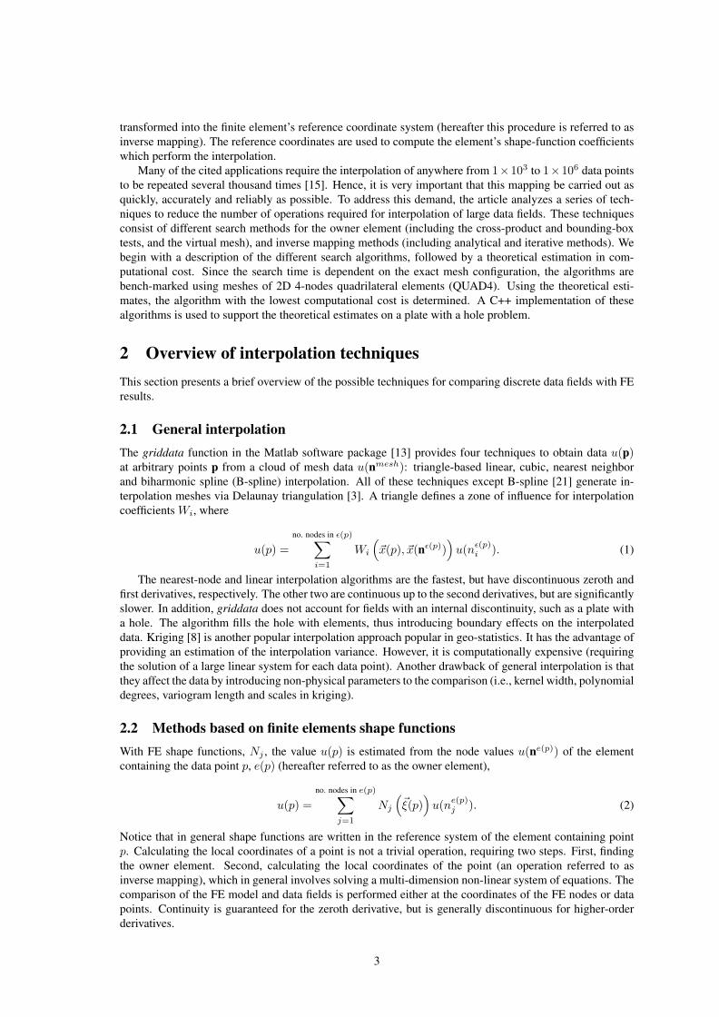
The cross-product test (Figure 2(a)) consists in a series of cross and dot products, which determines if adata point lies inside the intersection of the “vertex cones” of an element. The approach is equivalent totechniques described by P. Burke [6]. If point p is inside the element, then for every node, n ∈ ne(p), thevector ~np will lie inside the cone created by the two adjacent node vectors, ~ni and ~nj. This condition ischecked using the vectors ~s1 and ~s2,

~s1 = ~ni× ~np

and ~s2 = ~np× ~nj.(4)

These vectors will point in the same direction for internal points and in opposite directions for externalpoints. Hence, an internal point must satisfy the condition

~s1 · ~s2 ≥ 0 (5)

for all nodes in the element. If a point lies outside the element, there is at least one vertex such that

~s1 · ~s2 < 0. (6)

The cross-product test requires that a spatially ordered list of nodes be available for each element (this isstandard in finite elements mesh formats). This test is exact for elements with linear edges, and approximateotherwise.

3.1.2 Bounding-box test

The bounding-box test creates an encompassing box around the finite element [19] and compares the coor-dinates of the data point with the bounding-box’s two opposite corner points, pmin and pmax (see Figure2(b)). The coordinates of any point inside the bounding-box must satisfy the inequality

xi(pmin) ≤ xi(pinternal) ≤ xi(pmax) (7)

for all dimensions i. At least one of the inequalities will be false for an external point. The complexity ofthe test includes two parts: computing the boundaries of the bounding-box (later stored in memory), andtesting if a data point lies inside the bounding-box. Since the bounding-box only approximates the geometryof a finite element, it is possible for a point to be inside the bounding-box, but outside the finite element(pinternal in Figure 2(b)). Thus, in order to identify the owner element, it is necessary for the bounding-boxtest to be used together with an exact test such as the cross-product test. Section 3.3, discusses the advan-tages of scanning a list of finite elements using the bounding-box and cross-product tests together insteadof a search algorithm using only the cross-product test. The algorithm first eliminates impossible owner

5

(a) Cross-Product Test (b) Bounding-Box Test

Figure 2: (a) The cross-product test uses cross and dot products to check if a point lies inside all vertexcones of an element. (b) The bounding-box test uses a rectangular approximation of the element to quicklyeliminate impossible owner elements (case of external points).

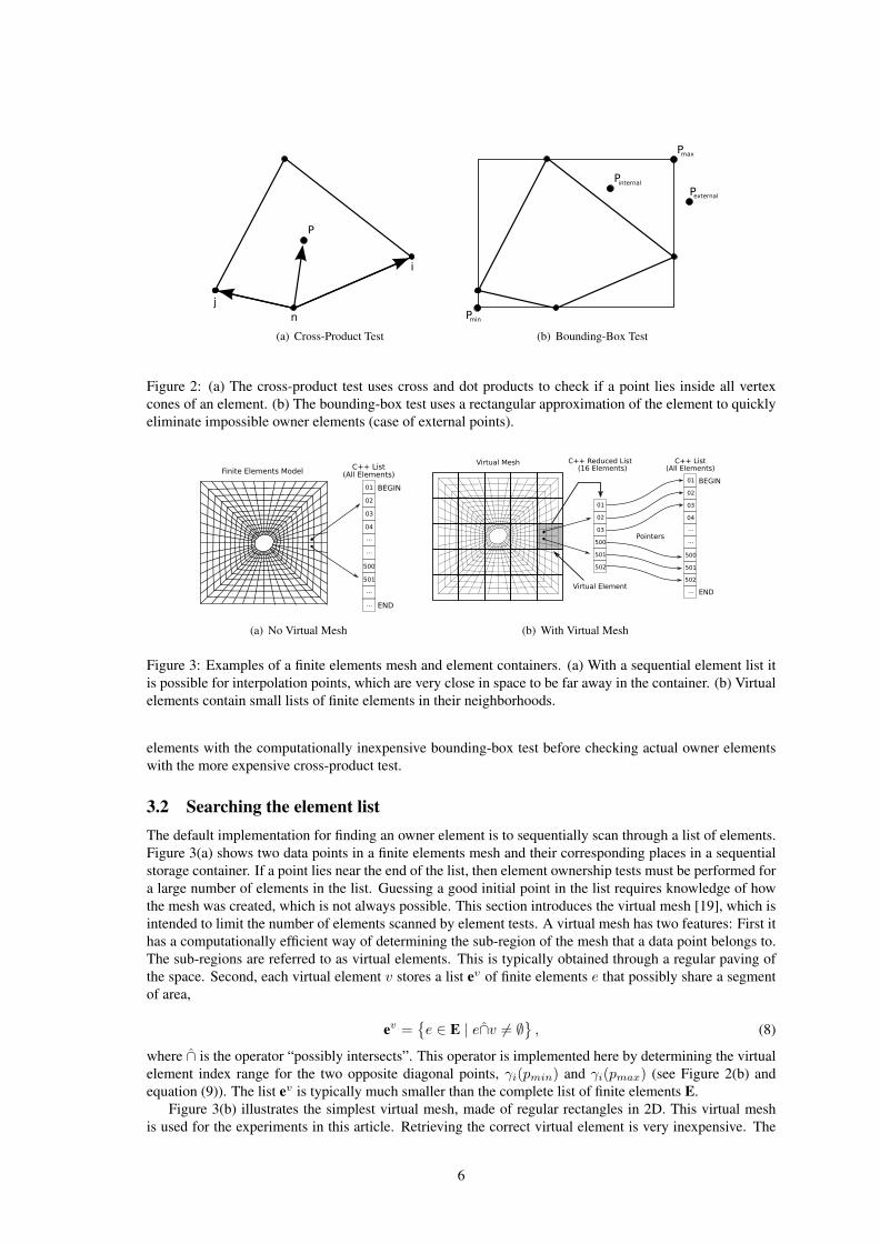
(a) No Virtual Mesh (b) With Virtual Mesh

Figure 3: Examples of a finite elements mesh and element containers. (a) With a sequential element list itis possible for interpolation points, which are very close in space to be far away in the container. (b) Virtualelements contain small lists of finite elements in their neighborhoods.

elements with the computationally inexpensive bounding-box test before checking actual owner elementswith the more expensive cross-product test.

3.2 Searching the element listThe default implementation for finding an owner element is to sequentially scan through a list of elements.Figure 3(a) shows two data points in a finite elements mesh and their corresponding places in a sequentialstorage container. If a point lies near the end of the list, then element ownership tests must be performed fora large number of elements in the list. Guessing a good initial point in the list requires knowledge of howthe mesh was created, which is not always possible. This section introduces the virtual mesh [19], which isintended to limit the number of elements scanned by element tests. A virtual mesh has two features: First ithas a computationally efficient way of determining the sub-region of the mesh that a data point belongs to.The sub-regions are referred to as virtual elements. This is typically obtained through a regular paving ofthe space. Second, each virtual element v stores a list ev of finite elements e that possibly share a segmentof area,

ev ={e ∈ E | e∩v 6= ∅

}, (8)

where ∩ is the operator “possibly intersects”. This operator is implemented here by determining the virtualelement index range for the two opposite diagonal points, γi(pmin) and γi(pmax) (see Figure 2(b) andequation (9)). The list ev is typically much smaller than the complete list of finite elements E.

Figure 3(b) illustrates the simplest virtual mesh, made of regular rectangles in 2D. This virtual meshis used for the experiments in this article. Retrieving the correct virtual element is very inexpensive. The

6

ith dimension index γi of the virtual element containing the data point p can is determined using only 3operations,

γi = floor

(xi(p)− xi

dxi

), (9)

where xi is the origin of the virtual mesh grid and dxi is the virtual mesh’s grid-step in the ith direction.Once the virtual element has been retrieved, its small list of finite elements, ev , is scanned using elementtests.

3.3 Comparison of owner element search algorithmsThis section compares three algorithms to find the owner element of a data point. Each algorithm is definedby a combination of element tests and an element retrieval technique (either sequential or based on a virtualmesh).

• Search technique 1 (ST1) sequentially scans the full list of finite elements using the cross-producttest. The process is restarted at the beginning of the list for each data point.

• Search technique 2 (ST2) is a sequential search of the full finite elements list using a combinationof the cross-product and bounding-box tests. This algorithm is essentially the same as the previoustechnique, except that the cross-product test is performed only if the data point is inside the finiteelement’s bounding box. If the element fails the bounding box test, the algorithm moves to the nextelement in the list. The idea is to eliminate impossible owner elements with the computationallyinexpensive bounding-box test before using the more expensive cross-product test.

• Search technique 3 (ST3) uses the cross-product and bounding-box tests to search small lists of finiteelements obtained with the virtual mesh. For each data point, the algorithm retrieves the appropriatevirtual element, and scans the small list of finite elements using a test similar to ST2.

The efficiency of an element search algorithm is estimated by counting average number of operations.Operations are defined as basic math operations (+ − × ÷), comparison operations (= 6= < > 6 >),assignment operations and standard mathematical functions in the C library. A finite element programcontaining a sequential list of Ne elements as illustrated in Figure 3. The search time for a data pointbelonging to the ith element in this list is

Ti = (i− 1)× Tf + Ts, (10)

where Ts (success time) and Tf (failure time) are the computation times (measured in number of operations)to determine that the data point does or does not belong to an element, respectively. Assuming for an averagefield, that a point can belong to any element in the list with equal probability, the time complexity Tc, namelythe average number of operations to determine the owner element of one point, is

Tc(Ne) =1

Ne

Ne∑i=1

Ti. (11)

The total search time Tt is an estimate of the average number of operations required to identify the ownerelement for Np arbitrary data points including a preprocessing time Tb (required to initialize bounding boxesand the virtual mesh),

Tt(Ne, Np) = Tb(Ne) + Tc(Ne)×Np. (12)

The objective of the analysis is to determine which combination of element tests results in the smallesttotal search time, Tt. An estimate of Tt was computed for ST1, ST2 and ST3 applied to meshes of QUAD4elements. These search times are functions of the number of elements Ne the number of interpolation pointsNp as well as mesh-specific geometric parameters: A measure of mesh distortion N cl, specifically theaverage number of finite element bounding-boxes that will claim an arbitrary data point, Nve, the average

7

number of virtual elements possessing a reference to the same finite element and Nk, the average numberof finite elements in a virtual element. An approximate relationship between Nk and Nve is developed inAppendix C. It uses a coefficient α, which is the ratio of the average bounding-box area of a finite element,Ae, to the area of a virtual element, dx× dy,

α =Ae

dx× dy. (13)

The approximation considers the limiting behavior of Nk and Nve as α→ 0 and α→∞, while accountingfor and mesh to virtual mesh offsets (see Figure 14 in Appendix C),

Nk ≈1α

+ 1 (14)

and Nve ≈ α + 1. (15)

If α is very large (i.e. very small virtual elements) the majority of the virtual elements will contain thereference to only one finite element, leading to a decrease in the time complexity Tc of the search algorithm.However, since there are more virtual elements, the preprocessing time Tb will offset the advantage gainedby the smaller Tc. The ratio α∗ represents the the best compromise between Tc and Tb. It is obtained bydifferentiating Tt|st3 with respects to α and solving for a zero (see Appendix C),

α∗ =√

1.25Np

Ne. (16)

Table 1 summarizes the search times of interest, the proofs of which can be found in Appendix A.

Time Cross-Product Test Bounding-Box Test Virtual MeshTb 0 20Ne (5Ne + 7) +

[20 + Nve + 12

]Ne

Tf 37.5 2.5 Does Not ApplyTs 60 4 Does Not Apply

Search Technique Computation TimeST1 Tt|st1 = 18.75NeNp + 41.25Np

ST2 Tt|st2 = 1.25NeNp + 20.75N clNp + 110.5Np + 20Ne

ST3 Tt|st3 = (Nve + 37)Ne +[1.25Nk + 20.75N cl + 116.5

]Np + 7

Table 1: Computation times

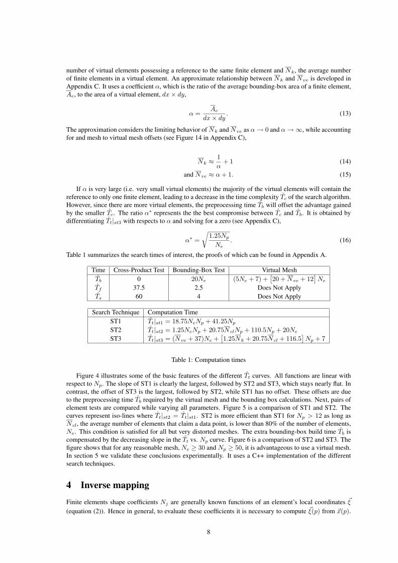
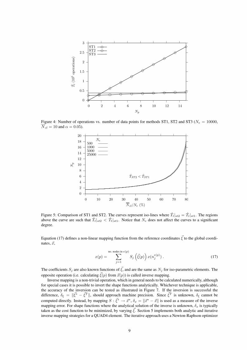
Figure 4 illustrates some of the basic features of the different Tt curves. All functions are linear withrespect to Np. The slope of ST1 is clearly the largest, followed by ST2 and ST3, which stays nearly flat. Incontrast, the offset of ST3 is the largest, followed by ST2, while ST1 has no offset. These offsets are dueto the preprocessing time Tb required by the virtual mesh and the bounding box calculations. Next, pairs ofelement tests are compared while varying all parameters. Figure 5 is a comparison of ST1 and ST2. Thecurves represent iso-lines where Tt|st2 = Tt|st1. ST2 is more efficient than ST1 for Np > 12 as long asN cl, the average number of elements that claim a data point, is lower than 80% of the number of elements,Ne. This condition is satisfied for all but very distorted meshes. The extra bounding-box build time Tb iscompensated by the decreasing slope in the Tt vs. Np curve. Figure 6 is a comparison of ST2 and ST3. Thefigure shows that for any reasonable mesh, Ne ≥ 30 and Np ≥ 50, it is advantageous to use a virtual mesh.In section 5 we validate these conclusions experimentally. It uses a C++ implementation of the differentsearch techniques.

4 Inverse mapping

Finite elements shape coefficients Nj are generally known functions of an element’s local coordinates ~ξ

(equation (2)). Hence in general, to evaluate these coefficients it is necessary to compute ~ξ(p) from ~x(p).

8

0

0.5

1

1.5

2

2.5

3

0 2 4 6 8 10 12 14

Tt(1

05op

erat

ions)

Np

ST1ST2ST3

Figure 4: Number of operations vs. number of data points for methods ST1, ST2 and ST3 (Ne = 10000,N cl = 10 and α = 0.05).

0

2

4

6

8

10

12

14

16

18

20

0 10 20 30 40 50 60 70 80

Np

N cl/Ne (%)

TST2 < TST1

Ne

5001000500025000

Figure 5: Comparison of ST1 and ST2. The curves represent iso-lines where Tt|st2 = Tt|st1. The regionsabove the curve are such that Tt|st2 < Tt|st1. Notice that Ne does not affect the curves to a significantdegree.

Equation (17) defines a non-linear mapping function from the reference coordinates ~ξ to the global coordi-nates, ~x,

x(p) =no. nodes in e(p)∑

j=1

Sj

(~ξ(p)

)x(ne(p)

j ) . (17)

The coefficients Sj are also known functions of ~ξ, and are the same as Nj for iso-parametric elements. Theopposite operation (i.e. calculating ~ξ(p) from ~x(p)) is called inverse mapping.

Inverse mapping is a non-trivial operation, which in general needs to be calculated numerically, althoughfor special cases it is possible to invert the shape functions analytically. Whichever technique is applicable,the accuracy of the inversion can be tested as illustrated in Figure 7. If the inversion is successful thedifference, δξ = ‖~ξ∗ − ~ξT ‖, should approach machine precision. Since ~ξT is unknown, δξ cannot becomputed directly. Instead, by mapping S : ~ξ∗ → ~x∗, δx = ‖~x∗ − ~x‖ is used as a measure of the inversemapping error. For shape functions where the analytical solution of the inverse is unknown, δx is typicallytaken as the cost function to be minimized, by varying ~ξ. Section 5 implements both analytic and iterativeinverse mapping strategies for a QUAD4 element. The iterative approach uses a Newton-Raphson optimizer

9

Ne

Np

TST3 < TST2

N cl = 2015

105

1

10 20 30 40 50 60 70 80 90 100

10

20

30

40

50

60

70

80

90

100

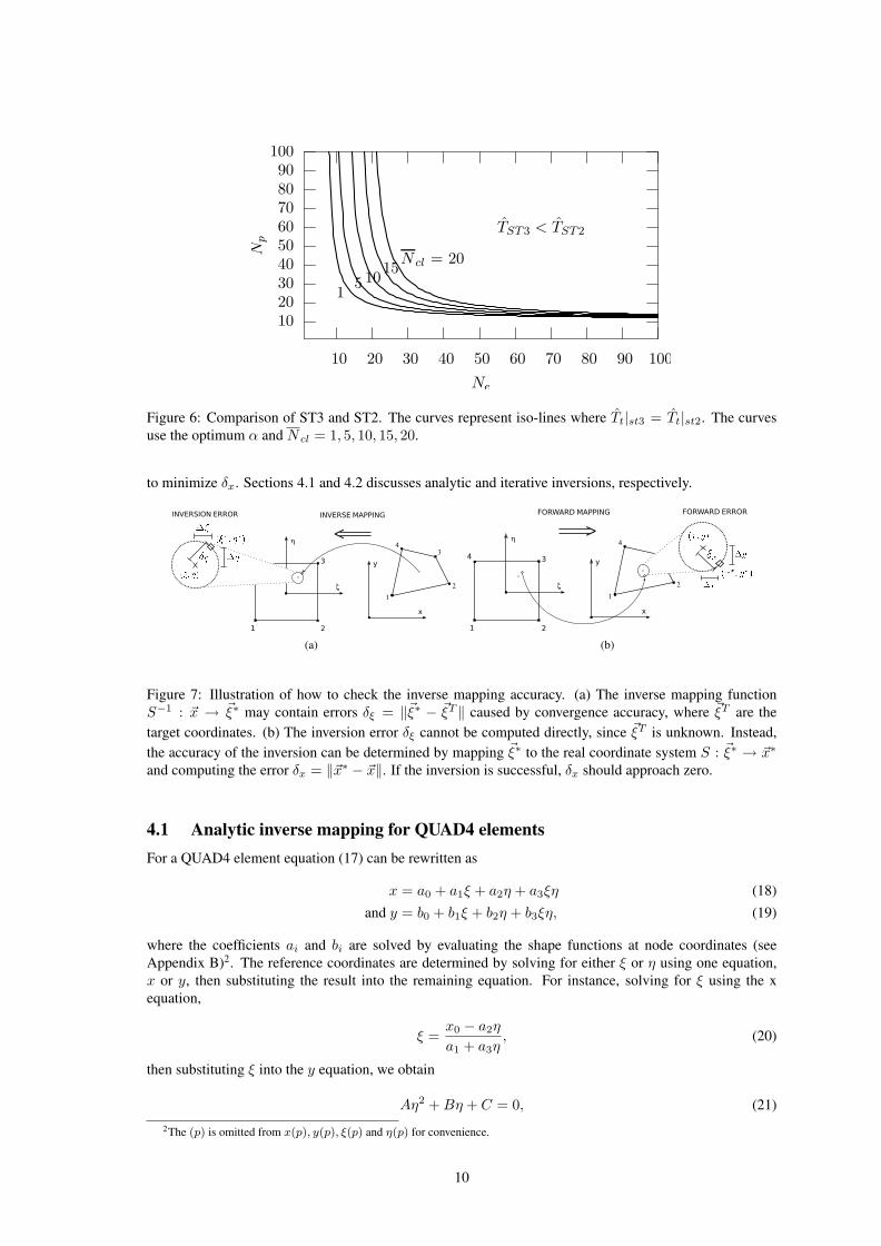
Figure 6: Comparison of ST3 and ST2. The curves represent iso-lines where Tt|st3 = Tt|st2. The curvesuse the optimum α and N cl = 1, 5, 10, 15, 20.

to minimize δx. Sections 4.1 and 4.2 discusses analytic and iterative inversions, respectively.

(a) (b)

Figure 7: Illustration of how to check the inverse mapping accuracy. (a) The inverse mapping functionS−1 : ~x → ~ξ∗ may contain errors δξ = ‖~ξ∗ − ~ξT ‖ caused by convergence accuracy, where ~ξT are thetarget coordinates. (b) The inversion error δξ cannot be computed directly, since ~ξT is unknown. Instead,the accuracy of the inversion can be determined by mapping ~ξ∗ to the real coordinate system S : ~ξ∗ → ~x∗

and computing the error δx = ‖~x∗ − ~x‖. If the inversion is successful, δx should approach zero.

4.1 Analytic inverse mapping for QUAD4 elementsFor a QUAD4 element equation (17) can be rewritten as

x = a0 + a1ξ + a2η + a3ξη (18)and y = b0 + b1ξ + b2η + b3ξη, (19)

where the coefficients ai and bi are solved by evaluating the shape functions at node coordinates (seeAppendix B)2. The reference coordinates are determined by solving for either ξ or η using one equation,x or y, then substituting the result into the remaining equation. For instance, solving for ξ using the xequation,

ξ =x0 − a2η

a1 + a3η, (20)

then substituting ξ into the y equation, we obtain

Aη2 + Bη + C = 0, (21)2The (p) is omitted from x(p), y(p), ξ(p) and η(p) for convenience.

10

where the coefficients A,B, C are

A = a3b2 − a2b3,B = (x0b3 + a1b2)− (y0a3 + a2b1),C = x0b1 − y0a1

(22)

and x0 = a0 − x, y0 = b0 − y. Thus, in general, inverse mapping requires the solution of a quadratic equa-tion. However, if equation (20) results in division by zero (i.e. a1+a3η = 0), an alternative inverse mappingformulation must be used. For geometrically admissible elements (i.e. elements wit no crossing edges anda non-zero area) two cases cover all possible situations. Details including proofs of these formulations canbe found in Appendix B.case 1, a1 6= 0, a3 6= 0 : The value of η is obtained from a1 + a3η = 0,

η =−a1

a3, (23)

and ξ by substituting η into the y equation,

ξ =y0a3 + a1b2

a3b1 − a1b3. (24)

case 2, a1 = 0 , a3 = 0 : The value of η is obtained by solving the x equation,

η =x0

a2, (25)

and ξ by substituting η into the y equation,

ξ =y0a2 − x0b2

a2b1 + x0b3. (26)

4.2 Iterative inverse mappingIn applications where the shape functions are more complex than QUAD4 elements, an analytical inversionof the shape functions may become too tedious to be carried out. Figure 8 illustrates one such case. Theelement in question is a 20 node 3D brick element, which contains a set of three 2nd order 3D shapefunctions. The alternative is to use an iterative technique to compute the reference coordinates of data pointp.

The iterative process begins with an initial guess of the reference coordinates, ~ξ0, which can be selectedfrom node coordinates, integration points, element center, or any other point inside the element. Consider aformulation of the square of the forward error, f , where ~ξT (p) and ~xT (p) are the target coordinates of p,

f(~ξ) = δ2x(~ξ) = (xT

j (p)− Si(~ξ)xj(ne(p)i ))2. (27)

Notice that both xTj (p) and xj(n

e(p)i ) are known quantities and Si are known functions of ~ξ, the unknowns.

Since the shape functions are continuous in the reference coordinate system, the function f(~ξ) must becontinuous and zero (its minimum) at the solution point ~ξT ,

f(~ξT ) = fmin = 0. (28)

Hence, it is possible to minimize f to solve for ~ξ(p). Since the shape functions are polynomials, a gradientmethod may be used for this purpose. Using this technique the condition

gi =∂f

∂ξi= 0 (29)

must be satisfied at the solution point. Hence, the iteration step is ∆~ξ = − 12H−1~g, where H is the Hessian

of f, Hij = ∂2f∂ξi∂ξj

. The individual partial derivatives are computed from equation (27),

∂f

∂ξi= 2(xT

k (p)− Sl(~ξ)xl(ne(p)k )

∂Sl(~ξ)∂ξi

,

11

(a) Reference Element

Corners:Si(ξ, η, ζ) = 1

8 (1 + ξξi)(1 + ηηi)(1 + ζζi)(ξξi + ηηi + ζζi − 2)Sides:Si(ξ, η, ζ) = 1

4 (1 + ξ2)(1 + ηηi)(1 + ζζi)

~x(p) =∑20

i=1 Si~x(ne(p)i )

(b) Shape Functions

Figure 8: A 20-node 3D brick element (BRK20)

∂2f

∂ξi∂ξj= 2

∂Sl(~ξ)∂ξi

∂Sl(~ξ)∂ξj

+ 2(xTk (p)− Sl(~ξ)xl(n

e(p)k ))

∂2Sl(~ξ)∂ξi∂ξj

.

The iteration should continue until reaching the stopping criteria, δx ≤ δallow. The stop criteria depends onthe inversion accuracy required by an application.

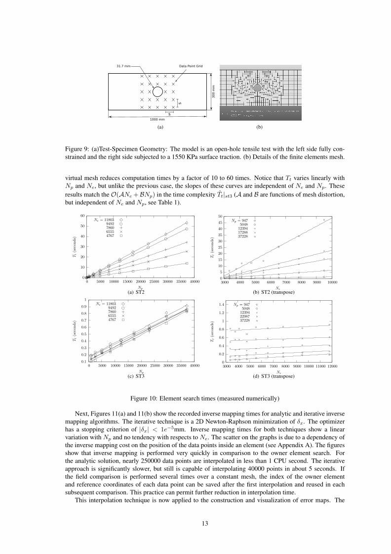
5 Numerical experimentsThe efficiency of owner element search algorithms were estimated in section 3.3 by counting operations. Itassumed that other contributions to the algorithm’s time complexity are negligible (e.g. memory allocation,different computation costs for integer and floating point arithmetic, etc). This section checks these as-sumptions by comparing the theoretical estimates with numerical experiments. The computation times aremeasured when interpolating data-point grids, with varying number of points Np over meshes of differentelement numbers Ne. The experiments are conducted with a C++ implementation of the interpolation algo-rithms, with an ABAQUS 6.4 finite elements solver [1]. The computer test-bed is a Toshiba satellite A60with a Pentium 4 processor running on a GNU/Linux Debian 3.1 operating system [2]. The FE model isan open-hole plate specimen illustrated in Figure 9. The model’s left side is fully constrained, and the rightside subjected to a 1550 KPa surface traction. The data points, p, are located on a grid of step s (Figure 9) 3.The total processing time Tt is measured by an embedded C++ timer, which measures the time in secondsfrom the beginning of the interpolation procedure until all data points in the grid have been interpolated.The procedure is repeated with different mesh sizes, Ne, and grid steps s.

Figures 10(a) and 10(b) show the test results for the ST2 algorithm, which uses the bounding-box andcross-product tests to sequentially scan the entire list of finite elements. The execution time, Tt, increaseslinearly with Ne and Np when Np and Ne are held constant. Notice that the slopes of Tt increases with Ne

and Np. The experimental behavior is in agreement with theO(Ne×Np) time complexity Tt|st2 in section3.3 (Table 1). Figure 10(c) shows the results for the ST3 algorithm, which uses a combination of the cross-product and bounding-box tests and a virtual mesh container. Clearly, the interpolation algorithm using thevirtual mesh is more efficient than the previous algorithm. For large number of points (Ne ≥ 5000), the

3The data point grids encompass only a square window on the center of the model. Since the numbering of the elements follows arectangular pattern, the square data field can be considered average.

12

(a) (b)

Figure 9: (a)Test-Specimen Geometry: The model is an open-hole tensile test with the left side fully con-strained and the right side subjected to a 1550 KPa surface traction. (b) Details of the finite elements mesh.

virtual mesh reduces computation times by a factor of 10 to 60 times. Notice that Tt varies linearly withNp and Ne, but unlike the previous case, the slopes of these curves are independent of Ne and Np. Theseresults match the O(ANe +BNp) in the time complexity Tt|st3 (A and B are functions of mesh distortion,but independent of Ne and Np, see Table 1).

0

10

20

30

40

50

60

0 5000 10000 15000 20000 25000 30000 35000 40000

Tt(s

econ

ds)

Np

Ne = 118039492786065554767

(a) ST2

0

5

10

15

20

25

30

35

40

45

50

3000 4000 5000 6000 7000 8000 9000 10000

Tt(s

econ

ds)

Ne

Np = 9475048

123941728837228

(b) ST2 (transpose)

0.1

0.2

0.3

0.4

0.5

0.6

0.7

0.8

0.9

1

0 5000 10000 15000 20000 25000 30000 35000 40000

Tt(s

econ

ds)

Np

Ne = 118039492786065554767

(c) ST3

0

0.2

0.4

0.6

0.8

1

1.2

1.4

3000 4000 5000 6000 7000 8000 9000 10000 11000 12000

Tt(s

econ

ds)

Ne

Np = 9475048

123942298737228

(d) ST3 (transpose)

Figure 10: Element search times (measured numerically)

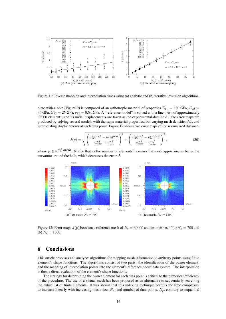
Next, Figures 11(a) and 11(b) show the recorded inverse mapping times for analytic and iterative inversemapping algorithms. The iterative technique is a 2D Newton-Raphson minimization of δx. The optimizerhas a stopping criterion of |δx| < 1e−5mm. Inverse mapping times for both techniques show a linearvariation with Np and no tendency with respects to Ne. The scatter on the graphs is due to a dependency ofthe inverse mapping cost on the position of the data points inside an element (see Appendix A). The figuresshow that inverse mapping is performed very quickly in comparison to the owner element search. Forthe analytic solution, nearly 250000 data points are interpolated in less than 1 CPU second. The iterativeapproach is significantly slower, but still is capable of interpolating 40000 points in about 5 seconds. Ifthe field comparison is performed several times over a constant mesh, the index of the owner elementand reference coordinates of each data point can be saved after the first interpolation and reused in eachsubsequent comparison. This practice can permit further reduction in interpolation time.

This interpolation technique is now applied to the construction and visualization of error maps. The

13

0

0.5

1

1.5

2

2.5

60 80 100 120 140 160 180 200 220 240

T(s

econ

ds)

Np (1× 103 points)

T = mNp + b

m = 1.4× 10−4, b = 0

Ne = 130015621728221425923324423956917834

11849

(a) Analytic inverse mapping

0

1

2

3

4

5

6

0 5 10 15 20 25 30 35 40

T(s

econ

ds)

Np (1× 103 points)

T = mNp + b

m = 1.4 × 10−4, b = 0

Ne = 1728221425923324423956917834

11849

(b) Iterative inverse mapping

Figure 11: Inverse mapping and interpolation times using (a) analytic and (b) iterative inversion algorithms.

plate with a hole (Figure 9) is composed of an orthotropic material of properties E11 = 100 GPa, E22 =36 GPa, G12 = 25 GPa, ν12 = 0.54 GPa. A “reference model” is solved with a fine mesh of approximately33000 elements, and its nodal displacements are taken as the experimental data field. The error maps areproduced by solving several models with the same material properties, but varying mesh densities Ne, andinterpolating displacements at each data point. Figure 12 shows two error maps of the normalized distance,

J(p) =

√√√√(u(p)ref − u(p)test

urefmax − uref

min

)2

+

(v(p)ref − v(p)test

vrefmax − vref

min

)2

, (30)

where p ∈ nref. mesh. Notice that as the number of elements increases the mesh approximates better thecurvature around the hole, which decreases the error J .

x (mm)

-148 -74.1 -0.0675 74 148

y (mm)

-149

-74.5

-0.00075

74.5

149

0.000171

0.00471

0.00925

0.0138

0.0183

0.0229

0.0274

0.0319

0.0365

0.041

0.0455

0.0501

0.0546

0.0592

0.0637

0.0682

J(x, y)

(a) Test mesh: Ne = 700

x (mm)

-148 -74.1 -0.0675 74 148

y (mm)

-149

-74.5

-0.00075

74.5

149

0.000171

0.00471

0.00925

0.0138

0.0183

0.0229

0.0274

0.0319

0.0365

0.041

0.0455

0.0501

0.0546

0.0592

0.0637

0.0682

J(x, y)

(b) Test mesh: Ne = 1500

Figure 12: Error maps J(p) between a reference mesh of Ne = 30000 and test meshes of (a) Ne = 700 and(b) Ne = 1500.

6 ConclusionsThis article proposes and analyzes algorithms for mapping mesh information to arbitrary points using finiteelement’s shape functions. The algorithms consist of two parts: the identification of the owner element,and the mapping of interpolation points into the element’s reference coordinate system. The interpolationis then a direct evaluation of the element’s shape functions.

The strategy for determining the owner element for each data point is critical to the numerical efficiencyof the procedure. The use of a virtual mesh has been proposed as an alternative to sequentially searchingthe entire list of finite elements. It was shown that this indexing technique permits the time complexityto increase linearly with increasing mesh size, Ne, and number of data points, Np, contrary to sequential

14

techniques, which increase quadratically with Ne ×Np. In addition to the virtual mesh, an efficient test fordetermining if a point belongs to an element has been developed. It is a combination of a fast approximatetest based on bounding-boxes and an exact test based on cross-products, which works for all linear elements.Inverse mapping has been discussed through the analytical example of bilinear quadrilateral elements, andnumerically in the general cases.

Finally, the different interpolation strategies have been implemented in C++, and applied to a finiteelements model of open-hole tensile test. As a typical example, the best strategy (virtual mesh, mixed test)interpolates over 40,000 data points in less than 1 second for a finite elements mesh of 10,000 elementson a Pentium 4, 2.8 GHz computer. The numerical tests have confirmed the theoretical analysis based onoperations counting.

References[1] ABAQUS/CAE user’s manual : version 6.4. Pawtucket, RI : ABAQUS, 2003.

[2] Debian GNU/Linux 3.1 Bible. John Wiley & Sons, 2005.

[3] B. C. Barber, D. P. Dobkin, and H. Huhdanpaa. The quickhull algorithm for convex hulls. ACM Trans.Math. Softw., 22(4):469–483, 1996.

[4] A. Beckert. Coupling fluid (CFD) and structural (FE) models using finite interpolation elements.Aerospace Science and Technology, 4(1):13 – 22, January 2000.

[5] A. K. Bledzki, A. Kessler, R. Rikards, and A. Chate. Determination of elastic constants of glass/e-poxy unidirectional laminates by the vibration testing of plates. Composites Science and Technology,59(13):2015–2024, October 1999.

[6] P. Bourke. Determining if a point lies on the interior of a polygon. Crawley, AU., November 1989.Available http://local.wasp.uwa.edu.au/ pbourke/geometry/insidepoly/index.html.

[7] L. Bruno, F. M. Furgiuele, L. Pagnotta, and A. Poggialini. A full-field approach for the elastic charac-terization of anisotropic materials. Optics and Lasers in Engineering, 37:417–431, April 2002.

[8] N. Cressie. Statistics for spatial data. Wiley-Interscience, New York, 1st edition, 15 January 1993.

[9] J. Cugnoni, T. Gmur, and A. Schorderet. Identification by modal analysis of composite structuresmodelled with FSDT and HSDT laminated shell finite elements. Composites Part A-Applied Scienceand Manufacturing, 35(7-8):977 – 987, 2004.

[10] Y. Fukushima, V. Cayol, and P. Durand. Finding realistic dike models from interferometric syntheticaperture radar data: The February 2000 eruption at Piton de la Fournaise. Journal of GeophysicalResearch-Solid Earth, 110(B3), 23 March 2005.

[11] K. Genovese, L. Lamberti, and C. Pappalettere. Mechanical characterization of hyperelastic materialswith fringe projection and optimization techniques. Optics and Lasers in Engineering, 44:423–442,May 2006.

[12] J. Kajberg and G. Lindkvist. Characterisation of materials subjected to large strains by inversemodelling based on in-plane displacement fields. International Journal of Solids and Structures,41(13):3439–3459, February 2004.

[13] Mathworks. Matlab: The language of technical computing. Mathworks, Natic, 7 edition, June 2004.

[14] M. H. H. Meuwissen, C. W. J. Oomens, F. P. T. Baaijens, R. Petterson, and J. D. Janssen. Determinationof the elasto-plastic properties of aluminium using a mixed numerical-experimental method. Journalof Materials Processing Technology, 75(1-3):204 – 211, March 1998.

[15] J. Molimard, R. Le Riche, A. Vautrin, and J.R. Lee. Identification of the four orthotropic plate stiff-nesses using a single open-hole tensile test. Experimental Mechanics, (45):404–411, 2005.

15

[16] G.P. Nikishkov. Generating contours on fem/bem higher-order surfaces using java 3d textures. Ad-vances in Engineering Software, 34(8):469–476, August 2003.

[17] S. Padmanabhan, J. P. Hubner, A. V. Kumar, and P. G. Ifju. Load and boundary condition calibrationusing full-field strain measurement. Experimental Mechanics, 46(5):569 – 578, October 2006.

[18] E. Pagnacco and D. Lemosse. A coupled FE based inverse strategy from displacement field mea-surement subject to an unknown distribution of forces. Clermont-Ferrand, France, 10 July 2006.Photomechanics.

[19] A. Rassineux. Maillage automatique tridimentionnel par une methode frontale pour la methode deselements finis. PhD thesis, Universite Henri Poincare, Vandoeuvre les Nancy, France, 1994. (inFrench).

[20] M. Rumpf. Recent numerical methods - a challenge for efficient visualization. Future GenerationComputer Systems, (15):43–58, September 1999.

[21] D. T. Sandwell. Biharmonic spline interpolation of GEOS-3 and SEASAT altimeter data. GeophysicalResearch Letters, 12(2):139–142, February 1987.

[22] R. van Loon, P. D. Anderson, and F. N. van de Vosse. A fluid-structure interaction method with solid-rigid contact for heart valve dynamics. Journal of Computational Physics, 217(2):806 – 823, SEP 202006.

A Search time details for QUAD4 elements

Search technique 1 (cross-product test + sequential scan):Algorithm D.1 contains the pseudocode for ST1, which sequentially scans a list of finite elements using thecross-product test. The time complexities for this test are estimated by counting operations in this code. Tocompute the average failure time Tf |cp (failure time for a cross-product test), notice that an external pointmay fall outside any of the vertex cones with equal probability (see table 2). Hence,

Tf |cp =Tf1 + Tf2 + Tf3 + Tf4

4=

15 + 30 + 45 + 604

. (31)

Failure Node Number of Operations1 2× Cross-Product + 1× Comparison2 4× Cross-Product + 2× Comparison3 6× Cross-Product + 4× Comparison4 8× Cross-Product + 6× Comparison

Table 2: Cross-product test: Number of operations for failure at the nth vertex cone. Note: Each Cross-Product requires 7 operations.

For an internal point all vertex cones must be tested, hence Ts = Tf4,

Tf |cp =752

(32)

and Ts|cp = 60. (33)

Applying equation 11 yields,

16

Tc|ST1 = 1Ne

∑Ne

i=1 Ti

= 1Ne

∑Ne

i=1(i− 1)Tf + Ts

= Tf

Ne

∑Ne

i=1 i + Tf

Ne

∑Ne

i=1(Ts − Tf )

= Tf × Ne+12 + (Ts − Tf )

= Tf × Ne

2 + (Ts − Tf

2 ).

Substituting values for Tf |cp and Ts|cp yields,

Tc|cp =754

Ne +1654

. (34)

The total processing time for ST1 is

Tt|ST1 =754

NeNp +1654

Np. (35)

Search technique 2 ( bounding-box and cross-product tests + sequential scan):Algorithms D.2 and D.3 contains the pseudocode for ST2, which sequentially scans a list of finite elementsusing the bounding-box and cross-product tests. The algorithm begins by computing the bounding boxesfor each element in the preprocessor, then storing them in memory. the average time required to build abounding box Tb|bb is

Tb|bb = 4× Assignment + 3× 4× Comparisons + 6+22 × Assignment,

Tb|bb = 20. (36)

Each data point’s coordinates are tested against the bounding-box’s reference points, pmin and pmax (2comparisons per dimension). Notice, that external points may fail a comparison at any dimension withequal probability (see Algorithm D.3), thus the average failure time Tf |bb is

Tf |bb = 1+2+3+44 × Comparison,

Tf |bb =52. (37)

For an internal point all comparisons must be performed, hence Ts|bb is

Ts|bb = 4. (38)

Next, we assume the first i finite elements in the list will be discarted by the bounding-box test. Afteri elements, a list of N cl (the average number of bounding-boxes claiming a data point) elements will besearched using the cross-product test, hence,

Tc|ST2 =1

Ne

Ne∑i=1

(i− 1)Tf |bb + T s|cl, (39)

Tt|ST2 = Tb|bbNe + Tc|bbNp. (40)

Where T s|cl is the average time to search N cl finite elements using the cross-product test,

T s|cl =1

N cl

Ncl∑k=1

(k − 1)Tf |cp + kTf |cp + Ts|cp. (41)

17

Evaluating the expressions yields,

T s|cl =N cl − 1

2(Ts|bb + Tf |cp) + Ts|cp − Tf |cp,

Tc|bb =Ne − 1

2Tf |bb + T s|cl − Tf |bb.

Substituting values for Tf |bb, Ts|bb, Tf |cp and Ts|cp we obtain the time complexity for ST2,

Tc|ST2 =54Ne +

834

N cl +4424

, (42)

and the total processing time,

Tt|ST2 =54NeNp +

834

N clNp +4424

Np + 20Ne. (43)

Search technique 3 ( bounding-box and cross-product tests + virtual mesh):Algorithm D.5 contains the pseudo code for initializing a VM using a bounding box. The total build timefor ST3, Tb|ST3, is divided into the time to calculate virtual mesh’s borders Tbg|vm, initialize an element’sbounding box Tb|bb and time to add the element’s reference to a range of virtual elements Tadd|vm. Hence,

Tb|ST3 = Tbg|vm + (Tb|bb + Tadd|vm)Ne. (44)

Algorithm D.7 determines the boundaries of the virtual mesh, thus

Tbg = 4 Assignment + 4Ne × Comparison +

(1

Ne

Ne∑i=1

2i× Assignment

)+ 4 Math Operations,

Tbg|vm = 5Ne + 7. (45)

Algorithm D.6 contains the pseudo code to add finite elements to the virtual mesh,

Tadd|vm = 2× Get(γ(p)) + Nve × Assignment= 2× (6) + Nve,

Tadd|vm = Nve + 12. (46)

Where Nve is the average number of virtual elements containing a reference to the same finite element.This number is dependent on the mesh geometry and virtual mesh step (see section 3.2). Substituting valuesfor equation (44),

Tb|vm = Tbg|vm +[Tb|bb + Tadd|vm

]Ne

= (5Ne + 7) +[20 + Nve + 12

]Ne,

Tb|vm = (Nve + 37)Ne + 7. (47)

Algorithm D.4 is the pseudo-code for retrieving a virtual element. Notice that a virtual element is retrievedusing only 2 operations per dimension,

Te|vm = 6. (48)

The bounding-box and cross-product tests are used to search the lists ev . Thus the time to search a virtualelement Tse|ve has the same computational complexity as ST2. Substituting the average number of elementsin ev , Nk, into equation (42) yields,

Tse|ve =54Nk +

834

N cl +4424

. (49)

18

In general, the time complexity and total search time for ST3 are

Tc|ST3 = Te|vm + Tse|ve (50)

and Tt|ST3 = Tb|vm + Tc|ST3 ×Np (51)

respectively. Substituting yields,

Tc|ST3 = 6 +54Nk +

834

N cl +4424

(52)

and Tt|ST3 = (Nve + 37)Ne +[6 +

54Nk +

834

N cl +4424

]Np + 7 (53)

B Inverse mapping theoremsThis section establishes a mathematical basis for the inversion technique presented in section 4.1. Thepresented proofs are limited to elements posessing a unique analytical inverse (i.e. elements with non-zero Jacobians). For a robust interpolation algorithm, it is recommended that the mesh generator possessan algorithm to minimize mesh distortion (usually available in mesh generating software). For all otherelements, the analytical inverse mapping algorithm will propose a solution, which must be verified usingforward mapping (presented in section 4). In the case where the analytical solution cannot be obtainedanalytically, an alternate technique should be used instead.

Definition 1. Kinematically admissible element: Let the shape functions F of a 2D bi-linear quadrilateralelement be defined by equations 54, such that (ξ, η)ε[−1, 1]2. A kinematically admissible element is suchthat the nodal arrangement in the real coordinate system does not contain any crossing segments, and has anon-zero area.

Let the shape functions F : ξ(p)→ x(p) of a QUAD4 element be written as

x0 = x− a0 = a1ξ + a2η + a3ξηand y0 = y − b0 = b1ξ + b2η + b3ξη,

(54)

where the coefficients ai and b1 are

a0 = 14 [(xn1 + xn2) + (xn3 + xn4)]

a1 = 14 [(xn2 − xn1) + (xn3 − xn4)]

a2 = 14 [(xn3 + xn4)− (xn1 + xn2)]

a3 = 14 [(xn1 − xn2) + (xn3 − xn4)]

b0 = 14 [(yn1 + yn2) + (yn3 + yn4)]

b1 = 14 [(yn2 − yn1) + (yn3 − yn4)]

b2 = 14 [(yn3 + yn4)− (yn1 + yn2)]

b3 = 14 [(yn1 − yn2) + (yn3 − yn4)] .

Proposition 1. If a1 + a3η 6= 0, then for all kinematically admissible elements, the inverse functionF−1 : ~x(p)→ ~ξ(p) is a solution of the quadratic system

ξ = x0−a2ηa1+a3η and Aη2 + Bη + C = 0, (55)

where the coefficients A,B and C are

A = a3b2 − a2b3 ,B = (x0b3 + a1b2)− (y0a3 + a2b1),

and C = x0b1 − y0a1.

Proposition 2. If a1 + a3η = 0, a1 6= 0, and a3 6= 0, then for all kinematically admissible elements, thefunction F−1 : ~x(p)→ ~ξ(p) is

ξ = y0a3+a1b2a3b1−a1b3

and η = −a1a3

. (56)

Proof. For all kinematically admissible elements such that a1 + a3η = 0, a1 6= 0 and a3 6= 0, we provethat a3b1 − b3a1 6= 0, which guarantees 56 can be used without division by zero. Assuming without loss ofgenerality that the nodes are numbered counter-clockwise. If a3b1 − b3a1 = 0 then a3b1 = b3a1, where

19

(a) (b)

Figure 13: If any two node vectors ~12, ~23, ~34, or ~41 are parallel and point in the same direction, the nodalconfiguration is kinematically inadmissible.

a3b1 = [(yn2 − yn1) + (yn3 − yn4)][(xn1 − xn2) + (xn3 − xn4)],b3a1 = [(yn1 − yn2) + (yn3 − yn4)][(xn2 − xn1) + (xn3 − xn4)].

Simplifying the expression yields,

(xn2 − xn1)(yn4 − yn3) = (xn4 − xn3)(yn2 − yn1),

⇒ (yn4 − yn3)(xn4 − xn3)

=(yn2 − yn1)(xn2 − xn1)

.

Thus, the vectors ~12 and ~34 point to the same direction, which results in a kinematically inadmissibleconfiguration (see 13(a)).

Proposition 3. For all kinematically admissible elements, such that a1 + a3η = 0 and a3 = 0, the inversefunction F−1 : ~x(p)→ ~ξ(p) is

ξ = y0a2−b2x0b3x0+a2b1

and η = x0a2

. (57)

Proof. The proof follows directly from substitution into equation 54. It shows that if there is a division byzero in equation 57 the element is kinematically inadmissible.

part 1:

For all kinematically admissible elements, such that a1 + a3η = 0, and a3 = 0, it is necessary that a2 6= 0.If a1 + a3η = 0, and a3 = 0 then a1 = 0, thus

(xn2 − xn1) = (xn4 − xn3) and (xn1 − xn2) = (xn4 − xn2),

⇒ xn3 = xn4 and xn1 = xn2.

If a2 = 0 then

xn3 + xn4 = xn1 + xn2,

⇒ xn1 = xn2 = xn3 = xn4.

Hence, the resulting node coordinates are collinear, which represents a kinematically inadmissible element.

20

part 2:

Assume that a2 6= 0 and that b1a2 + b3x0 = 0. Using x0 = x− a0, it follows that

b3x = b3a0 − b1a2, where

b3 = [(yn1 − yn2) + (yn3 − yn4)]b3a0 = 1

4 [(yn1 − yn2) + (yn3 − yn4)][xn1 + xn2 + xn3 + xn4]b1a2 = 1

4 [(yn2 − yn1) + (yn3 − yn4)][(xn3 + xn4)− (xn1 + xn2)].

case 1: b3 6= 0

Substituting xn1 = xn2 and xn3 = nn4 and simplifying yields,

[(yn1 − yn2) + (yn3 − yn4)]x = [(yn1 − yn2) + (yn3 − yn4)][xn1 + xn3]+[(yn2 − yn1) + (yn3 − yn4)][xn3 − xn1].

Solving for x,

x =(yn3 − yn4)xn1 + (yn1 − yn2)xn3

(yn3 − yn4) + (yn1 − yn2).

Defining α and β, where α + β = 1 yields,

x = αxn1 + βxn3 .

For any internal point it is necessary that both α > 0 and β > 0. However, if yn3 − yn4 > 0 it follows thatyn1 − yn2 < 0 for an element with no intersecting edges. Hence, α and β always have opposite signs for avalid element, thus the point x is not an internal point.

case 2: b3 = 0

It follows that(yn3 − yn4) + (yn1 − yn2) = 0

yn1 − yn2 = yn4 − yn3

0 = (yn3 − yn4)xn1 + (yn1 − yn2)xn3

0 = (yn2 − yn1)xn1 + (yn1 − yn2)xn3

xn1 − xn3 = 0⇒ xn1 = xn3

⇒ xn1 = xn2 = xn3 = xn4

The result is a collinear nodal arrangement, which is kinematically inadmissible.

21

C Selecting the virtual mesh grid size

The build time Tb|vm and time complexity Tc|vm are both directly proportional to the average number offinite elements in ev , Nk and the average number of virtual elements that share a reference to the same finiteelement Nve, respectively (equations (47) and (52)). To determine the best compromise between searchtime and build time, we define the ratio α,

α =Ae

dx× dy, (58)

. where Ae is the average area of the finite element’s bounding-boxes and dx × dy the virtual mesh’sgrid step. Notice that as the grid step decreases towards zero (i.e. α → ∞), the numbers Nk → 1 andNve →∞ (Figure 14(c)). Similarly, for an infinite mesh, as the grid step increases to infinity (i.e. α→ 0),the numbers Nk →∞ and Nve → 1. The exact relationship between these numbers is highly dependent onthe geometry of the finite elements mesh. An approximation of this relationship is obtained by neglectingmesh distortion (see Figure 14) and considering only their limiting behaviors,

Nk ≈A1

α+ A2 =

1α

+ 1 (59)

and Nve ≈ B1α + B2 = α + 1 (60)

The proposed approximations satisfy the limiting behavior of α. In addition, for α = 1, if we consider thepossible offset of the virtual and real mesh, it is required that Nk and Nve are bounded by [1, 4], which isalso satisfied by the choices of coefficients Ai = 1, Bi = 1 (see Figure C).

(a)

(b) (c)

Figure 14: Different combinations of finite elements bounding-box grids (dotted lines) and virtual meshes.

Substituting equations (59) and (60) values into Tt|ST3 yields an expression in the form of

Tt|ST3 = ANp + BN clNp + C(α)Ne +DNpNk(α) + E .

Differentiating the expression and solving for a zero, α∗, we obtain

α∗ =√

1.25Np

Ne. (61)

Substituting this value into equation (53), results in the optimum processing time for the virtual mesh,

22

0

2

4

6

8

10

0.1 1 10

Nk a

nd

Nve

α (logscale)

Limiting Behavior of Nk and Nve vs. α

Nk=c/α+1 c=3

1

0.5

Nve=kα+1K=3

1

0.5

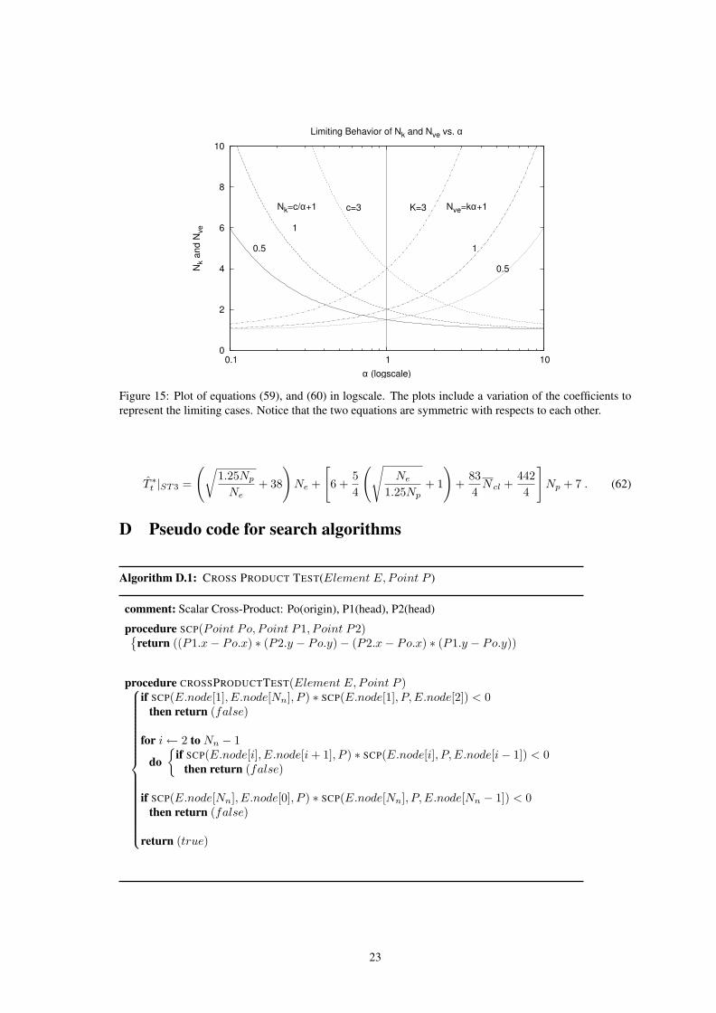
Figure 15: Plot of equations (59), and (60) in logscale. The plots include a variation of the coefficients torepresent the limiting cases. Notice that the two equations are symmetric with respects to each other.

T ∗t |ST3 =

(√1.25Np

Ne+ 38

)Ne +

[6 +

54

(√Ne

1.25Np+ 1

)+

834

N cl +4424

]Np + 7 . (62)

D Pseudo code for search algorithms

Algorithm D.1: CROSS PRODUCT TEST(Element E, Point P )

comment: Scalar Cross-Product: Po(origin), P1(head), P2(head)

procedure SCP(Point Po, Point P1, Point P2){return ((P1.x− Po.x) ∗ (P2.y − Po.y)− (P2.x− Po.x) ∗ (P1.y − Po.y))

procedure CROSSPRODUCTTEST(Element E, Point P )

if SCP(E.node[1], E.node[Nn], P ) ∗ SCP(E.node[1], P, E.node[2]) < 0then return (false)

for i← 2 to Nn − 1

do{

if SCP(E.node[i], E.node[i + 1], P ) ∗ SCP(E.node[i], P, E.node[i− 1]) < 0then return (false)

if SCP(E.node[Nn], E.node[0], P ) ∗ SCP(E.node[Nn], P, E.node[Nn − 1]) < 0then return (false)

return (true)

23

Algorithm D.2: INITIALIZEBOUNDINGBOX(Element E)

comment: 4 Assignment Operations

E.xmin = E.node[0].xE.xmax = E.node[0].xE.ymin = E.node[0].yE.ymax = E.node[0].y

comment: 3× 4 Comparison + 6max or 2min Assignment Operations

for i← 1 to 3

do

if E.xmin > E.node[i].xthen E.xmin = E.node[i].x

if E.xmax < E.node[i].xthen E.xmax = E.node[i].x

if E.ymin > E.node[i].ythen E.ymin = E.node[i].y

if E.ymax < E.node[i].ythen E.ymax = E.node[i].y

Algorithm D.3: ISINSIDETHEBOUNDINGBOX(Element E, Point P )

if P.x > E.xmax

then return (false)else if P.y > E.ymax

then return (false)else if P.x < E.xmin

then return (false)else if P.y < E.ymin

then return (false)else return (true)

Algorithm D.4: GET VIRTUAL ELEMENT INDEX(Point P )

comment: (1 Subtraction + 1 Division + 1 Cast Operation) × Dimension

procedure GET INDEX(V ector P, i, j){i = FLOOR((P.x− x0)/dx)j = FLOOR((P.y − y0)/dy)

Algorithm D.5: INITIALIZE VIRTUAL MESH(Elements List Ve)

procedure INITIALIZE VIRTUAL MESH(Elements List Ve)SETUP VIRTUAL MESH GEOMETRY(Ve)for each Element E ∈ Ve

do{

INITIALIZEBOUNDINGBOX(E) #see D.2ADD FINITE ELEMENT TO VIRTUAL MESH(E)

24

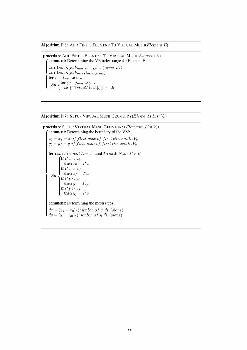
Algorithm D.6: ADD FINITE ELEMENT TO VIRTUAL MESH(Element E)

procedure ADD FINITE ELEMENT TO VIRTUAL MESH(Element E)

comment: Determining the VE index range for Element E

GET INDEX(E.Pmin, imin, jmin) #see D.4GET INDEX(E.Pmax, imax, jmax)for i← imin to imax

do{

for j ← jmin to jmax

do{V irtualMesh[i][j]← E

Algorithm D.7: SETUP VIRTUAL MESH GEOMETRY(Elements List Ve)

procedure SETUP VIRTUAL MESH GEOMETRY(Elements List Ve)

comment: Determining the boundary of the VM:

x0 = xf = x of first node of first element in Ve

y0 = yf = y of first node of first element in Ve

for each Element E ∈ V e and for each Node P ∈ E

do

if P.x < x0

then x0 = P.xif P.x > xf

then xf = P.xif P.y < y0

then y0 = P.yif P.y > yf

then yf = P.y

comment: Determining the mesh steps

dx = (xf − x0)/(number of x divisions)dy = (yf − y0)/(number of y divisions)

25