1

A CONSISTENT INTERPOLATION FUNCTION FOR THE SOLUTION OF RADIATIVE TRANSFER ON TRIANGULAR MESHES.

I – COMPREHENSIVE FORMULATION

Daniel R. ROUSSE,§, Fatmir ASLLANAJ Department of mechanical engineering, École de technologie supérieure, Canada

LEMTA, Nancy-Université, CNRS, France §Correspondence author. Fax: +1 514 396-8800, 7341. Email: Daniel.Rousse@etsmtl.ca

Abstract

This paper exhaustively presents a first-order skewed upwinding procedure for application to discretization numerical methods in the context of radiative transfer involving gray participating media. This scheme: (1) yields fast convergence of the algorithm; (2) inherently precludes the possibility of computing negative coefficients to the discretized algebraic equations; (3) reduces false scattering (diffusion); (4) is relatively insensitive to grid orientation; and (5) produces solutions completely free from undesirable oscillations. Theses attributes render the scheme attractive, especially in the context of combined modes of heat transfer and fluid flow problems for which computational time is a major concern. The suggested scheme has been validated by application to several basic test problems discussed in a companion paper.

Keywords: radiation, finite volume method, triangular meshes, participating media NOMENCLATURE O Centroid of an element p Control volume surface (panel)

φJ

Flux of φ (radiative) per unit solid angle, [W∙m-2∙sr-1] mnG Geometric quantity, [sr]

M Midpoints of element edges N Number of panels defining a control volume, Node of an element

φS Rate of volumetric generation of φ

IS Source of radiative intensity n Unit vector normal to a surface

wff ,, −+ Weighting functions Greek symbols φ Dependent variable Subscripts b Blackbody B Boundary n Control volume surface (panel) m Discrete direction l Element edge ϑ Integer function: nn =)(ϑ , n∀ = 1, 2, 3; and 3)( −= nnϑ , n∀ = 4, 5

2

P Node of reference r Radiation or Reference point Superscripts

m Discrete direction ′ Incoming direction → Vectorial quantity Other symbols: ASME, JHT 1999, 121(4), 770-773. 1. INTRODUCTION

One of the key issues of the numerical methods that solve the Radiative Transfer Equation (RTE) is the closure relation or spatial interpolation function for the discrete dependent variable intensity over the elements (or over control volumes) of the computational mesh [1]. This is then relevant for discrete ordinates methods (DOMs), finite volume methods (FVMs), control volume finite element methods (CVFEMs), and Finite Element Methods (FEMs).

Here the discussion pertains to such discretization methods and is not concerned with traditional zonal, Monte-Carlo, ray tracing, discrete transfer methods [2] or the more recently acknowledged collapsed dimension [3-5] and direct collocation meshless method [6,7].

A first interpolation scheme was introduced by Carlson and Lathrop [8] in the context of neutron transport problems: it is the diamond difference scheme. This scheme was the first to be implemented by Hyde and Truelove [9] and later by Fiveland [10] in their pioneering radiative heat transfer work. It has since been used extensively. However, as for the central difference scheme used in the context of convection-diffusion and fluid flow problems, the diamond scheme can produce negative coefficients (elemental negative intensities) in the discretized algebraic equations that approximate the original RTE. This procedure may lead to spatially oscillating, physically unrealistic distributions of the transported entity (intensity). Fix-up procedures have been proposed in attempts to solve this problem. All of them result in schemes that require more computational time per iteration than their original counterpart.

Decades later, Coelho and Aelenei [11] tested several high-order schemes, namely the MINMOD, CLAM, MUSCL, SMART schemes. They found that the use of high order schemes is only effective if the angular refinement yields low-angular discretization error as well. In this respect, the study of Cheng et al. [12] proposes a genuine method (called DRESDOR) that accounts for radiation in 6658 discrete directions in the hemispheric space to model the angular discretization appropriately.

Chai and co-workers [13], after testing several procedures, finally recommend to rely on the upwind scheme (US). In that paper, the upwind scheme (also called step scheme), the diamond scheme, the positive scheme proposed by Lathrop [14], and the positive intensity conditions suggested by Fiveland and Jessee [15] are discussed in the context of the discrete ordinates method. The paper also discusses the relative merits of variable weight schemes proposed by Jamaluddin and Smith [16] but indicates that, in general, schemes based on weighting factor less than unity could lead to physically unrealistic solutions. Liu et al. [17] showed that the criterion for an unconditionally stable scheme is that this weighting function

3

should be superior to 2⁄3. Berour and co-workers [18] propose a review of several of these differencing scheme efficiencies for the case of strong opacities in purely absorbing media.

One of the alternative recommended by Chai and co-workers [13], is to trace the downstream intensities at an integration point p to an upstream reference location r where the intensity can be computed or is known in terms of nodal values. This is the basis of the original CVFEM proposed by Rousse and Baliga [19] and Rousse [1, 20]. Although use of unidirectional upwinding removes the potential for spatial oscillations, such a procedure is burdened with excessive false diffusion (false scattering).

The smearing here is numerically (not physically) analogue to what is referred to as false diffusion in the context of fluid flow and convective heat transfer [21]. In this respect, numerical smearing can be referred to as false scattering, which is a numerical redistribution of energy rather than a physical phenomenon. Hence, the authors acknowledge the need for a scheme that models the skewness of radiative transport with improved accuracy. This has been done over a period of some ten years as exemplify by the papers of Chai et al. [13], Tan et al. [22], and Coelho [23].

In the paper of Jessee and Fiveland [24], the authors address the issue of spatial discretization in the context of numerical smearing. In that paper, the authors state that the upwind scheme is computationally inexpensive but first order accurate thus leading to poor modeling and numerical scattering, and that the diamond scheme modifications, required by the presence of negative coefficients, are not entirely satisfactory. To overcome these drawbacks, the authors investigated bounded high resolution schemes. They concluded that a bounded exponential or higher order scheme, with built-in flux limiters in which skewness is accounted for, would be promising. However, it could be mentioned that the non-linearity of the proposed high resolution schemes often necessitate an increase in computational time requirements. It is reported that these high resolution schemes may be competitive with the standard upwind scheme but for significantly scattering media or reflective boundaries and when the problem may allow the analyst to neglect other heat transfer modes.

Liu et al. [17] came to similar conclusions in their analyses of the conventional difference schemes and the SMART scheme. However, the authors recommend the use of the central difference scheme although this scheme may produce spurious oscillations, because it yielded integral quantities (flux, incident radiant energy) almost as accurate as the SMART scheme.

The avenue taken here is somewhat different; instead of using a high order scheme, a first order skew upwind scheme is proposed. It will be shown that the proposed scheme could be viewed as a skewed upwind scheme that ensures positive coefficient to the discretized algebraic equations while limiting the connectivity to a single finite element.

In the context of convection-diffusion and fluid flow problems, false diffusion can be substantially reduced through the use of a skewed upwind scheme such as that proposed by Raithby [25]. However, this procedure has the potential for developing spatial oscillations in the solution through the computation of negative coefficients in the discretized equations. Leonard [26], proposed a quadratic upstream interpolation scheme that considerably reduces the problem. However, his scheme does not entirely circumvent the calculation of negative coefficients.

4

Hassan et al. [27] proposed a procedure that solves the problem by restricting the range of the upstream weighting factor such that the influence coefficients cannot become negative. In some sense, this procedure based on a mathematical restriction on the upstream weighting factor, is akin to a similar ideas developed for the intensity of radiation calculation with the diamond scheme [14].

Conventional Galerkin finite element methods for convection-diffusion problems experience similar difficulties [28] and although several upwind type schemes have been suggested [29-32], they all more or less suffer from false diffusion.

Clearly, in the context of convective transport, a broad range of numerical procedures were proposed in attempts to reduce false diffusion and/or eliminate the negative coefficients problem. Among these, the skewed positive influence coefficient upwinding procedure proposed by Schneider and Raw [33], modified by Saabas [34], and by Rousse [20], was found to hold the premise of a suitable interpolation function for radiation intensity in the context of problems involving radiative heat transfer in participating media.

The present paper is concerned with the progressive development of an interpolation function for radiative intensity that does account for the directionality of the radiant energy propagation through a skewed approach, while simultaneously precluding the possibility of negative coefficients.

2. CVFEM FORMULATION

The solution of the radiative transfer equation (RTE) by a CVFEM requires the discretizations of both spatial and angular domains. The angular discretization of the RTE, which is solved along M discrete directions, leads to the solution of M sets of algebraic discretization equations [1].

2.1. Radiative transfer equation

For the sake of completeness, the multidimensional propagation of radiation in gray-diffuse enclosures filled with gray participating media is recalled here; it can be described by the following equation:

( ) ),(),(),( Ω+Ω−=ΩΩ⋅∇

sSsIsI Iβ (1)

where IS , the source function for radiant intensity, is given by:

∫ ′ΩΩ′ΦΩ′+Ω=Ωπ

ωπσκ

4

),(),(4

),(),( dsIsIsS bI

(2)

and the radiative boundary condition at a point B on a gray-diffuse surface is:

5

∫<⋅Ω′

′Ω′⋅Ω′−

+=Ω0)(

)()1()()(B

B

nBB

BBbBB dInTII

ωπε

ε (3)

In the formulation of CVFEMs, it is convenient to cast the governing partial differential equations in the following general form [21]:

φφ SJ =⋅∇

(4)

where φ stands for a general variable, φS is a volumetric generation rate or source term, and φJ

is the flux of φ . Eq. (1) may be readily obtained from this general equation by using:

),( ΩΩ=

sIJφ and ),(),( Ω+Ω−=

sSsIS Iβφ .

2.2. Domain discretization

In CVFEMs, the calculation domain is first spatially divided into elements. In a second step of discretization, each element is divided into sub-control volumes in such a manner that upon assembly of elements, complete control-volumes are formed around each node of the computational mesh. In two-dimensional and three-dimensional formulations, three-nodes triangular and four-nodes tetrahedral elements are used, respectively.

With regards to angular discretization, discrete ordinates-type or azimuthal discretizations can be used. Discretization details are provided elsewhere [1].

It should be noted that FVMs and FEMs do also need spatial and directional discretizations.

2.3. CVFEM approximation

An integral conservation equation corresponding to the RTE is obtained by applying the conservation principle to control volumes, V, and solid angles, mω , such that :

∫ ∫∫ ∫ =⋅mm VA

ddVSddAnJω

φω

φ ωω

(5)

where A is the surface area of the control volume, and n is a unit outward-pointing normal to the differential area element dA.

In the suggested CVFEM, the radiative properties and the scattering phase function are nodal values and are assumed to prevail over the control volume associated with this point and over a discrete solid angle mω , while the source term φS is linearized [21] and assumed constant over control volumes and solid angles. The radiant heat flux is assumed constant (average values are assumed) over control volume surfaces and solid angles [1].

6

The discretized integral conservation equation, corresponding to Eq. (5), in the direction mΩ

for a control volume associated with node P and having N control volume faces is finally:

mPmImP

mPP

N

nn

mn

mp VSVIAGI

Pnωωβ +−=∑

=1

(6)

where mpn

I is the radiative intensity evaluated on np along mΩ

; mnG is a geometrical quantity

defined below, eq.(7); nA is the surface area of a control volume surface np ; mPI is the radiative

intensity evaluated at node P along mΩ

; mIP

S is the value of the source term evaluated at node P

in direction mΩ

; PV is the volume surrounding node P; and mω is the solid angle associated with

direction mΩ

, respectively

The geometric function mnG is evaluated such that:

∫ ⋅Ω=m

dnG nmn

ω

ω

(7)

where nn is the unit outward-pointing normal to a panel np . The rationale behind these choices is discussed in [1].

To complete the CVFEM formulation, a relation between the value of the radiative intensity at control volume surfaces and that of this same quantity at the grid nodes of the finite element mesh is required. This relation is established by the prescription of an appropriate spatial interpolation function for intensities over the elements and this is the subject matter of the next section.

The issues of discretization equations, boundary conditions, and solution procedure are presented elsewhere [1] and are not repeated here to avoid this paper to become overly lengthy. 3. SKEW UPWINDING SCHEME

The nature of the discretized RTE does suggest that it is indeed highly desirable not only to account for radiative intensity at upstream locations when closure is needed, but also to reflect the direction of propagation of radiation. Here, attention is limited to those two features without regard to attenuation by absorption and out-scattering or reinforcement by emission and in-scattering in the interpolation functions.

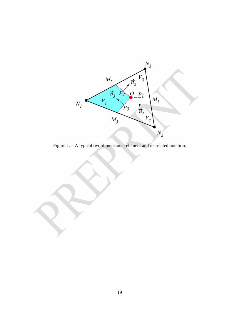
The convention adopted here is that depicted in Fig. 1. Careful study of this figure should help the reader in the following sections of the paper. Discussions are limited to the two-dimensional context for simplicity and clarity, but are very exhaustive to help the reader in implementing these ideas, if need be.

With reference to Figure 1, N1, N2, N3 denote the nodes of the finite element considered, O is the centroid of the element where a local Cartesian coordinate system will be translated, V1, V2, V3 are

7

partial control-volumes that will constitute the complete and non overlapping discretized volume of the calculation domain upon assembly of all triangular elements; p1, p2, p3 are the sub-control volume surfaces, n are the unit outward-pointing normal to the sub-control volume surfaces, and M are the mid-point, between two nodes, along the edge of a triangular element side. It is worth noting, for further reference, that M1 is opposite to N1 and similarly for the other two pair of nodes and midpoints.

3.1 An exponential scheme (ES)

The first scheme that was considered for implementation within the CVFEM was the

exponential scheme (ES) [1]. This scheme, based on a particular one dimensional solution of the RTE within an element, yielded very satisfactory predictions [19, 35]. However, this scheme suffers two major drawbacks: (1) it requires fix-up procedures to avoid computations of negative coefficients, and (2) exponentials are relatively expensive to compute. Hence, in the context of the development of comprehensive numerical methods for the solution of multiphase turbulent reacting flow combined with radiative heat transfer, such a scheme could lead to unacceptable computational time requirements. 3.2 An upwind scheme (US)

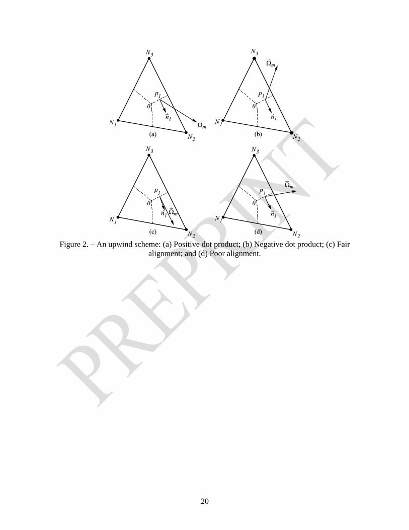
With the reference to Fig. 2, the implementation of this scheme is rather simple. If the dot product

1pm n

⋅Ω is positive (Fig. 2(a)), the value of the radiative intensity at the integration point

1p is that of the node located immediately counter clockwise with respect to the centroid, O, here node 3N .

On the other hand, if this dot product is negative (Fig. 2(b)), the value of radiative intensity at the integration point 1p is that of node 2N .

For any of the three control volume surfaces (panels), 1p , 2p , 3p , the implementation is straight-forward:

mN

mn

mN

mn

mp nnn

IwIwI)1()2(

)1(++

−+=ϑϑ

(8)

where the weighting function nw is defined as :

≡ 0MAX ,

GG

wmn

mnm

n (9)

and the integer function )(nϑ is such that nn =)(ϑ , n∀ = 1, 2, 3; and 3)( −= nnϑ , n∀ = 4, 5. The weighting functions, m

nw , for each element, can be evaluated prior to the iterative procedure as they are geometric quantities independent of the radiation transfer problem.

8

The upwind scheme (US) is simple and yields rapid convergence of the solution procedure. Moreover, it ensures that no negative coefficients are produced in the discretization equations. However, it is obvious that for several discrete directions, the directionality of radiant propagation is not very accurately taken into account. For discrete directions where the node of influence, 3N , is in a more or less direct line of sight when observed from the integration point

1p , such as in Fig. 2(c), the predictions of intensity along that direction will be good. However, for the situation depicted in Fig. 2(d), severe false scattering (numerical smearing) will occur and for that direction the predictions of radiant intensity will be far less accurate. Moreover, it is clear that this scheme will produce solutions that are very sensitive to the shape of elements. Nevertheless, the upwind scheme was retained as an alternative because it is the simplest and therefore cheapest scheme and the inaccuracies it involves are averaged over all directions when the radiative fluxes or radiant incident energy are evaluated. Hence, the results for the radiative fluxes and radiant incident energy were found to be in fair agreement with those obtained with higher order schemes.

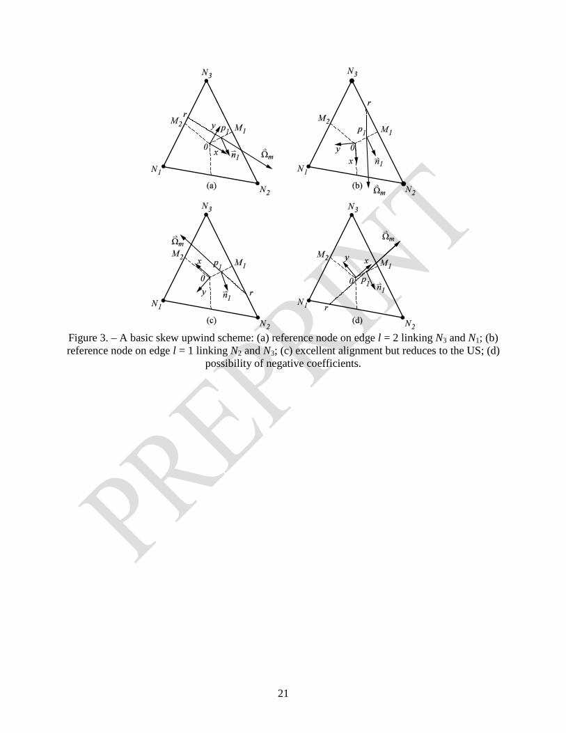
3.3 A basic skew upwind scheme (BSUS)

With reference to Fig. 3, the basic skew upwind scheme (BSUS), applied to the triangular element discretized into three equal sub-control volumes, determined the value of the intensity at the integration point, 1p , by tracking back along the projection of a discrete direction, mΩ

, from

1p until the pencil (path) of radiation intersects the element edge at a reference point, r. Here, the notation assumes that the edge number, l, is that of its corresponding midpoint, M. This notation is used for the ease of presentation and implementation.

The value taken for the radiative intensity at position r is then based on an interpolated value, along this element edge, of the corresponding nodal values (for example, nodes 2N and 3N in Fig. 3(b)). In the context of upwinding (no attenuation), m

rmp nn

II = . This leads to a value of the intensity at the integration point that is an average of two nodal values.

When 11 =mw , see Eq. (9), the reference point will lie either along edge 2=l or 1=l . In Fig. 3(a), with respect to a local Cartesian coordinate system located at the centroid of the element, O, that is oriented so as to have its axis x aligned with the projection of mΩ

in the plane of the problem, the reference point, r, lies on the edge 2=l for which:

113 NpN yyy ≥≥ . In Fig. 3(b), the reference point, r, lies on the edge 1=l for which:

312 NpN yyy ≥≥ . In any of these two

cases, mpI

1 can be expressed as a linear function of the intensity at two nodes such that:

mNl

mNl

mp ll

IfIfI)2()1(1

)1( 11 ++−+=

ϑϑ (10)

where the weighting function lf1 in terms of the local and aligned coordinate directions is :

9

)2()1(

)2(1

1++

+

−

−=

ll

l

NN

Npl yy

yyf

ϑϑ

ϑ (11)

and l is either 1 or 2 according to the relative y-coordinate of node 3N with respect to 1p .

Similarly, when 01 =mw , the reference point will lie either along edge 3=l or 1=l . In Fig. 3(c), the reference point, r, lies on the edge 1=l for which:

312 NpN yyy ≥≥ , and the above expression apply. It can readily be observed that the equations are also valid for the case shown in Fig. 3(d) for which:

211 NpN yyy ≥≥ . Here, the relative y-coordinate of node 2N with respect to 1p determines whether 3=l or 1=l .

Generalizing the former expressions, for any of the three control volume surfaces, 1p , 2p , 3p , yields:

mNnl

mNnl

mp lln

IfIfI)2()1(

)1(++

−+=ϑϑ

(12)

where the expression of nlf is :

)2()1(

)2(

++

+

−

−=

ll

ln

NN

Npnl yy

yyf

ϑϑ

ϑ (13)

However, this strategy can be challenged for several reasons : (1) for a given direction, when both nodes are located upstream with respect to the integration point 1p , such as nodes N1 and N3 in Fig. 3(a), there is no guarantee that the intensity at reference point, r, will physically be a linear interpolation of the nodal values. Except, in a highly scattering media or when a fine spatial discretization is used; (2) for a particular direction, a node N could be located downstream with respect to the integration point such as node N2 in Fig. 3(b) where 2N is found to have an influence on m

pI1. This could lead to negative coefficients in the discretized algebraic equations;

(3) for some very limited cases only, such as that shown in Fig. 3(c), the scheme would propose a fair representation of the physics (without attenuation). But in this case, it reduces to the US; and (4) for the case represented in Fig. 3(d), the dependence on the intensity at node 1N constitute an outflow of radiant energy from the control volume associated with node 2N . Thus if m

NI1

decreases, mNI

2 will increase proportionately. And this clearly shows that negative coefficients

could be calculated in the numerical solutions.

Remedies to avoid negative coefficients could be thought as follows: (1) when a node N is located downstream with respect to the integration point such as node N2 in Fig. 3(b), the weighting factor (here 11f ) could be set to zero (when the local x-coordinate difference between node N2 and point p1 is positive). Similarly, 111 =f when node 3N is located downstream of point 1p ; (2) to avoid the outflow problem illustrated in Fig. 3(d), the simplest remedy would be

10

to have an influence of 2N only. Clearly, this overrides the properties of the basic skew upwind scheme (BSUS) and reduces it more or less to the upwind scheme (US) but with more computational time requirement.

Nevertheless, having in mind its limitations, the second scheme retained for comparison is the basic skew upwind scheme (BSUS) described by Eq. (12).

3.4 An intermediate skew upwind scheme (ISUS)

To avoid having downstream influences and negative coefficients, an intermediate skew upwinding scheme (ISUS) is now introduced. In this scheme, that embeds ideas discussed in the previous subsection, the value of the intensity along the elements edges that link the nodes is assumed to be constant up to the midpoint of the edges: the value of intensity on the edges that delimit sub-control nV is m

NnI .

With reference to Fig. 4(a), line M2 – a represents a line of discontinuity of the intensity originating from the volumes associated with 1N and 3N . The relative influence of both nodes on the value of the radiative intensity at 1p is then a weighted average of m

NI3 and m

NI1, the

weights being the ratio bcbM −−2 and bccM −−2 , respectively. On panel 1p , mNI

1

prevails from the centroid, O, to point a, then mNI

3 prevails from a to 1M . Segment bc − is the

projection, normal to mΩ

, of the control volume surface 1p over edge l = 2.

When 11 =mw (see Eq. (9)), with respect to coordinate axes located at the centroid, O, and oriented such that the x-axis is aligned with the two-dimensional projection of mΩ

, 1My is

positive and as long as 02≤My the node of influence for 1p will be 3N only. The case for which

02=My is shown in Fig. 4(b). When the situation depicted in Fig. 4(a) prevails,

mN

mN

mp IfIfI

311)1( 11

++ −+= (14)

where 121 MM yyf =+ . When

12 MM yy ≥ , the node of influence for 1p will be 1N only. Fig. 4(c) depicts the situation for which

12 MM yy = .

To account for the above-described three possibilities, Eq. (14) will be valid if the weighting function is defined such that

≡+ 1,0,MAXMIN

1

21

M

M

yy

f (15)

11

When 01 =mw , as long as 03≥My the node of influence for 1p will be 2N only. When the

situation depicted in Fig. 4(d) occurs,

mN

mN

mp IfIfI

211)1( 11

−− −+= (16)

where 131 MM yyf =− . When

13 MM yy ≤ , the node of influence for 1p will be 1N only. Hence, with the following weighting function

≡− 1,0,MAXMIN

1

31

M

M

yy

f (17)

Eq. (16) provides the value of mpI

1 for the three geometric possibilities with 01 =w .

Although the expressions for f are mathematical expressions evaluated through the determination of the local y-coordinate of the element edges midpoints, the resulting expressions have a direct physical interpretation. For example, with respect to the element depicted in Fig. 4(a), it can be seen that +

1f is the ratio of the radiative flux that crosses control surface 2MO − into direction

mΩ

over the radiative flux that crosses control surface 1MO − along the same direction when there is no attenuation or reinforcement within the element. Specifically,

1

2

1

21

MO

MO

M

M

qq

yy

f−

−+ =≡

(18)

From this expression it can be concluded that the weighting factor will be equal to this ratio as long as the medium in the element, for the purpose of interpolation only, is assumed to be transparent.

Considering mw1 as defined in Eq. (9), it is possible to account for the negative or positive value of

1pm n

⋅Ω by expressing mpI

1 as

])1()[1(])1([21311 111111

mN

mN

mmN

mN

mmp IfIfwIfIfwI −−++ −+−+−+= (19)

Finally, with the use of the integer function )(nϑ defined previously, a general mathematical expression of m

pnI at any of the three panels, 1p , 2p , 3p , can be arrived at :

])1()[1(])1([)1()2(

mN

mn

mN

mn

mn

mN

mn

mN

mn

mn

mp nnnmn

IfIfwIfIfwI++

−−++ −+−+−+=ϑϑ

(20)

where

12

≡

≡ ++ −+ 1,0,MAXMIN;1,0,MAXMIN )1()2(

n

n

n

n

M

Mmn

M

Mmn y

yf

y

yf ϑϑ (21)

with n = 1, 2, 3 for panels 321 ,, ppp , respectively. The superscript m is added to the definition of the weighting function f to permit calculation of these functions prior to the iterative solution process.

In Fig. 4(a), the contribution of 1N is still seen by the equations for panel 1p (between the centroid O and point a), but this contribution has no effect on the radiant energy conservation balance for the control volume associated with 3N after the contribution of 2p is accounted for. Because without attenuation m

pI2 is m

NI1, all influence of 1N on 1p , for this case, cancel. This is

valid as long as there is no attenuation involved, at the interpolation level, along the propagation path within an element. Otherwise, a net flux of radiant energy is still possible. That is, if the flux entering 2p is different from that entering 1p , between O and a, negative coefficients would still be possible.

The value of the intensity at 1p in Fig. 4(a) is simply a weighted average of that at node 1N and

3N . On panel 1p , mNI

1 prevails from the centroid to point a, then, from a to 1M , m

NI3 prevails.

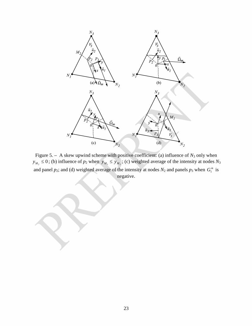
3.5 A Skew Upwinding Scheme (SUS)

The ideas embedded in the skew positive coefficient upwind scheme (SUS), which

involve a flux-weighted average of the intensity over control volume faces, are first outlined for control volume surface 1p depicted in Fig. 5(a). It has been seen that as long as there is no attenuation within the elements, the ISUS should improve accuracy over the US and avoid negative coefficients in the discretized algebraic equations. However, in a further refinement of the proposed scheme, it could be desirable to account for attenuation within the element. In this section, for a positive value of the radiant heat flux at 1p (see Fig. 5(a)), that is when 11 =mw , it is then mostly desirable to express the value of intensity at 1p directly in terms of that at 2p and that at node 3N such that

mN

mmp

mmp IfIfI

321)1( 11

++ −+= (22)

with +mf1 being defined appropriately.

This modification of the ISUS involves that: (1) negative coefficients can not be computed, since throughputs of radiant energy are correctly accommodated irrespective of the function +mf1 , and (2) a simultaneous set of equations involving the three integration point intensities (that is at p1, p2, and p3) must be solved to determine these values in terms of the nodal values. To generalize this SPCUS, a similar definition of +mf1 to that used in Eq. (21) is employed with the obvious restriction that 10 ≤≤ f .

13

To ensure a positive contribution to the coefficients when the radiative flux at 2p is negative – coming out of sub-control volume 3V in Fig. 5(a) – we need that m

Nmp II

31= : the values of m

pI1 and

mpI

2 at the panels 1p and 2p for this situation should only depend on the value of mI at node 3,

which is located upstream of these two surfaces: this implies that 01 =+mf in Eq. (22). On the other hand, if mG2 is positive – coming into sub-control volume 3 in Fig. 5(b) – and greater than

mG1 , only mpI

2 should influence the value of m

pI1, because the amount of energy transported by

radiation out of control volume 3V across panel 1p has to be greater than or equal to what comes in by radiation through panel 2p , in order to ensure the positiveness of coefficients [1, 27, 34]. For this case +mf1 = 1. In other situations, such as in Fig. 5(c), the function +mf1 is just the ratio of the directional integral of pn

⋅Ω over mω for control surface 2p to that over 1p .

Consequently, a general expression for +mf1 , for a positive mG1 can be defined as

≡+ 1,0,MAXMIN

1

21 m

mm

GGf (23)

The subscript 1 stipulates the association with panel 1 and the superscript + indicates that mG1 is positive.

If these same guide lines are followed when radiation is crossing control volume surface 1p in the negative direction such as in Fig. 5(d) – mG1 is negative – then an equation, involving node 2 and panel 3p , can readily be obtained such that

mN

mmp

mmp IfIfI

231)1( 11

−− −+= (24)

where −mf1 is defined as

≡− 1,0,MAXMIN

1

31 m

mm

GG

f (25)

Introducing the weighting function, mw1 , defined as in Eq. (9), it is possible to account for the negative or positive value of the radiative flux at 1p by expressing m

pI1 as

])1()[1(])1([23321 111111

mN

mmp

mmmN

mmp

mmmp IfIfwIfIfwI −−++ −+−+−+= (26)

Finally, with the use of the integer function )(nϑ defined previously, a general mathematical expression of m

pnI at any of the three panels, 321 ,, ppp , can be arrived at:

])1()[1(])1([)1()2()2()1(

mN

mn

mp

mn

mn

mN

mn

mp

mn

mn

mp nnnnn

IfIfwIfIfwI++++

−−++ −+−+−+=ϑϑϑϑ

(27)

14

where

≡

≡ +−++ 1,0,MAXMIN;1,0,MAXMIN )2()1(

mn

mnm

nmn

mnm

n GG

fG

Gf ϑϑ (28)

with n = 1, 2, 3 for panels 321 ,, ppp , respectively.

4. CONCLUDING REMARKS

This paper presents the detailed derivation of a skew, positive coefficient, upwind scheme for the computation of radiative transport in enclosures discretized by use of triangular meshes. The exhaustive description was intended for the analyst who may want to implement such a procedure in his or her own numerical method. From the proposed descriptions, ideas could easily be extrapolated for the analyst who may want to implement these ideas on rectangular meshes

The proposed scheme is based on the application of sound physical arguments, resulting in: (1) fast convergence of the algorithm; (2) inherent preclusion of the possibility of computing negative coefficients to the discretized algebraic equations; (3) relatively low levels of false scattering; (4) relative insensitivity to grid orientation; and (5) solutions completely free from undesirable oscillations. These attributes render the scheme attractive, especially in the context of combined modes of heat transfer and fluid flow for which computational time is a major concern. The performances of the proposed scheme are readily available in a companion paper [36].

The development presented in this paper, considers pure upwinding, that is the effect of intensity attenuation and reinforcement are not considered within an element. In this way, the specific features avoiding negative coefficients are readily appreciated. One of the interesting features of the proposed scheme is that it can be used in the context of combined modes heat transfer and fluid flow problems employing the same procedure for the solution of the algebraic discretized conservation equations. Therefore, although implemented in the context of a CVFEM, the ideas are readily amenable for incorporation in a FVM or a FEM.

APPENDIX A: Closures relations

Eqs. (8), (12), (20), and (27) are systems of equations for the unknowns mpI . These

systems of equations can conveniently be written in a matrix form, yielding [ ] [ ] 13331333 ×××× = m

Nmp IBIA (29)

or

15

=

mN

mN

mN

mp

mp

mp

III

bbbbbbbbb

III

aaaaaaaaa

3

2

1

3

2

1

333231

232221

131211

333231

232221

131211

(30)

A.1 Upwind scheme

For a two-dimensional implementation of the upwind scheme (US), the A matrix is the identity matrix while the coefficients of the B matrix are:

mjjj

mjjjjj wbwbb =−== ++ )2()1( );1(;0 ϑϑ (31)

A.2 Basic skew upwind scheme

To implement the basic skew upwind scheme in two-dimensions, the A matrix is also the identity and matrix B can be constructed such that, when )1( +≥≥ jNpN yyy

ij ϑ , we obtain :

0);1(; )2()1( =−== ++ jiijjiijij bfbfb ϑϑ (32) A.3 Intermediate skew upwind scheme

In this case, the A matrix is once again the identity matrix and matrix B can be constructed such that:

)1();1)(1(;)1( )2()1(+

+−

+−+ −=−−=−+= m

jmjjj

mj

mjjj

mj

mj

mj

mjjj fwbfwbfwfwb ϑϑ (33)

The full matrix coefficients for the ISUS are :

)1()1()1)(1()1)(1()1()1(

)1()1)(1()1(

33333333

22222222

11111111

−+−−−−−−+−

−−−−+

−++−

−−++

+−−+

mmmmmmmm

mmmmmmmm

mmmmmmmm

fwfwfwfwfwfwfwfw

fwfwfwfw

A.4 Skew positive coefficient upwind scheme

For the implementation of the SPCUS, the coefficients of matrices A and B are

)1();1)(1(;1

)1(;;1

)2()1(

)2()1(

++

−+

−+

++

−=−−==

−−=−==mj

mjjj

mj

mjjjjj

mj

mjjj

mj

mjjjjj

fwbfwbb

fwafwaa

ϑϑ

ϑϑ (34)

The matrix coefficients for the SPCU scheme are :

1)1(1)1(

)1(1

3333

2222

1111

−−−−−−−−−

−+

+−

−+

fwfwfwfw

fwfw

0)1()1)(1()1)(1(0)1(

)1()1)(1(0

3333

2222

1111

−−−−−−

−−−

+−

−+

+−

fwfwfwfw

fwfw

16

These matrices involve geometric quantities only. They can be computed before the iterative solution procedure that solves for intensity begins. Acknowledgements – The authors gratefully acknowledge Rodolphe Vaillon (CNRS researcher, CETHIL, INSA de Lyon), Guillaume Gautier (Eng, PSA Group), and Mathieu Francoeur (Researcher, University of Kentucky) for their participation, collaboration and/or comments during these research works. The authors are also grateful to the Natural Sciences and Engineering Research Council of Canada (NSERC). Thanks go to Alan Wright for helping in the preparation of this manuscript. REFERENCES 1. D. R. Rousse, Numerical Predictions of Two-Dimensional Conduction, Convection, and

Radiation Heat Transfer. I – Formulation, Int. J. Thermal Sciences, vol. 39 (3), pp. 315-331, 2000.

2. V. Feldheim, and P. Lybaert, Solution of Radiative Heat Transfer Problems with the Discrete Transfer Method Applied to Triangular Meshes, J. Comput. Appl. Math., vol. 68, pp. 179–190, 2004.

3. P. Mahanta, and S. C. Mishra, Collapsed dimension method applied to radiative transfer problems in complex enclosures with participating medium, Num. Heat Transfer B, vol. 42 (4), pp. 367-388, 2002.

4. S. C. Mishra, P. Talukdar, D. Trimis, and F. Durst, Computational efficiency improvements of the radiative transfer problems with or without conduction - a comparison of the collapsed dimension method and the discrete transfer method, Int. J. Heat Mass Transfer, vol. 46 (16), pp. 3083-3095, 2003.

5. S. C. Mishra, N. Kaur, and H.K. Roy, The DOM approach to the collapsed dimension method for solving radiative transport problems with participating media, Int. J. Heat Mass Transfer, vol. 49 (1-2), pp. 30-41, 2006.

6. J. M. Zhao, and L. H. Liu, Second-order radiative transfer equation and its properties of numerical solution using the finite-element method, Num. Heat Transfer B, vol. 51, pp. 391–409, 2007.

7. J. Y. Tan, J. M. Zhao, L. H. Liu, and Y. Y. Wang, Comparative study on accuracy and solution cost of the first/second-order radiative transfer equations using the meshless method, Num. Heat Transfer B, vol. 55, pp. 324-337, 2009.

8. B. G. Carlson, and K. D. Lathrop, Transport Theory – The method of Discrete-Ordinates, In Computing Methods in Reactor Physics, Gordon and Breach, New York, 1968.

9. D. J. Hyde, and J. S. Truelove, The Discrete Ordinates Approximations for Multidimensional Radiant Heat Transfer in Furnaces, Technical Report, UKAEA, Report number AERE-R8502, 1976.

10. W. A. Fiveland, Discrete-Ordinates Solutions of the Radiative Transport Equation for Rectangular Enclosures, ASME J. Heat Transfer, vol. 106 (2), pp. 699-706, 1984.

11. P. J. Coelho, and D. Aelenei, Application of high-order spatial resolution schemes to the hybrid finite volume/finite element method for radiative transfer in participating media, Int. J. Numer. Method Heat Fluid Flow, vol. 18 (2), pp.173–184, 2008.

12. Q. Cheng, H. C. Zhou, Y. L. Yu, and D. X. Huang, Highly-directional radiative intensity in a 2-D rectangular enclosure calculated by the DRESOR method, Num. Heat Transfer B, vol. 54 (4), pp. 354-367, 2008.

17

13. J. C. Chai, S. V. Patankar, and H. S. Lee, Evaluation of Spatial Differencing Practices for the Discrete-Ordinates Method, J. Thermophys Heat Transfer, vol. 8 (1), pp. 140-144, 1994.

14. K. D. Lathrop, Spatial Differencing of the Transport Equation: Positivity vs Accuracy, J. Comp. Physics, vol. 4, pp. 475-498, 1969.

15. W. A. Fiveland, and J. P. Jessee, Comparisons of Discrete Ordinates Formulations for Radiative Heat Transfer in Multidimensional Geometries, J. Thermophys Heat Transfer, vol. 9, pp. 47-54, 1995.

16. A. S. Jamaluddin, and P. J. Smith, Predicting Radiative Transfer in rectangular Enclosures using the Discrete Ordinates Method, Combust. Sci. Tech, vol. 59, pp. 321-340, 1988.

17. F. Liu, H. A. Becker, and A. Pollard, Spatial Differencing Schemes of the Discrete-Ordinates Method, Num. Heat Transfer B, vol. 30, pp. 23-43, 1996.

18. N. Berour, D. Lacroix, and G. Jeandel, Radiative and conductive heat exchanges in high temperature glass melt with the Finite Volume Method approach. Influence of several spatial differencing schemes on RTE solution, Num. Heat Transfer A, vol. 49, pp. 567-588, 2006.

19. D. R. Rousse, and R. B. Baliga, Formulation of a Control-Volumes Finite Element Method for Radiative Transfer in Participating Media, In Proc. 7th Int. Conf. Num. Meth. Thermal Problems, pp. 786-795, Stanford, 1991.

20. D. R. Rousse, Numerical Predictions of Multidimensional Conduction, Convection and Radiation Heat Transfer in Participating Media, Ph.D. thesis, McGill University, Montréal, 1994.

21. S. V. Patankar, Numerical Heat Transfer and Fluid Flow, Hemisphere, Washington, 1980. 22. H. P. Tan, H. C. Zhang, and B. Zhen, Estimation of Ray Effect and False Scattering in

Approximate Solution Method for Thermal Radiative Transfer Equation, Numer. Heat Transfer A, vol. 46, pp. 807–829, 2004.

23. P. J. Coelho, The role of ray effects and false scattering on the accuracy of the standard and modified discrete ordinates methods, J. Quant. Spectrosc. Radiat. Transfer, vol. 73 (2-5), pp. 231–238, 2002.

24. J. P. Jessee, and W. A. Fiveland, Bounded, High-Resolution Differencing Schemes Applied to the Discrete Ordinates Method, J. Thermophys. Heat Transfer, vol. 11, pp. 540-548, 1997.

25. G. D. Raithby, Skew Upstream differencing Schemes for Problems Involving Fluid Flow, Comp. Meth. In App. Mech. and Eng., vol. 9, pp. 153-164, 1976.

26. B. P. Leonard, A Stable and Accurate Convective Modelling Procedure Based on Quadratic Upstream Interpolation, Comp. Meth. In App. Mech. and Eng., vol. 19, pp. 59-98, 1979.

27. Y. A. Hassan, J. G. Rice, and J. H. Kim, A Stable Mass-Flow-Weighted Two-Dimensional Skew Upwind Scheme, Num. Heat Transfer, vol. 6, pp. 395-408, 1983.

28. P. M. Gresho, and R. L. Lee, Don’t Suppress the Wiggles – They’re Telling you Something!, In Proc. Symposium Finite Element Methods for Convection Dominated Flows, pp. 37-61, ASME Winter Ann. Meeting, New York, 1979.

29. I. Christie, D. F. Griffiths, A. R. Mitchell, and O. C. Zienkiewicz, Finite Element Methods for Second Order Differential Equations with Significant First Derivatives, Int. J. Numer. Methods Eng., vol. 10, pp. 1389-1396, 1976.

30. J. C. Heinrich, P. S. Huyakorn, O. C. Zienkiewicz, and A. R. Mitchell, An Upwind Finite Element Method Scheme for Two-Dimensional Convective Transport Equations, Int. J. Numer. Methods Eng., vol. 11, pp. 131-143, 1977.

18

31. P. S. Huyakorn, Solution of Steady-State Transp Element Scheme, Appl. Math, Modelling, vol. 1, pp. 187-195, 1977.

32. T. J. R. Hughes, W. K. Liu, and A. N. Brooks, Finite Element Analysis of Incompressible Viscous Flows by the Penalty Function Formulation, J. Comp. Phys., vol. 30, pp. 1-60, 1979.

33. G. E. Schneider, and M. J. Raw, A Skewed Positive Influence Coefficient Upwinding Procedure for Control Volume Based Finite Element Convection Diffusion Computation, Num. Heat Transfer, vol. 9, pp. 1-26, 1986.

34. H. J. Saabas, A CVFEM for three-Dimensional, Incompressible, Viscous Fluid Flow, Ph.D. thesis, McGill University, Montréal, 1991.

35. D. R. Rousse, G. Gautier, J. F. and Sacadura, Numerical Predictions of Two-Dimensional Conduction, Convection, and Radiation Heat Transfer. II – Validation, Int. J. Thermal Sciences, vol. 39 (3), pp. 332-353, 2000.

36. D. R. Rousse, F. Asllanaj, N. Ben Salah, and S. Lassue, A consistent interpolation function for the solution of radiative transfer on triangular meshes. II – Validation, Num. Heat Transfer B, (accepted), 2010.

19

Figure 1. – A typical two-dimensional element and its related notation.

20

Figure 2. – An upwind scheme: (a) Positive dot product; (b) Negative dot product; (c) Fair

alignment; and (d) Poor alignment.

21

Figure 3. – A basic skew upwind scheme: (a) reference node on edge l = 2 linking N3 and N1; (b) reference node on edge l = 1 linking N2 and N3; (c) excellent alignment but reduces to the US; (d)

possibility of negative coefficients.

22

Figure 4. – An intermediate skew upwind scheme: (a) weighted average of the intensity at nodes N3 and N1; (b) influence of N1 only when

21 MM yy ≤ ; (c) influence of N3 only when 02≤My ; and

(d) possibility of negative coefficients.

23

Figure 5. – A skew upwind scheme with positive coefficient: (a) influence of N3 only when

02≤My ; (b) influence of p2 when

21 MM yy ≤ ; (c) weighted average of the intensity at nodes N3

and panel p2; and (d) weighted average of the intensity at nodes N2 and panels p3 when mG1 is negative.