arX

iv:a

dap-

org/

9710

001v

1 6

Oct

199

7

Evolution and extinction dynamics in rugged fitness

landscapes.

Paolo Sibani and Michael Brandt

Fysisk Institut

Odense Universitet,

Campusvej 55, DK5230 Odense M

Denmark

Preben Alstrøm

Niels Bohrs Institut

Københavns Universitet,

Blegdamvej 17, DK2100 København N

Denmark

October 29, 2018

Abstract

After an introductory section summarizing the paleontological data and someof their theoretical descriptions, we describe the ‘reset’ model and its (in partanalytically soluble) mean field version, which have been briefly introduced inLetters[1, 2]. Macroevolution is considered as a problem of stochastic dynamicsin a system with many competing agents. Evolutionary events (speciations andextinctions) are triggered by fitness records found by random exploration of theagents’ fitness landscapes. As a consequence, the average fitness in the system in-creases logarithmically with time, while the rate of extinction steadily decreases.This non-stationary dynamics is studied by numerical simulations and, in a sim-pler mean field version, analytically. We also consider the effect of externallyadded ‘mass’ extinctions. The predictions for various quantities of paleontologicalinterest (life-time distribution, distribution of event sizes and behavior of the rateof extinction) are robust and in good agreement with available data.

1 Introduction and background

Life on earth originated 3.5 billion years ago. According to the earliest record oflife, the first organisms were primitive one-celled non-photosynthesizing bacteria. Twobillion years then followed, before more complex multicelled organisms appeared ina catastrophic event called the Cambrian explosion. This evolutionary event, whichtook place about 600 million years ago, led to a diversity of new species, and to aremarkable fossil record for the following Phanerozoic period, which provides valuableand fundamental material for scientists who seek insight into the fascinating historyof life on earth.

Unfortunately, the fossil record is often limited when it comes to understanding thedevelopment of a given species at the level of organisms, i.e. the micro-evolutionary

1

processes. However, the record makes out a good statistical material at the macro-evolutionary level, where species and higher taxa are the basic units considered[3]. Atthis and higher taxonomical levels, evolutionary measures, as for instance the distri-bution of life spans, provide a good characterization of biological evolution and a basisfor understanding its underlying mechanism.

The evolution of species is typically sketched in the form of evolutionary trees withseveral lineage branchings. Whenever a lineage branches, it marks the appearance ofnew species (speciation), and whenever it stops, it marks the extinction of a species.We note that almost all species are extinct[4]. The possibility of hybridization, wheretwo lineages merge to form a new intermediate species, is normally not seen. Otherevolutionary changes are essential, the most prominent being the phyletic transfor-mations taking place along a lineage. These transformations are basically Darwinianchanges in species due to natural selection. The extinctions associated with phyletictransformations are called pseudo-extinctions.

Several questions arise when this Darwinian picture of evolution is taken undercloser scrutiny. Did species always have time to adapt to the changes in their envi-ronment? And what are the selection mechanisms ( if any ) that on a species leveldetermine who is to survive and who is to go extinct? Is evolution mostly characterizedby gradual changes, or is it rather characterized by ‘quantal jumps’ or ‘punctuations’,where new species are formed on a relatively short geological time scale?

We may further ask: can evolution be described by dynamical processes fluctuatingaround fix values, or is there a sense of direction in biological evolution, expressed, forexample, by a steadily increasing fitness measure? Why should nature select an averagelife time for species to be four million years? Why not four thousand years or 4 billionyears?

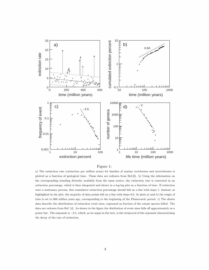
Explanations of evolutionary and extinction history can be coarsely classified ac-cording to their standing on the question of gradualism, to the importance they conferto ‘bad luck’ as opposed to ‘bad genes’[5], and finally according to their view on station-arity. All these issue have been intensely debated by paleontologist. From fossil data,it seems to us that nature has indeed not selected an equilibrium. For example, thestanding diversity of families of marine vertebrates[6] has increased by a large factorover the last 600 million years while, in the same period, the body plan complexity (the number of different somatic cells in the most complex of the taxa extant at a giventime ) has increased sixhundredfold[7]. The extinction rate does not appear to havereached an equilibrium either. Rather it seems to have a downward trend, as notedby Raup and Sepkoski[6] in 1982. Their data are reproduced in Fig. 1a. The decay ofextinction intensity can be highlighted by integrating the extinction rate, measured asa percent of standing diversity. The accumulated extinction rate percent describes thenumber of extinctions in a (hypothetical) system with a constant standing diversity. Ifevolutionary dynamics were a stationary process, with – on average – an equal numberof events taking place in any given time interval, this quantity would increase linearlyin time. Instead, as shown in Fig. 1b, it increases as a power law R(t) = t1−γ , and,correspondingly, the percentual rate of extinction r(t) decays as t−γ . The numericalvalue of γ is ≈ 0.4. Admittedly, the extinction record shows large fluctuations. Theevents which fall outside the expected statistical variation[8] are mainly related to thefive big mass extinctions, which have attracted enormous interest, presumably dueto their catastrophic impact on the ecosystem. The now most commonly acceptedexplanation of these events are meteor impacts[9].

2

Meteor craters have been looked for and identified to account not only for the massextinctions but also for several minor events, where a diversity of species seems to sud-denly disappear within a short geological time span. However, since mass extinctionsonly represent a small fraction of the data, they only exert a relatively minor influenceon the extinction rate.

An intriguing result of the decay of the extinction rate is its direct influence onother evolutionary measures. Consider for instance the frequency G(x) of extinctionevents in which a fraction x of the extant species are killed. The empirical form ofthis quantity is reproduced in Fig.1c after Raup’s data [4]. If p(x, t) is defined asthe joint probability density that an extinction of size x happens at time t, we thenhave G(x) ∝ ∫

p(x, t)dt and r(t) ∝ ∫

p(x, t)dx. Let us now for simplicity neglectfluctuations altogether, i.e. assume that extinctions of a given size only take placeat a given time, with the biggest extinction coming first. If a stage has length d,the fraction x0(t) of the system which is removed at time t is proportional to dr(t).Furthermore, one can easily show that our deterministic assumption, together with theform of the marginal distributions, implies p(x, t) ∝ δ(x − x0(t))x. We then find byintegrating over t that G(x) ∝ x−1/γ . In other words this ( undoubtedly oversimplified) argument predicts that the size distribution should decay as a power-law, with anexponent which is the reciprocal of the one characterizing the decay of the rate ofextinction. A glance to Fig.1c shows that - in spite of the approximation involved,the prediction is in reasonable agreement with the data, as far as the decaying partof the curve is concerned. The fact that we are ‘missing’ some of the small extinctionevents is – in this interpretation – attributed to a ‘finite time’ effect, in that the verysmall events are yet to come. An additional source of discrepancy pulling in the samedirection is that small events might be simply lost in the noise. This interpretationdiffers from the stationary view of evolution implied in the kill curve[10], where eventsof any size can happen with a time independent probability distribution. By way ofcontrast, in a non-stationary scenario, the mean waiting time for an event of a givensize, together with other statistical parameters, strongly depends on the age of thesystem.

A last very important available evolutionary measure is the distribution of the life-time of species, which is shown in Fig. 1d. These data were tabulated by Raup[4] basedon the compilation of Sepkoski[3]. They describe the empirical life-time distribution ofabout 17500 extinct genera of marine animals. They cover about 100 million years anddisplay a very clean t−2 dependence. The distribution lacks an average, a widenesswhich matches the variation in the life times of now existing species.

2 Evolution and extinctions models

Available evolutionary data present a challenge for the theoretician, a challenge whichhas been recently taken up in several different approaches [1, 2, 11, 12, 13, 14, 15,16, 17]. Starting from extremely simplified assumptions, these models make use ofideas and techniques borrowed form physics, particularly the statistical mechanics ofinteracting systems, in order to find quantitative predictions for evolutionary measures.It seems unlikely that any single model should capture all the complexity of biologicalevolution. An additional reason to keep an open mind on the issue of modeling isthat even the interpretation of rather basic data is still open to discussion. It hasfor instance been suggested[18, 19] that extinction events should be periodic, with a

3

•

• • ••

••••••

•

••••

•

•

0.001

0.01

0.1

1

1 10 100

extinction percent

frequ

ency

of e

vent - 2.5

c) ••

••••••

••••

•

•

•

1

10

100

1000

10000

1 10 100 1000

life time (million years)

num

ber o

f gen

era

- 2d)

•

•

•• ••

•••••

•••••••••••••••••

•••••••••••••••••••••••••••••••••••

0.1

1

10

10 100 1000

time (million years)

0.60b)

•

••••

••

•••

••

•

•

•••

•

•

•

••••

• ••

••••••

••

•••

•

•••

•

•••••

•

•

••••••

•

••••

•

••••••••

••••

0

5

10

15

20

25

0 200 400 600

extin

ctio

n ra

te

time (million years)

a)

cum

ulat

ed e

xtin

ctio

n pe

rcen

t

Figure 1:a) The extinction rate (extinction per million years) for families of marine vertebrates and invertebrates is

plotted as a function of geological time. These data are redrawn from Ref.[6]. b) Using the information on

the corresponding standing diversity available from the same source, the extinction rate is converted in an

extinction percentage, which is then integrated and shown in a log-log plot as a function of time. If extinction

were a stationary process, this cumulative extinction percentage should fall on a line with slope 1. Instead, as

highlighted in the plot, the majority of data points fall on a line with slope 0.6. In plots a) and b) the origin of

time is set to 600 million years ago, corresponding to the beginning of the Phanerozoic period. c) The shown

data describe the distribution of extinction event sizes, expressed as fraction of the extant species killed. The

data are redrawn from Ref. [4]. As shown in the figure the distibution of event sizes falls off approximately as a

power law. The exponent is −2.5, which, as we argue in the text, is the reciprocal of the exponent characterizing

the decay of the rate of extinction.

4

period of approximately 26 million years. The cause of periodicity is usually assumedto be external forcing. By way of contrast, other descriptions - including the presentone - view extinction data as the realization of a stochastic process, where peaks andvalleys do not need a detailed explanation. Instead, one is interested in understandingthe distribution which generates the events.

Because evolution on a large scale is hardly a reproducible experiment, one mightpessimistically believe that modeling beyond data fitting is a pointless exercise. Ourpoint of view is that – on the contrary – exploring in detail the mathematical conse-quences of various assumptions will eventually contribute to a clarification.

Models strongly differ on the issue of the relationship between evolution and extinc-tion. In some cases [12, 1, 2] it is assumed that the evolution of one species affects thelikelihood that a ‘neighbor’ species would evolve. Evolutionary landscapes of differentspecies become then linked to one another through ecological interactions. Modifica-tions of the abiotic environment exemplified by meteor impacts or any other source ofstress are included as an additional mechanism in Ref. [13], while in Ref. [14] they areconsidered the exclusive causes of extinctions in a system of non-interacting species.

The approximate scale invariance in several evolutionary measures (see Fig. 1)has prompted the hypothesis that evolutionary systems should be in a ‘self organizedcritical state’. The Bak and Sneppen model which explores this idea is extremelysimple: A set of agents is placed on a line. Each agent - or species - is characterizedby one random number, a barrier which has to be overcome. At any given time theagent with the lowest barrier evolves, i.e. it receives a new random number. Theevolution of one agent triggers the movement of its neighbors, which are then removedfrom the lattice (evolve or die) and replaced by new agents with a random fitness.With this dynamical prescription, the system organizes itself into a state of dynamicalequilibrium, where the overwhelming majority of the agents has fitness above a welldefined critical threshold. An ‘event’ or avalanche starts when a fluctuations pushesat least one agent below the thresholds and subsides when the system returns tonormality. The size distribution of the avalanches is a power-law with an exponentclose to −1.1. This is relatively far from the behavior of the data, which are betterdescribed by an exponent close to −2.5 (see Fig. 1c). The distribution of the life-timesof the agents is likewise a power-law, with an exponent −1.1, also relatively far fromthe correct value of −2. Newman and Roberts[13] have generalized the Bak-Sneppenmodel by including the effect of environmental forces, which are modeled by a randomlydistributed fluctuating stress. Agents with fitness lower than the current stress valuedie and are replaced by new agents, whose fitness is randomly assigned. This modelhas the advantage over the Bak-Sneppen model of more clearly distinguishing betweenevolution and extinctions. It likewise offers a scale invariant event size distribution,with an exponent close to −2 (and closer to the data). In a later paper[14] Newmanconsiders a different model, where the direct co-evolutionary element is removed, whilethe effect of the external environment remains the one just described. This is in otherwords a pure ‘bad luck’ model, with non interacting agents subject to a commonsource of external stresses, also referred to as ‘coherent noise’. The distribution of theevent sizes is only very weakly dependent on the type of noise, and is in most caseswell characterized by a power-law with an exponent −2 over a wide range of scales.The distribution of life-times is a power-law with an exponent close to −1. A relatedpaper by Sneppen and Newman[15] analyzes this model from a more technical pointof view. The authors find that for a wide variety of noise distributions the event sizes

5

are distributed as s−x, with x = 1 + α and α ≈ 1, slightly depending on the noisedistribution. The life-time distribution is found to have the power-law form t−2+1/α.Therefore, it does not seem possible in this approach to have exponents for the sizedistribution and the life-time distribution which both are in the correct range.

The model of Sole and Manrubia[16] and an analytically tractable further develop-ment by Manrubia and Paczuski[17] strongly emphasize ecological interactions amongspecies, and do not include the possibility of evolution of species in isolation. The in-teractions are defined by a connection matrix W , which has positive as well as negativeentries. The sum of the elements of W in column i defines a ‘viability’ v(i) of speciesi. The species goes extinct when its viability goes below zero. It is then replaced by aspeciation process, in which the new agent filling the niche strongly resembles one ofthe extant species. (Which differs from all the other cases described, where replace-ments typically occur at random). The dynamics is driven by random changes in theconnection matrix and leads to a power-law distribution of extinction events with anexponent close to −2. In the simplified analytical version the decrease in viability isput into the model rather than following from the change of the connectivity matrix.This model predicts the correct form of the life time distribution and of the extinctionevent size. Being stationary, it also has a constant average rate of extinction. Onthe other hand it produces an endogenous oscillatory behavior (waves of extinctions)which could offer an explanation of the possible periodicity of extinctions.

Most authors – implicitely or explicitly – assume that evolution is a fluctua-tion driven process. In this paper we take the opposite view, expanding a non-stationary model of macroevolution which has previously been described in two briefcommunications[1, 2]. We provide more detail on the model itself and a more completediscussion of its relationship to the empirical data and to other approaches.

The fact that a slow non-trivial transient dynamics is present in biological evolutionseems to us a clear feature of the data which calls for further studies of the fossil recordfrom a temporal perspective. We also note that a slow transient dynamics seems ageneral inherent property of strongly interacting systems with many degrees of freedomand a complex state space.

In the next sections, we shall pursue the idea of a transient evolution dynam-ics. Mathematical results that these models fortunately allow for will be derived andcompared to available data. We mainly discuss two evolutionary measures which arenatural in our approach: the life-time distribution and the rate of extinction. From thelatter, the distribution of extinction event sizes, G(x) can be approximately derived assketched in the introduction.

2.1 Record driven dynamics

One might describe a living organism abstractly in terms of its genome - a string ofdata coding for a certain functionality. From this point of view, each individual is apoint in an extremely large space or ‘fitness landscape’ [20], where genetically similarindividuals appear as clusters. Species and higher taxa can be viewed as clusters atdifferent levels of resolution. On appropriate time scales, the typical genotype, whichcoarsely describes the genetic pool (cluster) of a species, moves from one metastableconfiguration to another, due to the influence of mutations[21].

There are at least two conceptually distinct ways of producing punctuated behavior.One way is based on an ‘energy’ picture, where the fitness landscape is assumed to have

6

strong barriers, which the population has to cross to get to another fitness peak[11].This picture introduces long times of stasis, where the typical genotype of a speciesdoes not change. Another possibility is to emphasize entropic barriers. In this case,the long time scales are due not to fitness barriers, but rather to the simple fact thatanother fitness peak may be hard to find, given the enormous number of possiblemutations. More specifically, one can expect a diffusion like behavior in genome spacealong directions which are selectively neutral [22], while, under stable or metastableconditions, mutations in other directions must be mainly rejected. Neutral mutationsare instrumental in maintaining population diversity and in creating paths betweendistant local fitness maxima. In a simple golf metaphor, the energy picture correspondsto getting the ball over a hill; you have to push the ball against gravity to get it overto the other side. The entropy picture, on the other hand, corresponds to getting theball into the hole, which may be difficult, even on a flat green.

We now consider an extremely simplified picture of evolutionary dynamics: a singlespecies (with a population sufficiently large to avoid extinctions by size fluctuations andother random factors) evolving under constant external physical conditions. The modelwill be used as a stepping stone and a basic ingredient for the more complicated caseinvolving co-evolutionary mechanisms. The main idea is to map evolutionary dynamicsinto a search for fitness records, which then correspond to evolutionary events. Thismechanism does not strongly depend on whether entropic or energetic mechanismdominate the population dynamics. It leads to punctuated equilibrium, because, asnew records are harder and harder to find, the system tends to stay put in the samestate for longer and longer times. The idea of an optimization driven dynamics whichbecomes progressively slower has appeared before. In addition to the remark of Raupand Sepkowski already cited, we note that Kaufmann[23] has explored the idea in thecontext of ‘long jump ’ dynamics on NK landscapes, also speculating on its applicabilityto technological and biological evolution.

The exploration of genome space performed by a population of individuals is akinto a random walk, with a generation being the unit of time, and with mutationscorresponding to steps taken in different random directions. If fitness values changesmoothly - or not at all - from one site of the landscape to a neighboring site, there willbe connected subsets of genome space within which fitness values are highly correlated.We assume that these correlated volumes can be visited within a certain characteristictime scale, choose this scale as the unit of time and coarse grain each correlated volumeinto one point. The coarse graining leaves us with a rugged fitness landscape, whereeach move leads to a new fitness value unrelated to the previous one. Species sit ona local fitness maximum in this landscape: More accurately, the individuals of thespecies occupy a correlated volume around a fitness peak.

In order to derive a dynamical rule for coarse level evolution, let us return to individ-ual mutations. With a certain probability, the rare mutations which give their bearersa selective advantage over all other individuals will establish themselves throughoutthe population. Although this process may spontaneously regress, we assume for sim-plicity that it happens with probability one and within one (or few) of our coarsegrained time step(s). Our ‘optimistic’ model makes each species the keeper of the‘best’ genome found ‘so far’ in the evolutionary search within a neighborhood of thelandscape.

As the rugged fitness landscape is very high dimensional, we can neglect the un-likely event of a random walker retracing its steps. In this case, the fitness values

7

successively generated in a sequence of mutations leading from one region to the otherin the landscape effectively constitute a stream of independent random numbers. Fur-thermore, according to our above assumption, the system evolves if and only if a fitnessrecord is encountered, in which case the gene pool moves from a local fitness maximumto the new higher maximum. We call this form of evolutionary dynamics for recorddriven dynamics.

The evolution dynamics for one species in a fixed environment and the statisticsof records in a series of random numbers independently drawn from an identical dis-tribution are – in our model – mathematically equivalent. As it will become clear, thestatistics of records is largely independent of the choice of distribution generating thefitness values. The size of the jump also being unimportant, we have a model with nofitting parameters, aside from the time unit.

The highly idealized one-species system in a constant physical environment isclearly far removed from natural conditions. It has however been studied in the labora-tory with microbial cultures of E. Coli by Lenski et al.[24], whose experiments provideus with empirical data to which our predictions can be compared.

2.2 The statistics of records

A great advantage of the simple record model is that it allows for an exact mathematicaldescription [25]. Consider a sequence of independent random numbers drawn from thesame distribution at times 1, 2, 3, . . . , t. We exclude distributions supported on a finiteset, because they eventually produce a record which cannot be beaten. The firstnumber drawn is by definition a record. Subsequent trials lead to a record if theiroutcome is larger than the previous record.

We seek the probability Pn(t) of finding precisely n records in t successive trials,where 1 ≤ n ≤ t. In the derivation we need the auxiliary function P(1,m1,...mk−1)(t),which is the joint probability that k records happen at times 1 < m1, . . . < mk−1, withmk−1 ≤ t. P1(t) is simply the probability that the first outcome be largest among t. Aseach outcome has, by symmetry, the same probability of being the largest, it followsthat P1(t) = 1/t. In order to obtain two records at times 1 and m, the largest of thefirst m− 1 random numbers must be drawn at the very first trial. This happens withprobability 1/(m− 1). Secondly, the m’th outcome must be the largest among t. Thishappens with probability 1/t, independently of the position of the largest outcome inthe first m− 1 trials. Accordingly,

P(1,m)(t) =1

(m− 1)t(1)

Summing the above over all possible values of m we obtain

P2(t) =t

∑

m=2

1

(m− 1)t≈ ln(t)/t. (2)

In the more general case of n events, we similarly obtain

P(1,m1...mn−1)(t) =1

∏n−1i=1 (mi − 1)t

. (3)

We now take qi = mi − 1 and sum over all possible values of the qi’s. This leads to

Pn(t) =t−n+1∑

q1=1

1

q1. . .

t−1∑

qn−1=qn−2+1

1

qn−1

1

t. (4)

8

An approximate closed form expression can be obtained by replacing the sums byintegrals, which is reasonable for t >> n >> 1. The integrals can then be evaluatedfinally yielding

Pn(t) =(ln t)n−1

(n− 1)!

1

t. (5)

Interestingly, Eq. 5 is a Poisson distribution, but with ln t in place of the more usualt.

Let n(t) and σ2n(t) be the average and variance of the number of events in time t.

As an immediate consequence of Eq. 5 we note that

n(t) = σ2n(t) = ln t. (6)

If one assumes that each evolutionary event carries a fixed amount of ‘improvement’,in a sense made precise later, measured averaged fitness and fitness variance will havethe same type of time dependence. We also note that the ‘current’, i.e. the averagenumber of events per unit of time decays as

dn

dt=

1

t. (7)

Another consequence of Eq. 5 is the following: Let t1 = 1 < t2 < . . . < tk < . . .be the times at which the record breaking events occur, and let τ1 = ln t1 = 0 <τ2 . . . < τk = ln tk < . . . be the corresponding natural logarithms. The stochasticvariables ∆k = τk+1 − τk = ln(tk+1/tk) are independent and identically distributed.Their common distribution is an exponential with unit average. By writing: τk =∆k−1 + ∆k−2 + . . .∆1 we have that (τk+1 − k)/

√k approaches a standard gaussian

distribution for large k. Hence, the waiting time tk for the k’th event is approximatelylog-normal, and the average of its logarithm grows linearly in k. By Jensen’s inequality[26] we also find

ln(tk) ≥ ln(tk) = k (8)

We see that the average waiting time from the k’ th to the k + 1 ’st event grows atleast exponentially in k.

Consider finally the case in which a system is made up of p several parts which actindependently of each other. This could for example happen in a very large populationwhich splits into subpopulations occupying geographically separated areas. The totalnumber of record events within a certain period of time is the sum of the events affectingeach subpopulation. This sum remains Poisson distributed, with average p log t ratherthan log t and our conclusions remain therefore unchanged up to a trivial scale factor.

2.3 Evolution revisited

We first note that the record dynamics gives rise to an event rate which, accordingto Eq. 7, decays as a power law. In the most simple scheme, where a fraction of theevolutionary events leads to extinctions, this would indeed imply a power-law decay ofthe extinction rate. However, the exponent would be γ = 1, and not γ ≈ 0.4 as sug-gested by the fossil data. It would also be surprising if the exponents coincided, sinceno ecological or co-evolutionary interactions among species have yet been considered.In the next chapter we shall see how such interactions may change the extinction rate.

The logarithmic growth of fitness in a population evolving under constant exter-nal conditions has been observed in experiments by Lenski and Travisano[24]. These

9

••

• • •

••

• • ••••

•

••••

•

•

•••

•

••

••

•

•

••••

•

•

•

•

•

•

1.0

1.1

1.2

1.3

1.4

1.5

1.6

100 1000 10000

time (generations)

rela

tive

fitne

ss

Figure 2:The mean fitness in one population of E. Coli grown in a glucose-limited environment, is shown in a semilog-

arithmic plot as a function of the number of generations. The original data and a detailed description of

the controlled evolution experiment can be found in Ref. [24]. Note that the data approximately follow the

logarithmic fitness growth curve discussed in connection with the reset model.

authors considered 12 populations of E. Coli, which were all generated by identical(cloned) ancestors, and were allowed to grow in identical but physically separated en-vironments. They investigated the change in mean cell volume and fitness, the latterdefined as the Malthusian rate of population increase. The data depicted in Fig. 2are taken from Ref. [24]. They show the time dependence of the average fitness in asingle population of E. Coli, relative to its original ancestor. We have redrawn thesedata on a semilogarithmic scale, to demonstrate the agreement with the logarithmicgrowth predicted by our record driven dynamics. Lenski and Travisano also studiedthe variance of the mean fitness and cell volume across different populations, and foundthem to be growing. Our model predicts a logarithmic growth for the fitness varianceas well as for any other quantities which changes - on average - by a constant amountupon an evolutionary improvement.

3 The reset model

The ‘reset’ model includes the idea that macroevolutionary events are triggered byfitness records, and complements it with the possibility of extinctions through inter-species interactions in an ecological space. The model deals with a number of highlyidealized species evolving and interacting with one other within an ‘ecology’. The

10

whole system is conveniently depicted as a graph, in which nodes correspond to nichesand edges represent interactions among the (neighbor) species which occupy them.Model species are born, evolve and eventually die. In most of the treatment below the(physical) external conditions are assumed constant. However, we additionally con-sider a ‘meteor’ variant of the model where the effects of changes in external conditionsare modeled as random killings (i.e. unrelated to fitness ) of a fraction of the systems’species.

The evolution part of the reset model is basically the record dynamics just de-scribed. Between evolutionary changes, no extinctions are allowed and the systemremains quiescent. When a species evolves, it is assumed to modify the fitness land-scape of its ecological neighbors, thus creating the possibility of extinctions. Consider aspecies evolving from fitness f to f ′ > f . By definition of the model update rule, thoseamong its neighbors having fitness less than f ′ are declared extinct and removed fromthe system. In the next time step, the empty niche is ‘reset’, i.e. it becomes occupiedby a freshly initialized species. This defines the reset model. Note that the reset ruledepends on the rank ordering of the agents, not on the specific form of the fitness. Wehave implemented versions of the model with slight differences in the details of theremoval and replacement of the species. However, we find the results to be robust tothese changes.

In the simulations discussed below, the ecology is modeled as a regular lattice.Previously, we have investigated both one and two dimensional systems [1], obtainingvery similar results, so we here confine ourselves to a 2D grid with unit lattice constant.In this grid, the neighborhood of the point x0, y0 is defined as the set of integers:N0 = {(x, y)} such that |x − x0| ≤ CR and |y − y0| ≤ CR. The only tunable modelparameter is the Coupling Range, CR: If CR = 0 our system reduces to a set ofuncoupled agents, each searching for records in its own fitness landscape, while ifCR = ∞ all agents are coupled to each other.

The reset dynamics could be simulated time step by time step, every time assigningfor each agent a random trial fitness value, drawn from a given distribution. However,in this implementation nothing happens until the trial fitness value of a given agentexceeds the current value, a process which is computationally inefficient. Instead, weshall make use of some analytical results described below, allowing us to skip theinactive periods.

3.1 Fitness records and waiting times

Our simple choice is to draw all fitness values from a uniform distribution in the unitinterval. As the first value drawn is by definition the first record f1, this quantityis also uniformly distributed in the unit interval. The k + 1’th record is required toexceed its predecessor and is therefore uniformly distributed in (fk, 1). The conditionalprobability density pf (x|k) that fk+1 = x after k records is given by :

pf (x|k) =− ln(1− x)k

k!0 ≤ x < 1. (9)

The formula is trivially true for k = 0. For k > 0 it suffices to note that Eq. 9 solvesthe recursion relation pf (x|k) =

∫ x0 pf (x

′|k−1)(1−x′)−1dx′, where the factor (1−x′)−1

provides the proper normalization of a uniform density in the interval (x′, 1).For later convenience we use the related fitness measure z = − ln(1− f). The

probability density gz(x|k), that z = x after k records is found by a change of variables

11

in Eq. 9 yielding

gz(x|k) =xk exp(−x)

k!0 ≤ x < ∞. (10)

The form of gz(x|k) indicates that z|k arises as the sum of k independent and iden-tically distributed variables ∆1, . . . ,∆k, each describing the fitness increment in oneevolutionary step. Their common distribution is an exponential of unit average:

p∆(x) = exp(−x) 0 ≤ x < ∞. (11)

It immediately follows from Eq. 10 that the average of z grows linearly with thenumber of events and hence logarithmically in time.

Let us finally consider the distribution of the waiting times for the next record tohappen given that the system has fitness f , with 0 ≤ f < 1. We assume that eachtrial takes one time unit. With probability f an attempt does not lead to a record.The attempts being independent, the conditional probability for the waiting time tonext record being δ is:

pw(δ|f) = f δ−1(1− f) δ ∈ {1, 2 . . .} (12)

3.2 The reset algorithm

We are now ready to define a computationally efficient algorithm for the reset model.Although two equivalent fitness measures are in use: fi and zi, with zi = − log(1− fi)we only explicitly mention the latter in the following description.

At any fixed point of time an agent i has two attributes: the fitness zi, and the steptime ti at which its next evolutionary step will be taken – unless the agent is killedat an earlier time by evolution in a neighbor site. Initially, the time is t = 0 and allagents have fitness zi = 0, which means that there are no ‘living’ species in the system.The step-times ti for the next move are all initially set to the waiting time δi = 1, inaccordance with Eq. 12. The core of the algorithm now iterates the following steps:

1. Move time to t = mini{ti}

2. Pick the agent(s) ak with tk = t, and update its (their) fitness and step-time(s):

(a) Generate the fitness change ∆k according to Eq. 11

(b) Update fitness: zk → zk +∆k

(c) Generate the waiting time δk according to Eq. 12

(d) Update the step-time: tk → tk + δk

3. Select unfit neighbors and reset them:

(a) A neighbor aj of an updated agent ak is selected as unfit if zj < zk

(b) Reset fitness of unfit agents aj: zj → 0

(c) Reset step-time of unfit agents: tj → t+ 1

12

Note that in one single pass an agent can both be updated in fitness and becometagged as unfit due to the evolution of one of its neighbors. This version of the resetrule is insensitive to the sequence in which these two events take place, which has someimportance at short times, when the activity is high. Later, as evolutionary eventsthin out, it becomes increasingly unlikely that two neighbor sites would evolve in thesame pass. Also note that the algorithm skips the increasingly long intervals of timewhere the system remains quiescent. This device makes it possible to run simulationsspanning a large number of time decades. During the runs we collect a variety ofstatistics: e.g. the number of extinctions, the life-time of species, with the statisticsgathered during a time window of selectable width, and the number of improvementsthat agents undergo during their life-time. Other statistical measures are the averagefitness in the system as a function of time and the way in which empty niches are filledas the system evolves.

3.3 Analytical properties of the reset model

In a later section we present analytical results for a mean field version of the resetmodel. Here we like to mention a couple of properties of the full model which are easilyderived: 1) punctuation in spite of the absence of stationary behavior on logarithmictime scales and 2) certainty of death for every agent.

Regarding 1) we note that the largest fitness value in the system zmax is an increas-ing function of time. Indeed, when the agent ‘carrying’ this value changes its state, iteither performs an evolutionary step, or it is killed by an evolving neighbor. In the for-mer case zmax clearly increases. In the latter, the neighbors’ new fitness value z′ mustexceed the previous zmax, thus becoming the new zmax. As z = N−1 ∑

i zi > N−1zmax,we see that the average fitness value must increase as well. This eliminates the possi-bility that a system with finite N will ever reach a stationary state, although it mustbe kept in mind that the increase will be extremely slow - i.e. logarithmic – and thushardly perceptible at sufficiently long times.

Regarding 2), we only need consider the probability that the highest ranking agentin a system of two agents will eventually die, as the probability of being killed clearlygrows with the number of neighbors. The killing must happen – if at all – for somen ≥ 1, between the n’th and n + 1’st record of the ‘victim’. Let us name these timeintervals ‘epochs’. We bound from above the probability S(n) that the agent surviven epochs and show that S(n) vanishes for n → ∞. First we calculate the probabilityR(n) that the agent be killed during its n’th epoch, given that it was alive at thebeginning of the epoch.

Let the epoch be fixed and the fitness f (or z) be given. Assume for the momentthat the agent waits exactly t steps before its next improvement. The probability thathe is meanwhile overcome by his neighbor and therefore killed is

R(t, f, n) =t

∑

l=1

f l−1(1− f) = 1− f t. (13)

We first average over all possible values of t, with a weight given by Eq. 12, to obtainthe probability that an agent with fitness f is reset in its n’th epoch:

R(f, n) =1

1 + f. (14)

13

Averaging Eq. 14 over f according to Eqs. 9 (and Eq. 10 after a convenient changeof variable) yields the probability of being killed during epoch n:

R(n) =

∫

∞

0

zn−1 exp(−z)

(n− 1)!(2 − exp(−z))dz (15)

=∞∑

k=1

1

2kkn(16)

The probability of being killed before the first improvement is R(1) = ln 2. We alsonote that R(n) > 1/2 for all n. Finally, the probability of surviving n epochs is

S(n) = Πnl=1(1−R(l)) < (1/2)n+1, (17)

which vanishes in the limit n → ∞ as claimed.

3.4 Simulation results

In this section we describe the behavior of the reset model obtained through numericalsimulations. The data shown in this section represent a substantial numerical effort- of the order of one year of continuous calculation on a dedicated workstation. Onesingle simulation took a full half year. Rather than reusing and modifying the Pascalcode used in Ref. [1], completely new programs where developed in C by one of theauthors (M. B.). This provided increased portability as well as an independent check.The current results concur with our previous simulation and extend them in severalways: The new simulations are considerably longer, revealing new features in the dataand probe in addition the effect of externally imposed catastrophes (‘meteors’).

Throughout the sequel the symbols log and ln stand for base 10 and natural loga-rithm respectively. We generally use log t as abscissa. As an inconvenient side effect,functions proportional to the natural logarithm of time appear in the plots as straightlines with slope ln 10 = 2.3. All data shown stem from simulation of a system of 2500agents located on a 50 × 50 grid. Plotted fitness values are always the z version de-scribed right above Eq. 10. An agent is defined as being active if it has fitness largerthan zero.

In Fig. 3 we show, as a function of time a) the number of active agents; b) theaverage fitness and c) the minimum and d) the maximum fitness value among theactive agents. As indicated, in each graph data are shown for CR = 0, i.e. no coupling,CR = 2, and CR = 4. When CR = 0 all agents are and remain active, except for thevery first time step. The average fitness z is proportional to ln t. The minimum andmaximum fitness shown in plate c) and d) do the same. The punctuated behavior ofthe maximum fitness in the system is very clear. With CR = 2 the number of activeagents first saturates at t ≈ 105. The average fitness goes through a cross-over att ≈ 103, with the slope changing from slightly above 1 to 2.3, which is the value for theuncoupled system. While the punctuated motion of the maximal fitness qualitativelyis indistinguishable from the CR = 0 case, it is clear that the minimal fitness staysclose to zero up to t = 105, as also expected from plate a). Similar behavior is seenfor CR = 4, except that the cross-over in average fitness appears at about t = 107.Saturation of active agents is hardly seen, and the minimal fitness never increases.

14

activ

e ag

ents

a)3000

2000

1000

00 5 10

log10 t

CR=0CR=2CR=4 av

erag

e fit

ness 20

15

10

5

0

b)

0 5 10

log10 t

2.3

0 5 10

15

10

5

0

c)20

log10 t

min

fitn

ess

2.3

max

fitn

ess

0 5 10

d)

log10 t

15

10

5

0

20

30

25

CR=0CR=2CR=4

CR=0CR=2CR=4

CR=0CR=2CR=4

Figure 3:As a function of time we plot: a) the number of active agents, b) the average fitness, c) the smallest fitness

value among active agents and d) the largest fitness value among active agents. As indicated, in each of the

subplots, different lines correspond to different degrees of coupling in the system.

In conclusion, we see that the systems’ behavior with respect to fitness eventuallyapproaches that of an uncoupled system, with the fitness distribution moving witha velocity proportional to ln t. Figure 4 describes the time dependence of the rateof extinction for a series of different coupling lengths. (In a stationary system, thisquantity would remain constant) We note that coupling length CR strongly affects theshape of the curves. For CR = 1 the decay is – after a few decades – a power lawwith exponent −1. It is clear that for CR = 2 and 3, the data eventually reach thesame asymptotic behavior. Based also on the previous results, we would guess that– independently of CR – all curves reach the same asymptotic behavior. Note that,according to Eq. 7, −1 is the exponent characterizing the uncoupled record dynamics,if one relates extinctions and evolution by a proportionality factor. Considering theextremely large number of decades involved, it is however doubtful that the asymptoticbehavior is the relevant one.

15

log 1

0 r

-1

4 80 2 6

0

-2

-4

-10

-6

-8

log10 t10

CR = 6

CR = 5

CR = 4

CR = 3

CR = 2

CR = 1

Figure 4:The logarithm of the rate of extinction ( calculated as the fraction of extinctions taking place in

each time bin ) is shown versus the natural logarithm of time for a series of different coupling

lengths. For extremely long times the plots suggest that all the systems would eventually

approach an algebraic decay with exponent−1, which corresponds to the behavior of the weakly

coupled system. However, for many intermediate time scales the coupling length strongly

affects the shape of the curves, with the effective decay exponent becoming progressively smaller

as the coupling strength increases.

Over many decades (more than the empirical data can offer), the rate of extinctiondecays with an effective exponent which is numerically much smaller than 1, andconsistent with fossil data. We return to this issue in the next chapter in connectionwith the analysis of a continuum model [2].

Plates a) to f) in Fig. 5 each depict life span distributions in systems with CRranging from 1 to 6. Each plate contains nine different data sets, as most clearly seenin plate a). Each of these is the distribution of the life spans collected in a time windowlimited by system age 100 – the origin of time – and 10i, with i = 1, 2, 3, . . . , 9. Thus,the topmost graph is the life span distribution of all the species which died during theentire simulation. In the lowest graph only species which died during the first decadeof simulation are counted. From plate d) on, i.e. for a coupling range CR ≤ 4, alldistributions are basically power-laws with an exponent of −2. This is again in goodagreement with fossil data (Fig. 1d). At short times, a regime with a numerically lowerexponent is visible, but only for small values of CR.

16

log10 τ

log 1

0 P

a)

c)

b)

d)

e) f)

0 100 5 5

0

-5

-10

-15

-20

0

-5

-10

-15

0

-5

-10

-15

-2

-1.1-1

-2-2

-2 -2

Figure 5:This figure shows the logarithm of the life span distributions of the model species versus the logarithm of time.

We investigate the effect of varying the coupling length, which increases from plate a) with CR = 1 to plate

f), with CR = 6. In each case, we show the effect of different ways of collecting the statistics, an effect most

clearly seen in plate a). In each plate we have nine different data sets: the topmost curve is the distribution

of life spans collected in a time window stretching from 100, the origin, to 10i, with i = 1, 2, 3 . . . 9. Note that

from plate d) on, all distributions are basically power-laws with exponent −2.

17

log 1

0 P

a)

c)

b)

d)

e) f)

log10 τ0 100 5 5

0

-5

-10

-15

-20

0

-5

-10

-15

0

-5

-10

-15

Figure 6:This figure is similar to Fig. 5. It shows life spans distribution with the coupling length increasing from plate

a), with CR = 1 to plate f), with CR = 6. We again have nine different data sets in each plate. Numbering

them from the topmost down, the i’th data set is collected from time 10i to 109, which is the duration of the

whole simulation. Again, we see that the t−2 behavior robustly appears.

18

•

••••••••••••••••••••••••••••••••••••••••••••••••••••••••••••••••••

•••••••••••••••••••••••••••••••••••••••••••••••••••••••••••••••••••••••

•

•••••••••••••••••••••••••••••••••••••••••••••••••••••••••••••••••••••••••••••••••

0

10

20

30

40

50

time (generations) x108

extin

ctio

n ra

te

0 2 4 6

Figure 7:We show the rate of extinction in the model as a function of time in a system subject to five external five

catastrophes in which 12, 14, 52, 12 and 11 % of the extanct species are killed at random (independently of their

fitness) and replaced by others. The onset of the mass extinctions is marked by thin vertical line segments.

Note the strong rebound effect after the mass extinctions, which is superimposed on the decaying background

rate.

Figure 6 also depicts life-span distributions. It is organized in the same way as Fig. 5,with plates a) to f) describing CR values from 1 to 6. The definition of the windowsin system age during which the statistics is collected is however different from andcomplementary to that of Fig. 5. Referring for convenience to plate a), where thedata sets are more easily distinguishable, the top most graph describes the life spansof agents which died between system age 108 and 109. The next graph pertains tothose dying from 107 to 109 and so forth, down to the bottom one, which is identicalto the top curve of the corresponding plate in Fig. 5, and which incorporates eventshappening during the entire run, from 100 to 109. Again, we see that the power lawbehavior with exponent −2 characterizes data with CR ≥ 4. In the mean field modeldescribed below [2], the life-span distribution of a cohort – that is a set of agent bornat the same time – is always a power law with exponent −2. Averaging over the timeat which agents are born does not change this exponent, provided that the rate ofextinction does not change ‘too drastically’ during the life-time of the agents. Thisconcurs with the numerical results shown here, and further supports our explanationof the scaling form of the life span distribution obtained from the fossil record.

In order to describe the effect of external ‘catastrophes’ we simulated a modifiedversion of the reset model, where – on top of the usual reset dynamics – a randomlychosen set of agents is destroyed and replaced at certain times t1 . . . tk . . .. This re-

19

placement differs from the usual extinction rule in that it is indifferent to evolution,i.e. species with high and low fitness are killed with equal probability. Furthermoreall the affected species are removed in a single time step, as in a mass extinction.We chose to introduce catastrophes roughly similar in spacing and size to the five big

a) b)

c) d)

0

-5

-10

-15

0 5 10

0

-5

-10

-15

-200 5

-2-2

-2

-1.1-1

log

10 P

log10 τ

Figure 8:We again show life-time distributions for four different coupling lengths ranging from CR = 1 in plate a) to

CR = 4 in plate d). Even though these plots are almost indistinguishable from those of the previous two

figures, the dynamics has been changed considerably by introducing five ‘external’ random catastrophes, where

12, 14, 52, 12 and 11 % of the extanct species are chosen at random and removed. The corresponding times were

152.2, 358.2, 367.1, 394.0 and 528.4 millions of steps. These figures show that the t−2 behavior of the life time

distribution is completely uneffected by even large external events.

mass extinctions. In millions of generations the parameters t1 . . . tk were 152.2, 358.2,367.1, 394.0, and 528.4. The severity of the events measured as a percent of the totalextant species which were killed was 12, 14, 52, 12, and 11. The massive events havea clear effect on the rate of extinction: randomizing the system makes the pace ofevolution higher. Bursts of evolutionary activity after each big event are shown in

20

Fig. 7, which depicts the rate of extinction in the relevant time window for a systemwith CR = 4. The time is expressed in hundreds of millions of generation since thestart of the simulation. Thin vertical line segments mark the onset of catastrophes.

The behavior of the life span distributions is shown in the four plates of Fig. 8,where the coupling range varies from a) CR = 1 to d) CR = 4. These curves arealmost indistinguishable from their counterparts without catastrophes. The reason issimple: In the model, as well as in reality, the overwhelming majority of extinctionshappens outside the big events.

4 The mean field model

Some analytical insight in the behavior of the reset model can be gained by studyinga mean field version, of course at the price of introducing further simplifications. Theextended model has one tunable parameter, the coupling length, which gauges thestrength of interspecies interactions. If this parameter is large enough, i.e. four orabove, its precise value has little influence on the behavior of the reset model. It seemstherefore natural to investigate the extreme limit in which all species are coupledtogether. In this limit, it is possible to formulate a mean field theory as a partialdifferential equation for the distribution of fitness values, P (z, t)dz.

The material in this section mainly follows a brief account previously publishedin [2]. In addition we consider a model variant with a different form of the killingterm. This variant has predictions in disagreement with the empirical data, but it isnevertheless included to illustrate, within this modeling context, the negative effect ofchoosing a symmetric type of interaction.

4.1 Generalities

The partial differential equations defining the time evolution of P are designed tomimic the behavior of the reset model, where – as we have shown – a suitably defiendaverage fitness grows logarithmically in time. The additional fact that the distributiondoes not spread appreciably[27] during the course of evolution suggests that one shouldconsider a first order transport partial differential equations (PDE).

In the simpler limiting case where no extinctions take place, we just have hillclimbing in a random fitness landscape. As remarked right after Eq. 11, the averagefitness then increases logarithmically in time, whence the average velocity fulfills v =1/t = exp(−z). This is generally true if each improvement is on average of the samesize, a size which we for convenience assume equal to one.

With no interactions, each agent moves in fitness deterministically and indepen-dently of the others. The initial fitness distribution is therefore simply shifted in(log) time, as expressed by the following partial differential equation: ∂P (z, t)/∂t +∂(v(z)P (z, t))/∂z = 0. We introduce interactions via a term −gP (z, t)K(P (z, t)),where K is an effective killing rate reflecting the balance of extinction and specia-tion at a given z, while the proportionality constant g determines what fraction ofthe system is affected by an evolutionary event. Assuming that evolution is the causeof extinction, we require that K vanishes if the evolutionary current is zero. Speciesgoing extinct vacate a niche, which can be refilled at a later time. In order to formallyaccount for this flow in and out of the system, it is convenient to introduce a ‘limbo’state, which absorbs extinct species, and from which new species emerge at the low

21

fitness boundary of the system. Requiring a finite upper bound to the total numberof species which the physical environment can sustain amounts to a conservation law :N(t) +

∫

∞

0 P (y, t)dy = 1. In this notation N(t) is the fraction of species in the limbostate, while P (z, t) is the probability density of finding a living species with fitness z.

The above considerations result in the differential equations:

dN(t)

dt= −bN(t) + g

∫

∞

0P (y, t)K(P )dy (18)

∂P (z, t)

∂t= −∂(v(z)P (z, t))

∂z− gP (z, t)K(P ) (19)

where b is the rate at which species are generated at the low fitness end of the system.The initial and boundary conditions are:

N(t = 0) = N0 (20)

∀z : P (z, t = 0) = P0(z) (21)

∀t :∫

∞

0P (y, t)dy = 1−N(t) < ∞ (22)

∀t : P (z = 0, t) = bN(t) (23)

For later reference we introduce the auxiliary function

D(t) = log(t+ 1), (24)

which solves the deterministic equation of a particle moving with velocity v(z) =exp(−z): dz/dt = exp(−z), with D(0) = 0.

A quantity often used to characterize paleontological data is the survivorship curveof a cohort or the related life span distribution[28]. In our treatment the formerquantity corresponds to the probability Wt(τ) that an agent appearing at time t willsurvive time τ . The latter can be found from Wt(τ) by differentiation:

Rb(τ | t) = −dWt(τ)

dτ. (25)

Here the subscript stands for ‘born’, to emphasize the meaning of t.In our model, an agent surviving time τ has fitness D(τ) = ln(τ + 1). Since the

probability of being killed in the interval dτ is K(P (D(τ), t + τ))dτ , W fulfills thedifferential equation:

d lnWt(τ)

dτ= −gK(P (D(τ), t + τ)); τ > 0 (26)

with initial condition Wt(τ = 0) = 1. The limit of W for τ → ∞ is the probability ofeventually escaping extinction. Considering that by far the largest number of specieswhich ever lived are now extinct [29], we deem model choices leading to a non zeroultimate survival probability to be irrelevant in an evolutionary context: Interestingcases require

∫

∞K(P (D(τ), t + τ))dτ = ∞.Since, in general, the time of appearance of species is not known precisely, it is of

interest to consider the effect of averaging over a time window T . Weighting Rb(τ | t)by the normalized rate at which new species flow into the system we obtain the averagelife-time distribution :

R(τ) =

∫ T−τ0 N(t)Rb(τ | t)dt

∫ T0 N(t)dt

(27)

22

This averaging is non trivial, if the rate at which species appear and die changes intime.

Finally, the model extinction rate is simply the number of species per unit of timewhich die at time t:

r(t) = g

∫

∞

0P (z, t)K(P (x, t))dx = dN/dt+ bN (28)

Note that in the limit b → ∞, bN(t) → r(t) describes the situation considered inRef. [1], where extinct species are immediately replaced.

4.2 Specific models

To proceed with the mathematical analysis we need to specify the killing term, which,as mentioned, should 1) only depend on the evolutionary current v(z)P (z, t) and 2)vanish when vP vanishes. We therefore consider two variants of the model which areconsistent with these requirements:

a The extinction rate depends on the total rate of change throughout the system:K = (

∫

∞

0 −∂(vP )/∂y dy)α = P (0, t)α. In this case the probability of an agentbeing killed is independent oflifetime its fitness.

b The extinction rate depends on the rate of change above z:K = (

∫

∞

z −∂(vP )/∂y dy)α = (v(z)P (z, t))α. This choice similar in spirit to themodel we have analyzed numerically. The assumption makes the interdependenceof species asymmetrical: low-fitness species suffer if high fitness species evolve- but not vice versa. The older and fitter an agent becomes, the lesser is itsprobability per unit time of being killed.

In both cases the parameter α is introduced because it allows greater generalitywithout unduly complicating the analysis. It is meant to describe possible correlationseffects by which the size of the extinction cascade following the evolutionary step ofone species becomes dependent on its fitness. If α < 1 (> 1), a move by an old, slowlyevolving species has a larger (smaller) killing effect than one by a young, fast evolvingspecies. In practice, good agreement with data is obtained for α close to but less thanunity.

Model a) is at variance with empirical data. When contrasted with the good resultsof model b) this lack of success reveals the important role played by the asymmetry ofthe interactions.

4.2.1 Model a

The analysis is rather brief and mainly aimed at showing that the model is not a viabledescription. Utilizing P (z = 0, t) = bN(t), we easily find a differential equation for Nalone:

dN

dt= −bN + g(bN)α(1−N). (29)

With N(t) = (bN(t))α we obtain that the probability that a species born at timet will survive time τ obeys:

d lnWt(τ)

dτ= −gN(τ + t). (30)

23

We note that Eq. 29 always has the stationary solution N = 0. Furthermore, forα < 1 it has an additional non-zero stationary solution, Ns. A simple stability analysisshows that for α > 1 the zero solution is asymptotically approached as exp(−bt),while for α < 1 this solution is unstable and Ns is stable. It now follows that, forα > 1, N(t) is integrable with respect to time, leading to a non-zero ultimate survivalprobability. As mentioned, this behavior does not describe the extinction statistics.In the case α < 1 the right hand side of Eq. 30 is asymptotically a constant, thesurvival probability decays exponentially, and the rates of extinction and of birth ofnew species approach constants, also in disagreement with the empirical data.

Let us finally consider the case α = 1. Let N0 = N(t = 0) be the initial value ofN , and let

C =N0

gN0 + 1− g.

The solution of Eq. 29 has, for g 6= 1, the form

N(t) =C(1− g)e−(1−g)bt

1−Cge−(1−g)bt, (31)

while for g = 1 the solution is

N(t) =N0

bN0t+ 1. (32)

We also note that, if g > 1, then N(t) → g−1g for t → ∞, while if g ≤ 1, N(t) → 0 in

the same limit. In both cases the decay is exponential, and both cases can be ruledout as irrelevant by the same arguments as used above.

In the case g = 1, N(t) asymptotically approaches 1/t. Solving Eq. 30 for W withN given by Eq. 32 we find

Wt(τ) =bN0t+ 1

bN0(t+ τ) + 1. (33)

The average life-time distribution is most easily obtained by averaging the conditionaldistribution Rb(τ | t) = −dWt(τ)/dτ over the rate at which species appear, bN(t).Omitting proportionality constants the result is

R(τ) ∝ 1

1 +N0bτ. (34)

Even though these last choices lead to predictions which are not in strong disagreementwith the data, fine tuning two parameters does not seem acceptable in the lack ofspecific evidence. This leads us to conclude that model a) is physically uninteresting.

4.2.2 Model b

As a first step we multiply Eq. 19 by v(z), and obtain an equation for the new functionq = vP . The solutions of this equation have the form q(u(z, t)), where q is a functionof just one variable satisfying the non-linear - but separable - ODE

dq/du = −gqα+1 (35)

24

and where u(z, t) satisfies the linear inhomogeneous PDE

∂u/∂t+ v(z)∂u/∂z = 1. (36)

The former equation is solved by q = (αgu)−1/α. To find the solution of the latter, welet A and B be two arbitrary functions of a single real variable z, which are continuousfor z > 0 and which vanish identically for z < 0. For v = exp(−z), the general solutionhas the form u(z, t) = ǫ exp(z) + (1− ǫ)t+A(t+ 1− exp(z)) +B(exp(z)− (t+ 1)) forsome constant ǫ < 1. Thus, the general solution of Eq. 19 has the form

P (z, t) =exp(z)

[gα(exp(z)− 1) +A(t+ 1− exp(z)) +B(exp(z) − (t+ 1))]1/α. (37)

Utilizing the initial and boundary conditions, we find

A(z) = (bN(z))−α, z > 0 (38)

andB(z) = (z + 1)αP0(log(z + 1))−α − gαz, z > 0. (39)

Equation 37 can now be reshuffled into

P (z, t) =exp(z)

[

gαt+ (exp(z)− t)αP−α0 (log(exp(z)− t))

]1/α; z > D(t) (40)

P (z, t) =exp(z)

[gα(exp(z)− 1) + (bN(t+ 1− exp(z)))−α]1/α; z < D(t) (41)

Note that the solution is continuous in z, although its derivative will in general bediscontinuous at z = D(t).

The survival probability of a species born at time t, obtained by solving Eq. 26, is

Wt(τ) =

[

(bN(t))−α

(bN(t))−α + gατ

]1/α

. (42)

As W vanishes for large τ all species eventually go extinct. This happens here forall values of α, unlike the case previously described, where ultimate extinction withprobability one is only achieved for α < 1. The above formula expresses a survivorshipcurve of a cohort[28], and the corresponding distribution of life spans follows from itby differentiation with respect of time (see Eq. 25). If α is close to unity, we find aτ−1 law for the former quantity, and a τ−2 for the latter, which is in good agreementwith paleontological evidence. Further analysis of the model explains what happenswhen life span distributions are averaged over time dependent rates of extinctions andspeciation.

For the sake of simplicity we only consider a limit case in which all probability isinitially in the limbo state. This situation can e.g. be achieved by a limiting procedure,where 1) we choose P0(z) = bC/(b+C) exp(−zC) and N(t = 0) = C/(C+ b) for someC (this fulfills the boundary conditions for any finite C), and 2) we subsequently letC → ∞. In this limit the expression for P (z, t) in the region z < D(t) remains Eq.41, while P vanishes identically for z > D(t).

25

A non-linear integral equation containing N(t) alone is obtained by integration ofEq. 41, followed by a change of variables. The result is

1−N(t) =

∫ t

0

dy

[gα(t− y) + (bN(y))−α]1/α. (43)

Differentiating Eq. 43 with respect to time, and utilizing Eq. 28, we find the extinctionrate:

r(t) =

∫ t

0

g dy

[gα(t− y) + (bN(y))−α]1+1/α. (44)

The life time distribution averaged over a window T is found by using Eq. 41 inconjunction with Eqs. 26 and 27. This yields

R(τ) =

∫ Tτ

gdy

[gατ+(bN(y))−α ]1+1/α

∫ Tτ r(y)dy

. (45)

Equivalently, one can average the life-time distribution of species born at time t overthe normalized rate at which new species flow into the system. This yields

R(τ) =

∫ T−τ0

gdy

[gατ+(bN(y))−α ]1+1/α

∫ T−τ0 bN(y)dy

. (46)

Finally, in order to better describe the τ dependence of R, it is useful to express N−α

in terms of the survival probability using Eq. 42. The procedure yields:

R(τ) = g(gατ)−1−1/α

∫ Tτ (1−Wα

y (τ))1+1/αdy

∫ Tτ r(y)dy

. (47)

The τ dependence stemming from the limits of the above integrals is only relevantwhen τ ≈ T , and can be safely ignored, if T is sufficiently large. Furthermore, Eq. 42shows that, if αgτ > (bN(y))−α is fulfilled throughout the integration interval, thenWy(τ) ≈ 0, and the τ dependence of the integrand becomes negligible. In this case,R ∝ τ−1−1/α, i.e. an algebraic decay with an exponent close to −2 for α ≈ 1. As shownnumerically below, the assumption regarding r(t) is confirmed by model calculationsfor a wide range of parameter values. In particular, when α close to unity the modelyields r(t) ≈ bN(t) ≈ t−δ , with δ close to 0.5 for a considerable time range. Inthis situation, even though τ << T , τ > T δα can be fulfilled for reasonable τ values.Consider for instance δ = 0.5, α = 1 and T = 1012 (generations). The power lawbehavior with exponent −2 then occurs for τ > 3 × 104 (generations) which is rathershort life-time. The cross-over from a slow decay to the τ−2 law is also found insimulations of the full model, where moves to shorter times as the degree of interactionamong species increases, and the decay exponent δ correspondingly decreases. (see e.g.Figs. 5 and 6).

From the point of view of biological data assuming that the extinction rate variesslowly over some typical time scale of species life time, seems very reasonable: Therate of extinction appears to change appreciably on a scale of a hundred million years,while the range of species life-times is better expressed in millions of years.

Returning to the analysis of the model, we first note a major difference in theasymptotic behavior for α < 1 and α ≥ 1. In both cases the time independent function

26

• • • • ••

••

••

••

•

•

•

• • • • • • • • ••

••

••

••

••

• • • • • • • • • • • ••

••

••

••

• • • • • • • • • • • • • ••

••

••

••

••

••

••

•

•-3

-2.5

-2

-1.5

-1

-0.5

0

1 1.5 2 2.5 3 3.5 4 4.5 5 5.5 6 6.5

-1

log10 t

log 10

r

g = 30g = 50

g = 70

g = 90

g = 10

Figure 9:We show the logarithm of rate of extinction of the analytical model plotted as a function of the logarithm of

time, for α = 1, b = 1 and various values of the coupling constant g. Note the change from a slow to a faster

decay, and the fact that the cross-over time between the two regimes increases with g. This behavior strongly

resembles that of the full reset model shown in Fig. 4.

P∞(z) obtained by taking t → ∞ and by setting N(t) = N∞ 6= 0 in Eq. 41 formallysatisfies the model equations. However, only for α < 1 is P∞(z) normalizable and thusa true solution. The corresponding steady state value of N , N∞ is then implicitlygiven by the relation 1−N∞ = (bN∞)1−α/(g(1 − α)), which always has a solution inthe unit interval.

In the case α ≥ 1, normalizability of P (z, t) requires that N(t) → 0 for t → ∞. Nosteady state solution can then exists, since P (z, t) vanishes with t at any fixed z, ase.g. in the familiar case of simple diffusion on the infinite line.

Even when a steady state solution exists the fact that D(t) only changes logarith-mically shows, in connection with Eqs. 40 and 41, that the relaxation is extremelyslow, and that, depending on the initial condition, the transient behavior might wellbe the only relevant one.

The long time asymptotic solution can be obtained explicitly in the case α = 1. Ifbt >> 1 the term dN/dt in Eq. 18 is negligible, and bN(t) ≈ r(t). In this limit we canalso neglect N compared to one, thus finding the following approximate equation forthe rate of extinction:

1 =

∫ t

0

gdy

g(t− y) + r(y)−1, (48)

which is solved by r(t) = (gt)−1.In Fig. 9 we show the the rate of extinction of the mean field model as a function

27

of time, for α = 1, b = 1 and several choices of the coupling constant g. Note thestriking similarity with the extinction rate of the full reset model, shown in Fig. 4. Inboth cases there is a cross-over from a power-law with a (numerically) small effectivedecay exponent to to another power-law with exponent approaching −1. Furthermore,the cross-over time strongly increases with the degree of coupling, which is expressedin one case by thethe parameter CR and in the other by g.

5 Summary and conclusion

In this paper we have described a model of evolutionary dynamics which builds on twobasic elements: 1) the dynamics of a single species in a constant physical environment isassumed to follow a record statistics, leading to a logarithmic improvement of differentevolutionary measures, and 2) extinctions are caused by co-evolution: the evolution ofa species removes its less fit neighbors. This approach is analyzed numerically as wellas analytically in a simpler, mean field version.

Our first model assumption stems from considering the behavior of random walksin highly dimensional rugged fitness landscapes. It stresses the fact that a speciesmaintains a record of its past history through a stable genetic pool and states that thestatistical properties of this pool can only change when a random mutation appears,which is better than the ‘best so far’. Its predictions are in good agreement with theintersting empirical data obtained by Lenski and Travisano [24] on the evolution ofbacterial cultures in a nutrient deprived environment. Our second assumption leadsto good agreement with empirical data regarding the life time distribution of speciesand the decay of the extinction rate. The size distribution of events, which is themain focus of many other (stationary) approaches, is in our case derived from thethe rate of extinction, as discussed already in the introduction. Also in this respectour model is in good agreement with the data. The behavior of the system as awhole is characterized by the fact that, as time goes, the dynamics approaches thatof a single agent optimizing its fitness. In this sense one could talk about increasingcorrelations among the species. When the system is partly randomized by externalcatastrophes modeling sudden changes of the environment, the whole system is setback in its evolution as shown by the strong rebound effect in the rate of extinction.Interestingly, catastrophes do not change the life-time distribution in any significantway. In summary, our model offers a single, albeit approximate, explanation of mostevolutionary data, linking the distribution of life spans with the behavior of the rateof extinction and of the distribution of event sizes.

From the vantage point of a theoretical physicist, the scale invariance present inevolution and extinction data begs for an explanation. As mentioned in our introduc-tory discussion several different theoretical approaches currently exist. On the oppositeextreme of the modeling spectrum, purely statistical considerations have lead to thesuggestion that extinctions are basically due to external periodic forcing, stemming im-pacts from from celestial bodies[18, 19]. As biological evolution is a non-reproducibleexperiment (within the time scales available to human observers ), the dilemma ofwhat really has happened might not be easily solved. Biological history contains agood measure of frozen accidents which do not have and probably do not require spe-cific explanations. Therefore, it seems hard (and pointless) to exclude that differentmechanisms for evolution and extinction (i.e. rocks from the sky and species compe-tition) could have play together to shape the course of evolution. We would expect

28

progress in clarifying the relative importance of various modeling elements to comefrom closer scrutiny of the basic assumptions, particularly at the level of populationdynamics.

Acknowledgments

P. S. would like to thank the Santa Fe Institute of Complex Studies for nice hospitalityand Mark Newman for interesting discussions. This work was supported in part byStatens Naturvidenskabelige Forskningsrad.

References

[1] Paolo Sibani, Michel R. Schmidt and Preben Alstrøm Phys. Rev. Lett., 75, 2055(1995)

[2] Paolo Sibani Phys. Rev. Lett., 79, 1413 (1997)

[3] J. John Sepkowski, Jr. Paleobiology, 19, 43 (1993)

[4] David M. Raup, The role of extinction in evolution, in Tempo and mode inevolution, Walter M. Fitch and Francisco J. Ayala Ed., National Academy ofSciences, 1995.

[5] D. M. Raup Extinction: Bad genes or bad luck? (Norton, New York, 1991)

[6] David M. Raup and J. John Sepkoski Science, 215, 1501 (1982)

[7] James W. Valentine, Late Precambrian Bilaterians: Grades and Clades in Tempoand mode in evolution, Walter M. Fitch and Francisco J. Ayala Ed., NationalAcademy of Sciences, 1995.

[8] We note that in more recent works Raup criticizes the separation in ‘background’and ‘mass’ extinctions as artificial. See e.g. Ref. [4]. Our data analysis (i.e. thevalues of the exponents) depends very weakly on making this assumption. How-ever, at least within the theoretical model we propose, the distinction between‘mass’ and ‘background’ is meaningful and corresponds to two different modesof extinction, one endogenous and the other exogenous. Our model predicts thedecaying background extinctions and robustly absorbes externally imposed massextinctions.

[9] Luis W. Alvarez, Walter Alvarez, Frank Asaro and Helen V. Michel Science 208,1095 (1980)

[10] David M. Raup Paleobiology, 17, 37 (1991)

[11] P. Bak and K. Sneppen Phys. Rev. Lett., 71, 4083 (1993)

[12] Kim Sneppen, Per Bak, Henrik Flyvbjerg and Mogens H. Jensen. Proc. Natl.Acad. Sci. USA, 92, 5209 (1995)

[13] M. E. J. Newman and B. W. Roberts Proc. R. Soc. Lond. B , 260, 31, (1995)

[14] M. E. J. Newman J. Theor. Biol. , in press

[15] Kim Sneppen and M. E. J. Newman Physica D, in press

29

[16] Ricard V. Sole, Jordi Bascompte and Susanna C. Manrubia Proc. Roy. Soc. B,263, 1407 (1996)

[17] S. C. Manrubia and M. Paczuski preprint cond-mat/9607066

[18] David M. Raup and J. John Sepkoski, Jr. Proc. Natl. Acad. Sci. USA, 81, 801(1984)

[19] J. John Sepkoski, Jr. Journal of the Geological Society, 146, 7 (1989)

[20] S. Wright Evolution, 36, 427 (1995)

[21] G. Weisbuch, in Spin glasses and biology, edited by D. L. Stein (world Scientific,Singapore, 1992), pp. 141–158.

[22] M. Kimura. The neutral theory of molecular evolution Cambridge University Press1983.

[23] Stuart Kauffman At home in the universe, Chapt. 9, Oxford University Press(1995)

[24] Richard E. Lenski and Michael Travisano Proc. Natl. Acad. Sci. USA, 91, 6808(1994), and Dynamics of adaptation and diversification, in Tempo and mode inevolution, Walter M. Fitch and Francisco J. Ayala Ed., National Academy ofSciences (1995)

[25] Paolo Sibani and Peter B. Littlewood Phys. Rev. Lett., 71, 1485 (1993)

[26] Walter Rudin Real and complex analysis, McGraw-Hill (1966)

[27] M. Schmidt Master Thesis, Odense Universitet, (1995)

[28] David M. Raup Paleobiology, 4, 42 (1978)

[29] David M. Raup Science, 231, 1528(1986)

30