This paper has been accepted for publication at theIEEE International Conference on Robotics and Automation (ICRA), Paris, 2020. c©IEEE

Event-Based Angular Velocity Regression with Spiking Networks

Mathias Gehrig1, Sumit Bam Shrestha2, Daniel Mouritzen1, and Davide Scaramuzza1

Abstract— Spiking Neural Networks (SNNs) are bio-inspirednetworks that process information conveyed as temporal spikesrather than numeric values. An example of a sensor providingsuch data is the event-camera. It only produces an event whena pixel reports a significant brightness change. Similarly, thespiking neuron of an SNN only produces a spike whenevera significant number of spikes occur within a short periodof time. Due to their spike-based computational model, SNNscan process output from event-based, asynchronous sensorswithout any pre-processing at extremely lower power unlikestandard artificial neural networks. This is possible due tospecialized neuromorphic hardware that implements the highly-parallelizable concept of SNNs in silicon. Yet, SNNs have notenjoyed the same rise of popularity as artificial neural networks.This not only stems from the fact that their input format israther unconventional but also due to the challenges in trainingspiking networks. Despite their temporal nature and recentalgorithmic advances, they have been mostly evaluated on clas-sification problems. We propose, for the first time, a temporalregression problem of numerical values given events from anevent-camera. We specifically investigate the prediction of the 3-DOF angular velocity of a rotating event-camera with an SNN.The difficulty of this problem arises from the prediction ofangular velocities continuously in time directly from irregular,asynchronous event-based input. Directly utilising the outputof event-cameras without any pre-processing ensures that weinherit all the benefits that they provide over conventionalcameras. That is high-temporal resolution, high-dynamic rangeand no motion blur. To assess the performance of SNNson this task, we introduce a synthetic event-camera datasetgenerated from real-world panoramic images and show thatwe can successfully train an SNN to perform angular velocityregression.

SUPPLEMENTARY MATIERAL

Code is available athttps://tinyurl.com/snn-ang-vel

I. INTRODUCTION

A spiking neural network (SNN) is a bio-inspired modelconsisting of spiking neurons as the computational model. Aspiking neuron is a mathematical abstraction of a biologicalneuron, which processes temporal events called spikes andalso outputs spikes [1]. It has a one-dimensional internal

1Mathias Gehrig, Daniel Mouritzen and Davide Scaramuzza are withthe Robotics and Perception Group, Dep. of Informatics, University ofZurich, and Dep. of Neuroinformatics, University of Zurich and ETH Zurich,Switzerland— http://rpg.ifi.uzh.ch. Their work was supportedby the SNSF-ERC Starting Grant and the Swiss National Science Foun-dation through the National Center of Competence in Research (NCCR)Robotics.

2Sumit Bam Shrestha is with Temasek Laboratories, National Universityof Singapore, Singapore. His work is partially supported by Programmaticgrant no. A1687b0033 from the Singapore governments Research, Innova-tion and Enterprise 2020 plan (Advanced Manufacturing and Engineeringdomain)

......

· · ·

· · ·· · ·

· · ·

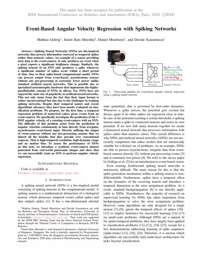
Spiking NeuralNetworkInput Spikes Angular Velocity

Event-based Camera

Fig. 1. Processing pipeline for event-based angular velocity regressionusing a spiking neural network.

state (potential), that is governed by first-order dynamics.Whenever a spike arrives, the potential gets excited butdecays again if no other spikes are registered close in time.In case of the potential reaching a certain threshold, a spikingneuron emits a spike to connected neurons and resets its ownpotential. If we now link many neurons together we createa dynamical neural network that processes information withspikes rather than numeric values. This crucial difference iswhy SNNs and artificial neural networks (ANNs) are not nec-essarily competitors but rather models that are intrinsicallysuitable for a distinct set of problems. As an example, SNNsare able to process asynchronous, irregular data from event-based cameras directly [2], without pre-processing events [3]and at extremely low power [4]. We refer to the survey paperby Gallego et al. [5] for an introduction to event-based vision.

Even training feedforward spiking neural networks isnotoriously difficult. The main reason for this is that thespike-generation mechanism within a spiking neuron is non-differentiable. Furthermore, spikes have a temporal effecton the dynamics of the receiving neuron and introduce atemporal dimension to the error assignment problem. As aresult, standard backpropagation [6] is not directly appli-cable to SNNs. Nonethelesss, the majority of research onsupervised learning for SNNs has taken inspiration frombackpropagation to solve the error assignment problem.However, some algorithms are only designed for a singleneuron [7]–[9], ignore the temporal effects of spikes [10]–[13] or employ heuristics for successful learning [14]–[17]on small-scale problems. Although SNNs are a natural fitfor spatio-temporal problems, they have largely been appliedto classification problems [11]–[13], [18]–[23], except for afew demonstrations addressing learning of spike sequences(spike-trains) [13], [18], [24]. Therefore, it is unclear whichalgorithm can successfully train multi-layer architectures fortasks beyond classification.

A. Contributions

In this work, we explore the utility of SNNs to performregression of numeric values in the continuous-time domainfrom event-based data. To the best of our knowledge, thisproblem setting has not been explored in SNN literature atthe time of the submission. The framework is illustrated infigure 1. The task of our choice is angular velocity (tilt, pan,roll rates) regression of a rotating event-camera. Successfulattempts to this task require a training algorithm that isable to perform accurate spatio-temporal error assignment.This might not be necessary for performing classificationon neuromorphic datasets and, thus, raises a challenge forSNNs.

Our problem setting offers the context to approach anumber of unanswered questions:

• How do we formulate a continuous-time, numeric re-gression problem for SNNs?

• Can current state-of-the-art SNN-based learning ap-proaches solve temporal problems beyond classifica-tion?

• What kind of architecture performs well on this task?• Can SNNs match the performance of ANNs in numeric

regression tasks?

As a first building block, we introduce a large-scale syntheticdataset from real-world scenes using a state-of-the-art event-camera simulator [25]. This dataset provides precise groundtruth for angular velocity which is used both for training andevaluation of the SNN. We use this dataset to successfullytrain a feedforward convolutional SNN architecture thatpredicts tilt, pan, and roll rates at all times with a recentlyproposed supervised-learning approach [18]. In addition tothat, we show that our network predicts accurately at the fullrange of angular velocities and extensively compare againstANN baselines designed to perform this task in discrete-time.

In summary, our contributions are:

• The introduction of a continuous-time regression prob-lem for spiking neural networks along with a datasetfor reproducibility.

• A novel convolutional SNN architecture designed forregression of numeric values.

• A detailed evaluation against state-of-the-art ANN mod-els crafted for event-based vision problems.

II. RELATED WORK

Currently, artificial neural networks are the de facto com-putational model of choice for a wide range problems, suchas classification, time series prediction, regression analysis,sequential decision making etc. Spiking neural networks addadditional biological relevance in these architectures withthe use of a spiking neuron as the distributed computationalunit. With the promise of increased computational ability[26], [27] and low power computation using neuromorphichardware [28]–[31], SNNs show their potential as compu-tational engines, especially for processing event-based datafrom neuromorphic sensors [32], [33].

5 10 15 20

u(t)

t[ms]0

Neuron Threshold, ϑ

Refractory Response

Spike

Resting potential

Synaptic weight

input spikes t

# Neuron

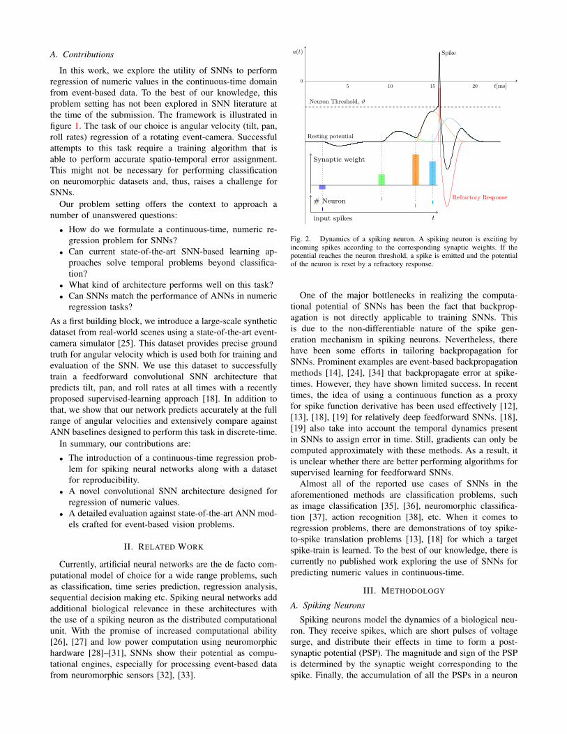
Fig. 2. Dynamics of a spiking neuron. A spiking neuron is exciting byincoming spikes according to the corresponding synaptic weights. If thepotential reaches the neuron threshold, a spike is emitted and the potentialof the neuron is reset by a refractory response.

One of the major bottlenecks in realizing the computa-tional potential of SNNs has been the fact that backprop-agation is not directly applicable to training SNNs. Thisis due to the non-differentiable nature of the spike gen-eration mechanism in spiking neurons. Nevertheless, therehave been some efforts in tailoring backpropagation forSNNs. Prominent examples are event-based backpropagationmethods [14], [24], [34] that backpropagate error at spike-times. However, they have shown limited success. In recenttimes, the idea of using a continuous function as a proxyfor spike function derivative has been used effectively [12],[13], [18], [19] for relatively deep feedforward SNNs. [18],[19] also take into account the temporal dynamics presentin SNNs to assign error in time. Still, gradients can only becomputed approximately with these methods. As a result, itis unclear whether there are better performing algorithms forsupervised learning for feedforward SNNs.

Almost all of the reported use cases of SNNs in theaforementioned methods are classification problems, suchas image classification [35], [36], neuromorphic classifica-tion [37], action recognition [38], etc. When it comes toregression problems, there are demonstrations of toy spike-to-spike translation problems [13], [18] for which a targetspike-train is learned. To the best of our knowledge, there iscurrently no published work exploring the use of SNNs forpredicting numeric values in continuous-time.

III. METHODOLOGY

A. Spiking Neurons

Spiking neurons model the dynamics of a biological neu-ron. They receive spikes, which are short pulses of voltagesurge, and distribute their effects in time to form a post-synaptic potential (PSP). The magnitude and sign of the PSPis determined by the synaptic weight corresponding to thespike. Finally, the accumulation of all the PSPs in a neuron

constitutes the sub-threshold membrane potential u(t). Thisprocess is illustrated in figure 2 via spikes from multiplesynapses. When the sub-threshold membrane potential isstrong enough to exceed the neuron threshold ϑ the spikingneuron responds with a spike. Immediately after the spike,the neuron tries to suppress its membrane potential sothat the spiking activity is regulated. This self-suppressionmechanism is called refractory response.

There are various mathematical models in neurosciencethat describe the dynamics of a spiking neuron with varyingdegree of detail: from the complex Hodgkin-Huxley neuron[39] to the simple Leaky Integrate and Fire neuron [1], [40].In this paper, we use the Spike Response Model (SRM)[41]. In SRM, the PSP response is a decoupled, normalizedspike response kernel, ε(t), scaled by the synaptic weight.Similarly, the refractory response is described by a refractorykernel, ν(t). The SRM is simple, yet versatile enough to rep-resent various spiking neuron characteristics with appropriatespike response and refractory kernels.

B. Feedforward Spiking Neural Networks

In this section, we define the model of feedforward SNNsand describe how events and spikes are related.

One of the advantages of SNNs over ANNs is their abilityto process event-data from event-cameras directly. Event-cameras have independent sensors at each pixel that respondasynchronously to brightness changes. An event can be de-scribed by a tuple (x, y, t, p), where x and y are the locationof the pixel from which the event was triggered at time t.The polarity p is a binary variable that indicates whether thechange in brightness is either positive or negative. The SNNmodel in this work has two inputs (i.e. two channels) foreach pixel location to account for the polarity of the events.When an event is fed as an input to the network, we referto it as spike. A sequence of spikes is called spike train andis defined as s(t) =

∑t(f)∈F δ(t− t(f)), where F is the set

of times of the individual spikes.Our SNN model is a feedforward SNN with nl layers.

In the following definition, W (l) are the synaptic weightscorresponding to layer l and sin(t) refers to the spikes of theinput layer:

s(0)(t) = sin(t) (1)

u(l+1)(t) = W (l)(ε ∗ s(l))(t) + (ν ∗ s(l+1))(t) (2)

s(l)(t) =∑

t(f)∈{t|u(l)(t)=ϑ}

δ(t− t(f)) (3)

ω(t) = W (nl)(ε ∗ s(nl))(t) (4)

where ω is the prediction of the angular velocity. We usethe following form of spike response kernel and refractorykernel:

ε(t) =t

τse1−

tτsH(t) (5)

ν(t) = −2ϑe− tτrH(t) (6)

H(·) is the Heaviside step function; τs and τr are the timeconstants of spike response kernel and refractory kernelrespectively.

Note how the spike response kernel distributes the effectof input spikes over time (eqs. (2) & (5)), peaking sometime later and exponentially decaying after the peak. Thistemporal distribution allows interaction between two inputspikes that are within the effective temporal range of thespike response kernel, thereby allowing short term memorymechanism in an SNN. It is pivotal in allowing the networkto estimate the sensor’s movement and enables prediction ofangular velocity.

C. Network ArchitectureOur network architecture is a convolutional spiking neural

network losely inspired by state-of-the-art architectures forself-supervised ego-motion prediction [42]. It consists offive convolutional layers followed by a pooling and fullyconnected layer to predict angular velocities. The first 4 con-volutional layers perform spatial downsampling with stride2. At the same time, the number of channels is doubled witheach layer starting with 16 channels in the first layer. TableI shows these layer-wise hyperparameters in more detail.It can be seen that there is another set of hyperparametersthat are time constants concerned with the decay rate of thespike response and refractory kernels in equation (5) and (6).These time constants are increasing with network depth toaccount for both high event rate from the event-camera atthe input and slower dynamics at the output for consistentpredictions. Table I lists these layer-wise hyperparameters ofthe architecture in more detail.

1) Global Average Spike Pooling (GASP): So far, the dis-cussed elements of our architecture are regularly encounteredin literature of both spiking and artificial neural networks.In recent years, global average pooling [43] has becomeprevalent in modern network architectures [44], [45] due totheir regularization effect. We adapt this line of work forspiking neural networks and introduce global average spikepooling after the last convolutional layer.

To describe GASP, we define a spatial spike-trainSi(t, x, y) resulting from the i-th channel of the previouslayer as

Si(t, x, y) =∑

t(f)∈Fi(x,y)

δ(t− t(f)), (7)

where Fi(x, y) is the set of spike times in the i-th channelat the spatial location (x, y). Let gi(t) be the i-th output ofthe pooling operation, then

gi(t) =∑

x∈{0,...,W−1}y∈{0,...,H−1}

Si(t, x, y), (8)

where W and H are width and height of the previouschannel. Successive synapses connected to the spike-traingi(t) are then scaled by 1/W ·H to introduce invariance withrespect to the spatial resolution.

After the spike-train pooling, a fully connected layer con-nects the spike-trains to three, non-spiking, output neurons

for regressing the angular velocity continuously in time. Tosummarize the computation after the pooling layer, we canreformulate the angular velocity prediction in equation (4)as

ω(t) =1

N

(ε ∗W [g1, . . . , gC ]

>)(t) (9)

where N =W ·H is the number of neurons per channel inthe last convolutional layer with C channels.

D. Synthetic Dataset Generation

Supervised learning of spiking neural networks requiresa large amount of data. In our case, we seek a datasetthat contains events from an event-camera with ground truthangular velocity. The three main criteria of our dataset arethe following: First, there must be a large variety of scenesto avoid overfitting to specific visual patterns. Second, thedataset must be balanced with respect to the distributionof angular velocities. Third, precise ground truth at hightemporal resolution is required. To the best of our knowledge,such a dataset is currently not available. As a consequence,we generate our own dataset.

To fulfill all three criteria, we generated a syntheticdatasets using ESIM [25] as an event-camera simulator.ESIM renders images along a trajectory and interpolates abrightness signal to yield an approximation of the intensityper pixel at all times. This signal is then used to generateevents with a user-chosen contrast threshold. We selectedthe contrast threshold to be normally distributed with mean0.45 and standard deviation of 0.05. Furthermore, we setthe resolution to 240 × 180 to match the resolution of theDAVIS240C event-camera [46].

As a next step, we selected a subset of 10000 panoramaimages of the Sun360 dataset [47]. From these images,ESIM simulated sequences with a temporal window of 500milliseconds each. This amounts to approximately 1.4 hoursof simulated data. The random rotational motion used togenerate this data was designed to cover all axes equallysuch that, over the whole dataset, angular velocities areuncorrelated and their mean is zero.

Finally, the dataset is divided into 9000 sequences fortraining and 500 sequences each for validation and testing.

E. Loss Function

The loss function L is defined as the time-integral overthe euclidean distance between the predicted angular velocityω(t) and ground truth angular velocity ω(t):

L =1

T1 − T0

∫ T1

T0

√e(t)>e(t) dt (10)

where e(t) = ω(t) − ω(t). The error function is notimmediately evaluated at the beginning of the simulationbecause the SNN has a certain settling time due to itsdynamics. Note that this loss function is closely related to thevan Rossum distance [48] which has been used for measuringdistances between spike-trains.

F. Training Procedure

SNNs are continuous-time dynamical system and, as such,must be discretized for simulation on GPUs. In the idealcase, we choose the discretization time steps as small aspossible for accurate simulation. In practice, however, thestep size is a trade-off between accuracy of the simulationand availability of memory and computational resources. Wechose to restrict the simulation time to 100 milliseconds witha time step of one millisecond. The loss is then evaluatedfrom 50 milliseconds onwards to avoid punishing settlingtime with less than 50 milliseconds duration.

The training of our SNNs is based on first-order optimiza-tion methods. As a consequence, we must compute gradientsof the loss function with respect to the parameters of theSNN. This is done with the publicly available1 PyTorchimplementation of SLAYER [18].

We augment the training data by performing randomhorizontal and vertical flipping and inversion of time tomitigate overfitting. The networks are then trained on the fullresolution (240 × 180) of the dataset for 240,000 iterationsand batch size of 16. The optimization method of choice isADAM [49] with a learning rate of 0.0001 without weightdecay.

IV. EXPERIMENTS

In this section, we assess the performance of our methodon the dataset described in section III-D to investigate thefollowing questions:• What is the relation between angular velocity and

prediction accuracy?• Are the predictions for tilt, pan and roll rates of com-

parable accuracy?• Is our method competitive with respect to artificial

neural networks?

A. Experimental Setup

For the purpose of evaluating the prediction accuracy ofdifferent methods, we split the test set into 6 subsets eachcontaining a specific range of angular velocities. The testset itself is generated in identical fashion to the training andvalidation set. More importantly, the panorama images, fromwhich the event data of the test set is generated, are unique tothe test set. What makes this dataset especially challenging isthe fact that the angular velocity is not initialized at zero butrather at a randomly generated initial velocity. The angularvelocity slightly varies within the generated sequence butdoes not change drastically.

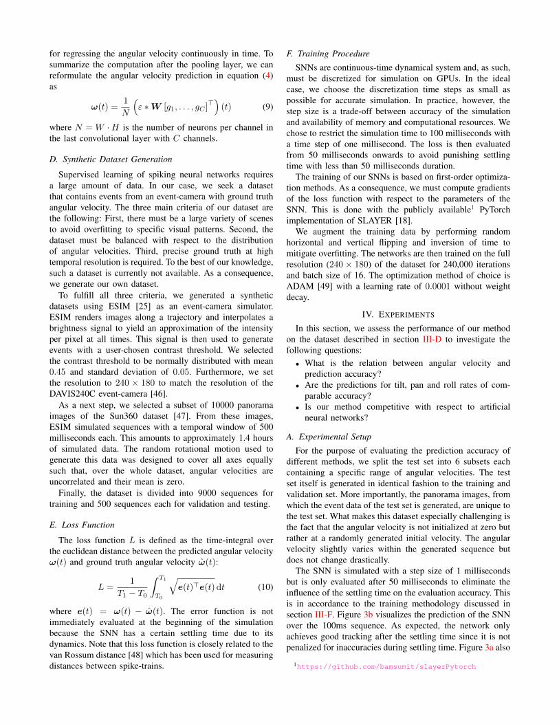
The SNN is simulated with a step size of 1 millisecondsbut is only evaluated after 50 milliseconds to eliminate theinfluence of the settling time on the evaluation accuracy. Thisis in accordance to the training methodology discussed insection III-F. Figure 3b visualizes the prediction of the SNNover the 100ms sequence. As expected, the network onlyachieves good tracking after the settling time since it is notpenalized for inaccuracies during settling time. Figure 3a also

1https://github.com/bamsumit/slayerPytorch

TABLE IHYPERPARAMETERS OF THE SPIKING NEURAL NETWORK ARCHITECTURE.

Layer-type Conv 1 Conv 2 Conv 3 Conv 4 Conv 5 Fully connected

Kernel size 3× 3 3× 3 3× 3 3× 3 3× 3 -Channels 16 32 64 128 256 -Stride 2 2 2 2 1 -τs, τr [ms] 2, 1 2, 1 4, 4 4, 4 4, 4 8, -

(a)

0 20 40 60 80 100time [ms]

0

100

200

300

400

Ang

ular

velo

city

[deg

/s]

prediction: ωtiltpanroll

ground truth: ωtiltpanroll

(b)

Fig. 3. (a): Events over the 100ms test sequence. Positive events in red and negative events in blue. (b) Continuous-time angular velocity predictionsby the SNN and the corresponding ground truth. The SNN requires a settling time of around 50 milliseconds which is exactly when the loss function isapplied while training the network. ‘Pred’ refers to prediction and ‘gt’ refers to ground truth.

shows the space-time volume of events that are fed to theSNN for the same sequence.

We also compare our method against three feedforwardartificial neural networks. Architecture ANN-6 is based onthe same architecture as the 6-layer SNN (SNN-6) specifiedin table I (with ReLU activation functions). To examinethe importance of deeper networks we train two ResNet-50architectures [44]. The only difference between them is thatone is trained with inputs consisting of two-channel framescomputed by accumulating events [50], denoted by (a), whilethe other is trained with inputs computed by drawing eventsinto a voxel-grid [3], denoted by (V). ANN-6 is only trainedwith the voxel-grid representation.

Feedforward ANNs cannot continuously predict angularvelocity2. As a consequence, the training of the ANNs isbased on minimizing the error of the mean angular velocitywithin a time window of 20 ms. Subsequently, the timewindow is shifted to the next non-overlapping sequence ofevents. In a similar fashion, ANN predictions are evaluatedevery 20 ms for comparison with the SNN.

B. Quantitative Evaluation

Figure 4 reports the median of the relative error over therange of angular velocities in the test set for all trainedmodels. All models tend to have high relative error at slow

2It is theoretically possible to shift the time window for very smallincrements at the expense of computational costs

angular velocity. Note, however, that achieving low relativeerror at low absolute speed is difficult in general due tothe fact that the relative error is infinite in the limit ofzero angular velocity. Overall, the 6-layer SNN performscomparably to the ANN-6 and the ResNet-50 (A) baselinewhile ResNet-50 (V) with the voxel-based representationachieves the lowest error in general. These findings arecondensed in table II which additionally provides the RMSEand median of relative errors of the naive mean3 predictionbaseline.

Next, we investigate the impact of angular velocities ontilt, pan and roll rates separately. Figure 5 shows the boxplots of the relative errors4 with respect to different angularvelocities. Across the whole range of angular velocities,predictions for tilt are slightly more accurate than those forpan while the error for roll is in general higher than comparedto the other axes.

C. DiscussionIn summary, the SNN is able to regress angular velocity

with reasonable accuracy across different rates. The 6-layerANN achieves only slightly lower error than the SNN. Fromthis result we conclude that it is possible to train SSNs toANN-competitive accuracy on this continuous-time regres-sion task. The slightly lower performance could originate

3Arithmetic mean of the training dataset which is close to zero4defined as ωi−ωi

|ωi|, with i for either the tilt, pan or roll axis

[0,120) [120,240) [240,360) [360,480) [480,600) [600,∞)

Angular velocity ||ω || [deg/s]

0.0

0.1

0.2

0.3

0.4

0.5

Med

ian

rela

tive

erro

r||ω

pred−

ωgt||·||ω

gt||−

1 SNN-6ANN-6 (V)ResNet-50 (A)ResNet-50 (V)

Fig. 4. Median relative errors on the test set for different angular velocitiesfor all trained models. [ωa, ωb) indicates that angular velocities in the rangeof ωa and ωb are considered. The SNN achieves comparable accuracy to itsANN counterpart with 6 layers. Both are outperformed by ResNet-50 withthe voxel-based input representation (V). In contrast, the same network withaccumulation-based input (A) achieves errors on the order of ANN-6 andSNN-6. This highlights that the lack of accurate input representation cannotbe compensated with increasing the number of layers in the network.

[0,120) [120,240) [240,360) [360,480) [480,600) [600,∞)Angular velocity ||ω || [deg/s]

−2

−1

0

1

2

Rel

ativ

edi

ffer

ence

erro

r

tiltpanroll

Fig. 5. Quartiles of the relative difference errors of SNN predictions on thetest set. The difference between prediction and groundtruth is normalizedwith respect to the absolute value of the ground truth tilt, pan or roll ratesrespectively. Evidently, the SNN is performing better at moderate to highangular rates while the roll predictions are in general less accurate than tiltand pan.

from potentially suboptimal hyperparameters for spike andrefractory response (τs and τr in table I). These parameterscould potentially be learned as well but this is left to futurework.

The large discrepancy between the error achieved by thetwo ResNet architectures are due to their difference in theinput representation. Unlike the voxel-based representation,the accumulation-based representation completely discardstimings of the events. This appears to be problematic forregression of angular velocity. On the other hand, the sig-nificant jump in accuracy from ANN-6 to ResNet-50, bothwith voxel-based input, suggests that the SNN could alsobenefit from increasing the number of layers. Nevertheless,we expect that optimizing deeper SNNs might uncover newchallenges for currently popular training methods [12], [18].

Our axis-isolating experiments suggest that predicting

roll rate is more challenging for the SNN than predictingtilt and pan rates. Similar observations were made for anoptimization-based approach to angular rate tracking [51].When the camera is being rolled, events are typically trig-gered at the periphery. The resulting spatial-temporal patternsare spread over the whole frame, which poses difficulties forour architecture.

TABLE IIBASELINE COMPARISONS ON THE TEST SET: THE SNN IS COMPARED

AGAINST THE ANN MODELS AND THE NAIVE MEAN PREDICTION

BASELINE. INPUT REPRESENTATIONS ARE EITHER EVENT-BASED (E),ACCUMULATION-BASED (A) [50] OR VOXEL-BASED (V) [3].

mean SNN-6 ANN-6 ResNet-50

Relative error 1.00 0.26 0.22 0.22 0.15RMSE (deg/s) 226.9 66.3 59.0 66.8 36.8Input type - E V A V

V. CONCLUSION

In this work, we investigated the applicability of feed-forward SNNs to regress angular velocities in continuous-time. We showed that it is possible to train a spiking neuralnetwork to perform this task on par with artificial neuralnetworks. Thus, we can confirm that state-of-the-art SNNtraining procedures accurately address the temporal errorassignment problem for SNNs of the size as presented in thiswork. Experimental results further suggest that deeper SNNsmight perform significantly better, but there are a number ofobstacles ahead. Backpropagation-based approaches requirethat we unroll the SNN in time at high-resolution. Thisrequirement poses serious challenges for optimization onGPUs both in terms of memory consumption and FLOPS. Ithas been a long-standing research goal to address these issuesand we believe it to be crucial to unlock the full potential ofSNNs.

REFERENCES

[1] W. Gerstner and W. M. Kistler, Spiking neuron models: Single neurons,populations, plasticity. Cambridge university press, 2002.

[2] G. K. Cohen, G. Orchard, S.-H. Leng, J. Tapson, R. B. Benosman,and A. Van Schaik, “Skimming digits: neuromorphic classification ofspike-encoded images,” Frontiers in neuroscience, vol. 10, p. 184,2016.

[3] D. Gehrig, A. Loquercio, K. G. Derpanis, and D. Scaramuzza, “End-to-end learning of representations for asynchronous event-based data,”in Proceedings of the IEEE International Conference on ComputerVision, pp. 5633–5643, 2019.

[4] S. Moradi, N. Qiao, F. Stefanini, and G. Indiveri, “A scalable multicorearchitecture with heterogeneous memory structures for dynamic neu-romorphic asynchronous processors (DYNAPs),” IEEE Trans. Biomed.Circuits Syst., vol. 12, no. 1, pp. 106–122, 2018.

[5] G. Gallego, T. Delbruck, G. Orchard, C. Bartolozzi, B. Taba,A. Censi, S. Leutenegger, A. Davison, J. Conradt, K. Daniilidis,and D. Scaramuzza, “Event-based vision: A survey,” arXiv e-prints,vol. abs/1904.08405v2, 2019.

[6] D. E. Rumelhart, G. E. Hinton, and R. J. Williams, “Learningrepresentations by back-propagating errors,” Nature, vol. 323, pp. 533–536, 1986.

[7] F. Ponulak, “ReSuMe-new supervised learning method for spikingneural networks,” Institute of Control and Information Engineering,Poznan University of Technology., 2005.

[8] A. Mohemmed, S. Schliebs, S. Matsuda, and N. Kasabov, “Span: Spikepattern association neuron for learning spatio-temporal spike patterns,”International Journal of Neural Systems, vol. 22, no. 04, p. 1250012,2012. PMID: 22830962.

[9] R. Gutig and H. Sompolinsky, “The tempotron: a neuron that learnsspike timing–based decisions,” Nature neuroscience, vol. 9, no. 3,pp. 420–428, 2006.

[10] J. H. Lee, T. Delbruck, and M. Pfeiffer, “Training deep spiking neuralnetworks using backpropagation,” Frontiers in Neuroscience, vol. 10,p. 508, 2016.

[11] Y. Jin, W. Zhang, and P. Li, “Hybrid macro/micro level backprop-agation for training deep spiking neural networks,” in Advances inNeural Information Processing Systems 31 (S. Bengio, H. Wallach,H. Larochelle, K. Grauman, N. Cesa-Bianchi, and R. Garnett, eds.),pp. 7005–7015, Curran Associates, Inc., 2018.

[12] E. O. Neftci, H. Mostafa, and F. Zenke, “Surrogate gradient learningin spiking neural networks: Bringing the power of gradient-basedoptimization to spiking neural networks,” IEEE Signal ProcessingMagazine, vol. 36, no. 6, pp. 51–63, 2019.

[13] F. Zenke and S. Ganguli, “SuperSpike: Supervised Learning inMultilayer Spiking Neural Networks,” Neural Computation, vol. 30,pp. 1514–1541, Apr. 2018.

[14] S. M. Bohte, J. N. Kok, and H. La Poutre, “Error-backpropagation intemporally encoded networks of spiking neurons,” Neurocomputing,vol. 48, no. 1, pp. 17–37, 2002.

[15] O. Booij and H. tat Nguyen, “A gradient descent rule for spikingneurons emitting multiple spikes,” Information Processing Letters,vol. 95, no. 6, pp. 552 – 558, 2005. Applications of Spiking NeuralNetworks.

[16] S. B. Shrestha and Q. Song, “Robust learning in SpikeProp,” NeuralNetworks, vol. 86, pp. 54 – 68, 2017.

[17] S. B. Shrestha and Q. Song, “Robustness to training disturbancesin SpikeProp learning,” IEEE Transactions on Neural Networks andLearning Systems, vol. PP, pp. 1–14, July 2017.

[18] S. B. Shrestha and G. Orchard, “SLAYER: Spike layer error reassign-ment in time,” in Advances in Neural Information Processing Systems31 (S. Bengio, H. Wallach, H. Larochelle, K. Grauman, N. Cesa-Bianchi, and R. Garnett, eds.), pp. 1419–1428, Curran Associates,Inc., 2018.

[19] Y. Wu, L. Deng, G. Li, J. Zhu, and L. Shi, “Spatio-temporal back-propagation for training high-performance spiking neural networks,”Frontiers in Neuroscience, vol. 12, p. 331, 2018.

[20] A. Tavanaei, M. Ghodrati, S. R. Kheradpisheh, T. Masquelier, andA. Maida, “Deep learning in spiking neural networks,” Neural Net-works, vol. 111, pp. 47 – 63, 2019.

[21] S. K. Esser, P. A. Merolla, J. V. Arthur, A. S. Cassidy, R. Appuswamy,A. Andreopoulos, D. J. Berg, J. L. McKinstry, T. Melano, D. R.Barch, C. di Nolfo, P. Datta, A. Amir, B. Taba, M. D. Flickner,and D. S. Modha, “Convolutional networks for fast, energy-efficientneuromorphic computing,” Proceedings of the National Academy ofSciences, vol. 113, no. 41, pp. 11441–11446, 2016.

[22] P. U. Diehl, D. Neil, J. Binas, M. Cook, S.-C. Liu, and M. Pfeiffer,“Fast-classifying, high-accuracy spiking deep networks through weightand threshold balancing,” in 2015 International Joint Conference onNeural Networks (IJCNN), pp. 1–8, IEEE, 2015.

[23] B. Rueckauer, I.-A. Lungu, Y. Hu, M. Pfeiffer, and S.-C. Liu, “Con-version of continuous-valued deep networks to efficient event-drivennetworks for image classification,” Frontiers in Neuroscience, vol. 11,p. 682, 2017.

[24] S. B. Shrestha and Q. Song, “Event based weight update for learninginfinite spike train,” in 2016 15th IEEE International Conference onMachine Learning and Applications (ICMLA), pp. 333–338, Dec 2016.

[25] H. Rebecq, D. Gehrig, and D. Scaramuzza, “ESIM: an open eventcamera simulator,” in Conf. on Robotics Learning (CoRL), 2018.

[26] W. Maass, “Lower bounds for the computational power of networksof spiking neurons,” Neural Computation, vol. 8, pp. 1–40, Jan. 1996.

[27] W. Maass, “Noisy spiking neurons with temporal coding have morecomputational power than sigmoidal neurons,” in Advances in NeuralInformation Processing Systems 9, NIPS, Denver, CO, USA, December2-5, 1996 (M. Mozer, M. I. Jordan, and T. Petsche, eds.), pp. 211–217,MIT Press, 1996.

[28] M. Davies, N. Srinivasa, T.-H. Lin, G. Chinya, Y. Cao, S. H. Choday,G. Dimou, P. Joshi, N. Imam, S. Jain, et al., “Loihi: A neuromorphicmanycore processor with on-chip learning,” IEEE Micro, vol. 38, no. 1,pp. 82–99, 2018.

[29] P. A. Merolla, J. V. Arthur, R. Alvarez-Icaza, A. S. Cassidy, J. Sawada,F. Akopyan, B. L. Jackson, N. Imam, C. Guo, Y. Nakamura, B. Brezzo,I. Vo, S. K. Esser, R. Appuswamy, B. Taba, A. Amir, M. D. Flickner,W. P. Risk, R. Manohar, and D. S. Modha, “A million spiking-neuron integrated circuit with a scalable communication network andinterface,” Science, vol. 345, no. 6197, pp. 668–673, 2014.

[30] A. Neckar, S. Fok, B. V. Benjamin, T. C. Stewart, N. N. Oza, A. R.Voelker, C. Eliasmith, R. Manohar, and K. Boahen, “Braindrop: Amixed-signal neuromorphic architecture with a dynamical systems-based programming model,” Proceedings of the IEEE, vol. 107,pp. 144–164, Jan 2019.

[31] S. B. Furber, F. Galluppi, S. Temple, and L. A. Plana, “The spinnakerproject,” Proceedings of the IEEE, vol. 102, no. 5, pp. 652–665, 2014.

[32] P. Lichtsteiner and T. Delbruck, “A 64x64 AER logarithmic temporalderivative silicon retina,” in Research in Microelectronics and Elec-tronics, PhD, vol. 2, pp. 202–205, 2005.

[33] V. Chan, S.-C. Liu, and A. van Schaik, “Aer ear: A matched siliconcochlea pair with address event representation interface,” IEEE Trans-actions on Circuits and Systems I: Regular Papers, vol. 54, no. 1,pp. 48–59, 2007.

[34] B. Schrauwen and J. Van Campenhout, “Improving spikeprop enhance-ments to an error-backpropagation rule for spiking neural networks,”in Proceedings of the 15th prorisc workshop, vol. 11, 2004.

[35] Y. Lecun, L. Bottou, Y. Bengio, and P. Haffner, “Gradient-basedlearning applied to document recognition,” Proceedings of the IEEE,vol. 86, pp. 2278–2324, Nov 1998.

[36] A. Krizhevsky et al., “Learning multiple layers of features from tinyimages,” tech. rep., Citeseer, 2009.

[37] G. Orchard, A. Jayawant, G. K. Cohen, and N. Thakor, “Convertingstatic image datasets to spiking neuromorphic datasets using saccades,”Frontiers in Neuroscience, vol. 9, p. 437, 2015.

[38] A. Amir, B. Taba, D. Berg, T. Melano, J. McKinstry, C. di Nolfo,T. Nayak, A. Andreopoulos, G. Garreau, M. Mendoza, J. Kusnitz,M. Debole, S. Esser, T. Delbruck, M. Flickner, and D. Modha, “Alow power, fully event-based gesture recognition system,” in The IEEEConference on Computer Vision and Pattern Recognition (CVPR), July2017.

[39] A. L. Hodgkin and A. F. Huxley, “A quantitative description ofmembrane current and its application to conduction and excitationin nerve,” The Journal of physiology, vol. 117, no. 4, p. 500, 1952.

[40] H. Paugam-Moisy and S. M. Bohte, Handbook of Natural Computing,vol. 1, ch. Computing with Spiking Neuron Networks, pp. 335–376.Springer Berlin Heidelberg, 1st ed., 2011.

[41] W. Gerstner, “Time structure of the activity in neural network models,”Phys. Rev. E, vol. 51, pp. 738–758, Jan 1995.

[42] A. Gordon, H. Li, R. Jonschkowski, and A. Angelova, “Depth fromvideos in the wild: Unsupervised monocular depth learning from un-known cameras,” in Proceedings of the IEEE International Conferenceon Computer Vision, pp. 8977–8986, 2019.

[43] M. Lin, Q. Chen, and S. Yan, “Network in network,” in ICLR, 2014.[44] K. He, X. Zhang, S. Ren, and J. Sun, “Deep residual learning for image

recognition,” in Proceedings of the IEEE conference on computervision and pattern recognition, pp. 770–778, 2016.

[45] K. Simonyan and A. Zisserman, “Very deep convolutional networksfor large-scale image recognition,” in International Conference onLearning Representations, 2015.

[46] C. Brandli, R. Berner, M. Yang, S.-C. Liu, and T. Delbruck, “A 240×180 130 db 3 µs latency global shutter spatiotemporal vision sensor,”IEEE Journal of Solid-State Circuits, vol. 49, no. 10, pp. 2333–2341,2014.

[47] J. Xiao, K. A. Ehinger, A. Oliva, and A. Torralba, “Recognizing sceneviewpoint using panoramic place representation,” in cvpr, pp. 2695–2702, IEEE, 2012.

[48] M. v. Rossum, “A novel spike distance,” Neural computation, vol. 13,no. 4, pp. 751–763, 2001.

[49] D. P. Kingma and J. Ba, “Adam: A method for stochastic optimiza-tion,” in International Conference on Learning Representations, 2014.

[50] A. I. Maqueda, A. Loquercio, G. Gallego, N. Garcıa, and D. Scara-muzza, “Event-based vision meets deep learning on steering predictionfor self-driving cars,” in IEEE Conf. Comput. Vis. Pattern Recog.(CVPR), pp. 5419–5427, 2018.

[51] G. Gallego and D. Scaramuzza, “Accurate angular velocity estimationwith an event camera,” IEEE Robot. Autom. Lett., vol. 2, pp. 632–639,2017.