evaluation of topographic index in relation to terrain

Evaluation of topographic index in relation to terrainroughness and DEM grid spacing

Samadrita Mukherjee1, Sandip Mukherjee

1,∗, R D Garg2, A Bhardwaj

3 and P L N Raju3

1National Technical Research Organisation, Govt. of India, Delhi 110 001, India.2Department of Civil Engineering, Indian Institute of Technology, Roorkee 247 667, India.

3Indian Institute of Remote Sensing, Indian Space Research Organisation, Dehradun 248 001, India.∗Corresponding author. e-mail: [email protected]

Topographic index is an important attribute of digital elevation model (DEM) which indicates soil satu-ration. It is used for estimation of run-off, soil moisture, depth of ground water and hydrological simula-tion. Topographic index is derived from DEMs; hence the accuracy of DEM influences its computation.Commonly the raster based grid DEM is widely used to simulate hydrological model parameter, andaccuracy varies with respect to DEM grid size and morphological characteristics of terrain. In this studytopographic index is evaluated in terms of DEM grid size and terrain roughness. The study was car-ried out on four small watersheds, having different roughness characteristics, located over the Himalayanterrain. Topographic index surface is derived for each watershed from different grid spacing DEM (10–150 m), analysed and validated. It is found that DEM grid spacing affects the topographic index. Thesurface representation is smooth in the coarse grid spacing and the pattern of topographic index changeswith grid spacing. The spatial autocorrelation of topographic index surface reduces when calculatedfrom larger spacing DEM. The mean of the topographic index surface increases and standard deviationdecreases with the increase of grid spacing and the effect is more pronounced in the rough terrain. Accu-racy of the topographic index is also evaluated with respect to grid spacing and terrain roughness bycomparing the topographic index surface with respect to reference data (10 m grid spacing topographicindex surface). The RMSE and mean error of topographic index surface increases in larger grid spacingand the effect is more in rugged terrain.

1. Introduction

Terrain relief is the first order control on the vari-ous natural process of any watershed. It influencesgravity and movement of water in a catchment andtherefore it must be taken into account in mod-elling like flow path of the run-off, distribution ofsoil moisture and depth of the ground water level,etc. (Wolock and Price 1994). Digital elevationmodel (DEM) is an approximation of continuousground surface and commonly used for the repre-sentation of terrain relief (Demoulin et al. 2007;

Yue et al. 2007; Saadat et al. 2008; Dragut andEisank 2011). It is a quantitative representationof the Earth’s surface and is typically given in oneof the three formats: grid DEM, elevation in atriangulated irregular network (TIN) and digi-tal contour. Grid DEM has been widely used tocharacterize the terrain relief for simulation ofhydrological process. The information required forsimulation can be derived from DEM in termsof primary and secondary attributes. The pri-mary attributes are slope, aspect, profile curva-ture, catchment area and the secondary attributes

Keywords. Topographic index; terrain roughness; grid spacing; DEM; Cartosat-1; spatial autocorrelation.

J. Earth Syst. Sci. 122, No. 3, June 2013, pp. 869–886c© Indian Academy of Sciences 869

870 Samadrita Mukherjee et al.

are upslope area, topographic index, stream powerindex, radiation index and temperature index(Wilson and Gallant 2000; Kennelly 2008).

Topographic index (TI) is an important para-meter for natural resource management. It is usedfor predictive vegetation modelling (Van Niel et al.2004), potential distribution of rainforest struc-tural characteristics (Mackey 1994), spatial distri-bution of soil water (Gomez-Plaza et al. 2001),prediction for plant species number for biodiversitymanagement (Zinko et al. 2005), spatial organiza-tion of soil moisture (Grayson et al. 1997; Westernet al. 1999, 2004), mapping of soil organic mat-ter (Pei et al. 2010), classification of landform ele-ments from DEM (Irvin et al. 1997), mappingof landslide susceptibility (Yesilnacar and Topal2005), identifying the relationship between cropyield and topographic variation (Si and Farrell2004), assessment of fire severity and species diver-sity (Wimberly and Reilly 2007), identification ofground water recharge influencing factor (Nolanet al. 2007), mapping of forest using classificationof topo-climatic data (Burrough et al. 2001), etc.

Topographic index is also important in the fieldof hydrological modelling. It is a popular meansto hydrologists to parameterize or characterizethe terrain relief (Chappell et al. 2006; Kakemboet al. 2007). Topographic index has been intro-duced by Beven and Kirkby (1979) in their ‘Topog-raphy based Watershed Model’ (TOPMODEL) forcharacterizing the distribution of moisture statusin a basin (Quinn and Beven 1993; Huang andJiang 2002; Hjerdt et al. 2004; Tombul 2007).The effect of terrain relief on watershed hydrol-ogy is represented in TOPMODEL as the spa-tial distribution of the topographic index. Anotherhydrological model ‘TOPOG’ examines the pat-tern of surface saturation using the topographicindex (O’Loughlin 1986). Topographic index is acompound terrain attribute, computed from spe-cific catchment area of a point and the local slope(Schmidt and Persson 2003). It reflects the spatialdistribution of soil saturation (Beven and Kirkby1979) and indicates the accumulated water flowat any point in a catchment. A high value of thetopographic index indicates the region has higherpotential to be saturated (Raaflaub and Collins2006). A high value of upslope drainage area andlow slope results in a high topographic index, hencea high probability of occurrence of soil saturation.

Many studies used the topographic index sinceyear 1979 and modification has been done byresearchers dealing with three types of topographicindices:

(i) Topographic Index: Ln(α/tan β) also knownas ‘Wetness Index’ or ‘TOPMODEL topo-graphic index’, where α (specific catchment

area) represents upslope area per unit contourlength which means the area above a certaincontour that contributes flow across the con-tour. It indicates the amount of water thatcan flow through location. For grid data, con-tour length is equivalent to grid spacing, andtan β is local down slope (Raaflaub and Collins2006).

(ii) Soil topographic index: Log(α/T tan β) whereα is drainage area per unit contour length andT is lateral transmissivity of soil (Merot et al.2003).

(iii) Climato-topographic index: Log(V r/tanβ)where Vr is volume of annual precipitation(Merot et al. 2003).

Topographic index is derived from a DEM. Likeother spatial datasets, DEMs are subjected to dif-ferent types of errors such as gross errors dur-ing data collection, deficient orientation of stereoimages (systematic error) when photogrammet-rically determining elevation values, transforma-tion method of control points, mathematical modelused for construction of surface and random error.The other issues related to DEM accuracy are gridspacing, interpolation techniques used and mor-phological characteristics of terrain (Tempfli 2000;Yue et al. 2007). Hence, the errors associated withthe DEMs affect the accuracy of the topographicindex (Peifa et al. 2006). Researchers have anal-ysed the various properties of topographic index.Vaze et al. (2010) studied the effect of DEM gridspacing on topographic indices and found thatthe slight change in maximum and minimum ele-vation and substantial change in elevation differ-ence in the coarser spacing DEM. The mean ofslope decreases and variation in calculation of hill-shade and stream network are found in coarsegrid spacing DEM. Mean of topographic indexincreases progressively with DEM grid spacingwhich negatively affects the efficiency of model pre-diction (Brasington and Richards 1998). Zhang andMontgomery (1994) found that as topographicindex value increases progressively in higher gridspacing, the percentage of predicted saturated areacalculation also increased. Significant differencewas found in the spatial pattern of topographicindex computed from 5 to 50 m grid spacing DEMs(Quinn et al. 1991). Wolock and Price (1994)generated the elevation model from 1:24,000 and1:250,000 scale toposheets and compared the effectof both DEMs map scale and data resolution onthe statistics of topographic index and found thatmean of topographic index increases with increaseof grid size. The effect of DEM error on topographicindex was investigated by using Monte Carlo Simu-lation (Raaflaub and Collins 2006), suggestedthat error of topographic index is more sensitive to

Topographic index in relation to terrain roughness and DEM grid spacing 871

the number of neighbours used in the slope algo-rithm and the error is more along the drainagenetwork. Topographic index is used by differentresearchers considering different DEM grid spac-ing for their application at local and regional scale(Kumar et al. 2000; Wu et al. 2007). Grid spacingdirectly affects the calculation of upslope area aswell as the topographic index (Quinn et al. 1995).Yong et al. (2009) analysed the effect of terrainsmoothening and discretisation of DEM grid spac-ing on topographic index and found that smoothen-ing effect is relatively higher in the relatively cliffyterrain while discretisation effect is dominant inflat areas. The effect of smoothening and dis-cretisation were closely related to local terraincharacteristics.

However, the assessment of the topographicindex is very important because any variation inthe topographic index calculation may affect theaccuracy of its applications and outcome of themodel prediction (Raaflaub and Collins 2006). Itis also important to study the characteristics oftopographic index in Indian landscape especiallyin Himalayan terrain. In this study an attempthas been made to evaluate the topographic index(TOPMODEL topographic index) in ShivalikHimalayan terrain considering DEM grid spac-ing and terrain ruggedness characteristics. The

study analyse how the DEM grid spacing and ter-rain roughness affect the statistical properties andaccuracy of topographic index.

2. Study area

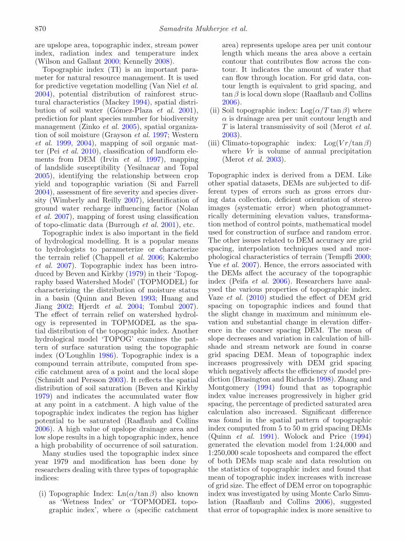
Western part of Dehradun, India is taken as thestudy area which is geographically situated within30◦8′30′′–30◦27′3′′N and 77◦43′2′′–78◦2′52′′E(figure 1a). It is situated in the tropical (Joshiet al. 2011) climatic region, although it variesfrom warm in summers to severely cold in winters,depending upon the season and the altitude of thespecific location. The district being hilly, temper-ature variations due to difference in elevation areconsiderable. Summers (March–June) have maxi-mum temperature of 35◦C and minimum of 17◦C.Winters (December to February) have maximumof 22◦C and minimum of about 3◦C. During themonsoon season heavy rainfall occurs. The areareceives an average annual rainfall of 2100 mm.Most of the annual rainfall is received during themonths from June to September. Significant reliefvariation is present in this area. Geomorphologi-cally the area is characterized by hills and valleys.The lower middle part of the study area is highly

India

(a)

Figure 1(a). Cartosat DEM of study area and location of four drainage basins.


rugged and mainly dominated by hills. Because ofthe high slope, the area is dissected by numberof small rivers. The northern part of this area isthe foot of the Mussoorie hill, having less terrainrelief in comparison to the lower middle part.Central part of the terrain has little undulationbut southern part is completely flat (figure 1a).Type of forest is mixed; within this Sal forest isdominating and density is medium to scattered.The hilly area is partially covered by the vege-tation and very small vegetation cover is presentalong the river valley.

The present study analysed the impact of gridspacing and terrain roughness on the topographicindex. Ruggedness implies the variation of slopein a terrain. It indicates the undulation or variationof relief. In order to identify the influence of terrainroughness, four small drainage basins of differentrelief characteristics (very rough to undulated)have selected and named as per the surface rough-ness; Highly rugged, Rugged, Moderately ruggedand Undulated basin (figure 1b). For each basin,

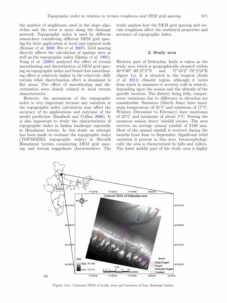
elevation versus distance curves were also plottedto understand their surface roughness characteris-tics by selecting two cross-sections (A–B and C–D) in the upper and lower portions of the basins(figure 1c). Initially the basins were identified fromthe Survey of India (SOI) toposheets and inspectedduring the field survey to segregate the basin asper relief characteristics. Qualitative and quanti-tative analysis carried out on the basin relief arediscussed in section 4.1. The boundary of drainagebasins were delineated using automatic catchmentselection algorithm and the basin outlets were iden-tified from SOI toposheet nos. 53J/3,4, 53F/15,16at 1:50,000 scale. Information of the basins is givenin table 1.

3. Material and methods

The methodology adopted in this study for assess-ment of the topographic index is given in sequentialmanner in figure 2.

(b)

Figure 1(b). Enlargement of the basins showing the relief of terrain and altitudinal variations.


Highly Rugged Basin Rugged Basin

A B

C D

A B

C D

Moderately Rugged Basin Undulated Basin

A B

C D C D

A B

(c)

Figure 1(c). Cross section of upper and lower portion of each basin showing the terrain roughness characteristics.

Table 1. Basin characteristics.

Catchment type Area (km2) Stream order Outlet elevation (m) Outlet coordinate Perimeter (m)

Highly rugged 7.06 4 495 30◦16′35′′N, 77◦46′28′′E 13551.84

Rugged 9.88 4 463 30◦10′43′′N, 77◦57′31′′E 16058.05

Moderately rugged 15.97 5 454 30◦20′39′′N, 77◦56′21′′E 25419.03

Undulated 9.13 4 442 30◦20′10′′N, 77◦52′50′′E 19176.85

3.1 DEM generation

High resolution (2.5 m) Cartosat-1 data was usedin this study. Cartosat-1 satellite has a forward(F) and aft (A) panchromatic camera which givesthe along track stereo, with a tilt of +26◦ and−5◦ respectively in flight direction (Baltsaviaset al. 2007). Stereo imagery of 2 October 2005(Path/Row – 0526/0258) was used for generationof DEM. DGPS (Differential Global PositioningSystem) survey was conducted in the Dehradunarea and 20 well distributed GCPs (ground con-trol points) over the scene were collected. Initially

stereo block was oriented with RPCs (rationalpolynomial coefficients) which comes with thesatellite data. Then GCPs were added in the stereomodel to avoid the systematic error. 15 GCPs wereused as control points and 5 GCPs were used ascheck points to orient the stereo model. LPS soft-ware, version 9.2, has been used for the orientationof the stereo block. From the oriented stereo block,DEM at 10 m grid size has been generated withoverall accuracy (RMSE) of 1.06 pixels and verti-cal check point accuracy of 1.11 m (RMSE). Afterthat from the same block DEMs at grid size 30, 50,90, 110 and 150 m were produced.


DGPS Data (raw GCPs)

Processing Using Ski-

Pro Software

Processed

GCPs

Cartosat-1 Stereo Data

Stereo Block Orientation

DEM Generation (10m, …, 150m)

Sink Filling

Sink free DEM

Upslope area

Topographic index (10m, …, 150m)

Slope

Figure 2. Flow diagram of DEM generation and calculation of topographic attributes.

3.2 Sink filling and catchment delineation

Presence of sink or artifacts is a common prob-lem for extraction of drainage network using DEM.If the elevation value of surrounded cell is higherthan a particular cell then the down slope flowpath of that cell has been confined and the sinkoccur (Grimaldi et al. 2007; Wu et al. 2008). Thesink can be real component of DEM or artifactsproduced during the DEM generation process. Itcauses difficulties in hydrological calculation andneed to be removed by increasing the values of cellin each sink by the value of cell with lowest valueon sink boundary (Jenson and Domingue 1988).Sink filling was carried out for all DEMs beforedelineation of catchment and generation of terrainattribute. After the sink filling, drainage networkwas extracted with the help of flow direction andflow accumulation and finally the catchment wasdelineated.

3.3 Computation of topographic indexAccording to the algorithm (Ln (α/tanβ)), twoparameters are needed to derive the topographic

index; specific catchment area (α) and slope(tan β).

3.3.1 Calculation of specific catchment area (α)

The calculation of specific catchment area requiresthe total area draining into each cell, i.e., upslopecontributing area and ‘contour length’. For a gridDEM ‘contour length’ is considered to be the gridspacing.

Upslope area (A) = (No. of upslope cells + 1)

× (grid cell area) (1)

Specific catchment area (α) = A/L, (2)

where L = grid spacing.Various algorithms are used for the calculation of

upslope contributing area. Among them single flowdirection algorithm (SFD) and multiple flow direc-tion algorithm (MFD) are most commonly usedby the hydrologists for modelling. SFD method(Jenson and Domingue 1988) directs water flowfrom each grid cell to one of eight nearest neighbours


based on steepest downslope direction (Wolock andMcCabe 1995). Whereas MFD algorithm assumesthat water flows from a cell to its entire downslopeneighbours with weighting by slope (Quinn et al.1991; Pan et al. 2004). SFD method is suitable forzone of convergent flow and well defined valleys,while MFD method is accurate for overland flowanalysis in hill slope (Wu et al. 2008). In this studySFD algorithm was used for calculation of upslopearea. The elevation of each grid cell was comparedwith the elevation of its octagonal neighbours andthe steepest downslope direction was assigned toeach cell.

3.3.2 Calculation of slope (tan β)

At a given point on a surface, height value is Z =f(x, y). The first derivative of elevation describesthe rate of change of elevation, which is slope.Together, slope in x direction and slope in y direc-tion (partial derivatives of z with respect to x andy directions), define gradient vector of the surface.The maximum slope can be determined by tak-ing the norm of this vector. On a grid DEM, slopecalculation is done using 3 × 3 moving windowto derive finite differential. In this study, secondorder finite difference is used. Four closest neigh-bours (FCN) algorithm (Guth 1995; Raaflaub andCollins 2006) is used for computing the slope. Ittakes into account, two orthogonal components ofslope, slope in x direction and slope in y direction.In other words, the algorithm used the four car-dinal neighbours, i.e., north, south, east and westrepresenting a second order finite difference rela-tionship. This defines the steepness and downhilldirection. The algorithm is described below:

Slope =

√(dz

dx

)2

+(

dz

dy

)2

(3)

dz

dx=

(z8 − z2)2g

,dz

dy=

(z6 − z4)2g

(4)

where dz is the difference in elevation value, dx isthe distance in x direction, dy is the distance in ydirection, z2, z4, z6, z8 are height value of 2nd, 4th,6th and 8th neighbouring cells of the central pixelof the 3 × 3 window.

4. Results and discussion

4.1 Basin relief characterization

Present study concentrated to identify the impactof terrain roughness on topographic index. Hence,the relief characteristics of the basins were anal-ysed. The roughness characteristics of the basins

were segregated based on both qualitative andquantitative analysis. For qualitative analysis,cross profile of the surface taken from 10 m gridspacing DEM and the visual interpretation of con-tour pattern of SOI toposheet (1:50,000 scale, 20 mcontour interval) were studied. Contour patternis one of the indicators of the terrain roughness.It was found that in highly rugged and ruggedbasins, the spacing of the contours was very less,indicating high slope. Also the contour lines werehighly curved implying highly varied terrain relief.Two cross sections of each basin, shown as A–Band C–D in figure 1(b), were taken in upper andlower parts of each catchment, which reflected thevariation of relief in the study area. As shown infigure 1(c), the change of elevation with respectto distance was very high in highly rugged andrugged basin. Most of the areas of these two basinswere situated above 500 m elevation and the areawas highly dissected. The roughness was more inthe upper catchment. The relief of the moderatelyrugged and undulated basins were very low andless dissected because of the few drainage line. Therelative relief of the entire profile was much lowercompared to rough terrain.

The quantitative analysis of the basin roughnesswas carried out based on three parameters:

• Surface slope,• Curvature, and• Topographic roughness index (TRI).

Roughness of the terrain can be identified bythe surface slope (change of elevation). In roughterrain, difference in elevation of an area with itsneighbourhood is high and thus rugged terrain ishaving high slope. Slope map was generated for allbasins and classified into eight classes of 10◦ equalinterval. Percentage of area within each slope classto total area of the basin was calculated and plot-ted as shown in figure 3. It was found that morethan 80% area of undulated basin, 63% of mod-erately rugged basins were having less than 10◦

slopes, while rugged and highly rugged basins havemore area in 20◦–30◦ slope category.

But slope cannot be the absolute measure of theterrain roughness because in a highly inclined ter-rain, the slope of the area may be high and thatdoes not mean the terrain is rugged. Ruggednessimplies the variation of slope in a terrain which isindicated by curvature. It determines the rate ofchange of slope along the direction at that point.A positive curvature indicates that the surface isupwardly convex and negative curvature indicatesthat the surface is upwardly concave at that cell.A value of zero indicates that the surface is flat.Profile curvature of all the four basins were calcu-lated and divided into eight classes. Percentage of


area within each class to total area of the basinswere calculated and plotted. According to the clas-sification, the area having curvature value within−0.02 to 0.02 could be considered as flat terrain.It was found (as shown in figure 4) that more than80% area of undulated basin was falling under thiscategory. In the highly rugged and rugged basins,the change of slope was more in comparison toundulated basin and thus curvature was high.

TRI was computed (Moreno et al. 2005) to seg-regate the basins as per terrain relief. TRI repre-sents the amount of elevation difference among theadjacent cells of a DEM. The process computes thedifferences in elevation value from central cell to itseight neighbours. TRI is derived by taking the root-mean-square of the elevation differences. It reflectsaverage elevation change between any point on agrid and its surrounding areas. The mean value ofTRI was taken into consideration and it was foundto be 5.34, 4.61, 1.87 and 1.26 for highly rugged,rugged, moderately rugged and undulated basins,respectively.

4.2 Effect of DEM grid spacing and terrainroughness on spatial autocorrelation

of the topographic index

Topographic index was computed for all fourdrainage basins from low to high (10–150 m) gridspacing Cartosat DEMs. It was found that compu-tation of the topographic index was affected by gridspacing of DEM. For higher grid spacing, the topo-graphic index of a catchment reflected only higherorder stream and was tend to ignore the existenceof low order channels (figure 5). Due to the highsmoothing effect at larger spacing, small channelswere ‘hidden’ within the grid cells. In smallergrid spacing, the spatial pattern of topographicindex matched with the drainage network. Nearthe drainage network, topographic index valueswere high and it declined away from the drainagelines. This reflected the spatial correlation of thetopographic index with respect to its spatial loca-tion, which was referred as spatial autocorrela-tion. But towards the large grid spacing, spatial

0

10

20

30

40

50

60

70

80

90

0-10 10-20 20-30 30-40 40-50 50-60 60-70 >70

% o

f ar

ea t

o to

tal a

rea

Slope in degree

Undulated Moderately Rugged Rugged Highly Rugged

Figure 3. Slope – % area relationship for the basins.

0

5

10

15

20

25

30

35

40

45

<-0.2 -0.2 to -0.04 -0.04 to -0.02 -0.02 to 0 0 to 0.02 0.02 to 0.04 0.04 to 0.2 >0.2

% o

f cl

ass

area

to t

otal

are

a

Curvature class

Undulate Basin Moderately Rugged Basin Rugged Basin Highly Rugged Basin

Figure 4. Profile curvature of the basins.


30 m10 m 50 m

90 m 110 m 150 m

Figure 5. Topographic index computed from 10 to 150 m grid spacing of DEM for highly rugged basin. It shows the highvalue of topographic index near the drainage line.

autocorrelation of the topographic index was vio-lated. Spatial autocorrelation index was investi-gated in terms of Moran’s I index (Dale and Fortin2002; Cai and Wang 2006; Shortridge 2007) for thetopographic index surfaces at different grid spacing(figure 6). The value of Moran’s I index varied from+1 to −1. Positive value indicated that the objectswere highly correlated or clustered whereas neg-ative value indicated the dissimilarity (Goodchild1986). It showed that Moran’s I value of topo-graphic index surfaces declined with increase inthe grid spacing which signified that pattern ofthe topographic index surface was changing andbecoming more random with the increase of gridspacing.

4.3 Effect of DEM grid spacing and terrainroughness on the topographic index statistics

It was found that grid spacing of DEM hasgreat impact on the derivation of the topographicindex. The statistics of topographic index surface(table 2) for all basins have changed with the grid

spacing. Minimum value of the topographic indexsurface has increased and the maximum valuedecreased with higher grid spacing. The range andstandard deviation values were also found to be lesswhen the topographic index was computed fromDEMs with larger grid spacing. It was also foundthat grid spacing has significant impact on themean of topographic index. Mean of topographicindex was continuously increasing with increase ingrid spacing (figure 7). Mean of topographic indexplot showed that the overall trend of the curveswas parabolic in nature, but up to 90 m resolu-tion this trend was found close to linear function.It was observed that mean of topographic indexwas more in the undulated basin in comparison torugged basin, because the smooth area was hav-ing more potential to be saturated due to lowerground slope and the potentiality of soil satura-tion and topographic index both would be higher.If the grid spacing of DEM was increased, the rep-resentation of surface became smoother. A smoothsurface has high value of topographic index. Butthe mean elevation (figure 8) did not change withincrease in spacing which showed the behavioural


0.2

0.3

0.4

0.5

10 30 50 90 110 150

Mor

an's

I v

alue

Grid spacing

Highly Rugged

Rugged

Moderately Rugged

Undulated

Figure 6. Moran’s I index calculated for topographic index surfaces at various grid spacing.

Table 2. Statistics of different grid spacing topographic index surfaces.

Grid spacing

Statistics 10 m 30 m 50 m 90 m 110 m 150 m

Highly rugged basin

Minimum 0.98 3.23 3.93 4.36 5.48 6.38

Maximum 17.99 17.76 15.28 15.57 15.02 14.58

Mean 4.56 6.09 7.00 15.57 8.14 8.68

Standard deviation 2.05 1.93 1.82 1.71 1.73 1.58

Rugged basin

Minimum 0.63 0.85 1.89 2.75 3.16 3.81

Maximum 19.63 16.55 15.57 15.23 15.33 15.58

Mean 4.71 6.23 7.06 7.93 8.17 8.6


Moderately rugged basin

Minimum 0.8 1.54 2.16 2.67 3.08 3.7

Maximum 20.66 18.74 19.71 17.2 17.09 15.94

Mean 5.84 7.42 8.15 8.97 9.24 9.65

Standard deviation 2.11 2.1 2 1.89 1.79 1.73

Undulated basin

Minimum 1.08 4.65 5.53 6.77 6.68 7.68

Maximum 20.94 17.92 17.25 15.27 16.34 15.09

Mean 6.2 7.9 8.59 9.3 9.72 9.99


dissimilarity of DEM and topographic index. Com-putation of the topographic index depends onspecific catchment area and slope. It is directly pro-portional to specific catchment area and inverselyproportional to the slope. It was observed that(figure 9) specific catchment area increased withgrid spacing for all basins which led to overestima-tion of the topographic index.

The mean of slope curve (figure 10) hasdecreased with increase in grid spacing due to

smoothening of the surface and the smootheningeffect was more pronounced in the rough terrain.With the increase of grid spacing from 30 to 90 m,the mean of slope of highly rugged and ruggedbasins decreased 2 times and 1.9 times, respec-tively but 1.6 times in undulated basin (table 3).The rate of change in mean of slope curve (figure 8)was much higher for rough terrain up to 90 mgrid spacing and after that it was stabilized. Therelationship (figure 11) between mean of slope and


4

5

6

7

8

9

10

11

10 m 30 m 50 m 90 m 110 m 150 m

Mea

n of

top

ogra

phic

inde

x

Grid spacing

Highly rugged

Rugged

Moderately rugged

Undulated

Figure 7. Mean of topographic index with DEM grid spacing.

500

550

600

650

10 m 30 m 50 m 90 m 110 m 150 m

Mea

n el

evat

ion

Grid Spacing

Highly rugged

Rugged

Moderately rugged

Undulated

Figure 8. Mean elevation of DEM of four basins shows that although in the larger grid spacing the representation of theterrain become smooth, the mean elevation is constant.

mean of topographic index was also observed asnegative in nature and highly correlated; the R2

value was 0.80. It signified that with the highergrid spacing of DEM, the representation of surfaceslope decreased causing the increase in the meanof topographic index.

In order to find out the influence of terrain reliefon the mean of topographic index, related to gridspacing, linear regression has been generated con-sidering grid spacing of 10–150 m (independent)and mean of topographic index (dependent) forall drainage basins (figure 12). R2 values rangingfrom 0.87 to 0.85 were obtained, which were sta-tistically significant. The gradient of the regressionlines for highly rugged, rugged and moderatelyrugged basins were more inclined than undulate

basin, which suggested that the computation of thetopographic index in the higher grid spacing wasmore affected in rough terrain in comparison tosmooth terrain. If the grid spacing increased, theterrain model became smoother. A smoother sur-face implied a larger mean of topographic index.The smoothing effect of increasing the DEM spac-ing was stronger for the most rugged terrain. Butthe undulated terrain was less influenced by gridspacing in terms of smoothing effect. Hence, itcould be said that the influence of grid spacingon the topographic index deterioration dependedon terrain variability. The effect was larger in themore rugged terrain in comparison to moderateand undulated terrain which was also observed inthe spatial autocorrelation.


0

500

1000

1500

2000

2500

10 m 30 m 50 m 90 m 110 m 150 m

Mea

n of

α

Grid spacing

Highly Rugged

Rugged

Moderately Rugged

Undulated

Figure 9. Mean of specific catchment area computed for all the basins.

0

5

10

15

20

25

30

10 m 30 m 50 m 90 m 110 m 150 m

Mea

n of

slop

e

Grid spacing

Highly Rugged

Rugged

Moderately rugged

Undulated

Figure 10. Mean of slope calculated for all the basins. Slope value decrease 10 m grid spacing to 90 m grid spacing andafter that stabilized.

Table 3. Mean of slope.

Basin/resolution 10 m 30 m 50 m 90 m 110 m 150 m

Highly rugged 26.41 16.01 10.79 7.39 6.91 5.28

Rugged 23.87 14.74 10.37 7.76 7.23 6.39

Moderately rugged 10.32 5.93 4.39 3.28 2.87 2.59

Undulated 6.83 3.40 2.81 2.12 2.03 1.70

4.4 Effect of DEM grid spacing and terrainroughness on accuracy of the topographic index

DEM represents the surface of the Earth. Higherthe resolution, the representation of the Earth sur-face is much more detailed. Because of this reason,

accuracy of the topographic index is evaluatedin terms of interscale comparison to find outthe behaviour of the topographic index surfacecomputed from DEMs with different grid spacing.According to Zhang and Montgomery (1994), 10 mgrid size topographic index provided a substantialimprovement over 30 and 90 m data, but 2 or 4 mdata provided only marginal additional improve-ment for the moderate to steep gradient terrain.Brasington and Richards (1998) investigated thatthe efficiency of TOPMODEL prediction decreasedwith respect to grid size of the topographic index.As the DEM grid spacing increased, the meanof topographic index and predicted overland flowalso increased, and the efficiency of model reduced.


Figure 11. Relationship between slope and topographicindex.

The previous study has also revealed that to sim-ulate the geomorphic and hydrological processes,10 m grid size datasets made a rational compromisebetween increasing grid spacing and data volume.Hence, the topographic index compute from 10 mresolution DEM has been taken as ‘reference sur-face’ for interscale comparison because it describedthe near real ground surface representation. Fromthe Cartosat-1 stereo data, the optimal resolutionDEM that could be achieved, is 10 m to avoid

the blunders and blind valley which result duringthe image matching process while generating theDEM at high resolution (better than 10 m). Topo-graphic indices derived from different grid spacingDEMs (30, 50, 90, 110 and 150 m) were comparedwith the ‘reference data’. The specific grid spac-ing (30, 50, 90, 110 and 150 m) topographic indexsurfaces were evaluated in this study because oftheir availability and uses in the hydrological study.ASTER DEM of 30 m grid spacing is availablefor the entire globe and SRTM 30 m (1 arcsec)and 90 m (3 arcsec) grid spacing DEMs are freelyavailable for the USA and whole world. DEMs with50, 110 and 150 m resolution can be generatedfrom contours of any topographic map using theinterpolation techniques.

The evaluation of topographic index was done interms of RMSE (root mean square error) and ME(mean error).

RMSE =

[n−1

n∑i=1

(TIref10 − TI)2]1/

2

(5)

ME =

[n−1

n∑i=1

(TI − TIref10)

](6)

where TI ref10 is reference topographic index at10 m grid spacing and TI is topographic index atdifferent resolution.

The RMSE gives a measure of accuracy. Itexhibits how far, on average; the observed valuesare from the assumed true value. The ME tells us

Figure 12. Relationship between grid spacing and mean of topographic index.


2.5

3.5

4.5

5.5

30 m 50 m 90 m 110 m 150 m

RM

SE o

f to

pogr

aphi

c in

dex

Grid spacing

Highly Rugged

Rugged

Moderately Rugged

Undulated

Figure 13. RMSE of topographic index with respect to change in grid spacing.

Table 4. RMSE of topographic index.

Basin/resolution 30 m 50 m 90 m 110 m 150 m

Highly rugged 2.93 3.54 4.33 4.92 5.33

Rugged 2.86 3.41 4.15 4.83 5.10

Moderately rugged 3.09 3.59 4.19 4.34 4.60

Undulated 3.20 3.69 4.10 4.36 4.47

whether a set of measurements consistently under-estimate (negative ME) or overestimate (positiveME) the true value. The RMSE is a single quan-tity characterizing the error surface, and the meanerror reflects the bias of the error surface. RMSEand ME were computed by finding the differencebetween the reference topographic index and thetopographic index at larger grid spacing (30, 50,90, 110 and 150 m). Topographic index surface atlarger grid spacing was up-sampled into 10 m sur-face and compared with the reference topographicindex surface to compute the RMSE and ME.

It has been observed that accuracy curve(RMSE) of the topographic index surface(figure 13) was increasing with the increase ingrid spacing. In the finer grid spacing (30 m and50 m) RMSE of the topographic index surface washigher in smooth terrain (undulated basin), butwith the increase in grid spacing the topographicindex surface of rough terrain became more erro-neous. The RMSE range (table 4) of highly ruggedand rugged basins (2.40 and 2.24) were higher incomparison with moderately rugged and undu-lated basins (1.27 and 1.51). The RMSE curveof the topographic index surface increased morerapidly up to 90 m resolution and after that rate ofchange was lower. This was mainly because varying

Table 5. Mean error of topographic index.


Highly rugged 1.55 2.47 3.48 3.68 4.21

Rugged 1.52 2.37 3.27 3.52 3.96


Undulated 1.71 2.41 3.12 3.58 3.78

degree of smoothening occurred in larger gridspacing DEMs.

The mean error (table 5) has also increased withincrease in grid spacing indicating the overesti-mation of the topographic index value, as shownin figure 14. It was initially higher in undulatedbasin in comparison to highly rugged and ruggedbasins. Steepness of the ME curve was high upto 90 m grid spacing and after that the rate ofchange was lower. In higher grid spacing, the rep-resentation of the surface slope was smooth and asmooth surface led to high value of the topographicindex. It was also observed that in larger grid spac-ing, the topographic index surface of the highlyrugged and rugged basins were more affected byoverestimation.

In order to find out the effect of terrain roughnesson the topographic index accuracy, RMSE of thetopographic index surface was plotted with respectto grid spacing and the linear regression line wasfitted. It was found that slope of the regression line(figure 15) was more steep in highly rugged andrugged terrain in comparison with undulated ter-rain which indicated that the topographic indexaccuracy was influenced by the terrain roughness.

Mean of topographic index has increased withgrid spacing, thus the RMSE of topographic index


1

2

3

4

5

30 m 50 m 90 m 110 m 150 m

ME

of

top

ogra

phic

inde

x

Grid spacing

Highly Rugged

Rugged

Moderately Rugged

Undulated

Figure 14. Mean error of topographic index with respect to change in grid spacing.

Figure 15. Relationship between grid spacing and RMSE of topographic index.

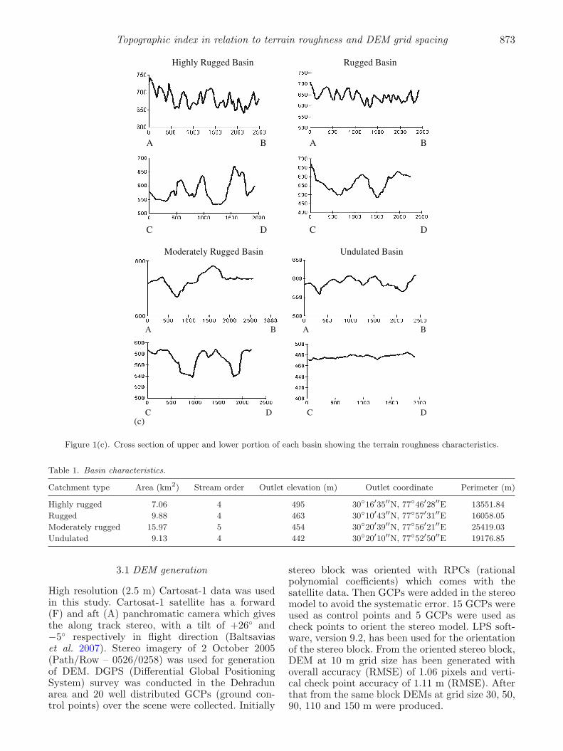
surface has also increased. Therefore, it was nec-essary to find out whether the dispersion of thetopographic index also increased with grid spac-ing or not. In order to find this, RMSE (table 6)has been computed by subtracting the mean fromeach topographic index surface (standard error).Curve of the standard error showed that the ‘dis-persion RMSE’ of the topographic index increased

Table 6. Standard error of topographic index.


Highly rugged 2.48 2.54 2.57 2.61 2.55

Rugged 2.43 2.46 2.55 2.52 2.54


Undulated 2.70 2.79 2.65 2.83 2.57


2

2.2

2.4

2.6

2.8

3

30 m 50 m 90 m 110 m 150 m

RM

SE o

f T

opog

raph

ic in

dex

Grid spacing

Highly Rugged

Rugged

Moderately Rugged

Undulated

Figure 16. Dispersion accuracy of topographic index calculated for all basins at various grid spacing.

very slowly up to 90 m grid spacing and afterthat it decreased (figure 16). This observationagain supported the finding that terrain roughnesswas a relevant terrain characteristic for the topo-graphic index accuracy and increasing mean wasthe prime deterioration factor of the topographicindex.

5. Conclusions

The present study evaluates topographic index inthe tropical climatic region considering four water-sheds with different relief characteristics, located inHimalayan terrain. The results achieved from thestatistical analysis reveal that grid spacing of DEMinfluences the calculation of topographic index.The statistics (minimum, maximum, mean andstandard deviation) of topographic index changeswhen computed from larger spacing DEMs. Repre-sentation of the ground surface is smooth in largerspacing DEM and calculation of topographic indexvalue is higher. The mean of topographic indexsurface is continuously increasing with higher gridspacing DEMs and the trend is close to linear func-tion up to 90 m grid size. The mean is higher inthe undulated basin than highly rugged and ruggedbasin because of the inverse relationship betweensurface slope and topographic index. The mean oftopographic index is highly (R2 is 0.809) correlatedwith the mean of slope which implies the influ-ence slope on the calculation of topographic index.It is also found that mean of topographic index ismore affected in the rough terrain in larger gridspacing.

The behaviour of the DEM and topographicindex is different when increasing the grid spacing.The mean of topographic index shows an increas-ing trend when calculated from coarse spacingDEMs but the mean elevation remains constantirrespective of grid size and terrain roughness. Thespatial autocorrelation of topographic index sur-face declines when computed from larger spacingDEMs. The small channels are invisible withinthe coarse grid and the pattern of the surface ischanging.

Analyzing the accuracy of the topographic index,the study found that grid spacing and terrainroughness affect the calculation of topographicindex. In the rough terrain, the accuracy of thetopographic index is violated while moving towardslarger grid spacing. RMSE of topographic indexsurface is 2.93 at 30 m grid spacing which increasesto 5.33 at 150 m grid spacing in highly ruggedbasin. But in undulated basin, the RMSE variesfrom 3.20 to 4.47 when the grid spacing is increasedfrom 30 to 150 m. Higher the grid spacing of aDEM, calculated slope is less and the topographicindex is overestimated. The overestimation of topo-graphic index is higher in the rough terrain whichis due to terrain relief. Terrain relief determines theslope as well as change of slope of any basin andthe topographic index is inversely proportional toslope. The higher value of mean error in the ruggedterrain signifies the fact.

The present study concludes that for the givensetting beyond 90 m grid spacing, the topographicindex becomes unreliable with respect to the topo-graphic index calculated from a 10 m grid spacingDEM. Since after 90 m grid spacing accuracy of


the topographic index highly deteriorates which ismore pronounced in rugged terrain.

Further investigation can be made to evaluatethe accuracy of topographic index considering thefollowing issues:

• Identification of most suitable algorithm (sin-gle flow direction or multiple flow direction) forderivation of the topographic index in a specificterrain.

• Analysis of the accuracy of topographic indexon the hydrological model outcome and theirrelationship.

• Applicability of the present study in various cli-matic regions considering more number of water-sheds.

Acknowledgements

Authors are thankful to Indian Institute of RemoteSensing, Dehradun and International Institute ofGeo-information Science and Earth Observation(ITC), The Netherlands, for providing the data andsupport for this research. Authors are also thankfulto the anonymous reviewers for their comments.

References

Baltsavias E, Kocaman S and Wolff K 2007 Geometric andradiometric investigations of Cartosat-1 data; In: ISPRSHannover Workshop 2007, High Resolution Earth Imag-ing for Geospatial Information, Hannover, Germany,May 29–June 1.

Beven K and Kirkby M J 1979 A physically based variablecontributing area model of basin hydrology; Hydrol. Sci.Bull. 24 43–69.

Brasington J and Richards K 1998 Interactions betweenmodel predictions, parameters and DTM scales for top-model; Comput. Geosci. 24(4) 299–314.

Burrough P A, Wilson J P and Gaans P F M V 2001 Fuzzyk-means classification of topo-climatic data as an aid toforest mapping in the Greater Yellowstone Area, USA;Landscape Ecol. 16 523–546.

Cai X and Wang D 2006 Spatial autocorrelation of topo-graphic index in catchments; J. Hydrol. 328 581–591.

Chappell N A, Vongtanaboon S, Jiang Y and Tangtham N2006 Return-flow prediction and buffer designation in tworainforest headwaters; Forest Ecol. Manag. 224 131–146.

Dale M R T and Fortin M J 2002 Spacial autocorrelationand statistical tests in ecology; Ecoscience 9(2) 162–167.

Demoulin A, Bovy B, Rixhon G and Cornet Y 2007 Anautomated method to extract fluvial terraces from digi-tal elevation models: The Vesdre valley, a case study ineastern Belgium; Geomorphology 91 51–64.

Dragut L and Eisank C 2011 Object representations at mul-tiple scales from digital elevation models; Geomorphology129 183–189.

Gomez-Plaza A, Martınez-Mena M, Albaladejo J andCastillo V M 2001 Factors regulating spatial distribu-tion of soil water content in small semiarid catchments;J. Hydrol. 253 211–226.

Goodchild M F 1986 Spatial Autocorrelation: Concepts andTechniques in Modern Geography ; Geo Books, Norwich,UK.

Grayson R B, Western A W, Chiew F H S and Bloschl G1997 Preferred states in spatial soil moisture patterns:Local and nonlocal controls; Water Resour. Res. 33(12)2897–2908.

Grimaldi S, Nardi F, Benedetto F, Istanbulluoglu E andBras R L 2007 A physically-based method for removingpits in digital elevation models; Adv. Water Resour. 302151–2158.

Guth P L 1995 Slope and aspect calculations on gridded dig-ital elevation models: Examples from a geomorphomet-ric toolbox for personal computers; Zeitschrift GeomorphN.F. Suppl.-Bd. 101 31–52.

Hjerdt K N, McDonnell J J, Seibert J and Rodhe A 2004 Anew topographic index to quantify downslope controls onlocal drainage; Water Resour. Res. 40(5) W05602.

Huang B and Jiang B 2002 AVTOP: A full integration ofTOPMODEL into GIS; Environ. Modelling & Software17 261–268.

Irvin B J, Ventura S J and Slater B K 1997 Fuzzy andisodata classification of landform elements from digitalterrain data in Pleasant Valley, Wisconsin; Geoderma77(2–4) 137–154.

Jenson S K and Domingue J O 1988 Extraction topographicstructure from digital elevation data for geographic infor-mation system analysis; Photogram. Eng. Rem. Sens.54(11) 1593–1600.

Joshi P K, Yadav K and Sinha V S P 2011 Assessing impactof forest landscape dynamics on migratory corridors: Acase study of two protected areas in Himalayan foothills;Biodiversity and Conservation 20(14) 3393–3411.

Kakembo V, Rowntree K and Palmer A R 2007 Topographiccontrols on the invasion of Pteronia incana (Blue bush)onto hillslopes in Ngqushwa (formerly Peddie) district,Eastern Cape, South Africa; Catena 70 185–199.

Kennelly P J 2008 Terrain maps displaying hill-shading withcurvature; Geomorphology 102 567–577.

Kumar P, Verdin K L and Greenlee S K 2000 Basinlevel statistical properties of topographic index for NorthAmerica; Adv. Water Resour. 23 571–578.

Mackey B G 1994 Predicting the potential distribution ofrain-forset structural characteristics; J. Vegetation Sci.5(1) 43–54.

Merot P, Squividant H, Aurousseau P, Hefting M, Burt T,Maitre V, Kruk M, Butturini A, Thenail C and Viaud V2003 Testing a climato-topographic index for predictingwetlands distribution along a European climate gradient;Ecological Modelling 163 51–71.

Moreno M, Levachkine S, Torres M, Quintero R andGuzman G 2005 Automatic geomorphometric analysisfor digital elevation models; Lecture Notes in ArtificialIntelligence 3684 374–381.

Nolan B T, Healy R W, Taber P E, Perkins K, Hitt KJ and Wolock D M 2007 Factors influencing ground-water recharge in the eastern United States; J. Hydrol.332(1–2) 187–205.

O’Loughlin E M 1986 Prediction of surface saturation zonesin natural catchments by topographic analysis; WaterResour. Res. 22(5) 794–804.

Pan F, Lidard C D P, Sale M J and King A W 2004A comparison of geographical information systems-basedalgorithms for computing the TOPMODEL topographicindex; Water Resour. Res. 40 1–11.

Pei T, Qin C Z, Zhu A X, Yang L, Luo M, Li B and Zhou C2010 Mapping soil organic matter using the topographicwetness index: A comparative study based on differentflow-direction algorithms and kriging methods; EcologicalIndicators 10(3) 610–619.

Peifa W, Jinkang D U, Xuezhi F and Guoding K 2006 Effectof uncertainty of grid DEM on TOPMODEL: Evaluationand analysis; Chinese Geogr. Sci. 16(4) 320–326.


Quinn P F and Beven K 1993 Spatial and temporal pre-dictions of soil moisture dynamics, runoff, variable sourceareas and evapotranspiration for Plinlimon, Mid-Wales;Hydrol. Proces. 5 59–79.

Quinn P F, Beven K, Chevallier P and Planchon O 1991 Theprediction of hillslope flow paths for distributed hydro-logical modelling using digital terrain models; Hydrol.Proces. 5 59–79.

Quinn P F, Beven K J and Lamb R 1995 The ln(a/tan b)index: How to calculate it and how to use it within theTOPMODEL framework; Hydrol. Proces. 9 161–182.

Raaflaub L D and Collins M J 2006 The effect of errorin gridded digital elevation models on the estimationof topographic parameters; Environmental Modelling &Software 21 710–732.

Saadat H, Bonnell R, Sharifi F, Mehuys G, Namdar M andAle-Ebrahim S 2008 Landform classification from a digi-tal elevation model and satellite imagery; Geomorphology100 453–464.

Schmidt F and Persson A 2003 Comparison of DEM datacapture and topographic wetness indices; Precision Agri-culture 4 179–192.

Shortridge A 2007 Practical limits of Moran’s autocorrela-tion index for raster class maps; Computers, Environmentand Urban System 31 362–371.

Si B C and Farrell R E 2004 Scale-dependent relationshipbetween wheat yield and topographic indices; Soil Sci.Soc. Am. J. 68(2) 577–587.

Tempfli K 2000 DTM accuracy assessment; In: Proceed-ings of 1999 ASPRS Annual Conference: From imageto information: Portland, Oregon, May 17–21, Bethesda:American Society for Photogrammetry and RemoteSensing (ASPRS), 11p.

Tombul M 2007 Mapping field surface soil moisture forhydrological modeling; Water Resour. Manag. 21(11)1865–1880.

Van Niel K P, Laffan S W and Lees B G 2004 Effect of errorin the DEM on environmental variables for predictivevegetation modeling; J. Veg. Sci. 15(6) 747–756.

Vaze J, Teng J and Spencer G 2010 Impact of DEM accuracyand resolution on topographic indices; EnvironmentalModelling & Software 25(10) 1086–1098.

Western A W, Grayson R B, Bloschl G, Willgoose G R andMcMahon T A 1999 Observed spatial organization of soilmoisture and its relation to terrain indices; Water Resour.Res. 35(3) 797–810.

Western A W, Zhou S L, Grayson R B, McMahon T A,Bloschl G and Wilson D J 2004 Spatial correlation of soilmoisture in small catchments and its relationship to dom-inant spatial hydrological processes; J. Hydrol. 286(1–4)113–134.

Wilson J P and Gallant J C 2000 Digital terrain analysis;In: Terrain Analysis: Principles and Applications (eds)Wilson J P and Gallant J C (New York: John Wiley &Sons), pp. 1–27.

Wimberly M C and Reilly M J 2007 Assessment of fire sever-ity and species diversity in the southern Appalachiansusing Landsat TM and ETM+ imagery; Remote Sens.Environ. 108(2) 189–197.

Wolock D M and McCabe Jr G J 1995 Comparison of sin-gle and multiple flow direction algorithms for computingtopographic parameters in TOPMODEL; Water Resour.Res. 31(5) 1315–1324.

Wolock D M and Price C V 1994 Effects of digital elevationmodel map scale and data resolution on a topography-based watershed model; Water Resour. Res. 30(11)3041–3052.

Wu S, Li J and Huang G H 2007 Modeling theeffects of elevation data resolution on the perfor-mance of topography-based watershed runoff simulation;Environmental Modelling & Software 22 1250–1260.

Wu S, Li J and Huang G H 2008 A study on DEM-derivedprimary topographic attributes for hydrological appli-cations: Sensitivity to elevation data resolution; Appl.Geogr. 28 210–223.

Yesilnacar E and Topal T 2005 Landslide susceptibility map-ping: A comparison of logistic regression and neural net-works methods in a medium scale study, Hendek region(Turkey); Eng. Geol. 79(3–4) 251–266.

Yong B, Zhang W, Niu G Y, Ren L L and Qin C Z 2009Spatial statistical properties and scale transform analyseson the topographic index derived from DEMs in China;Comput. Geosci. 35(3) 592–602.

Yue T X, Du Z P, Song D J and Gong Y 2007 A newmethod of surface modelling and its application to DEMconstruction; Geomorphology 91 161–172.

Zhang W and Montgomery D R 1994 Digital elevationmodel grid size, landscape representation, and hydrologicsimulation; Water Resour. Res. 30(4) 1019–1028.

Zinko U, Seibert J, Dynesius M and Nilsson C 2005 Plantspecies numbers predicted by a topography-based ground-water flow index; Ecosystem 8(4) 430–441.

MS received 7 May 2012; revised 7 November 2012; accepted 20 November 2012

evaluation of topographic index in relation to terrain

Documents