Evaluation of terrestrial carbon cycle models for theirresponse to climate variability and to CO2 trendsSH ILONG P IAO * † , S TEPHEN S I TCH ‡ , PH I L I PPE C IA I S § , P I ERRE FR I EDL INGSTE IN ‡ ,

PH I L I PPE PEYL IN § , XUHU I WANG * , ANDERS AHLSTR €OM ¶ , ALE S SANDRO ANAV ‡ ,

J O SEP G . CANADELL|| , NAN CONG * , CHR I S HUNT INGFORD * * , MART IN JUNG † † ,

SAM LEV I S ‡ ‡ , P ETER E . LEVY § § , J UNSHENG L I ¶ ¶ , X IN L IN¶¶ , |||| , MARK R LOMAS * * * ,MENG LU † † † , Y IQ I LUO ‡ ‡ ‡ , YUECUN MA * , RANGA B . MYNEN I § § § , B EN POULTER § ,ZHENZHONG SUN* , TAO WANG§ , NICOLAS VIOVY§ , SOENKE ZAEHLE†† and NING ZENG¶¶¶

*Sino-French Institute for Earth System Science, College of Urban and Environmental Sciences, Peking University, Beijing

100871, China, †Institute of Tibetan Plateau Research, Chinese Academy of Sciences, Beijing 100085, China, ‡College of

Engineering, Computing and Mathematics, University of Exeter, Exeter EX4 4QF, UK, §Laboratoire des Sciences du Climat et de

l’Environnement, CEA CNRS UVSQ, Gif-sur-Yvette 91191, France, ¶Department of Physical Geography and Ecosystem Science,

Lund University, Solvegatan 12, Lund SE 223 62, Sweden, ||Global Carbon Project, Commonwealth Scientific and Industrial

Research Organization, Marine and Atmospheric Research, Canberra, Australia, **Centre for Ecology and Hydrology, Benson

Lane, Wallingford, OX10 8BB, UK, ††Max Planck Institute for Biogeochemistry, P.O. Box 10 01 64, Jena 07701, Germany,

‡‡National Center for Atmospheric Research, Boulder, CO 80301, USA, §§Centre for Ecology and Hydrology, Bush Estate,

Penicuik, Midlothian EH26 0QB, UK, ¶¶State Key Laboratory of Environmental Criteria and Risk Assessment, Chinese Research

Academy of Environmental Sciences, Beijing 100012, People’s Republic of China, ||||College of Water Sciences, Beijing Normal

University, Beijing 100875, People’s Republic of China, ***Department of Animal & Plant Sciences, University of Sheffield,

Sheffield S10 2TN, UK, †††Institute of Biodiversity Science, Fudan University, 220 Handan Road, Shanghai 200433, China,

‡‡‡Department of Microbiology and Plant Biology, University of Oklahoma, Norman, OK 73019, USA, §§§Department of

Geography and Environment, Boston University, 675 Commonwealth Avenue, Boston, MA 02215, USA, ¶¶¶Department of

Atmospheric and Oceanic Science, University of Maryland, College Park, MD 20740, USA

Abstract

The purpose of this study was to evaluate 10 process-based terrestrial biosphere models that were used for the IPCC

fifth Assessment Report. The simulated gross primary productivity (GPP) is compared with flux-tower-based esti-

mates by Jung et al. [Journal of Geophysical Research 116 (2011) G00J07] (JU11). The net primary productivity (NPP)

apparent sensitivity to climate variability and atmospheric CO2 trends is diagnosed from each model output, using

statistical functions. The temperature sensitivity is compared against ecosystem field warming experiments results.

The CO2 sensitivity of NPP is compared to the results from four Free-Air CO2 Enrichment (FACE) experiments. The

simulated global net biome productivity (NBP) is compared with the residual land sink (RLS) of the global carbon

budget from Friedlingstein et al. [Nature Geoscience 3 (2010) 811] (FR10). We found that models produce a higher GPP

(133 � 15 Pg C yr�1) than JU11 (118 � 6 Pg C yr�1). In response to rising atmospheric CO2 concentration, modeled

NPP increases on average by 16% (5–20%) per 100 ppm, a slightly larger apparent sensitivity of NPP to CO2 than that

measured at the FACE experiment locations (13% per 100 ppm). Global NBP differs markedly among individual

models, although the mean value of 2.0 � 0.8 Pg C yr�1 is remarkably close to the mean value of RLS (2.1 � 1.2

Pg C yr�1). The interannual variability in modeled NBP is significantly correlated with that of RLS for the period

1980–2009. Both model-to-model and interannual variation in model GPP is larger than that in model NBP due to the

strong coupling causing a positive correlation between ecosystem respiration and GPP in the model. The average lin-

ear regression slope of global NBP vs. temperature across the 10 models is �3.0 � 1.5 Pg C yr�1 °C�1, within the

uncertainty of what derived from RLS (�3.9 � 1.1 Pg C yr�1 °C�1). However, 9 of 10 models overestimate the regres-

sion slope of NBP vs. precipitation, compared with the slope of the observed RLS vs. precipitation. With most models

lacking processes that control GPP and NBP in addition to CO2 and climate, the agreement between modeled and

observation-based GPP and NBP can be fortuitous. Carbon–nitrogen interactions (only separable in one model)

significantly influence the simulated response of carbon cycle to temperature and atmospheric CO2 concentration,

suggesting that nutrients limitations should be included in the next generation of terrestrial biosphere models.

Keywords: carbon cycle, CO2 fertilization, model evaluation, precipitation sensitivity, temperature sensitivity

Received 8 February 2013; revised version received 8 February 2013 and accepted 17 February 2013

Correspondence: Shilong Piao, e-mail: slpiao@pku.edu.cn

© 2013 Blackwell Publishing Ltd 1

Global Change Biology (2013), doi: 10.1111/gcb.12187

Introduction

The human perturbation of the carbon cycle largely

drives climate change, directly through emissions but

also via climate feedbacks on natural carbon sources

and sinks. The terrestrial carbon cycle has been modeled

to be particularly sensitive to current and future climate

and atmospheric CO2 changes, but regional patterns

and mechanisms of terrestrial carbon sources and

sinks remain uncertain (Schimel et al., 2001; Houghton,

2007). During the past decades, considerable efforts

have been made to develop process-based carbon cycle

models, as tools to understand terrestrial carbon mech-

anisms and fluxes at local, regional, continental, and

global scales (Moorcroft, 2006; Huntingford et al., 2011).

Models were applied to hindcast historical changes

(Cramer et al., 2001; Piao et al., 2009a) and to forecast

future changes (Friedlingstein et al., 2006; Sitch et al.,

2008). Carbon cycle models have been tested against

CO2 fluxes measured by eddy covariance technique at

sites around the world (Sitch et al., 2003; Krinner et al.,

2005; Jung et al., 2007; St€ockli et al., 2008; Keenan et al.,

2012; W. Wang, P. Ciais, R. Nemani, J. Canadell, S. Piao,

S. Sitch, M. White, H. Hashimoto, C. Milesi, R. Myneni,

submitted), satellite-based leaf area index (LAI) retrie-

val products (Lucht et al., 2002; Piao et al., 2006, 2008),

and observed vegetation productivity and carbon stor-

age (Randerson et al., 2009). And yet, it is difficult to

draw a clear picture of model performance and short-

comings from the current model-benchmarking litera-

ture dealing with the global terrestrial carbon cycle. The

reasons for this are several: (i) in situ high-quality mea-

surements are very sparse and short term, and often

cannot be extrapolated readily to larger spatial and tem-

poral scales; (ii) satellite measurements provide only

indirect proxies of carbon variables; (iii) atmospheric

CO2 evaluates the combination of a terrestrial carbon

model, atmospheric transport model and potentially

ocean carbon models, and therefore the results depend

on the choice of the atmospheric transport model and

its bias (Stephens et al., 2007); (iv) uncertainties associ-

ated with measurements are often not reported, which

generates type-1 error (a model is estimated to be realistic

but the benchmark measurement is not accurate

enough to say this) and type-2 error (a model is esti-

mated to be erroneous because the benchmark data

were inaccurate or not relevant); and (v) several recent

studies have documented prototype benchmark

schemes for the carbon cycle (Randerson et al., 2009;

Cadule et al., 2010; Blyth et al., 2011), however, a com-

munity-wide set of agreed benchmark tests and perfor-

mance indicators is currently still under development.

Current coupled climate–carbon models used in the

fourth and fifth Assessment Reports of the Intergovern-

mental Panel on Climate Change (IPCC) generally pro-

ject a positive feedback between global warming and

the reduction in terrestrial carbon sinks in the 21st cen-

tury (Denman et al., 2007). In some instances, and for

some regions (Tropical forest, regions with frozen vul-

nerable soil carbon stores) the positive feedbacks

become stronger over time surpassing the CO2-induced

fertilization negative feedback, making the land surface

to eventually become an overall source (Cox et al.,

2000). Characterizing climate and CO2 feedbacks on the

carbon cycle has important implications for mitigation

policies designed to stabilize greenhouse gas levels

(Matthews, 2005). The magnitude of the feedback varies

markedly among models (Friedlingstein et al., 2006).

For the SRES-A2 CO2 emission scenario, the modeled

climate–carbon cycle feedback is estimated to cause an

additional increase in CO2 content of between 20 ppmv

to 200 ppmv by 2100, which corresponds to an addi-

tional global temperature increase of 0.1 °C–1.5 °C(Friedlingstein et al., 2006). The large uncertainty in car-

bon–climate feedbacks is associated with the different

sensitivities of simulated terrestrial carbon cycle pro-

cesses to changes in climate and atmospheric CO2 (Frie-

dlingstein et al., 2006; Huntingford et al., 2009). Other

important processes, such as nutrient limitations and

land use recovery, may further affect terrestrial car-

bon–climate interactions (Arneth et al., 2010; Zaehle &

Dalmonech, 2011).

In this study, a set of 10 process-based models is

tested for their ability to predict current global carbon

fluxes (GPP, NPP, & NBP) and their apparent sensitiv-

ity to climate variability and rising atmospheric CO2

concentration. The model ensemble includes: HyLand

(Levy et al., 2004), Lund-Potsdam-Jena DGVM (Sitch

et al., 2003), ORCHIDEE (Krinner et al., 2005),

Sheffield–DGVM (Woodward et al., 1995; Woodward &

Lomas, 2004), TRIFFID (Cox, 2001), LPJ-GUESS (Smith

et al., 2001), NCAR_CLM4C (Oleson et al., 2010; Law-

rence et al., 2011), NCAR_CLM4CN (Oleson et al., 2010;

Lawrence et al., 2011), OCN (Zaehle & Friend, 2010),

and VEGAS (Zeng et al., 2005b). We compare the model

output of NBP with the RLS from Friedlingstein et al.

(2010) (hereafter FR10). For global climatological GPP

we will compare model results with the data-driven

model of GPP from Jung et al. (2011) (hereafter JU11).

The JU11 model is not a direct measurement of GPP,

but a statistical model based on the space/time interpo-

lation of flux tower observations using a model tree

ensemble (MTE) regression trained with satellite

FAPAR and gridded climate fields predictors. Finally,

ecosystem controlled warming experiments (six sites)

and Free-Air CO2 Enrichment (FACE) experiments

(four sites) are used to test the sensitivity of modeled

NPP to individual changes in temperature and CO2.

© 2013 Blackwell Publishing Ltd, Global Change Biology, doi: 10.1111/gcb.12187

2 S . PIAO et al.

Material and methods

Terrestrial carbon cycle models

The 10 carbon cycle models used in this study are briefly

described in the Table S1. All models describe surface fluxes

of CO2, water and the dynamics of water and carbon pools in

response to change in climate and atmospheric composition.

However, the formulation and number of processes primarily

responsible for carbon and water exchange differs among models.

Two simulations, S1 and S2, were performed over the

period 1860–2009. In S1, models were forced with rising atmo-

spheric CO2 concentration, while climate was held constant

(recycling climate mean and variability from the early decades

of the 20th century, e.g., 1901–1920). In S2, models were forced

with reconstructed historical climate fields and rising atmo-

spheric CO2 concentration. All models used the same forcing

files, of which historical climate fields were from CRU-NCEP v4

dataset (http://dods.extra.cea.fr/data/p529viov/cruncep/) and

global atmospheric CO2 concentration was from the combina-

tion of ice core records and atmospheric observations

(Keeling & Whorf, 2005 and update). Details of the simulation

settings are described in S. Sitch, P. Friedlingstein, N. Gruber,

S. Jones, G. Murray-Tortarolo, A. Ahlstrom, S.C. Doney,

H. Graven, C. Heinze, C. Huntingford, S. Levis, P.F. Levy,

M. Lomas, B. Poulter, N. Viovy, S. Zaehle, N. Zeng, A. Arneth,

G. Bonan, L. Bopp, J.G. Canadell, F. Chevallier, P. Ciais, R.

Ellis, M. Gloor, P. Peylin, S. Piao, C. Le Quere, B. Smith, Z.

Zhu, R. Myneni (submitted). It should be noted that land use

change was not taken into account in S1 and S2.

Data-oriented global estimation of GPP

Direct observation of Gross Primary Production (GPP) at the

global scale does not exist. Thus, we used a GPP gridded data

product from a Model Tree Ensemble (MTE) model-data

fusion scheme involving eddy covariance flux tower data, cli-

mate, and satellite FAPAR fields (Jung et al., 2011), available

during 1982–2008, to compare with modeled GPP. The MTE

statistical model employed by JU11 consists of a set of regres-

sion trees trained with local GPP estimation from eddy flux

NEE measurements with the Lasslop et al. (2010) method to

separate GPP. In addition, 29 candidate predictors were used

covering climate and biophysical variables such as vegetation

types, observed temperature, precipitation and radiation, and

satellite-derived fraction of absorbed photosynthetic active

radiation (FAPAR). The ensemble of the trained regression

trees was driven by global fields of predictor variables to

derive gridded GPP estimates (Beer et al., 2010). Uncertainty of

the GPP estimated from MTE is relatively small, at about �6

Pg C yr�1 (Jung et al., 2011). However, this does not consider

other sources of uncertainty such as measurement uncertainties

of eddy covariance fluxes, of global predictor variables as

well as sampling bias driven by unevenly distributed eddy

covariance flux sites, with many sites in temperate regions and

very few sites in the tropics. As described further below, this

dataset should also be used with extreme caution for assessment

of interannual variability of GPP.

The ‘residual’ land sink (RLS)

The RLS of anthropogenic CO2 during the period 1980–2009 is

taken from the Global Carbon Project carbon budget from

Friedlingstein et al. (2010) and Le Quere et al. (2009). It is esti-

mated as a residual of all other terms that compose the global

budget of anthropogenic CO2, as no direct global observation

of land carbon balance is available, except for the global forest

sink on decadal scale (Pan et al., 2011). The RLS is the sum of

fossil fuel, cement and land use change emissions minus the

sum of observed atmospheric CO2 growth rate and modeled

ocean sink. The CO2 emissions from fossil fuel and cement are

estimated based on statistics provided by United Nations

Energy Statistics (Boden et al., 2012), British Petroleum

statistic review of world energy (http://www.bp.com/product-

landing.do?categoryId=6929&contentId=7044622), and USGS

statistics on cement production (Van Oss, 2008). Emissions

from land use change (Houghton, 1999) are based on forest

area loss national statistics published by the United Nations

Food and Agriculture Organization and a book-keeping

model (Houghton, 2010) to convert forest area changes into

net CO2 fluxes, including legacy effects of past cohorts of

deforested areas. Atmospheric annual CO2 growth rate

is derived from the NOAA/ESRL global cooperative

air-sampling network (Conway et al., 1994). The ocean sink

of anthropogenic CO2 is calculated from the average of four

ocean carbon cycle models (Le Quere et al., 2009). It is

important to note that the net land use source estimate in

FR10 is 0.3 Pg C yr�1 lower over 2000–2009 than the previ-

ous LUC emission estimate (Le Quere et al., 2009). This

lower estimate uses the same Houghton et al. model, but

takes as input data updated information on forest area

change from FAO , TBRFA 2010, instead of the TBFRA 2005.

A lower LUC emission estimate results in a lower RLS mean

value.

Field ecosystem warming experiment

Data from a harmonized field warming experiment dataset

compiled from 124 published articles (Lu et al., 2012) were

used to evaluate model performance. To compare with

model outputs, available observations of Net Primary Pro-

duction (NPP) in experimental sites with warming only

treatments and the control experiment (no warming) were

used in this study. Six sites are located over the temperate

and boreal northern hemisphere between 30°N and 70°Nwith mean annual temperature spanning from �7 °C to

16 °C and mean annual precipitation spanning from 320 mm

to 818 mm (Table S2). The magnitude of applied warming

ranges from 1 °C to 3.5 °C among different treatments and

different sites. These levels of warming are of a magnitude

equal or higher than interannual variability in temperature,

and so complement comparison of simulations S2 and their

testing against data, where for the latter an emphasis might

be placed on anomalously warm years. It should be noted

that total NPP (both aboveground and belowground NPP)

were measured in four of the sites, whereas the other two

sites (HARS and Toolik Lake) only measured aboveground

NPP.

© 2013 Blackwell Publishing Ltd, Global Change Biology, doi: 10.1111/gcb.12187

EVALUATION OF TERRESTRIAL CARBON CYCLE MODELS 3

Free-Air Carbon Dioxide Enrichment (FACE)experiments

Free-Air Carbon Dioxide Enrichment (FACE) experiment

provides field experimental data on the response of NPP to

elevated CO2. Four FACE experiments in temperate forest

stands provide data for our evaluation (Table S3). NPP was

calculated as annual carbon increments in all plant parts plus

the major inputs to detritus, litterfall, and fine root turnover.

We used data from ORNL FACE Norby et al. (2005). But these

data are corrected and extended to 2008 (Iversen et al., 2008).

Data from young stands in the early stage of sapling develop-

ment with expanding canopies, and some plots with elevated

O3 at the ASPEN FACE were not included in the dataset, as

described by Norby et al. (2005). There were in total 21 site-

year NPP observations available for our study. Site character-

istics and experiment settings in each stand can be found in

Table S3, with a more detailed description given in Norby

et al. (2005). There are no FACE experiments for tropical

ecosystems.

Analysis

Response of carbon fluxes to climate variations. We estimate

empirically the response of GPP, NPP, and NBP to climate

variability (interannual MAT and annual precipitation) over

the last three decades using a multiple regression approach

Eqn (1):

y ¼ cintxT þ dintxpþ ð1Þε

where y is the detrended anomaly of the carbon fluxes GPP,

NPP, and NBP from the S2 simulations (i.e., simulations con-

sidering change in both climate and atmospheric CO2 con-

centration, see section ‘Terrestrial carbon cycle models’)

estimated by each model. Eqn (1) is also fitted to the data-

oriented model of GPP (JU11 GPP) and to the RLS values

from FR10. The variable xT is the detrended MAT anomaly,

and xP is the detrended annual precipitation anomaly. The

fitted regression coefficients cint and dint define the apparent

carbon flux sensitivity to interannual variations in temperature

and precipitation, and e the residual error term. Note that cint

(or dint) is the contributive effect of temperature (or precipita-

tion) variations on carbon fluxes, but not the ‘true’ sensitivi-

ties of these fluxes, given that: (i) temperature and

precipitation covary over time; and (ii) other climate drivers

discarded in Eqn (1), such as solar radiation, humidity, and

wind speed may also contribute to the variability of y. The

regression coefficients are calculated using maximum likeli-

hood estimates (MLE). The uncertainty in cint and dint is

obtained from the standard error of the corresponding

regression coefficients. Data from 1980 to 2009 were used to

quantify the response of carbon fluxes to climate variations,

except for GPP where instead the period 1982–2008 was con-

sidered to be consistent with the period covered by the JU11

data-oriented estimate. To be consistent with RLS, we first

aggregate each grid cell carbon flux into a global mean flux

(see SI) and then remove the trend using a least-squares

linear fitting method.

Response of carbon fluxes to CO2 trended over the past

30 years. Two approaches were applied to estimate the

response of carbon fluxes to CO2 (b). In the first approach, bwas estimated based on S1 simulations (i.e., the simulations

where the only driver of NPP and NBP is the increase of atmo-

spheric CO2) using Eqn (2):

b ¼ DFDCO2

ð2Þ

where, ΔF is the difference of average carbon fluxes between

the last and the first 5 years of the S1 simulation, and ΔCO2 is

the corresponding change in atmospheric CO2 concentration.

To estimate the uncertainty of b, we also calculated an ensem-

ble of b values over the study period by randomly selecting a

different year over the first and last 5-year period.

In the second approach, we used a multiple regression

approach Eqn (3) to estimate b for RLS, or for JU11 GPP, and

for each model carbon flux from simulation S2 (both climate

and CO2 change).

y ¼ bCO2 þ aTmpþ bPrcpþ cþ ð3Þε

where, y is the carbon flux of each model (NBP or GPP)

from S2, or the observed RLS from FR10, and CO2, Tmp, and

Prcp are the atmospheric CO2 concentration, MAT and annual

precipitation, respectively. b, a, b, and c are regression coeffi-

cients, and e is the residual error term. The regression coeffi-

cients are calculated using maximum likelihood estimates

(MLE). Eqn (3) attributes the time series of y to what we con-

sider as the dominant drivers of change i.e., temperature, pre-

cipitation, and CO2. However, we do recognize that changes of

other meteorological forcing might influence y as well. Those

confounding drivers are implicitly accounted for in the value

of the regression coefficients. Confounding drivers are land

use, forest demography, nitrogen deposition, solar radiation,

humidity, and wind speed, which modulate the trend of RLS

time series in addition to the assumed CO2 driver. Therefore,

the inferred value of b from Eqn (3) should be treated with

caution. In general, a and b indicate the contributive effect of

temperature (resp. precipitation) variations on the carbon

fluxes variations (Fig. S1). The period 1980–2009 is used to esti-

mate the carbon fluxes sensitivities to climate and CO2, except

for GPP where the period considered is 1982–2008.

Temperature sensitivities of vegetation productivity derived

warming experiment. For warming experiments field

measurements, the sensitivity of NPP to an applied change in

temperature (generally stepwise), is estimated as the ratio of

the relative difference between NPP in warmed minus control

plots to the applied warming magnitude. The estimated tem-

perature sensitivity at each experimental site is then compared

with the ratio of cintNPP estimated from model simulations and

with the multiple regression method Eqn (1) to the 30-year

average NPP. This ratio is hereafter called RcintNPP. The model

output is sampled at the grid point containing the experimen-

tal site. In addition, we also extract modeled sensitivities in

‘climate analogue’ grid points where the mean annual temper-

ature differs by less than 1 °C and mean annual precipitation

by less than 50 mm from the conditions at each experimental

© 2013 Blackwell Publishing Ltd, Global Change Biology, doi: 10.1111/gcb.12187

4 S . PIAO et al.

site. Only analogue grid points with the same dominant

vegetation type as observed at each experimental site are

retained, e.g., for grassland warming sites; all grid points with

grassland cover of less than 50% are excluded. As models do

not explicitly represent wetland processes, we grouped wet-

land with grasslands. Using a similar approach, we estimated

the sensitivities of NPP to rising atmospheric CO2 concentra-

tion from the FACE sites and the relative response of NPP to

CO2 (RbNPP, the ratio of bNPP estimated by Eqn (2) to the

30-year average NPP in each model).

Due to the normalization of the response of NPP to temper-

ature and/or CO2, we cannot make quantitative statements

about the nature of the model-data agreement. Both, the step-

wise nature of the experiment and the magnitude of the per-

turbation may induce nonlinear effects in the ecosystems that

cannot (and should not) be reproduced by ecosystem models

simulating the consequences of a gradual and less pronounced

perturbation over the last three decades. In particular, because

of the saturating effect of CO2 on leaf level photosynthesis, we

expect to see a larger relative effect of CO2 on photosynthesis

when evaluating the increase from 338 to 386 ppm than the

response from field experiments elevating CO2 concentration

from about 360–550 ppm.

Vegetation productivity

GPP estimation

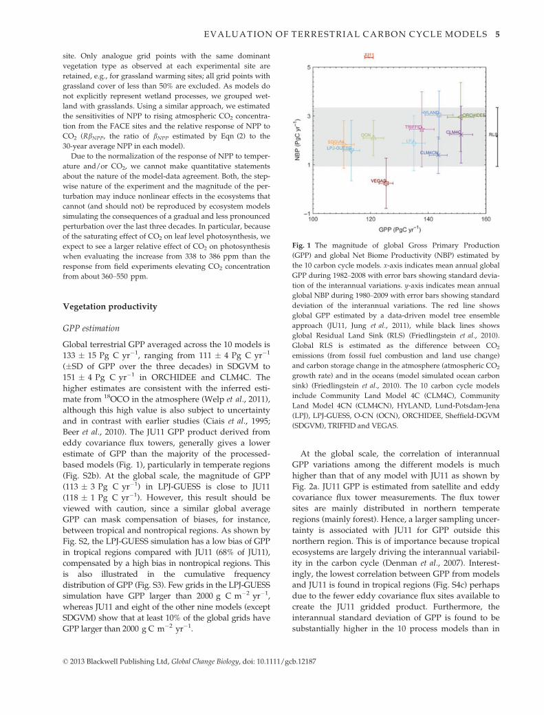
Global terrestrial GPP averaged across the 10 models is

133 � 15 Pg C yr�1, ranging from 111 � 4 Pg C yr�1

(�SD of GPP over the three decades) in SDGVM to

151 � 4 Pg C yr�1 in ORCHIDEE and CLM4C. The

higher estimates are consistent with the inferred esti-

mate from 18OCO in the atmosphere (Welp et al., 2011),

although this high value is also subject to uncertainty

and in contrast with earlier studies (Ciais et al., 1995;

Beer et al., 2010). The JU11 GPP product derived from

eddy covariance flux towers, generally gives a lower

estimate of GPP than the majority of the processed-

based models (Fig. 1), particularly in temperate regions

(Fig. S2b). At the global scale, the magnitude of GPP

(113 � 3 Pg C yr�1) in LPJ-GUESS is close to JU11

(118 � 1 Pg C yr�1). However, this result should be

viewed with caution, since a similar global average

GPP can mask compensation of biases, for instance,

between tropical and nontropical regions. As shown by

Fig. S2, the LPJ-GUESS simulation has a low bias of GPP

in tropical regions compared with JU11 (68% of JU11),

compensated by a high bias in nontropical regions. This

is also illustrated in the cumulative frequency

distribution of GPP (Fig. S3). Few grids in the LPJ-GUESS

simulation have GPP larger than 2000 g C m�2 yr�1,

whereas JU11 and eight of the other nine models (except

SDGVM) show that at least 10% of the global grids have

GPP larger than 2000 g C m�2 yr�1.

At the global scale, the correlation of interannual

GPP variations among the different models is much

higher than that of any model with JU11 as shown by

Fig. 2a. JU11 GPP is estimated from satellite and eddy

covariance flux tower measurements. The flux tower

sites are mainly distributed in northern temperate

regions (mainly forest). Hence, a larger sampling uncer-

tainty is associated with JU11 for GPP outside this

northern region. This is of importance because tropical

ecosystems are largely driving the interannual variabil-

ity in the carbon cycle (Denman et al., 2007). Interest-

ingly, the lowest correlation between GPP from models

and JU11 is found in tropical regions (Fig. S4c) perhaps

due to the fewer eddy covariance flux sites available to

create the JU11 gridded product. Furthermore, the

interannual standard deviation of GPP is found to be

substantially higher in the 10 process models than in

Fig. 1 The magnitude of global Gross Primary Production

(GPP) and global Net Biome Productivity (NBP) estimated by

the 10 carbon cycle models. x-axis indicates mean annual global

GPP during 1982–2008 with error bars showing standard devia-

tion of the interannual variations. y-axis indicates mean annual

global NBP during 1980–2009 with error bars showing standard

deviation of the interannual variations. The red line shows

global GPP estimated by a data-driven model tree ensemble

approach (JU11, Jung et al., 2011), while black lines shows

global Residual Land Sink (RLS) (Friedlingstein et al., 2010).

Global RLS is estimated as the difference between CO2

emissions (from fossil fuel combustion and land use change)

and carbon storage change in the atmosphere (atmospheric CO2

growth rate) and in the oceans (model simulated ocean carbon

sink) (Friedlingstein et al., 2010). The 10 carbon cycle models

include Community Land Model 4C (CLM4C), Community

Land Model 4CN (CLM4CN), HYLAND, Lund-Potsdam-Jena

(LPJ), LPJ-GUESS, O-CN (OCN), ORCHIDEE, Sheffield-DGVM

(SDGVM), TRIFFID and VEGAS.

© 2013 Blackwell Publishing Ltd, Global Change Biology, doi: 10.1111/gcb.12187

EVALUATION OF TERRESTRIAL CARBON CYCLE MODELS 5

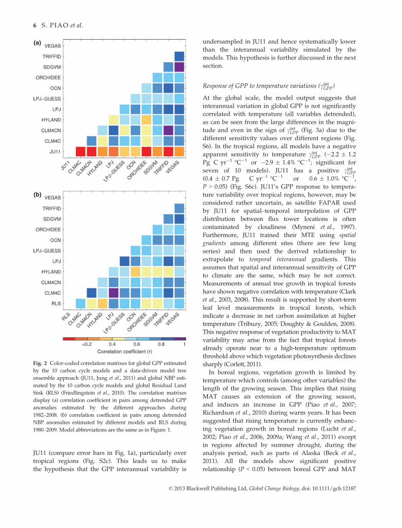
JU11 (compare error bars in Fig. 1a), particularly over

tropical regions (Fig. S2c). This leads us to make

the hypothesis that the GPP interannual variability is

undersampled in JU11 and hence systematically lower

than the interannual variability simulated by the

models. This hypothesis is further discussed in the next

section.

Response of GPP to temperature variations (cintGPP)

At the global scale, the model output suggests that

interannual variation in global GPP is not significantly

correlated with temperature (all variables detrended),

as can be seen from the large differences in the magni-

tude and even in the sign of cintGPP (Fig. 3a) due to the

different sensitivity values over different regions (Fig.

S6). In the tropical regions, all models have a negative

apparent sensitivity to temperature cintGPP (�2.2 � 1.2

Pg C yr�1 °C�1 or �2.9 � 1.4% °C�1; significant for

seven of 10 models). JU11 has a positive cintGPP

(0.4 � 0.7 Pg C yr�1 °C�1 or 0.6 � 1.0% °C�1,

P > 0.05) (Fig. S6c). JU11’s GPP response to tempera-

ture variability over tropical regions, however, may be

considered rather uncertain, as satellite FAPAR used

by JU11 for spatial–temporal interpolation of GPP

distribution between flux tower locations is often

contaminated by cloudiness (Myneni et al., 1997).

Furthermore, JU11 trained their MTE using spatial

gradients among different sites (there are few long

series) and then used the derived relationship to

extrapolate to temporal interannual gradients. This

assumes that spatial and interannual sensitivity of GPP

to climate are the same, which may be not correct.

Measurements of annual tree growth in tropical forests

have shown negative correlation with temperature (Clark

et al., 2003, 2008). This result is supported by short-term

leaf level measurements in tropical forests, which

indicate a decrease in net carbon assimilation at higher

temperature (Tribuzy, 2005; Doughty & Goulden, 2008).

This negative response of vegetation productivity to MAT

variability may arise from the fact that tropical forests

already operate near to a high-temperature optimum

threshold above which vegetation photosynthesis declines

sharply (Corlett, 2011).

In boreal regions, vegetation growth is limited by

temperature which controls (among other variables) the

length of the growing season. This implies that rising

MAT causes an extension of the growing season,

and induces an increase in GPP (Piao et al., 2007;

Richardson et al., 2010) during warm years. It has been

suggested that rising temperature is currently enhanc-

ing vegetation growth in boreal regions (Lucht et al.,

2002; Piao et al., 2006, 2009a; Wang et al., 2011) except

in regions affected by summer drought, during the

analysis period, such as parts of Alaska (Beck et al.,

2011). All the models show significant positive

relationship (P < 0.05) between boreal GPP and MAT

(a)

(b)

Fig. 2 Color-coded correlation matrixes for global GPP estimated

by the 10 carbon cycle models and a data-driven model tree

ensemble approach (JU11, Jung et al., 2011) and global NBP esti-

mated by the 10 carbon cycle models and global Residual Land

Sink (RLS) (Friedlingstein et al., 2010). The correlation matrixes

display (a) correlation coefficient in pairs among detrended GPP

anomalies estimated by the different approaches during

1982–2008. (b) correlation coefficient in pairs among detrended

NBP anomalies estimated by different models and RLS during

1980–2009. Model abbreviations are the same as in Figure 1.

© 2013 Blackwell Publishing Ltd, Global Change Biology, doi: 10.1111/gcb.12187

6 S . PIAO et al.

with an average cintGPP of 0.8 � 0.3 Pg C yr�1 °C�1 (or

4.5 � 1.5% °C�1). This apparent temperature sensitiv-

ity is close to the cintGPP diagnosed from the GPP of

JU11 (0.9 � 0.3 Pg C yr�1 °C�1 or 4.7 � 1.5% °C�1)

(Fig. S6a).

In temperate regions, the response of GPP to MAT

depends partly on the balance between the positive

effect of warming through extending the growing sea-

son in spring and possibly in autumn and the negative

effect of warming through enhanced soil moisture

stress in summer. Some recent work also suggests that

the photoperiod may limit GPP (Bauerle et al., 2012). At

the regional scale, most models (except CLM4CN and

HYLAND) and JU11 show a nonsignificant interannual

correlation between MAT and GPP (Fig. S6b).

Comparison with the field warming experiments

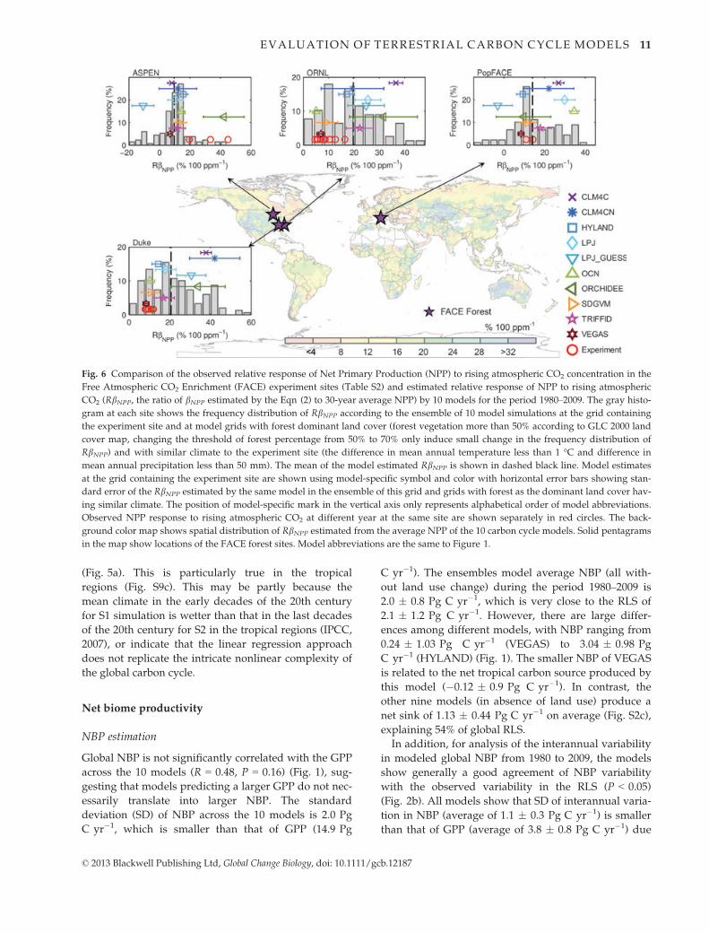
Figure 4 shows the spatial distribution of RcintNPP (the

ratio of cintNPP to the 30-year average NPP of each model)

averaged across the 10 models. Similar to the regional

scale analyses of cintGPP above, we obtained a positive

(resp. negative) interannual correlation between MAT

and NPP in boreal (resp. tropical) regions. We then

compared the simulated RcintNPP against the relative

sensitivity observed in field warming experiments (note

only distributed over the northern hemisphere). Field

warming experiments show that a step increase in tem-

perature generally increases NPP (after 4 years of

warming on average) across most sites, except at the

Haibei Alpine Research Station (in the Tibet Plateau)

where rising temperature significantly decreased

aboveground NPP by �8% °C�1 (Fig. 4). The sign of

RcintNPP at Haibei is correctly captured by six of 10 mod-

els (Fig. 4). One can also see in Fig. 4 that models tend

to predict smaller RcintNPP values than observed at the

warming experiment temperate sites, particularly at

Jasper Ridge Global Change Experiment (JRGCE),

Kessler’s Farm Field Laboratory (KFFL), Alborn (Min-

nesota 2), and Duolun. One can assume that this may

be because in the grid points containing these sites,

annual precipitation used in model forcing is less than

actual precipitation at field sites (by 15% at Jasper

Ridge Global Change Experiment, 8% at Kessler’s Farm

Field Laboratory, 46% at Toivola and Alborn, and 17%

at Duolun). The results of two field warming experi-

ment sites in Minnesota, USA (47°N, 92°W) have shown

that the wetter site (annual precipitation of 762 mm)

has a much higher NPP sensitivity to warming (12–-22% °C�1 yr�1) than the drier site (annual precipitation

of 497 mm, �3–6% °C�1 yr�1) (Fig. 4), implying that

average climatic conditions (in particular through soil

moisture availability) regulate the response of NPP to

temperature. To minimize the effect of biases in the cli-

mate drivers, we also extracted RcintNPP at ‘climate ana-

logue’ grid points where the mean annual temperature

differs by less than 1 °C and mean annual precipitation

by less than 50 mm from the conditions at each experi-

mental site. As shown in Fig. 4, however, the model

(a)

(b)

Fig. 3 The response of global Gross Primary Production (GPP),

global Net Biome Production (NBP) and global Residual Land

Sink (RLS) to (a) interannual variation in temperature (cintGPP,

cintNBP and cintRLS, respectively) and (b) interannual variation in pre-

cipitation (dintGPP, dintNBP and dintRLS, respectively). c

intGPP and dintGPP are

estimated using Eqn (1) with data during 1982–2008. cintNBP, dintNBP,

cintRLS, and dintRLS estimated using Eqn (1) with data during

1980–2009. Gray area indicates the standard error of cintRLS and

dintRLS. Error bars show standard error of the sensitivity estimates.

Dashed error bars in both (a) and (b) indicate the estimated

sensitivity from the regression approaches are statistically

insignificant (P > 0.05). The red line shows the 1r range of bGPPestimated by JU11’s GPP products using Eqn (3). Model abbre-

viations are the same as in Figure 1.

© 2013 Blackwell Publishing Ltd, Global Change Biology, doi: 10.1111/gcb.12187

EVALUATION OF TERRESTRIAL CARBON CYCLE MODELS 7

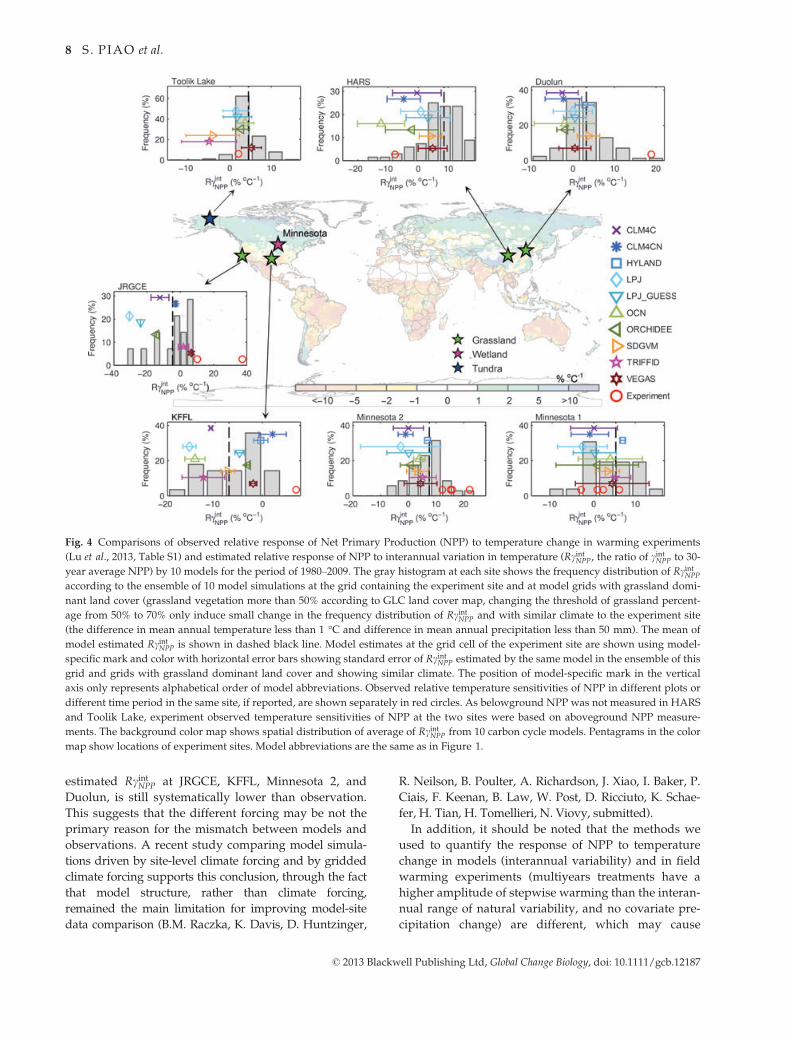
estimated RcintNPP at JRGCE, KFFL, Minnesota 2, and

Duolun, is still systematically lower than observation.

This suggests that the different forcing may be not the

primary reason for the mismatch between models and

observations. A recent study comparing model simula-

tions driven by site-level climate forcing and by gridded

climate forcing supports this conclusion, through the fact

that model structure, rather than climate forcing,

remained the main limitation for improving model-site

data comparison (B.M. Raczka, K. Davis, D. Huntzinger,

R. Neilson, B. Poulter, A. Richardson, J. Xiao, I. Baker, P.

Ciais, F. Keenan, B. Law, W. Post, D. Ricciuto, K. Schae-

fer, H. Tian, H. Tomellieri, N. Viovy, submitted).

In addition, it should be noted that the methods we

used to quantify the response of NPP to temperature

change in models (interannual variability) and in field

warming experiments (multiyears treatments have a

higher amplitude of stepwise warming than the interan-

nual range of natural variability, and no covariate pre-

cipitation change) are different, which may cause

Fig. 4 Comparisons of observed relative response of Net Primary Production (NPP) to temperature change in warming experiments

(Lu et al., 2013, Table S1) and estimated relative response of NPP to interannual variation in temperature (RcintNPP, the ratio of cintNPP to 30-

year average NPP) by 10 models for the period of 1980–2009. The gray histogram at each site shows the frequency distribution of RcintNPP

according to the ensemble of 10 model simulations at the grid containing the experiment site and at model grids with grassland domi-

nant land cover (grassland vegetation more than 50% according to GLC land cover map, changing the threshold of grassland percent-

age from 50% to 70% only induce small change in the frequency distribution of RcintNPP and with similar climate to the experiment site

(the difference in mean annual temperature less than 1 °C and difference in mean annual precipitation less than 50 mm). The mean of

model estimated RcintNPP is shown in dashed black line. Model estimates at the grid cell of the experiment site are shown using model-

specific mark and color with horizontal error bars showing standard error of RcintNPP estimated by the same model in the ensemble of this

grid and grids with grassland dominant land cover and showing similar climate. The position of model-specific mark in the vertical

axis only represents alphabetical order of model abbreviations. Observed relative temperature sensitivities of NPP in different plots or

different time period in the same site, if reported, are shown separately in red circles. As belowground NPP was not measured in HARS

and Toolik Lake, experiment observed temperature sensitivities of NPP at the two sites were based on aboveground NPP measure-

ments. The background color map shows spatial distribution of average of RcintNPP from 10 carbon cycle models. Pentagrams in the color

map show locations of experiment sites. Model abbreviations are the same as in Figure 1.

© 2013 Blackwell Publishing Ltd, Global Change Biology, doi: 10.1111/gcb.12187

8 S . PIAO et al.

inconsistencies in evaluating models. Even at the same

site, the magnitude of the temperature sensitivity of

NPP depends on the magnitude of warming. For exam-

ple, field warming experiments at the drier site in

Minnesota, USA (47°N, 92°W) show that temperature

sensitivity of NPP for a step 2 °C warming (1–6% yr�1)

is larger than that for a step 3 °Cwarming (�3–2% yr�1).

Furthermore, RcintNPP of processed-based models does not

consider local heterogeneity of environmental condi-

tions and land cover, and local biogeophysical feedbacks

with the atmosphere (e.g., Long et al., 2006). This spatial

scale mismatch adds uncertainty to model evaluation

using warming experiment sites. For instance, the tem-

perature sensitivity of NPP derived from the warming

experiment at the two Minnesota sites (47°N, 92°W) that

are located in the same grid point of models, varies from

�3% °C�1 to 22% °C�1, which is a larger range than that

predicted by the models over the corresponding grid

point (from�2.7% °C�1 to 6.1% °C�1). In addition, mod-

els may not fully represent ecosystem-level mechanisms

underlying NPP responses to warming in experiments,

such as warming-induced changes in nutrient availabil-

ity, soil moisture, phenology, and species composition

(Luo, 2007). Overall, the inconsistency of the response of

NPP to temperature change between models and field

warming experiments should be addressed by further

studies, for instance, running the same models with

site observed forcing data and vegetation, and soil

parameters.

Response of GPP to precipitation variations dintGPP

Over the past few decades, many regions experienced

drought, which has a negative effect on vegetation

productivity (Zhao & Running, 2010; for the globe;

Angert et al., 2005 and Zeng et al., 2005a for the Northern

Hemisphere; Ciais et al., 2005 for Europe; Zhang et al.,

2010 for North America; Poulter et al., 2010 for

Amazonia, Mcgrath et al., 2012; for Australia, Wang

et al., 2010 for China). Droughts that occurred from

1998 to 2002 in the northern hemisphere midlatitudes,

for example, led to an estimated reduction in vegetation

NPP by 5% compared with the average of the previous

two decades (Zeng et al., 2005a). Although individual

drought events cannot be attributed to anthropogenically

induced climate change, there is a concern that a general

situation of more extreme weather events is emerging,

including the potential for alteration to the global

hydrological cycle. Over the northern hemisphere, all

models have a positive dintGPP However, the interannual

correlation between GPP and precipitation was found

to be not significant for JU11, HYLAND, LPJ-GUESS,

and VEGAS in boreal regions (Fig. S7a), and JU11,

HYLAND in northern temperate regions (Fig. S7b).

There has been much discussion in the literature

about the impact of drought on vegetation growth and

mortality in tropical regions (Nepstad et al., 2004; Phil-

lips et al., 2009, 2010; Da Costa et al., 2010). A rainfall

exclusion experiment in an east-central Amazonian

rainforest at Tapajos showed that a 50% reduction in

precipitation led to a 25% reduction in vegetation NPP

over the first 2 years of the experiment (Nepstad et al.,

2002). It has been suggested that spatial GPP variability

in 30% of tropical forest and in 55% of tropical savann-

ahs and grasslands is primary correlated with the

precipitation (Beer et al., 2010). All models indeed show

a positive correlation of GPP with annual precipitation

over tropical regions (not significant in JU11 and

HYLAND), but the magnitude of dintGPP differs among

models with TRIFFID and LPJ having the largest dintGPP

(about 2.2 � 0.4 Pg C yr�1 per 100 mm or 2.8 � 0.5%

per 100 mm for TRIFFID, and 1.8 � 0.4 Pg C yr�1 per

100 mm or 2.7 � 0.5% per 100 mm for LPJ) (Fig. S7c).

The average of tropical dintGPP across the 10 models is

1.4 � 0.5 Pg C yr�1 per 100 mm (or 1.8 � 0.7% per

100 mm), which is three times larger than dintGPP of the

JU11 data-oriented GPP (0.5 � 0.3 Pg C yr�1 per

100 mm or 0.6 � 0.4% per 100 mm).

Overall, at the global scale, dintGPP averaged across the

10 models is 4.1 � 2.0 Pg C yr�1 per 100 mm

(or 3.1 � 1.5% per 100 mm) (Fig. 3b). Among the 10

models, eight exhibit significant positive correlations

between global GPP and annual precipitation (all vari-

ables detrended). Considering that global GPP was not

correlated with MAT in any of the models (see section

‘Response of GPP to temperature variations’), we con-

clude that interannual variation in GPP is more closely

controlled by precipitation rather than by temperature

(Piao et al., 2009b; Jung et al., 2011) in the models

parameterizations. The TRIFFID model has the highest

dintGPP (7.6 � 1.5 Pg C yr�1 per 100 mm or 5.5 � 1.1%

per 100 mm) as seen in Fig. 3b. Differences in simu-

lated land cover between models, in addition to struc-

tural sensitivities (i.e., sensitivity of stomata to soil

moisture) may also explain the variability among mod-

els, particularly in arid and temperate regions (Poulter

et al., 2011).

Response of vegetation productivity to CO2

According to the results of simulation S1 driven by

atmospheric CO2 only, model results consistently indi-

cate that rising atmospheric CO2 concentration

increased NPP by 3–10% with an average of 7% over

the past three decades (for a 48 ppm CO2 increase) (or

0.05–0.2% ppm�1 with the average of 0.16% ppm�1).

This relative response of NPP to CO2 (RbNPP) is

slightly larger than the sensitivity derived from FACE

© 2013 Blackwell Publishing Ltd, Global Change Biology, doi: 10.1111/gcb.12187

EVALUATION OF TERRESTRIAL CARBON CYCLE MODELS 9

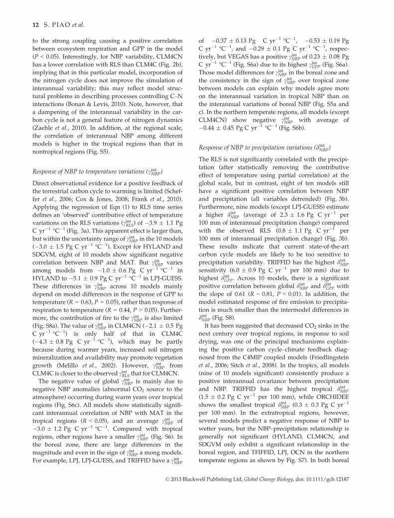
elevated CO2 experiments. This result is expected

because of the saturating effect of CO2 on photosynthe-

sis. Norby et al. (2005) analyzed the response of NPP

to elevated CO2 in four FACE experiments in temper-

ate forest stands and concluded that the enhancement

of NPP due to elevated CO2 (about 180 ppmv) was of

about 23% (or 0.13% ppm�1). When comparing the

results from the four FACE experiments with model

simulations at the corresponding sites and climatic

condition, however, we found that the models under-

estimated CO2 fertilization effect on NPP at the

ASPEN FACE site, but overestimated it at the Duke

and ORNL FACE sites (Fig. 6). The study of Hickler

et al. (2008) suggested that the currently available

FACE results are not applicable to vegetation globally

as there is large spatial heterogeneity of the positive

effect of CO2 on vegetation productivity across the

global land surface. Hence, we do not present the

FACE values in global plot Fig. 5a. As shown in Fig. 6,

the modeled response of NPP to CO2 is generally larger

in drier regions. Among the four FACE experimental

sites, a largest CO2 fertilization effect of NPP was also

found in the driest (ASPEN FACE) site (Fig. 6 and Table

S3). This NPP enhancement could be due to the

additional saving of soil moisture induced by elevated

CO2 on stomatal closure (i.e., increased water use

efficiency of plants in water limited regions).

It has been suggested that the CO2 fertilization effect

on vegetation productivity may be overestimated

because models ignore N limitations (Hungate et al.,

2003; Bonan & Levis, 2010; Zaehle et al., 2010). As in

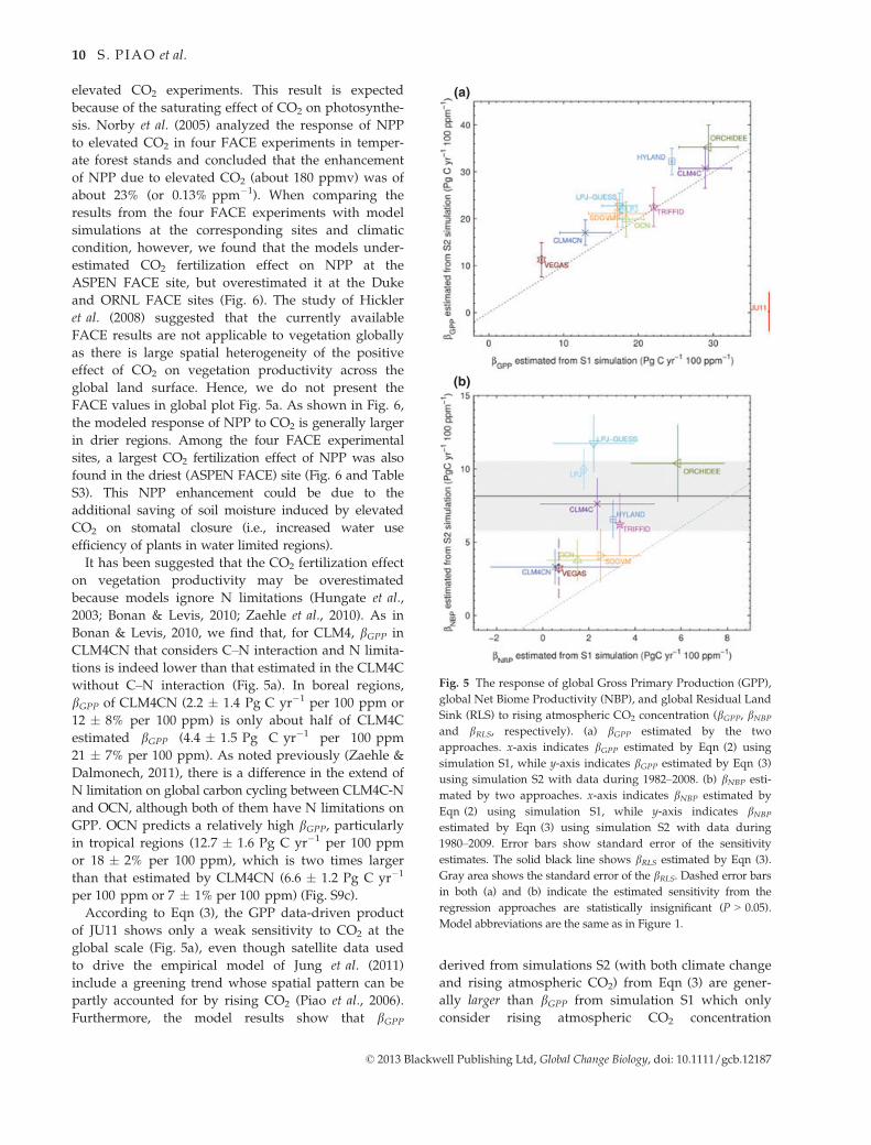
Bonan & Levis, 2010, we find that, for CLM4, bGPP in

CLM4CN that considers C–N interaction and N limita-

tions is indeed lower than that estimated in the CLM4C

without C–N interaction (Fig. 5a). In boreal regions,

bGPP of CLM4CN (2.2 � 1.4 Pg C yr�1 per 100 ppm or

12 � 8% per 100 ppm) is only about half of CLM4C

estimated bGPP (4.4 � 1.5 Pg C yr�1 per 100 ppm

21 � 7% per 100 ppm). As noted previously (Zaehle &

Dalmonech, 2011), there is a difference in the extend of

N limitation on global carbon cycling between CLM4C-N

and OCN, although both of them have N limitations on

GPP. OCN predicts a relatively high bGPP, particularlyin tropical regions (12.7 � 1.6 Pg C yr�1 per 100 ppm

or 18 � 2% per 100 ppm), which is two times larger

than that estimated by CLM4CN (6.6 � 1.2 Pg C yr�1

per 100 ppm or 7 � 1% per 100 ppm) (Fig. S9c).

According to Eqn (3), the GPP data-driven product

of JU11 shows only a weak sensitivity to CO2 at the

global scale (Fig. 5a), even though satellite data used

to drive the empirical model of Jung et al. (2011)

include a greening trend whose spatial pattern can be

partly accounted for by rising CO2 (Piao et al., 2006).

Furthermore, the model results show that bGPP

derived from simulations S2 (with both climate change

and rising atmospheric CO2) from Eqn (3) are gener-

ally larger than bGPP from simulation S1 which only

consider rising atmospheric CO2 concentration

(a)

(b)

Fig. 5 The response of global Gross Primary Production (GPP),

global Net Biome Productivity (NBP), and global Residual Land

Sink (RLS) to rising atmospheric CO2 concentration (bGPP, bNBP

and bRLS, respectively). (a) bGPP estimated by the two

approaches. x-axis indicates bGPP estimated by Eqn (2) using

simulation S1, while y-axis indicates bGPP estimated by Eqn (3)

using simulation S2 with data during 1982–2008. (b) bNBP esti-

mated by two approaches. x-axis indicates bNBP estimated by

Eqn (2) using simulation S1, while y-axis indicates bNBP

estimated by Eqn (3) using simulation S2 with data during

1980–2009. Error bars show standard error of the sensitivity

estimates. The solid black line shows bRLS estimated by Eqn (3).

Gray area shows the standard error of the bRLS. Dashed error bars

in both (a) and (b) indicate the estimated sensitivity from the

regression approaches are statistically insignificant (P > 0.05).

Model abbreviations are the same as in Figure 1.

© 2013 Blackwell Publishing Ltd, Global Change Biology, doi: 10.1111/gcb.12187

10 S . PIAO et al.

(Fig. 5a). This is particularly true in the tropical

regions (Fig. S9c). This may be partly because the

mean climate in the early decades of the 20th century

for S1 simulation is wetter than that in the last decades

of the 20th century for S2 in the tropical regions (IPCC,

2007), or indicate that the linear regression approach

does not replicate the intricate nonlinear complexity of

the global carbon cycle.

Net biome productivity

NBP estimation

Global NBP is not significantly correlated with the GPP

across the 10 models (R = 0.48, P = 0.16) (Fig. 1), sug-

gesting that models predicting a larger GPP do not nec-

essarily translate into larger NBP. The standard

deviation (SD) of NBP across the 10 models is 2.0 Pg

C yr�1, which is smaller than that of GPP (14.9 Pg

C yr�1). The ensembles model average NBP (all with-

out land use change) during the period 1980–2009 is

2.0 � 0.8 Pg C yr�1, which is very close to the RLS of

2.1 � 1.2 Pg C yr�1. However, there are large differ-

ences among different models, with NBP ranging from

0.24 � 1.03 Pg C yr�1 (VEGAS) to 3.04 � 0.98 Pg

C yr�1 (HYLAND) (Fig. 1). The smaller NBP of VEGAS

is related to the net tropical carbon source produced by

this model (�0.12 � 0.9 Pg C yr�1). In contrast, the

other nine models (in absence of land use) produce a

net sink of 1.13 � 0.44 Pg C yr�1 on average (Fig. S2c),

explaining 54% of global RLS.

In addition, for analysis of the interannual variability

in modeled global NBP from 1980 to 2009, the models

show generally a good agreement of NBP variability

with the observed variability in the RLS (P < 0.05)

(Fig. 2b). All models show that SD of interannual varia-

tion in NBP (average of 1.1 � 0.3 Pg C yr�1) is smaller

than that of GPP (average of 3.8 � 0.8 Pg C yr�1) due

Fig. 6 Comparison of the observed relative response of Net Primary Production (NPP) to rising atmospheric CO2 concentration in the

Free Atmospheric CO2 Enrichment (FACE) experiment sites (Table S2) and estimated relative response of NPP to rising atmospheric

CO2 (RbNPP, the ratio of bNPP estimated by the Eqn (2) to 30-year average NPP) by 10 models for the period 1980–2009. The gray histo-

gram at each site shows the frequency distribution of RbNPP according to the ensemble of 10 model simulations at the grid containing

the experiment site and at model grids with forest dominant land cover (forest vegetation more than 50% according to GLC 2000 land

cover map, changing the threshold of forest percentage from 50% to 70% only induce small change in the frequency distribution of

RbNPP) and with similar climate to the experiment site (the difference in mean annual temperature less than 1 °C and difference in

mean annual precipitation less than 50 mm). The mean of the model estimated RbNPP is shown in dashed black line. Model estimates

at the grid containing the experiment site are shown using model-specific symbol and color with horizontal error bars showing stan-

dard error of the RbNPP estimated by the same model in the ensemble of this grid and grids with forest as the dominant land cover hav-

ing similar climate. The position of model-specific mark in the vertical axis only represents alphabetical order of model abbreviations.

Observed NPP response to rising atmospheric CO2 at different year at the same site are shown separately in red circles. The back-

ground color map shows spatial distribution of RbNPP estimated from the average NPP of the 10 carbon cycle models. Solid pentagrams

in the map show locations of the FACE forest sites. Model abbreviations are the same to Figure 1.

© 2013 Blackwell Publishing Ltd, Global Change Biology, doi: 10.1111/gcb.12187

EVALUATION OF TERRESTRIAL CARBON CYCLE MODELS 11

to the strong coupling causing a positive correlation

between ecosystem respiration and GPP in the model

(P < 0.05). Interestingly, for NBP variability, CLM4CN

has a lower correlation with RLS than CLM4C (Fig. 2b),

implying that in this particular model, incorporation of

the nitrogen cycle does not improve the simulation of

interannual variability; this may reflect model struc-

tural problems in describing processes controlling C–Ninteractions (Bonan & Levis, 2010). Note, however, that

a dampening of the interannual variability in the car-

bon cycle is not a general feature of nitrogen dynamics

(Zaehle et al., 2010). In addition, at the regional scale,

the correlation of interannual NBP among different

models is higher in the tropical regions than that in

nontropical regions (Fig. S5).

Response of NBP to temperature variations (cintNBP)

Direct observational evidence for a positive feedback of

the terrestrial carbon cycle to warming is limited (Schef-

fer et al., 2006; Cox & Jones, 2008; Frank et al., 2010).

Applying the regression of Eqn (1) to RLS time series

defines an ‘observed’ contributive effect of temperature

variations on the RLS variations (cintRLS) of �3.9 � 1.1 Pg

C yr�1 °C�1 (Fig. 3a). This apparent effect is larger than,

but within the uncertainty range of cintNBP in the 10 models

(�3.0 � 1.5 Pg C yr�1 °C�1). Except for HYLAND and

SDGVM, eight of 10 models show significant negative

correlation between NBP and MAT. But cintNBP varies

among models from �1.0 � 0.6 Pg C yr�1 °C�1 in

HYLAND to �5.1 � 0.9 Pg C yr�1 °C�1 in LPJ-GUESS.

These differences in cintNBP across 10 models mainly

depend on model differences in the response of GPP to

temperature (R = 0.63, P = 0.05), rather than response of

respiration to temperature (R = 0.44, P > 0.05). Further-

more, the contribution of fire to the cintNBP is also limited

(Fig. S8a). The value of cintNBP in CLM4CN (�2.1 � 0.5 Pg

C yr�1 °C�1) is only half of that in CLM4C

(�4.3 � 0.8 Pg C yr�1 °C�1), which may be partly

because during warmer years, increased soil nitrogen

mineralization and availability may promote vegetation

growth (Melillo et al., 2002). However, cintNBP from

CLM4C is closer to the observed cintRLS that for CLM4CN.

The negative value of global cintNBP is mainly due to

negative NBP anomalies (abnormal CO2 source to the

atmosphere) occurring during warm years over tropical

regions (Fig. S6c). All models show statistically signifi-

cant interannual correlation of NBP with MAT in the

tropical regions (R < 0.05), and an average cintNBP of

�3.0 � 1.2 Pg C yr�1 °C�1. Compared with tropical

regions, other regions have a smaller cintNBP (Fig. S6). In

the boreal zone, there are large differences in the

magnitude and even in the sign of cintNBP a mong models.

For example, LPJ, LPJ-GUESS, and TRIFFID have a cintNBP

of �0.37 � 0.13 Pg C yr�1 °C�1, �0.53 � 0.19 Pg

C yr�1 °C�1, and �0.29 � 0.1 Pg C yr�1 °C�1, respec-

tively, but VEGAS has a positive cintNBP of 0.23 � 0.08 Pg

C yr�1 °C�1 (Fig. S6a) due to its highest cintGPP (Fig. S6a).

Those model differences for cintNBP in the boreal zone and

the consistency in the sign of cintNBP over tropical zone

between models can explain why models agree more

on the interannual variation in tropical NBP than on

the interannual variations of boreal NBP (Fig. S5a and

c). In the northern temperate regions, all models (except

CLM4CN) show negative cintNBP with average of

�0.44 � 0.45 Pg C yr�1 °C�1 (Fig. S6b).

Response of NBP to precipitation variations (dintNBP)

The RLS is not significantly correlated with the precipi-

tation (after statistically removing the contributive

effect of temperature using partial correlation) at the

global scale, but in contrast, eight of ten models still

have a significant positive correlation between NBP

and precipitation (all variables detrended) (Fig. 3b).

Furthermore, nine models (except LPJ-GUESS) estimate

a higher dintNBP (average of 2.3 � 1.6 Pg C yr�1 per

100 mm of interannual precipitation change) compared

with the observed RLS (0.8 � 1.1 Pg C yr�1 per

100 mm of interannual precipitation change) (Fig. 3b).

These results indicate that current state-of-the-art

carbon cycle models are likely to be too sensitive to

precipitation variability. TRIFFID has the highest dintNBP

sensitivity (6.0 � 0.9 Pg C yr�1 per 100 mm) due to

highest dintGPP. Across 10 models, there is a significant

positive correlation between global dintNBP and dintGPP with

the slope of 0.61 (R = 0.81, P < 0.01). In addition, the

model estimated response of fire emission to precipita-

tion is much smaller than the intermodel differences in

dintNBP (Fig. S8).

It has been suggested that decreased CO2 sinks in the

next century over tropical regions, in response to soil

drying, was one of the principal mechanisms explain-

ing the positive carbon cycle–climate feedback diag-

nosed from the C4MIP coupled models (Friedlingstein

et al., 2006; Sitch et al., 2008). In the tropics, all models

(nine of 10 models significant) consistently produce a

positive interannual covariance between precipitation

and NBP. TRIFFID has the highest tropical dintNBP

(1.5 � 0.2 Pg C yr�1 per 100 mm), while ORCHIDEE

shows the smallest tropical dintNBP (0.3 � 0.3 Pg C yr�1

per 100 mm). In the extratropical regions, however,

several models predict a negative response of NBP to

wetter years, but the NBP–precipitation relationship is

generally not significant (HYLAND, CLM4CN, and

SDGVM only exhibit a significant relationship in the

boreal region, and TFIFFID, LPJ, OCN in the northern

temperate regions as shown by Fig. S7). In both boreal

© 2013 Blackwell Publishing Ltd, Global Change Biology, doi: 10.1111/gcb.12187

12 S . PIAO et al.

and temperate regions, the highest dintNBP was also simu-

lated by the TRIFFID model due to its highest dintGPP (Fig.

S7a and b).

Response of NBP to rising atmospheric CO2

concentration (bNBP)

From the average of the 10 models, we estimated bNBP

using the simulation S1 to be 2.39 � 1.52 Pg C yr�1 per

100 ppm at the global scale. CLM4CN shows the smallest

bNBP of 0.54 � 2.79 Pg C yr�1 per 100 ppm, which is

only 23% of bNBP in CLM4C. This shows that modeling

nutrient limitation decreases the NBP sensitivity to

atmosphere CO2 concentration (Sokolov et al., 2008;

Thornton et al., 2009; Zaehle et al., 2010). ORCHIDEE

has the largest bNBP of 5.86 � 2.02 Pg C yr�1 per

100 ppm (Fig. 5b), probably due to its highest bGPPcompared with other models (Fig. 5a). Indeed, there is a

significant correlation between bNBP and bGPP across 10

models (P < 0.05), suggesting that models have different

bNBP partly because of the different CO2 fertilization

effect on the vegetation growth (Ciais et al., 2005).

Among the 10 models, CLM4CN simulates the lowest

carbon sequestration efficiency under rising atmospheric

CO2 concentration (4%), defined as the ratio of bNBP to

bGPP, whereas ORCHIDEE has the highest carbon

sequestration efficiency under rising atmospheric CO2

concentration (20%). The ratio of bNBP to bGPP for the

ensemble model average is about 12 � 4%.

Similar to bGPP (Fig. 5a), bNBP derived from simula-

tion S2 and Eqn (3) is generally larger than bNBP from

simulation S1 (Fig. 5b), particularly in tropical regions

(Fig. S10c). As shown in Fig. 5b, CLM4CN, OCN,

SDGVM, and VEGAS estimated global bNBP from the

simulation S2 with Eqn (3) are smaller than the diag-

nosed sensitivity of RLS to atmospheric CO2 (bRLS,8.12 � 2.38 Pg C yr�1 per 100 ppm) based on Eqn (3).

However, it should be noted that since other factors

such as ecosystem management and nitrogen deposi-

tion could also explain the trend of RLS over the last

three decades (Zaehle et al., 2006; Magnani et al., 2007;

Ciais et al., 2008; Bellassen et al., 2010; Zaehle &

Dalmonech, 2011), the sensitivity of RLS to CO2 from

the Eqn (3) may be overestimated.

From model testing to directions for future research

To overcome the inevitable spread of curves resulting

from a comparison of complex models with available

observations, we investigated in this study the contributive

response of models to climate variability, and compared

the modeled response to the response diagnosed from

available ‘observations’ (in fact other data-driven

models). The main contributive responses to interannu-

al climate drivers are c – the response to temperature

anomalies in units of Pg C yr�1 °C�1, d – the response

to rainfall anomalies in units of Pg C yr�1 100 mm�1,

and b – the response to CO2 trend, in units of Pg C yr�1

100 ppm�1. Four key datasets are used to estimate

these contributive responses, a data-oriented gridded

GPP field (JU11), imposed warming experiments,

imposed raised atmospheric CO2 experiments (FACE)

and the global residual land sink modeled to close the

anthropogenic CO2 budget (RLS). These four datasets

provide information on different contributive

responses, JU11 constrains c, d, and b of GPP, experi-

mental warming site data constrain c of NPP, the

(scarce) FACE site data constrain b of NPP, and the

RLS over 30 years constrains c, d, and b of NBP. We

report the following new findings.

1 The 10 carbon cycle models give a higher mean GPP

and a higher year-to-year GPP variability than the

data-driven model of JU11, particularly in tropical

regions. In tropical regions, the GPP interannual vari-

ance in JU11 can be considered too uncertain to be

useable to falsify the process models. JU11 trained

their MTE using spatial gradients among different sites

(there are few long series) and extrapolated temporal

gradients, confounding spatial and interannual sensi-

tivity of GPP to climate. To overcome this limitations

of comparing the uncertain process models with

another uncertain data-driven model, we recommend

future work to model at the site scale in which the

measurements are made (in particular the long-term

FLUXNET sites) to investigate their response to

climate drivers for different time scales, and different

ecosystems (Schwalm et al., 2010). This will also

require better protocols with site history to account

for site specific disequilibrium of biomass and soil

carbon pools (Carvalhais et al. 2008).

2 The process models generally capture the interannual

variation in the observed residual land carbon sink

(RLS) estimation over the last three decades. But the

models’ contributive response to precipitation is too

high, particularly in tropical forests and savannas

(W. Wang, P. Ciais, R. Nemani, J. Canadell, S. Piao, S.

Sitch, M. White, H. Hashimoto, C. Milesi, R. Myneni,

submitted). It is not clear, however, if this too high

contributive response of NBP to rainfall is induced

by a bias of GPP or ecosystem respiration to soil

moisture, or to an inaccurate representation of soil

moisture by models. We recommend future work to

compare the contributive response of net and gross

CO2 fluxes between models with independent large-

scale flux estimations, such as from data-driven up-

scaling of fluxes and top down inversions.

© 2013 Blackwell Publishing Ltd, Global Change Biology, doi: 10.1111/gcb.12187

EVALUATION OF TERRESTRIAL CARBON CYCLE MODELS 13

3 In response to interannual variation in temperature,

all the models are found to simulate a stronger nega-

tive response of NBP than GPP, implying that respi-

ration responds positively to temperature. To

investigate this effect, we evaluated for the first time

the global process models against site data from a

collection of ecosystem warming experiments. We

find that models tend to underpredict the response of

NPP to temperature change at the temperate sites.

However, it is difficult to tell from the warming

experiments for NPP, which have significant

between-site variation, whether this results predomi-

nantly from plant or soil respiration, or possibly both,

where the balance varies strongly depending on geo-

graphical variation. The different approaches to

derive the NPP response to temperature between

global models forced offline by gridded climate data,

and local field warming experiments that are coupled

to the atmosphere, bias as well as the fact that

process models do not consider subgrid scale hetero-

geneity in environmental conditions and vegetation

distribution. We recommend to design a global

benchmarking of carbon cycle models against ecosys-

tem warming and drought experiments, and to com-

pile a database of experiments results and forcing

data that would be open access.

4 Despite the fact that carbon cyclemodels are often sus-

pected to overestimate CO2 fertilization as a driver of

net land uptake, we found that the ensemble mean

global NPP enhancement is comparable with FACE

experiments observation. The CLM4CN model that

have nitrogen limitations do show a sensitivity of NPP

to CO2 that is 50% lower than the same models

versions (CLM4C) but without nitrogen. The strength

of the CO2 fertilization on the NBP is poorly quantified.

The magnitude of NBP response to CO2 is not merely

dependent on the NPP response. NPP increases could

create higher litterfall enhancing soil carbon stores also

available to respire. We recommend all carbon cycle

models should include nutrients, and pursue the

evaluation of C–N interactions using both global and

local observations (e.g., Zaehle et al., 2010).

Overall, reducing these uncertainties of climate sensi-

tivities of carbon fluxes is essential to more accurately

predict future dynamics of the global carbon cycle and

its feedbacks to climate system. This remains as a high

priority for the carbon cycle modeling community. We

recommend carbon cycle models to be run both ‘free

running’ with their default parameters values used in

global simulations, and ‘adjusted’ with parameters

calibrated or optimized against site observations (e.g.,

warming, precipitation, and elevated CO2 experiments,

fluxnet data) so that the ‘portability’ of improvements

gained from small scale can be assessed at larger,

regional, or global scale.

Acknowledgements

This study is part of the Regional Carbon Cycle Assessment andProcesses (RECCAP), Global Carbon Project. We thank Dr. Lawand three anonymous referees for the detailed and constructivecomments. This work was supported by the National NaturalScience Foundation of China (grant 41125004), National BasicResearch Program of China (Grant No. 2010CB950601 and2013CB956303), Foundation for Sino-EU research cooperation ofMinistry of Science and Technology of China (1003), andCARBONES EU FP7 Foundation (242316). JGC is supported bythe Australian Climate Change Science Program.

References

Angert A, Biraud S, Bonfils C et al. (2005) Drier summers cancel out the CO2 uptake

enhancement induced by warmer springs. Proceedings of the National Academy of

Sciences of the United States of America, 102, 10823–10827.

Arneth A, Harrison SP, Zaehle S et al. (2010) Terrestrial biogeochemical feedbacks in

the climate system. Nature Geosciences, 3, 525–532.

Bauerle WL, Oren R, Way DA et al. (2012) Photoperiodic regulation of the seasonal

pattern of photosynthetic capacity and the implications for carbon cycling. Proceed-

ings of the National Academy of Sciences of the United States of America, 109, 8612–8617.

Beck PS, Juday GP, Alix C et al. (2011) Changes in forest productivity across Alaska

consistent with biome shift. Ecology Letters, 14, 373–379.

Beer C, Reichstein M, Tomelleri E et al. (2010) Terrestrial gross carbon dioxide uptake:

global distribution and covariation with climate. Science, 329, 834–838.

Bellassen V, Le Maire G, Dhote JF, Ciais P, Viovy N (2010) Modelling forest manage-

ment within a global vegetation model Part 1: model structure and general behav-

iour. Ecological Modelling, 221, 2458–2474.

Blyth E, Clark DB, Ellis R et al. (2011) A comprehensive set of benchmark tests for a

land surface model of simultaneous fluxes of water and carbon at both the global

and seasonal scale. Geoscientific Model Development, 4, 255–269.

Boden, TA, Marland G, Andres RJ (2012) Global, Regional, and National Fossil-Fuel CO2

Emissions. Carbon Dioxide Information Analysis Center, Oak Ridge National Labo-

ratory, U.S. Department of Energy, Oak Ridge, TN, USA. doi: 10.3334/CDIAC/

00001_V2012

Bonan GB, Levis S (2010) Quantifying carbon-nitrogen feedbacks in the Community

Land Model (CLM4). Geophysical Research Letters, 37, L07401. doi: 10.1029/

2010gl042430

Cadule P, Friedlingstein P, Bopp L et al. (2010) Benchmarking coupled climate-carbon

models against long-term atmospheric CO2 measurements. Global Biogeochemical

Cycles, 24, GB2016. doi: 10.1029/2009gb003556

Carvalhais N, Reichstein M, Seixas J et al. (2008) Implications of the carbon cycle

steady state assumption for biogeochemical modeling performance and inverse

parameter retrieval. Global Biogeochemical Cycles, 22, GB2007. doi: 10.1029/

2007GB003033

Ciais P, Tans PP, Trolier M, White JWC, Francey RJ (1995) A Large Northern Hemi-

sphere Terrestrial CO2 Sink Indicated by the 13C/12C Ratio of Atmospheric CO2.

Science, 269, 1098–1102.

Ciais P, Reichstein M, Viovy N et al. (2005) Europe-wide reduction in primary pro-

ductivity caused by the heat and drought in 2003. Nature, 437, 529–533.

Ciais P, Schelhaas MJ, Zaehle S et al. (2008) Carbon accumulation in European forests.

Nature Geoscience, 1, 425–429.

Clark DA, Piper SC, Keeling CD, Clark DB (2003) Tropical rain forest tree growth and

atmospheric carbon dynamics linked to interannual temperature variation during

1984–2000. Proceedings of the National Academy of Sciences, 100, 5852–5857.

Clark DB, Olivas PC, Oberbauer SF, Clark DA, Ryan MG (2008) First direct land-

scape-scale measurement of tropical rain forest Leaf Area Index, a key driver of

global primary productivity. Ecology Letters, 11, 163–172.

Conway TJ, Tans PP, Waterman LS, Thoning KW, Kitzis DR, Masarie KA, Zhang N

(1994) Evidence for interannual variability of the carbon cycle from the National

Oceanic and Atmospheric Administration/Climate Monitoring and Diagnostics

Laboratory Global Air Sampling Network. Journal Of Geophysical Research, 99,

22831–22855.

© 2013 Blackwell Publishing Ltd, Global Change Biology, doi: 10.1111/gcb.12187

14 S . PIAO et al.

Corlett RT (2011) Impacts of warming on tropical lowland rainforests. Trends in Ecol-

ogy & Evolution, 26, 606–613.

Cox PM (2001) Description of the TRIFFID dynamic global vegetation model. Techni-

cal Note 24 HadleyCentre, Met Office.

Cox P, Jones C (2008) Illuminating the modern dance of climate and CO2. Science, 321,

1642–1644.

Cox PM, Betts RA, Jones CD, Spall SA, Totterdell IJ (2000) Acceleration of global warm-

ing due to carbon-cycle feedbacks in a coupled climate model. Nature, 408, 184–187.

Cramer W, Bondeau A, Woodward FI et al. (2001) Global response of terrestrial eco-

system structure and function to CO2 and climate change: results from six

dynamic global vegetation models. Global Change Biology, 7, 357–373.

Da Costa ACL, Galbraith D, Almeida S et al. (2010) Effect of 7 yr of experimental

drought on vegetation dynamics and biomass storage of an eastern Amazonian

rainforest. New Phytologist, 187, 579–591.

Doughty CE, Goulden ML (2008) Are tropical forests near a high temperature thresh-

old? Journal of Geophysical Research: Biogeosciences, 113, G00B07. doi: 10.1029/

2007JG000632

Denman K, Brasseur G, Chidthaisong A et al. (2007) “Couplings Between Changes in the

Climate System and Biogeochemistry” in Climate Change 2007: The Physical Science

Basis, Contribution of Working Group I to the Fourth Assessment Report of the Intergov-

ernmental Panel on Climate Change. Cambridge University Press, Cambridge, Uni-

ted Kingdom and United States.

Frank DC, Esper J, Raible CC, Buntgen U, Trouet V, Stocker B, Joos F (2010) Ensemble

reconstruction constraints on the global carbon cycle sensitivity to climate. Nature,

463, 527–530.

Friedlingstein P, Cox P, Betts R et al. (2006) Climate-carbon cycle feedback analysis:

results from the (CMIP)-M-4 model intercomparison. Journal of Climate, 19,

3337–3353.

Friedlingstein P, Houghton RA, Marland G et al. (2010) Update on CO2 emissions.

Nature Geoscience, 3, 811–812.

Hickler T, Smith B, Prentice IC, Mj€ofors K, Miller P, Arneth A, Sykes MT (2008) CO2

fertilization in temperate FACE experiments not representative of boreal and trop-

ical forests. Global Change Biology, 14, 1531–1542.

Houghton RA (1999) The annual net flux of carbon to the atmosphere from changes

in land use 1850–1990. Tellus Series B-chemical And Physical Meteorology, 51,

298–313.

Houghton RA (2007) Balancing the global carbon budget. Annual Review Of Earth And

Planetary Sciences, 35, 313–347.

Houghton RA (2010) How well do we know the flux of CO2 from land-use change?

Tellus Series B-Chemical And Physical Meteorology, 62, 337–351.

Hungate BA, Dukes JS, Shaw MR, Luo YQ, Field CB (2003) Nitrogen and climate

change. Science, 302, 1512–1513.

Huntingford C, Lowe JA, Booth BBB, Jones CD, Harris GR, Gohar LK, Meir P (2009)

Contributions of carbon cycle uncertainty to future climate projection spread. Tel-

lus Series B-Chemical And Physical Meteorology, 61, 355–360.

Huntingford C, Cox PM, Mercado LM, Sitch S, Bellouin N, Boucher O, Gedney N

(2011) Highly contrasting effects of different climate forcing agents on terrestrial

ecosystem services. Philosophical Transactions of the Royal Society A-Mathematical,

Physical and Engineering Sciences, 369, 2026–2037.

IPCC (2007) The Physical Science Basis: Summary for Policymakers. Intergovernment

Panel on Climate Change Secretariat, Geneva.

Iversen CM, Ledford J, Norby RJ (2008) CO2 enrichment increases carbon and nitro-

gen input from fine roots in a deciduous forest. New Phytologist, 179, 837–847.

Jung M, Le Maire G, Zaehle S et al. (2007) Assessing the ability of three land ecosys-

tem models to simulate gross carbon uptake of forests from boreal to Mediterra-

nean climate in Europe. Biogeosciences, 4, 647–656.

Jung M, Reichstein M, Margolis HA et al. (2011) Global patterns of land-atmosphere

fluxes of carbon dioxide, latent heat, and sensible heat derived from eddy covari-

ance, satellite, and meteorological observations. Journal Of Geophysical Research,

116, G00J07. doi: 10.1029/2010jg001566

Keeling CD, Whorf TP (2005) Atmospheric CO2 records from sites in the SIO sam-

pling network. In: Trends: A Compendium of Data on Global Change. Carbon Dioxide

Information Analysis Center, Oak Ridge National Laboratory, US Department of

Energy, Oak Ridge, TN, USA. http://cdiac.ornl.gov/trends/co2/sio-mlo.htm

Keenan TF, Davidson E, Moffat AM, Munger W, Richardson AD (2012) Using

model-data fusion to interpret past trends, and quantify uncertainties in future

projections, of terrestrial ecosystem carbon cycling. Global Change Biology, 18,

2555–2569.

Krinner G, Viovy N, De Noblet-Ducoudr�e N et al. (2005) A dynamic global vegetation

model for studies of the coupled atmosphere-biosphere system. Global Biogeochemi-

cal Cycles, 19, GB1015. doi: 10.1029/2003gb002199

Lasslop G, Reichstein M, Papale D et al. (2010) Separation of net ecosystem exchange

into assimilation and respiration using a light response curve approach: critical

issues and global evaluation. Global Change Biology, 16, 187–208.

Lawrence D, Oleson KW, Flanner MG et al. (2011) Parameterization improvements

and functional and structural advances in version 4 of the community land model.

Journal of Advances in Modeling Earth Systems, 3. doi: 10.1029/2011ms000045

Le Quere C, Raupach MR, Canadell JG et al. (2009) Trends in the sources and sinks of

carbon dioxide. Nature Geoscience, 2, 831–836.

Levy PE, Cannell MGR, Friend AD (2004) Modelling the impact of future changes in

climate, CO2 concentration and land use on natural ecosystems and the terrestrial

carbon sink. Global Environmental Change, 14, 21–30.

Long SP, Ainsworth EA, Leakey ADB, N€osberger J, Ort DR (2006) Food for thought:

lower-than-expected crop yield stimulation with rising CO2 concentrations. Sci-

ence, 312, 1918–1921.

Lu M, Zhou X, Luo Y et al. (2013) Responses of ecosystem carbon cycle to experimen-

tal warming: a meta-analysis. Ecology. doi: 10.1890/12-0279.1

Lucht W, Prentice IC, Myneni RB et al. (2002) Climatic control of the high-latitude

vegetation greening trend and Pinatubo effect. Science, 296, 1687–1689.

Luo Y (2007) Terrestrial carbon–cycle feedback to climate warming. Annual Review of

Ecology, Evolution, and Systematics, 38, 683–712.

Magnani F, Mencuccini M, Borghetti M et al. (2007) The human footprint in the car-

bon cycle of temperate and boreal forests. Nature, 447, 848–850.

Matthews HD (2005) Decrease of emissions required to stabilize atmospheric CO2

due to positive carbon cycle-climate feedbacks. Geophysical Research Letters, 32,

L21707. doi: 10.1029/2005GL023435

Mcgrath GS, Sadler R, Fleming K, Tregoning P, Hinz C, Veneklaas EJ (2012) Tropical

cyclones and the ecohydrology of Australia’s recent continental-scale drought.

Geophysical Research Letters, 39, L03404. doi: 10.1029/2011gl050263

Melillo JM, Steudler PA, Aber JD et al. (2002) Soil warming and carbon-cycle feed-

backs to the climate system. Science, 298, 2173–2176.

Moorcroft PR (2006) How close are we to a predictive science of the biosphere? Trends

in Ecology & Evolution, 21, 400–407.

Myneni RB, Keeling CD, Tucker CJ, Asrar G, Nemani RR (1997) Increased plant

growth in the northern high latitudes from 1981 to 1991. Nature, 386, 698–702.

Nepstad DC, Moutinho P, Dias-Filho MB et al. (2002) The effects of partial throughfall

exclusion on canopy processes, aboveground production, and biogeochemistry of

an Amazon forest. Journal Of Geophysical Research, 107, 8085. doi: 10.1029/

2001jd000360

Nepstad D, Lefebvre P, Lopes Da Silva U et al. (2004) Amazon drought and its impli-

cations for forest flammability and tree growth: a basin-wide analysis. Global

Change Biology, 10, 704–717.

Norby RJ, Delucia EH, Gielen B et al. (2005) Forest response to elevated CO2 is con-

served across a broad range of productivity. Proceedings of the National Academy of

Sciences of the United States of America, 102, 18052–18056.

Oleson KW, Lawrence DM, Gordon B et al. (2010) Technical description of version 4.0 of

the Community Land Model (CLM). NCAR/TN-478+STR. NCAR, Boulder, USA.

Pan Y, Birdsey RA, Fang J et al. (2011) A Large and Persistent Carbon Sink in the

World’s Forests. Science, 333, 988–993.

Phillips OL, Aragao LEOC, Lewis SL et al. (2009) Drought Sensitivity of the Amazon

Rainforest. Science, 323, 1344–1347.

Phillips OL, Van Der Heijden G, Lewis SL et al. (2010) Drought–mortality relation-

ships for tropical forests. New Phytologist, 187, 631–646.

Piao S, Friedlingstein P, Ciais P, Zhou L, Chen A (2006) Effect of climate and CO2

changes on the greening of the Northern Hemisphere over the past two decades.

Geophysical Research Letters, 33, L23402. doi: 10.1029/2006gl028205

Piao SL, Friedlingstein P, Ciais P, Viovy N, Demarty J (2007) Growing season extension

and its impact on terrestrial carbon cycle in the Northern Hemisphere over the past

2 decades.Global Biogeochemical Cycles, 21, 49–53. doi: 10.1029/2006gb002888

Piao SL, Ciais P, Friedlingstein P et al. (2008) Net carbon dioxide losses of northern

ecosystems in response to autumn warming. Nature, 451, 49–53.

Piao S, Ciais P, Friedlingstein P, De Noblet-Ducoudr�e N, Cadule P, Viovy N, Wang T

(2009a) Spatiotemporal patterns of terrestrial carbon cycle during the 20th century.

Global Biogeochemical Cycles, 23, GB4026. doi: 10.1029/2008gb003339

Piao S, Friedlingstein P, Ciais P, Peylin P, Zhu B, Reichstein M (2009b) Footprint of

temperature changes in the temperate and boreal forest carbon balance. Geophysi-

cal Research Letters, 36, L07404. doi: 10.1029/2009gl037381

Poulter B, Arag~ao L, Heyder U et al. (2010) Net biome production of the Amazon

Basin in the 21st century. Global Change Biology, 16, 2062–2075.

Poulter B, Frank DC, Hodson EL, Zimmermann NE (2011) Impacts of land cover and

climate data selection on understanding terrestrial carbon dynamics and the CO2

airborne fraction. Biogeosciences, 8, 2027–2036.

© 2013 Blackwell Publishing Ltd, Global Change Biology, doi: 10.1111/gcb.12187

EVALUATION OF TERRESTRIAL CARBON CYCLE MODELS 15

Randerson JT, Hoffman FM, Thornton PE et al. (2009) Systematic assessment of ter-

restrial biogeochemistry in coupled climate–carbon models. Global Change Biology,

15, 2462–2484.

Richardson AD, Andy Black T, Ciais P et al. (2010) Influence of spring and autumn

phenological transitions on forest ecosystem productivity. Philosophical Transac-

tions of the Royal Society B-Biological Sciences, 365, 3227–3246.

Scheffer M, Brovkin V, Cox PM (2006) Positive feedback between global warming

and atmospheric CO2 concentration inferred from past climate change. Geophysical

Research Letters, 33, L10702. doi: 10.1029/2005gl025044

Schimel DS, House JI, Hibbard KA et al. (2001) Recent patterns and mechanisms of

carbon exchange by terrestrial ecosystems. Nature, 414, 169–172.

Schwalm CR, Williams CA, Schaefer K et al. (2010) A model-data intercomparison of

CO2 exchange across North America: results from the North American Carbon

Program site synthesis. Journal of Geophysical Research, 115, G00H05. doi: 10.1029/

2009JG001229

Sitch S, Smith B, Prentice IC et al. (2003) Evaluation of ecosystem dynamics, plant

geography and terrestrial carbon cycling in the LPJ dynamic global vegetation

model. Global Change Biology, 9, 161–185.

Sitch S, Huntingford C, Gedney N et al. (2008) Evaluation of the terrestrial carbon

cycle, future plant geography and climate-carbon cycle feedbacks using five

Dynamic Global Vegetation Models (DGVMs). Global Change Biology, 14,

2015–2039.

Smith B, Prentice IC, Sykes MT (2001) Representation of vegetation dynamics in the

modelling of terrestrial ecosystems: comparing two contrasting approaches within

European climate space. Global Ecology And Biogeography, 10, 621–637.

Sokolov AP, Kicklighter DW, Melillo JM, Felzer BS, Schlosser CA, Cronin TW (2008)

Consequences of considering carbon–nitrogen interactions on the feedbacks

between climate and the terrestrial carbon cycle. Journal Of Climate, 21, 3776–3796.

Stephens BB, Gurney KR, Tans PP et al. (2007) Weak northern and strong tropical

land carbon uptake from vertical profiles of atmospheric CO2. Science, 316,

1732–1735.

St€ockli R, Lawrence DM, Niu GY et al. (2008) Use of FLUXNET in the Community

Land Model development. Journal Of Geophysical Research, 113, G01025. doi: 10.

1029/2007jg000562

Thornton PE, Doney SC, Lindsay K et al. (2009) Carbon-nitrogen interactions regulate

climate-carbon cycle feedbacks: results from an atmosphere-ocean general circula-

tion model. Biogeosciences, 6, 2099–2120.

Tribuzy ES (2005) Variacoes da temperatura foliar do dossel e o seuefeito na taxa as-

similatoria de CO2 na Amazonia Central, Ph.D. dissertation. Univ. de Sao Paulo,

Sao Paulo.

Van Oss HG (2008) 2006 Minerals Yearbook 16.1–16.36. US Geological Survey.

Wang W, Wang W-J, Li J-S, Wu H, Xu C, Liu T (2010) The Impact of Sustained

Drought on Vegetation Ecosystem in Southwest China Based on Remote Sensing.

Procedia Environmental Sciences, 2, 1679–1691.

Wang X, Piao S, Ciais P, Li J, Friedlingstein P, Koven C, Chen A (2011) Spring temper-

ature change and its implication in the change of vegetation growth in North

America from 1982 to 2006. Proceedings of the National Academy of Sciences, 108,

1240–1245.

Welp LR, Keeling RF, HaJ Meijer et al. (2011) Interannual variability in the oxygen

isotopes of atmospheric CO2 driven by El Nino. Nature, 477, 579–582.

Woodward FI, Lomas MR (2004) Simulating vegetation processes along the Kalahari

transect. Global Change Biology, 10, 383–392.

Woodward FI, Smith TM, Emanuel WR (1995) A global land primary productivity

and phytogeography model. Global Biogeochemical Cycles, 9, 471–490.

Van Oss HG (2008) 2006 Minerals Yearbook 16.1–16.36. US Geological Survey.

Zaehle S, Dalmonech D (2011) Carbon–nitrogen interactions on land at global scales:

current understanding in modelling climate biosphere feedbacks. Current Opinion

in Environmental Sustainability, 3, 311–320.

Zaehle S, Friend AD, Friedlingstein P, Dentener F, Peylin P, Schulz M (2010) Carbon

and nitrogen cycle dynamics in the O-CN land surface model: 2. Role of the nitro-

gen cycle in the historical terrestrial carbon balance. Global Biogeochemical Cycles,

24, GB1006. doi: 10.1029/2009GB003522

Zaehle S, Friend AD (2010) Carbon and nitrogen cycle dynamics in the O-CN land

surface model: 1. Model description, site-scale evaluation, and sensitivity to

parameter estimates. Global Biogeochemical Cycles, 24, GB1005. doi: 10.1029/

2009gb003521

Zaehle S, Sitch S, Prentice IC et al. (2006) The importance of age-related decline in for-

est npp for modeling regional carbon balances. Ecological Applications, 16,

1555–1574.

Zeng N, Mariotti A, Wetzel P (2005a) Terrestrial mechanisms of interannual CO2 vari-

ability. Global Biogeochemical Cycles, 19, GB1016. doi: 10.1029/2004gb002273

Zeng N, Qian H, Roedenbeck C, Heimann M (2005b) Impact of 1998–2002 midlatitude

drought and warming on terrestrial ecosystem and the global carbon cycle. Geo-

physical Research Letters, 32, L22709. doi: 10.1029/2005gl024607

Zhang X, Goldberg M, Tarpley D, Friedl MA, Morisette J, Kogan F, Yu Y (2010)

Drought-induced vegetation stress in southwestern North America. Environmental

Research Letters, 5, 024008.

Zhao M, Running SW (2010) Drought-induced reduction in global terrestrial net pri-

mary production from 2000 through 2009. Science, 329, 940–943.

Supporting Information

Additional Supporting Information may be found in theonline version of this article:

Figure S1. Comparison of carbon flux (Gross Primary Pro-duction (GPP) and Net Biome Productivity (NBP)) responseto interannual variations in climate estimated by twoapproaches.Figure S2. The magnitude of regional Gross Primary Pro-duction (GPP) during 1982–2008 estimated by the 10 carboncycle models and a data driven model tree ensembleapproach (JU11, Jung et al., 2011) and Net Biome Productiv-ity (NBP) during 1980–2009 estimated by the 10 carbon cyclemodels during 1980–2009 over four different regions.Figure S3. Cumulative frequency distribution for Gross Pri-mary Production (GPP) during 1982–2008.Figure S4. Correlation matrix displaying correlation coeffi-cient between pairs of detrended anomalies of regionalGross Primary Production (GPP) during 1982–2008.Figure S5. Correlation matrix displaying correlation coeffi-cient between pairs of detrended anomalies of regional NetBiome Productivity (NBP) during 1980–2009.Figure S6. The response of regional Gross Primary Produc-tion (GPP) and regional Net Biome Production (NBP) to in-terannual variation in temperature and interannualvariation in precipitation during 1982–2008 over four differ-ent regions.Figure S7. The response of regional Gross Primary Produc-tion (GPP) and regional Net Biome Production (NBP) to in-terannual variation in precipitation and interannualvariation in precipitation during 1982–2008 over four differ-ent regions.Figure S8. Comparison of (a) the response of global NetBiome Productivity (NBP) to interannual variations in tem-perature and the response of the sum in NBP and fire emis-sion to interannual variations in temperature, (b) theresponse of global NBP to interannual variations in precipi-tation and the response of the sum in NBP and fire emissionto interannual variations in precipitation.Figure S9. The response of regional Gross Primary Produc-tion (GPP) to rising atmospheric CO2 concentration during1982–2008 over four different regions.Figure S10. The response of regional Net Biome Productiv-ity (NBP) to rising atmospheric CO2 concentration during1980–2009 over different regions.Table S1. Ten carbon cycle models used in this study.Table S2. Characteristics of warming experiment sites inthis study.Table S3. Site characteristics of FACE experiment sites inthis study.

© 2013 Blackwell Publishing Ltd, Global Change Biology, doi: 10.1111/gcb.12187

16 S . PIAO et al.