evaluation of interior circulation in a high-resolution...

2592 VOLUME 34J O U R N A L O F P H Y S I C A L O C E A N O G R A P H Y

q 2004 American Meteorological Society

Evaluation of Interior Circulation in a High-Resolution Global Ocean Model. Part I:Deep and Bottom Waters

ALEXANDER SEN GUPTA AND MATTHEW H. ENGLAND

Centre for Environmental Modelling and Prediction, School of Mathematics, University of New South Wales, Sydney,New South Wales, Australia

(Manuscript received 2 September 2003, in final form 11 June 2004)

ABSTRACT

Global watermass ventilation pathways and time scales are investigated using an ‘‘eddy permitting’’ (¼8)offline tracer model. Unlike previous Lagrangian trajectory studies, here an offline model based on a completetracer equation that includes three-dimensional advection and mixing is employed. In doing so, the authors areable to meaningfully simulate chlorofluorocarbon (CFC) uptake and assess model skill against observation. Thisis the first time an eddy-permitting model has been subjected to such an assessment of interior ocean ventilation.The offline model is forced by seasonally varying prescribed velocity, temperature, and salinity fields of a state-of-the-art ocean general circulation model. A seasonally varying mixed layer parameterization is incorporatedto account for the degradation of surface convection processes resulting from the temporal averaging. A seriesof CFC simulations are assessed against observations to investigate interdecadal-time-scale ventilation using avariety of mixed layer criteria. Simulated tracer inventories and penetration depths are in good agreement withobservations, especially for thermocline, mode, and surface waters. Deep water from the Labrador Sea is wellrepresented, forming a distinct deep western boundary current that branches at the equator, although concen-trations are lower than observed. The formation of bottom water, which occurs around the Antarctic margin, isalso generally too weak, although there is excellent qualitative agreement with observations in the region of theRoss and Weddell Seas. Multicentury ventilation of the outflow of North Atlantic Deep Water and bottom waterfrom the Antarctic Margin are investigated using 1000-yr passive tracer experiments with specified interiorsource regions. The model captures many of the detailed pathways evident from observations, with much ofthe discrepancy accounted for by differences between actual and modeled topography. A comparison betweenmodel-derived ‘‘tracer age’’ and D14C ‘‘advection age’’ provides a semiquantitative assessment of model skillat these longer time scales.

1. Introduction

The ocean’s enormous capacity for the uptake andstorage of heat and a variety of anthropogenic green-house gases means that the transport of surface watersinto the ocean interior is of critical importance to climatestudies. In particular, it is the rate of this ventilation bydensity- (thermohaline) driven or wind-driven water-mass formation that controls the amount of possiblesequestration that may occur and consequently theocean’s ability to retard climate change. Routinely mea-sured water properties, such as temperature and salinity,are commonly used to provide information regardingwatermass formation processes, such as the depth ofsurface mixing or convection. They also make it pos-sible to reconstruct the history of a given water mass,in particular, the various (surface) source regions thathave played a role in its creation. Although an invalu-

Corresponding author address: Alex Sen Gupta, Centre for En-vironmental Modelling and Prediction, School of Mathematics, Uni-versity of New South Wales, Sydney, NSW 2052, Australia.E-mail: [email protected]

able tool, this watermass reconstruction cannot provideunambiguous estimates of the ventilation pathways, nordoes it hold any information regarding ventilation ratesbeyond a seasonal time scale as these properties areclose to a steady state in the interior.

Water properties associated with some chemical trac-ers can, however, provide temporal information and givea clearer picture of ventilation pathways. Two approach-es are commonly used. Certain transient tracers can‘‘time stamp’’ the water while at the surface. For ex-ample, the atmospheric ratio of dissolved CFC-11 toCFC-12 has varied measurably over the past few de-cades, and so in conjunction with an estimate of gassolubilities at the surface, this ratio provides an estimateof the data at which the water left the surface mixedlayer [although complications arise as (i) the ratio datehas become multivalued since atmospheric concentra-tions have started to decrease and (ii) the mixing ofwaters with different ratios can lead to an underesti-mation of age]. Another approach is to use the traceras a stopwatch. Here, once the tracer becomes separatedfrom the surface mixed layer, its concentration decreases

DECEMBER 2004 2593S E N G U P T A A N D E N G L A N D

with time as a result of radioactive decay (e.g., radio-carbon) or through depletion (e.g., oxygen that is con-sumed through biological activity). England and Maier-Reimer (2001) provide a review of the use of a varietyof chemical tracers. Even with these various approaches,a sparsity of measurements, both spatially and tempo-rally, and the difficulty in obtaining synoptic, subsurfaceobservations mean that there still remains much uncer-tainty regarding ventilation pathways and rates.

In an attempt to make up for this ‘‘undersampling,’’general circulation models have been employed to fillthe gaps. The observed tracer measurements can thenbe used to help to calibrate the model or to assess themodel’s skill at representing ventilation processes. Withthe time evolution of the tracer field now available,pathways and time scales become immediately apparent.The models, however, have a space and time-scale prob-lem of their own. Most climate studies that require mul-ticentury integrations are resource limited and must gen-erally be integrated at coarse resolutions. This is a severelimitation as much ocean dynamics cannot, in this case,be directly represented: deep convection is thought totake place over horizontal distances of the order of ki-lometers; ventilation of the interior ocean is generallyassociated with narrow boundary currents with coresonly a few tens of kilometers wide and, in general, themajority of energy transfer in the ocean takes place atthe scale of transient eddies, with diameters of tens ofkilometers. These scales are well below the size of cur-rent coarse-resolution models and, as such, these modelsrely on various parameterizations of the subgrid-scalephysics. Various studies have shown that, even withadvanced parameterizations much ocean dynamics re-mains poorly represented, and the move to eddy-re-solving resolutions is a necessary step forward (Englandand Rahmstorf 1999; Beismann and Redler 2003).

One option for running a model at high resolutionwhile using only relatively modest computational re-sources is by executing the model in an ‘‘offline’’ modein which only tracer evolution is prognostic. In this casethe simulation of the oceanic transport of tracer requiresthe combination of two computational tools. The firstis the online ocean general circulation model (OGCM),which defines the grid resolution, the speed and direc-tion of ocean currents, and the temperature and salinitydistributions (temperature and salinity cannot be in-cluded as prognostic variables in the offline simulationas they feed back on the model’s dynamics via density).The second component is the offline tracer dispersionmodel, which computes the effects of advection andmixing on the tracer using a prescribed source functionand the advective fields diagnosed from the onlineOGCM. Variations on this approach have been used ina number of studies (Stevens and Stevens 1999; Hazelland England 2003; Aumont et al. 1998; Ribbe and Tom-czak 1997) and are the basis for the method adoptedhere.

This study investigates near-global interdecadal to

multicentury ventilation pathways and time scales. Avariety of CFC-11 experiments are integrated with dif-ferent mixed-layer depth criteria and compared to ob-served World Ocean Circulation Experiment (WOCE)sections. Two further idealized tracer experiments areintegrated for deep and bottom water, employing interiorsource regions to investigate ventilation pathways overmulticentury time scales. The goal of this study is two-fold. First we hope to demonstrate that eddy-permittingmodels can be meaningfully assessed for representationof water-mass formation processes (such studies gen-erally focus on upper-ocean eddy fields for validationpurposes). Second, we provide new estimates of centuryto millennial ventilation pathways of North AtlanticDeep Water (NADW) and Antarctic Bottom Water(AABW) diagnosed from a global model at eddy-per-mitting resolution. Our offline methodology allows theinvestigation of time scales well beyond those normallyavailable to fully prognostic versions of high-resolutionmodels.

The rest of this paper is divided into five sections.Section 2 discusses setup of the offline and online mod-els, along with a description of the parameterizations oftracer mixing, mixed layer depth, and CFC uptake usedin the experiments described in section 2c. Section 3looks at the model’s ability to accurately simulate ob-served CFC distributions, through a comparison withobservations. Section 4 looks at the ventilation path-ways inferred by the idealized passive tracer experi-ments, and section 5 covers the discussion.

2. Model description and experimental design

a. Online ocean general circulation model

The velocity fields used to determine the advectivetransport of the tracers together with the temperatureand salinity fields used to determine density distribu-tions are obtained from the Parallel Ocean Climate Mod-el (POCM), the basic formulation of which is describedby Semtner and Chervin (1992), Stammer et al. (1996),and Tokmakian and Challenor (1999). The algorithmsused to simulate ocean dynamics are adapted from theGeophysical Fluid Dynamics Laboratory (GFDL) Mod-ular Ocean Model (Bryan 1969; Cox 1984; Pacanowskiet al. 1991). The current version (POCMp4C) simulatesocean circulation in the latitudinal domain from 688Nto 758S, excluding the Arctic Ocean (to avoid grid con-vergence problems) on a Mercator grid with latitude–longitude resolution of 0.48 cosf 3 0.48, (f is latitude),resulting in an average grid size of 0.258 in latitude.The simulation period is 1979 to 1998. Surface forcingof the POCMp4C consists of 20 years of daily varyingmomentum, heat and freshwater fluxes from the Euro-pean Centre for Medium-Range Weather Forecasts(ECMWF) model reanalysis (1979–93) followed by op-erational fields from the ECMWF (1994–98) (Tokmak-ian and Challenor 1999). To avoid possible model drift,


corrections to the surface heat and freshwater fluxes inthe form of a relaxation to Levitus et al. (1994) monthlysurface temperature and salinity are made, with a re-laxation time scale of 30 days. In addition a high latituderelaxation to Levitus (1982) temperature and salinity(with a relaxation time scale of 120 days) is made northof 588N and south of 688S in the top 2000 m. This isimplemented to account for exchange of water prop-erties with areas outside the model domain. These highlatitude areas are important regions in which much ofthe formation of deep and bottom waters occurs. Byincluding temperature–salinity (T–S) restoration in theinterior at high latitudes, the POCM may suppress ver-tical convection in the ‘‘sponge’’ layers (Toggweiler etal. 1989). It will, however, ensure correct interior den-sity fields at the northern and southern boundaries ofthe model, which will force a significant component ofthe simulated thermohaline circulation.

The model has 20 geopotential depth levels, rangingin thickness from 25 m in the top 100 m to 400 m atthe bottom (5500 m). Horizontal mixing of tracers isparameterized using a biharmonic scheme with a mixingcoefficient, Bh 5 5 3 1019 cos2.25f (McClean et al.1997). Vertical mixing uses the scheme of Pacanowskiand Philander (1981). For the offline model, 12 meanmonthly advection and density fields were calculated byaveraging from year 1992 to 1998 of the POCMp4Cintegration.

b. Offline tracer model

Our offline tracer model is an adaption of the tracercomponent of the original GFDL Modular Ocean Model(MOM1) (Bryan 1969; Cox 1984; Pacanowski et al.1991; Hazell and England 2003). This model is a three-dimensional primitive equation ocean model designedas a flexible tool for ocean and coupled climate mod-eling. Advection and mixing of tracer within the modelis described by the tracer conservation equation:

]C1 u · =C 5 C 1 (A · C ) 1 = · (A =C)s y z z h]t

41 B · ¹ C 1 DC , (1)h MLD

where u 5 (u, y, w) is the three-dimensional velocity,C is the tracer concentration, CS is the tracer source, AV

and AH are vertical and horizontal Laplacian mixingcoefficients, respectively, Bh is a horizontal biharmonicmixing coefficient, and DCMLD denotes changes in Cdue to the parameterization of the mixed layer. Thistracer conservation equation therefore relates anychange in the concentration of the tracer to changes dueto the three components of advection, various mixingterms, and any source terms. The horizontal componentsof velocity (u, y) are obtained from the POCM for eachgrid box based on monthly averages. The vertical com-ponent of velocity is determined diagnostically by con-tinuity.

The POCM resolves ocean dynamical processes atthe mesoscale (tens of kilometers) and above (e.g.,gyres, western boundary currents, deep ocean jets). Thisdegree of resolution permits a certain amount of eddymixing in prognostic mode. However, the aliasing re-sulting from the temporal averaging of (u, y) will sig-nificantly reduce any offline eddy mixing. This is com-pounded by the fact that the POCM eddy activity is, initself, too weak (McClean et al. 1997; Tokmakian andChallenor 1999). Regions that experience high levels ofeddy activity, such as western boundary currents (WBC)and the Antarctic Circumpolar Current (ACC), shouldhave higher levels of lateral mixing. There are severalmethods for indexing the horizontal mixing coefficientas a function of local density gradients and mixing scalelengths (Rix and Willebrand 1996; Visbeck et al. 1997);however, these are yet to be incorporated into this tracermodel. Here we restrict horizontal mixing to a weakbackground Laplacian mixing and a biharmonic mixingparameterization that falls off with latitude, matchingthe POCM scheme.

Averaging of the prescribed temperature and salinityand thus the density fields caused unreliable results forthe Pacanowski and Philander (1981) vertical mixingscheme used by the POCM, when implemented in theoffline mode. As a result, vertical mixing has been con-figured based upon the Bryan and Lewis (1979) schemethat approximates mixing to be a simple function ofdepth. This scheme is still used widely in ocean andclimate model simulations (e.g., Manabe and Stouffer1996; Hirst et al. 2000). Mixing rates, based upon directestimates of vertical mixing in the ocean, vary from 0.3cm s21 in the upper ocean, where strong density strat-ification inhibits vertical motion, to 1.3 cm s21 at depth.For the purposes of our offline model this scheme hasbeen slightly modified, with enhanced mixing coeffi-cients of 1 and 0.8 cm s21 specified between levels 1and 2 and between levels 2 and 3, respectively, to ac-count for increased surface wind mixing over the upper50 m.

1) MIXED LAYER DEPTH (MLD)

Any convective mixing that would have occurred asa result of an unstable water column in the prognosticmodel would be ‘‘mixed out’’ by the time the temper-ature and salinity fields are incorporated into the offlinetracer model. In addition, the monthly averaging of thesefields mean that MLDs would not reach the significantdepths attained by sporadic and transient convectiveoverturning. To remedy this, a mixed layer parameter-ization was implemented. Kara et al. (2000) describe anoptimal method for calculating MLD based on a densitycriterion having a fixed temperature difference and var-iable salinity; that is, MLD is the depth at which density,st, relative to a near-surface value at some referencedepth changes by Dst 5 st(T 1 DT, S, P) 2 st(T, S,P), where T is the reference temperature, S is salinity,


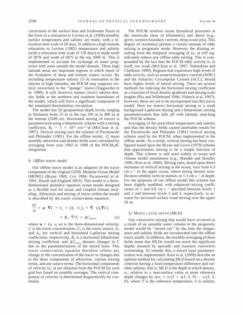
FIG. 1. Monthly Hovmoller plot of zonally averaged mixed layer depths: (a) observed (Kara et al. 2003), (b) CFC0.2, (c) CFC0.4, and (d)CFC0.8. Italicized numbers at the top of each plot represent the maximum zonally averaged MLD (m) each month.

and the pressure P 5 0. Kara et al. (2000) use a referencedepth of 10 m; in our model study we use the surfacemodel level (which is centered at 12.5 m); DT is aconstant temperature difference that is optimized by theauthors to give the best possible agreement between theWorld Ocean Atlas (Levitus et al. 1994) dataset and ahigh-resolution climatological time series from thenortheastern Pacific Ocean. The resulting optimal tem-perature difference that they find for this region is DT5 0.88C.

Preliminary results using POCM T and S showed thatthe DT 5 0.88C criteria results in maximum MLDs sig-nificantly greater than those estimated by Kara et al.(2003) for the global ocean (see Figs. 1a,d). As a result,two other criteria DT 5 0.28 and DT 5 0.48C wereimplemented (Figs. 1b,c). Best agreement for maximummonthly mixed layer depths was evident with the formercriteria and, as such, DT 5 0.28C was chosen for thelong integration idealized tracer experiments (see sec-tion 2c). The 12 monthly averaged ‘‘convection masks’’are calculated prior to the model integrations as a furthercomputational saving. The use of a seasonally varyingMLD parameterization represents an important im-

provement over previous offline studies (Ribbe andTomczak 1997; Stevens and Stevens 1999), which useannually averaged schemes and a result underestimatethe depth of convective mixing

2) UPTAKE OF CFCS

The air–sea fluxes for the CFC experiments were setup following experiment CF4 of England et al. (1994).Atmospheric CFC-11 concentrations where taken frommeasurements by Prinn et al. (2000) who give yearlyNorthern and Southern Hemisphere concentrations be-tween 1930 and 1999. Atmospheric concentrations wereinterpolated to monthly values in order to match the off-line model forcing and a smoothing function was appliedbetween 308N and 308S. CFC solubility, a, was calcu-lated using POCM temperature and salinity values in theempirically derived formula of Warner and Weiss (1985).The air–sea flux, QCFC, is proportional to the differencebetween the saturation concentration aCatm and the actualsurface water concentration Cw, namely,

Q 5 k(aC 2 C ).CFC atm w (2)


The value for the gas transfer speed k was taken fromthe empirical formulation of Wanninkhof (1992), whosuggests a dependence of k on the steady wind speed(U) squared. We also reduce QCFC in proportion to thesea ice cover R, which is assigned a value between 0and 1 depending on the mean ice coverage at a givenpoint. The exact formulation of k is then

21/2Sc2k 5 0.31U (1 2 R), (3)1 2660

where Sc is the temperature-dependent Schmidt number(Wanninkhof 1992). The wind dataset was taken fromthe mean monthly climatology of Esbenson and Kushnir(1981). The ice coverage data were taken from the recent18 climatology of Reynolds et al. (2001) and 12 monthlymeans were calculated from the 18 years of observa-tional data. Both ice and wind datasets were interpolatedonto the offline model grid using nearest-neighbor andlinear interpolation methods, respectively.

c. Tracer experiments

A series of four CFC-11 experiments, CFC0, CFC0.2,CFC0.4, and CFC0.8 were integrated with surface CFC-11 concentrations calculated by the method describedabove, with no parameterized mixed layer (CFC0) andmixed layers based on a DT 5 0.28, DT 5 0.48, andDT 5 0.88C criteria, respectively [see section 2b(2)].All experiments were integrated from 1935 to 1999 us-ing the atmospheric CFC-11 concentrations of Prinn etal. (2000)].

Experiments in which the tracer source is removedfrom the surface and is instead released from prescribedinterior regions no longer provide an absolute indicationof surface ventilation time scales [such an approach wasused by Hirst (1999)]. They do, however, provide auseful tool for examining interior ventilation pathwaysindependent of the representation of deep-water for-mation processes (such as open-ocean convection anddownslope flows). Stronger deep tracer signals alsomake pathways easier to identify. Two 1000-yr passive-tracer integrations were carried out in this regard. Thepassive tracer is only altered via the model’s advectionand mixing processes, with no decay term, therebytracking source water ventilation in the model interior.In the first (CNADW), 100% passive tracer is set in theNorth Atlantic Ocean north of 508N between 708W and308E at depths greater than 985 m. In the second (CBW),100% passive tracer is set in four Antarctic regions atdepths greater than 2750 m (the Weddell Sea south of658S between 658 and 108W; the Ross Sea between1608E and 1608W, and south of 708S; Amery Regionand south of 608S between 608 and 908E; and the AdelieRegion south of 608S between 1408 and 1508E). Bothexperiments, CNADW and CBW used MLD criteria equiv-alent to the CFC0.2 experiment. (Additional animated

sequences from the tracer experiments are available on-line at www.maths.unsw.edu.au/;alexg/.)

3. Results from CFC experiments

Dutay et al. (2002) compare the ability of 13 modelsparticipating in the Ocean Carbon Intercomparison Pro-ject (OCMIP) to reproduce observations of CFC-11 dis-tributions measured during WOCE. Various observedand model sections were compared using depth inte-grated CFC-11 inventories. A quantitative measure forcomparing the mean depth of penetration is also used.This is defined as the depth-integrated inventory dividedby the surface concentration at each horizontal position.These provide a useful standard set of tests by whichto compare the models.

a. North Atlantic

NADW originates primarily from two regions: 1) theLabrador Sea, which exports Labrador Sea Water (LSW)formed through open-ocean deep winter convection, and2) across the Greenland–Iceland–Scotland Ridge, whichexports Iceland–Scotland overflow water and DenmarkStrait overflow water into the North Atlantic. The exportof NADW southward is via a double-cored deep westernboundary current (DWBC) that follows the continentalshelf of eastern America. The upper core is made up ofthe less dense Labrador Sea waters, while the lower coreis sourced by the overflow waters.

Figure 2a shows CFC-11 values from the NationalOceanic and Atmospheric Administration’s EasternNorth Atlantic section (July–August 1993) nominallyalong 208W extending from 58S to Iceland (Castle et al.1998), hereinafter referred to as NA20W (as per Dutayet al. 2002). A fairly homogeneous CFC layer corre-sponds to mode water at ;388–458N centered at ;500-m depth. This is formed through deep convection andmakes up much of the water between the seasonal ther-mocline and the main thermocline at about 600 m (Do-ney and Bullister 1992). Between 158 and 208N a per-sistent front is evident at the southern edge of the sub-tropical gyre where low concentration South AtlanticCentral Water (SACW) advected from upwelling re-gions to the east abuts more recently ventilated NorthAtlantic Central Water (NACW) (Stramma and Siedler1988; Kawase and Sarmiento 1985). At greater depthsa high CFC signal of LSW can be seen extending southbeyond ;408N centered just below 1500 m. The onlyevidence of the denser overflow waters along theNA20W section is within the lower Iceland Basin (near558–608N). In the equatorial region a subsurface max-imum is evident between 1500 and 2000 m with a weak-er maximum visible between 3500 and 4000 m. Bothcores are displaced between 28 and 58 south of the equa-tor. Hydrographic and tracer studies have shown thatthese cores are a result of eastward advection of theDWBC within extra-equatorial jets (EEJs). These jets


FIG. 2. CFC-11 concentration (pmol kg21) for meridional NA20W section along 208W in the North Atlantic (Aug 1993): (a) observed,(b) CFC0, (c) CFC0.2, and (d) CFC0.4.

are persistent features of the equatorial region extendingto at least 108W for the upper jets that are not blockedby the Mid-Atlantic Ridge (Gouriou et al. 2001; Andrieet al. 1998). Eastward EEJs have been observed to occursymmetrically north and south of westward flowingequatorial deep jets (EDJs) that form a series of stackedeastward and westward flowing jets centered on theequator.

Many of the features observed along the NA20Wsection are captured by the CFC0.2 experiment (Fig. 2b).Mode water in the subtropical gyre has very similarmeridional and vertical extent, although the boundingmain thermocline is stronger due to a spurious CFCminimum below. This spurious feature is present in anumber of the OCMIP models (Dutay et al. 2002, theirFig. 5) and also in the eddy-permitting North Atlanticsimulation of Beismann and Redler (2003) who suggestthat it is due to poor ventilation of subtropical modewater. This is unlikely, though, as the minimum is belowthe depth of observed mode water penetration. More-over, in our model there is a distinct intrusion of lowCFC water into this region as part of the North AtlanticCurrent, which at intermediate depths (;1000 m) cor-responds to this minimum.

The front at the southern end of the subtropical gyreis more pronounced than observed and shifted almost58 farther north. Deeper in the water column there is astrong LSW signal penetrating to ;408N centered at;1700 m; however, the deeper overflow water observedin the Iceland Basin (558–608N) is entirely absent be-cause the model domain does not include the northernformation region where CFCs destined for the deeperNADW core would be absorbed. This is a clear weak-ness of the POCM in the context of global water-massventilation processes.

In the deep equatorial region the observed upper localtracer maximum is present between 18 and 28S centeredbetween 1750 and 2200 m, although it is significantlyweaker than observed. A further maximum is presentat the same position north of the equator (although atconcentrations below the lowest contour value) indi-cating the existence of an EEJ pair at this depth, withthe southern jet supplied with greater levels of tracer.Between 2750 and 3300 m centered directly on the equa-tor is a strong maximum. This represents the spuriousadvection of tracer advected in an EDJ from the DWBCat a depth that, in reality, would sit between the doubleDWBC core and so would be depleted in CFCs. The


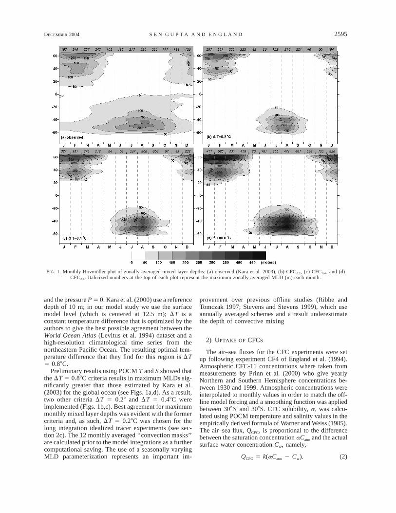
FIG. 3. CFC-11 column inventory (mol m22) along NA20W sectionfor observations and experiments CFC 0 , CFC 0.2 , CFC 0.4 , andCFC0.8.

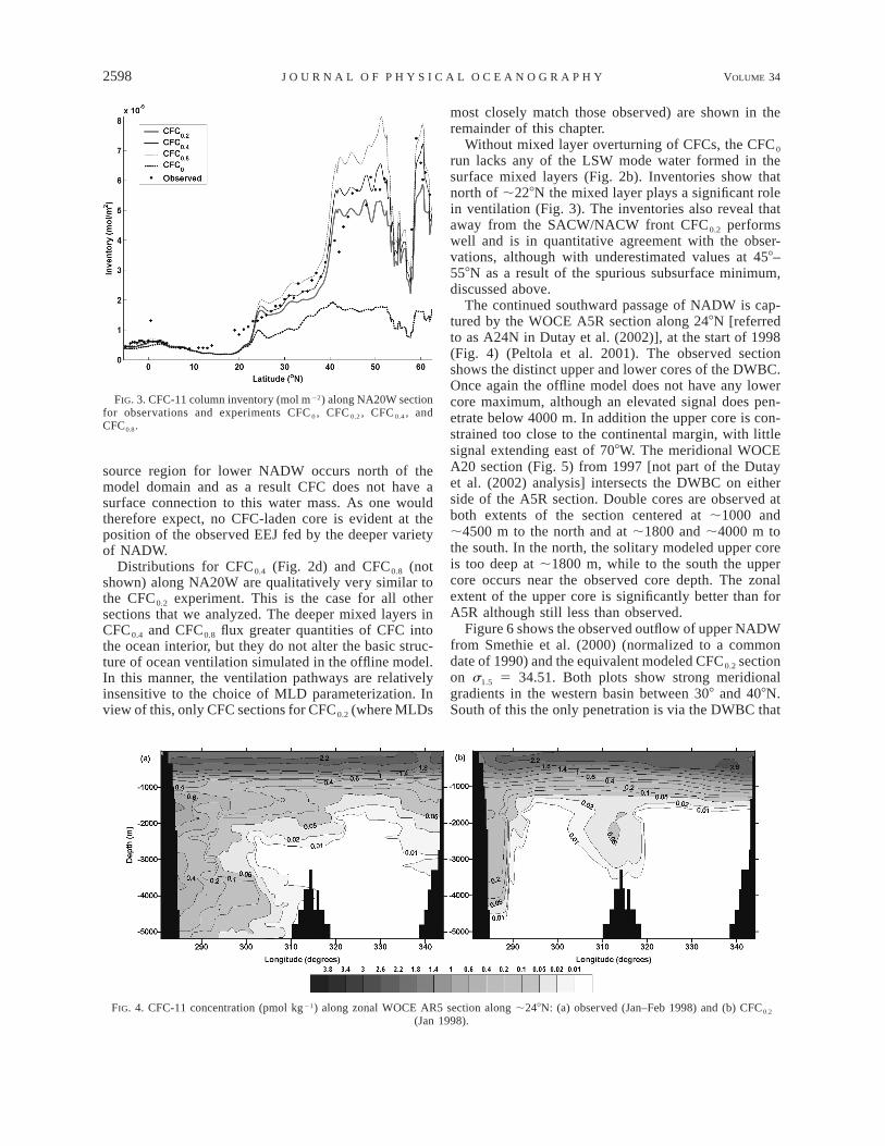
FIG. 4. CFC-11 concentration (pmol kg21) along zonal WOCE AR5 section along ;248N: (a) observed (Jan–Feb 1998) and (b) CFC0.2

(Jan 1998).

source region for lower NADW occurs north of themodel domain and as a result CFC does not have asurface connection to this water mass. As one wouldtherefore expect, no CFC-laden core is evident at theposition of the observed EEJ fed by the deeper varietyof NADW.

Distributions for CFC0.4 (Fig. 2d) and CFC0.8 (notshown) along NA20W are qualitatively very similar tothe CFC0.2 experiment. This is the case for all othersections that we analyzed. The deeper mixed layers inCFC0.4 and CFC0.8 flux greater quantities of CFC intothe ocean interior, but they do not alter the basic struc-ture of ocean ventilation simulated in the offline model.In this manner, the ventilation pathways are relativelyinsensitive to the choice of MLD parameterization. Inview of this, only CFC sections for CFC0.2 (where MLDs

most closely match those observed) are shown in theremainder of this chapter.

Without mixed layer overturning of CFCs, the CFC0

run lacks any of the LSW mode water formed in thesurface mixed layers (Fig. 2b). Inventories show thatnorth of ;228N the mixed layer plays a significant rolein ventilation (Fig. 3). The inventories also reveal thataway from the SACW/NACW front CFC0.2 performswell and is in quantitative agreement with the obser-vations, although with underestimated values at 458–558N as a result of the spurious subsurface minimum,discussed above.

The continued southward passage of NADW is cap-tured by the WOCE A5R section along 248N [referredto as A24N in Dutay et al. (2002)], at the start of 1998(Fig. 4) (Peltola et al. 2001). The observed sectionshows the distinct upper and lower cores of the DWBC.Once again the offline model does not have any lowercore maximum, although an elevated signal does pen-etrate below 4000 m. In addition the upper core is con-strained too close to the continental margin, with littlesignal extending east of 708W. The meridional WOCEA20 section (Fig. 5) from 1997 [not part of the Dutayet al. (2002) analysis] intersects the DWBC on eitherside of the A5R section. Double cores are observed atboth extents of the section centered at ;1000 and;4500 m to the north and at ;1800 and ;4000 m tothe south. In the north, the solitary modeled upper coreis too deep at ;1800 m, while to the south the uppercore occurs near the observed core depth. The zonalextent of the upper core is significantly better than forA5R although still less than observed.

Figure 6 shows the observed outflow of upper NADWfrom Smethie et al. (2000) (normalized to a commondate of 1990) and the equivalent modeled CFC0.2 sectionon s1.5 5 34.51. Both plots show strong meridionalgradients in the western basin between 308 and 408N.South of this the only penetration is via the DWBC that


FIG. 5. CFC-11 concentration (pmol kg21) along meridional WOCE A20 section (;528W): (a) observed (Jan–Feb 1998) and (b) CFC0.2

(Jan 1998).

FIG. 6. Lateral CFC-11 concentrations (pmol kg21) for ULSW: (a) observed distribution from Smethie et al. (2000) (data normalized to acommon date of 1990) and (b) CFC0.2 distribution on s1.5 5 34.51 kg m23 during Jun 1990.

branches at the equator, one part continuing as a DWBCinto the Southern Hemisphere and the other headingacross the Atlantic, constrained close to the equator. Asevidenced in the individual sections, the CFC0.2 DWBCsignal does not spread far enough to the east, with atight outflow locked to the western boundary. This islikely due to the lack of sufficient lateral eddy mixingin this region where eddy activity would be expectedto be high—a consequence of the temporal averagingof the advection fields or because the model fails tocapture small-scale recirculations that transport CFCseastward in observation.

b. Pacific OceanFigure 7a shows CFC-11 observations from the

WOCE P13 cruise nominally along 1658E in the North

Pacific during 1992. No significant CFC signal is ob-served below ;2000 m. Features observed along thissection are very similar to previous meridional sectionsin the western basin during 1987 and 1988 (Warner etal. 1996). Deepest penetration depths (.1100 m) occurwithin the subtropical gyre at ;308–358N. Penetrationdepths and inventories (Fig. 8) decrease southward witha front evident at the North Equatorial Current andCountercurrent divergence, at ;108N. The subtropicalgyre comprises primarily Subtropical Mode Water(STMW) formed by shallow winter convection, near thenortheastern limit of the gyre and advected laterally intothe gyre (Suga and Hanawa 1997), and within the lowerthermocline by North Pacific Intermediate Water(NPIW) formed through deep mixing in the Sea ofOkhostsk (Warner et al. 1996). Penetration depths in the


FIG. 7. CFC-11 concentration (pmol kg21) along meridional WOCE P13 section (;1658E): (a) observed (Aug–Oct 1992) and (b) CFC0.2

(Aug 1992).

FIG. 8. (a) CFC-11 column inventory (mol m22) and (b) penetration depths (m), along the WOCE P13 section for observations andexperiments CFC0, CFC0.2, CFC0.4, and CFC0.8.

subpolar gyre are much shallower (;400 m), a resultof the strong stratification and upwelling of low CFCconcentration deep waters.

CFC0.2 shows good qualitative agreement with ob-servations: shallow penetration in the subpolar region,increasing in the subtropical gyre with the intrusion ofsubsurface, high concentration mode water, and a weakfront once again across the north equatorial divergence.North of ;258N tracer inventories are generally un-derestimated. With no mixed layer deepening duringwinter the CFC0 run shows no mode water formation,only the recently ventilated waters being advected fromthe Sea of Okhostsk (;458N). The lack of STMW for-mation is a common feature to all the OCMIP models

(Dutay et al. 2002). The maximum penetration depth inour model CFC0.2 run is more than 200 m shallowerthan observation and occurs too far south.

c. Southern Ocean

Offline simulations are compared with two meridionalCFC sections: (i) the AJAX section (Fig. 9a) along theGreenwich meridian in 1983 (Warner and Weiss 1992)and (ii) the WOCE P15 section (Fig. 10a) along 1908Ein 1996. The observations reveal that the most extensivearea of newly ventilated water is the mode water, whichhas an almost circumpolar extent and is formed by openocean convection. This water travels northward in the


FIG. 9. CFC-11 concentration (pmol kg21) for AJAX section along Greenwich meridian: (a) observed (1983–84) and (b) CFC 0.2

(Dec 1983).

FIG. 10. CFC-11 concentration (pmol kg21) along WOCE P15 section (;1708W): (a) observed (Jan–Feb 1996) and (b) CFC0.2

(Feb 1996).

subtropical gyres as Antarctic Intermediate Water(AAIW). Other formation mechanisms for AAIW havebeen postulated including subduction along steep iso-pycnals and subsurface mixing; however, the relativeimportance of these processes is still in question (e.g.,Saenko et al. 2003; Santoso and England 2004). Southof the ACC poorly ventilated Circumpolar Deep Water(CDW), which may have undergone many circuitsaround Antarctica, rises near the Antarctic ‘‘Diver-gence.’’

Both sections show these generic Southern Ocean wa-termass features. Mode waters in the subtropical gyreshave their greatest penetration depths (not shown) be-tween 458 and 558S (P15) and between 408 and 508S(AJAX) reaching depths .1200 m and .750 m, re-spectively. Inventories gradually decrease northward(Fig. 11), although the AJAX section shows a smallincrease in the equatorial region where the surface wa-ters are subducted into the interior in a tropical over-

turning cell. Below the ventilated intermediate waterand extending southward CFC concentrations are lowbecause of the intrusion of CDW. Close to the Antarcticmargin at greater depths newly ventilated AABW bringselevated concentrations of CFC, although concentra-tions are substantially lower than surface values, as aresult of significant entrainment of poorly ventilated wa-ter during downslope flow. Once again, there is gen-erally a good qualitative agreement between simulationsand observations at surface and intermediate depths(Figs. 9 and 10). Column inventories are of a similarstructure (Fig. 11), although the observed northwardsspread of intermediate water is greater than in the model.

Upwelling of CFC-depleted CDW is well placed (near608S); however, both sections exhibit model column in-ventories substantially lower than observed (especiallyfor P15). The diminished eddy mixing of the offlinemodel in this area—normally associated with high eddyactivity—would reduce the lateral transport of tracer


FIG. 11. CFC-11 column inventory (mol m22) for observations and experiments CFC0, CFC0.2, CFC0.4, and CFC0.8 along (a) AJAXsection and (b) WOCE P15 section.

into these depleted regions, thus emphasizing the pro-nounced signal of low tracer concentration. This lowCFC inventory is unlike many coarse resolution oceanmodels that typically mix excessive amounts of CFCdownwards at these latitudes. This is evident in the col-umn inventories of the OCMIP models (Dutay et al.2002, their Fig. 11). England and Hirst (1997) also seethis in their coarse-resolution model experiments inwhich they use a variety of subsurface mixing param-eterizations. They find that the overestimated CFC con-centrations are directly related to deep convection that,in some experiments, penetrates almost to the oceanfloor. The offline model MLD parameterization, on theother hand, shows no deep convection south of 608S(Fig. 1). England and Hirst (1997) note improved resultsbelow 1000 m with the implementation of the Gent andMcWilliams mixing parameterization, which results inmore stratified conditions. Just north of the strongestupwelling, both simulated and observed AJAX sectionsshow the intrusion of recently ventilated water that hasbeen advected eastward along the northern limb of theWeddell gyre. Adjacent to the Antarctic margin, theoffline model reproduces some elevated concentrations;however, in both cases, inventories are smaller thanthose observed. No significant bottom water signal canbe seen extending northward at the abyssal depths alongboth AJAX and WOCE P15 sections. Formation of bot-tom water in OGCMs is often too weak in the SouthernOcean as a result of the poorly sampled and summer-biased observational data that are used to force the mod-el (e.g., Doney and Hecht 2002). In addition downslopeflow is particularly sensitive to the representation ofbottom topography, and the steplike nature of z-levelmodels has been shown to inhibit these flows (Beck-mann and Doscher 1997).

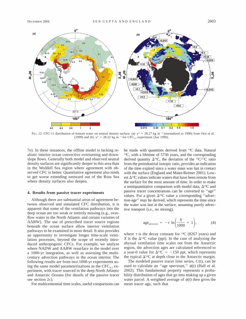
A recent analysis of WOCE sections in the SouthernOcean by Orsi et al. (1999) shows the distribution ofCFC within the AABW on the g n 5 28.27 kg m23

neutral density surface (Fig. 12). According to Orsi etal. (1999), this represents the lower bound neutral den-sity surface for Circumpolar Deep Water and, as such,surfaces exceeding this only contain water sourced onthe Antarctic shelf. These dense waters are completelyblocked at the Drake Passage and are thus decoupledfrom the overlaying eastward flowing Antarctic Circum-polar Current. Our simulated density values, calculatedfrom the POCM temperature and salinity fields, tend tobe slightly lower than observed. This is typical of z-level OGCMs (e.g., England and Hirst 1997). Conse-quently, for comparison with the observations wechoose a neutral layer (g n 5 28.22 kg m23) that moreclosely matches the lower limit for CDW surface. Wa-ters along this surface in the offline model are still atsufficient depth to be blocked at the Drake Passage, andno contamination by intermediate water is evident.

The best model agreement is in the Weddell Sea,where waters forming in the western region flow clock-wise along the northern perimeter of the Weddell gyreand then either northward near 308W as a westernboundary current into the Argentine Basin or back to-wards the south and west near 108–208E. A deep min-imum is evident in the central Weddell gyre region. Aregion of high tracer concentration (.1.6 pmol kg21)stretches from the western Weddell Sea to ;208E, ad-jacent to the margin. A similar pattern is seen in theRoss Sea; waters forming in the western part of the seaflow clockwise and then either recirculate at the easternedge of the Ross gyre or continue eastward while mov-ing closer to the continental margin. Concentrations are,however, generally lower than the observed by a factorof 2 or more. A strong signal is also evident near theAdelie coast (1408–1508E), but this fails to extend west-ward as observed, and the region of coastal waters be-tween 1508 and 508E are devoid of the high observedconcentrations that flow eastward from the Adelie coastand the Amery Ice Shelf (Orsi et al. 1999, their Fig.


FIG. 12. CFC-11 distribution of bottom water on neutral density surface: (a) g n 5 28.27 kg m23 (normalized to 1990) from Orsi et al.(1999) and (b) g n 5 28.22 kg m23 for CFC0.2 experiment (Jun 1990).

7e). In these instances, the offline model is lacking re-alistic interior ocean convective overturning and down-slope flows. Generally both model and observed neutraldensity surfaces are significantly deeper in this area thanin the Weddell Sea region where agreement with ob-served CFC is better. Quantitative agreement also tendsto get worse extending eastward out of the Ross Seawhere density surfaces also deepen.

4. Results from passive tracer experiments

Although there are substantial areas of agreement be-tween observed and simulated CFC distribution, it isapparent that some of the ventilation pathways into thedeep ocean are too weak or entirely missing (e.g., over-flow water in the North Atlantic and certain varieties ofAABW). The use of prescribed tracer source regionsbeneath the ocean surface allow interior ventilationpathways to be examined in more detail. It also providesan opportunity to investigate longer time-scale venti-lation processes, beyond the scope of recently intro-duced anthropogenic CFCs. For example, we analyzewhere NADW and AABW resurface in the model overa 1000-yr integration, as well as assessing the multi-century advection pathways in the ocean interior. Thefollowing results are from two 1000-yr experiments us-ing the same model parameterizations as the CFC0.2 ex-periment, with tracer sourced in the deep North Atlanticand Antarctic Oceans (for details of the passive tracersee section 2c).

For multicentennial time scales, useful comparisons can

be made with quantities derived from 14C data. Natural14C, with a lifetime of 5730 years, and the correspondingderived quantity D14C, the deviation of the 14C/12C ratiofrom the preindustrial isotopic ratio, provides an indicationof the time expired since a water mass was last in contactwith the surface (England and Maier-Reimer 2001). Low-est D14C values indicate waters that have been remote fromthe surface for the most amount of time. In order to makea semiquantitative comparison with model data, D14C andpassive tracer concentrations can be converted to ‘‘age’’values. For a given D14C value a corresponding ‘‘advec-tion-age’’ may be derived, which represents the time sincethe water was last at the surface, assuming purely advec-tive transport (i.e., no mixing),

Xage 5 2t ln 1 1 , (4)advection 1 21000

where t is the decay constant for 14C (8267 years) andX is the D14C value (ppt). In the case of analyzing theabyssal ventilation time scales out from the Antarcticregion, the advection ages are calculated referenced toa year-0 value for D14C 5 2150 ppt, which representsthe typical D14C at depth close to the Antarctic margin.

The modeled passive tracer time series, C(t), can beused to calculate an ‘‘age spectrum,’’ c(t) (Hall et al.2002). This fundamental property represents a proba-bility distribution of ages that go into making up a givenwater parcel. A weighted average of c(t) then gives themean tracer age, such that


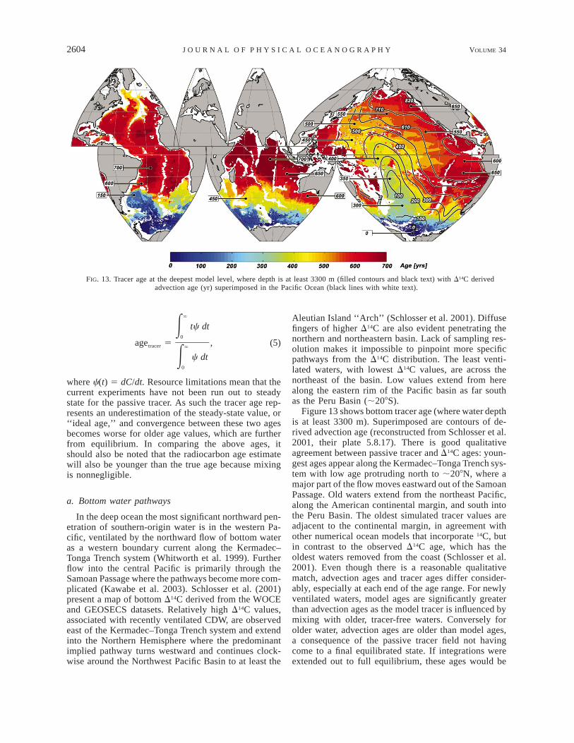
FIG. 13. Tracer age at the deepest model level, where depth is at least 3300 m (filled contours and black text) with D14C derivedadvection age (yr) superimposed in the Pacific Ocean (black lines with white text).

`

tc dtE0

age 5 , (5)tracer `

c dtE0

where c(t) 5 dC/dt. Resource limitations mean that thecurrent experiments have not been run out to steadystate for the passive tracer. As such the tracer age rep-resents an underestimation of the steady-state value, or‘‘ideal age,’’ and convergence between these two agesbecomes worse for older age values, which are furtherfrom equilibrium. In comparing the above ages, itshould also be noted that the radiocarbon age estimatewill also be younger than the true age because mixingis nonnegligible.

a. Bottom water pathways

In the deep ocean the most significant northward pen-etration of southern-origin water is in the western Pa-cific, ventilated by the northward flow of bottom wateras a western boundary current along the Kermadec–Tonga Trench system (Whitworth et al. 1999). Furtherflow into the central Pacific is primarily through theSamoan Passage where the pathways become more com-plicated (Kawabe et al. 2003). Schlosser et al. (2001)present a map of bottom D14C derived from the WOCEand GEOSECS datasets. Relatively high D14C values,associated with recently ventilated CDW, are observedeast of the Kermadec–Tonga Trench system and extendinto the Northern Hemisphere where the predominantimplied pathway turns westward and continues clock-wise around the Northwest Pacific Basin to at least the

Aleutian Island ‘‘Arch’’ (Schlosser et al. 2001). Diffusefingers of higher D14C are also evident penetrating thenorthern and northeastern basin. Lack of sampling res-olution makes it impossible to pinpoint more specificpathways from the D14C distribution. The least venti-lated waters, with lowest D14C values, are across thenortheast of the basin. Low values extend from herealong the eastern rim of the Pacific basin as far southas the Peru Basin (;208S).

Figure 13 shows bottom tracer age (where water depthis at least 3300 m). Superimposed are contours of de-rived advection age (reconstructed from Schlosser et al.2001, their plate 5.8.17). There is good qualitativeagreement between passive tracer and D14C ages: youn-gest ages appear along the Kermadec–Tonga Trench sys-tem with low age protruding north to ;208N, where amajor part of the flow moves eastward out of the SamoanPassage. Old waters extend from the northeast Pacific,along the American continental margin, and south intothe Peru Basin. The oldest simulated tracer values areadjacent to the continental margin, in agreement withother numerical ocean models that incorporate 14C, butin contrast to the observed D14C age, which has theoldest waters removed from the coast (Schlosser et al.2001). Even though there is a reasonable qualitativematch, advection ages and tracer ages differ consider-ably, especially at each end of the age range. For newlyventilated waters, model ages are significantly greaterthan advection ages as the model tracer is influenced bymixing with older, tracer-free waters. Conversely forolder water, advection ages are older than model ages,a consequence of the passive tracer field not havingcome to a final equilibrated state. If integrations wereextended out to full equilibrium, these ages would be


FIG. 14. Time evolution of the 1% passive tracer cencentration front, shown every 10 yr for the first 200 yr then at250, 300, and 400 yr (black contour lines show 50-, 100-, and 300-yr contours). Superimposed are the major impliedpathways. Legend: 1—Lousville Ridge; 2—Samoan Passage; 3—Manihiki Plateau; 4—Gilbert Ridge; 5—Wake IslandPassage; 6—Main Gap.

expected to increase somewhat. A global coarse-reso-lution tracer age simulation by England (1995), whichwas run out to equilibrium (taking 5000 years of inte-gration) showed maximum ages in the North Pacific atmiddepths of almost 1500 yr. This coarse model is inbroad qualitative agreement with our offline model andwith observations (England 1995, his Fig. 4d). However,the young-age signal extending along the Kermadec–Tonga Trench system extends only as far as the equator,a possible consequence of the sluggish boundary cur-rents evident in low-resolution models.

By looking at the time evolution of the model tracerfield it is possible to identify the major bottom-waterventilation pathways into the North Pacific. Figure 14shows the evolution of the 1% tracer concentration con-tour (at 10-yr intervals for the first 200 years and there-after at 220, 250, and 300 years) with the major impliedpathways superimposed. The simulated flow into thePacific basin occurs via two deep western boundary

currents along the Kermadec–Tonga and LouisvilleRidge systems that merge as the trenches come together,both flows are greatest at the deepest model levels. Thezonal WOCE P6 section across 328S of D14C (Schlosseret al. 2001) shows two areas of maximum D14C, the firstflanking the Kermadec–Tonga Ridge between 3500 and4500 m (well above the seafloor) and the second eastof the Louisville Ridge at the bottom. The majority ofnorthward flow travels through the Samoan Passage,with a smaller flow that passes anticlockwise around theManihiki Plateau, to the east of the passage, in broadagreement with observations (Roemmich et al. 1996).Some of this eastern flow fills the Penrhyn Basin to theeast, with the remainder continuing westward along thenorthern side of the plateau. The flow that has transitedthrough the Samoan Passage moves westward to theGilbert Ridge where it again bifurcates. The eastern flowbranches again at the northern edge of the Central Pa-cific Basin, with one part heading east toward the north-


east Pacific basin and the other entering the NorthwestPacific Basin through Wake Island Passage. The westernbranch continues northward, constrained to the west bythe ridge systems west of the Marian/Izu–Ogasawaratrenches and farther north by the continental margin.This is consistent with hydrographic measurements tak-en by Kawabe et al. (2003) and the general descriptiongiven by Mantyla and Reid (1983). Farther north, asynthesis of various studies of the Northwest PacificBasin is presented by Owens and Warren (2001). Thisprovides evidence of further pathways, in particular twoeastward branches off the western boundary current: onenorth of 258N that travels into the northeastern basinnorth of the Hawaiian Ridge; the other through the‘‘Main Gap’’ in the Emperor Sea Chain. The north-eastward flow of the western boundary current is alsoseen to continue towards the Aleutian Trench. These arealso the primary pathways followed by the simulatedtracer. Although some of the detailed flow pathways aredifferent between simulation and observation, overallagreement is good and much of the discrepancy is aresult of finescale differences in the bathymetry that playa major role in determining abyssal flow pathways.

Simulated northward flow into the Atlantic and Indianbasins is far less pronounced than in the Pacific withlittle tracer reaching into the Northern Hemisphere. Inthe Indian Ocean, northward penetration of simulatedbottom water occurs through a number of deep gaps inthe bounding ridge systems. A gap in the SouthwestIndian Ridge south of South Africa feeds the Aghulasand Mozambique Basins, with water derived from theWeddell Sea, where tracer is subsequently blocked fromcontinuing any farther northward by shallow topographyin the Mozambique Channel and by the MadagascarRidge to the east. AABW from the Weddell and Ameryregions also flows around the western side of the Ker-guelen Plateau and fills the Crozet Basin, with flowaround the east of the plateau hindered by shallowertopography. A weak signal can be seen emanating fromthe Crozet Basin through channels in the Southwest In-dian Ridge and into the Madagascar Basin from whereit continues northward as a western boundary currentalong Madagascar. These pathways correspond to ob-served Indian Ocean outflows of water leaving the Wed-dell Sea (Haine et al. 1998; Mantyla and Reid 1995).A further pathway is evident sourced from the eastwhere AABW fills the Australian–Antarctic Basin andcontinues northward through the Southeast Indian Ridgevia the Australian–Antarctic ‘‘Discordance.’’ This routebetween the basins is clearly seen in the property mapsof Mantyla and Reid (1995). Flow continues westwardand northward along the northern flank of the ridge intothe central Indian Ocean. Pathways into the NorthernHemisphere are more diffuse although some penetrationis evident on both sides of the central Indian Ridge withlittle signal in the eastern basin.

In the Atlantic, much of the simulated tracer sourcedfrom the Weddell Sea region is blocked from direct

northward transport by a system of ridges, primarily theSouth Scotia Ridge. Some northward movement is ev-ident through gaps into the Scotia Sea; however, themajority of the tracer destined to go north first travelseast around the South Sandwich Trench. Arhan et al.(1999) identifies three routes for Weddell Sea Water intothe Argentine Basin (the northern limit of the majorityof northward flowing water): (i) across the relativelyshallow Falkland Plateau (;2500 m), (ii) through a widebreach in the Falkland Ridge (;358–408W), and (iii) tothe east of the Islas Orcadas Ridge (;258W). The modelbathymetry however, dictates that the only significantsimulated deep pathway is via the third, eastern, option.The simulated filling of the Argentine Basin is via anetwork of pathways spanning the basin. In contrast,Orsi et al. (1999) describe only a single pathway ven-tilating the Argentine Basin, sourced primarily throughthe the breach in the Falkland Ridge. In the easternAtlantic, a weaker tracer signal, fed from water comingoff the northeastern rim of the Weddell gyre that hasexited the Southern Ocean through gaps in the South-west Indian Ridge, penetrates as far north as the NamibiaAbyssal Plain. The lack of vertical resolution at depthwill necessarily imply that many small-scale pathwayswill not be in agreement with observation. In addition,the model’s representation of bathymetry is somewhatcrude in certain locations (as also noted by Thorpe etal. 2004). Thorpe et al. note that bathymetry errors alsoresult from the interpolation methods used to generatethe POCM bathymetry. This model–observed mismatchin bathymetry drives some of the erroneous bottom wa-ter pathways noted above.

b. Recirculation of bottom water

At middepths .;2000 m, tracer concentrationsacross the basins are very low. In the Pacific region acomparison can be made along the zonal WOCE P6section. Figure 15 shows a comparison between D14Cadvection ages at 328S and the corresponding model-derived tracer age. Oldest ages are observed at mid-depths (;2000–3000 m) with two distinct maxima, at1558W in the central Southwest Pacific Basin and at758W along the Chilean continental margin, both cen-tered at ;2600 m. Schlosser et al. (2001) suggest thatthese correspond to two cores of the return flow of Pa-cific Deep Water, the ocean’s oldest water mass. Passivetracer results along the same section also show two areasof low tracer. The western area spreads from the Ker-madec–Tonga Ridge into the Southwest Pacific Basincentered at a similar depth to the observed D14C agemaximum. The eastern area again flanks the Chileanmargin, but takes its oldest values at the deepest levelsand extends too far to the west.

The fate of recirculated bottom water can be tracedto the surface by assessing final concentrations of CBW

in the upper model level (Fig. 16) and the zonal meanof passive tracer (Fig. 17a) at year 1000. The majority


FIG. 15. Tracer age (yr) across the P06 section at 328S. (a) Calculated from D14C values taking D14C 5 2150 ppt to be zero age (bottomwater close to the Antarctic margin has D14C ø 2150 ppt). (b) Calculated using the 1000-yr ‘‘age spectrum’’ derived from CBW concentrationsintegrated over 1000 yr.

of passive tracer upwells strongly close to the Antarcticmargin and along the northern edges of the Weddell andRoss gyres, where the divergence of surface waters aidsin pulling up deeper waters. Tracer levels remain highin these regions (south of the Antarctic divergence) andwithin the gyres where the tracer is quickly mixed. SomeCBW tracer gets mixed into the high energy ACC and isthen zonally distributed throughout the Southern Ocean.Even though there is no explicit representation of tracerrelease at the formation regions of AAIW, entry into theAtlantic, Pacific, and Indian Oceans is predominantlyas recycled intermediate water at depths between ;500and 1500 m (Fig. 17a). This is intensified in the easternbasin under the influence of the various anticyclonicsubtropical gyres. In the Pacific there is an additionalstrong surface penetration of tracer in the eastern basinwhere mixed layers are deep (see Fig. 15, where youngages generally correspond to high tracer concentrations).Lowest ages are at intermediate depths and near thesurface in the eastern Pacific. Farther north the elevatedtracer values within intermediate water becomes lessdistinct, practically disappearing north of the zone ofinfluence of the subtropical gyres, as basinwide up-welling moves the tracer into the surface layers.

c. North Atlantic Deep Water

Figure 18 shows passive tracer from CNADW at thedepth of maximum outflow (centered at 2475-m depth)after 100, 300, and 1000 years of integration. This depthis below the upper NADW core tagged by CFC dis-cussed in section 3a. From the source region two pre-dominant deep pathways are evident. A clear signal trav-els along the eastern boundary of the Mid-AtlanticRidge (MAR) centered at or above the top of the ridge.Large quantities of tracer leak westward across the topof the ridge and through the numerous fracture zones.

Below ;258N the signal dies away as the ridge becomesdeeper. Hydrographic sections investigating the spreadof LSW, taken over an 8-yr period in the region of theAzores Plateau (Paillet et al. 1998), show a persistentcurrent above the eastern flank of the MAR that extendsat least as far south as the Oceanographer Fracture Zone(;348N) where much of the flow feeds into the westernbasin.

The second pathway is the distinct DWBC along theAmerican continental margin. Zonal tracer sections (notshown) reveal that the core of this flow generally re-mains centered at a depth of ;2500 m, with elevatedconcentrations of tracer often evident between the po-sition of the observed double cores that represent upperand lower NADW. Many of the climate models inves-tigated by Dutay et al. (2002) show a similar single CFCmaximum at this intermediate depth. Like the passivetracer, the POCM meridional velocities (not shown)show no double core. This implies that the missing coreis not simply due to the lack of realistic tracer ventilationinto the interior at the tracer source region, but is likelyto be the result of poorly represented overflow processes(resulting in excessive entrainment of surrounding wa-ter) south of the Greenland–Iceland–Scotland ridges. Inan eddy-permitting model of the Atlantic, Beismann andRedler (2003) only obtain a lower core once a BBLscheme is incorporated into their model. In the case ofour CFC experiments a well-situated upper core is re-produced, demonstrating the ability of the model to formrealistic waters to feed the upper core. In contrast thenorthern limit of the POCM simulation (;658N) pre-cludes the lower CFC core originating in the Greenland–Iceland–Norwegian Sea. The DWBC can be traceddown as far as ;458S where it abruptly turns eastwardand is advected in a broad flow (initially between 408and 458S) as part of the ACC.


FIG. 16. Global tracer concentration of CBW (%) at the surface model level after 1000 yr of integration time.

FIG. 17. Zonal mean passive tracer (%) for (a) CBW global ocean, (b) CNADW North Atlantic, and (c) CNADW Pacific Ocean. Themeridional overturning streamfunction (Sverdrups) is superimposed (black contours) for the (a) global and (b) North Atlantic regions.

Between the source region and the point of its ultimateseparation from the American margin, the DWBCbranches a number of times primarily at the depth of thegreatest signal. At the equator a tightly constrained signalwith ;18 meridional extent, centred at ;½8N and witha maximum concentration between 2750 and 3300 m,propagates eastward across the basin in an equatorial jet,branching to the north and south on reaching the Africancoast. Numerous observations have been made of thesejets using hydrographic data to infer geostrophic currents(Zangenberg and Siedler 1998), from direct current mea-surements using lowered acoustic Doppler profilers(Gouriou et al. 2001, 1999), and from tracer measure-ments (Andrie et al. 1998). It has been shown that theyrepresent a permanent feature in each of the equatorialoceans. In fact, the structure is more complicated, com-prising a number of stacked jets with associated EEJsflowing in the opposite direction. No stacking can be

identified in the POCM simulation because the observeddistance between jets (;400–600 m) is comparable tothe vertical model resolution at this depth. Only a singlemaximum is evident, which is selectively sourced by theDWBC.

To the north of the equator a strong tracer signalbreaks away from the coast and recirculates to the north-west, bordered to the east by the MAR. A furtherbranching of this flow takes a majority of the tracerthrough a gap in the MAR at ;108N and northeastwardinto the central basin. Similar pathways were inferredbased on a transatlantic section along 118N (Friedrichsand Hall 1993) and on CFC observations (Smethie etal. 2000), which demonstrated the existence of a deeprecirculating gyre in the Guiana Basin running parallelto the continental shelf between the equator and ;208N.The simulated flow, however, lacks the observed north-ern return flow of the recirculating gyre, as the majority


FIG. 18. Concentration of CNADW (%) at the depth of greatest NADW outflow, model level 15 (2200–2750 m) (a) after 100 yr ofintegration, (b) at 300 yr of integration, and (c) at 1000 yr of integration.


FIG. 19. Global tracer concentration of CNADW (%) at the surface model level after 1000 yr of integration time.

of tracer is removed from the western basin through anunrealistically large gap in the MAR. Just south of theequator another offshoot heads southeastward, which atdepth is constrained within the Brazil Basin. This featureis in agreement with observations of Larque et al. (1997)who suggest two recirculations of NADW branching offthe DWBC; one just below the equator and the other at;108S.

The simulated DWBC branches once again in thevicinity of the Vitorio–Trinidade Ridge, which runs al-most perpendicular to the continental margin at ;208S.One branch heads southeastward away from the westernboundary; at depth this flow is constrained by the MARwhile shallower flow extends across the basin to theAfrican margin (from where it continues southward).Zangenberg and Siedler (1998) describe how potentialvorticity conservation and local topographic changeslead to this bifurcation.

After a long integration (see Fig. 18c) significant lev-els of tracer get mixed eastward across the Atlantic basinat mid- and deep levels. At depths shallower than theDWBC core, any upwelled tracer is strongly constrainednorth of the southern tip of South Africa. Here, entryof tracer-free Indian Ocean origin waters within theAghulas Current results in a sharp drop in tracer con-centrations. The intrusion of ‘‘return flow’’ waters tak-ing the so-called ‘‘warm route’’ from the Indian Ocean(Gordon 1986) in the upper branch of the thermohalinecirculation is thus important over a large proportion ofthe mid to upper water column. Stramma and Siedler(1988) present an analysis of WOCE data that showsinput of Indian Ocean waters to depths of at least 1200m. Below this, but most strongly between 2200 and 2750m, the DWBC continues southward along the westernboundary until it finally separates from the coast northof 458S and flows eastward as part of the ACC. During

its eastward transit the depth of maximum tracer shoalsfrom 2200 to 2700 m at the point of separation to be-tween 1300 and 2200 m within Drake Passage, after acomplete circuit of Antarctica. This is associated withthe large-scale upwelling of NADW and one of its byproducts, CDW. Idealized age tracer (Stevens and Ste-vens 1999) and Lagrangian particle (Doos 1995) ex-periments based on the flow field of the Fine-ResolutionAntarctic Model (FRAM) show a similar shoaling.

At the surface, significant levels of resurfacing CNADW

tracer are only evident south of the Aghulus Currentintrusion and extends as a continuous band stretchingaround the Southern Ocean (Fig. 19). This tracer hasbeen upwelled through deep convective mixing and Ek-man divergence in the Southern Ocean, fed by the deepsouthernmost branch of NADW. Some northward intru-sion of NADW into the southern portions of the Indianand Pacific Oceans occurs in the upper levels via thevarious surface currents (most notably the HumboldtCurrent). However, even after the 1000-yr integration,surface tracer levels are small. As with the CBW exper-iment there is a significant export of CNADW tracer intothe Indian and Pacific basins as intermediate water (Fig.17c). The most significant northward penetration, how-ever, occurs in the deep Pacific basin along pathwayscommon to the lower CDW (see section 4a).

5. Discussion and conclusions

We have developed an offline tracer transport modelrun at an eddy-permitting resolution to investigate in-terior ventilation pathways on interdecadal to intercen-tennial timescales. Ventilation on interdecadal timescales is assessed through a comparison between mod-eled CFC-11 tracer, incorporating a variety of MLDcriteria, and observations. Modeled intercentennial ven-


tilation is assessed through comparisons with observedD14C. The offline methodology has allowed us to inte-grate the ventilation experiments for unprecedentedlengths of time at eddy-permitting resolutions, provid-ing a cost-effective way to assess interior ventilation inhigh-resolution simulations.

The use of an eddy-permitting grid significantly im-proves the fidelity of an ocean model. The lower-res-olution OCMIP models (Dutay et al. 2002) showed sig-nificant intermodel variability in tracer inventory andpenetration depths, with the respective models perform-ing very differently along separate sections. Our offlinemodel performed consistently well over all analyzedsections, capturing most of the observed large-scale ven-tilation features, apart from the lower NADW core. Theimproved fidelity was, however, dependent on incor-poration of a seasonally varying MLD parameterizationthat captured open ocean convection during wintertimeevaporation and cooling of the surface layer. Withoutthe MLD parameterization, CFC-11 inventories fell farbelow observations in the areas where convective pro-cesses were important. The method of parameterization(Kara et al. 2000) gave a realistic spatial distribution ofMLDs (Fig. 1 shows zonally averaged information) withthe best agreement in areas of deep penetration. Therewas poorer representation of the widespread shallowmixed layers, evident particularly in the Southern Hemi-sphere oceans. This, however, was a consequence of thelack of shallow mixed layers in the original POCM-derived temperature field. Thorpe et al. (2004) note ex-cessively strong density gradients in the surface levelsof the POCMp4C simulations, which inhibit these wide-spread shallow mixed layers. They suggest that this isa result of use of the Pacanowski and Philander (1981)vertical mixing scheme, which was designed primarilyfor tropical regions and tends to underestimate surfacemixing at high latitudes. This problem was mitigated,to some extent, by our use of an increased vertical dif-fusion coefficient across the uppermost model levels tomimic the wind-driven mixing over the upper 50 m ofthe ocean. An MLD criterion of DT 5 0.28C gave themost realistic mixed layer depth distribution. This issmaller than the optimal criteria calculated by Kara etal. (2000) of DT 5 0.88C. A comparison between ob-served (Levitus et al. 1994) and POCM potential density(not shown) reveals that the modeled isopycnals areoften steeper than observed in regions where deep con-vection is prevalent. This explains why we obtained themost realistic MLD field with the smaller (DT 5 0.28C)criterion. An additional CFC integration performed us-ing the observed MLDs of Kara et al. (2003) producedresults very similar to the CFC0.2 experiment, except forsmall changes in the depth of penetration of some ofthe mode waters.

The simulation performs particularly well at captur-ing thermocline, mode, and surface waters. An analysisof surface CFC-11 concentrations along the various sec-tions (not shown), however, demonstrates that the pa-

rameterization of CFC uptake generally results in someunderestimation of modeled surface values at higherconcentrations. At greater depths agreement generallybecomes poorer. The upper core of NADW is presentas a fast-flowing boundary current; however, CFC-11concentrations are weaker than observed and do notspread far enough from the western boundary. The east-ward spread might be expected to be greater if the offlineeddy mixing had not been diminished by averaging.However, this does not seem to be the case, because theonline eddy-permitting model of Beismann and Redler(2003, their Fig. 5b) shows a CFC-laden boundary cur-rent that is equally constrained. Beismann and Redleralso compare their eddy-permitting model flow with thatof a coarse-resolution model and note that at sub-eddy-permitting resolutions the DWBC becomes overly dif-fuse and sluggish and a distinct western boundary pref-erence is only evident south of ;208N. This is in con-trast to the eddy-permitting models that form a tightlyconstrained, fast-flowing, boundary current that be-comes distinct at ;308N. Most of the coarse-resolutionOCMIP models show an indistinct DWBC with unre-alistic spreading of CFC eastward and insufficient south-ward penetration (Dutay et al. 2002).

The lower NADW core is entirely absent in our sim-ulations as a result of the model domain not encom-passing the formation zone of overflow waters, whereatmospheric CFC comes into contact with these densewaters. It is noted, in addition, that no distinct lowercore can be seen in the POCM velocity fields, despitethe northern ‘‘sponge’’ layer restoring model T–S toobservations north of 588N. Bottom-water CFC-11 con-centrations, although in good qualitative agreement inthe region of the Ross and Weddell gyres, are generallytoo weak and the extensive area of high CFC-11 ob-served between 808 and 1508E is entirely missing. Thesimulation of the formation and subsequent spread ofdeep and bottom waters in both the North Atlantic andaround Antarctica represents a difficult challenge be-cause many processes are involved: air–sea–ice inter-action during formation, deep convection or overflowwith consequent entrainment of other waters, BBLflows, and deep circulation patterns. The weak forma-tion of AABW is a common problem of many OGCMsthat are forced by temperature and salinity climatologies(e.g., Ribbe and Tomczak 1997); these climatologies aregenerally biased toward summer conditions, when for-mation is weak or absent. As such, it is not surprisingto find that most studies poorly represent these deepflows. Some improvement has been demonstrated whena bottom boundary layer scheme is implemented (Cam-pin and Gosse 1999; Doscher and Beckmann 2000; Nak-ano and Suginohara 2002) in z-coordinate models. TheBBL schemes result in stronger outflow currents andless entrainment. For instance, the incorporation of aBBL scheme in the eddy-permitting model of Beismannand Redler (2003) sufficiently improved overflow pro-cesses in order to produce the previously absent lower


core of NADW. Unfortunately, the altered flow char-acteristics associated with a BBL scheme make it dif-ficult to incorporate into an offline model where theadvective fields are not prognostic. It would also distortthe assessment of the online model ventilation as newphysics would have to be introduced into the offlinemodel.

For the multicentury integrations the inadequacies inrepresenting deep ventilation can be removed by spec-ifying interior source regions for the passive tracer. Thecomparison of tracer ages within the Pacific showedgood qualitative agreement with observed D14C age es-timates: significant penetration of young bottom waternorthward along the Kermadec–Tonga Trench systemfollowed by a clockwise spreading into the northernbasin, oldest bottom water situated along the northeastbasin (Fig. 13), and old water centered in two coresreturning southward at middepth (Fig. 15). In many re-gions, however, the age values were not in agreement.This is not necessarily a failing of the simulation; it maybe a consequence of the different effect that mixing hason tracers with different source functions and decayproperties (Waugh et al. 2003). The model age field isalso not necessarily at steady state. In short, direct com-parison between the absolute model age and D14C de-rived advection age is ambiguous; it is more appropriateto simply compare pathways of penetration of youngwaters in the model and observed estimates.

The coarse resolution of D14C measurements preventsidentification of detailed ventilation pathways. How-ever, existing hydrographic surveys do provide a broadpicture of deep and bottom water ventilation routes.When we study the idealized tracer of deep North At-lantic source water, the simulated southward passage ofNADW as a DWBC is primarily as a single diffuse core.The maximum outflow layer is located between the ob-served double core. The lack of a double core stems inpart from our use of an extended source region in thevertical, implying that the boundary current may be fedby a variety of densities, and from poorly representedoverflow processes, which entrain excessive surround-ing water during the overflow of the deeper core. Thisis in contrast to the real ocean that sees only two distinctdensities (i.e., LSW and Denmark Strait overflow water)spiked with young waters. Apart from this shortcoming,many of the observed bifurcations in the flow are rep-resented, including some of the structure evident in theequatorial region. The pathways that branch off the mainflow often extend too far across the Atlantic basin,where in reality these branches tend to recirculate andre-merge with the boundary current. The simulation cor-rectly represents the final separation of the DWBC tojoin the ACC. In the Southern Ocean, predominantlywithin the ACC region, mixing with waters from belowincreases NADW tracer concentrations at depth fromwhere northward penetration occurs in the lower modellevels. Alternatively mixing with waters from above andthe circumpolar Ekman divergence brings elevated con-

centrations to intermediate and surface levels wherenorthward penetration occurs under the influence of thesurface currents.

Detailed bottom-water pathways are generally con-sistent with observations, with the main deep northwardventilation occurring in the Pacific, primarily as a seriesof western boundary currents constrained by the ba-thymetry and with a number of bifurcations to the east.The eastward bifurcations occur through various gapsin the central Pacific basin ridge systems. It should benoted, though, that only a small proportion of the bot-tom-water tracer actually flows northwards in the abys-sal ocean. Instead, it is largely upwelled south of theACC (Fig. 17a), where some of the tracer then flowsnorthward as part of AAIW. In contrast, most NADWflows out into the Southern Ocean, with only a smallfraction fluxed back to the surface (mainly via the mixedlayers exchanging deep and surface waters over winter,Fig. 17b). This difference between NADW and AABWis largely due to the ‘‘Drake Passage effect’’ (Toggweilerand Samuels 1995), which dictates that meridional geo-strophic flow across the Drake Passage gap is negligible(because zonal pressure gradients cannot develop with-out land masses). This means AABW sinking off Ant-arctica can only be replaced by upwelled CDW/NADW/AABW at the Drake Passage gap—not by upper watersto the north of the gap. In contrast, NADW is drawnout of the North Atlantic into the Southern Ocean sincethere is no substantial surface divergence (and deep up-welling) north of 308S (apart from that in the equatorialoceans, but this is thought to be weak in NADW content,and dominated moreover by the shallow equatorial over-turning cells (Toggweiler and Samuels 1995).

The offline methodology, when implemented withsuitable parameterizations to take account of the tem-poral averaging of the input fields, provides a powerfultool for the investigation of ventilation at high resolutionand over long time scales. The primary limitation is thelack of any possible feedback onto the model dynamics,thus making, for example, offline simulations of climatechange impossible. The offline model can, however, bean ideal tool for understanding the present-day oceanventilation. It also provides the only practical means forassessing interior ocean circulation regimes, at multi-century time scales, in models with eddy-permitting res-olution.

Acknowledgments. We thank Robin Tokmakian forproviding the POCM input data used in this study andthe APAC Australian national computing facility forcomputing resources and technical support. We alsothank our anonymous reviewers for their helpful com-ments. This project was supported by the AustralianResearch Council.

REFERENCES

Andrie, C., J. F. Ternon, M. J. Messias, L. Memery, and B. Bourles,1998: Chlorofluoromethane distributions in the deep equatorial


Atlantic during January–March 1993. Deep-Sea Res., 45A, 903–930.

Arhan, M., K. J. Heywood, and B. A. King, 1999: The deep watersfrom the Southern Ocean at the entry to the Argentine Basin.Deep-Sea Res., 46B, 475–499.

Aumont, O., J. C. Orr, D. Jamous, P. Monfray, O. Marti, and G.Madec, 1998: A degradation approach to accelerate simulationsto steady-state in a 3-D tracer transport model of the globalocean. Climate Dyn., 14 (2), 101–116.

Beckmann, A., and R. Doscher, 1997: A method for improved rep-resentation of dense water spreading over topography in geo-potential-coordinate models. J. Phys. Oceanogr., 27, 581–591.

Beismann, J. O., and R. Redler, 2003: Model simulations of CFCuptake in North Atlantic Deep Water: Effects of parameter-izations and grid resolution. J. Geophys. Res., 108, 3159,doi:10.1029/2001JC001253.

Bryan, K., 1969: A numerical method for the study of the circulationof the World Ocean. J. Comput. Phys., 4, 347–376.

——, and L. J. Lewis, 1979: A water mass model of the World Ocean.J. Geophys. Res., 84, 2503–2517.

Campin, J. M., and H. Goosse, 1999: A parameterization of denseoverflow in large-scale ocean models in z-coordinate. Tellus,51A, 412–430.

Castle, R. D., and Coauthors, 1998: Chemical and hydrographic pro-files and underway measurements from the eastern North At-lantic during July and August of 1993. NOAA Data Rep. ERLAOML-32 (PB98-131865), 82 pp.

Cox, M. D., 1984: A primitive equation, three-dimensional model ofthe ocean. GFDL Ocean Group Tech. Rep. 1, 250 pp.

Doney, S. C., and J. L. Bullister, 1992: A chlorofluorocarbon sectionin the eastern North Atlantic. Deep-Sea Res., 39A, 1857–1883.

——, and M. Hecht, 2002: Antarctic Bottom Water formation anddeep-water chlorofluorocarbon distributions in a global oceanclimate model. J. Phys. Oceanogr., 32, 1642–1666.

Doos, K., 1995: Interocean exchange of water masses. J. Geophys.Res., 100 (C7), 13 499–13 514.

Doscher, R., and A. Beckmann, 2000: Effects of a bottom boundarylayer parameterization in a coarse-resolution model of the NorthAtlantic Ocean. J. Atmos. Oceanic Technol., 17, 698–707.

Dutay, J. C., and Coauthors, 2002: Evaluation of ocean model ven-tilation with CFC-11: Comparison of 13 global ocean models.Ocean Modell., 4, 89–120.

England, M. H., 1995: Using chlorofluorocarbons to assess oceanclimate models. Geophys. Res. Lett., 22, 3051–3054.

——, and H. C. Hirst, 1997: Chlorofluorocarbon uptake in a WorldOcean model. Part 2: Sensitivity to surface thermohaline forcingand subsurface mixing parameterisation. J. Geophys. Res., 102,15 709–15 731.

——, and S. Rahmstorf, 1999: Sensitivity of ventilation rates andradiocarbon uptake to subsurface mixing parameterization inocean models. J. Phys. Oceanogr., 29, 2802–2827.

——, and E. Maier-Reimer, 2001: Using chemical tracers to assessocean models. Rev. Geophys., 39, 29–70.

——, V. C. Garcon, and J. F. Minster, 1994: Chlorofluorocarbon up-take in a World Ocean model. Part 1: Sensitivity to the surfacegas forcing. J. Geophys. Res., 99, 25 215–25 233.

Esbenson, S. K., and Y. Kushnir, 1981: The heat budget of the globalocean: An estimate from surface marine observations. ClimateResearch Institute, Oregon State University, Tech. Rep. 29, 27pp.

Friedrichs, M. A. M., and M. H. Hall, 1993: Deep circulation in thetropical North Atlantic. J. Mar. Res., 51, 697–922.

Gordon, A. L., 1986: Interocean exchange of thermocline water. J.Geophys. Res., 91, 5037–5046.

Gouriou, T., B. Bourles, H. Mercier, and R. Chuchla, 1999: Deep jetsin the equatorial Atlantic Ocean. J. Geophys. Res., 104 (C9),21 217–21 226.

——, and Coauthors, 2001: Deep circulation in the equatorial AtlanticOcean. Geophys. Res. Lett., 28, 819–822.

Haine, T. W. N., A. J. Watson, M. I. Liddicoat, and R. R. Dickson, 1998:

The flow of Antarctic bottom water to the southwest Indian Oceanestimated using CFCs. J. Geophys. Res., 103 (C12), 27 637–27 653.

Hall, T. M., T. W. N. Haine, and D. W. Waugh, 2002: Inferring theconcentration of anthropogenic carbon in the ocean from tracers.Global Biogeochem. Cycles, 16, 1131, doi:10.1029/2001GB001835.

Hazell, D., and M. H. England, 2003: Prediction of the fate of ra-dioactive material in the South Pacific Ocean using a globaleddyresolving model. J. Environ. Radio., 65, 329–355.

Hirst, A. C., 1999: Determination of water component age in oceanmodels: Application to the fate of North Atlantic Deep Water.Ocean Modell., 1, 81–94.

——, S. P. O’Farrell, and H. B. Gordon, 2000: Comparison of acoupled ocean–atmosphere model with and without oceaniceddy-induced advection. Part I: Ocean spinup and control in-tegrations. J. Climate, 13, 139–163.

Kara, B. A., P. A. Rochford, and E. Hurlburt, 2000: An optimaldefinition for ocean mixed layer depth. J. Geophys. Res., 105(C7), 16 803–16 821.

——, ——, and ——, 2003: Mixed layer depth variability over the globalocean. J. Geophys. Res., 108, 3079, doi:10.1029/2000JC000736.

Kawabe, M., S. Fujio, and D. Yanagimoto, 2003: Deep-water cir-culation at low latitudes in the western North Pacific. Deep-SeaRes., 50A, 631–656.

Kawase, M., and J. L. Sarmiento, 1985: Nutrients in the Atlanticthermocline. J. Geophys. Res., 90 (C5), 8961–8979.

Larque, L., K. Maamaatuaiahutapu, and V. Garcon, 1997: On theintermediate and deep water flows in the South Atlantic Ocean.J. Geophys. Res., 102 (C6), 12 425–12 440.

Levitus, S., 1982: Climatalogical Atlas of the World Ocean. NOAAProf. Paper 13, 173 pp. and 17 microfiche.

——, R. Burgett, and T. P. Boyer, 1994: Salinity. Vol. 3, World OceanAtlas 1994, NOAA Atlas NESDIS 3, 99 pp.

Manabe, S., and R. J. Stouffer, 1996: Low-frequency variability ofsurface air temperature in a 1000-year integration of a coupledocean–atmosphere–land surface model. J. Climate, 9, 376–393.

Mantyla, A. W., and J. L. Reid, 1983: Abyssal characteristics of theWorld Ocean waters. Deep-Sea Res., 30A, 805–833.

——, and ——, 1995: On the origins of deep and bottom waters inthe Indian Ocean. J. Geophys. Res., 100 (C2), 2417–2439.

McClean, J. L., A. J. Semtner, and V. Zlotnicki, 1997: Comparisonsof mesoscale variability in the Semtner–Chervin quarter-degreemodel, the Los Alamos sixth-degree model, and TOPEX/PO-SEIDON Data. J. Geophys. Res., 102 (C11), 25 203–25 226.

Nakano, H., and N. Suginohara, 2002: Effects of bottom boundarylayer parameterization on reproducing deep and bottom watersin a World Ocean model. J. Phys. Oceanogr., 32, 1209–1227.

Orsi, A. H., G. C. Johnson, and J. L. Bullister, 1999: Circulation,mixing, and production of Antarctic Bottom Water. Progress inOceanography, Vol. 43, Pergamon, 55–109.

Owens, W. B., and B. A. Warren, 2001: Deep circulation in the north-west corner of the Pacific Ocean. Deep-Sea Res., 40A, 959–993.

Pacanowski, R. C., and S. G. H. Philander, 1981: Parameterizationof vertical mixing in numerical models of tropical oceans. J.Phys. Oceanogr., 11, 1443–1451.

——, K. W. Dixon, and A. Rosati, 1991: The Geophysical FluidDynamics Laboratory Modular 755 Ocean Model users guide.Geophysical Fluid Dynamics Laboratory Ocean Group Tech.Rep. 2, 46 pp.

Paillet, J., M. Arhan, and M. S. McCartney, 1998: Spreading of Lab-rador Sea Water in the eastern North Atlantic. J. Geophys. Res.,103 (C5), 10 223–10 239.

Peltola, E., and Coauthors, 2001: Chemical and hydrographic mea-surements on a Climate and Global Change Cruise along 248Nin the Atlantic Ocean WOCE section A5R (repeat) during Jan-uary–February 1998. NOAA Data Rep. OAR AOML-41, 199pp.

Prinn, R. G., and Coauthors, 2000: A history of chemically and ra-diatively important gases in air deduced from ALE/GAGE/AGA-GE. J. Geophys. Res., 105, 17 751–17 792.

Reynolds, R. W., T. M. Smith, D. C. Stokes, and W. Wang, 2001: An


improved in situ satellite SST analysis for climate. J. Climate,15, 1609–1624.

Ribbe, J., and M. Tomczak, 1997: On convection and the formationof Subantarctic Mode Water in the Fine Resolution AntarcticModel—FRAM. J. Mar. Syst., 13, 137–154.

Rix, N. H., and J. Willebrand, 1996: Parameterization of mesoscaleeddies as inferred from a high-resolution circulation model. J.Phys. Oceanogr., 26, 2281–2285.

Roemmich, D., S. Hautala, and D. Rudnick, 1996: Northward abyssaltransport through the Samoan Passage and adjacent areas. J.Geophys. Res., 101 (C6), 14 039–14 055.

Saenko, O. A., A. J. Weaver, and M. H. England, 2003: A region ofenhanced northward Antarctic Intermediate Water transport in acoupled climate model. J. Phys. Oceanogr., 33, 1528–1535.

Santoso, A., and M. H. England, 2004: Antarctic Intermediate WaterCirculation and variability in a coupled climate model. J. Phys.Oceanogr., 34, 2160–2179.

Schlosser, P., J. L. Bullister, R. Fine, W. J. Jenkins, R. Key, J. Lupton,W. Roether, and W. M. Smethie Jr., 2001: Transformation andage of water masses. Ocean Circulation and Climate: Observingand Modelling the Global Ocean, S. Seidler et al., Eds., Inter-national Geophysical Series, Vol. 77, Academic Press, 431–452.

Semtner, A., and R. Chervin, 1992: Ocean general circulation froma globally eddy-resolving model. J. Geophys. Res., 97, 5493–5500.

Smethie, W. M., R. A. Fine, A. Putzka, and E. P. Jones, 2000: Tracingthe flow of North Atlantic Deep Water using chlorofluorocar-bons. J. Geophys. Res., 105 (C5), 14 297–14 323.

Stammer, D., R. Tokmakian, A. Semtner, and C. Wunsch, 1996: Howwell does a quarter-degree global circulation model simulatelarge-scale observations? J. Geophys. Res., 101, 25 779–25 811.

Stevens, I. G., and D. P. Stevens, 1999: Passive tracers in a generalcirculation model of the Southern Ocean. Ann. Geophys., 17,971–982.

Stramma, L., and G. Siedler, 1988: Seasonal changes in the NorthAtlantic sub-tropical gyre. J. Geophys. Res., 93, 8111–8118.

Suga, T. Y., and K. Hanawa, 1997: Thermostad distribution in the

North Pacific subtropical gyre: The subtropical mode water andthe central mode water. J. Phys. Oceanogr., 27, 140–152.

Thorpe, S., D. Stevens, and K. Heywood, 2004: Comparison of twotime-variant forced eddy-permitting global ocean models withhydrography of the Scotia Sea. Ocean Modell., in press.

Toggweiler, J. R., and B. Samuels, 1995: Effect of Drake Passage onthe global thermohaline circulation. Deep-Sea Res., 42A, 477–500.

——, K. Dixon, and K. Bryan, 1989: Simulations of radiocarbon ina coarse-resolution World Ocean model. Part 1: Steady stateprebomb distributions. J. Geophys. Res., 94 (C6), 8217–8242.

Tokmakian, R., and P. G. Challenor, 1999: On the joint estimation ofmodel and satellite sea surface height anomaly errors. OceanModell., 1, 39–52 and Erratum 119–125.

Visbeck, M., J. Marshall, T. Haine, and M. Spall, 1997: Specificationof eddy transfer coefficients in coarse resolution ocean circu-lation models. J. Phys. Oceanogr., 27, 381–402.

Wanninkhof, R., 1992: Relationship between wind speed and gasexchange over the ocean. J. Geophys. Res., 97 (C5), 7373–7382.

Warner, M. J., and R. F. Weiss, 1985: Solubilities of chlorofluoro-carbons 11 and 12 in water and seawater. Deep-Sea Res., 32A,1485–1497.

——, and ——, 1992: Chlorofluoromethanes in South Atlantic Ant-arctic Intermediate Water. Deep-Sea Res., 39A, 2053–2075.

——, J. L. Bullister, D. P. Wisegarver, R. H. Gammon, and R. F.Weiss, 1996: Basin-wide distributions of chlorofluorocarbons F-11 and F-12 in the North Pacific: 1985–1989. J. Geophys. Res.,101 (C9), 20 525–20 542.

Waugh, D. W., T. M. Hall, and T. W. N. Haine, 2003: Relation-ships among tracer ages. J. Geophys. Res., 108, 3138,doi:10.1029/2002JC001325.

Whitworth, T., B. A. Warren, W. D. Nowlin Jr., S. B. Rutz, R. D.Pillsbury, and M. I. Moore, 1999: On the deep western-boundarycurrent in the Southwest Pacific Basin. Progress in Oceanog-raphy, Vol. 43, Pergamon, 1–54.

Zangenberg, N., and G. Siedler, 1998: Path of the North AtlanticDeep Water in the Brazil Basin. J. Geophys. Res., 103 (C3),5419–5428.

evaluation of interior circulation in a high-resolution...

Documents