Naval Research LaboratoryStennis Space Center, MS 39529-5004

NRL/MR/7320--06-8984

Approved for public release; distribution is unlimited.

Evaluation of Delft3D Performancein Nearshore FlowsY. LarrY Hsu James D. DYkes ricHarD a. aLLarD

Ocean Dynamics and Prediction BranchOceanography Division

December 28, 2006

James m. kaiHatu

Texas A&M UniversityCollege Station, Texas

i

REPORT DOCUMENTATION PAGE Form ApprovedOMB No. 0704-0188

3. DATES COVERED (From - To)

Standard Form 298 (Rev. 8-98)Prescribed by ANSI Std. Z39.18

Public reporting burden for this collection of information is estimated to average 1 hour per response, including the time for reviewing instructions, searching existing data sources, gathering and maintaining the data needed, and completing and reviewing this collection of information. Send comments regarding this burden estimate or any other aspect of this collection of information, including suggestions for reducing this burden to Department of Defense, Washington Headquarters Services, Directorate for Information Operations and Reports (0704-0188), 1215 Jefferson Davis Highway, Suite 1204, Arlington, VA 22202-4302. Respondents should be aware that notwithstanding any other provision of law, no person shall be subject to any penalty for failing to comply with a collection of information if it does not display a currently valid OMB control number. PLEASE DO NOT RETURN YOUR FORM TO THE ABOVE ADDRESS.

5a. CONTRACT NUMBER

5b. GRANT NUMBER

5c. PROGRAM ELEMENT NUMBER

5d. PROJECT NUMBER

5e. TASK NUMBER

5f. WORK UNIT NUMBER

2. REPORT TYPE1. REPORT DATE (DD-MM-YYYY)

4. TITLE AND SUBTITLE

6. AUTHOR(S)

8. PERFORMING ORGANIZATION REPORT NUMBER

7. PERFORMING ORGANIZATION NAME(S) AND ADDRESS(ES)

10. SPONSOR / MONITOR’S ACRONYM(S)9. SPONSORING / MONITORING AGENCY NAME(S) AND ADDRESS(ES)

11. SPONSOR / MONITOR’S REPORT NUMBER(S)

12. DISTRIBUTION / AVAILABILITY STATEMENT

13. SUPPLEMENTARY NOTES

14. ABSTRACT

15. SUBJECT TERMS

16. SECURITY CLASSIFICATION OF:

a. REPORT

19a. NAME OF RESPONSIBLE PERSON

19b. TELEPHONE NUMBER (include areacode)

b. ABSTRACT c. THIS PAGE

18. NUMBEROF PAGES

17. LIMITATIONOF ABSTRACT

Evaluation of Delft3D Performance in Nearshore Flows

Y. Larry Hsu, James D. Dykes, Richard A. Allard, and James M. Kaihatu*

Naval Research LaboratoryOceanography DivisionStennis Space Center, MS 39529-5004 NRL/MR/7320--06-8984

Approved for public release; distribution is unlimited.

Unclassified Unclassified UnclassifiedUL 27

Y. Larry Hsu

(228) 688-5260

Delft3DWave height

The Delft3D modeling system, developed by Delft Hydraulics (www.wldelft.nl), is capable of simulating hydrodynamic processes due to waves, tides, rivers, winds, and coastal currents. It can be used to provide surf prediction for areas with complicated bathymetry where the use of a one-dimensional surf model is inappropriate. Delft3D has many model options and free parameters. The main objective of this investigation is to examine the effects of these selections on the performance of Delft3D. Both Duck94 and NSTS Santa Barbara data were used for evaluating Delft3D performance. Many parameters and options including roller, breaker delay, and breaking dissipation formulations are evaluated. All three bottom friction formulations, i.e., Chezy, White-Colebrook, and Manning, are evaluated and all can produce good longshore current results, if proper empirical bottom friction coefficient is used. The RMS error for longshore current is about 0.2 m/s.

28-12-2006 Memorandum Report

Space and Naval Warfare Systems Command2451 Crystal DriveArlington, VA 22245-5200

PE0602435N

ONR and SPAWAR

Longshore currentSurf

73-6729-07-5

*Texas A&M University, College Station, TX 77843

Office of Naval ResearchOne Liberty Center875 North Randolph StreetArlington, VA 22203-1995

CONTENTS

1. INTRODUCTION................................................................................................................................. 1

2. MODELDESCRIPTIONS.................................................................................................................... 1

3. FIELDDATAANDMODELSETUP................................................................................................... 2

3.1 Duck94Cases................................................................................................................................ 2 3.2 SantaBarbaraCases...................................................................................................................... 4

4. MODELRESULTS............................................................................................................................... 4

4.1 Duck94Cases................................................................................................................................ 4 4.1.1 Rollervs.NoRoller........................................................................................................... 4 4.1.2 BreakingDissipationFormulation..................................................................................... 6 4.1.3 BreakerDelay..................................................................................................................... 8 4.1.4 TurnOfftheRollerStressatVeryShallowWater.............................................................10 4.1.5 TheEffectofBottomFrictionSelection............................................................................12 4.2 SantaBarbara.................................................................................................................................20 4.2.1 Rollervs.NoRoller...........................................................................................................20 4.2.2 BreakingDissipationFormulation.....................................................................................21 4.2.3 BreakerDelay.....................................................................................................................21 4.2.4 TheEffectofBottomFrictionSelection............................................................................22

5. SUMMARYANDCONCLUSIONS....................................................................................................22

ACKNOWLEDGEMENTS........................................................................................................................23

REFERENCES...........................................................................................................................................23

iii

1

1. INTRODUCTION

The one-dimensional Navy Standard Surf Model (NSSM) has been shown to be very robust, but it has its limitations. Since NSSM assumes parallel bottom contours in the surf zone (generally depths of 8 m or less), it cannot account for longshore variations of bathymetry or forcing. NSSM can produce inaccurate wave and longshore current estimations for areas with complicated bathymetry where a 2D nearshore hydrodynamic model is needed. The Delft3D modeling system, developed by Delft Hydraulics (www.wldelft.nl), is capable of simulating hydrodynamic processes due to waves, tides, rivers, winds and coastal currents. Using a version of Delft3D with roller dynamics, Morris (2001) has shown that Delft3D produces good results when compared with DELILAH and Duck94 data at Duck, North Carolina, and Torrey Pines and Santa Barbara data in California. The major remaining difficulty is the specification of bottom friction. Morris reported that different values of roughness for bottom friction should be used depending on whether the beach in the domain is barred or planar. But, there is no established guideline to choose these values. Before making Delft3D an operational model for surf applications, this remaining bottom friction issue needs to be further examined.

Improvements of the wave/roller model and radiation at the side boundaries have

been implemented in Delft3D in recent years (Roelvink, 2003). The main objective of this report is to evaluate the performance of the new Delft3D and its sensitivity to bottom friction selection. In our study, the October data of Duck94 is used for evaluation and calibration. The Santa Barbra data is used for validation, verifying the various model parameter selections based on Duck94 data. 2. MODEL DESCRIPTIONS The Delft3D system uses two main modules for simulating nearshore wave-induced hydrodynamic processes. The WAVE module includes the latest version of SWAN model for computing propagation and generation of waves. Hydrodynamic flow is simulated with the FLOW module (WL Delft Hydraulics, 2001), which solves the unsteady shallow water equations in two (depth-averaged) or three dimensions. For applications with dominant wave-induced flow, only the two-dimensional mode is used. The model can be run with both one-way forcing or with feedback between the two modules. Delft3D can be run in Cartesian (equidistant or stretched) or curvilinear coordinates; all necessary grid generation software for creating curvilinear grids is included with the Delft3D package. Although a highly flexible tool for various applications, this component of the nearshore modeling system was best suited for a domain that would extend from the shoreline to about one kilometer seaward (Dykes et al., 2003). Previous field data shows that the peak longshore current occurred in the trough whereas the model peak occurred at the beginning of the bar (Visser, 1982). The roller _______________Manuscript approved August 23, 2006.

2

formulation (e.g., Ruessink, et al., 2001) was proposed to delay of momentum release from the wave breaking. So the inclusion of this formulation was mainly designed to move the velocity peak towards the trough of the bar. In the Delft3D roller implementation manual, Roelvink (2003) described the roller model as follows:

• It solves a wave energy balance and roller energy balance within the FLOW model, using a trimmed-down version of the ‘DIFU’ advection-diffusion solver.

• Based on the wave energy and roller energy, radiation stresses and gradients of these stresses are computed that replace the conventional wave forces as derived from the WAVE model

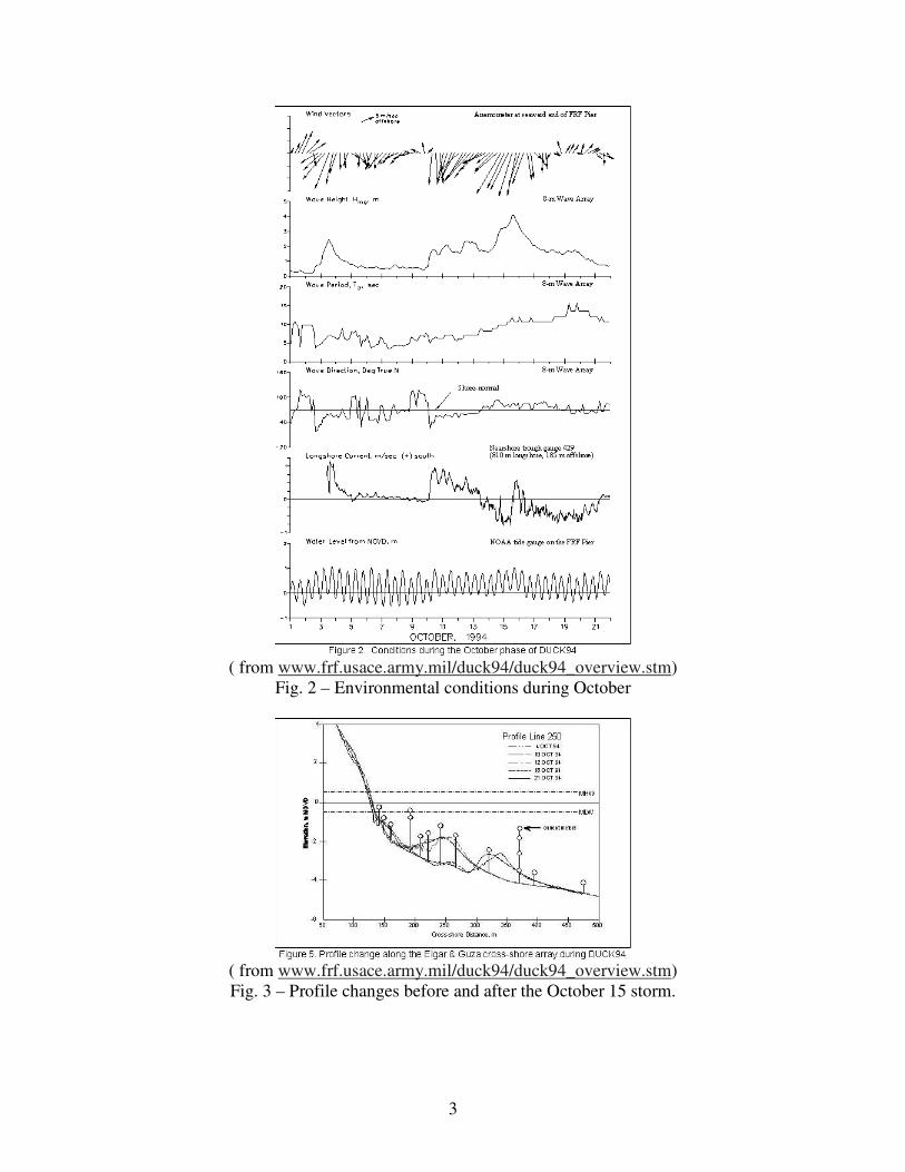
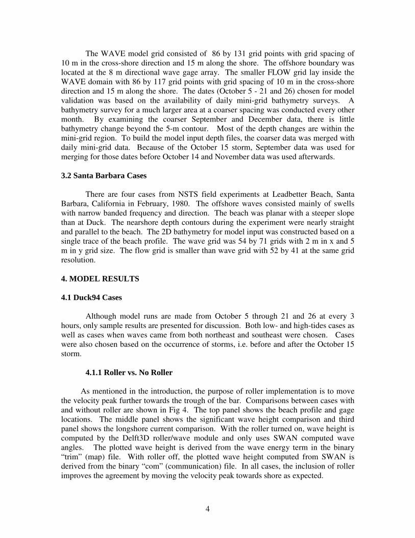
• The wave direction is still derived from an initial WAVE run. The full equations for the flow and roller model are not repeated here (Roelvink, 2003; Reniers et al., 2004). 3. FIELD DATA AND MODEL SETUP 3.1 Duck94 Cases Duck94 field experiment was conducted in August and October near the Army Corps of Engineers’ Field Research Facility pier located in Duck, North Carolina. The instrument layout is shown in Fig. 1. The so called mini-grid is marked by the box. A bathymetry survey for the mini-grid was conducted daily during the intensive study period in October. The wave, wind and tide conditions during October were shown in Fig. 2. A storm from the southeast occurred around October 15 with a peak significant wave height reaching 4 m. The beach profile was significantly changed after the storm as illustrated in Fig. 3.

( from www.frf.usace.army.mil/duck94/duck94_overview.stm)

Fig. 1- Instrument layout at Duck94.

3

( from www.frf.usace.army.mil/duck94/duck94_overview.stm)

Fig. 2 – Environmental conditions during October

( from www.frf.usace.army.mil/duck94/duck94_overview.stm) Fig. 3 – Profile changes before and after the October 15 storm.

4

The WAVE model grid consisted of 86 by 131 grid points with grid spacing of 10 m in the cross-shore direction and 15 m along the shore. The offshore boundary was located at the 8 m directional wave gage array. The smaller FLOW grid lay inside the WAVE domain with 86 by 117 grid points with grid spacing of 10 m in the cross-shore direction and 15 m along the shore. The dates (October 5 - 21 and 26) chosen for model validation was based on the availability of daily mini-grid bathymetry surveys. A bathymetry survey for a much larger area at a coarser spacing was conducted every other month. By examining the coarser September and December data, there is little bathymetry change beyond the 5-m contour. Most of the depth changes are within the mini-grid region. To build the model input depth files, the coarser data was merged with daily mini-grid data. Because of the October 15 storm, September data was used for merging for those dates before October 14 and November data was used afterwards. 3.2 Santa Barbara Cases There are four cases from NSTS field experiments at Leadbetter Beach, Santa Barbara, California in February, 1980. The offshore waves consisted mainly of swells with narrow banded frequency and direction. The beach was planar with a steeper slope than at Duck. The nearshore depth contours during the experiment were nearly straight and parallel to the beach. The 2D bathymetry for model input was constructed based on a single trace of the beach profile. The wave grid was 54 by 71 grids with 2 m in x and 5 m in y grid size. The flow grid is smaller than wave grid with 52 by 41 at the same grid resolution. 4. MODEL RESULTS 4.1 Duck94 Cases Although model runs are made from October 5 through 21 and 26 at every 3 hours, only sample results are presented for discussion. Both low- and high-tides cases as well as cases when waves came from both northeast and southeast were chosen. Cases were also chosen based on the occurrence of storms, i.e. before and after the October 15 storm. 4.1.1 Roller vs. No Roller

As mentioned in the introduction, the purpose of roller implementation is to move the velocity peak further towards the trough of the bar. Comparisons between cases with and without roller are shown in Fig 4. The top panel shows the beach profile and gage locations. The middle panel shows the significant wave height comparison and third panel shows the longshore current comparison. With the roller turned on, wave height is computed by the Delft3D roller/wave module and only uses SWAN computed wave angles. The plotted wave height is derived from the wave energy term in the binary “trim” (map) file. With roller off, the plotted wave height computed from SWAN is derived from the binary “com” (communication) file. In all cases, the inclusion of roller improves the agreement by moving the velocity peak towards shore as expected.

5

(a) Oct. 10, EST 1600

(b) Oct. 12, EST 1300

6

(c) Oct. 19, EST 1000

(d) Oct. 26, EST 2200

Fig. 4 – Comparisons between cases with and without roller. EST represents Eastern Standard Time. 4.1.2 Breaking Dissipation Formulation

In Delft3D, the use of new features which have not been made to be a standard version is specified under the data group “additional parameters”. Keyword and its corresponding value are entered. One available keyword is Gamdis for specifying the gamma value, i.e. the significant wave height to depth ratio associated with depth-induced breaking. In the present version, if one uses the stationary roller model, the Baldock dissipation model is used, for which Gamdis is set at the default value of 0.55. If one sets the Gamdis keyword at -1, variable gamma value is used using Ruessink's

7

formulation (Ruessink et al., 2003). The comparisons between Baldock and Ruessink breaking dissipation formulation are shown in Fig. 5. In general, the Ruessink’s formulation produces better agreement in longshore current with a narrower velocity distribution profile, i.e. smaller offshore values and more peaked at velocity maximum. The shape of the velocity profile also depends on the empirical constant of turbulent eddy viscosity associated with mixing (Battjes, 1975). The default value is 1. The same value is also used by NSSM (Hsu, et al, 2000). Note that the background horizontal eddy viscosity as defined in the data group “physical parameters” is not used when roller is turned on.

(a) Oct. 10, EST 1600

(b) Oct. 12, EST 1300

8

(c) Oct. 19, EST 1000

(d) Oct. 26, EST 2200

Fig. 5 – Comparison of breaking dissipation formulations.

4.1.3 Breaker Delay

An optional feature called 'breaker delay’ is available through the keyword F_lam with a value -2, the description is given in Roelvink et al (2000). It applies a weighted averaging of the depth used in the wave dissipation model, to a number of wavelengths seaward. The comparisons between cases with and without breaker delay are shown in Fig. 6. Except for Oct. 26, all other cases show a slight movement of peak velocity towards trough. For case of Oct. 26, the improvement is negligible.

9

(a) Oct. 10, EST 1600

(b) Oct. 12, EST 1300

10

(c) Oct. 19, EST 1000

(d) Oct. 26, EST 2200

Fig. 6 – Comparison between cases with and without applying breaker delay

4.1.4 Turn off the Roller Stress at very shallow water In very shallow water, say depth less than 0.5 m, Delft3D occasionally generates large currents, due to unrealistic roller or wave forces. In Delft3D, roller stress is turned off for depth shallower than 2 times the specified threshold depth, which is used to define the depth above which a grid cell is considered to be wet. Designated as dryflc under the data group “numerical parameters”, its default value is 0.1 m. From our experience, the value of dryflc needs to be slightly increased to avoid unrealistically large current at shallow depth. The impact of the selection of dryflc is illustrated in Fig. 7. The significant reduction of the second peak near shoreline at dryflc = 0.2 m, i.e. roller stress

11

turned off at 0.4 m, is very clear in case (a). In the other cases, the reduction is small. It is important to note that the selection of dryflc does not have much impact to the rest of the velocity distribution away from the more shallow water.

(a) Oct. 10, EST 1600

(b) Oct. 12, EST 1300

12

(c) Oct. 19, EST 1000

(d) Oct. 26, EST 2200

Fig. 7 – The effects of turning off roller stress at very shallow water.

4.1.5 The Effect of Bottom Friction Selection For 2-D simulations, three roughness formulations, i.e. Manning, White-Colebrook (W-C) and Chezy, can be selected at the roughness menu under the data group “physical parameters”. By definition, the bottom friction coefficient, Cf, is related to Chezy roughness coefficient C by

2/ CgC f = (1) where g is the acceleration due to gravity. The default Chezy formulation is for specifying a constant Chezy value for the whole domain, i.e. no depth dependency. For Manning formulation, the Chezy coefficient is related to the Manning roughness coefficient, n, as,

13

nhC /6/1= (2) where h is the water depth. For W-C formulation, one needs to specify the equivalent geometrical roughness of Nikuradse, ks. The Chezy coefficient is calculated from: ( )skhC /12log18 ⋅⋅= (3) In Morris’s investigation (2001), he chose the W-C formulation. The optimal value of ks based on Duck runs was found to be 0.003 m for the barred beach corresponding cross-shore averaged Cf about 0.002. He also reported that the optimal value of ks based on planar beach at Torrey Pines and Santa Barbra beaches was 0.009 m with a corresponding averaged Cf at 0.004. As for the Manning formulation, the suggested default value for n is 0.02 in the Delft3D FLOW manual. Grunnet et al. (2004) uses a value of 0.0225 for a barrier island sediment study using Delft3D. The default value for Chezy formulation is 65, equivalent to a bottom friction coefficient of 0.0023. The depth dependence of both Manning and W-C formulations is illustrated in Fig. 8 for a linear beach. Both formulations show a weak dependence of depth until depth is very shallow, say 0.5 m. It is noted that the curve with Manning n at 0.02 and W-C ks at 0.009 are very similar. The averaged Cf value will depend on the shape and depth of the real beach profile. For the linear beach in Fig. 8, the corresponding cross-shore averaged Cf value for n = 2 is about 0.0028, and is about 0.0024 for ks at 0.009.

Fig. 8 – Depth dependence of bottom friction coefficient, Cf , for Manning and White-Colebrook roughness formulations.

14

To evaluate the effects of bottom friction dependence, comparison plots are presented in Fig. 9. The figures show that Morris’ selection of W-C at ks = 0.003 based on DELILAH field data still works reasonably well for Duck94. The cases using default Chezy C at 65 tend to over-predict the velocity peaks whereas the cases using C at 55 (equivalent to Cf at 0.0032) match the data slightly better. The Manning formulation at n = 0.02 works well.

(a) Oct. 10, EST 1600

(b) Oct. 12, EST 1300

15

(c) Oct. 19, EST 1000

(d) Oct. 26, EST 2200

Fig. 9 – The comparison of bottom friction selections To study the impact of bottom friction further, 64 out of the computed 116 cases of Duck94 data were used for statistical computation. The cases with rip current or big eddies are not appropriate for evaluating the effect of bottom friction, and therefore were not included. The eddy formation is associated with the instability at the southern boundary when waves are coming from southeast. For Neumann boundary conditions to work well, the bathymetry longshore near the side boundaries of SWAN needs to be uniform. More than 20 grid spaces of alongshore uniform depth values are provided for the northern boundary whereas only 5 were provided in the southern boundary. It turns out that 5 grid spaces are not enough for Neumann boundary condition to work well. As a rule of thumb, more than 15 grid spaces should be used in both boundaries in any future setup. It is useful to set a few side boundary grid cells in the flow bathymetry to the same depth as SWAN to achieve further smooth transition.

16

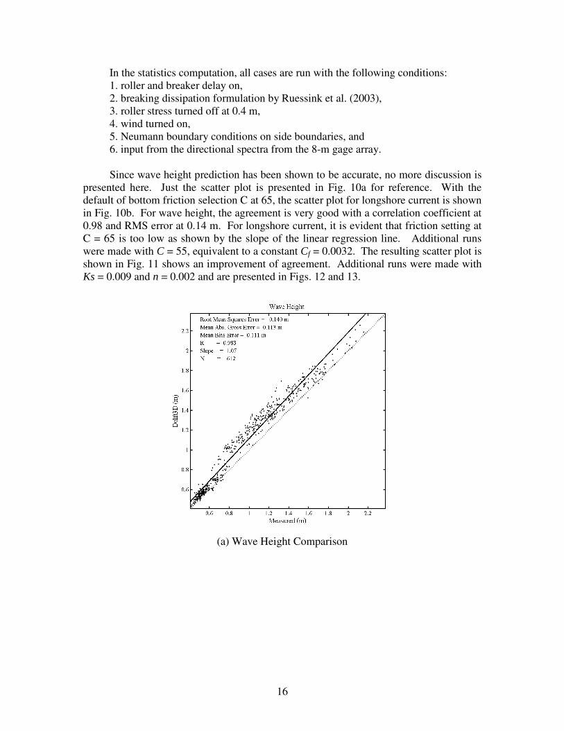
In the statistics computation, all cases are run with the following conditions: 1. roller and breaker delay on, 2. breaking dissipation formulation by Ruessink et al. (2003), 3. roller stress turned off at 0.4 m, 4. wind turned on, 5. Neumann boundary conditions on side boundaries, and 6. input from the directional spectra from the 8-m gage array. Since wave height prediction has been shown to be accurate, no more discussion is

presented here. Just the scatter plot is presented in Fig. 10a for reference. With the default of bottom friction selection C at 65, the scatter plot for longshore current is shown in Fig. 10b. For wave height, the agreement is very good with a correlation coefficient at 0.98 and RMS error at 0.14 m. For longshore current, it is evident that friction setting at C = 65 is too low as shown by the slope of the linear regression line. Additional runs were made with C = 55, equivalent to a constant Cf = 0.0032. The resulting scatter plot is shown in Fig. 11 shows an improvement of agreement. Additional runs were made with Ks = 0.009 and n = 0.002 and are presented in Figs. 12 and 13.

(a) Wave Height Comparison

17

(b) Longshore Current Comparison

Fig. 10 – Scatter plots for (a) wave height and (b) longshore current using default Chezy formulation with C = 65. R is linear correlation coefficient; Slope is the slope of the linear regression line (solid line). N is the number of observations.

Fig. 11 – Scatter plot for longshore current excluding cases with eddy formation using Chezy with C = 55.

18

Fig. 12 - Scatter plot for longshore current excluding cases with eddy formation using W-C formulation at ks = 0.003.

Fig. 13 - Scatter plot for longshore current excluding cases with eddy formation using Manning formulation at n = 0.002.

The skill statistics of four different bottom friction formulations are summarized in Table 1. In addition to root mean squares error (RMSE), mean absolute gross error (MAGE) and mean bias error (MBE) are also listed. The model performance at default

19

Chezy C = 65 (equivalent to Cf at 0.0023) is worse that C =55 (equivalent to Cf at 0.0032), indicating the default bottom friction is slightly too low. This is consistent with previous field measurements of bottom friction at Duck (Whitford and Thornton, 1996). Overall, the performance of all three different formulations is very similar. The Manning formulation with n = 0.02 and Chezy formulation with C=55 produce better performance. Table 1 – Skill statistics for different bottom friction selections RMSE(m/s) MAGE (m/s) MBE (m/s) R Slope N Chezy C=65 0.18 0.13 0.024 0.914 1.12 533 Chezy C =55 0.14 0.10 -0.009 0.918 0.9 533 W-C ks =0.003 0.20 0.15 0.041 0.912 1.20 533 Manning n=0.02 0.14 0.11 0.002 0.919 0.95 533 The statistics of RMS error is influenced by the large number of low velocity data points. Fig. 14 shows the scatter plot under Chezy at C = 55 where no measured data under 0.1 m are included. The RMS value is increased as expected. The skill statistics of data excluded velocity below 0.1 m/s is shown in Table 2.

Fig. 14 – Scatter plot for longshore current excluding measured velocity less than 0.1 m/s using Manning formulation at n = 0.02.

20

Table 2 – Skill statistics for different bottom friction selections excluding measured velocity less than 0.1 m/s. RMSE(m) MAGE (m/s) MBE (m/s) R Slope N Chezy C=65 0.2 0.16 0.052 0.914 1.09 374 Chezy C =55 0.16 0.12 0.001 0.918 0.87 374 W-C ks =0.003 0.23 0.18 0.076 0.91 1.17 374 Manning n=0.02 0.16 0.13 0.016 0.917 0.93 374 4.2 Santa Barbara Unlike the barred beach at Duck, Santa Barbara has planar and steeper beach, and therefore is useful in testing the robustness of Delft3D features. Since the four available cases are similar in wave input and beach profile, only one case, i.e. Feb. 03, 1980, is presented. 4.2.1 Roller vs. No Roller Comparison of results with and without roller is shown in Fig. 15. Similarly to Duck, the case with roller gives better longshore current results. The sharp decay of the longshore current at the beach for the roller case is partly because the roller stress was turned off at 0.4 m. The case was run with the Manning formulation at n = 0.015.

Fig. 15 – Comparison between with and without roller.

21

4.2.2 Breaking Dissipation formulation The comparison of default and Ruessink formulations is presented in Fig. 16.

The Ruessink approach also gives better results for a planar beach.

Fig. 16– Comparison between different breaking dissipation formulations.

4.2.3 Breaker Delay The comparison between that which was with and without breaker delay is

presented in Fig. 17 The breaker delay produces worse agreement in longshore current.

Fig. 17– Comparison between with and without breaker delay.

22

4.2.4 The Effect of Bottom Friction Selection

The comparison between four different bottom friction selections, Chezy with C = 65, C = 55 and Manning with n = 0.0.015 and n = 0.02, is presented in Fig. 18 Compared with Duck results, it is evident that sensitivity to the empirical bottom friction value is much higher at the steeper Santa Barbara beach. Unlike the Duck94 cases, the default choice of Chezy with C = 65 (Cf = 0.0023) produces better agreement than C = 55 (Cf = 0.0032). In Morris’ investigation, the optimal value (ks = 0.009 corresponding averaged Cf at 0.004) required at Santa Barbara is twice higher than at Duck (ks = 0.003 corresponding averaged Cf at 0.002). So our trend is reverse to Morris findings. It is difficult to isolate what caused the difference between these two different versions of Delft3D, because a lot of improvements have been implemented. One reason for the difference may be associated with the different breaking dissipation formulation used.

Fig. 18– Comparison of Delft3D results between different bottom friction selections. 5. SUMMARY AND CONCLUSIONS

The main focus of this investigation is to examine the effects of bottom frictions selection. Both Duck94 and NSTS Santa Barbara data were used for evaluating Delft3D performance. All three bottom friction formulations, i.e. Chezy, White-Colebrook and Manning, were evaluated and all produced good longshore current results, if proper empirical constant is used. The RMS error for longshore current is about 0.2 m/s. Over barred beach at Duck, the optimal values are n = 0.02 (Manning) and C = 55 (Chezy, Cf = 0.0032). Over the steeper planar beach at Santa Barbara, the optimal values are Manning with n = 0.015 and Chezy with C = 65 (Cf = 0.0023). The difference in optimal values (i.e. Cf from 0.0023 to 0.0032) between different beaches is therefore not as high as indicated by a previous study (i.e. Cf from 0.002 to 0.004, Morris, 2003). This difference may be attributed to the difference in breaking dissipation formulations used. Further evaluation/validation for some other beaches is needed to provide a general guideline for the selecting optimal values.

Many other Delft3D model parameters and options were also evaluated. The

inclusion of roller is shown to improve the longshore current prediction for both Duck and Santa Barbara beaches. As the selection of breaking dissipation formulation, the

23

Ruessink formulation with variable gamma value (significant wave height to depth ratio) provides better results than the default setting. The optional breaker delay slightly improves the longshore current prediction at Duck, but it produces a worse result at Santa Barbara beach. To avoid spuriously high currents at very shallow depth, roller stress is recommended to be turned off at shallow depth, say 0.4 m. In general, Delft3D has shown to be robust and accurate in predicting nearshore flows. ACKNOWLEDEMENTS The authors wish to thank Dr. Edward Thornton, Naval Postgraduate School, Dr. Robert Guza, Scripps Institution of Oceanography, Dr. Steve Elgar, Woods Hole Oceanographic Institute and Dr. Chuck Long, Army Field Research Facility for providing the NSTS and DUCK94 data sets. This work was sponsored by ONR under project: Development of an AUV-Fed Nearshore Nowcasting System RTP, and by SPAWAR PMW 150 under project: Nearshore wave and surf prediction. REFERENCES Battjes, J.A.,1975: Modeling of turbulence in the surfzone, Sym. On modeling

techniques, Am. Soc. of Civ. Eng., San Francisco, CA. Dykes, J. D., Y. L. Hsu, J. M. Kaihatu, 2003: Application of Delft3D in the Nearshore

Zone, Proc. 5th AMS Coastal Conf., Seattle, Washington, 57-61. Hsu, Y.L., T.R. Mettlach and M.D. Marshall, 2002: Validation test report for the Navy

Standard Surf Model, NRL formal report: FR/7322-02-10008. Grunnet, N.M., D-J.R. Walstra, B.G. Ruessink, 2004: Process-based modeling of a

shoreface nourishment, Coastal Eng.,51,581-607. Morris, B.J., 2001: Nearshore wave and current dynamics, Ph. D. Dissertation, Naval

Postgraduate School. Ris, R.C., N. Booij, and L.H. Holthuijsen, 1999: “A Third Generation Wave Model for

Coastal Region, Part II: Verification,”, J. Geophys. Res. 104(C4), 7667-7681. Reniers, A.J.H.M.,A.R. Van Dongeren, J.A. Battjes, and E. B. Thornton, 2002, Linear

modeling of infra-gravity waves during Delilah, J. Geophys. Res., 107(C10), 3137. Roelvink, J.A., 2003, Implementation of roller model, draft Delft3D manual, Delft

Hydraulics Institute. Roelvink J.A. and D.-J. Walstra, 2004: Keeping it simple by using complex models, The

6th Int. Conf. on Hydroscience and Engineering , May 30-June3, Brisbane, Australia.

24

Roelvink, J.A., T.J.G.P. Meijer, K. Houwman, R. Bakker and R. Spanhoff, 1995: Field validation and application of a coastal profile model. Proc. Coastal Dynamics '95, Gdansk, ASCE, New York, pp. 818-828.

Ruessink, B.G., J.R. Miles, F. Feddersen, R.T. Guza and S. Elgar, 2001: Modeling the alongshore current on barred beaches, J. Geophys. Res., 106(C10), 22451-22463. Ruessink, B.G., D.J.R. Walstra and H.N. Southgate, 2003: Calibration and verification of

a parametric wave model on barred beaches, Coast. Eng., 48, 139-149. Whitford, D.J. and E.B. Thornton, 1996: Bed shear stress coefficients for longshore

currents over a barred profile, Coast. Eng., 27, 243-262.