Sept/Oct 2003 3

ARRL Technical Advisor41 Glenwood RdAndover, MA 01810-6250ai1h@arrl.net

Evaluation of Antenna Tunersand Baluns–An Update

By Frank Witt, AI1H

How to have high confidence in your measurements.

In a two-part article in April and May 1995 QST,1 Idescribed a simple method for evaluating antennatuners. Application to the evaluation of baluns was de-

scribed the following year.2 The method involves a resis-tance-load box and a low-power analyzer, and it worksequally well for evaluating the performance of equipmentwith balanced as well as unbalanced loads. A simple ex-tension was described that allows the equipment evalua-tion with complex-impedance loads as well.

Amateurs around the world have since used the method,which has been dubbed the “indirect method,” the “AI1Hmethod” and the “Witt method.” It provides—at moderatecost—a simple means for evaluating antenna tuners andbaluns. The method was used to evaluate four antenna tun-ers for a Product Review in March 1997 QST.3

Most hams had been ignorant about the performanceof their antenna tuners. They only knew the circuits were

1Notes appear on page 14.

lossy when they got very hot or when a component failed(if running high power). QRPers had no way of knowingwhether or not their antenna tuners handicapped them.Some manufacturers’ claims for their antenna tuners were(and still are) unreliable, and that is being kind. Muchlight was shed on this matter by the programs written byDean Straw, N6BV, TLA and its successor TLW,4 whichcompute antenna-tuner performance. The indirect methodcomplements this analysis tool by providing a very acces-sible measurement tool.

From the source in Note 1 (May 1995, page 37): “Thisnew application of low-power SWR testers is a demandingone, since the accuracy must be excellent for valid results.Perhaps we will see even more accurate SWR testers in thefuture, and maybe antenna tuner manufacturers will beinspired to improve their designs.” That day has arrived.Improved SWR analyzers and antenna tuners5 are nowavailable.

The purpose of this article is to show how measurementinstruments that are now available provide improved ac-curacy for the simple characterization of antenna tunersand baluns. It summarizes a better understanding of anyinherent limitations of the evaluation method. Finally, itprovides a comparison with other measurement methods.

4 Sept/Oct 2003

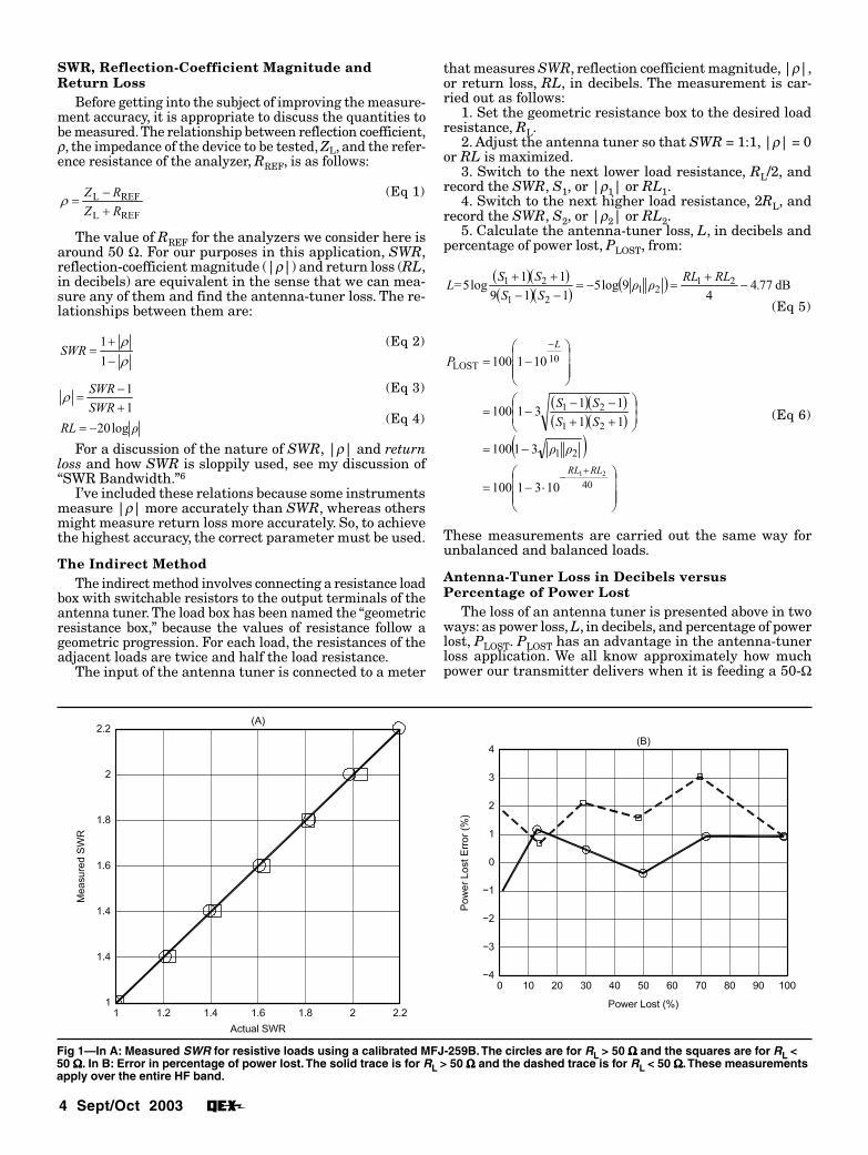
Fig 1—In A: Measured SWR for resistive loads using a calibrated MFJ-259B. The circles are for RL > 50 ΩΩΩΩΩ and the squares are for RL <50 ΩΩΩΩΩ. In B: Error in percentage of power lost. The solid trace is for RL > 50 ΩΩΩΩΩ and the dashed trace is for RL < 50 ΩΩΩΩΩ. These measurementsapply over the entire HF band.

SWR, Reflection-Coefficient Magnitude andReturn Loss

Before getting into the subject of improving the measure-ment accuracy, it is appropriate to discuss the quantities tobe measured. The relationship between reflection coefficient,ρ, the impedance of the device to be tested, ZL, and the refer-ence resistance of the analyzer, RREF, is as follows:

REFL

REFL

RZ

RZ

+−

=ρ(Eq 1)

The value of RREF for the analyzers we consider here isaround 50 Ω. For our purposes in this application, SWR,reflection-coefficient magnitude (|ρ|) and return loss (RL,in decibels) are equivalent in the sense that we can mea-sure any of them and find the antenna-tuner loss. The re-lationships between them are:

ρρ

−+

=1

1SWR

(Eq 2)

1

1

+−

=SWR

SWRρ(Eq 3)

ρRL log20−=(Eq 4)

For a discussion of the nature of SWR, |ρ| and returnloss and how SWR is sloppily used, see my discussion of“SWR Bandwidth.”6

I’ve included these relations because some instrumentsmeasure |ρ| more accurately than SWR, whereas othersmight measure return loss more accurately. So, to achievethe highest accuracy, the correct parameter must be used.

The Indirect MethodThe indirect method involves connecting a resistance load

box with switchable resistors to the output terminals of theantenna tuner. The load box has been named the “geometricresistance box,” because the values of resistance follow ageometric progression. For each load, the resistances of theadjacent loads are twice and half the load resistance.

The input of the antenna tuner is connected to a meter

that measures SWR, reflection coefficient magnitude, |ρ|,or return loss, RL, in decibels. The measurement is car-ried out as follows:

1. Set the geometric resistance box to the desired loadresistance, RL.

2. Adjust the antenna tuner so that SWR = 1:1, |ρ| = 0or RL is maximized.

3. Switch to the next lower load resistance, RL/2, andrecord the SWR, S1, or |ρ1| or RL1.

4. Switch to the next higher load resistance, 2RL, andrecord the SWR, S2, or |ρ2| or RL2.

5. Calculate the antenna-tuner loss, L, in decibels andpercentage of power lost, PLOST, from:

( )( )( )( )

( ) dB 7744

9log5119

11log5 21

2121

21 .RLRLρρ

SS

SSL= −

+=−=

−−++

(Eq 5)

( )( )( )( )

( )

⋅−=

−=

++−−

−=

−=

+−

−

40

21

21

21

10LOST

21

1031100

31100

11

1131100

101100

RLRL

L

ρρ

SS

SS

P

(Eq 6)

These measurements are carried out the same way forunbalanced and balanced loads.

Antenna-Tuner Loss in Decibels versusPercentage of Power Lost

The loss of an antenna tuner is presented above in twoways: as power loss, L, in decibels, and percentage of powerlost, PLOST. PLOST has an advantage in the antenna-tunerloss application. We all know approximately how muchpower our transmitter delivers when it is feeding a 50-Ω

Sept/Oct 2003 5

Fig 2 — In A: Measured reflection-coefficient magnitude for resistive loads using a calibrated MFJ-259B. The circles are for RL > 50 ΩΩΩΩΩand the squares are for RL < 50 ΩΩΩΩΩ. In B: Error in percentage of power lost. The solid trace is for RL > 50 ΩΩΩΩΩ and the dashed trace is for RL< 50 ΩΩΩΩΩ. These measurements apply over the entire HF band.

load. What we want to know is how much of that power isbeing absorbed or radiated by the antenna tuner and notreaching the antenna system. Percentage of power lost tellsus this directly. For example, a kilowatt transmitter feed-ing an antenna tuner with a 20% of power lost figure meansthat 200 W are lost in the antenna tuner. Most of thatpower is usually heating components in the tuner.

On the other hand, if the loss is expressed in decibels,we must make a mental translation to percentage of powerlost in order to know what is happening. Some familiardecibel-loss quantities are 0, 1, 3 and 10 dB, which equateto 0%, 21%, 50% and 90% of the power lost in the antennatuner, respectively. Other quantities of decibel loss are farless familiar to most of us. So, the preferred loss-charac-terization method is percentage of power lost. It is inter-

esting to notice from Eq 6 that percentage of power lost islinearly related to the geometric mean of the reflection-coefficient magnitude readings.

Accuracy of the AnalyzersMFJ-259B

When I first discovered the indirect method, I used low-power SWR testers. These were the Autek Research ModelRA1 and the MFJ Model MFJ-259. These units displayedSWR, so the SWR reading was used for loss calculationsusing Eqs 5 and 6. These instruments do not display |ρ|,although it is the basic quantity measured. SWR is calcu-lated internally from the value of |ρ|. This calculation isa source of error. Fortunately, some newer instruments

Fig 3 — In A: Measured return loss for resistive loads using a calibrated MFJ-259B. The circles are for RL > 50 ΩΩΩΩΩ and the squares arefor RL < 50 ΩΩΩΩΩ. In B: Error in percentage of power lost. The solid trace is for RL > 50 ΩΩΩΩΩ and the dashed trace is for RL < 50 ΩΩΩΩΩ. Thesemeasurements apply over the entire HF band.

6 Sept/Oct 2003

Fig 5—Resolution of the MFJ-259B for SWR. In A: The values of SWR that may be displayed. In B: The resolution over the 0 to 100%percentage of power lost range.

Fig 4—Values of reflection-coefficient magnitude that can bedisplayed by the MFJ-259B. This results in a resolution capabilityfor percentage of power lost of 0.75%. Notice the linearrelationship between percentage of power lost and |ρρρρρ|.

display |ρ| and return loss directly. Further, SWR, |ρ|and return loss are displayed on a LCD, which is easier toread reliably than an analog meter. An instrument formeasuring the loss of antenna tuners is the MFJ-259B,the successor to the MFJ-259. Some features of other can-didates for this application are discussed later in the ar-ticle, but here we will primarily answer the question ofwhether or not the MFJ-259B will perform adequately inthis application.

Although the MFJ-259B impedance analyzer measuresmany properties of the unknown connected to its termi-nals, we will focus here on the antenna-tuner evaluationapplication. It fared well compared with similar units in arecent review.7 As indicated above, antenna-tuner loss canbe determined from SWR, |ρ| or return loss. The accuracyof the MFJ-259B can be improved through a calibrationprocedure, which is described below. SWR, |ρ| and returnloss were measured. The date on the unit tested is 1998and the software version is 2.02. The measurement fre-quency was 1.8 MHz and the load resistors were 1/4-W, 1%metal-film resistors with very short leads. These resistorsare the “standard” for the evaluation of the analyzer. Testsconfirmed that the 1.8-MHz data applies over the entireHF band. The dc values for the load resistors were mea-sured with a digital multimeter. I have made measure-ments using complex-impedance loads that show similaraccuracy. This is important, because the impedances seenby the MFJ-259B in this application are complex.

The results are shown in Figs 1, 2 and 3 for SWR, |ρ|and return loss, respectively.8 Notice that separate datapoints and traces are obtained for load resistances aboveand below RREF. Although the “measured versus actual”plots are interesting, the useful information is containedin the graphs. They show the error in percentage of powerlost versus the actual percentage of power lost. Thesegraphs use Eq 6 to find the percentage of power lost, butmake the assumption that |ρ1| and |ρ2| are the same.The “true” percentage of power lost is assumed to be thatcalculated from the measured dc resistance values. Theerror is found by subtracting this true percentage of powerlost from that calculated using measurements from theMFJ-259B. For both SWR and |ρ|, the errors are less thanabout 3% for percentage of power losses from 0 to 100%.

The error for return loss is around 8%, however. These dif-ferences arise from deficiencies in the algorithm that con-verts the basic |ρ| measurement into return loss and thepoor resolution of return-loss measurements in part of thedesired region, which is discussed later.

For all calculations, it was assumed that the referenceresistance, RREF, for this particular MFJ-259B is 50.1 Ω.This is the value of RREF that gives the lowest mean-squareerror (0.77%) for percentage of power losses from 0 to 100%.RREF is nominally 50 Ω, but this method of finding the ac-tual value provides a better evaluation of the MFJ-259B.

Measurement ResolutionA measuring instrument is limited by its resolution.

Even if the accuracy is perfect, the ability to display theresult is controlled by its resolution. The display on theLCD for each parameter measured limits its resolution.

Sept/Oct 2003 7

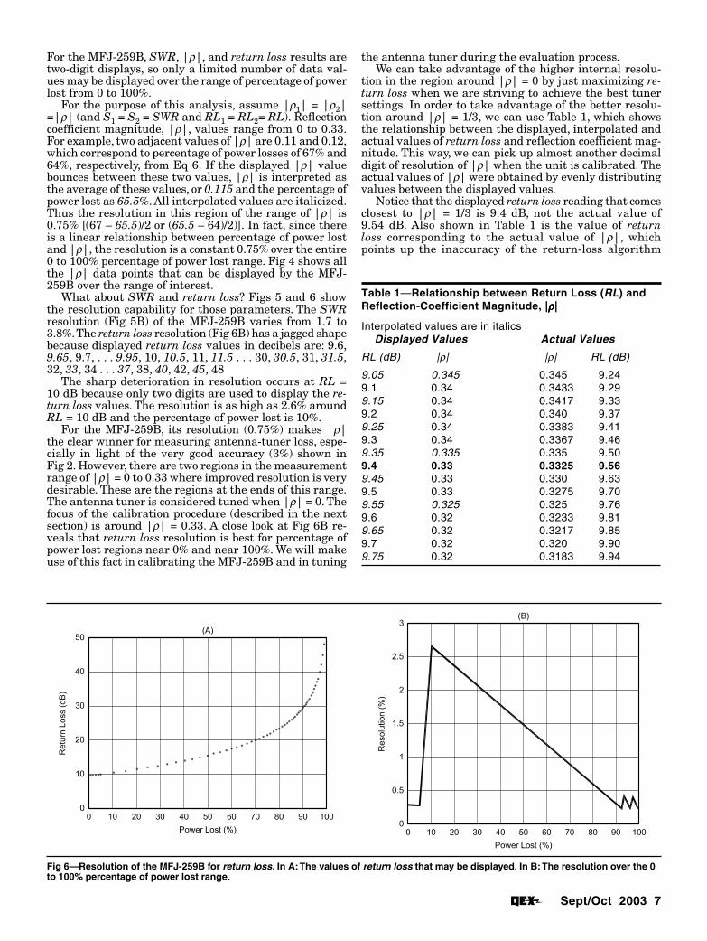
Fig 6—Resolution of the MFJ-259B for return loss. In A: The values of return loss that may be displayed. In B: The resolution over the 0to 100% percentage of power lost range.

For the MFJ-259B, SWR, |ρ|, and return loss results aretwo-digit displays, so only a limited number of data val-ues may be displayed over the range of percentage of powerlost from 0 to 100%.

For the purpose of this analysis, assume |ρ1| = |ρ2|=|ρ| (and S1 = S2 = SWR and RL1 = RL2= RL). Reflectioncoefficient magnitude, |ρ|, values range from 0 to 0.33.For example, two adjacent values of |ρ| are 0.11 and 0.12,which correspond to percentage of power losses of 67% and64%, respectively, from Eq 6. If the displayed |ρ| valuebounces between these two values, |ρ| is interpreted asthe average of these values, or 0.115 and the percentage ofpower lost as 65.5%. All interpolated values are italicized.Thus the resolution in this region of the range of |ρ| is0.75% [(67 – 65.5)/2 or (65.5 – 64)/2)]. In fact, since thereis a linear relationship between percentage of power lostand |ρ|, the resolution is a constant 0.75% over the entire0 to 100% percentage of power lost range. Fig 4 shows allthe |ρ| data points that can be displayed by the MFJ-259B over the range of interest.

What about SWR and return loss? Figs 5 and 6 showthe resolution capability for those parameters. The SWRresolution (Fig 5B) of the MFJ-259B varies from 1.7 to3.8%. The return loss resolution (Fig 6B) has a jagged shapebecause displayed return loss values in decibels are: 9.6,9.65, 9.7, . . . 9.95, 10, 10.5, 11, 11.5 . . . 30, 30.5, 31, 31.5,32, 33, 34 . . . 37, 38, 40, 42, 45, 48

The sharp deterioration in resolution occurs at RL =10 dB because only two digits are used to display the re-turn loss values. The resolution is as high as 2.6% aroundRL = 10 dB and the percentage of power lost is 10%.

For the MFJ-259B, its resolution (0.75%) makes |ρ|the clear winner for measuring antenna-tuner loss, espe-cially in light of the very good accuracy (3%) shown inFig 2. However, there are two regions in the measurementrange of |ρ| = 0 to 0.33 where improved resolution is verydesirable. These are the regions at the ends of this range.The antenna tuner is considered tuned when |ρ| = 0. Thefocus of the calibration procedure (described in the nextsection) is around |ρ| = 0.33. A close look at Fig 6B re-veals that return loss resolution is best for percentage ofpower lost regions near 0% and near 100%. We will makeuse of this fact in calibrating the MFJ-259B and in tuning

the antenna tuner during the evaluation process.We can take advantage of the higher internal resolu-

tion in the region around |ρ| = 0 by just maximizing re-turn loss when we are striving to achieve the best tunersettings. In order to take advantage of the better resolu-tion around |ρ| = 1/3, we can use Table 1, which showsthe relationship between the displayed, interpolated andactual values of return loss and reflection coefficient mag-nitude. This way, we can pick up almost another decimaldigit of resolution of |ρ| when the unit is calibrated. Theactual values of |ρ| were obtained by evenly distributingvalues between the displayed values.

Notice that the displayed return loss reading that comesclosest to |ρ| = 1/3 is 9.4 dB, not the actual value of9.54 dB. Also shown in Table 1 is the value of returnloss corresponding to the actual value of |ρ|, whichpoints up the inaccuracy of the return-loss algorithm

Table 1—Relationship between Return Loss (RL) andReflection-Coefficient Magnitude, |ρρρρρ|

Interpolated values are in italicsDisplayed Values Actual Values

RL (dB) |ρ| |ρ| RL (dB)

9.05 0.345 0.345 9.249.1 0.34 0.3433 9.299.15 0.34 0.3417 9.339.2 0.34 0.340 9.379.25 0.34 0.3383 9.419.3 0.34 0.3367 9.469.35 0.335 0.335 9.509.4 0.33 0.3325 9.569.45 0.33 0.330 9.639.5 0.33 0.3275 9.709.55 0.325 0.325 9.769.6 0.32 0.3233 9.819.65 0.32 0.3217 9.859.7 0.32 0.320 9.909.75 0.32 0.3183 9.94

8 Sept/Oct 2003

in the MFJ-259B software.Care must be taken in the use of Table 1 for other vin-

tages of MFJ-259B software, if they exist, since the valuesmay be different. This is easy to check by confirming sev-eral readings of return loss and |ρ| in the region around|ρ| = 0.33.

MFJ-259 Calibration ProcedureI do not recommend you try this calibration process

unless you have a good reason to do so and unless you areconfident that you can do it. If the unit is in warranty, youmay void the warranty. There are risks. You could inad-vertently turn the wrong adjustment screw and really messup the instrument. Wires or circuit-board pads could bebrought into contact and damage to the unit could result.

I have found that MFJ-259B impedance analyzers as de-livered (a sample of two) have adequate accuracy for gettinga good idea of how well a particular antenna tuner performs.However, if you want to squeeze the most out of your ana-lyzer, calibration is possible and can be helpful for evaluat-ing an antenna tuner. The effectiveness of the calibrationprocess is seen in Fig 2B, where the percentage-of-power-lost error is less than 1% for power losses up to 30%. As willbe seen, the calibration is made in this region.

The basic idea is to connect known load resistances tothe unit and then adjust the proper potentiometer (andthere are several, so take care) so that the appropriatereading is correct. For our purposes, we want the LCD read-ing of SWR, |ρ| and return loss to be correct. Since |ρ| isthe fundamental measurement from which SWR and re-turn loss are calculated, calibration involves getting the|ρ| reading (which is displayed only on the LCD and noton an analog meter) to be as close to the correct value aspossible. Adjustments to calibrate other quantities suchas LCD impedance, analog-meter SWR and analog-meterimpedance are also exposed when the |ρ| calibration con-trol is made available for adjustment. These other adjust-ments need not be touched to calibrate the instrument forantenna tuner and balun evaluation.

You will need two resistive loads, 25 Ω and 100 Ω, forthe calibration. These should be 1%-tolerance resistors with

minimal parasitic inductance and capacitance, hence veryshort leads. Ideally, they should be mounted inside aPL-259 connector, but this is not essential. Quarter-watt,metal-film resistors are ideal because they fit inside thecenter conductor tube of the connector. If you have an AI1Hgeometric resistance box, the 25-Ω and 100-Ω settings pro-vide adequate test loads, since the test frequency is low,1.8 MHz. These values of resistance, 25 Ω and100 Ω, should give a |ρ| ≈ 1/3 = 0.333. From Table 1, theclosest we can come to this condition is for the return lossreading to equal 9.4 dB. Notice the row shown in bold type.

I recommend that you power the MFJ-259B from ac ifyou want the calibration to hold. This eliminates possiblechanges in calibration as the batteries age. Perform thefollowing pretest before removing the back cover of theunit.

1. Turn on the MFJ-259B, enter the “Advanced” mode bysimultaneously pushing the GATE and MODE buttons,and set the unit to display “Return Loss & ReflectionCoefficient” by depressing only the MODE button once.This provides a simultaneous display of frequency, SWR,|ρ| and return loss.

2. Set the measurement frequency to 1.8 MHz.3. Connect the 25-Ω load. Wait one hour. This assures ther-

mal stabilization of the unit.4. Switch between the 25-Ω and 100-Ω loads and observe

the values of |ρ|. If they equal 0.33, 0.335 or 0.34 forboth loads, adjustment is not necessary. If not, followthe procedure below to achieve this condition.

The calibration procedure is as follows:1. Remove the back cover by removing eight screws on the

sides of the unit. Remove the batteries. Loosen the bat-tery holder by removing two screws. Fig 7 shows anMFJ-259B with the back cover and battery holderremoved.

2. Place the battery holder to the side without disconnectingit. Be careful to not let any of the exposed contacts touchthe case or any metal parts of the MFJ-259B. You maywant to wrap it in a paper towel to help avoid problems.

3. Referring to Fig 7, adjust R53 so that for both the

Fig 7—Photograph ofMFJ-259B. Notice thelocation of R53, which isused to calibrate theunit.

Sept/Oct 2003 9

25- and 100-Ω loads the return loss = 9.4 dB. This mayrequire several iterations. I recommend using a plasticalignment screwdriver, however, this is optional. If youcannot achieve RL = 9.4 dB with both loads, adjust R53so that both readings are as close to 9.4 dB as possible.9

Other AnalyzersThe major effort in improving the accuracy of measure-

ments for antenna-tuner and balun evaluation was focusedon the MFJ-259B. This emphasis was based on the poten-tial shown by that unit in a comparison of MFJ, AEA andAutek Research analyzers. To be fair, no effort was madeto tweak the AEA and Autek Research units to optimizetheir performance for this application. Some generalobservations follow.

The measuring instrument used for the measurementsback in 1995, when the indirect measurement techniquewas discovered, was the Autek Research Model RF1 RFAnalyst. This instrument displays SWR with two-digitresolution. The unit evaluated (no serial number or firm-ware version) was “as purchased” and not calibrated forthis application. It was powered by a fresh 9 V battery.The accuracy in measuring percentage of power lost wasbetter than 2% for RL > 50 Ω; however, for RL < 50 Ω thiserror was as high as 15%. The two-digit LCD SWR displayprevents precise tuning of the antenna tuner, which leadsto a tuning error that will be discussed later.

The Model VF1 RX Analyst is a more recent offering byAutek Research. The unit evaluated (no serial number orfirmware version) was tested “as purchased.” No calibra-tion was performed. A fresh 9 V battery was installed. Forthis application, this instrument displays only SWR on athree-digit LCD display. The accuracy in measuring per-centage of power lost was better than 5%.

The AEA Model CIA-HF Complex Impedance Analyzeris another candidate for making loss measurements onantenna tuners and baluns. One unit (serial #0136, Firm-ware Revision 1.4) was evaluated. The unit was evaluated“as delivered” and was not calibrated. It was powered byan external power supply. The analyzer displays SWR andreturn loss, but not reflection coefficient magnitude. Allresults are displayed on an LCD. For most values of SWRand return loss, three significant figures are shown. Forloads > 50 Ω, the error in percentage power loss was 4% orbetter for both SWR and return loss; however, for loads< 50 Ω, the error was as much as 10%, again for both SWRand return loss. It is possible that calibration would im-prove this performance. The resolution was good (threedigits), but the instability of the readings made it impos-sible to capitalize on this feature.

It is clear from the above tests that the MFJ-259B per-formed better than the Autek Research and AEA productsfor this application. I calibrated only the MFJ-259B forthese tests. It should not be inferred that the MFJ-259B isto be preferred over the other units for general analyzerapplications. More recent units might perform better. Thesedevices will improve with time because radio amateursare becoming more discriminating and aware of their ca-pabilities. Further, the imaginative ham spirit leads us toapplications that are more demanding of these analyzers.Fortunately, such improved capabilities continue to bemade available at a reasonable cost.

Other instruments of laboratory grade could be used forthis application. The “Cadillac” would be an HP (now AgilentTechnologies) Network Analyzer. Also the HP 415-seriesStanding Wave Indicator with an amplitude-modulated sig-nal generator, a return-loss bridge and a square-law detec-tor would do a good job. The HP 415-series is a selectivevoltmeter (tuned to 1 kHz) calibrated in SWR units, which

assumes that the detector has a square-law behavior. I sus-pect that each of these will beat the MFJ-259B in precisionand resolution, although this has not been confirmed.

Other Sources of ErrorLimits of Accuracy of the Indirect Method

Every method for measuring losses in antenna tunersis subject to multiple sources of error. An analysis of errorsources for the indirect method is described below. Simi-lar analyses should be performed for competing methods.

Eqs 5 and 6 for calculating the loss in decibels and per-centage of power lost are approximations. As explained inNote 1 (QST, Apr 1995, p 33): “Through computer simula-tion of many antenna tuners using a wide range of loads, Ihave found that this method of estimating loss is accurateto within a few tenths of a decibel, assuming that the SWRtester is perfect.” In spite of this, there was lingeringhealthy skepticism about the accuracy of the indirectmethod, largely because its validity is not obvious.

I have since been sent independent mathematical analy-ses from Chris Kirk, NV1E, and Kevin Schmidt, W9CF.10

They both calculated the error inherent in the use of theindirect method by using the scattering matrix formula-tion. They determined bounds on the error, that is, theworst-case error. For a given situation, the worst-caseerror may not occur; but the error caused by the use of theindirect method will never be worse than that value. Wewill call this source of error the “method error.”

The antenna tuner will in general be matched at oneport: the input port. At the input port, the tuner isadjusted so that Zin= RREF, which is nominally 50 Ω. Theoutput impedance, Zout (when the tuner input is termi-nated in 50 Ω), will be the complex conjugate of ZL, theload impedance, only if the tuner is loss-less, but we arenot measuring loss-less tuners. The source of the error inthe indirect method is this mismatch at the output port.How large is this error?

Assuming that the antenna tuner is perfectly tuned,the loads are precise and the SWR, |ρ| or return loss mea-surements are perfect, the worst-case method error boundsin decibels and in percentage of power lost are calculatedin Eq 7 and 8 below.

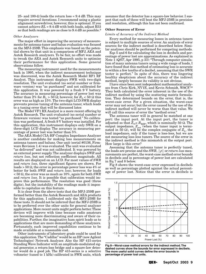
Fig 8 shows the worst-case error expressed in decibelsas well as percentage plotted against the actual percent-age of power lost. Notice that the error in decibels is

Fig 8—Worst-case method errors for the indirect method. Thedashed curves show the bounds for error expressed in decibels.The more useful solid curves define the error bounds inpercentage of power lost units.

10 Sept/Oct 2003

Fig 9—Worst-case error in percentage of power lost introduced byimperfect tuning. The dashed, solid and dotted lines show theerror bounds for |ρρρρρin| = 0.01, 0.02 and 0.03, respectively.

−

≤≤

+

−−

9

1010log5

9

108log5

1010ACTUALACTUAL LL

MethErrdB

(Eq 7)

( ) ( )

+−−≤≤

−−−

−−2

1

LOSTLOST

2

1

LOSTLOST 900

11100%900

11100P

PMethErrP

P

(Eq 8)whereLACTUAL = the actual antenna tuner loss in decibels,PLOST = percentage of power lost, andMethErrdB and MethErr% = the method error in decibels and percentage, respectively.

between –0.26 dB and +0.23 dB when the antenna tuneris absorbing most of the transmitter power. In percentageof power lost, the highest error is between –1.45% and+1.33%, and this occurs when the tuner is absorbing abouthalf of the transmitted power. This means that if perfectinstrumentation and measurement skill were appliedusing the indirect method on a tuner with 50% actual powerloss, the loss measurement would be between 48.5% and51.3%. The worst-case percentage-of-power-lost error goesto zero as the tuner loss goes to either 0 or 100%. The con-clusion is that for all practical purposes, the method errorcaused by using the indirect method is negligible.

Why is the method error so low? The error is lowbecause of the use of the geometric averaging of |ρ1| (halv-ing RL) and |ρ2| (doubling RL). See Eq 6. The process leadsto a cancellation of the large first-order error terms, andonly a much smaller second-order error term remains. Ifthe loss were calculated without using geometric averag-ing (by either halving or doubling RL), the calculated valuecould be too high by as much as 10.8% or too low by asmuch as 16%. Halving or doubling RL can yield either posi-tive or negative errors, and the error bounds are identicalfor the two cases

One can think of the antenna tuner as an impedance-transforming device. When the loss is low, the impedanceratio at the output will be seen virtually unchanged at theinput of the tuner. Hence the error is near zero for low-loss tuners. When the tuner loss is very high, the 50-Ωinput impedance of the tuned tuner is mostly made up oflossy elements within the tuner. Hence, changes in the loadimpedance do not much influence the input impedance,and the error is necessarily very low.

Incidentally, Kirk’s and Schmidt’s analyses showed thatwith one additional measurement, the error may be found,and hence subtracted. Of course, with such a low worst-case method error, such a correction is unnecessary. Othersources of error will be discussed below.

Initial Setting of Antenna TunerWhen testing an antenna tuner using the indirect

method, Step 2 says “Adjust the antenna tuner so thatSWR = 1:1, |ρ| = 0 or RL is maximized.” It is not neces-sary that RREF = 50 Ω exactly, since the tuner behaviorwill be essentially the same if it is tuned so its input im-pedance is within a few ohms of that figure. It is impor-tant, however, that the input impedance of the tuner beadjusted as close to the analyzer’s reference resistance,RREF, (usually near 50 Ω) as possible to get the mostaccurate results.

We will call the error introduced by imperfect tuningthe mistuning error. From Kevin Schmidt’s S-parameteranalysis, the mistuning error bounds in percentage ofpower lost are estimated in Eq 9 below.

The error in percentage of power lost introduced byimperfect tuning is shown in Fig 9. Notice that the effectof mistuning worsens as tuner loss increases.

With the MFJ-259B, what displayed value should be used,SWR, |ρ| or return loss? All three parameters were exam-ined in the vicinity of the desired tuned condition. Returnloss is the most sensitive indicator of the “tuned” condition.The return loss reading has to drop from 48 dB to 38 dBbefore |ρ| changes (from 0 to 0.01) and all the way to 25 dBbefore the SWR changes (from 1.0 to 1.1). This is a directresult of the two-decimal-digit display limitation for SWR,|ρ| and return loss. The return loss display has more reso-lution for this measurement and may be used. It turns out,however, that |ρ| has enough resolution to be used as well.For the MFJ-259B, SWR should not be used for this appli-

Sept/Oct 2003 11

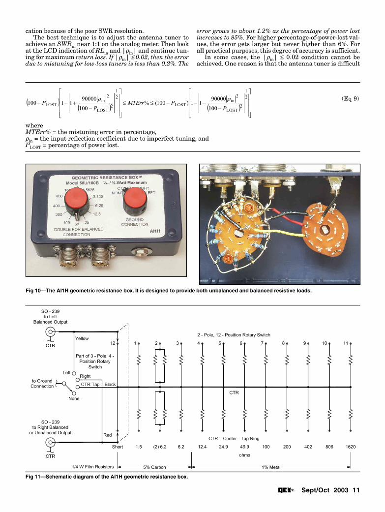
Fig 10—The AI1H geometric resistance box. It is designed to provide both unbalanced and balanced resistive loads.

Fig 11—Schematic diagram of the AI1H geometric resistance box.

cation because of the poor SWR resolution.The best technique is to adjust the antenna tuner to

achieve an SWRin near 1:1 on the analog meter. Then lookat the LCD indication of RLin and |ρin| and continue tun-ing for maximum return loss. If |ρin| ≤ 0.02, then the errordue to mistuning for low-loss tuners is less than 0.2%. The

( ) ( ) ( )

−−−−≤≤

−+−−

2

1

2LOST

2in

LOST

2

1

2LOST

2in

LOST100

9000011)100(%

100

9000011100

PPMTErr

PP

ρρ (Eq 9)

whereMTErr% = the mistuning error in percentage,ρin = the input reflection coefficient due to imperfect tuning, andPLOST = percentage of power lost.

error grows to about 1.2% as the percentage of power lostincreases to 85%. For higher percentage-of-power-lost val-ues, the error gets larger but never higher than 6%. Forall practical purposes, this degree of accuracy is sufficient.

In some cases, the |ρin| ≤ 0.02 condition cannot beachieved. One reason is that the antenna tuner is difficult

12 Sept/Oct 2003

Fig 12—Worst-case error in percentage of power lost introducedby the tolerance of the load resistors. The dashed, solid anddotted lines show the error bounds for resistors with tolerancevalues of 0.5%, 1% and 2%, respectively.

or impossible to tune for the particular load being used.Another is that the antenna tuner is made up of switchedand variable components, and precise tuning (Zin = RREF)is not possible. This problem can be overcome by first tun-ing the unit as close as possible to the |ρin| ≤ 0.02 condi-tion. Then insert a low-loss tuner with continuous-tuningcapabilities between the tuner under test and the ana-lyzer. The low-loss tuner is then tuned to achieve the |ρin|≤ 0.02 condition. The loss calculation is then the sum ofthe loss of the two tuners. Most antenna tuners will per-form well as the second tuner since they are simply trans-forming impedances near RREF to RREF.

Another potential problem is that the harmonic con-tent of the analyzer signal source is excessive. When theanalyzer is connected to a frequency-independent loadimpedance equal to RREF, the SWR, |ρ| and return lossare the same at the fundamental and at harmonics of thesource, so the |ρin| ≤ 0.02 condition is easily achieved. How-ever, when the analyzer is connected to the input of a tunedantenna tuner, the load impedance equals RREF only atthe fundamental frequency. At harmonics of the funda-mental frequency, the mismatch is huge, so harmonic sig-nal energy will disturb the reading.

The MFJ-259B contains a sufficiently clean generatorso that the |ρin| ≤ 0.02 condition is achieved. The conclu-sion is that when the signal generator has little harmoniccontent, mistuning error is a minor error contributor.

Accuracy of Load ResistanceAn advantage of the indirect method for evaluating

antenna tuners and baluns is the simple way in which theresistive loads are obtained. A geometric resistance boxprovides the load resistors and a rotary switch. The physi-cal layout is such that the parasitic inductance andcapacitance of the short connecting leads do not changewhen the load resistance is changed. The parasitic induc-tance and capacitance become a part of the tuner beingtested, and have a negligible effect on the test result.

The geometric resistance box was described in the ar-ticle of Note 1. There were two boxes, one for unbalancedmeasurements and one for balanced measurements. I havecombined these two into a single box, which is pictured inFig 10. The schematic diagram is shown in Fig 11. Noticethat most of the resistors are 1/4 W, 1% metal-film units.For the lesser values, only 5% carbon-film resistors areavailable, so the desired tolerance is achieved by selec-tion. In addition to the switched resistors, a switch isincluded for balance quality evaluation.11

The absolute value of the load resistance, RL, does notcontribute to the error. The change in tuner loss for a ±5%variation in RL is negligible. What is important, however,is the error due to imperfect ratios of adjacent loads, sinceEqs 5 and 6 are based on an assumed ratio of two. Eq 6can be generalized to include ratios other than two:

−=

−+

−=L

2121LOST 1100

1

11100

ρρρ

ρρr

rP

(Eq 10)

wherer = the geometric ratio, or the ratio of the resistances of

adjacent load resistors, and|ρL| = the load-box reflection-coefficient magnitude.

What is the error introduced when r ≠ 2 because of thetolerance of the load resistors? An analysis reveals thatthe worst-case error due to load resistance tolerance inpercentage of power lost is given by:

( ) ( )LOSTLOST 100300

4%100

300

4P

tTolErrP

t−≤≤−

(Eq 11)

wheret = the tolerance of the load resistors in percentage, andTolErr% = error due to load resistance tolerance in

percentage.A subtle factor-of-two error reduction occurs by using the

2RL and RL/2 settings in the measurement process. In effect,the tolerance of RL, the center setting causes an error in the2×RL setting, which is offset by an error of the opposite signwhen switching to RL/2. Thus for ±1% resistors, the worst-case error is only 1.33%, and this occurs for the loss-less tuner.The error from this source goes linearly to zero as the per-centage of power lost increases to 100%. See Fig 12.

If the application required it, this error could be reducedby resistor selection. The resistors cost only a few centseach. Another alternative that can essentially remove theresistor tolerance error completely is to calibrate thegeometric resistance box at dc with the aid of a precisiondigital multimeter. The various load resistors are measuredand the value of |ρL| for each RL is calculated from:

BELOWL

BELOWL

LABOVE

LABOVEL RR

RR

RR

RR

+−

⋅+−

=ρ(Eq 12)

whereRABOVE = the resistance value above RL, which is very close

to 2×RL, andRBELOW = the resistance value below RL, which is very close

to RL/2.The value of |ρL| is substituted into Eq 10 to find PLOST.

The same calibration procedure should be applied for un-balanced and balanced loads.

Human ErrorAs with any measurement process, the skill of the per-

son performing the measurement is important. Fortunately,the indirect method is simple to apply. Lots of data can beobtained in a relatively short period of time, so the datashould be processed in an orderly way. I like to use specialforms that are designed for the application. The calcula-tions are simple and can be made with a scientific calcula-tor like the one included with Microsoft Windows.

Most antenna tuners have redundant tuning adjust-ments. For example, the popular CLC T topology has three

Sept/Oct 2003 13

Fig 13—Total error bounds for all causes except for measurementinstrument inaccuracy and human error. This includes method,mistuning and load-resistance tolerance effects. It assumes that|ρρρρρin| ≤≤≤≤≤ 0.02 and the tolerance of the load resistors is 1%.

adjustments, but one can be set and the other two adjustedfor the Zin = RREF condition. This means that there are aninfinite number of settings that will achieve this condi-tion. If we make a loss measurement with a particularload at a particular frequency, then make some measure-ments with other loads and frequencies, and then try torepeat the original measurement, chances are good thatthe result will be different. One reason is that the tuneradjustments have some play, and an earlier setting is dif-ficult to duplicate. Unless great care is taken, there is ahigh likelihood that the error from this effect will be greaterthan the other errors discussed thus far, especially whenthe SWR bandwidth is small or the loss is high.

Human error is common to all methods for evaluatingantenna tuners and baluns.

Total Worst-Case ErrorFig 13 shows the bounds on error for percentage

power lost between 0 and 90% exclusive of measure-ment instrument error and human error. It includesmethod error, mistuning error and load resistance toler-ance effects. It assumes that |ρin| ≤ 0.02 and the toler-ance of the resistors is 1%. The maximum worst-case errorfrom these causes is only about 2.5%. This is entirelyacceptable for evaluating tuners and baluns.

Incidentally, these are worst-case errors. The worst-caseerrors from several causes were added up to get the totalworst-case error. The actual error will usually be muchless than the worst-case error.

Balanced Output EvaluationIn the original article describing the evaluation of

antenna tuners (Note 1), a method was presented for evalu-ating the balance quality of antenna tuners. An improvedinterpretation of the balance measurement was presentedin the balun evaluation paper12 and will be summarizedhere. This method is applicable to the evaluation of an-tenna tuners with a balanced output port.

Ideally, a balanced antenna tuner with a balanced loadwhose center tap is grounded should force equal currents(equal in magnitude and phase, but opposite in direction)to flow in each leg of the load. Let’s define these currentsas I1 and I2. If we have the ideal situation, I1 = I2. In gen-eral, the current flowing from the center tap to ground isI1 - I2 which ideally should be zero. Hence an excellentmeasure of the balance quality is “imbalance” or IMB,which is defined as:

d loadhe balancerrent in tAverage cu

p center taowing fromCurrent flIMB =

(Eq 13)

21

212II

IIIMB

+−

×=(Eq14)

Thus, if IMB is zero, the balun in the antenna tuner isdoing its job.

IMB has physical significance in an antenna system.For example, if the balanced tuner’s load is a balancedantenna fed with a balanced feed line, the common moderadiation from the feed line can be derived from IMB.

A good estimate of the imbalance for tuners withcurrent baluns can be found by connecting a balancedgeometric resistance box to the balanced output terminalsof the tuner. The switchable center tap lead is connectedto the tuner ground terminal. The imbalance test is per-formed as follows:

1. Adjust the antenna tuner for SWR = 1 or |ρ| = 0 ormaximized return loss when the center tap is floating.

2. Ground the center tap and observe the value of SWR,|ρ|, or return loss which we will call SB, |ρB| or RLB,respectively.

3. For antenna tuners with 1:1 baluns, calculate anestimate of the imbalance, IMB, from:

( )110

4

1412

20/ −=

−=−=

BRLB

BBSIMB

ρρ

(Eq15)

4. For antenna tuners with 4:1 baluns, calculate an es-timate of IMB from:

( )110

8

1814

20/ −=

−=−=

BRLB

BBSIMB

ρρ

(Eq16)

The measurement of imbalance requires no setup be-yond that required for measuring the tuner loss. It simplyrequires noting the value of SWR, |ρ| or return loss whenthe center tap of the load is grounded. Although Eqs 15and 16 are most accurate for current baluns, they may beused for voltage baluns as well.

Comparison of the Direct and Indirect MethodsThe direct method for determining antenna tuner loss

is, in concept, very straightforward, but can be done in avariety of ways. The best accuracy can be achieved with alaboratory-grade network analyzer. This test equipmenthas a built in signal source, a calibrated “standard”attenuator, which operates at a fixed frequency, and adetector. The device under test, in our case the antennatuner, is inserted between the two ports of theanalyzer. The analyzer measures return loss and inser-tion loss, so both tuning and loss measurement can be per-formed. Most network analyzers are designed to operatein a 50-Ω unbalanced impedance environment.

For an unbalanced tuner terminated in a 50-Ω load, themeasurement is a piece of cake. The problem arises whenthe load is not 50 Ω or the load is not balanced. Of course,we want to evaluate our antenna tuners for non-50-Ω loads.A simple way to overcome this problem is to construct aset of minimum-loss resistive pads that match the desiredload resistances to 50 Ω. These must be calibrated, of course,and this can be done with the network analyzer. The padis connected to the output of the tuner so that the desired

14 Sept/Oct 2003

SummaryIn terms of cost, speed and convenience, the indirect

method is hard to beat. A very wide range of loads is pro-vided. Evaluation with complex impedance loads is pos-sible. Evaluations of antenna tuners with balanced out-puts are as easy as those made on tuners with unbalancedoutputs. In addition, balance quality is easy to find withthe indirect method.

Improvements in the MFJ antenna analyzer have madethe indirect method for evaluating antenna tuners andbaluns very competitive with other methods for doing thesame job. A careful characterization of the MFJ-259B hasshown that the LCD readout of reflection coefficient mag-nitude (rather than SWR or return loss) provides adequateaccuracy for this application.

I am grateful to Chris Kirk, NV1E, and Kevin Schmidt,W9CF, who each independently performed the mathemati-cal analyses using the scattering matrix to determine theaccuracy potential of the indirect method. I am indebted toChris Kirk who offered valuable corrections and suggestions.Kevin Schmidt offered favorable comments as well.Notes1F. Witt, AI1H, “How to Evaluate Your Antenna Tuner,” QST, Apr

1995, pp 30-34 (Part 1) and May 1995, pp 33-37 (Part 2).2F. Witt, AI1H, “Baluns in the Real (and Complex) World,” The ARRL

Antenna Compendium, Vol 5, (Newington: ARRL 1996), pp 171-181.3“QST Compares: Four High-Power Antenna Tuners,” QST, Mar

1997, pp 73-77.4TLW is bundled with the 19th edition of The ARRL Antenna Book.5“QST Reviews Five High-Power Antenna Tuners,” QST, Feb 2003, pp

69-75. The Ameritron Model ATR-30 is an example of an antennatuner design that benefits from more enlightened design concepts.

6F. Witt, AI1H, “SWR Bandwidth,” The ARRL Antenna Compendium,Vol 7, (Newington: ARRL 2002), pp 65-69.

7Dan Maguire, AC6LA, “T-Time for the Analyzers.” The ARRL An-tenna Compendium, Vol 7, (Newington: ARRL 2002), pp 40-49.

8The mathematical analysis, data processing and graphs for this ar-ticle were done with the aid of Mathcad. See: W. Sabin, WØIYH,“Mathcad 6.0: A Tool for the Amateur Experimenter,” QST, Apr1996, pp 44-47.

9A refinement of this process takes advantage of the excellent reso-lution of the return-loss display in this region. The 25-Ω and 100-Ωresistors are measured with a precision digital multimeter. Thetarget reflection-coefficient magnitudes are calculated by assum-ing RREF of the MFJ-259B is 50 Ω. Then Table 1 is used to convertthese into target return-loss values. This mapping between |ρ| andreturn loss may be different for other software versions, so Table1 should be checked if the version is not 2.02.

10Private communication.11Model 50U/100B Geometric Resistance Boxes (as pictured in Fig

10) are available from the author. The units are completely as-sembled and tested and come with the necessary test leads,adapters and forms for recording the data.

12F. Witt, AI1H, “Baluns in the Real (and Complex) World,” The ARRLAntenna Compendium, Vol 5, (Newington: ARRL 1996), p 179.

Frank was first licensed in 1948 and has held the callsW3NMU, K2TOP, W1DTV and EI3VUT. He holds BS andMS degrees in Electrical Engineering from Johns HopkinsUniversity and is a Life Member of the IEEE. He is retiredfrom AT&T Bell Telephone Laboratories where he workedfor 37 years. He is one of five hams in his family: Barbara,N1DIS; Mike, N1BMI; Chris, N1BDT; and Jerry, N1BEB.

Frank’s novel Amateur Radio contributions include thetop-loaded delta loop, the coaxial-resonator match, thetransmission-line resonator match and the geometric re-sistance box. He is a recipient of the ARRL Technical Ex-cellence Award and serves as ARRL Technical Advisor. Hisother interests include golf and tennis.

RL is achieved, and the combination tuner/pad is tunedand measured. The tuner loss is the measured loss minusthe loss of the resistive pad.

The loss of antenna tuners with balanced outputs canbe measured directly in a similar way, but the resistivepad design would be more complicated. The pad would bea balanced pad matching the load resistance to 100 Ω. Halfof the 100-Ω resistance is a 50-Ω resistor and the otherhalf is the 50-Ω input impedance of the analyzer, so thecenter tap of the load is grounded. Some indication of bal-ance quality can be obtained by swapping the connectionleads at the output of the antenna tuner. If the loss is un-changed, the balance quality is very good.

Theoretically, a simple implementation of the directmethod would be to use a power source and two reflected-power meters, one at the input of the tuner and the otherat the output of the tuner. At the input to the tuner, thereference resistance of the meter would need to be 50 Ω sothat the tuner can be tuned (displayed reflected powerequals zero). At the output of the tuner, a reflected-powermeter with any reference resistance could be used betweenthe tuner and the load impedance. The input power is theforward power displayed on the input power meter. Theoutput power for the loss calculation is found by subtract-ing the displayed reflected power value from the displayedforward power value on the output power meter.

For balanced loads, the center tap of the load isgrounded. Two output power readings are taken: one foreach half load. A measure of the balance quality is howclosely the two readings match. Unfortunately, the accu-racy of the reflected-power meters available on the Ama-teur Radio market makes this method unattractive at thistime.

A variety of other implementations of the direct methodare possible. The direct method with a network analyzerand calibrated pads will yield very accurate loss measure-ments if done properly and could be considered the “goldstandard” when making comparisons with other ap-proaches, both direct and indirect. Extreme care must beexercised to be sure the antenna tuner settings are notdisturbed when the different measurement schemes areapplied. I have seen the settings change if the table onwhich the tuner is resting is bumped.

When other methods are compared with the indirectmethod, the same kind of detailed analysis of the errorsources as summarized here for the indirect method shouldbe performed. One variation of the direct method wasemployed in the evaluation of five antenna tuners. (SeeNote 5.) It involved the use of a laboratory-grade watt-meter, a switchable power attenuator and a number ofnon- inductive 50-Ω power resistors mounted in suitablefixtures so that they could be connected in series or inparallel. The source was a 100-W transmitter. The 50-Ωresistors had a tolerance rating of 5%. This approachprovides a suitable load for the antenna tuner. However, apart of the composite load was made up of the inputimpedance of the power attenuator, so a loss contributorresulted from this division of power. The wattmeter andattenuator accuracy and the stability of the output powerof the source are all potential error sources. All of theseloss error contributors must be included in the worst-caseerror analysis.

All of the above direct methods involve swapping equip-ment and/or load resistors. Hence, the measurements aretedious and take more time than those required with theindirect method. !!