evaluating the effects of septic system density on ... · [email protected] bradley t. vowels,...
TRANSCRIPT

Evaluating the Effects of Septic System Density on Groundwater Quality in Southeastern Wisconsin
A Final Report Prepared for the Wisconsin Department of Natural Resources Project #230
PI: James A. LaGro, Jr., Ph.D., Professor
Department of Planning and Landscape Architecture
University of Wisconsin-Madison
Bradley T. Vowels, Research Assistant & Doctoral Student
Department of Planning and Landscape Architecture
University of Wisconsin-Madison
Department of Planning and Landscape Architecture
925 Bascom Mall, University of Wisconsin-Madison Madison, WI 53706
Submitted: April 27, 2018
Revised: June 29, 2018

1
Contents 1. Project Summary ....................................................................................................................... 3
2. Background ............................................................................................................................... 7
3. Research Design ...................................................................................................................... 10
3.1 Study Site ............................................................................................................................ 11
3.2 Household Surveys ............................................................................................................. 12
3.3 Selection and Sampling of Private Wells ............................................................................ 14
3.3.1 Basic Indicator Analysis ............................................................................................. 15
3.4 Advanced Indicator Analysis .............................................................................................. 15
3.4.1 Chemical Analytes & Sample Preparation/Analysis ................................................... 15
3.4.2 Microbial Analytes & Sample Preparation/Analysis .................................................. 16
3.5 Residential Zoning Policy Inventory .................................................................................. 17
4 Results ......................................................................................................................................... 17
4.1. Homeowner Survey Results ................................................................................................ 17
4.2 Basic Indicator Results (Nitrate and Bacteria) .................................................................... 18
4.3 Advanced Chemical Sourcing Results ................................................................................ 19
4.4 Advanced Microbial Sourcing Results................................................................................ 19
4.5 Residential Zoning Policy Inventory .................................................................................. 19
5 Discussion ................................................................................................................................... 20
5.1 Lessons Learned .................................................................................................................. 22
5.2 Limitations and Future Research ........................................................................................ 23
6 Conclusions/Recommendations .................................................................................................. 24
7 Sources Cited .............................................................................................................................. 27
2
Figures & Tables Figure 1: Karst Terrain ........................................................................................................................................ 7
Figure 2: OWTS and Groundwater Contamination. ............................................................................................. 8
Figure 3: OWTS Clusters in Ozaukee County....................................................................................................... 11
Figure 4: Waubeka Study Area: ......................................................................................................................... 13
Figure 5: Well Sampling Framework Schematic plan .......................................................................................... 15
Table 1: Pearson Correlation Coefficients .......................................................................................................... 19
Figure 6: Coupled Natural‐Human Systems. ....................................................................................................... 22
Figure 7: Conceptual Framework for Future Landscape Studies. ......................................................................... 24
Appendices Appendix A: Household Survey ............................................................................................................................ 36
Appendix B: Water Quality Analysis Methods ........................................................................................................ 49
Appendix C: Basic Water Quality Results ............................................................................................................... 52
Appendix D: Advanced Chemical Sourcing Results ................................................................................................. 54
Appendix E: Advanced Microbial Sourcing Results ................................................................................................. 56
Appendix F: Residential Zoning Policy Inventory ................................................................................................ 59
Acknowledgements We thank the Wisconsin Department of Natural Resources and the Groundwater Coordinating Council for
funding this project. We acknowledge the assistance and constructive suggestions from: William Phelps
of the Department of Natural Resources; Bill DeVita, Paul McGinley, and Amy Nitka at the Center for
Watershed Science and Education, University of Wisconsin-Stevens Point; Mark Borchardt, Joel
Stokdyk, and Aaron Firnstahl at the Wisconsin Water Science Center and Laboratory for Infectious
Disease (LIDE), U.S. Geological Survey Wisconsin Water Science Center and U.S. Department of
Agriculture Research Station, Marshfield, Wisconsin; Madeline Gotkowitz and Irene Lippelt at the
Wisconsin Geological and Natural History Survey. We also thank the Ozaukee County, WI Department
of Land and Water Management, Town of Fredonia, WI and the residents of Waubeka, Wisconsin for
their participation in this project.
Funding
This study was funded through the University of Wisconsin-Madison Water Resource Institute’s 2016
Joint Solicitation for Groundwater Research and Monitoring for Wisconsin through the Wisconsin
Department of Natural Resources and the Groundwater Coordinating Council.

3
1. Project Summary Objectives: This research was a pilot study examining exurban housing development, on-site wastewater
treatment systems (OWTS), and private well-water quality in an unincorporated and unsewered area of
Ozaukee County, Wisconsin. The project sought to improve our understanding of how OWTS density,
age, and type are distributed spatially within this exurban landscape, and how these contextual factors –
combined with private well design and depth – may influence the quality of groundwater used by these
households. The project also included a county-wide spatial analysis combining digital maps of OWTS
locations and densities and groundwater vulnerability. Specific project goals include:
1. Map all of Ozaukee County’s parcels with OWTS and a conduct point pattern analysis to identify clusters or “hot spots” where OWTS densities exceed 2.0 systems per acre.
2. Identify areas potentially at risk for groundwater contamination by identifying the locations where these OWTS clusters coincide with hydrogeological areas that have relatively high modeled vulnerability to contaminated groundwater.
3. Assess household attitudes and behaviors, with respect to OWTS use and management, for a sample of households located within an OWTS cluster that has high groundwater vulnerability.
4. Assess groundwater quality in samples drawn from these households’ private wells. Measure basic indicators such as nitrate/nitrogen and bacteria (total coliform, E. coli, enterococcus), and where well contamination is evident, test those wells using advanced chemical and microbial sourcing techniques to determine the contamination source (e.g., septic systems and/or agriculture).
5. Develop recommendations for: a) monitoring groundwater contamination risks, b) revising policies to mitigate potential environmental and human health risks in the state, especially in areas with vulnerable karst terrain, and c) conducting future research.
6. Develop one or more grant proposals to fund additional Wisconsin research on the nexus between: unsewered housing development; onsite wastewater treatment system design, installation, and maintenance; private well design and construction; hydrogeologic conditions, including weather variability; and groundwater quality.
Landscape and Household Data: OWTS permit data for Ozaukee County were integrated with existing
groundwater vulnerability data from the Wisconsin Geological and Natural History Survey (WGNHS).
Parcel-level OWTS data were supplemented with domestic well data and compared (through GIS overlay
analysis) with existing regional groundwater flow models, groundwater vulnerability assessments, and
groundwater recharge data. Three large housing clusters were identified as locations where OWTS
density could potentially pose a threat to groundwater quality and jeopardize the health of those residents
whose drinking water is drawn from private wells. One of these clusters was selected for the pilot study
that included a homeowner survey and on-site well sampling.
Well Sampling: The sampled private wells were selected using several contextual criteria, including:
nearby OWTS density, direction of ground water flow, availability of a complete well construction
record, and homeowner permission. Water samples were drawn in two stages. The first stage sample
(n=52) tested for the presence of common groundwater contaminants: nitrates, total coliform, E. Coli.,
and enterococcus. The second stage sample (n=14), a subset of the stage one sample, employed more
advanced contaminant testing for Anthropogenic Waste Indicators (AWI): agricultural chemicals,
4
artificial sweeteners, pharmaceuticals, other personal care products, and human, bovine, and non-specific
microorganisms. These advanced source tracking techniques can determine the potential sources of
contamination (e.g., from agricultural activities or from residential septic systems).
Findings: Of the 52 wells tested, 17 (32.7 percent) tested positive for total coliform while only 4 (7.7
percent) tested positive for enterococcus and/or e. Coli. A minor degree of correlation exists between total
coliform presence/absence and septic system density (R=0.317, p=0.022) and self-reported home age
(R=0.337, p=0.015). Our working hypothesis is that older homes in this cluster had relatively shallow
private water wells compared to the newer homes, and that the older homes’ well designs (e.g., casing
depths) resulted in water being drawn from shallow aquifers. Missing or incomplete well construction
records prevented a thorough analysis of well depths and other characteristics for all the 52 sampled
wells. The more advanced chemical and microbial analysis was completed for 14 of the 52 wells. Two
factors determined which households were selected: 1) positive results from the first-stage, basic analysis
of water quality contaminants, and 2) household willingness to participate in the second-stage sampling.
Five (14.3 percent) of the 14 wells tested positive in the second-stage analysis for trace amounts of
artificial sweeteners. No other chemicals or microorganisms were found in the 14 wells. These findings
are suspected to be influenced by the timing of the second-stage well sampling, however, which was
during a dry period in late summer.
Products: This pilot study provided insights for our recent paper in an international planning journal
(Landscape and Urban Planning). A second journal manuscript, focusing on the Waubeka case study, is
being prepared for submission to the journal Environmental Health Perspectives. Additionally, this study
generated ideas for future research and led to new cross-disciplinary research partnerships to
collaboratively assess these complex adaptive systems in southeastern Wisconsin. For example, our
expanded, multidisciplinary team of scientists and scholars submitted, in January 2018, a $1.6 million
grant request to the U.S. National Science Foundation’s Coupled Natural-Human Systems program. In
March 2018, we also submitted a smaller but related proposal to the new Tommy G. Thompson Center
for Public Leadership at the University of Wisconsin-Madison.
Scope of the Problem: Wisconsin is one of the states with a relatively high percentage of its population
relying on private wells for potable water (Gibson & Pieper, 2017). Between 30 and 40 percent of the
state’s households get their domestic water from private wells (Vogt et al., 2017). Since the late 1990s,
state plumbing code revisions and advances in alternative OWTS technologies have reduced the
likelihood of private water well contamination for many rural and exurban households. However, our
literature review suggests that older, dense clusters of OWTS – combined with shallow wells of
substandard construction on sites vulnerable to groundwater contamination – is not an unusual
phenomenon in the United States and in some European countries (Withers et al., 2014). These land use
conditions, while not considered “best practices” by today’s professional and regulatory standards,
present an ongoing public health challenge that warrants not only further study, but outreach to potentially
affected households and housing developments, and, potentially, targeted investment in safer wastewater
and drinking-water infrastructure.
5
Policy Implications: Wisconsin’s OWTS code was substantially revised in 2000 to be a performance-
based code. It has influenced the design of water and wastewater infrastructure serving new unsewered
housing development across the state. The design and construction of the OWTS and private wells
serving new housing development are now generally responsive to intrinsic site constraints, such as
shallow bedrock, shallow water table, and poorly drained soils. Another important effect, however, is that
advances in on-site water and wastewater technologies have made housing development feasible in
landscapes that are unsuitable for conventional OWTS. This factor has dramatically weakened the
influence of natural biophysical conditions on rural and exurban housing development patterns (LaGro,
1996; 1998). It has also elevated the importance of well-informed land use planning and supportive local
land development controls to: a) protect environmental quality and regionally-significant natural
resources, and b) protect human health from contaminated drinking water.
The complex interactions between anthropogenic and biophysical factors result in spatial and temporal
variations in the human health risks facing exurban households, particularly in Wisconsin’s karst terrain.
Some individuals – children, elderly, and those with compromised immune systems – may be at risk of
detrimental health impacts from drinking contaminated groundwater from untreated private well water.
Additional research, at broader temporal and spatial scales, is needed to assess the environmental and
public health risks from both agricultural and residential land uses. Future research could generate
spatially-explicit evidence to more fully understand the effects of precipitation events, snowmelt timing,
and antecedent soil moisture conditions on the variability of private well water contamination within
exurban landscapes. Well sampling protocols could be designed to study the effects of groundwater
recharge events, especially in karst terrain, on the movement of groundwater contaminants to the
relatively shallow wells of older homes in non-sewered housing clusters.
Key Words: On-site wastewater treatment systems (OWTS), geographic information systems (GIS),
spatial risk analysis, groundwater, private wells, contaminant source tracking, exurban housing
Related Publications:
LaGro, Jr., J.A., B. Vowels, and B. Vondra. 2017. Exurban housing development, onsite wastewater disposal, and groundwater vulnerability within a changing policy context. Landscape and Urban Planning, 167: 60-71.
LaGro, Jr., J A., & B.T. Vowels. 2018. Contaminant Source Tracking and GIS Analysis of Groundwater Contamination in Exurban Housing Clusters: A Case Study in Southeastern Wisconsin. Environmental Health Perspectives or Total Human Environment. Manuscript in progress.
Grant Proposal:
LaGro, J., PI, with 7 Co-PI/Senior Scientists: M. Borchardt, K. Bradbury, B. DeVita, R. Gangnon, A. Gocmen, K. Genskow, P. McGinley. Title: Assessing the dynamics of exurban household exposure to groundwater contamination in karst landscapes. U.S. National Science Foundation – Dynamics of Coupled Natural and Human Systems program. Submitted: January 26, 2018.

6
LaGro, J. PI. Title: Assessing household vulnerability to contaminated groundwater in Wisconsin. Tommy G. Thompson Center on Public Leadership, University of Wisconsin-Madison. Submitted; March 15, 2018.

7
2. Background Karst terrain – porous soils over soluble, carbonate bedrock –— pose potential rural health
challenges when these areas are intensively used for agriculture and/or housing. Groundwater can move
quickly through these fractured bedrock systems. About 25 percent of the continental U.S. has the
potential for karst terrain (Figure 1a). And about 33 percent of Wisconsin is underlain by carbonate
bedrock, with each of the state’s metropolitan counties including landscapes where the depth to bedrock is
relatively shallow – less than five feet (Figure 1b). Groundwater in karst terrain is potentially vulnerable
to contamination from septic tanks, farm runoff, and industrial operations, especially in watersheds where
the bedrock is shallow and covered by less than five feet of unconsolidated soil, sand, and rock (Vesper et
al., 2001). Groundwater contamination poses serious risks to local drinking water supplies in rural and
urban fringe areas (WGNHS, 2013). Rapid groundwater flow and low natural capacity for contaminant
attenuation raise important policy questions, including: How do groundwater contamination risks vary in
different landscape/hydrogeological settings?
a) b)
Figure 1: Karst Terrain a) Potential karst terrain in the United States (Source: Weary & Doctor, 2014); b) Carbonate bedrock, by depth below surface, in the State of Wisconsin (source: Wisconsin Geological and Natural History Survey, 2009).
More than 25 million households in the U.S. rely on septic systems to manage their wastewater and
on private wells to meet their domestic water needs (USEPA, 2013). And more than half of the nation’s
rural population resides in the unincorporated exurban landscapes of America’s metropolitan counties
(Brown et al., 2005; Lichter & Brown, 2011; Johnson & Shifferd, 2016). The majority of these exurban
housing units is served not only by private septic systems (also known as on-site wastewater treatment
systems - OWTS), but also by private water wells. Malfunctioning septic systems are estimated to be the
nation’s second greatest threat to groundwater quality (USEPA, 2005).
Groundwater vulnerability varies with hydrogeological conditions such as depth to water table
and bedrock, aquifer stratigraphy, and overburden permeability (Figure 2). In areas where domestic well
pumping exceeds natural recharge rates, the resultant lowered water table can increase the probability that
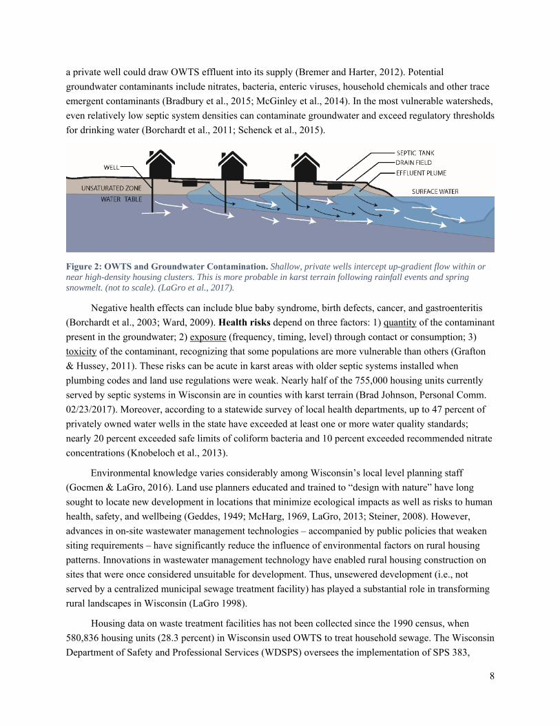
8
a private well could draw OWTS effluent into its supply (Bremer and Harter, 2012). Potential
groundwater contaminants include nitrates, bacteria, enteric viruses, household chemicals and other trace
emergent contaminants (Bradbury et al., 2015; McGinley et al., 2014). In the most vulnerable watersheds,
even relatively low septic system densities can contaminate groundwater and exceed regulatory thresholds
for drinking water (Borchardt et al., 2011; Schenck et al., 2015).
Figure 2: OWTS and Groundwater Contamination. Shallow, private wells intercept up-gradient flow within or near high-density housing clusters. This is more probable in karst terrain following rainfall events and spring snowmelt. (not to scale). (LaGro et al., 2017).
Negative health effects can include blue baby syndrome, birth defects, cancer, and gastroenteritis
(Borchardt et al., 2003; Ward, 2009). Health risks depend on three factors: 1) quantity of the contaminant
present in the groundwater; 2) exposure (frequency, timing, level) through contact or consumption; 3)
toxicity of the contaminant, recognizing that some populations are more vulnerable than others (Grafton
& Hussey, 2011). These risks can be acute in karst areas with older septic systems installed when
plumbing codes and land use regulations were weak. Nearly half of the 755,000 housing units currently
served by septic systems in Wisconsin are in counties with karst terrain (Brad Johnson, Personal Comm.
02/23/2017). Moreover, according to a statewide survey of local health departments, up to 47 percent of
privately owned water wells in the state have exceeded at least one or more water quality standards;
nearly 20 percent exceeded safe limits of coliform bacteria and 10 percent exceeded recommended nitrate
concentrations (Knobeloch et al., 2013).
Environmental knowledge varies considerably among Wisconsin’s local level planning staff
(Gocmen & LaGro, 2016). Land use planners educated and trained to “design with nature” have long
sought to locate new development in locations that minimize ecological impacts as well as risks to human
health, safety, and wellbeing (Geddes, 1949; McHarg, 1969, LaGro, 2013; Steiner, 2008). However,
advances in on-site wastewater management technologies – accompanied by public policies that weaken
siting requirements – have significantly reduce the influence of environmental factors on rural housing
patterns. Innovations in wastewater management technology have enabled rural housing construction on
sites that were once considered unsuitable for development. Thus, unsewered development (i.e., not
served by a centralized municipal sewage treatment facility) has played a substantial role in transforming
rural landscapes in Wisconsin (LaGro 1998).
Housing data on waste treatment facilities has not been collected since the 1990 census, when
580,836 housing units (28.3 percent) in Wisconsin used OWTS to treat household sewage. The Wisconsin
Department of Safety and Professional Services (WDSPS) oversees the implementation of SPS 383,
9
which provides laws and regulations pertaining to the design, installation, and maintenance of OWTS
(WDSPS, 2000). The agency stopped maintaining a comprehensive record of wastewater treatment types
per housing unit (WDSPS, 2000), but recently completed a statewide county-by-county inventory in
2017. We estimate that nearly 755,000 housing units in Wisconsin are currently served by OWTS.
Currently this inventory information is kept by each county making it difficult to obtain real-time
information regarding OWTS for the entire state. WDSPS only maintains records of the inventory status
with system totals for each county (Bradley Johnson, Personal Communication 2/23/2017).
Typically, households with a private OWTS also have a private well. About 800,000 private wells
in Wisconsin provide drinking water where municipal services are not available (Vogt et al., 2017). Siting
standards can vary at the local municipal level. When siting new development, OWTS and well locations
are typically determined by setbacks from parcel boundaries and by distances from a private well. The
location of neighboring systems and private wells, the direction of groundwater flow, and the underlying
hydrogeology are given less, if any, consideration. Maintenance of private wells and OWTS are the
responsibility of individual homeowners, yet effluent from neighboring septic systems can be drawn into
private drinking water supply wells (Bremer and Harter, 2012). Moreover, a lack of well stewardship
among rural homeowners means approximately 10 percent of homeowners test their wells regularly
(Maleki et al, 2017). In locations where OWTS densities exceed the soil’s ability to effectively filter
effluent, private wells may become contaminated without the knowledge of the homeowners (USGS,
ND).
Clustering of homes in peri-urban (or exurban) landscapes served by private wells and private
onsite wastewater treatment systems (OWTS) has potentially significant implications for environmental
quality and public health. Recent studies indicate that rural residential development using OWTS, even in
relatively lower densities, could lead to concentrations of groundwater contaminants above regulated
thresholds (Schenck et al. et al., 2015; Borchardt et al. 2011; Rayne et al. 2011). Many of these systems
are installed in clusters of single-family homes with lot sizes varying from one-half to two or more acres.
These risks are more likely where OWTS were not installed correctly or were installed when regulatory
standards were far less stringent than today, or where OWTS are near the end of their expected life spans
or are not maintained properly. However, systems may be installed properly and still could pose
significant risks in some areas (Borchardt et al., 2003; Borchardt et al., 2011). Adjacent to lakes and along
rivers, for example, unsewered development can have significant implications for environmental quality
and both ecosystem and human health.
Although some research has examined the relationship between unsewered subdivisions and
groundwater quality (McGinley et al. et al., 2015; WGNHS, 2015; Rayne and Bradbury, 2011; Rayne et
al., 2018), that research has focused on areas with newer subdivisions or larger lot sizes than often occur
in peri-urban settings near major metropolitan areas. One study found a correlation between OWTS
density and infectious diseases, especially among children, by aggregating system density and health data
by census blocks (Borchardt et al., 2003). Another study examined the correlation between trace
contaminants in surface water and the surrounding land uses and waste water treatment practices but
acknowledges the presence of point and non-point pollutant sources that confound statistical analysis to
determine the source of such contaminants (Schenck et al., 2015). Studies from other states (North
10
Carolina) and other countries (UK, Australia), have identified densely clustered OWTS as a significant
human health risk. These studies illustrate the value of spatially-explicit analyses and targeted
interventions to protect groundwater quality and manage health risks within these coupled natural-human
systems.
3. Research Design The study area for this research encompasses landscapes draining into the Milwaukee Estuary, a
designated Area of Concern (AOC) by the U.S. EPA and the Wisconsin Department of Natural Resources
(DNR). A geographic information system (GIS) integrated geospatial data on: a) hydrogeology (depth to
aquifer; depth to water table; aquifer and over-burden permeability; groundwater flow direction,
groundwater vulnerability); b) land use patterns and practices (residential septic system type, age, and
density; private well depth, age, and design); and c) land use policies (zoning codes, subdivision
standards, private septic system and water well siting standards). In an earlier study, OWTS parcel data
were used to identify rural residential development clusters within Ozaukee County (LaGro et al., 2017).
Those methods were employed in this study to update parcel and OWTS data. These spatial data layers
were compared, in a GIS overlay analysis, with existing regional groundwater flow models, vulnerability
assessments, and recharge data available from the Wisconsin Geological and Natural History Survey
(WGNHS). OWTS point data were mapped over regional land use data using parcel centroids associated
with active OWTS permits at the Ozaukee County Land and Water Management . A point density surface
map was generated and used to identify areas with highest densities of OWTS (Mitchell, 2005; Lloyd,
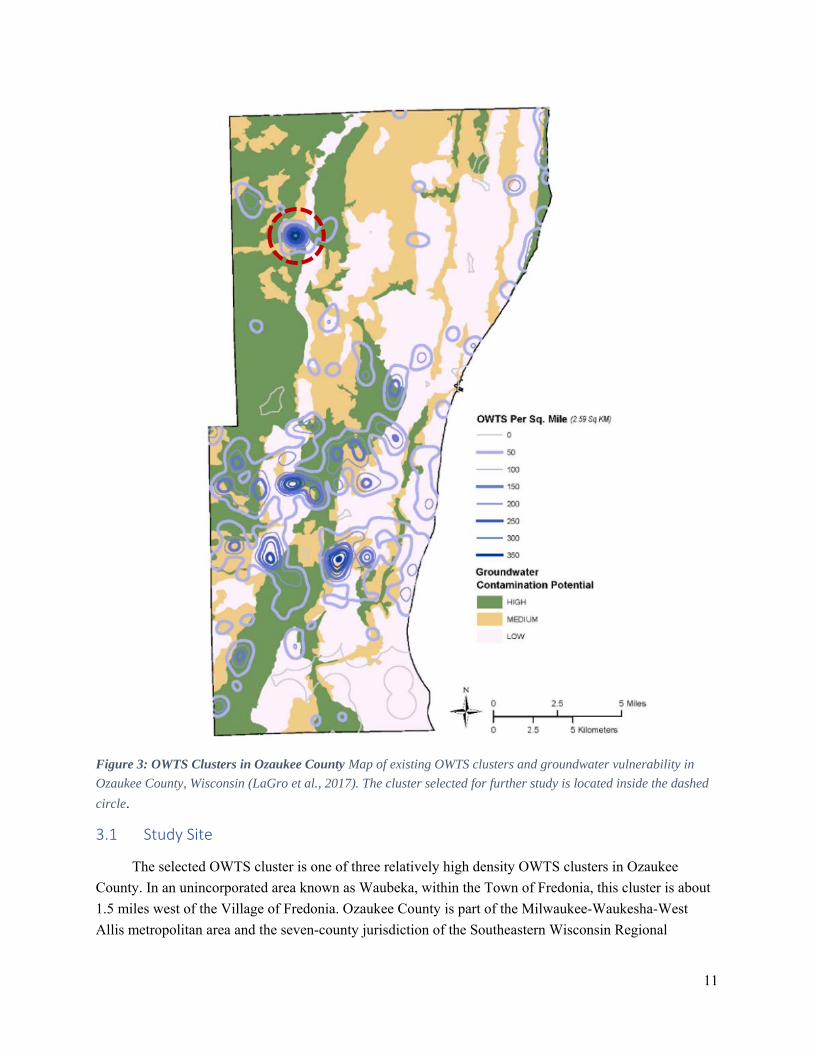
2010). An overlay analysis of GIS data layers identified “hot spots” (i.e., locations with high groundwater
contamination potential and high OWTS densities (Figure 3). This northernmost hot spot was selected for
our pilot study.
11
Figure 3: OWTS Clusters in Ozaukee County Map of existing OWTS clusters and groundwater vulnerability in
Ozaukee County, Wisconsin (LaGro et al., 2017). The cluster selected for further study is located inside the dashed
circle.
3.1 Study Site
The selected OWTS cluster is one of three relatively high density OWTS clusters in Ozaukee
County. In an unincorporated area known as Waubeka, within the Town of Fredonia, this cluster is about
1.5 miles west of the Village of Fredonia. Ozaukee County is part of the Milwaukee-Waukesha-West
Allis metropolitan area and the seven-county jurisdiction of the Southeastern Wisconsin Regional

12
Planning Commission (SEWRPC). Ozaukee County is located just north of the City of Milwaukee along
the western shores of Lake Michigan. Its total land area is 223 square miles (578 km2), with sixteen
municipal civil divisions comprising seven villages, six towns, and three cities. Between 1960 and 2010,
both the population and number of households in the county more than doubled (SEWRPC, 2004). The
county had 86,395 residents and 36,267 housing units in 2010, for an average household size of 2.47
persons (US Census Bureau, 2013). About 22% of the county’s housing units relied upon private on-site
wastewater systems, in contrast with 11% of all households in the 7-county SEWRPC region (M. Hahn,
personal communication, August 11, 2016).
Ozaukee County’s landscape consists of nearly level to rolling farmland with the largest wooded
areas located mostly on steeper topography bordering Lake Michigan and along major drainage corridors.
The parent material for most soils in the county was deposited as glacial till during the most recent
glaciation (10,000 BP). Incomplete drainage of this poorly dissected landscape has led to the formation of
many small scattered marshes and lakes (USDA, 1970). The Milwaukee River flows north to south in the
county, dividing the better-drained loamy soils west of the river from the more poorly-drained silt clay
loam soils near Lake Michigan. In places, the county’s soils are relatively shallow (generally less than 36
in., or 0.914 meters) and are primarily underlain by a fractured dolomite bedrock with cracks and large
pores that enable rapid groundwater movement within this karst terrain (WGNHS, 2013).
3.2 Household Surveys
A mail survey was distributed to home-owners with design guidance from UW-Madison Survey
Center (UWSC), UW Extension Bulk Mailing, and UW-Madison Department of Information Technology
Digital Publishing and Printing Services. A total of 233 surveys were mailed to home-owners in four
township sections, within the Town of Fredonia, encompassing an unincorporated area known as
Waubeka (about 1.5 miles west of the Village of Fredonia). The initial sampling frame for the four
township sections consisted of all properties with an active OWTS permit on record at the county Land
and Water Management office. Businesses and homeowners who did not reside at the permit record
address were subsequently excluded from the sampling frame. We used the UWSC 3-wave mail screener
protocol which includes: 1) Wave 1: letter introducing the study, the 4-page survey, and postage paid
return envelope with a $2 cash incentive; 2) Wave 2: a postcard reminder to return the survey; and Wave
3: Repeat of Wave 1 for those who had not yet responded at the time of that mailing. Each wave was
mailed approximately 2 weeks apart beginning in early April 2017. The water quality portion’s sampling
framework was completed using information obtained during the survey. Surveys were received through
July 2017, but only those received prior to June 1 were considered for water quality sampling. Free
private well water tests were the only incentive offered to prospective participants. To maximize
participation and to minimize homeowner concerns about confidentiality in such a limited/small sample,
we did not request information on household socioeconomic status (e.g., education, income, health, or
political affiliation). IRB approval was maintained throughout the duration of the project to protect
homeowners’ privacy.

13
Figure 4: Waubeka Study Area: a) map of parcels and OWTS systems, by type; b) map of groundwater vulnerability, based on hydrogeological conditions; c) map of OWTS density per acres. Note: study area is bisected by the Milwaukee River. (Adapted from LaGro et al., 2017).
14
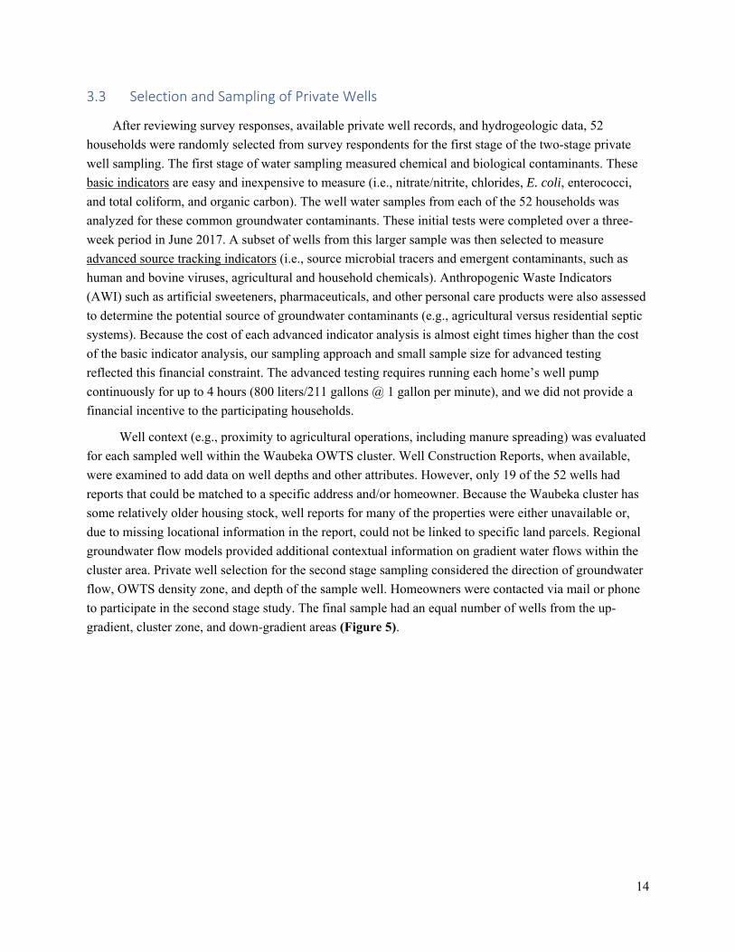
3.3 Selection and Sampling of Private Wells
After reviewing survey responses, available private well records, and hydrogeologic data, 52
households were randomly selected from survey respondents for the first stage of the two-stage private
well sampling. The first stage of water sampling measured chemical and biological contaminants. These
basic indicators are easy and inexpensive to measure (i.e., nitrate/nitrite, chlorides, E. coli, enterococci,
and total coliform, and organic carbon). The well water samples from each of the 52 households was
analyzed for these common groundwater contaminants. These initial tests were completed over a three-
week period in June 2017. A subset of wells from this larger sample was then selected to measure
advanced source tracking indicators (i.e., source microbial tracers and emergent contaminants, such as
human and bovine viruses, agricultural and household chemicals). Anthropogenic Waste Indicators
(AWI) such as artificial sweeteners, pharmaceuticals, and other personal care products were also assessed
to determine the potential source of groundwater contaminants (e.g., agricultural versus residential septic
systems). Because the cost of each advanced indicator analysis is almost eight times higher than the cost
of the basic indicator analysis, our sampling approach and small sample size for advanced testing
reflected this financial constraint. The advanced testing requires running each home’s well pump
continuously for up to 4 hours (800 liters/211 gallons @ 1 gallon per minute), and we did not provide a
financial incentive to the participating households.
Well context (e.g., proximity to agricultural operations, including manure spreading) was evaluated
for each sampled well within the Waubeka OWTS cluster. Well Construction Reports, when available,
were examined to add data on well depths and other attributes. However, only 19 of the 52 wells had
reports that could be matched to a specific address and/or homeowner. Because the Waubeka cluster has
some relatively older housing stock, well reports for many of the properties were either unavailable or,
due to missing locational information in the report, could not be linked to specific land parcels. Regional
groundwater flow models provided additional contextual information on gradient water flows within the
cluster area. Private well selection for the second stage sampling considered the direction of groundwater
flow, OWTS density zone, and depth of the sample well. Homeowners were contacted via mail or phone
to participate in the second stage study. The final sample had an equal number of wells from the up-
gradient, cluster zone, and down-gradient areas (Figure 5).

15
Figure 5: Well Sampling Framework Schematic plan view of a housing cluster (black dots) illustrating the range of housing densities that can exist along groundwater flow paths. Wells were sampled across a variety of densities and well construction periods for the Waubeka study area.
3.3.1 Basic Indicator Analysis
Well samples were drawn on the following dates in 2017: June 12, 20, and 28. Groundwater
analyzed for nitrate and bacteria (total coliform, E. coli, enterococcus) was collected from an outside,
unfiltered/unsoftened water spigot or hydrant in high-density polyethylene (HDPE) bottles, stored at 4ºC,
and delivered to the lab within 40 hours of sample collection. The samples were analyzed with a Lachat
flow injection analyzer for nitrate (Lachat Method 10-107-04-1-A). Coliform, E. coli and enterococcus
testing used US EPA approved enzyme substrate methods with dilution for quantification (IDEXX,
Westbrook, Maine). Groundwater analyzed for nitrate and bacteria (total coliform, E. coli enterococcus)
was collected using standard analyte selection methods and sample preparation and analysis techniques
(McGinley et al. et al., 2015; Nitka, 2014).
3.4 Advanced Indicator Analysis
3.4.1 Chemical Analytes & Sample Preparation/Analysis
Chemical tracing to identify nitrate sources has been explored for decades (Aravena et al., 1993;
Wassenaar, 1995; Vengosh & Pankratov, 1998) through contrasts in inorganic hydrochemistry (e.g.,
chloride, boron) and isotopes (e.g., 15N, 18O). The chemical source tracing in this study is focused on
testing, refining and developing methods for the analysis of mobile and recalcitrant organic compounds
that accompany nitrate during recharge to groundwater. It seeks to employ tracers that can provide a
relatively unambiguous resolution of nitrate sources, and, in addition, provide a characterization that can
be communicated directly to land managers and policy makers. For example, the artificial sweeteners
sucralose and acesulfame are relatively unambiguous tracers that are both recalcitrant to wastewater
treatment (Subedi & Kannan, 2014) and are now ubiquitous in human wastewater as evidenced by their
detection in shallow monitoring wells in suburban areas (Van Stempvoort et al., 2011; McGinley et al.,
2015).

16
The private wells chosen for more advanced analysis were sampled by a trained technician using
dead-end ultra-filtration, a method standardized by the Centers for Disease Control and Prevention for
concentrating pathogens from surface water and groundwater (Smith & Hill, 2009). Each well sample was
collected at a typical rate of 0.5 to 1.2 gallons per minute (2.25 - 5.5 liters per minute) for 3.0 to 4.5 hours.
Advanced chemical source tracking samples were collected in 1 liter amber glass bottles after the dead-
end filtered microbial samples were collected. All groundwater samples analyzed for chemical
metabolites were processed at the University of Wisconsin-Stevens Point Water and Environmental
Analysis Laboratory (WEAL). Groundwater samples were analyzed for the on-site wastewater treatment
system suite of pharmaceuticals, personal care, food products and chloroacetanilide herbicide metabolites.
Standard analyte selection methods and sample preparation and analysis techniques were used to track
nitrate contamination from common agricultural or household sources (McGinley et al. et al., 2015; Nitka,
2014; Schenck et al., 2015). A group of twelve (12) pharmaceuticals and personal care products (PPCPs)
unique to human use were chosen to identify wells likely impacted by OWTS. A bovine antibiotic and six
(6) chloroacetanilide herbicide metabolites (CAAMs) were used to identify contamination from
agricultural sources. The results of these analyses were interpreted using the spatial location of the sample
site in relation to the OWTS cluster, groundwater flow model, well depth, and surrounding land use.
Similar methods have been used to determine the source of potential groundwater contamination where
multiple pollution sources exist near private wells (Nitka, 2014; McGinley et al., 2015).
3.4.2 Microbial Analytes & Sample Preparation/Analysis
A large volume (800 – 1300 L) of well water was sampled from flame-sterilized outdoor taps with
dead-end ultrafiltration (Smith and Hill 2009) using Hemodialyzer Rexeed-25s filters (Asahi Kasei
Medical MT Corp., Oita, Japan). Water was allowed to flow for at least 10 minutes prior to the
spigot/hydrant being attached to the sampling equipment. Field sanitation procedures were implemented
prior to equipment set up and sample collection. Filters were stored on ice and back flushed within 60
hours of sample collection, and polyethylene glycol precipitation was used to further concentrate samples
(Lambertini et al. 2008). Nucleic acids were extracted using QIAamp DNA blood mini kit with a
QIAcube® (Qiagen, Valencia, CA), and virus RNA was reverse transcribed using random hexamers
(ProMega, Madison, WI) and SuperScript® III reverse transcriptase (Invitrogen Life Technologies,
Rockville, MD) following procedures described in Stokdyk et al. (2016). PCR analysis is a test for the
presence of microbial genetic material. It is not a test for live viable microorganisms, but it can be used as
a screening tool for live viable microbes that can then be used to determine their species of origin.
Samples were tested for 1) human-specific microbial genetic material from: adenovirus groups A,
B, C, D, and F, enterovirus, norovirus genogroups I and II, human polyomavirus, hepatitis A virus, and
human-associated HF183 Bacteroides (16S rRNA); 2) bovine-specific microbial genetic material: bovine
polyomavirus, bovine Bacteroides (16S rRNA), and bovine-associated M2 and M3 bacteria; and 3) non-
specific microbial genetic material found in fecal wastes of humans, bovines, and other animals: pepper
mild mottle virus, rotavirus group A (two gene targets), Campylobacter jejuni, Salmonella species (two
gene targets), enterohemorrhagic E. coli (three gene targets), Cryptosporidium species, and Giardia
lamblia (Table). qPCR was performed using a LightCycler® 480 instrument (Roche Diagnostics,
17
Mannheim, Germany) following procedures described in Stokdyk et al. (2016). Hydrolysis probes were
used for quantification, and standard curves were created from gBlocks® and Ultramer® oligos
(Integrated DNA Technologies, Coralville, IA; Table). Following Gibson et al. (2012), lambda phage
DNA and hepatitis G virus armored RNA were used to evaluate all samples for inhibition of qPCR and
reverse transcription-qPCR, respectively. Negative controls were included at all processing steps
(secondary concentration, nucleic acid extraction, reverse transcription, and qPCR) and must exhibit no
fluorescence above the baseline. Modified live virus vaccines (Zoetis Inc., Kalamazoo, MI) were used for
DNA (bovine herpes virus) and RNA (bovine respiratory syncytial virus) extraction positive controls,
with the latter serving also as the reverse transcription positive control.
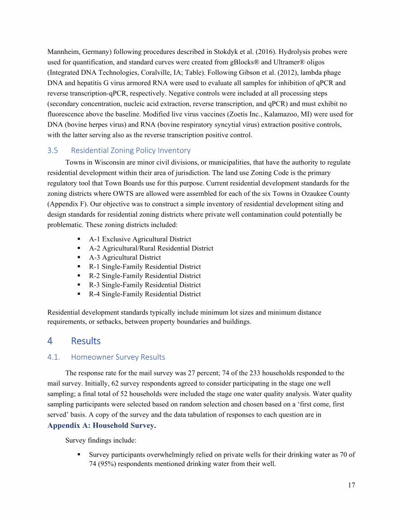
3.5 Residential Zoning Policy Inventory
Towns in Wisconsin are minor civil divisions, or municipalities, that have the authority to regulate
residential development within their area of jurisdiction. The land use Zoning Code is the primary
regulatory tool that Town Boards use for this purpose. Current residential development standards for the
zoning districts where OWTS are allowed were assembled for each of the six Towns in Ozaukee County
(Appendix F). Our objective was to construct a simple inventory of residential development siting and
design standards for residential zoning districts where private well contamination could potentially be
problematic. These zoning districts included:
A-1 Exclusive Agricultural District A-2 Agricultural/Rural Residential District A-3 Agricultural District R-1 Single-Family Residential District R-2 Single-Family Residential District R-3 Single-Family Residential District R-4 Single-Family Residential District
Residential development standards typically include minimum lot sizes and minimum distance requirements, or setbacks, between property boundaries and buildings.
4 Results
4.1. Homeowner Survey Results
The response rate for the mail survey was 27 percent; 74 of the 233 households responded to the
mail survey. Initially, 62 survey respondents agreed to consider participating in the stage one well
sampling; a final total of 52 households were included the stage one water quality analysis. Water quality
sampling participants were selected based on random selection and chosen based on a ‘first come, first
served’ basis. A copy of the survey and the data tabulation of responses to each question are in
Appendix A: Household Survey.
Survey findings include:
Survey participants overwhelmingly relied on private wells for their drinking water as 70 of 74 (95%) respondents mentioned drinking water from their well.
18
Surprisingly, most survey respondents (52 of 74, 78%) mentioned that they were not worried about well contamination issues. Only one respondent mentioned having had an actual contamination problem. About one-half of survey respondents (35 of 74, 47%) had mentioned sampling their well for common contaminants at least once. However, most of the responses indicated that homeowners only sampled after installing a well, purchasing the home, or when water was discolored or had an odor. Meaning that water quality testing was not a regular part of their home maintenance regimen. It is somewhat surprising that most homeowners were confident that their water was safe for drinking, but they had no evidence on which to base that confidence. This indicates that outreach efforts for private well owners/users need to inform/educate on proper sampling schedules, times to sample, and what tests should be completed.
Regarding septic systems, mounds were the most common septic system used (29 out of 71, 41%) followed by conventional systems (21 of 71, 30%), and holding tanks (12 out of 71, 17%).
Most OWTS in our survey were aged 15 to 24 years (23 of 74, 31%). OWTS aged 0 to 14 years and 25 to 44 years made up 17 (23%) and 16 (22%) of our 74 respondents, respectively. 14 (19%) of the 74 OWTS were 45 years or older.
Regarding well depths, most respondents (21 of 70, 30%) did not know the depth of their well. Of those who knew the depth, 29% (20 of 70) reported well depths under 99 feet. 21% (15 of 70) of the households reported wells 150 to 249 feet deep; 16% (11 of 70) reported depths of 100 to 149 feet. Only 3 households (4%) reported well depths greater than 250 feet.
Most respondents (59 of 73, 81%) mentioned spending less than $250 annually on OWTS maintenance. The most common maintenance tasks competed by households were system inspections every 4 years (55 of 68, 82%) and pumping the OWTS out (67 of 73, 92%). Most households had made efforts to reduce kitchen waste, household cleaners, and pharmaceuticals/personal care products going into their OWTS.
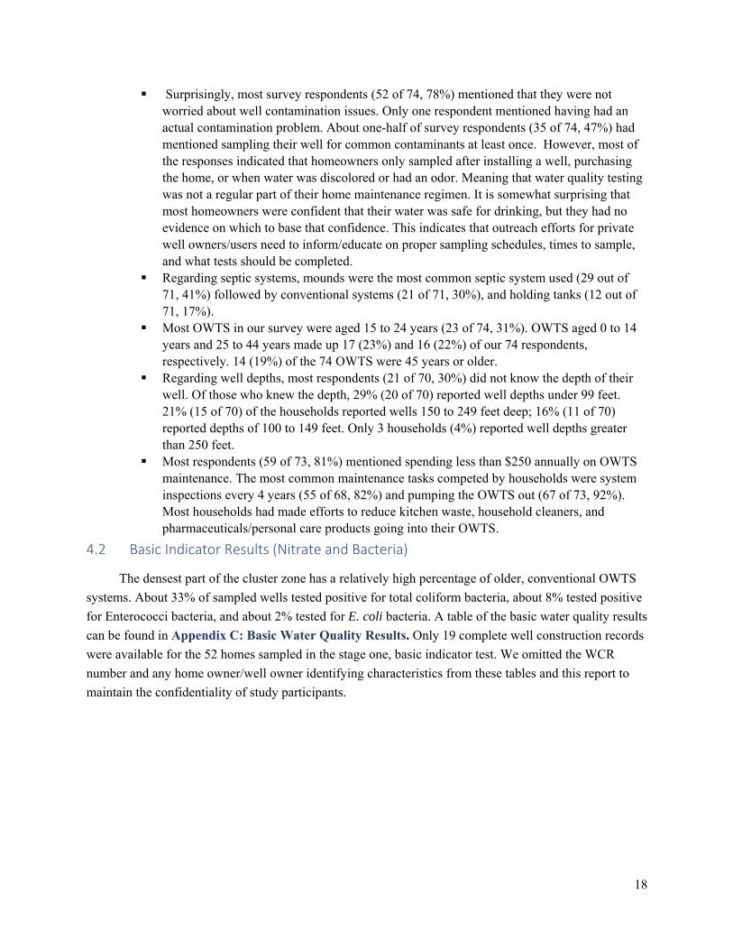
4.2 Basic Indicator Results (Nitrate and Bacteria)
The densest part of the cluster zone has a relatively high percentage of older, conventional OWTS
systems. About 33% of sampled wells tested positive for total coliform bacteria, about 8% tested positive
for Enterococci bacteria, and about 2% tested for E. coli bacteria. A table of the basic water quality results
can be found in Appendix C: Basic Water Quality Results. Only 19 complete well construction records
were available for the 52 homes sampled in the stage one, basic indicator test. We omitted the WCR
number and any home owner/well owner identifying characteristics from these tables and this report to
maintain the confidentiality of study participants.

19
Table 1: Pearson Correlation Coefficients Prob > |r| under H0: Rho=0
Number of Observations
VARIABLE TOTAL
COLIFORM NITRATE
HOME ELEVATION
OWTS DENSITY
HOME AGE
WELL DEPTH
TOTAL COLIFORM
1 ‐0.18518 ‐0.257 0.3178 0.33751 ‐0.2087 0.1888 0.0663 0.0217 0.0154 0.2517
52 52 52 52 51 32
NITRATE ‐0.18518 1 0.319 ‐0.095 ‐0.1421 ‐0.0137
0.1888 0.0212 0.5023 0.3199 0.9405
52 52 52 52 51 32
HOME ELEVATION
‐0.2566 0.31901 1 ‐0.378 ‐0.3048 0.36851
0.0663 0.0212 0.0057 0.0296 0.038
52 52 52 52 51 32
OWTS DENSITY
0.31776 ‐0.09514 ‐0.378 1 0.58515 ‐0.4149
0.0217 0.5023 0.0057 <.0001 0.0182
52 52 52 52 51 32
HOME AGE 0.33751 ‐0.14208 ‐0.305 0.5852 1 ‐0.4815
0.0154 0.3199 0.0296 <.0001 0.0053
51 51 51 51 51 32
WELL DEPTH
‐0.2087 ‐0.01374 0.3685 ‐0.415 ‐0.4815 1
0.2517 0.9405 0.038 0.0182 0.0053
32 32 32 32 32 32
4.3 Advanced Chemical Sourcing Results
Only five of the 14 samples (35.7%) contained artificial sweeteners. No other chemicals were found
in the samples. A table of the advanced chemical sourcing results can be found in Appendix D:
Advanced Chemical Sourcing Results.
4.4 Advanced Microbial Sourcing Results
No source microbial source tracking microbes were detected using the qPCR dead-end filtration
method. A table of the advanced microbial sourcing results can be found in Appendix E: Advanced
Microbial Sourcing Results.
4.5 Residential Zoning Policy Inventory
A summary table of the residential development standards in Ozaukee County’s six Towns can be found
in Appendix F: Residential Zoning Policy Inventory. The cluster study area, in unincorporated
Waubeka, has its own R-4 zoning district (standards are shown below). Notably, the zoning code text
(excerpted below) includes a reference to expected public sanitary sewerage service; as of the date of this
report, those services are not currently available to the households in this cluster.
R-4 SINGLE-FAMILY RESIDENTIAL DISTRICT
“The R-4 District is intended to provide for single-family residential development at densities not to
exceed 6.05 dwelling units per net acre, served by public sanitary sewerage facilities. This district is

20
intended to accommodate existing development in the unincorporated area of Waubeka and shall not
be applied to areas outside of Waubeka.”
The minimum required lot area in the R-4 zoning district is 7,200 square feet. Although lots of this size
currently exist in Waubeka, when clustered together, these lots are far too small to safely accommodate
private wells and private on-site septic systems.
Since 2000, local land use policies have changed to reflect ongoing concerns about unsewered
housing density. Changes to policies mean more restrictions have been placed on subdivision
development in particular larger minimum lot sizes and setback requirements. However, areas with high
densities of OWTS precede most meaningful local land use policies to protect drinking water quality.
This means that in Waubeka and other areas like it, these older development patterns and practices were
‘grandfathered’ in (e.g., zoning variances issued to allow conditions that do not conform with current land
use regulations). Extending water and sewer services to these non-conforming areas is a policy option, but
one with significant financial implications. According to one or more homeowners in this study, a plan
has been developed to extend water and sewer to Waubeka at a cost of $20,000 to $30,000 per
homeowner. But this was not confirmed with the town or village board. SEWRPC has confirmed,
however, that areas like Waubeka are in Sewer Service Expansion areas. Yet, SEWRPC has no authority
or funding sources to make those decisions and can only advise villages and townships that are
considering this option.
5 Discussion This research focused on groundwater quality and related site-specific conditions for a relatively
small area within Ozaukee County’s exurban landscape. This study area was selected after conducting an
analysis of the spatial distribution of OWTS within Ozaukee County. This analysis identified three
relatively dense clusters of residential parcels served by private septic systems. These clusters occur in
areas with carbonate bedrock and varying depths to bedrock, creating hydrogeologic conditions that vary
in their perceived vulnerability to groundwater contamination. The Waubeka study area is unincorporated
and its land use patterns reflect several decades of incremental residential development and land use
change. While the surrounding area has been farmed for decades, residential development unrelated to
local farming has been a more recent (post World War II) phenomenon. The current land use pattern
reflects a relatively slow process of incremental subdivision of larger lots into two or more parcels, with
subsequent residential development on the smaller parcels. The resulting land use mosaic is a
combination of older and relatively small residential parcels (e.g., less than one acre) and newer,
somewhat larger (e.g., two acres or more) residential parcels, surrounded by cropland. Each of these
residential parcels is served by a private water well and a septic system of one of three general types:
conventional, alternative, or holding tank (LaGro, 1996). The Milwaukee River bisects this gently hilly
(e.g., slopes less than 15 percent) study area. Nutrients – in the form of cow manure – are typically spread
on nearby cropland in the spring. Manure spreading was taking place during our sampling procedure in
June. On at least one day during each field sampling session, manure was being applied directly across
the road or in the general vicinity of some of the homes sampled. Several homeowners mentioned nearby
dairy farms that trucked their waste to these areas for disposal.

21
Planning and Policy Implications. A complex mix of state and local policy and institutional
factors influence the patterns of exurban housing development in Wisconsin. Comprehensive plans,
zoning codes, subdivision ordinances, and siting standards for septic systems and private wells are local
land use policies that can – if adopted by town or county governments – influence the location, density,
and design of exurban housing development (Juergensmeyer & Roberts, 2013). Subdivision ordinances,
for example, can shape exurban housing patterns by regulating the location, density, sizes, and
configurations of new parcels, as well as infrastructure improvements needed to make property suitable
for development. Land division standards are associated with the land platting process. State enabling
statutes in the U.S. put limits on the local regulation of “parcelization” by exempting from review any
subdivision that is less than five parcels (Prytherch, 2017). In Ohio, each of these exempt subdivision
parcels must be at least five acres in area (Prytherch, 2017), whereas in Wisconsin these parcels must be
1½ acres or smaller (Wis. Stat. §236.02(12). Incremental parcelization (i.e., not triggering subdivision
review) has led to significant landscape changes in Wisconsin, resulting in the fragmentation and
conversion of forest and farmland to residential uses (Haines et al., 2011; Hammer et al., 2004).
Environmental Quality Implications. Many states within the Great Lakes region now have
OWTS performance codes (Macrellis & Douglas, 2009). Yet, these “plumbing” codes are limited to new
OWTS installations and do not address the growing problem of older septic systems that were installed on
relatively smaller parcels before any meaningful policies were implemented (Jaskula & Hohn, 2002).
With a population of approximately 34 million people living in the Great Lakes Basin region, there are
potentially more than 3 million OWTS that could impact groundwater quality and the transport of
contaminants into streams, rivers, and the Great Lakes (Michigan Sea Grant Institute, 2016). In the most
vulnerable landscapes, even relatively low septic system densities can contaminate groundwater and
exceed regulatory thresholds (Borchardt et al., 2011; Rayne & Bradbury, 2011; Schenck et al., 2015).
Contamination risks are most acute for systems that were not installed correctly, are near the end of their
expected life spans, are not properly maintained, or were installed when plumbing codes and
environmental protection regulations were weak.
Wisconsin’s landscape diversity reflects the convergence of three major biomes (northern boreal forest,
eastern deciduous forest, and western prairie) in combination with a rich glacial history (EPA, 2012). Six
Level III Ecoregions lie within the state, and each ecoregion contains a blend of small streams, medium
and large river systems, lakes, wetlands, and other aquatic ecosystem types (Omernik, 1987). The
Southeastern Wisconsin Till Plains’ gentle topography and fertile soils have a high concentration of
cropland interspersed with remnant patches of grassland and forest. This region also contains the state’s
most populous cities, including Milwaukee and Madison. Aquatic ecosystems within this ecoregion have
been substantially impacted by human activity, including the degradation of water quality in several large
rivers and their tributaries (e.g., Rock River and Milwaukee River). Elevated nitrate levels, high bacterial
counts, or other water pollutants frequently result in temporary beach closures within the Great Lake
regions (Corsi et al., 2014; Lenaker et al., 2017; Schoen & Ashbolt, 2010). What is uncertain, however, is
how much of this contamination is attributable to agricultural practices and how much is attributable to
septic systems and other components of the built environment. Advances in water monitoring techniques

22
now enable tracking of groundwater contaminants to their agricultural and/or residential sources
(Borchardt et al., 2011; Bradbury et al., 2013; McGinley et al., 2015; Schenck et al., 2015).
A conceptual framework for future research is a coupled natural-human systems model that
identifies key drivers of both the natural (hydrogeologic) system and the human (exurban housing) system
(Figure 6). Groundwater is a renewable but “open access” natural resource (Bromley & Cernea, 1989),
and public stewardship in the United States is a key component of the public trust doctrine (Saxer, 2010).
Anthropogenic disturbances to hydrogeologic systems may include: 1) surface disturbances (land cover
changes; dispersal of nutrients, chemicals, and pathogens in runoff from farming operations and the built
environment; 2) subsurface disturbances (septic systems releasing effluent into groundwater; private wells
pumping groundwater for human activities). Consequently, land use practices in one part of a landscape
can have substantial impacts on the quality of groundwater pumped by neighboring properties, or even by
properties in more distant communities.
Figure 6: Coupled Natural-Human Systems. Conceptual framework of the coupled natural-human systems framework.
5.1 Lessons Learned
This pilot study contributes to an emerging area of environmental and public health research. This study
integrated existing spatial information (e.g., depth to bedrock maps, groundwater vulnerability maps,
OWTS permit data) to identify specific residential areas with elevated potential risks of groundwater
contamination from clustered septic systems and nearby farming operations. A few lessons, summarized
below, have learned from reviewing the scientific literature and conducting this pilot study.

23
“Hot Spot” Mapping. The evaluation of potential groundwater impacts associated with unsewered
residential development begins by mapping areas where there is both: a) vulnerable hydrogeologic
conditions (e.g., shallow carbonate bedrock) and b) spatially dense clusters of residences served by
private septic systems and private water wells. OWTS density maps are essential tools in assessing
potential household exposure to contaminated groundwater. This first-order landscape-scale analysis
identifies potential OWTS “hot spots” that warrant further investigation and, potentially, targeted
mitigation (e.g., septic system replacement, well water filtering, installation of deeper, community wells).
Spatial and Temporal Variability of Risk. Hydrogeologic systems interact with social and built
environments to influence the dynamics of groundwater flow and contaminant transport over multiple
spatial and temporal scales. Aquifer depth and groundwater flow are affected, for example, by topography
and underlying geological conditions. Groundwater vulnerability varies spatially, therefore, with the
variation in these hydrogeological conditions (e.g., depth to aquifer, depth to water table, aquifer and
overburden permeability). Consequently, households living in lower lying or “down-gradient” locations
may experience comparatively higher risks of well contamination (Figure 5). In coordination with elected
town officials, residents of at-risk housing units could be advised to periodically test their wells for
contaminants. The timing of well sampling also can matter greatly in landscapes, like the Waubeka study
area, that have shallow wells and relatively permeable soils, carbonate bedrock, and shallow bedrock
overburden. Weather conditions – and subsequent groundwater recharge events – are key factors in the
movement of groundwater contaminants.
5.2 Limitations and Future Research
Private Well Records. The state database of private well records is incomplete and, in some cases,
of questionable quality. In our research, it was difficult to acquire well construction information for the
sampled housing units. Consequently, in some cases, we could not determine the well’s depth, design, or
geologic context. Homeowners knew less about wells and septic than expected, yet many home owners
expressed little concern for water quality and had not previously had their wells tested.
Budget Constraints. Sampling for basic indicators was used as a screening tool to build the
sampling frame for advanced tracking analysis. Yet, budget constraints limited the number of wells that
were tested (at a single point in time) for advanced indicators. Follow-up studies could address this
limitation by initiating several tests within a calendar year and within relatively shorter timeframes,
during recharge events (i.e. heavy rainfall, snow melt, etc.) and during drier conditions. This modification
would address the important influence of intra-annual variability in antecedent soil moisture conditions
due to fluctuations in weather events and groundwater recharge. Other research suggests that contaminant
movement is associated with recharge events such as winter thaw and spring/fall rains (Bonness &
Masarik, 2014; Braatz, 2004). The number of advanced samples is not enough for robust statistical
analysis. Also, the delayed timing of the samples in relation to the initial basic sampling and aquifer
recharge meant that we had no results on the advanced analysis to determine the contamination sources.
Future Research. Additional studies could be designed to understand how septic system density
(e.g., 0.5, 1.0, 1.5, or 2.0 or more dwelling units (DU)/acre with OWTS) interacts with hydrogeologic
setting to influence groundwater contamination flow paths under varied weather conditions (Figure 7).
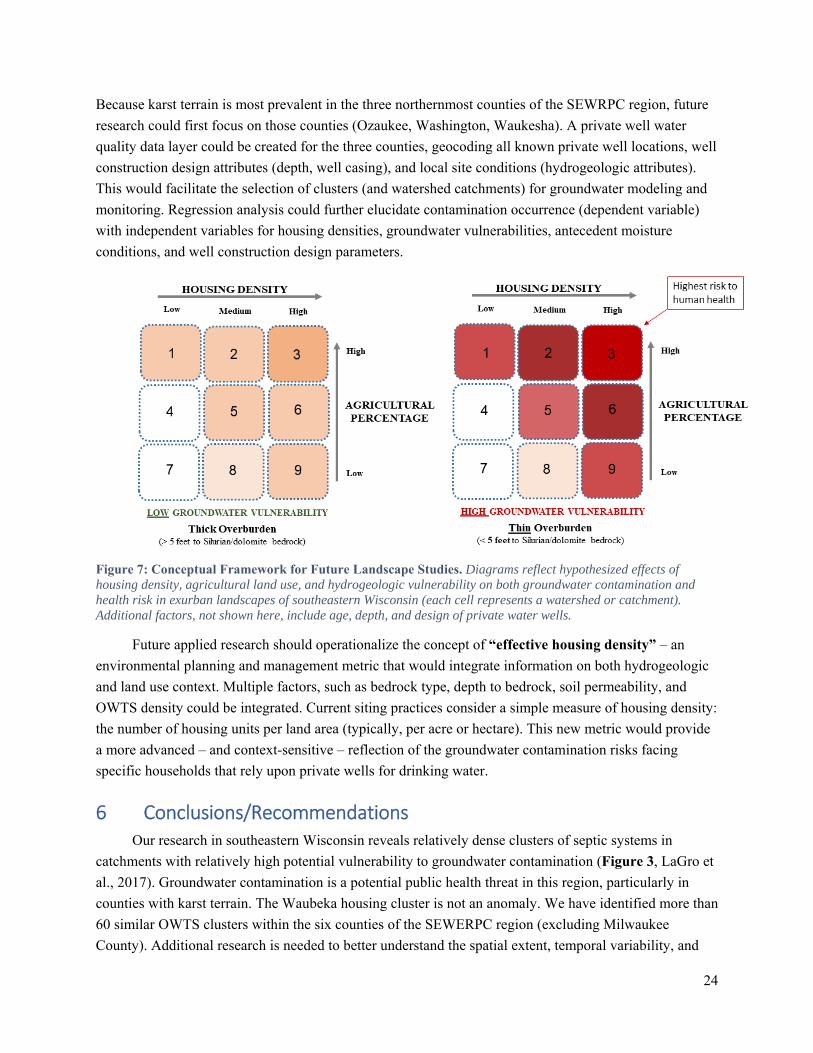
24
Because karst terrain is most prevalent in the three northernmost counties of the SEWRPC region, future
research could first focus on those counties (Ozaukee, Washington, Waukesha). A private well water
quality data layer could be created for the three counties, geocoding all known private well locations, well
construction design attributes (depth, well casing), and local site conditions (hydrogeologic attributes).
This would facilitate the selection of clusters (and watershed catchments) for groundwater modeling and
monitoring. Regression analysis could further elucidate contamination occurrence (dependent variable)
with independent variables for housing densities, groundwater vulnerabilities, antecedent moisture
conditions, and well construction design parameters.
Figure 7: Conceptual Framework for Future Landscape Studies. Diagrams reflect hypothesized effects of housing density, agricultural land use, and hydrogeologic vulnerability on both groundwater contamination and health risk in exurban landscapes of southeastern Wisconsin (each cell represents a watershed or catchment). Additional factors, not shown here, include age, depth, and design of private water wells.
Future applied research should operationalize the concept of “effective housing density” – an
environmental planning and management metric that would integrate information on both hydrogeologic
and land use context. Multiple factors, such as bedrock type, depth to bedrock, soil permeability, and
OWTS density could be integrated. Current siting practices consider a simple measure of housing density:
the number of housing units per land area (typically, per acre or hectare). This new metric would provide
a more advanced – and context-sensitive – reflection of the groundwater contamination risks facing
specific households that rely upon private wells for drinking water.
6 Conclusions/Recommendations Our research in southeastern Wisconsin reveals relatively dense clusters of septic systems in
catchments with relatively high potential vulnerability to groundwater contamination (Figure 3, LaGro et
al., 2017). Groundwater contamination is a potential public health threat in this region, particularly in
counties with karst terrain. The Waubeka housing cluster is not an anomaly. We have identified more than
60 similar OWTS clusters within the six counties of the SEWERPC region (excluding Milwaukee
County). Additional research is needed to better understand the spatial extent, temporal variability, and

25
magnitude of groundwater contamination in this and other Wisconsin regions. These phenomena are not
widely understood at regional, county, or town scales.
Land Use Planning. As the science of coupled natural-human systems improves, new knowledge
can inform better land use decision-making for groundwater protection. For example, geographic
information systems enable the identification of OWTS clusters and – in combination with digital maps of
hydrogeologic conditions – enable estimates of contamination risks at the individual parcel scale of
analysis. Identifying OWTS “hot spots” through cluster analysis is a key step in assessing the scope of the
environmental and public health challenge. Spatially explicit assessments of groundwater contamination
risk can support context-sensitive land use policy and planning and helping to target mitigative
interventions. For example, OWTS siting policies could better reflect the risks associated with some site
contexts.
The spatial analysis tools used in this research could be applied in other landscapes to assess
carrying capacity – the landscape’s intrinsic ability to sustainably provide ecosystem services and
minimize human exposure to environmental health hazards (Steiner, 2008; de Groot et al., 2010). In karst
areas (carbonate bedrock with shallow overburden and high potential groundwater vulnerability), local
land use policies could be adapted to minimize future groundwater contamination risks. These context-
specific adjustments include: a) density restrictions on unsewered housing (implemented through
minimum lot size requirements, for example); b) requirements for deeper private wells and/or deeper
shared subdivision wells; and c) stronger private well construction standards (e.g. greater well casing
depths).
Land Use Policy. Relatively high density clusters of unsewered housing development have been
“grandfathered,” through variances, with more restrictive current zoning (i.e., Waubeka’s R-4 district).
Conflicting land uses – intensive agricultural operations and unsewered housing clusters – create potential
public health risks from periodic contamination of both groundwater and surface waters (e.g., via manure
spreading and, in older residential clusters, from failing septic systems). Aging wastewater and drinking-
water infrastructure in older housing developments, built prior to meaningful environmental regulations,
needs attention from policy-makers. One option is to limit future development of land using private wells
and septic system to only soils that can attenuate contaminants to a safe level through increased transport
times in the unsaturated soil zone. Alternatively, for existing wells and households with potentially
contaminated wells in high density areas, municipal services could be extended, but this would require
substantial new investment.
Groundwater contamination is a hidden problem – out of sight, out of mind. Techniques to make
this human-environment problem more “visible” could improve decision makers understanding of these
complex relationships. The spatially-explicit threats that these phenomena pose for aquatic ecosystems
and human health are significant, but poorly understood. Visualization tools (e.g., 3D digital models)
could be used to demonstrate where groundwater contaminant plumes do (or do not) migrate in response
to weather events like spring snow melt or large spring, summer, or fall rain storms. These tools also have
the potential to model and visualize system responses to weather patterns projected in future climate
scenarios (e.g., wetter, warmer conditions in southeastern Wisconsin).

26
Targeted Well-Testing Program. Well-testing programs should include subsidies for low-income
households to test private wells. Outreach programs in high risk areas could teach homeowners proper
well testing and septic system inspection and care. Well testing results could go to a database system for
private risk assessments. Like cancer registries, the state could make groundwater sampling results
available for health agencies, so pollution issues could be better tracked. If pollution is severe and
widespread in clusters, wells could be enrolled in an advanced source tracking program to identify the
pollution source. This type of information can guide local decision making in addressing unsewered
housing and private well pollution.
Statewide OWTS Permit and Well Record Database. The state’s OWTS permit inventory
requirement should be expanded to provide more guidance for townships and municipalities. For instance,
a common formatting and database entry system for all counties would be useful for uniformly collecting
sate-wide information which could be used with the DNR’s existing well-record system. Well inventories
and septic system inspections could use GPS units to document the exact field location of each. This
geographic information system approach would provide a better state-wide risk assessment tool to
identify targeted groundwater monitoring areas.
Environmental Research. Unraveling the complex flows of contaminants through these exurban
landscapes could benefit from interdisciplinary, complex systems research. Specifically, more research is
needed to better understand the linkages between public policies (e.g., state OWTS standards, local land
use regulations), household decisions (e.g., household residential preferences, OWTS maintenance),
weather (e.g., timing of groundwater recharge events), and groundwater contamination (e.g., risks from
clusters of private septic systems, aquifer flow in karst terrain). Future applied research could address
policy-relevant questions, such as: 1) How does groundwater contamination vary spatially and temporally
within different hydrogeological settings in southeastern Wisconsin? 2) At what housing density
thresholds does groundwater contamination become a significant health risk in these different
hydrogeologic settings? 3) How can this knowledge be used to increase local planning and policy making
capacity and to inform state-level discussions on potential policy revisions that would protect
groundwater quality and human health?
27
7 Sources Cited
1. Appelo, C.A.J. & D. Postma. 2010. Geochemistry, Groundwater, and Pollution, 2nd ed. Boca Raton: CRC Press.
2. Aravena, R., Evans, M. L., Cherry, J. A. 1993. Stable Isotopes of Oxygen and Nitrogen in Source Identification of Nitrate from Septic Systems. Ground Water 31:180-186.
3. Baloch, M. A., & Sahar, L. 2014. Development of a Watershed‐Based Geospatial Groundwater Specific Vulnerability Assessment Tool. Groundwater, 52(S1), 137-147.
4. Bear, J. 2007. Hydraulics of Groundwater, 2nd ed. Mineola, NY: Dover Publications.
5. Berube, A., Singer, A., Wilson, J.H., & Frey, W.H. 2006. Finding Exurbia: America's Changing Landscape at the Metropolitan Fringe. Washington, DC: The Brookings Institution.
6. Borchardt M.A., Spencer S.K., Kieke B.A. Jr., Lambertini E., Loge F.J. 2012. Viruses in non-disinfected drinking water from municipal wells and community incidence of acute gastrointestinal illness. Environ Health Persp, 120:1272-1279.
7. Borchardt, M. A., Bradbury, K. R., Alexander Jr, E. C., Kolberg, R. J., Alexander, S. C., Archer, J. R., … Spencer, S. K. 2011. Norovirus outbreak caused by new septic system in a dolomite aquifer. Ground Water, 49(1), 85-97. doi:10.1111/j.1745-6584.2010.00686.x
8. Borchardt, M.A., Chyou, P.H., Devries, E.O., and Belongia, E.A. 2003. Septic System Density and Infectious Diarrhea in a defined population of children. Environmental Health Perspectives, 111(5) May 2003, pp. 742-748
9. Braatz, L.A. (2004). A Study of Fecal Indicators and other Factors Impacting Water Quality in Private Wells in Door County, WI. MS Thesis. University of Wisconsin – Green Bay.
10. Bradbury, K. R., Borchardt, M. A., Gotkowitz, M., Spencer, S. K., Zhu, J., & Hunt, R. J. 2013. Source and transport of human enteric viruses in deep municipal water supply wells. Environmental science & technology, 47(9), 4096-4103. doi:10.1021/es400509b
11. Bradbury, K.R. 2009. Karst and Shallow Carbonate Bedrock in Wisconsin. Wisconsin Geological and Natural History Survey Factsheet 02. Madison: University of Wisconsin-Extension.
12. Bradbury, K.R., Rayne, T.W., & Krause, J.J. 2015. Impacts of a Rural Subdivision on Groundwater: Results of a Decade of Monitoring. Unpublished project completion report prepared by Wisconsin Geological and Natural History Survey, University of Wisconsin-Madison submitted to Wisconsin Department of Natural Resources, 41 p.
13. Bremer, J.E. and Harter, T. 2012. Domestic wells have high probability of pumping septic tank leachate. Hydrologic Earth System Sciences, 16: 2453-2467.
14. Bromley, D.W. & M.M. Cernea. 1989. The Management of Common Property Natural Resources: Some Conceptual and Operational Fallacies. World Bank Discussion Paper 57. Washington, D.C.: The World Bank.
28
15. Brown, D.G., K.M. Johnson, T.R. Loveland & D.M. Theobold. 2005. Rural land-use trends in the coterminous United States, 1950-2000. Ecological Applications, 15(6): 1851-1863.
16. Butler, D. & Payne, J. 1995. Septic tanks: problems and practice. Building and Environment, 30(3), 419-425. doi:10.1016/0360-1323(95)00012-u
17. Cairney, P., K. Oliver & A. Wellstead. 2016. To bridge the divide between evidence and policy: reduce ambiguity as much as uncertainty. Public Administration Review, 76(3): 399-402.
18. Carrion-Flores, C. & Irwin, E. G. 2004. Determinants of residential land-use conversion and sprawl at the rural-urban fringe. American Journal of Agricultural Economics, 86(4), 889-904.
19. de Groot, R.S., Alkemade, R., Braat, L., Hein, L. & Willemen, L. 2010. Challenges in integrating the concept of ecosystem services and values in landscape planning, management and decision making. Ecological Complexity, 7: 260-272.
20. De Leon R, Shieh C, Baric RS, Sobsey MD. 1990. Detection of enteroviruses and hepatitis A virus in environmental samples by gene probes and polymerase chain reaction, p 833-853. In Proceedings of the 1990 Water Quality Technology Conference. American Water Works Association, Denver, CO.
21. Feinstein, D.T., Hart, D.J., Eaton, T.T., Krohelski, J.T., and Bradbury, K.R. (2004). Simulation of regional groundwater flow in southeastern Wisconsin. Wisconsin Geological and Natural History Survey Open File Report 2004-01.
22. Flynn, R. M., & Sinreich, M. (2010). Characterisation of virus transport and attenuation in epikarst using short pulse and prolonged injection multi-tracer testing. Water Research, 44(4), 1138-1149.
23. Ford, D. & P.W. Williams. 2007. Karst Hydrogeology and Geomorphology. Hoboken, NJ: John Wiley & Sons, [rev. ed.].
24. Forman, R.T.T. 2014. Urban Ecology: Science of Cities. Cambridge: Cambridge University Press.
25. Fortin, M. J., & Dale, M. R. 2014. Spatial Analysis: A Guide for Ecologists. Cambridge University Press.
26. Geddes, P. 1949. Cities in evolution. Williams & Norgate.
27. Geels, F. & J. Schot. 2007. Typology of sociotechnical transition pathways. Research Policy, 36: 399-417.
28. Genskow, K. & D. Wood. 2011. Improving voluntary environmental management programs: facilitating learning and adaptation. Environmental Management, 47: 907-916.
29. Gibson KE, Schwab KJ, Spencer SK, Borchardt MA. 2012. Measuring and mitigating inhibition during quantitative real time PCR analysis of viral nucleic acid extracts from large-volume environmental samples. Water Res 46:4281-4291.
30. Gibson, J.M. & K.J. Pieper. 2017. Strategies to improve well-water quality: A North Carolina perspective. Environmental Health Perspectives, 125(7): 076001.
29
31. Göçmen, Z. A. 2006. Land Development Patterns, Environmental Perceptions, and Residential Preferences in Southeast Michigan. Doctoral dissertation, University of Michigan.
32. Göçmen, Z. A. 2009. Relationships between Residential Development and the Environment: Examining Resident Perspectives. Journal of Planning Education and Research, 29 (1): 54-66.
33. Gӧҫmen, A.Z. & LaGro, Jr., J.A. 2016. Assessing local planning capacity to promote environmentally sustainable residential development. Journal of Environmental Planning and Management, 59(8): 1513-1535. doi:10.1080/09640568.2015.1080673.
34. Gotkowitz, M.B., Zeiler, K.K., Dunning, C.P., Thomas, J., and Lin, Y.-F. 2005. Hydrogeology and Simulation of Groundwater Flow in Sauk County, Wisconsin. Wisconsin Geological and Natural History Survey Bulletin 102, 43 p.
35. Grafton, R.Q. & K. Hussey, eds. 2011. Water Resources Planning and Management. New York: Cambridge University Press.
36. Green HC, Haugland RA, Varma M, Millen HT, Borchardt MA, Field KG, Walters WA, Knight R, Sivaganesan M, Kelty CA, Shanks OC. 2014. Improved HF183 quantitative real-time PCR assay for characterization of human fecal pollution in ambient surface water samples. Applied and environmental microbiology 80:3086-94.
37. Gustafson, E. J., Hammer, R. B., Radeloff, V. C., & Potts, R. S. 2005. The relationship between environmental amenities and changing human settlement patterns between 1980 and 2000 in the Midwestern USA. Landscape Ecology, 20(7), 773-789. doi:10.1007/s10980-005-2149-7
38. Hammer, R. B., Stewart, S. I., Winkler, R. L., Radeloff, V. C., & Voss, P. R. 2004. Characterizing dynamic spatial and temporal residential density patterns from 1940–1990 across the North Central United States. Landscape and Urban Planning, 69(2), 183-199.
39. Hanley, P.F., & Hopkins, L.D., 2007. Do Sewer extension plans affect urban development? A Multiagent simulation. Environment and Planning B, 34(1), 6–27. doi:10.1068/b32061
40. Harrison, M., Stanwyck, E., Beckingham, B., Starry, O., Hanlon, B., & Newcomer, J. (2012). Smart growth and the septic tank: wastewater treatment and growth management in the Baltimore region. Land Ue Policy, 29(3), 483-492.
41. Hart, D.J., Schoephoester, P.R., and Bradbury, K.R. 2012. Groundwater recharge in Dane County, Wisconsin: Estimating recharge using a GIS-based water-balance model. Wisconsin Geological and Natural History Survey Bulletin 107, 11 p.
42. Hastie, T. J. and Tibshirani, R. J. 1990. Generalized Additive Models. New York: Chapman & Hall.
43. Heinz, B., S. Birk, R. Liedl, T. Geyer & K.L. Straub. 2009. Water quality deterioration at a karst spring (Gallusquelle, Germany) due to combined sewer overflow: evidence of bacterial and micro-pollutant contamination. Environmental Geology, 57-797-808.
30
44. Hillebrand, O., K. Nodler, T. Geyer & T. Licha. 2014. Investigating the dynamics of two herbicides at a karst spring in Germany: Consequences for sustainable raw water management. Science of the Total Environment, 482-483: 193-200.
45. Hodder, I. 1994. The Interpretation of Documents and Material Culture. Thousand Oaks, CA: Sage. p. 155. ISBN 0761926879.
46. Hoorfar J, Ahrens P, Rådström P. 2000. Automated 5′ nuclease PCR assay for identification of Salmonella enterica. J Clin Microbiol 38:3429-3435.
47. Jaskula, J.M. & W.A. Hohn. 2002. Potential impacts of Comm 83 on rural groundwater. Water Resources Impact, Small Municipalities and Water Supply, 4(2), 10 – 16. Retrieved from - http://www.awra.org/impact/issues/0203impact.pdf
48. Johnson, B.E. & J. Shifferd. 2016. Who lives where: A comprehensive population taxonomy of cities, suburbs, exurbs, and rural areas in the United States. The Geographical Bulletin, 57: 25-40.
49. Johnson, K.M. and Cromartie, J.B. 2006. The Rural Rebound and its Aftermath. pp. 25-49 in W.A. Kandel and D.L. Brown, eds. Population Change and Rural Society. Springer Netherlands. doi:10.1007/1-4020-3902-6_2
50. Juergensmeyer, J.C. & T.E. Roberts. 2013. Land Use Planning and Development Regulation Law, 3rd ed. St. Paul, Minnesota: Thomson Reuters.
51. Knobeloch, L., Christenson, M., & Anderson, H. 2013. Private drinking water quality in rural Wisconsin. Journal of Environmental Health, 75(7), 16.
52. Kraft, G.J., Mechenich, D.J., and Haucke, J. 2012. Information Support for Groundwater Management in the Wisconsin Central Sands, 2009-2011: Center for Watershed Science and Education, College of Natural Resources, University of Wisconsin - Stevens Point / Extension, 103 p.
53. Krannich, Richard S., Luloff, A.E. & Field, D.R. 2011 People, Places and Landscapes: Social Change in High Amenity Rural Areas. Vol. 14. Springer Science & Business Media. doi:10.5860/choice.49-2999
54. Kuo DW, Simmons F, Xagoraraki I. 2009. A new set of PCR assays for the identification of multiple human adenovirus species in environmental samples. J Appl Microbiol 107:1219-1229.
55. LaGro Jr., J. A. 1996. Designing without nature: unsewered residential development in rural Wisconsin. Landscape and Urban Planning, 35(1), 1-9.
56. LaGro Jr., J.A. 1998. Landscape context of rural residential development in southeastern Wisconsin (USA). Landscape Ecology, 13(2), 65-77.
57. LaGro Jr., J.A., Vowels, B., & Vondra, B. 2017. Exurban housing development, onsite wastewater disposal, and groundwater vulnerability within a changing policy context. Landscape & Urban Planning, 167: 60-71.
58. Lambertini E, Spencer SK, Bertz PD, Loge FJ, Kieke BA, Borchardt MA. 2008. Concentration of enteroviruses, adenoviruses, and noroviruses from drinking water by use of glass wool filters. Appl Environ Microbiol 74:2990-2996.
31
59. Lichter, D.T. & D.L. Brown, 2011. Rural America in an urban society: Changing Spatial and Social Boundaries. Annual Review of Sociology, 37: 565-592.
60. Lichter, D.T. & J. Ziliak. 2017. The rural-urban interface: new patterns of spatial interdependence and inequality in America. Annals of the American Academy of Political and Social Science, 672: 6-25.
61. Lloyd, C. 2010. Spatial data analysis: an introduction for GIS users. Oxford University Press.
62. Macrellis, A. & Douglas, B. 2009. Update of the Advanced On-Site Wastewater Treatment and Management Market Study: State Reports. (05-DEC-3SGc) Water Environment Research Foundation, Alexandria, VA.
63. Malecki, K. M., Schultz, A. A., Severtson, D. J., Anderson, H. A., & VanDerslice, J. A. (2017). Private-well stewardship among a general population based sample of private well-owners. Science of the Total Environment, 601, 1533-1543.
64. Marra, G. and S.N. Wood (2011) Practical variable selection for generalized additive models. Computational Statistics and Data Analysis, 55: 2372-2387.
65. Bonness, D., & Masarik, K. (2014). Investigating intra-annual variability of well water in Lincoln Township. Final Report to Town of Lincoln, WI. Accessed at: http://www.cleanwisconsin.org/wp-content/uploads/2015/01/Ex1_Lincoln_FinalReport.pdf
66. McGinley, P.M., Devita, W.M., & Nitka, A.L. 2015. Evaluating Chemical Tracers in Suburban Groundwater as Indicators of Nitrate-Nitrogen Sources. Prepared by Center for Watershed Science and Education, University of Wisconsin-Stevens Point for the Wisconsin Department of Natural Resources.
67. McHarg, I. 1969. Design With Nature. Garden City, NJ: The Natural History Press.
68. Michigan Sea Grant Institute. 2016. About the Great Lakes. Webpage.
69. Mitchell, A. 2005. The ESRI guide to GIS analysis, Volume 2: Spatial Measurements and Statistics. Redlands, CA: ESRI.
70. Monpoeho S, Dehee A, Mignotte B, Schwartzbrod L, Marechal V, Nicolas JC, Billaudel S, Ferre V. 2000. Quantification of enterovirus RNA in sludge samples using single tube real-time RT-PCR. Biotechniques 29:88-93.
71. Nitka, A.L. 2014. Developing and testing a method for the analysis of chemical human waste markers in groundwater and identifying sources of nitrate contamination (Masters Thesis, University of Wisconsin Stevens Point).
72. Nygren, N.V., A. Jokinen, & A. Nikula. 2017. Unlearning in managing wicked biodiversity problems. Landscape and Urban Planning, 167: 473-482.
73. Osgood Jr, J.L. 2011. Exurban dynamics: an analysis of migration and urban containment policies. Urbana: Urban Affairs and Public Policy, 11, 1 – 27.
74. Ostrum, E. 1990. Governing the Commons: The Evolution of Institutions for Collective Action. Cambridge: Cambridge University Press.

32
75. Parsen, M.J., Bradbury, K.R., Hunt, R.J., and Feinstein, D.T. 2016. The 2016 Groundwater Flow Model for Dane County, Wisconsin. Wisconsin Geological and Natural History Survey Bulletin 110, 56 p.
76. Peiser, R. 2001. Decomposing urban sprawl. The Town Planning Review, 72(3): 275-298.
77. Prytherch, D.L. 2017. Where a subdivision is not a “subdivision”: State enabling statutes and the local regulation (or not) of land division in the United States. Journal of Planning Education and Research, 37(3): 286-298.
78. Radeloff, V.C., Hammer, R.B. & Stewart, S.I. 2005. Rural and suburban sprawl in the U.S. Midwest from 1940 to 2000 and its relation to forest fragmentation. Conservation Biology, 19(3), 793-805. doi:10.1111/j.1523-1739.2005.00387.x
79. Radeloff, V.C., Hammer, R.B., Stewart, S.I., Fried, J.S., Holcomb, S.S., & McKeefry, J.F. 2005. The wildland–urban interface in the United States. Ecological applications, 15(3), 799-805.
80. Rayne, T.W., & Bradbury, K.R. 2011. Evaluating impacts of subdivision density on shallow groundwater in southeastern Wisconsin, USA. Journal of Environmental Planning and Management, 54(5), 559-575.
81. Rayne, T.W., Bradbury, K.R., & Krause, J.J. 2018. Impacts of a rural subdivision on groundwater quality: results of long-term monitoring. Groundwater, doi: 10.1111/gwat.12666
82. Rogers, E. 1995. Diffusion of Innovations, 4th ed. New York: The Free Press.
83. Rome, A. 2001. The Bulldozer in the Countryside: Suburban Sprawl and the Rise of American Environmentalism. Cambridge University Press.
84. Ruppert, D., Wand, M.P., and Carroll, R.J. 2003. Semiparametric Regression, Cambridge: Cambridge University Press.
85. Saxer, S.R. 2010. The fluid nature of property rights in water. Duke Environmental Law & Policy Forum, 21(49): 49-112.
86. Schenck, K., Rosenblum, L., Ramakrishnan, B., Carson, J., Macke, D., & Nietch, C. 2015. Correlation of trace contaminants to wastewater management practices in small watersheds. Environmental Science: Processes & Impacts, 17(5), 956-964.
87. Schoen, M.E. & Ashbolt, N.J. 2010. Assessing pathogen risk to swimmers at non-sewage impacted recreational beaches. Environmental Science & Technology, 44(7), 2286–2291. doi: 10.1021/es903523q
88. Shaw, B.H., Arntsen, P., & VanRyswyk, W. 1993. Subdivision Impacts on Groundwater Quality. Wisconsin Groundwater Management Practice Monitoring Project, [DNR-067]. Wisconsin Department of Natural Resources.
89. Smith CM, Hill VR. 2009. Dead-end hollow-fiber ultrafiltration for recovery of diverse microbes from water. Appl Environ Microbiol, 75:5284-5289.
90. Southeastern Wisconsin Regional Planning Commission (SEWRPC) and Wisconsin Geologic and Natural History Survey (WGNHS). 2002. Groundwater Resources of Southeastern Wisconsin. Technical Report 37. Waukesha and Madison.

33
91. Steiner, F. 2008. The Living Landscape: An Ecological Approach to Landscape Planning, 2nd ed. Washington, D.C.: Island Press.
92. Stillo, F. & J.M. Gibson. 2017. Exposure to contaminated drinking water and health disparities in North Carolina. American Journal of Public Health, 107(1): 180-185.
93. Stokdyk, J.P., Firnstahl, A.D., Spencer, S.K., Burch, T.R. and Borchardt, M.A., 2016. Determining the 95% limit of detection for waterborne pathogen analyses from primary concentration to qPCR. Water research, 96, pp.105-113.
94. Subedi, B. and K. Kannan. 2014. Fate of artificial sweeteners in wastewater treatment plants in New York State, U.S.A. Environ. Sci. Technol. 48:13668-13674.
95. U.S. Census Bureau. 1993. Historical census of housing tables: sewage disposal.
96. U.S. Environmental Protection Agency (USEPA). 2002. Onsite wastewater treatment systems manual. Prepared by the Office of Water, Office of Research and Development.
97. U.S. Environmental Protection Agency (USEPA). 2005. A Homeowner’s Guide to Septic Systems. Prepared by the Office of Water, Office of Research and Development.
98. U.S. Environmental Protection Agency (USEPA). 2012. Identifying and Protecting Healthy Watersheds: Concepts, Assessments, and Management Approaches. U.S. EPA Office of Water.
99. U.S. Environmental Protection Agency (USEPA). 2013. Decentralized Wastewater Management Program Highlights. Annual Report 2013. Decentralized Wastewater Program.
100. United States Geological Survey (USGS) (No Date) Groundwater and the rural homeowner. Report prepared by Waller, R.M., retrieved from http://pubs.usgs.gov/gip/gw_ruralhomeowner/ on 10/14/2015.
101. Van Stempvoort, D. R., Robertson, W. D., & Brown, S. J. 2011a. Artificial sweeteners in a large septic plume. Groundwater Monitoring & Remediation, 31(4), 95-102.
102. Van Stempvoort, D.R., J.W. Roy, S.J. Brown, & G. Bickerton. 2011b. Artificial sweeteners as potential tracers in groundwater in urban environments. J. Hydrology 401:126-133.
103. Vengosh, A. and I. Pankratov, I., 1998. Chloride/bromide and chloride/fluoride ratios of domestic sewage effluents and associated contaminated ground water. Ground Water 36: 815–824.
104. Vesper, D.M., C.M. Loop & W.B. White. 2001. Contaminant transport in karst aquifers. Theoretical and Applied Karstology, 13-14: 101-111.
105. Vogt, C., Irving, R., Camponeschi, J., Christenson, M., & Creswell, P. 2017. What’s in your water? A look at private well water quality in Wisconsin. Surveillance Brief: Wisconsin Environmental Public Health Tracking Program, July 2017.
106. Ward, M.H. 2009. Too much of a good thing? Nitrate from nitrogen fertilizers and cancer. Reviews on Environmental Health, 24(4): 357-363. doi:10.1515/reveh.2009.24.4.357
107. Wassenaar, L. 1995. Evaluation of the origin and fate of nitrate in the Abbotsford aquifer using the isotopes of 15N and 18O in NO3−. Appl. Geochem. 10: 391–405.

34
108. Weary, D. J. & Doctor, D. H. 2014. Karst in the United States: A Digital Map Compilation and Database. Report prepared for the United States Geological Survey.
109. Wheeler, S.M. 2008. The evolution of built landscapes in metropolitan regions. Journal of Planning Education and Research, 27, 400-416.
110. Wheeler, S.M. 2015. Built landscapes of metropolitan regions: an international typology, Journal of the American Planning Association, 81:3, 167-190.
111. Wilcox, J.D., Bradbury, K.R., Thomas, C.L., & Bahr, J.M. 2005. Assessing background ground water chemistry beneath a new unsewered subdivision. Ground Water, 43(6), 787-795. doi:10.1080/01944361003742403
112. Wilcox, J.D., Gotkowitz, M.B., Bradbury, K.R., and Bahr, J.M. 2010. Using groundwater models to evaluate strategies for drinking-water protection in rural subdivisions. Journal of the American Planning Association, 76(3), pp 295- 304.
113. Wisconsin Department of Commerce, Safety and Buildings. (WDOC). 1999. Corry’s POWTS
114. Wisconsin Department of Natural Resources (WDNR) (2015) Wells. Retrieved from http://dnr.wi.gov/topic/wells/ on 10/26/15.
115. Wisconsin Department of Natural Resources (WDNR). 2014. Wisconsin Administrative Code, 2015. Chapter NR 140, Groundwater Quality.
116. Wisconsin Department of Natural Resources (WDNR). 2015. Wells.
117. Wisconsin Department of Safety and Professional Services (WDSPS) (2000) Wisconsin Administrative Code, 2000. Chapter COMM. 83, Private onsite wastewater treatment.
118. Wisconsin Geological and Natural History Survey (WGNHS), 2009. Karst and Shallow Carbonate Bedrock in Wisconsin. UW Extension Fact Sheet 02.
119. Wisconsin Geological and Natural History Survey (WGNHS). (2002) Groundwater resources of southeastern Wisconsin. (Technical Report No. 37) Madison, WI: Prepared for the Southeastern Wisconsin Regional Planning Commission. Retrieved from http://www.sewrpc.org/SEWRPCFiles/Publications/TechRep/tr-037_groundwater_resources.pdf
120. Wisconsin Geological and Natural History Survey (WGNHS). (2008) Groundwater recharge in southeastern Wisconsin estimated by a GIS-based water-balance model (Technical Report No. 47) Madison, WI: Hart, D.J., Schoenphoester, P.R., and Bradbury, K.R. Prepared for the Southeastern Wisconsin Regional Planning Commission. Retrieved from http://www.sewrpc.org/SEWRPCFiles/Publications/TechRep/tr-047_groundwater_recharge.pdf
121. Wisconsin Geological and Natural History Survey (WGNHS). (2013) Wisconsin Aquifers. Retrieved from http://wgnhs.uwex.edu/water-environment/wisconsin-aquifers/ on 10/23/2015.
122. Wisconsin Geological and Natural History Survey (WGNHS). 2015. Impacts of a rural residential subdivision on groundwater: results of a decade of monitoring. Prepared by
35
Bradbury, K.R., Rayne, T. W., and Krause, J.J. for the Wisconsin Department of Natural Resources.
123. Wisconsin State Legislature (WSL). 2008. Public hearing – committee records: Committee on commerce, utility, and rail.
124. Withers, P.J.A., P. Jordan, L. May, H.P. Jarvie & N.E. Deal. 2014. Do septic tank systems pose a hidden threat to water quality? Frontiers in Ecology and the Environment, 12(2): 123-130.
125. Wood S.N. 2017. Generalized Additive Models: An Introduction with R, 2nd ed. Chapman and Hall/CRC Press.
126. Wood, S.N. 2003. Thin plate regression splines. Journal of the Royal Statistical Society: B, 65(1):95-114.
127. Wood, S.N. 2004. Stable and efficient multiple smoothing parameter estimation for generalized additive models. Journal of the American Statistical Association, 99:673-686
128. Wood, S.N. 2006. Low rank scale invariant tensor product smooths for generalized additive mixed models. Biometrics, 62(4):1025-1036
129. Wood, S.N., N. Pya and B. Saefken. 2016. Smoothing parameter and model selection for general smooth models (with discussion). Journal of the American Statistical Association, 111, 1548-1575
130. Yates, M.V. 1985. Septic Tank Density and Ground‐Water Contamination. Ground Water, 23(5), 586-591. doi:10.1111/j.1745-6584.1985.tb01506.x
131. Zimmerman, L. R., K.A. Hostetler, and E.M. Thurman. 2000. Methods of analysis by the U.S. Geological Survey Organic Geochemistry Research Group-determination of chloroacetanilide herbicide metabolites in water using high-performance liquid chromatography-diode array detection and high-performance liquid chromatography/mass spectrometry. U.S. Geological Survey Open-File Report 00-182.

36
Appendix A: Household Survey (n=74)
Q1 - Currently, which one of the following types of septic systems best describes the septic
system installed on your property? If you have multiple systems on your lot, please
select all that apply.
Answer % Count
at-grade 7.04% 5
holding tank 16.90% 12
mound 40.85% 29
Non-pressurized in ground 29.58% 21
pressurized in ground 5.63% 4
other 0.00% 0
Total 100% 71
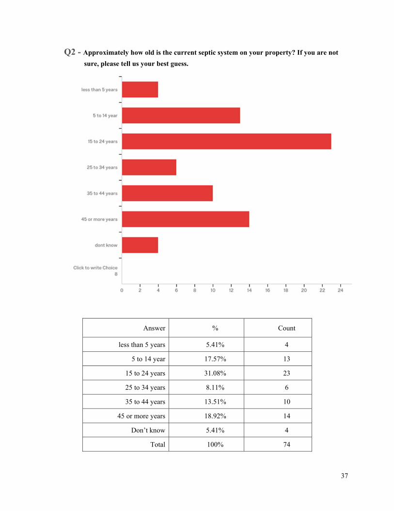
37
Q2 - Approximately how old is the current septic system on your property? If you are not
sure, please tell us your best guess.
Answer % Count
less than 5 years 5.41% 4
5 to 14 year 17.57% 13
15 to 24 years 31.08% 23
25 to 34 years 8.11% 6
35 to 44 years 13.51% 10
45 or more years 18.92% 14
Don’t know 5.41% 4
Total 100% 74
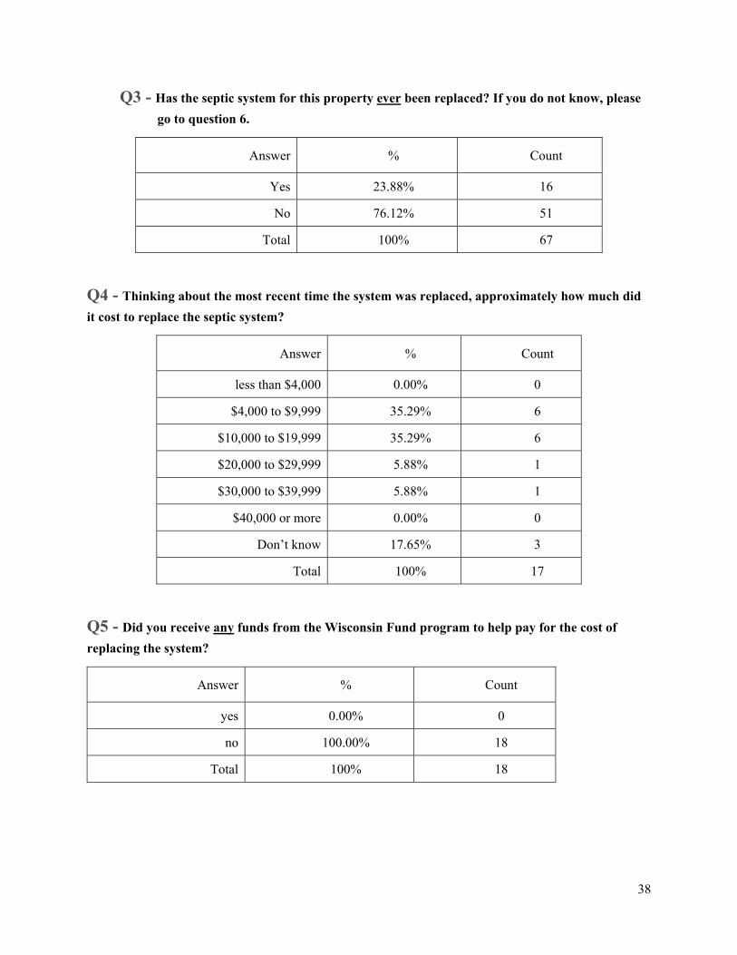
38
Q3 - Has the septic system for this property ever been replaced? If you do not know, please
go to question 6.
Answer % Count
Yes 23.88% 16
No 76.12% 51
Total 100% 67
Q4 - Thinking about the most recent time the system was replaced, approximately how much did
it cost to replace the septic system?
Answer % Count
less than $4,000 0.00% 0
$4,000 to $9,999 35.29% 6
$10,000 to $19,999 35.29% 6
$20,000 to $29,999 5.88% 1
$30,000 to $39,999 5.88% 1
$40,000 or more 0.00% 0
Don’t know 17.65% 3
Total 100% 17
Q5 - Did you receive any funds from the Wisconsin Fund program to help pay for the cost of
replacing the system?
Answer % Count
yes 0.00% 0
no 100.00% 18
Total 100% 18

39
Q6 - Have you ever used any of the following methods to maintain your septic system? Have
you…
Question more
than 1x per year
~1x per year
every 2 to 4
years
every 5 to 10 years
never Total
had OWTS inspected
0.00% 0 8.82% 6 73.53% 50 7.35% 5 10.29% 7 68
had OWTS pumped out
6.85% 5 6.85% 5 78.08% 57 4.11% 3 4.11% 3 73
reduced kitchen waste
76.47% 52 1.47% 1 0.00% 0 0.00% 0 22.06% 15 68

40
reduced household cleaners
67.65% 46 1.47% 1 2.94% 2 0.00% 0 27.94% 19 68
reduced pharma/personal care products
73.91% 51 0.00% 0 0.00% 0 0.00% 0 26.09% 18 69
added chemicals and biological compounds
18.57% 13 4.29% 3 7.14% 5 1.43% 1 68.57% 48 70
other? 8.33% 1 0.00% 0 0.00% 0 0.00% 0 91.67% 11 12
Q7 - Thinking about the past 5 years, what is the average yearly maintenance cost of your
septic system? Please do not include the cost of replacing the system.
Answer % Count
less than $250 per year 80.82% 59
$250 to $499 per year 15.07% 11
$500 to $749 1.37% 1
$750 to $999 2.74% 2
$1,000 or more 0.00% 0
Total 100% 73
Q8 - Does anyone in your household drink water from a private well located on your property?
Answer % Count
yes 94.59% 70
no 5.41% 4
Total 100% 74

41
Q9 - What is the approximate depth of this private well?
Answer % Count
less than 40 feet 5.71% 4
40 to 99 feet 22.86% 16
100 to 149 feet 15.71% 11
150 to 249 feet 21.43% 15
250 or more 4.29% 3
Don’t know 30.00% 21
Total 100% 70
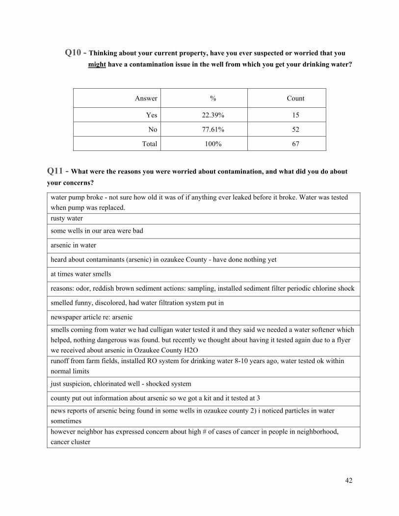
42
Q10 - Thinking about your current property, have you ever suspected or worried that you
might have a contamination issue in the well from which you get your drinking water?
Answer % Count
Yes 22.39% 15
No 77.61% 52
Total 100% 67
Q11 - What were the reasons you were worried about contamination, and what did you do about
your concerns?
water pump broke - not sure how old it was of if anything ever leaked before it broke. Water was tested
when pump was replaced.
rusty water
some wells in our area were bad
arsenic in water
heard about contaminants (arsenic) in ozaukee County - have done nothing yet
at times water smells
reasons: odor, reddish brown sediment actions: sampling, installed sediment filter periodic chlorine shock
smelled funny, discolored, had water filtration system put in
newspaper article re: arsenic
smells coming from water we had culligan water tested it and they said we needed a water softener which
helped, nothing dangerous was found. but recently we thought about having it tested again due to a flyer
we received about arsenic in Ozaukee County H2O
runoff from farm fields, installed RO system for drinking water 8-10 years ago, water tested ok within
normal limits
just suspicion, chlorinated well - shocked system
county put out information about arsenic so we got a kit and it tested at 3
news reports of arsenic being found in some wells in ozaukee county 2) i noticed particles in water
sometimes
however neighbor has expressed concern about high # of cases of cancer in people in neighborhood,
cancer cluster
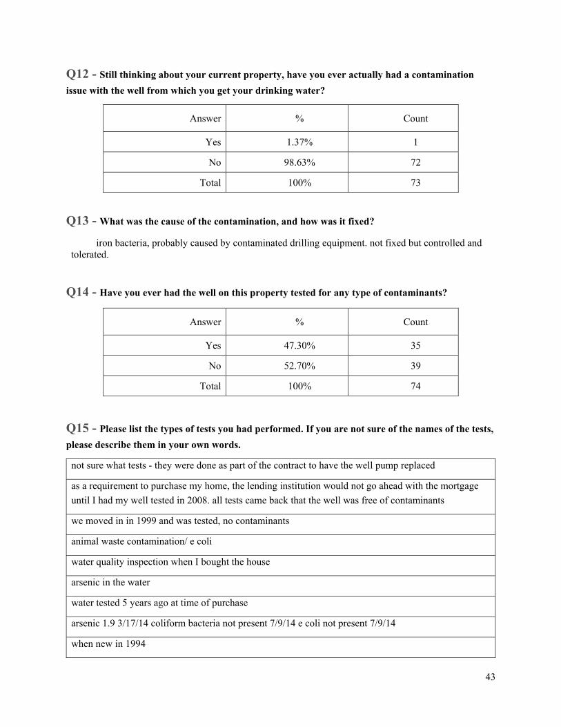
43
Q12 - Still thinking about your current property, have you ever actually had a contamination
issue with the well from which you get your drinking water?
Answer % Count
Yes 1.37% 1
No 98.63% 72
Total 100% 73
Q13 - What was the cause of the contamination, and how was it fixed?
iron bacteria, probably caused by contaminated drilling equipment. not fixed but controlled and tolerated.
Q14 - Have you ever had the well on this property tested for any type of contaminants?
Answer % Count
Yes 47.30% 35
No 52.70% 39
Total 100% 74
Q15 - Please list the types of tests you had performed. If you are not sure of the names of the tests,
please describe them in your own words.
not sure what tests - they were done as part of the contract to have the well pump replaced
as a requirement to purchase my home, the lending institution would not go ahead with the mortgage
until I had my well tested in 2008. all tests came back that the well was free of contaminants
we moved in in 1999 and was tested, no contaminants
animal waste contamination/ e coli
water quality inspection when I bought the house
arsenic in the water
water tested 5 years ago at time of purchase
arsenic 1.9 3/17/14 coliform bacteria not present 7/9/14 e coli not present 7/9/14
when new in 1994

44
arsenic
standard test for purchase of home done in 2008
sent in water samples 2 years ago
fluoride screen, nitrate screen, total coliform, arsenic
done by well digger, water tested by the county
arsenic
when we first moved in and built, the water was tested. not sure for what type of tests.
just bought the house and as part of the sale the well was tested for several things
culligan and not sure. when we refinanced a loan we took a sample to Kemps Dairy where they would
test it, had to collect the water a certain way. cant remember.
unknown which test were performed but they were conducted as part of the purchas of the property in
2009
coliform bacteria e coli nitrates arsenic
testing done by culligan
had water tested annually because of daycare business
did a replacement of the pump check valve - they did whatever is required test and the tests came back
fine - did this about 3 months ago in January
tested when we bought the house in 2007
county tested when we bought it
see above for arsenic results, they did a test when they 1st put it in but i don't know what for - probably
e coli and hardness
the well water was tested when we purchased the house in march 1994 - part of the closing procedures
fecal, nitrates, e. coli
I have had the water tested for arsenic and for other contaminants dangerous to health, but I don't
remember what they were called
prior to purchase of home, coliform, NO3, also self done test meausres of pH, hardness, and iron
coliform bacteria = not present escherichia coli = not present nitrate = 1.87 mg/l arsnic = 5.5 ug/l tests
completed on 8/22/2016
we recently purchased the property during the course of the process there were several tests done to the
water. I assume one of them was for the water in well.
not sure what tests. at time of build and installation the well was tested nearly 23 years ago.
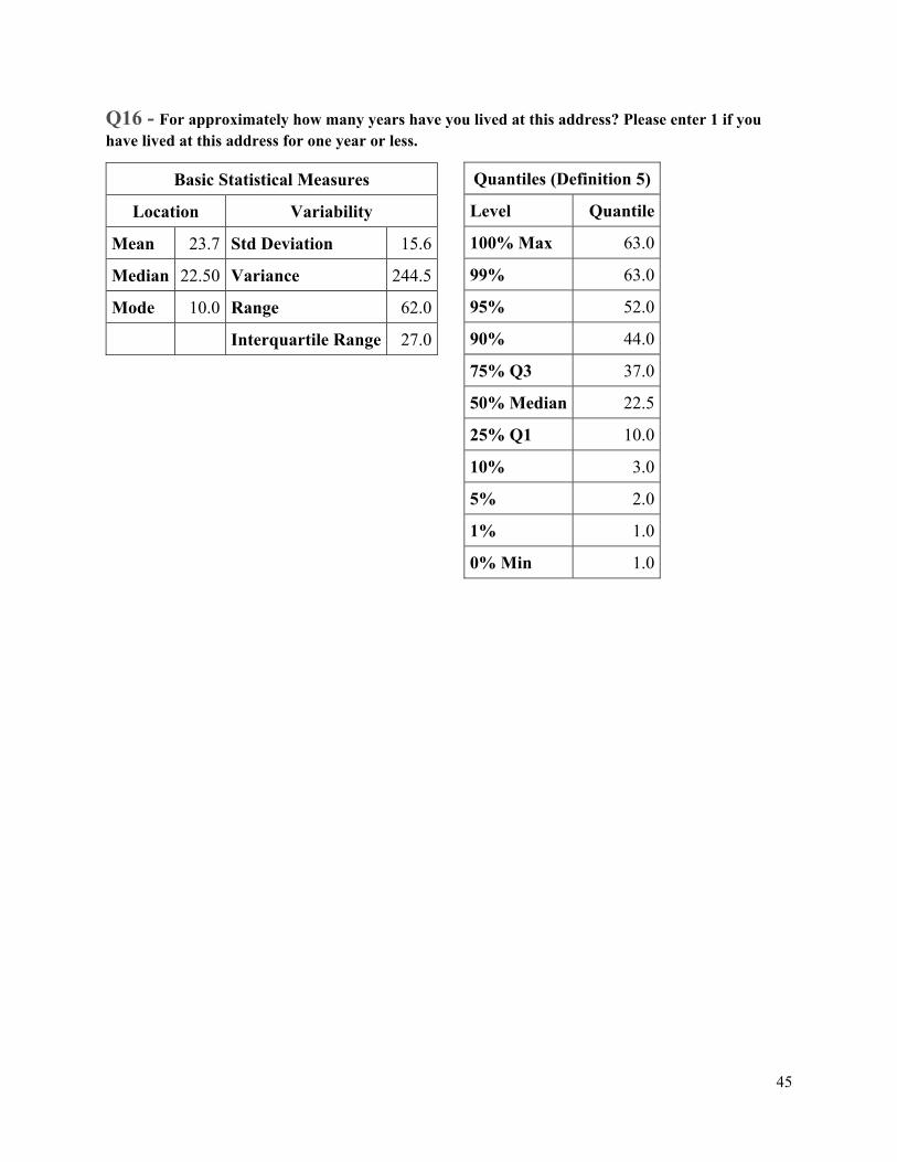
45
Q16 - For approximately how many years have you lived at this address? Please enter 1 if you have lived at this address for one year or less.
Basic Statistical Measures
Location Variability
Mean 23.7 Std Deviation 15.6
Median 22.50 Variance 244.5
Mode 10.0 Range 62.0
Interquartile Range 27.0
Quantiles (Definition 5)
Level Quantile
100% Max 63.0
99% 63.0
95% 52.0
90% 44.0
75% Q3 37.0
50% Median 22.5
25% Q1 10.0
10% 3.0
5% 2.0
1% 1.0
0% Min 1.0

46
Q17 - In what year was this home built? If you are not sure, please provide your best estimate.
*NOTE: For analysis purposes we generated self-reported home age by subtracting responses from 2017
Basic Statistical Measures
Location Variability
Mean 53.2 Std Deviation 40.0
Median 43.0 Variance 1604
Mode 42.0 Range 144.0
Interquartile Range 39.0
Quantiles (Definition 5)
Level Quantile
100% Max 152
99% 152
95% 142
90% 122
75% Q3 62
50% Median 43
25% Q1 23
10% 13
5% 11
1% 8
0% Min 8
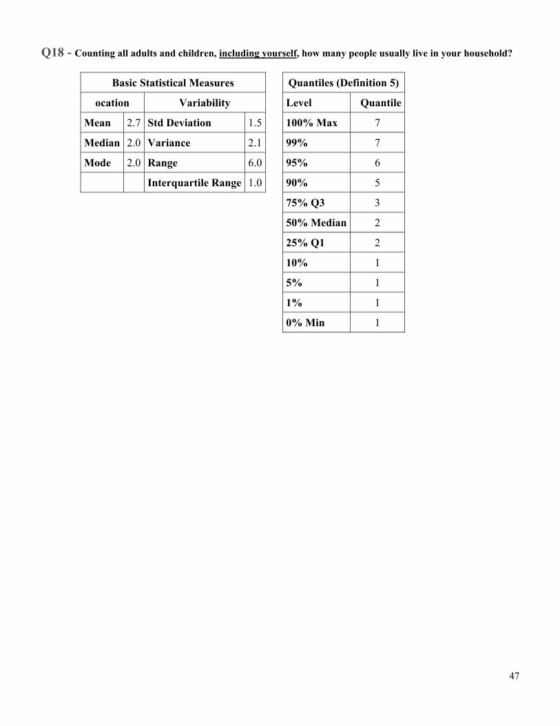
47
Q18 - Counting all adults and children, including yourself, how many people usually live in your household?
Basic Statistical Measures
ocation Variability
Mean 2.7 Std Deviation 1.5
Median 2.0 Variance 2.1
Mode 2.0 Range 6.0
Interquartile Range 1.0
Quantiles (Definition 5)
Level Quantile
100% Max 7
99% 7
95% 6
90% 5
75% Q3 3
50% Median 2
25% Q1 2
10% 1
5% 1
1% 1
0% Min 1

48
Q19 - Approximately how many months do you live in the home each year? Please answer from 1
month up to 12 months.
Q20 - Would you be willing to participate in a water quality sampling project that will test your
well AT NO COST TO YOU for typical contaminants such as Nitrates, Nitrites, E-Coli,
Enterococci, dissolved solids or other contaminants found in some of Wisconsin’s private wells?
Answer % Count
Yes 83.78% 62
No 16.22% 12
Total 100% 74
Basic Statistical Measures
Location Variability
Mean 11.6 Std Deviation 1.7
Median 12.0 Variance 2.8
Mode 12.0 Range 9.0
Interquartile Range 0
Quantiles (Definition 5)
Level Quantile
100% Max 12
99% 12
95% 12
90% 12
75% Q3 12
50% Median 12
25% Q1 12
10% 12
5% 7
1% 3
0% Min 3
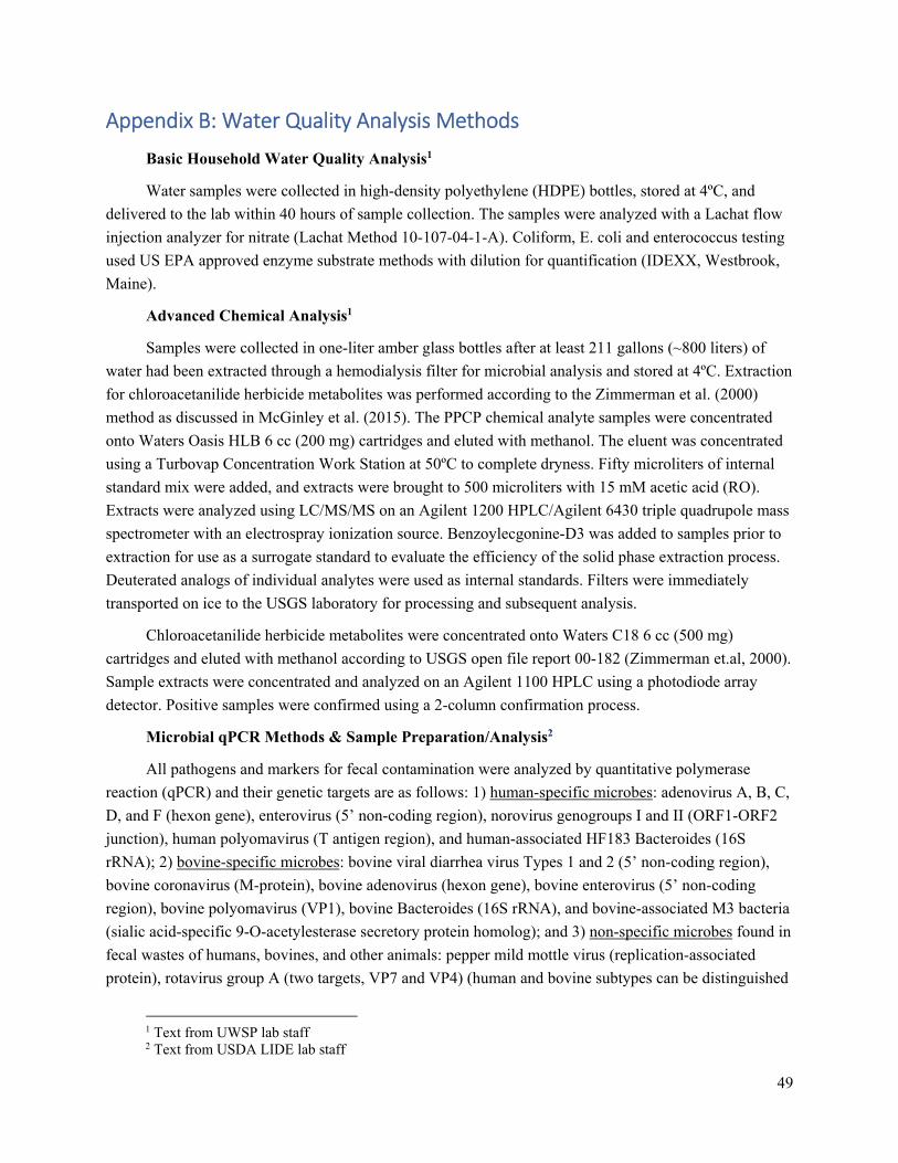
49
Appendix B: Water Quality Analysis Methods
Basic Household Water Quality Analysis1
Water samples were collected in high-density polyethylene (HDPE) bottles, stored at 4ºC, and
delivered to the lab within 40 hours of sample collection. The samples were analyzed with a Lachat flow
injection analyzer for nitrate (Lachat Method 10-107-04-1-A). Coliform, E. coli and enterococcus testing
used US EPA approved enzyme substrate methods with dilution for quantification (IDEXX, Westbrook,
Maine).
Advanced Chemical Analysis1
Samples were collected in one-liter amber glass bottles after at least 211 gallons (~800 liters) of
water had been extracted through a hemodialysis filter for microbial analysis and stored at 4ºC. Extraction
for chloroacetanilide herbicide metabolites was performed according to the Zimmerman et al. (2000)
method as discussed in McGinley et al. (2015). The PPCP chemical analyte samples were concentrated
onto Waters Oasis HLB 6 cc (200 mg) cartridges and eluted with methanol. The eluent was concentrated
using a Turbovap Concentration Work Station at 50ºC to complete dryness. Fifty microliters of internal
standard mix were added, and extracts were brought to 500 microliters with 15 mM acetic acid (RO).
Extracts were analyzed using LC/MS/MS on an Agilent 1200 HPLC/Agilent 6430 triple quadrupole mass
spectrometer with an electrospray ionization source. Benzoylecgonine-D3 was added to samples prior to
extraction for use as a surrogate standard to evaluate the efficiency of the solid phase extraction process.
Deuterated analogs of individual analytes were used as internal standards. Filters were immediately
transported on ice to the USGS laboratory for processing and subsequent analysis.
Chloroacetanilide herbicide metabolites were concentrated onto Waters C18 6 cc (500 mg)
cartridges and eluted with methanol according to USGS open file report 00-182 (Zimmerman et.al, 2000).
Sample extracts were concentrated and analyzed on an Agilent 1100 HPLC using a photodiode array
detector. Positive samples were confirmed using a 2-column confirmation process.
Microbial qPCR Methods & Sample Preparation/Analysis2
All pathogens and markers for fecal contamination were analyzed by quantitative polymerase
reaction (qPCR) and their genetic targets are as follows: 1) human-specific microbes: adenovirus A, B, C,
D, and F (hexon gene), enterovirus (5’ non-coding region), norovirus genogroups I and II (ORF1-ORF2
junction), human polyomavirus (T antigen region), and human-associated HF183 Bacteroides (16S
rRNA); 2) bovine-specific microbes: bovine viral diarrhea virus Types 1 and 2 (5’ non-coding region),
bovine coronavirus (M-protein), bovine adenovirus (hexon gene), bovine enterovirus (5’ non-coding
region), bovine polyomavirus (VP1), bovine Bacteroides (16S rRNA), and bovine-associated M3 bacteria
(sialic acid-specific 9-O-acetylesterase secretory protein homolog); and 3) non-specific microbes found in
fecal wastes of humans, bovines, and other animals: pepper mild mottle virus (replication-associated
protein), rotavirus group A (two targets, VP7 and VP4) (human and bovine subtypes can be distinguished
1 Text from UWSP lab staff 2 Text from USDA LIDE lab staff
50
by P and G subtyping if necessary), Enterococcus species (23S rRNA), Campylobacter jejuni (mapA
gene), Salmonella species (invA gene and ttr locus), enterohemorrhagic E. coli (eae gene and stx 1 and stx
2).
All listed assays were conducted on groundwater samples in the USGS laboratory. Quantification
was by hydrolysis probes (i.e. Taqman) and standard curves created from gblocks® and Ultramer® oligos
(Integrated DNA Technologies, Coralville, IA). Details on qPCR procedures can be found at: Borchardt
et al. 2012, http://dx.doi.org/10.1289/ehp.1104499 Supplemental Material and U.S. EPA Method 1615
www.epa.gov/nerlcwww/documents/Method1615v1_1.pdf. Strict quality assurance and quality control
procedures were followed and PCR inhibitio was measured on every sample. Culture methods (bacteria
and viruses) and nucleic acid sequencing methods were employed as needed to meet study objectives.
Total coliforms and E. coli were analyzed by Quanti-Tray (IDEXX, Westbrook, ME). Cryptosporidium
and Giardia were analyzed by immunofluorescence microscopy using the Merifluor® kit (Meridian
Bioscience Inc. Cincinnati, OH).
A LightCycler® 480 instrument (Roche Diagnostics, Mannheim, Germany) was used to perform
qPCR using the LightCycler 480 Probes Master kit. Fourteen µL of master mix and 6 µL extracted DNA
or cDNA from reverse transcription were combined to produce a 20 µL reaction volume. Assays were
completed for qPCR, including Primer (Integrated DNA Technology, Coralville, IA) and hydrolysis
probe (TIB Molbiol, Berlin, Germany) concentrations. Thermocycling began at 95 °C for 10 min
followed by 45 cycles of 10 s at 95 °C and 1 min at 60 °C with ramp rates of 4.4 and 2.2 °C s-1,
respectively. qPCR was performed in duplicate. If both duplicates were negative the result is reported as
0. If only one was positive, that concentration is reported. If both duplicates were positive, the average is
reported.
Negative controls were included at all processing steps and must exhibit no fluorescence above the
baseline: secondary concentration (backflush solution carried through secondary concentration to qPCR),
nucleic acid extraction (AE buffer extracted with samples), reverse transcription (PCR-grade water
reverse-transcribed with samples; RNA organisms only), and qPCR (PCR-grade water added to master
mix). Positive controls (gBlocks® or Ultramers®; Integrated DNA Technology, Coralville, IA) were
included in each qPCR batch for each target. Modified live virus vaccines (Zoetis Inc., Kalamazoo, MI)
were used for DNA (bovine herpes virus) and RNA (bovine respiratory syncytial virus) extraction
positive controls, with the latter serving also as the reverse transcription positive control.
Quantification cycle (Cq) values were calculated using the second derivative maximum method.
Standard curves were made with gBlocks® or Ultramers® (Integrated DNA Technology, Coralville, IA)
in AE buffer (Qiagen, Valencia, CA) with 0.02% bovine serum albumin (BSA) and were regressed using
the non-linear function provided by the LightCycler 480 software.
Inhibition was evaluated for all samples for both qPCR and reverse transcription-qPCR following
Gibson et al. (2012). Lambda phage DNA or hepatitis G virus armored RNA was spiked into qPCR or
reverse transcription master mix, respectively. Sample template or a 0.02% BSA inhibition control was
added to the master mix, and qPCR or reverse transcription-qPCR was performed as described above.

51
Samples were diluted to attenuate inhibition when the Cq value for the spiked DNA or RNA was greater
than 2 cycles above the inhibition control Cq value, which indicates inhibition (Gibson et al., 2012).

52
Appendix C: Basic Water Quality Results
En
tero
cocc
i M
PN
/100
mls
To
tal C
olif
orm
M
PN
/100
mls
E.
Co
li M
PN
/100
mls
NO
2+N
O3
(N)
m
g/L
Ele
vati
on
OW
TS
Den
sity
Ho
me
Ag
e
Pre
cip
itat
ion
(I
nch
es -
120
H
ou
rs)
UW # LAB #
61201 1700303‐1 <1 1.0 <1 <0.1 785.99 1.95 122 0.53
61202 1700303-2 <1 <1 <1 2.7 885.71 0.09 24 0.53
61203 1700303-3 <1 <1 <1 1.0 852.79 0.74 19 0.53
61204 1700303-4 <1 <1 <1 1.2 850.38 0.84 45 0.53
61205 1700303-5 <1 <1 <1 2.9 864.75 0.74 46 0.53
61206 1700303-6 <1 <1 <1 <0.1 785.37 2.14 117 0.53
61207 1700303-7 <1 <1 <1 <0.1 827.34 0.84 122 0.53
61208 1700303‐8 <1 3.1 <1 <0.1 837.46 0.46 13 0.53
61209 1700303-9 <1 <1 <1 <0.1 788.52 0.46 17 0.53
61210 1700303-10 <1 <1 <1 <0.1 812.42 0.46 24 0.53
61211 1700303-11 <1 <1 <1 <0.1 803.58 0.19 16 0.53
61212 1700303-12 <1 <1 <1 <0.1 811.02 0.19 137 0.53
61213 1700303-13 <1 <1 <1 <0.1 825.88 0.65 62 0.53
61214 1700303-14 <1 <1 <1 <0.1 864.20 0.56 11 0.53
61215 1700303-15 <1 <1 <1 2.5 845.94 0.46 47 0.53
61216 1700303-16 <1 <1 <1 4.7 870.26 0.74 42 0.53
62001 1700324-1 <1 <1 <1 <0.1 855.14 0.09 23 0.66
62002 1700324‐2 <1 70.6 <1 <0.1 867.67 0.19 142 0.66
62003 1700324-3 <1 <1 <1 <0.1 786.68 0.37 63 0.66
62004 1700324-4 <1 <1 <1 <0.1 879.53 0.56 8 0.66
62005 1700324-5 <1 <1 <1 1.1 854.81 0.65 N/A 0.66
62006 1700324-6 <1 <1 <1 <0.1 805.33 0.28 25 0.66
62007 1700324‐7 <1 270.0 <1 <0.1 787.17 0.28 27 0.66
62008 1700324-8 <1 <1 <1 <0.1 797.19 0.46 15 0.66
62009 1700324-9 <1 <1 <1 <0.1 797.03 0.28 23 0.66
62010 1700324-10 <1 <1 <1 <0.1 832.46 0.28 13 0.66
62011 1700324‐11 2.0 9.8 <1 <0.1 788.75 2.32 147 0.66
62012 1700324‐12 <1 5.2 <1 <0.1 794.84 2.32 106 0.66
62013 1700324-13 <1 <1 <1 2.5 827.24 0.37 23 0.66
62014 1700324-14 <1 <1 <1 <0.1 877.53 0.19 112 0.66
62015 1700324-15 <1 <1 <1 0.6 881.69 0.46 24 0.66
62016 1700324-16 <1 <1 <1 <0.1 873.32 0.09 44 0.66
62017 1700324-17 <1 <1 <1 <0.1 889.64 0.46 19 0.66
62018 1700324‐18 11.0 44.8 <1 1.5 881.84 0.37 40 0.66
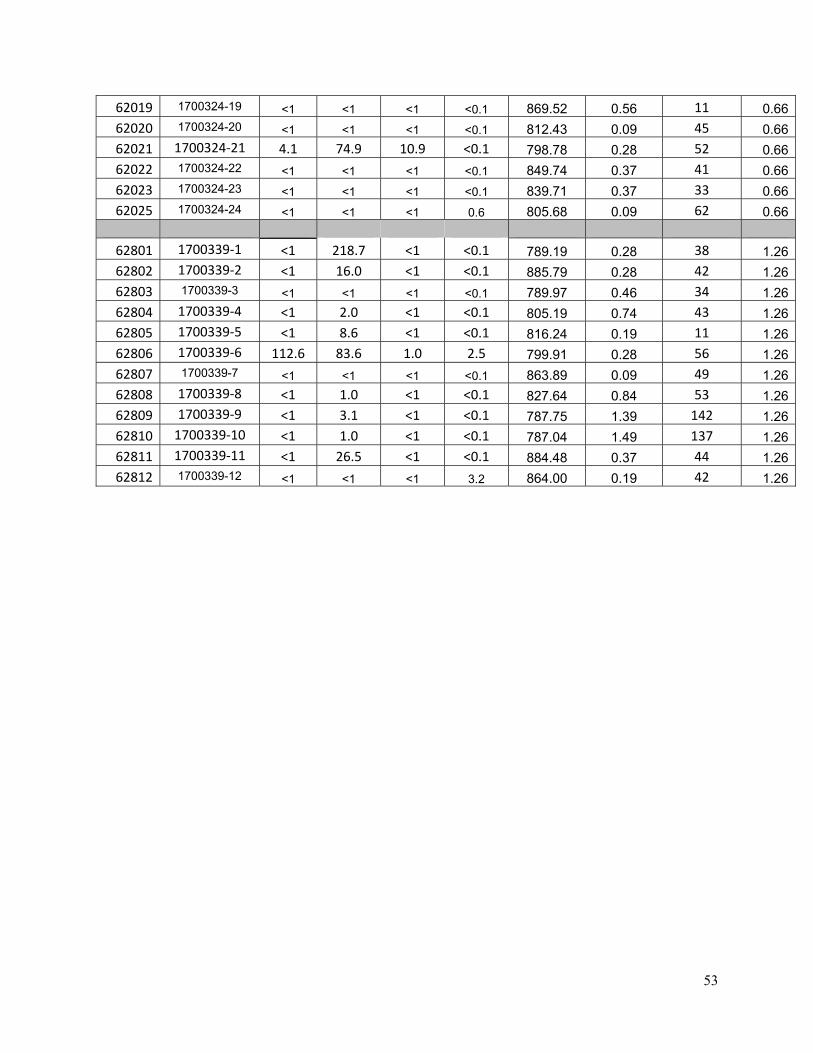
53
62019 1700324-19 <1 <1 <1 <0.1 869.52 0.56 11 0.66
62020 1700324-20 <1 <1 <1 <0.1 812.43 0.09 45 0.66
62021 1700324‐21 4.1 74.9 10.9 <0.1 798.78 0.28 52 0.66
62022 1700324-22 <1 <1 <1 <0.1 849.74 0.37 41 0.66
62023 1700324-23 <1 <1 <1 <0.1 839.71 0.37 33 0.66
62025 1700324-24 <1 <1 <1 0.6 805.68 0.09 62 0.66
62801 1700339‐1 <1 218.7 <1 <0.1 789.19 0.28 38 1.26
62802 1700339‐2 <1 16.0 <1 <0.1 885.79 0.28 42 1.26
62803 1700339-3 <1 <1 <1 <0.1 789.97 0.46 34 1.26
62804 1700339‐4 <1 2.0 <1 <0.1 805.19 0.74 43 1.26
62805 1700339‐5 <1 8.6 <1 <0.1 816.24 0.19 11 1.26
62806 1700339‐6 112.6 83.6 1.0 2.5 799.91 0.28 56 1.26
62807 1700339-7 <1 <1 <1 <0.1 863.89 0.09 49 1.26
62808 1700339‐8 <1 1.0 <1 <0.1 827.64 0.84 53 1.26
62809 1700339‐9 <1 3.1 <1 <0.1 787.75 1.39 142 1.26
62810 1700339‐10 <1 1.0 <1 <0.1 787.04 1.49 137 1.26
62811 1700339‐11 <1 26.5 <1 <0.1 884.48 0.37 44 1.26
62812 1700339-12 <1 <1 <1 3.2 864.00 0.19 42 1.26

54
Appendix D: Advanced Chemical Sourcing Results
Pharmaceuticals and personal care products - parts per trillion (ng/L) W
EA
L La
b #
UW
Sam
plin
g N
umbe
r
Ace
sulfa
me
(art
ifici
al s
wee
tene
r)
Suc
ralo
se (
artif
icia
l sw
eete
ner)
Sac
char
in (
artif
icia
l sw
eete
ner)
Ace
tam
inop
hen
(ana
lges
ic)
Cot
inin
e (n
icot
ine
met
abol
ite)
Caf
fein
e (s
timul
ant)
Par
axan
thin
e (c
affe
ine
met
abol
ite)
Car
bam
azep
ine
(ant
iepi
lept
ic)
Trim
etho
prim
(hu
man
ant
ibio
tic)
Sul
fam
etha
zine
(bo
vine
ant
ibio
tic)
Sul
fam
etho
xazo
le (
hum
an a
ntib
iotic
)
Ven
lafa
xine
(an
tidep
ress
ant)
Tric
losa
n (a
ntim
icro
bial
)
1700480-01 0620-21 <LOD <LOD <LOD <LOD <LOD <LOD <LOD <LOD <LOD <LOD <LOD <LOD <LOD
1700480-02 0620-18 <LOD <LOD <LOD <LOD <LOD <LOD <LOD <LOD <LOD <LOD <LOD <LOD <LOD
1700480-03 0628-04 <LOD <LOD <LOD <LOD <LOD <LOD <LOD <LOD <LOD <LOD <LOD <LOD <LOD
1700480-04 0620-07 15.2 <LOD <LOD <LOD <LOD <LOD <LOD <LOD <LOD <LOD <LOD <LOD <LOD
1700480-05 0620-06 <LOD <LOD <LOD <LOD <LOD <LOD <LOD <LOD <LOD <LOD <LOD <LOD <LOD
1700480-06 0628-03 <LOD <LOD <LOD <LOD <LOD <LOD <LOD <LOD <LOD <LOD <LOD <LOD <LOD
1700480-07 0628-08 11.1 <LOD <LOD <LOD <LOD <LOD <LOD <LOD <LOD <LOD <LOD <LOD <LOD
1700480-08 0620-09 <LOD <LOD <LOD <LOD <LOD <LOD <LOD <LOD <LOD <LOD <LOD <LOD <LOD
1700480-09 0620-17 <LOD <LOD <LOD <LOD <LOD <LOD <LOD <LOD <LOD <LOD <LOD <LOD <LOD
1700480-10 0620-20 <LOD <LOD <LOD <LOD <LOD <LOD <LOD <LOD <LOD <LOD <LOD <LOD <LOD
1700480-11 0612-01 62.3 139.3 <LOD <LOD <LOD <LOD <LOD <LOD <LOD <LOD <LOD <LOD <LOD
1700480-12 0612-07 <LOD 84.9 <LOD <LOD <LOD <LOD <LOD <LOD <LOD <LOD <LOD <LOD <LOD
1700480-13 0612-10 18.7 121.7 <LOD <LOD <LOD <LOD <LOD <LOD <LOD <LOD <LOD <LOD <LOD
1700480-14 0620-19 <LOD <LOD <LOD <LOD <LOD <LOD <LOD <LOD <LOD <LOD <LOD <LOD <LOD
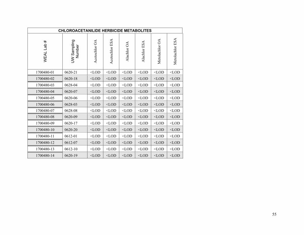
55
CHLOROACETANILIDE HERBICIDE METABOLITES
WE
AL
Lab
#
UW
Sam
plin
g N
umbe
r
Ace
toch
lor
OA
Ace
toch
lor
ESA
Ala
chlo
r O
A
Ala
chlo
r E
SA
Met
olac
hlor
OA
Met
olac
hlor
ESA
1700480-01 0620-21 <LOD <LOD <LOD <LOD <LOD <LOD
1700480-02 0620-18 <LOD <LOD <LOD <LOD <LOD <LOD
1700480-03 0628-04 <LOD <LOD <LOD <LOD <LOD <LOD
1700480-04 0620-07 <LOD <LOD <LOD <LOD <LOD <LOD
1700480-05 0620-06 <LOD <LOD <LOD <LOD <LOD <LOD
1700480-06 0628-03 <LOD <LOD <LOD <LOD <LOD <LOD
1700480-07 0628-08 <LOD <LOD <LOD <LOD <LOD <LOD
1700480-08 0620-09 <LOD <LOD <LOD <LOD <LOD <LOD
1700480-09 0620-17 <LOD <LOD <LOD <LOD <LOD <LOD
1700480-10 0620-20 <LOD <LOD <LOD <LOD <LOD <LOD
1700480-11 0612-01 <LOD <LOD <LOD <LOD <LOD <LOD
1700480-12 0612-07 <LOD <LOD <LOD <LOD <LOD <LOD
1700480-13 0612-10 <LOD <LOD <LOD <LOD <LOD <LOD
1700480-14 0620-19 <LOD <LOD <LOD <LOD <LOD <LOD

56
Appendix E: Advanced Microbial Sourcing Results
Human‐Specific quantitative polymerase chain reaction (qPCR) Analysis Sample ID
Collection Date
LIMS ID
Aden
ovirus A
Aden
ovirus B
Aden
ovirus C,D,F
Enterovirus
Hep
atitis A virus
Human
Bacteroides
Human
polyomavirus
GI n
orovirus
GII norovirus
Microorganism concentrations (genomic copies L‐1)
0612‐01 9/25/17 104741 0 0 0 0 0 0 0 0 0
0612‐07 9/25/17 104750 0 0 0 0 0 0 0 0 0
0612‐10 9/25/17 104747 0 0 0 0 0 0 0 0 0
0620‐06 9/23/17 104744 0 0 0 0 0 0 0 0 0
0620‐07 9/23/17 104746 0 0 0 0 0 0 0 0 0
0620‐09 9/24/17 104743 0 0 0 0 0 0 0 0 0
0620‐17 9/24/17 104740 0 0 0 0 0 0 0 0 0
0620‐18 9/23/17 104748 0 0 0 0 0 0 0 0 0
0620‐19 9/25/17 104745 0 0 0 0 0 0 0 0 0
0620‐20 9/24/2017 104742 0 0 0 0 0 0 0 0 0
0620‐21 9/23/2017 104749 0 0 0 0 0 0 0 0 0
0628‐03 9/24/2017 104739 0 0 0 0 0 0 0 0 0
0628‐04 9/23/2017 104751 0 0 0 0 0 0 0 0 0
0628‐08 9/24/2017 104752 0 0 0 0 0 0 0 0 0

57
Bovine‐Specific quantitative polymerase chain reaction (qPCR) Analysis
Sample ID
Collection Date
LIMS ID
Bovine Ba
cteroide
s
Bovine polyomavirus
Bacteroide
s‐like Cow M
2
Bacteroide
s‐like Cow M
3
Microorganism concentrations (genomic copies L‐1)
0612‐01 9/25/2017 104741 0 0 0 0
0612‐07 9/25/2017 104750 0 0 0 0
0612‐10 9/25/2017 104747 0 0 0 0
0620‐06 9/23/2017 104744 0 0 0 0
0620‐07 9/23/2017 104746 0 0 0 0
0620‐09 9/24/2017 104743 0 0 0 0
0620‐17 9/24/2017 104740 0 0 0 0
0620‐18 9/23/2017 104748 0 0 0 0
0620‐19 9/25/2017 104745 0 0 0 0
0620‐20 9/24/2017 104742 0 0 0 0
0620‐21 9/23/2017 104749 0 0 0 0
0628‐03 9/24/2017 104739 0 0 0 0
0628‐04 9/23/2017 104751 0 0 0 0
0628‐08 9/24/2017 104752 0 0 0 0

58
Non‐Specific quantitative polymerase chain reaction (qPCR) Analysis
Sample ID
Collection Date
LIMS ID
Campyloba
cter jejuni
Cryptosporidium
Enterohem
orrhagic E. coli
(eae
gen
e)
Enterohem
orrhagic E. coli
(stx1 gene)
Enterohem
orrhagic E. coli
(stx2 gene)
Giardia group B
Pep
per m
ild m
ottle virus
Rotavirus (NSP
3)
Rotavirus (VP7)
Salm
onella (invA gene)
Salm
onella (ttr g
ene)
Microorganism concentrations (genomic copies L‐1)
0612‐01 9/25/2017 104741 0 0 0 0 0 0 0 0 0 0 0
0612‐07 9/25/2017 104750 0 0 0 0 0 0 0 0 0 0 0
0612‐10 9/25/2017 104747 0 0 0 0 0 0 0 0 0 0 0
0620‐06 9/23/2017 104744 0 0 0 0 0 0 0 0 0 0 0
0620‐07 9/23/2017 104746 0 0 0 0 0 0 0 0 0 0 0
0620‐09 9/24/2017 104743 0 0 0 0 0 0 0 0 0 0 0
0620‐17 9/24/2017 104740 0 0 0 0 0 0 0 0 0 0 0
0620‐18 9/23/2017 104748 0 0 0 0 0 0 0 0 0 0 0
0620‐19 9/25/2017 104745 0 0 0 0 0 0 0 0 0 0 0
0620‐20 9/24/2017 104742 0 0 0 0 0 0 0 0 0 0 0
0620‐21 9/23/2017 104749 0 0 0 0 0 0 0 0 0 0 0
0628‐03 9/24/2017 104739 0 0 0 0 0 0 0 0 0 0 0
0628‐04 9/23/2017 104751 0 0 0 0 0 0 0 0 0 0 0
0628‐08 9/24/2017 104752 0 0 0 0 0 0 0 0 0 0 0

59
Appendix F: Residential Zoning Policy Inventory
Township Minimum Lot Size Unit of Analysis District Classification
Other Language
Belgium 0.67 DUs per net acre or R‐1 Single Family Only only
2.13F) Private Sewer and Water. The dimension and area of all lots and parcels shall be sufficient to accommodate the use of a private onsite wastewater treatment system (POWTS), designed in accordance with Chapters SPS 383 and 385 of the Wisconsin Administrative Code and Chapter IX, “Sanitation and Health,” of the Ozaukee County Code of Ordinances, and a private water supply system (well) in compliance with Chapter NR 812 of the Wisconsin Administrative Code.
1 DU per 1.5 acres of lot area
Cedarburg 80,000 Square feet per DU R‐1 Single Family Chapter 267: Onsite Sewage Disposal Restricted Holding Tanks Only 40,000 Square feet per DU R‐2 & R‐3 Single
Family
Fredonia 3 Acres per DU R‐1 Single Family The R‐1 District is intended to provide for single‐family development at densities not to exceed 0.33 dwelling units per net acre, served by on‐site soil absorption sanitary sewerage systems (septic tanks) and private wells.
1 Acres per DU R‐2 Single Family The R‐2 District is intended to provide for single‐family residential development at densities not to exceed one dwelling unit per acre, served by on‐site soil absorption sanitary sewerage systems (septic tanks) and private wells.
Grafton 5 Acres per DU R‐1 Single Family Health and Sanitation, Chapter 4 – Holding Tanks Only
3 Acres per DU R‐2 Single Family
1 Acres per DU R‐3 Single Family
40,000 Square feet RM‐1 Multi‐Family
2 Acres per DU R‐Tr Transitional

60
Port Washington
0.75 Acres per DU ACS‐1 Ag Conservation Subdivision
§ 340‐15. Land Suitability A) Private sewer and water. In any district where public sewer service is not available, the width and area of all lots shall be sufficient to permit the use of an on‐site soil absorption sewage system or other appropriate means, designed in accordance with the Wisconsin Administrative Code.
0.75 Acres per DU R‐1 Residential
1 Acres per DU R‐2 Residential
1.33 Acres per DU R‐3 Residential
Saukville 5 Acres per DU A‐1, A‐2, A‐3, A‐4 General Agriculture