eugm 2011 | darchy | deployment & use of east within sanofi r & d
TRANSCRIPT

1
Deployment and use of East within SANOFI R&D
Loïc Darchy Biostatistics Department, SANOFI R&D
UGM CYTEL East
Paris, October 14, 2011

2
CYTEL : Get the right direction !
EAST
SOUTH
NORTH
WEST
COMPASS
3
Outline
Needs Why EAST ? Licence & deployment model within
SANOFI R&D Main applications within SANOFI R&D General statistical framework used in
East A few points for discussion Lessons learnt
4
NEEDS
WE NEED a reference (*), powerful and user-friendly tool for: Power / sample size calculations Designing, simulating, monitoring and analyzing
group sequential designs Implementing adaptive design features such as
interim sample size revision Importance of having:
a powerful simulation engine nice / numerous graphical interfaces a comprehensive & concise user’s manual
(*) with regard to Scientific Community & Health Authorities
5
Why EAST ?
Only a few alternatives Internal development
Validation issues (vis-à-vis FDA, EMA…) Maintenance issues BUT… core programs would be relatively easy to
develop in-house considering that it is rare to perform more than 2 interim analyses
Other software products: AddPlan, older products like PEST
6
Licence & deployment model within SANOFI R&D
Licence model PC installation from 1 CD-Rom installation disk with
a limited number of copies of the software (x copies for East Standard, y<x copies for East Advanced)
Each installation has access to the full software and documentation
East activated for use until one year from the Agreement date
Deployment model Copies of the software distributed across main R&D
sites according to needs 1 key SANOFI user’s contact for CYTEL

7
Main applications within SANOFI R&D 1/4
SCHEMATICALLY: The most common application is (by far) the design &
simulation of group sequential designs E.g. oncology trials, cardiovascular or diabetes prevention
trials, … A well known and recognized methodology
East may also be used once in a while to perform sample size calculations in particular for time-to-event endpoints
Surprisingly: Monitoring module is being rarely used in practice Analysis (i.e. so called stage-wise adjusted analysis) module
has never been run on real case studies !
8
Main applications within SANOFI R&D 2/4
Monitoring module Mainly used at design stage to illustrate scenarios which will
lead to stop the trial (for efficacy and/or futility) Rarely used to monitor a real trial Reasons:
Licensing & training issues with independent statistical centers and/or DMC statisticians
Stopping boundaries are generally pre-defined in the protocol (expressed in nominal significance levels or Z-statistics) and are then used as such
However there are potential issues when deviating from the initial schedule of interim analyses (but correct stopping boundaries can easily be re-calculated with East and forwarded to people who are in charge of interim analyses)
Conditional power calculations can easily be conducted outside East
9
Main applications within SANOFI R&D 3/4
Analysis module The stage-wise (*) adjusted analysis (as proposed by East) is
never used In practice it is replaced by a more classical analysis (and
easily feasible with SAS): non-adjusted p-value naive treatment effect estimate confidence interval based on the adjusted(**) nominal significance
level) which provides rather similar results for most commonly used designs with 1 or 2 interim analyses
However, this naïve approach slightly overestimates the treatment effect
WARNING: bias might not be negligible with aggressive α-spending functions like Pocock and/or repeated interim analyses
(**) according to the pre-defined α-spending function
(*) stage-wise ordering of the sample space
10
Main applications within SANOFI R&D 4/4
Analysis module (continued) Example: 2 equally spaced interim analyses, α=0.025 (one-sided), 1-
β=0.9, Pocock boundaries, interim effect size estimate = 2/3 of expected effect size Δ at each look naïve effect size estimate = 2/3 Δ versus median-unbiased stage-
wise adjusted effect size = 0.935 x 2/3 Δ over-bias of ~ 7% with naïve estimate
versus 0.990 with O’Brien & Fleming Note that the stage-wise adjusted analysis is NOT computed in East:
as long as the maximum information or the rejection of null hypothesis has NOT been achieved (there is no way to specify that the current look is the last one)
at final analysis when the null hypothesis is NOT rejected in presence of futility boundaries (while it is run when the null hypothesis is rejected) BUG ???
THESE ARE SERIOUS LIMITATIONS
11
General statistical framework used in East
TO MAKE IT SHORT: Asymptotic theory with normal distributions Based on score statistics taking advantage of their
(asymptotical) property of independent increments Pre-defined maximum (Fisher) information Imax to be achieved
to meet power requirements Monitoring of the trial according to information scale t (0≤t≤1)
where t=I/ Imax with I = cumulative information at current look Information I depends upon “nuisance” parameters such as
variance, placebo response,… Misjudging nuisance parameters at design stage may
affect the study power Monitoring of nuisance parameters strongly advisable
Stage-wise ordering of sampling space at final analysis resulting in median-unbiased treatment effect size estimate
12
A few points for discussion OR the Prevert’s list (non exhaustive)…
Overriding stopping rules for overwhelming efficacy (e.g. in case of overrunning)
Monitoring extra looks when the maximum information has been exceeded
Inference when the maximum information has been exceeded
Ideal next look position concept Handling of nuisance parameters in conditional power
calculations Repeated confidence intervals Subject Accrual Per Unit Time for time-to-event
endpoints New adaptive setting tools
13
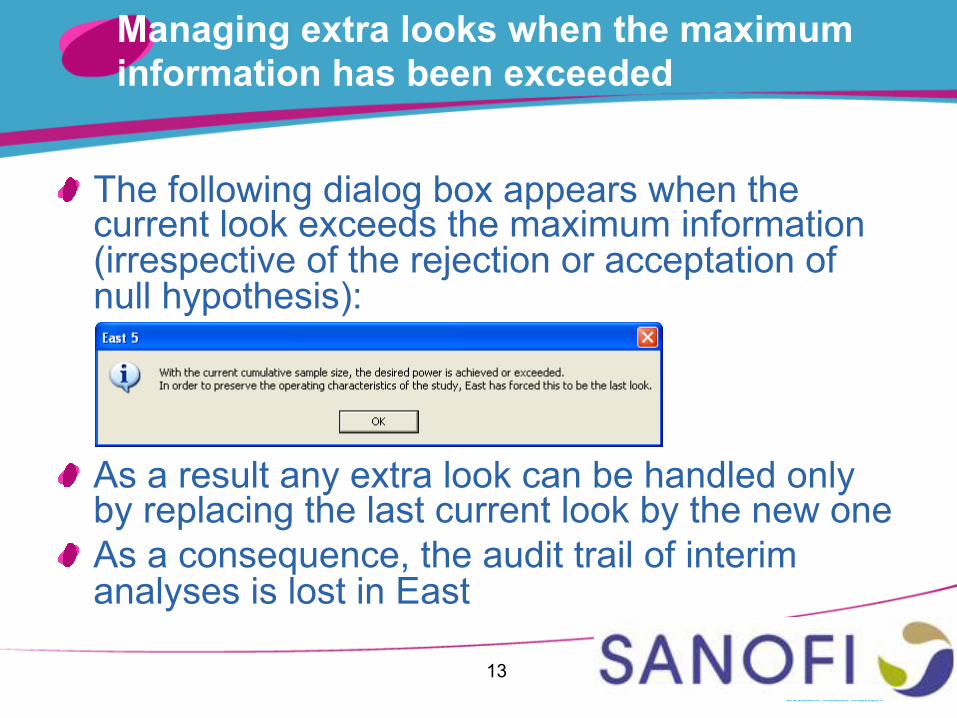
Managing extra looks when the maximum information has been exceeded
The following dialog box appears when the current look exceeds the maximum information (irrespective of the rejection or acceptation of null hypothesis):
As a result any extra look can be handled only by replacing the last current look by the new one
As a consequence, the audit trail of interim analyses is lost in East
14
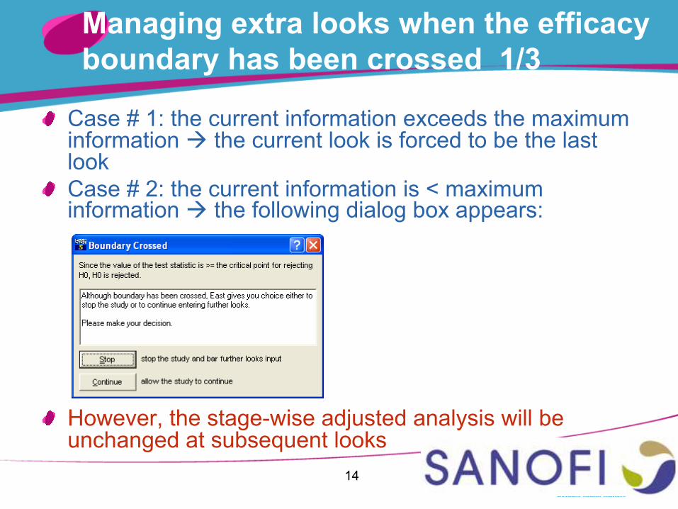
Managing extra looks when the efficacy boundary has been crossed 1/3
Case # 1: the current information exceeds the maximum information the current look is forced to be the last look
Case # 2: the current information is < maximum information the following dialog box appears:
However, the stage-wise adjusted analysis will be unchanged at subsequent looks
15
Managing extra looks when the efficacy boundary has been crossed 2/3
Therefore, the first analysis rejecting H0 is implicitly considered as the reference analysis
Overrunning may / will lead to an extra final analysis but implicitly East positions it as a supportive analysis Certainly the right approach from a pure statistical standpoint But can be challenged by Health Authorities especially in case
of large amount of overrunning Discussion should concentrate on the consistency of
treatment effect estimates across analyses rather than isolated p-values which are poorly informative
In case the sponsor does not want – for any reason - to position the first analysis rejecting H0 as the reference analysis, a (conservative) extended stage-wise inference framework could be proposed as follows (see next slide)
16
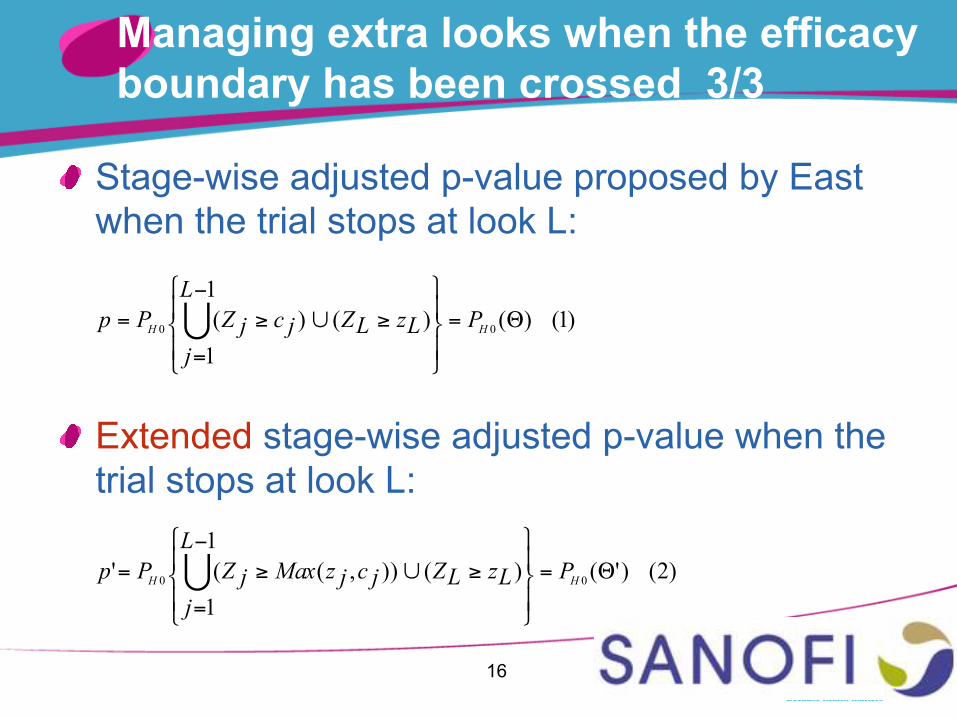
Managing extra looks when the efficacy boundary has been crossed 3/3
Stage-wise adjusted p-value proposed by East when the trial stops at look L:
Extended stage-wise adjusted p-value when the trial stops at look L:
)1()(1
1)()( 00 Θ=
−
=
≥∪≥= HH PL
jLzLZjcjZPp
)2()'(1
1)()),((' 00 Θ=
−
=
≥∪≥= HH PL
jLzLZjcjzMaxjZPp
17
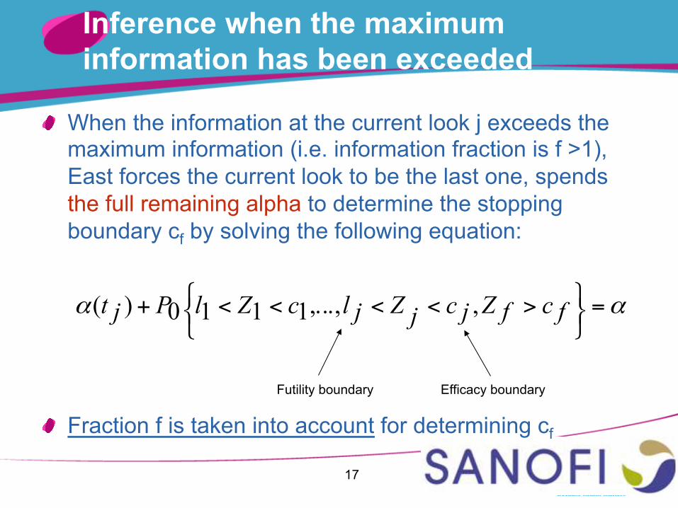
Inference when the maximum information has been exceeded
When the information at the current look j exceeds the maximum information (i.e. information fraction is f >1), East forces the current look to be the last one, spends the full remaining alpha to determine the stopping boundary cf by solving the following equation:
Fraction f is taken into account for determining cf
αα =
><<<<+ fcfZjcjZjlcZlPjt ,,...,1110)(
Futility boundary Efficacy boundary
18
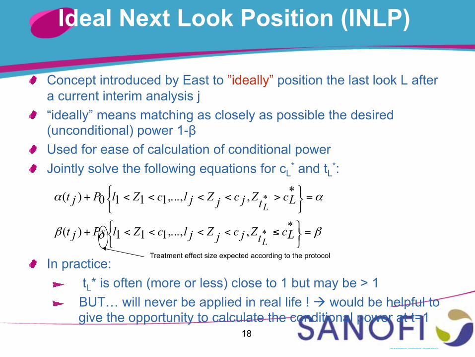
Ideal Next Look Position (INLP)
Concept introduced by East to ”ideally” position the last look L after a current interim analysis j
“ideally” means matching as closely as possible the desired (unconditional) power 1-β
Used for ease of calculation of conditional power Jointly solve the following equations for cL
* and tL*:
In practice: tL* is often (more or less) close to 1 but may be > 1 BUT… will never be applied in real life ! would be helpful to
give the opportunity to calculate the conditional power at t=1
Treatment effect size expected according to the protocol
αα =
><<<<+ *,,...,1110)( * LctZjcjZjlcZlPjt
L
βδβ =
≤<<<<+ *,,...,111)( * LctZjcjZjlcZlPjt
L
19
Handling of nuisance parameters in conditional power calculations 1/3
Conditional power (CP) calculations require to estimate the cumulative information one can get at final analysis or almost equivalently at INLP Note: East provides CP at INLP only
East adjusts its prediction of the cumulative information on current estimate(s) of nuisance parameter(s) For example, for a continuous endpoint, the estimate of
standard deviation at current look is used even if the resulting information at final analysis is less than Imax
Seems a sensible and realistic approach
However, the way to predict the information is NOT documented and is totally rigid in the information-based module (to be used for more complex settings)
20
Handling of nuisance parameters in conditional power calculations 2/3
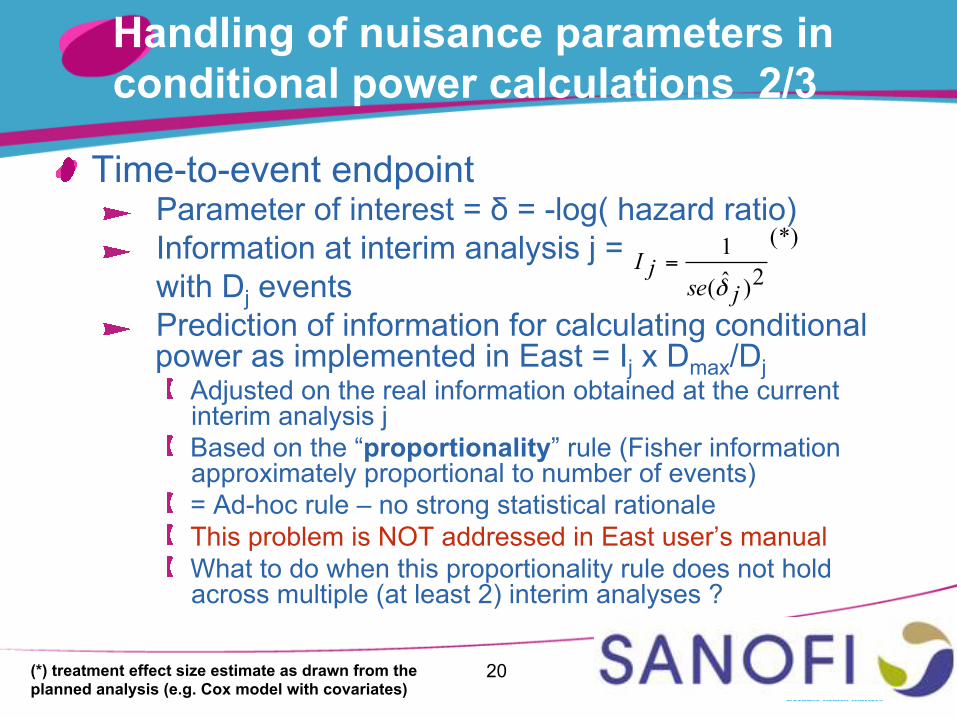
Time-to-event endpoint Parameter of interest = δ = -log( hazard ratio) Information at interim analysis j =
with Dj events Prediction of information for calculating conditional
power as implemented in East = Ij x Dmax/Dj Adjusted on the real information obtained at the current
interim analysis j Based on the “proportionality” rule (Fisher information
approximately proportional to number of events) = Ad-hoc rule – no strong statistical rationale This problem is NOT addressed in East user’s manual What to do when this proportionality rule does not hold
across multiple (at least 2) interim analyses ?
(*)
2)ˆ(
1
jsejI
δ=
(*) treatment effect size estimate as drawn from the planned analysis (e.g. Cox model with covariates)
21
Handling of nuisance parameters in conditional power calculations 3/3
More complex settings Examples: MMRM Analysis, random effects
regression model,… The user must use the East Information-
based module No adjustment is applied by East to predict
the information at final analysis East considers that the pre-defined maximum information will be achieved
Manual adjustments & calculations are to be done by the statistician
22
Repeated confidence intervals 1/3
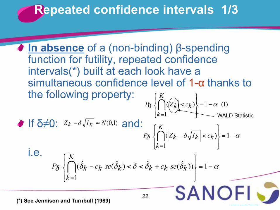
In absence of a (non-binding) β-spending function for futility, repeated confidence intervals(*) built at each look have a simultaneous confidence level of 1-α thanks to the following property:
If δ≠0: and:
i.e.
(*) See Jennison and Turnbull (1989)
)1,0(NkIkZ ≈−δ
αδδ −=
=
<− 11
)(K
kkckIkZP
αδδδδδδ −=
=
+<<− 11
))ˆ(ˆ)ˆ(ˆ(K
kksekckksekckP
)1(11
)(0 α−=
=
<K
kkckZP
WALD Statistic
23
Repeated confidence intervals 2/3
This is a very convenient way (but conservative) to bound the true treatment effect size
Inference is still valid if a stopping boundary is crossed but the DMC nevertheless chooses to keep the study open for further interim looks
24
Repeated confidence intervals 3/3
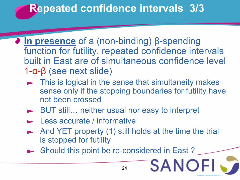
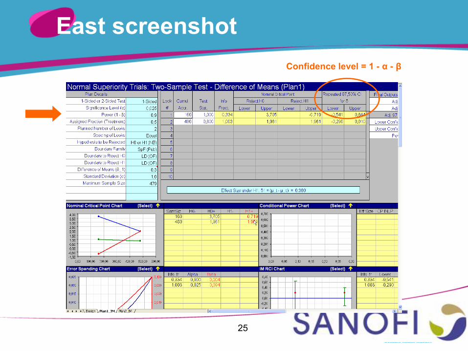
In presence of a (non-binding) β-spending function for futility, repeated confidence intervals built in East are of simultaneous confidence level 1-α-β (see next slide) This is logical in the sense that simultaneity makes
sense only if the stopping boundaries for futility have not been crossed
BUT still… neither usual nor easy to interpret Less accurate / informative And YET property (1) still holds at the time the trial
is stopped for futility Should this point be re-considered in East ?
25
East screenshot Confidence level = 1 - α - β
26
Subject Accrual Per Unit Time
Usually, for a time-to-event endpoint, the required number of events depends only on three parameters α, β and the true hazard ratio r
BUT, in East, it also depends on a fourth parameter which is the « Subject Accrual Per Unit Time »: It is difficult to figure out how this parameter can
influence the number of events This point is NOT addressed in User’s manual
27
New adaptive setting tools
Revision of maximum information based on the observed treatment effect size
Based on CHW methodology and concept of “promising zone”
Missing key information: Unconditional power curve (as a function of the true
hazard ratio) = The only way to properly assess the performance of the design
Comparison with a fixed design (in order to keep things clear and transparent): Efficiency ratio (versus a fixed design) curve (as a function
of the true hazard ratio) when applying the same average sample size
28
Lessons learnt
Group sequential design methodology is well known – granted BUT still offers some statistical challenges
There is still room for clarification (and improvement ?) for
East non-adaptive features
Interim revision of maximum information based on interim treatment effect size estimate: current module NOT fully satisfactory from SANOFI perspective
East customers should try to share (and capitalize on) their
experience & needs need for an efficient network East is globally a mature, robust, efficient and ergonomic
software although there are still a few “gray areas” for the user