eugenio r. m´endez departamento de optica´gea.df.uba.ar/giambiagi/material/mendez_c02.pdf ·...
TRANSCRIPT

Light scattering by randomly rough surfacesEugenio R. Mendez
Departamento de Optica
Outline
• Phenomenological description of the problem.
• Statistical characterization of randomly rough surfaces
• Statistical properties of the scattered field.
• Theoretical approaches:
- The Kirchhoff approximation.
- Perturbation theory and the Rayleigh method.
- Numerical techniques.
• Examples.
• Inverse scattering problems.
- Determination of statistical parameters.
- Profilometry.

Theoretical approaches
Illustrate the theories considering surfaces with 1D roughness. Relevant results for
the 2D case will be mentioned.
Illumination:
Monochromatic plane wave of frequency ω.
Assume also a dependence of the form e−iωt, but not made explicit.
The medium of incidence is vacuum, and the surface is characterized by ε(ω) or,
equivalently, by nc =√ε(ω).
The plane of incidence is the x1x3-plane and the surface is invariant along x2.
Then, the s- and p-polarized components are decoupled:
> p polarization - magnetic field vector H(x1, x3) = (0, H2(x1, x3),0),
> s polarization - electric field vector E(x1, x3) = (0, E2(x1, x3),0).

Theoretical approaches
Scattering by a one-dimensional surface
x1
x3
3 1ζx = (x )
inck
sθ
Es Ep
sck
k
oθEp
Esq
α (q)oα (k)o
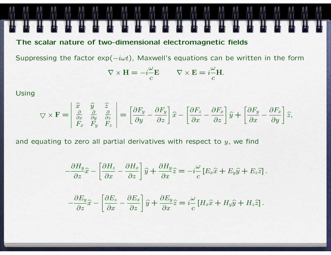
The scalar nature of two-dimensional electromagnetic fields
Suppressing the factor exp(−iωt), Maxwell’s equations can be written in the form
∇×H = −iω
cE ∇× E = i
ω
cH.
Using
5× F =
∣∣∣∣∣∣x y z∂∂x
∂∂y
∂∂z
Fx Fy Fz
∣∣∣∣∣∣ =
[∂Fy
∂y−∂Fy
∂z
]x−
[∂Fz
∂x−∂Fx
∂z
]y+
[∂Fy
∂x−∂Fx
∂y
]z,
and equating to zero all partial derivatives with respect to y, we find
−∂Hy
∂zx−
[∂Hz
∂x−∂Hx
∂z
]y+
∂Hy
∂xz = −i
ω
c[Exx+ Eyy+ Ezz] .
−∂Ey
∂zx−
[∂Ez
∂x−∂Ex
∂z
]y+
∂Ey
∂xz = i
ω
c[Hxx+Hyy+Hzz] .

From these equations we obtain the two independent sets
−∂Ey
∂z= i
ω
cHx
∂Ey
∂x= i
ω
cHz
[∂Hz
∂x−∂Hx
∂z
]= i
ω
cEy,
and
−∂Hy
∂z= −i
ω
cEx
∂Hy
∂x= −i
ω
cEz
[∂Ez
∂x−∂Ex
∂z
]= −i
ω
cHy.
The first set involves only Hx, Hz and Ey.
The second one involves only Ex, Ez, and Hy.
It is then convenient to separate any solution into a linear combination of the two
solutions.

s polarization or Transverse Electric (TE)
Ex = 0, Ez = 0, Hy = 0.
Substituting the first two conditions into the third one we find[∂2Ey
∂x2+∂2Ey
∂z2
]+
(ωc
)2Ey = 0.
This expression shows that the complete field is specified in terms of Ey, which, of
course, satisfies the two dimensional Helmholtz equation.
p polarization or Transverse Magnetic (TM)
Hx = 0, Hz = 0, Ey = 0.
Following similar steps one finds that the complete field is specified in terms of Hy.[∂2Hy
∂x2+∂2Hy
∂z2
]+
(ωc
)2Hy = 0.
Since the surface is one-dimensional, the cases of s and p polarization can be treated
separately.

Example: Perfect conductor with s polarization.
The boundary conditions satisfied by EI(~r) at the interface may be written as
EI(~R) = 0.
We now introduce the Green’s function GI(~r|~r ′) for region I, as a solution of the
equations represented by[∇2 + (ω/c)2
]GI(~r|~r ′) = −4πδ(~r − ~r ′) .
These function may be represented in terms of Hankel functions of the first kind as
follows,
GI(~r|~r ′) = iπH(1)0
(ωc|~r − ~r ′|
).
The Green’s function has the following convenient representation
GI(~r|~r ′) =
∫ ∞
−∞
dk
2π
2πi
α0(k)exp
{ik
(x− x′
)+ iα0(k)
(z − z′
)},
where
α0(kω) =
{ √(ω/c)2 − k2 if k < ω/c,
i√k2 − (ω/c)2 if k > ω/c.

.
Applying Green’s second integral theorem to region I , we obtain∫V
(u∇2v − v∇2u
)dV =
∫Σ
(u∂
∂n−v − v
∂
∂n−u
)dΣ,
where ∂/∂n− is the derivative along the normal to the surface Σ, away from the volume
V . It is convenient to use the derivative in the other direction. That is
∂
∂n= −
∂
∂n−.
Then we find
EI(~r) =1
4π
∫Σ
[(∂
∂nGI(~r|~R)
)EI(~R)−GI(~r|~R)
(∂
∂nEI(~R)
)]dΣ .
The integral can be split into to contributions. One due to the surface, and the other
due to the half-cilinder region. Using the boundary condition we obtain
EI(~r) = EIinc(~r)−
1
4π
∫ ∞
−∞GI(~r|~R)
(∂
∂nEI(~R)
)ds ,
with∂
∂n=
1(1 + (ζ ′(x))2
)1/2
(−ζ(x)
∂
∂x+
∂
∂z
)

The scattering amplitude
Let us consider the scattered field
EIsc(~r) =
−1
4π
∫ ∞
−∞GI(~r|~r′)
F (x′)
φ(x′)ds′ ,
where
F (x′) =
[−ζ(x′)
∂
∂x′+
∂
∂z′
]EI(x′, z′)
∣∣∣∣z′=ζ(x′)
= φ(x)
(∂
∂nEI(~R)
)represents the source function.
Given that
ds′ =(1 +
(ζ ′(x)
)2)dx′ = φ(x′)dx′.
Wih this, the scattered field can be written as
EIsc(~r) =
−1
4π
∫ ∞
−∞GI(~r|~r′)F (x′) dx′ .
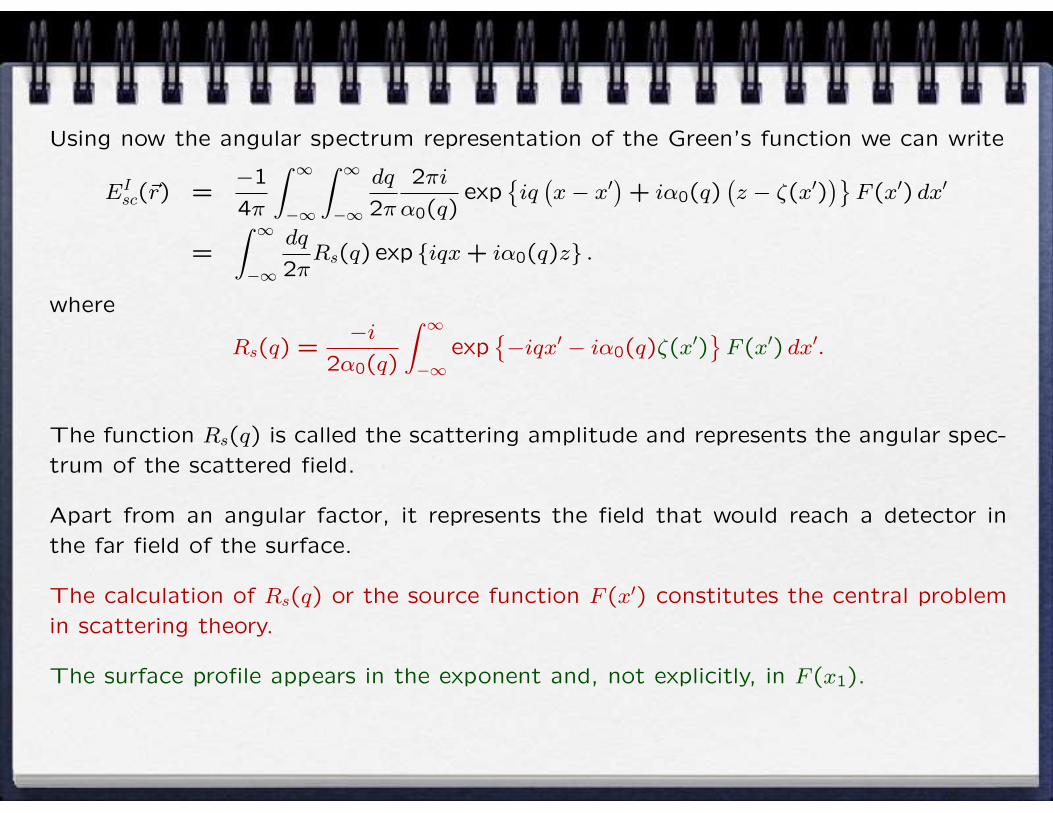
Using now the angular spectrum representation of the Green’s function we can write
EIsc(~r) =
−1
4π
∫ ∞
−∞
∫ ∞
−∞
dq
2π
2πi
α0(q)exp
{iq
(x− x′
)+ iα0(q)
(z − ζ(x′)
)}F (x′) dx′
=
∫ ∞
−∞
dq
2πRs(q) exp {iqx+ iα0(q)z} .
where
Rs(q) =−i
2α0(q)
∫ ∞
−∞exp
{−iqx′ − iα0(q)ζ(x
′)}F (x′) dx′.
The function Rs(q) is called the scattering amplitude and represents the angular spec-
trum of the scattered field.
Apart from an angular factor, it represents the field that would reach a detector in
the far field of the surface.
The calculation of Rs(q) or the source function F (x′) constitutes the central problem
in scattering theory.
The surface profile appears in the exponent and, not explicitly, in F (x1).

The Kirchhoff approximation (locally flat surfaces)
In the KA one assumes that the source functions for a particular surface point are
those that would be obtained for an infinite flat surface that is tangent to the surface
at the point of interest.
For a flat surface we have
ζ(x) = mx+ b.
The total field above the surface is
EI(~r) = EIinc(~r) + EI
sc(~r) ,
with
Einc(~r) = E0 exp {ikx− iα0(k)z} ,
and a reflected field is of the form
Esc(~r) = rE0 exp {iqx+ iα0(q)z} .
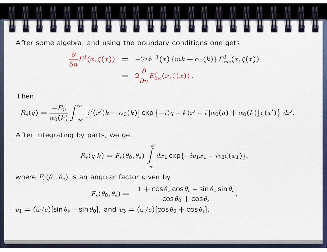
After some algebra, and using the boundary conditions one gets
∂
∂nEI(x, ζ(x)) = −2iφ−1(x) {mk+ α0(k)}EI
inc(x, ζ(x))
= 2∂
∂nEIinc(x, ζ(x)) .
Then,
Rs(q) =−E0
α0(k)
∫ ∞
−∞
[ζ ′(x′)k+ α0(k)
]exp
{−i(q − k)x′ − i [α0(q) + α0(k)] ζ(x
′)}dx′.
After integrating by parts, we get
Rs(q|k) = Fs(θ0, θs)
∞∫−∞
dx1 exp{−iv1x1 − iv3ζ(x1)},
where Fs(θ0, θs) is an angular factor given by
Fs(θ0, θs) = −1 + cos θ0 cos θs − sin θ0 sin θs
cos θ0 + cos θs,
v1 = (ω/c)[sin θs − sin θ0], and v3 = (ω/c)[cos θ0 + cos θs].

.
Summarizing, for a more general polarization case and a perfectly conducting surface,
the Kirchhoff source function is given by
FK(x1) =
{2ψinc (x1, ζ(x1)) in p polarization2(∂/∂N)ψinc (x1, ζ(x1)) in s polarization
.
Substitution into the scattering amplitude and integration by parts gives (Ogilvy, 1991)
Rp,s(q|k) = Fp,s(θ0, θs)
∞∫−∞
dx1 exp{−iv1x1 − iv3ζ(x1)},
where Fp,s(θ0, θs) is an angular factor given by
Fp,s(θ0, θs) = ±1 + cos θ0 cos θs − sin θ0 sin θs
cos θ0 + cos θs,
The “+” sign is for p polarization, and the “−” sign for s polarization.
The term v3ζ(x1) may be interpreted as the phase acquired by the wave upon reflection
from the surface.
For small angles of incidence and scattering, |Fp,s(θ0, θs)| ≈ 1 and v3 is practically
independent of θ0 and θs.

The thin phase screen model.
Thin-phase screen - layer of negligible thickness that introduces upon reflection (trans-
mission) phase variations in the reflected (transmitted) wave, without introducing any
amplitude variations (Ratcliffe, 1956, Welford, 1977).
θ0θs
scatterer ζscatterer
θ0θs
(a) (b)
Change in the optical path length:
φb − φa =(ωc
)(cos θ0 + cos θs)ζ.

For a surface with random height variations ζ(x1) the random phase coincides with
the result obtained with the Kirchhoff approximation.
In the thin phase screen approximation, the scattering amplitude is given by
R(q|k) = A0
∞∫−∞
dx1e−iv1x1−iv3ζ(x1),
where A0 = ψ0κ0, ψ0 is the amplitude of the incident plane wave, κ0 being a constant
that accounts for the average reflectance or transmittance of the sample, and
v1 = (ω/c)[sin θs − sin θ0],
v3 = (ω/c)[cos θ0 + cos θs].
Lateral features larger than the wavelength, small slopes, no multiple scattering.

.
Perturbation theory (small heights)
Einc(x, ζ(x)) + Esc(x, ζ(x)) = 0,
Using the Rayleigh hypothesis
E0 exp {ikx} exp {−iα0(k)ζ(x)} = −∫ ∞
−∞
dq
2πRs(q) exp {iqx} exp {iα0(q)ζ(x)} .
We multiply these equations by exp{−ipx}, and integrate with respect to x
E0
∫ ∞
−∞dx exp {i(k − p)x− iα0(k)ζ(x)} = −
∫ ∞
−∞dx
∫ ∞
−∞
dq
2πRs(q) exp {i(q − p)x+ iα0(q)ζ(x)} .
Defining
I(γ|Q) =
∫ ∞
−∞dxe−iQxe−iγζ(x),
we get
E0I(α0(k)|p− k) = −∫ ∞
−∞
dq
2πRs(q)I(−α0(q)|p− q).
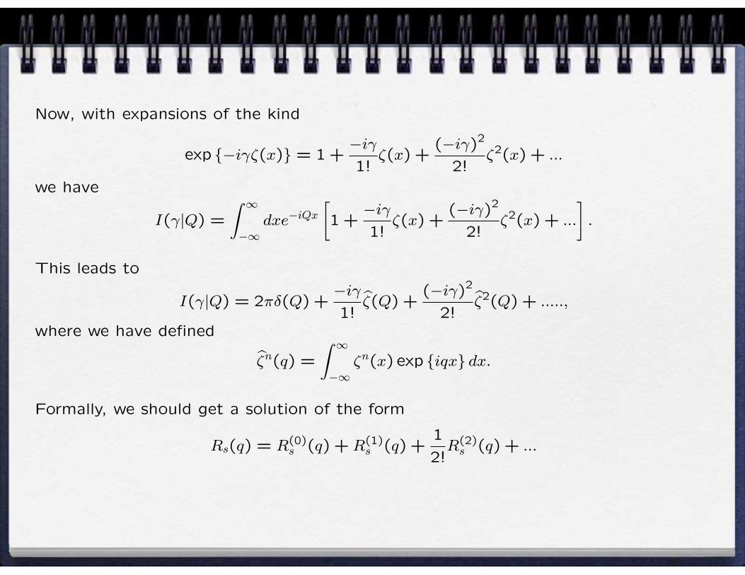
Now, with expansions of the kind
exp {−iγζ(x)} = 1 +−iγ1!
ζ(x) +(−iγ)2
2!ζ2(x) + ...
we have
I(γ|Q) =
∫ ∞
−∞dxe−iQx
[1 +
−iγ1!
ζ(x) +(−iγ)2
2!ζ2(x) + ...
].
This leads to
I(γ|Q) = 2πδ(Q) +−iγ1!
ζ(Q) +(−iγ)2
2!ζ2(Q) + .....,
where we have defined
ζn(q) =
∫ ∞
−∞ζn(x) exp {iqx} dx.
Formally, we should get a solution of the form
Rs(q) = R(0)s (q) +R(1)
s (q) +1
2!R(2)s (q) + ...

Coming back to our equation
E0
[2πδ(p− k) +
−iα0(k)
1!ζ(p− k) + ...
]= −
∫ ∞
−∞
dq
2π
[R(0)s (q) +R(1)
s (q)]×
×[2πδ(p− q) +
iα0(q)
1!ζ(p− q) + ...
].
Equating terms of equal order we find integral equations of the kind
E02πδ(p− k) = −∫ ∞
−∞
dq
2πR(0)s (q)2πδ(p− k),
E0−iα0(k)
1!ζ(p− k) = −R(1)
s (p)−∫ ∞
−∞
dq
2πR(0)s (q)
iα0(q)
1!ζ(p− q),
Solving these equations we finally get
Rs(p) = −2πδ(p− k)E0 + 2iα0(k)E0ζ(p− k) + ....
For a perfect conductor one can go up to high orders in s polarization, but in p
polarization the solution diverges for the order ζ2(p).
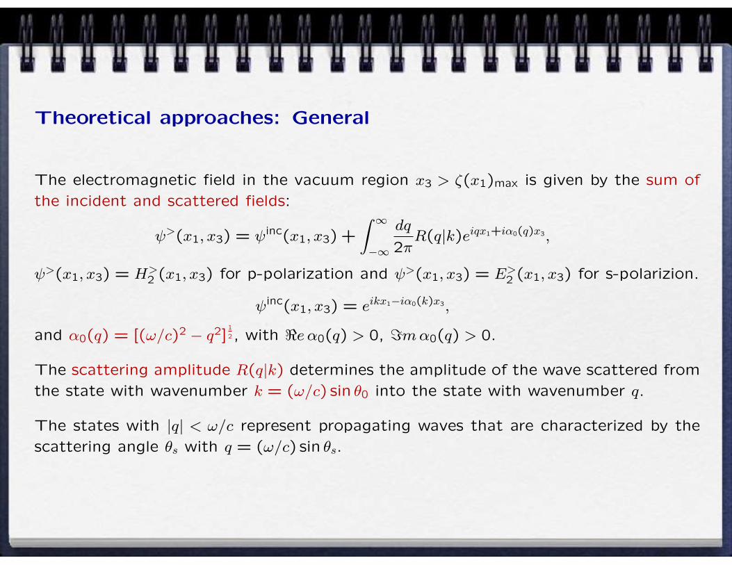
Theoretical approaches: General
The electromagnetic field in the vacuum region x3 > ζ(x1)max is given by the sum of
the incident and scattered fields:
ψ>(x1, x3) = ψinc(x1, x3) +
∫ ∞
−∞
dq
2πR(q|k)eiqx1+iα0(q)x3,
ψ>(x1, x3) = H>2 (x1, x3) for p-polarization and ψ>(x1, x3) = E>
2 (x1, x3) for s-polarizion.
ψinc(x1, x3) = eikx1−iα0(k)x3,
and α0(q) = [(ω/c)2 − q2]1
2, with <e α0(q) > 0, =mα0(q) > 0.
The scattering amplitude R(q|k) determines the amplitude of the wave scattered from
the state with wavenumber k = (ω/c) sin θ0 into the state with wavenumber q.
The states with |q| < ω/c represent propagating waves that are characterized by the
scattering angle θs with q = (ω/c) sin θs.

Theoretical approaches: The DRC and its averages
The differential reflection coefficient (DRC) - defined as the fraction of the total flux
incident onto the surface that is scattered into the angular interval dθs about the
scattering direction defined by the angle θs.
It is given by (∂R
∂θs
)=
1
2πL1
cos2 θscos θ0
|R(q|k)|2,
where L1 denotes the length of the x1-axis covered by the surface.
The calculation of R(q|k) is the central problem of rough surface scattering theory.
The mean differential reflection coefficient 〈∂R/∂θs〉 is given by⟨∂R
∂θs
⟩=
1
2πL1
ω
c
cos2 θscos θ0
〈|R(q|k)|2〉,
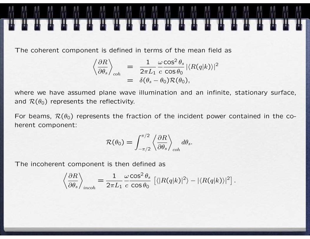
The coherent component is defined in terms of the mean field as⟨∂R
∂θs
⟩coh
=1
2πL1
ω
c
cos2 θscos θ0
|〈R(q|k)〉|2
= δ(θs − θ0)R(θ0),
where we have assumed plane wave illumination and an infinite, stationary surface,
and R(θ0) represents the reflectivity.
For beams, R(θ0) represents the fraction of the incident power contained in the co-
herent component:
R(θ0) =
∫ π/2
−π/2
⟨∂R
∂θs
⟩coh
dθs.
The incoherent component is then defined as⟨∂R
∂θs
⟩incoh
=1
2πL1
ω
c
cos2 θscos θ0
[〈|R(q|k)|2〉 − |〈R(q|k)〉|2
].

Rayleigh method
The y-component of the reflected and transmitted fields can be written as
ψR(x, z) =
∫ ∞
−∞
dq
2πR(q|k) exp[iqx+ iαI(q)z], z ≥ ζ(x),
ψT(x, z) =
∫ ∞
−∞
dq
2πT (q|k) exp[iqx− iαII(q)z], z ≤ ζ(x),
The continuity of the parallel components of E and H across the interface implies that
ψI(x, ζ(x)) = ψII(x, ζ(x)) ,
1
νI
∂
∂nψI(x, z)
∣∣∣∣z=ζ(x)
=1
νII
∂
∂nψII(x, z)
∣∣∣∣z=ζ(x)
,
where νR = 1 for s polarization and εR(ω) for p polarization.
Rayleigh hypothesis: The plane wave expansions for the fields in the regions x3 >
ζ(x1)max and x3 < ζ(x1)min can be continued onto the surface itself (Rayleigh, 1907).
.
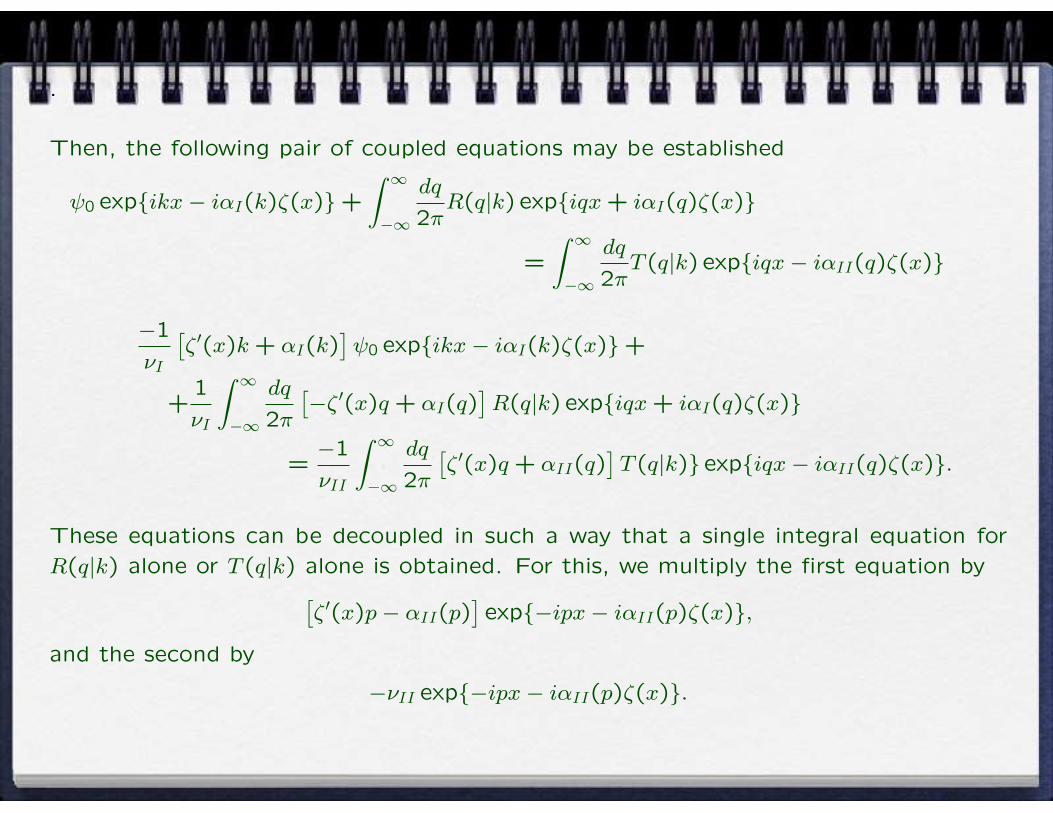
Then, the following pair of coupled equations may be established
ψ0 exp{ikx− iαI(k)ζ(x)}+
∫ ∞
−∞
dq
2πR(q|k) exp{iqx+ iαI(q)ζ(x)}
=
∫ ∞
−∞
dq
2πT (q|k) exp{iqx− iαII(q)ζ(x)}
−1
νI
[ζ ′(x)k+ αI(k)
]ψ0 exp{ikx− iαI(k)ζ(x)}+
+1
νI
∫ ∞
−∞
dq
2π
[−ζ ′(x)q+ αI(q)
]R(q|k) exp{iqx+ iαI(q)ζ(x)}
=−1
νII
∫ ∞
−∞
dq
2π
[ζ ′(x)q+ αII(q)
]T (q|k)} exp{iqx− iαII(q)ζ(x)}.
These equations can be decoupled in such a way that a single integral equation for
R(q|k) alone or T (q|k) alone is obtained. For this, we multiply the first equation by[ζ ′(x)p− αII(p)
]exp{−ipx− iαII(p)ζ(x)},
and the second by
−νII exp{−ipx− iαII(p)ζ(x)}.
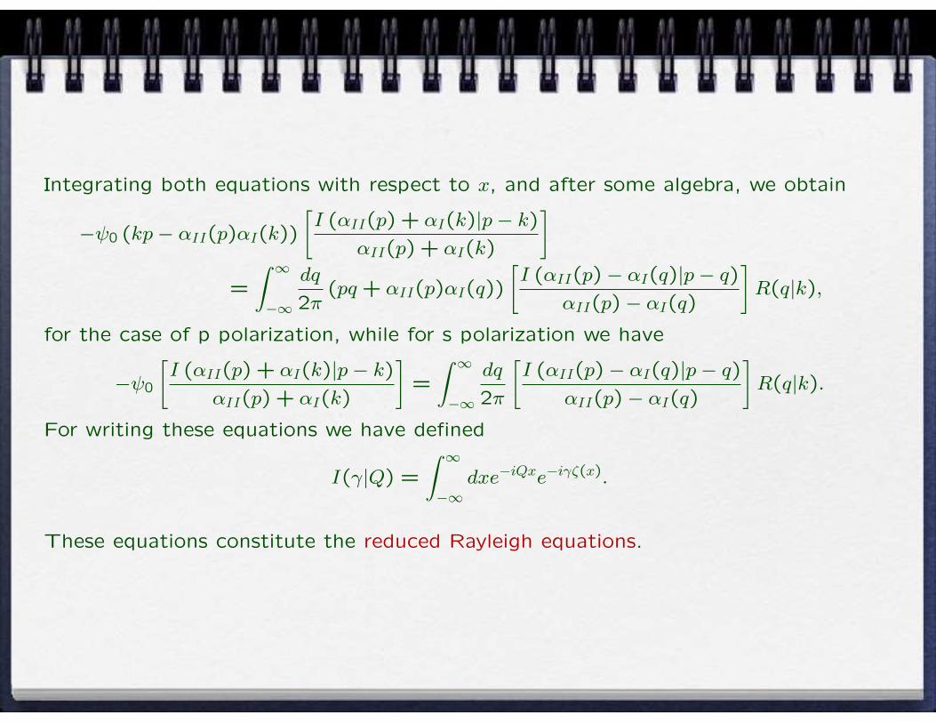
Integrating both equations with respect to x, and after some algebra, we obtain
−ψ0 (kp− αII(p)αI(k))
[I (αII(p) + αI(k)|p− k)
αII(p) + αI(k)
]=
∫ ∞
−∞
dq
2π(pq+ αII(p)αI(q))
[I (αII(p)− αI(q)|p− q)
αII(p)− αI(q)
]R(q|k),
for the case of p polarization, while for s polarization we have
−ψ0
[I (αII(p) + αI(k)|p− k)
αII(p) + αI(k)
]=
∫ ∞
−∞
dq
2π
[I (αII(p)− αI(q)|p− q)
αII(p)− αI(q)
]R(q|k).
For writing these equations we have defined
I(γ|Q) =
∫ ∞
−∞dxe−iQxe−iγζ(x).
These equations constitute the reduced Rayleigh equations.

Rayleigh method: Summary
Rayleigh hypothesis: The plane wave expansions for the fields in the regions x3 >
ζ(x1)max and x3 < ζ(x1)min can be continued onto the surface itself (Rayleigh, 1907).
These can be used in satisfying the boundary conditions at x3 = ζ(x1) to derive a
single integral equation for the scattering amplitude:∫ ∞
−∞
dq
2πM (+)(p|q)R(q|k) = −M (−)(p|k),
where
M (±)(p|q) =[pq ± α(p)α0(q)]µ
α(p)∓ α0(q)I[α(p)∓ α0(q)|p− q],
I[γ|Q] =
∫ ∞
−∞dx1e
−iQx1e−iγζ(x1),
and α(q) = [ε(ω)(ω/c)2 − q2]1/2.
The exponent µ is unity for p polarization and zero for s polarization.
Reduced Rayleigh equation - exact within the Rayleigh hypothesis.
The reduced Rayleigh equations (Toigo et al., 1977, Brown et al., 1983) constitute a
convenient starting point for the derivation of the perturbation theories
In perturbation theory, some function entering the expression for the intensity of the
scattered light is expanded in powers of the surface profile function.
It can be:
- the scattering amplitude (Rayleigh, 1896, Rayleigh, 1907, Rice, 1951),
- the phase of the scattering amplitude (Shen and Maradudin, 1980),
- or some other quantity (Maradudin, Luna and Mendez, 1983).
Also used for numerical Monte Carlo-type simulations:
- Generate a realization of the surface and solve.
- Repeat the procedure and average over many independent realization of the profile.

Integral equation method
Approach is based on the exact equations for electromagnetic fields derived with the
use of Green’s second integral theorem in the half-spaces x3 > ζ(x1) and x3 < ζ(x1).
The scattering amplitude R(q|k) is expressed in terms of the surface values of:
- the total field ψ(x1) ≡ ψ>(x1, ζ(x1)), and
- its unnormalized normal derivative υ(x1) = (∂/∂N) ψ>(x1, x3)∣∣x3=ζ(x1)
R(q|k) =i
2α0(q)
∫ ∞
−∞dx1
{i[qζ ′(x1)− α0(q)]ψ(x1)− υ(x1)
}e−iqx1−iα0(q)ζ(x1),
with ∂/∂N = −ζ ′(x1)(∂/∂x1) + (∂/∂x3).

The source functions ψ(x1) and υ(x1) obey a pair of coupled integral equations
ψ(x1) = ψinc(x1) +
∫ ∞
−∞dx′1 [H0(x1|x′1)ψ(x′1)− L0(x1|x′1)υ(x′1)],
0 =
∫ ∞
−∞dx′1 [Hε(x1|x′1)ψ(x′1)− νLε(x1|x′1)υ(x′1)],
where
Hε(x1|x′1) =i
4
∂
∂N ′H(1)0 [nc(ω/c)ξ]
∣∣x′3=ζ(x′1)
,
Lε(x1|x′1) =i
4H(1)
0 [nc(ω/c)ξ]∣∣x′3=ζ(x′1)
,
H(1)0 (z) is the Hankel function of the first kind, ξ =
[(x1 − x′1)
2 + (ζ(x1)− x′3 + η)2]1/2
,
η is a positive infinitesimal, and ν equals ε(ω) for p polarization and 1 for s polarization.
The kernels H0(x1|x′1) and L0(x1|x′1) are obtained by setting nc = 1 in Hε(x1|x′1) and
Lε(x1|x′1), respectively.
For a given surface and conditions of illumination, these equations can be solved
numerically to determine the source functions and, in turn, the scattering amplitude.
=> Monte Carlo simulation.
With two-dimensional surfaces x3 = ζ(x‖) the number of unknowns increases.
- more surface points.
- full vectorial nature of the field (more integral equations).
The case is often approached in the context of Dirichlet or Neumann surfaces and/or
a scalar model (Tran and Maradudin, 1992, Macaskill and Kachoyan 1993, Tran and
Maradudin, 1993).
Perfectly conducting surfaces (Tran, Celli and Maradudin, 1994).
Metallic surfaces (Tran and Maradudin, 1994).

The coherent component (TPS model)
The average scattering amplitude can be written as
〈R(q|k)〉 = A0
∞∫−∞
dx1e−iv1x1〈e−iv3ζ(x1)〉.
For the case of Gaussian phase fluctuations
〈e−iv3ζ(x1)〉 = e−v23δ
2/2.
Normalizing the reflectivity of the rough sample by the reflectivity of a flat surface we
obtain the resultR(θ0)
RF(θ0)= exp
{−v2
3δ2}.
Useful for estimating δ (but independent of the lateral scale!).
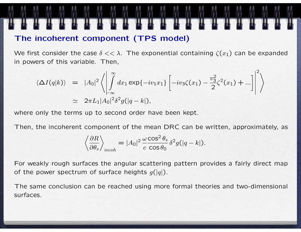
The incoherent component (TPS model)
We first consider the case δ << λ. The exponential containing ζ(x1) can be expanded
in powers of this variable. Then,
〈∆I(q|k)〉 = |A0|2⟨∣∣∣∣∣∣
∞∫−∞
dx1 exp{−iv1x1}[−iv3ζ(x1)−
v23
2ζ2(x1) + ...
]∣∣∣∣∣∣2⟩
' 2πL1|A0|2δ2g(|q − k|),
where only the terms up to second order have been kept.
Then, the incoherent component of the mean DRC can be written, approximately, as⟨∂R
∂θs
⟩incoh
= |A0|2ω
c
cos2 θscos θ0
δ2g(|q − k|).
For weakly rough surfaces the angular scattering pattern provides a fairly direct map
of the power spectrum of surface heights g(|q|).
The same conclusion can be reached using more formal theories and two-dimensional
surfaces.

The incoherent component (TPS model)
(b)(a)
0
0.2
0.4
0.6
0.8
1
-90 -60 -30 0 30 60 90
<∂R
s(θ s
)/∂
θ s>
inco
h
θs [deg]
0
0.1
0.2
0.3
0.4
-90 -60 -30 0 30 60 90
<∂R
s(θ s
)/∂
θ s>
inco
h
θs [deg]
The incoherent part of the differential reflection coefficient for (a) a surface with a
triangular power spectrum, and (b) a surface with a rectangular power spectrum.
The curves represent averages over 200 realizations of the random surfaces.

The incoherent component (TPS model)
Consider now the case δ >> λ. The mean intensity
〈I(q|k)〉 = |A0|2∞∫
−∞
dx1
∞∫−∞
dx′1e−iv1(x1−x′1)〈e−iv3[ζ(x1)−ζ(x′1)]〉.
With the change of variables x′1 = x1 + u, we can write
〈I(q|k)〉 = |A0|2L1
∞∫−∞
du e−iv1u g(u),
where g(u) = 〈e−iv3[ζ(x1)−ζ(x1+u)]〉. Since (ω/c)δ >> 1,
g(u) = 〈e−iv3uζ ′(x1)〉,
which is obtained by expressing the difference ζ(x1) − ζ(x1 + u) in powers of u. This
approximation leads to the result
〈I(q|k)〉 = |A0|22πL1
v3Pζ ′
(v1
v3
),
where Pζ ′(x) represents the PDF of slopes on the surface.

Comments:
Scattering Angle [deg]
-60 -30 0 30 60
<∂R
s(θ s
)/∂θ
s>
0
4
8
Scattering Angle [deg]
-90 -60 -30 0 30 60 90
<∂R
s(θ s
)/∂θ
s>
0
2
Weakly rough surfaces:
- δ can be estimated from the coherent component.
Rough surfaces:
- Speckle contains no information (universal law).
- The mean intensity is related to the PDF of slopes.
When changing the angle of incidence or the wavelength, the speckle correlation
contains information on δ.

Example: Corrections for the reflectivity.
The phase perturbation theory yields
Rp(θ0) =
∣∣∣∣∣ ε(ω) cos θ0 − (ε(ω)− sin2 θ0)1
2
ε(ω) cos θ0 + (ε(ω)− sin2 θ0)1
2
∣∣∣∣∣2
× exp
{−4
δ2
a2<e
[ε(ω)
ε(ω)− 1
cos θ0
ε(ω) cos2 θ0 − sin2 θ0
× µp
(θ0,
ωa
c
)]},
Rs(θ0) =
∣∣∣∣∣cos θ0 − (ε(ω)− sin2 θ0)1
2
cos θ0 + (ε(ω)− sin2 θ0)1
2
∣∣∣∣∣2
× exp
{−4
δ2
a2<e
cos θ01− ε(ω)
µs
(θ0,
ωa
c
)},
where µp,s(θ0, (ωa/c)) are defined by
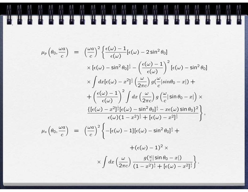
.
µp
(θ0,
ωa
c
)=
(ωac
)2{ε(ω)− 1
ε(ω)[ε(ω)− 2 sin2 θ0]
× [ε(ω)− sin2 θ0]1
2 −(ε(ω)− 1
ε(ω)
)2
[ε(ω)− sin2 θ0]
×∫dx[ε(ω)− x2]
1
2
( ω
2πc
)g(ω
c|sinθ0 − x|) +
+
(ε(ω)− 1
ε(ω)
)2 ∫dx
( ω
2πc
)g
(ωc| sin θ0 − x|
)×
{[ε(ω)− x2]1
2[ε(ω)− sin2 θ0]1
2 − xε(ω) sin θ0}2
ε(ω)(1− x2)1
2 + [ε(ω)− x2]1
2
},
µs
(θ0,
ωa
c
)=
(ωac
)2{−[ε(ω)− 1][ε(ω)− sin2 θ0]
1
2 +
+(ε(ω)− 1)2 ×
×∫dx
( ω
2πc
) g(ωc| sin θ0 − x|)
(1− x2)1
2 + [ε(ω)− x2]1
2
}.

θο[deg]0 30 60 90
Reflectivity
0.0
0.2
0.4
0.6
0.8
1.0
PPTSEPTSAPT
KA
(a)
CS
EXPT
θο[deg]0 30 60 90
Reflectivity
0.0
0.2
0.4
0.6
0.8
1.0
PPTSEPTSAPT
KA
(b)
CS
EXPT
Reflectivity as a function of the angle of incidence. λ = 5.5µm. Gold surface with
δ = 0.38µm, a = 2.8µm. (a) p-polarization; (b) s-polarization.

Example: Knotts, Michel, and O’Donnell, JOSAA 10, 928 (1993).


Example: Plasmons and multiple scattering
Fourth-order perturbation theory (Maradudin and Mendez, 1993).
〈∂Rp
∂θs〉incoh =
1
L1
2
π
(ωc
)3cos2 θs cos θ0|G0(q)|2{
〈|T (1)(q|k)|2〉+1
4
[〈|T (2)(q|k)|2〉 − |〈T (2)(q|k)〉|2
]−
1
3<e〈T (1)(q|k)∗T (3)(q|k)〉
}|G0(k)|2
with
G0(k) =iε(ω)
ε(ω)α0(k) + α(k).
The expression has the form
〈∂Rp
∂θs〉incoh = (1− 1) + (2− 2) + (1− 3)

.
Scattering Angle [deg]
-90 -60 -30 0 30 60 90
<∂ R
p/∂θ
s>
0.000
0.002
0.004
0.006
0.008
0.010
0.012
total
(1-1)
(2-2)
-(1-3)
δ=5 nm
a=100 nm
λ=457.9 nmsilver surface
Surface plasmons and multiple scattering

West-O’Donnell power spectrum
k
kspk- sp
G(k)−ω /c ω /cω

.
Gold surface in p polarization. δ = 10.9nm, θmax = 13.45◦, λ = 612nm.
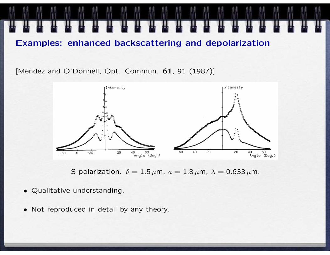
Examples: enhanced backscattering and depolarization
[Mendez and O’Donnell, Opt. Commun. 61, 91 (1987)]
S polarization. δ = 1.5µm, a = 1.8µm, λ = 0.633µm.
• Qualitative understanding.
• Not reproduced in detail by any theory.

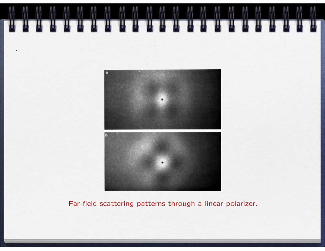
.
Far-field scattering patterns through a linear polarizer.

Some challenges
Ocean-like surfaces
Low frequency (gravity waves, etc.): S1(k) - Pierson-Moskowitz (1964) spectrum
S1(|k|) =a0
2|k|3exp
{−
0.74g2
|k|2u410
},
where a0 = 1.4 × 10⁻³, g = 9.81m/s2 is the gravity constant, and u10 is the wind
velocity at 10 meters above the mean sea level.
High frequency (capillary waves, etc.): S2(|k|) - Pierson and Stacy (1974).
S2(|k|) = 0.4375(2π)p−1(1 + 3k2/k2
m
)g(1−p)/2
(|k|+ |k|3/k2
m
)−(1+p)/2.
where p = 5 − log10(u∗), u∗ is the wind friction velocity in cm/s, k2m = gρ/τ , ρ is the
water density, and τ represents the surface tension for sea water. A typical value for
km is 3.62 rad/cm (Fung and Lee, 1982).

.
k [1/cm]
0.001 0.01 0.1 1 10
S(k
[cm
3 ]
1e-5
1e-4
1e-3
1e-2
1e-1
1e+0
1e+1
1e+2
1e+3
1e+4
1e+5
k max
/819
2
ω/c kmax
k max
/409
6
k max
/204
8
k max
/512
k max
/102
4
k=0.04
Full spectrum of the surface. S1(k) and S2(k) have been matched at k = 0.04. The
sampling is ∆x = λ/10 (kmax = 10ω/c). We show lines at kmin = kmax/N , where N is
the number of points on the surface.

Hei
ght [
cm]
-10
0
10
Hei
ght [
cm]
-10
0
10
Hei
ght [
cm]
-10
0
10
Hei
ght [
cm]
-10
0
10
Position [cm]
-2000 -1500 -1000 -500 0 500 1000 1500 2000
Hei
ght [
cm]
-10
0
10
kmin=kmax / 2048
kmin=kmax / 512
kmin=kmax / 1024
kmin=kmax / 8192
kmin=kmax /
4096

Some challenges
• Statistical modeling
• Large systems
• Grazing angles of incidence
• Surface and bulk
• 2D surfaces
• Characterization of surfaces
• Fabrication of surfaces

Inverse Scattering with Amplitude Data
x1
x3
3 1ζx = (x )
inck
sθ
Es Ep
sck
k
oθEp
Esq
α (q)oα (k)o
Objective: Determine the profile from scattering data.

Plane wave illumination.
The incident field is given by
ψ(pw)2 (x1, x3)inc = ψ0 exp {ikx1 − iα0(k)x3} ,
where
k =ω
csin θ0 , α0(k) =
ω
ccos θ0 .
The field scattered by the surface is
ψ(pw)2 (x1, x3)sc =
∞∫−∞
dq
2πRp,s(q|k) exp {iqx1 + iα0(q)x3} ,
where
α0(q) =
√(ωc
)2− q2 .
For propagating waves,
q =ω
csin θs , α0(q) =
ω
ccos θs

Focussed beam
Consider the case in which the surface is illuminated with a superposition of plane
waves
ψ2 (x1, x3; ξ, η)inc =
∞∫−∞
dk
2πP (k) exp {ik (x1 − ξ)− iα0(k) (x3 − η)} .
For the case in which P (k) is constant, this field represents a converging beam, and
(ξ, η) is the point of convergence.
Due to the linearity of the problem, the scattered field can be written as a superposition
of plane wave solutions. We find
ψ2 (x1, x3; ξ, η)sc =
∞∫−∞
dk
2π
∞∫−∞
dq
2πP (k)Rp,s(q|k)×
× exp {iqx1 − ikξ+ iα0(q)x3 + iα0(k)η} .

The wavefront matching algorithm
x1
3x
x1
3x

The wavefront matching algorithm
Let us consider the function
V (ξ, η) =
∫ ∞
−∞|ψ2 (x1, x3; ξ, η)sc + ψ∗2 (x1, x3; ξ, η)inc|
2 dx1
= 2K +
∫ ∞
−∞[ψ2 (x1, x3; ξ, η)scψ2 (x1, x3; ξ, η)inc + c.c.] dx1,
where is a K is a constant that represents the total incident intensity.
Let us consider the function U , related to the interference term
U (ξ, η) =
∫ ∞
−∞ψ2 (x1, x3; ξ, η)scψ2 (x1, x3; ξ, η)inc dx1.
It is expected that U (ξ, η) is maximized (or minimized) when (ξ, η) = (x1, ζ(x1)).
Fwm(ξ, η) = 2<e{U(ξ, η)} Fconf(ξ, η) = |U(ξ, η)|2
“Interferometric Confocal” “Confocal”

After some algebra
U (ξ, η) =
∞∫−∞
dk
2π
∞∫−∞
dq
2πP (k)P (−q)Rp,s(q|k)Φ(q, k|ξ, η),
where P (k) is a pupil function, and
Φ(q, k|ξ, η) = exp {−i (k − q) ξ+ i (α0(k) + α0(q)) η} .
The function U (ξ, η) forms the basis of our algorithm.
We assume that we have scattering data corresponding to several angles of incidence.
That is, we have Rp,s(q|k) as a function of k and q (θ0 and θs).

The direct problem
-1.5
-1
-0.5
0
0.5
1
1.5
2
-14 -12 -10 -8 -6 -4 -2 0 2 4 6 8 10 12 14
Hei
ght [
wav
elen
gths
]
x [wavelengths]
k
q
-5 0 5-6
-4
-2
0
2
4
6
1.5
1
0.5
0
0.5
1
1.5
k
q
-5 0 5-6
-4
-2
0
2
4
6
(a) Amplitude (b) Phase
5
10
15
20
a=2λ δ=λ/2

Interferometric confocal
100
50
0
50
100
[wavelengths]
[w
avel
engt
hs]
(a) p polarization
-15 -10 -5 0 5 10 15-3
-2
-1
0
1
2
3
[wavelengths]
[w
avel
engt
hs]
(b) s polarization
-15 -10 -5 0 5 10 15-3
-2
-1
0
1
2
3
100
50
0
50
100

Confocal
0.5
1
1.5
2
x 104
0.5
1
1.5
2
x 104
(a) p polarization
(b) s polarization
[w
avel
engt
hs]
-3
-2
-1
0
1
2
3
[wav
elen
gths
]
-3
-2
-1
0
1
2
3
[wavelengths]-15 -10 -5 0 5 10 15
[wavelengths]-15 -10 -5 0 5 10 15

Air-Glass-Silver: Confocal
s polarization confocal
[wavelengths]
[wav
elen
gths
]
-15 -10 -5 0 5 10 15
-2
0
2
p polarization confocal
[wavelengths]
[wav
elen
gths
]
-15 -10 -5 0 5 10 15
-2
0
2

The point spread function
z [w
avel
engt
hs]
PSF through an interface at z=1
-10 -5 0 5 10
-4
-2
0
2
4
z [w
avel
engt
hs]
PSF in vacuum
-10 -5 0 5 10
-4
-2
0
2
4
z [w
avel
engt
hs]
PSF through an interface at z=2
-10 -5 0 5 10
-4
-2
0
2
4
x [wavelengths]
z [w
avel
engt
hs]
PSF through an interface at z=3
-10 -5 0 5 10
-4
-2
0
2
4
x [wavelengths]
z [w
avel
engt
hs]
PSF in vacuum
-10 -5 0 5 10
-4
-2
0
2
4
z [w
avel
engt
hs]
corrected PSF for z=1
-10 -5 0 5 10
-4
-2
0
2
4
x [wavelengths]
z [w
avel
engt
hs]
corrected PSF for z=3
-10 -5 0 5 10
-4
-2
0
2
4
z [w
avel
engt
hs]
corrected PSF for z=2
-10 -5 0 5 10
-4
-2
0
2
4
x [wavelengths]
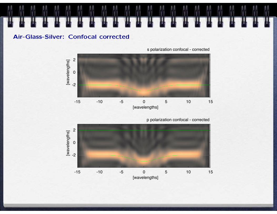
Air-Glass-Silver: Confocal corrected
s polarization confocal - corrected
[wavelengths]
[wav
elen
gths
]
-15 -10 -5 0 5 10 15
-2
0
2
p polarization confocal - corrected
[wavelengths]
[wav
elen
gths
]
-15 -10 -5 0 5 10 15
-2
0
2

Comments
• Variations of an algorithm for inverse scattering problems. The procedure can be
viewed as a synthetic confocal microscope.
• The procedure can be applied to metallic, dielectric and to layered structures.
With layered structures an adaptive pupil function must be used to correct for
spherical aberration.
• A sampling strategy for the scattering data (angles of incidence and scattering)
has been proposed.
• The algorithm is fairly robust and works well in regions where single scattering
is dominant. It is fairly insensitive to amplitude noise and tolerates some phase
noise.
• The method can be used with two-dimensional surfaces.

Inverse scattering with intensity data
We consider a perfectly conducting, one-dimensional, rough surface, illuminated with
an s-polarized plane wave:
E2 (x1, x3|ω)inc = ψ0 exp{ikx1 − iα0(k)x3}.
inck
sθ
Es Ep
sck
k
oθEp
Esq
x3
x1
x =ζ(x )13
• ζ(x1) represents the surface profile function.
• k = ωcsin θ0, and α0(k) =
√ω2/c2 − k2.

The scattered field can be written as
E2 (x1, x3|ω)sc =
∫ ∞
−∞
dq
2πRs(q|k) exp{iqx1 + iα0(q)x3},
with q = ωcsin θs, and α0(q) =
√ω2/c2 − q2,
Rs(q|k) =−i
2α0(k)
∞∫−∞
dx1
[exp{−iα0(q)ζ(x1)}F (x1|ω)
]exp{−iqx1},
and where
F (x1|ω) =
(−ζ ′(x1)
∂
∂x1+
∂
∂x3
)E2(x1, x3)|x3=ζ(x1).
The far-field intensity is given by
I(q|k)sc = |Rs(q|k)|2.
The objective:
to retrieve the surface profile function ζ(x1) from I(q|k)sc .
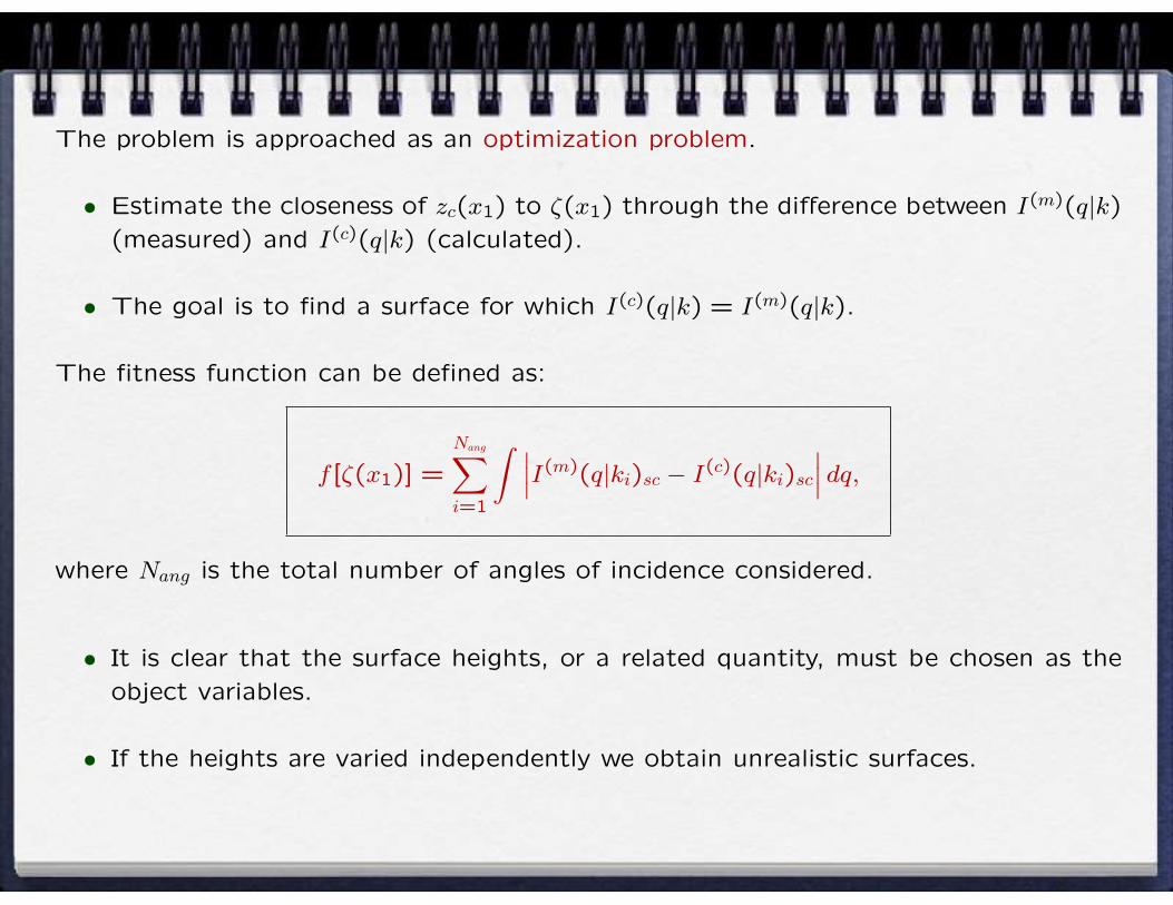
The problem is approached as an optimization problem.
• Estimate the closeness of zc(x1) to ζ(x1) through the difference between I(m)(q|k)(measured) and I(c)(q|k) (calculated).
• The goal is to find a surface for which I(c)(q|k) = I(m)(q|k).
The fitness function can be defined as:
f [ζ(x1)] =
Nang∑i=1
∫ ∣∣∣I(m)(q|ki)sc − I(c)(q|ki)sc∣∣∣ dq,
where Nang is the total number of angles of incidence considered.
• It is clear that the surface heights, or a related quantity, must be chosen as the
object variables.
• If the heights are varied independently we obtain unrealistic surfaces.

Representation of the surfaces by the spectral method
The surfaces are random and belong to a well-defined statistical class:
- GRP with a GCF.
Real array representing
the heights of the surface
M1 M2 M3 ... Mn/2 Mn/2+1 M ... M3 M2
N1 N2 N3 ... Nn/2 Nn/2+1 Nn/2 ... -N3 -N2
ζ 1 ζ2 ζ 3 ... ... ... ... ζ n-2 ζ -n 1 ζ n
Hermitian array { Mj + i Nj} /21/2
x
Root of powerspectrum
of surface [g(qj)]1/2
{ ζ n}
Fourier transform
-
n/2

Representation of the surfaces with spline curves
ζ(x1) =n∑
j=1
αjBkj (x1)
where Bkj (x1) is the jth B-spline function of order k, and the αj are the heights of the
control points.
-6 -4 -2 0 2 4 6-4
-3
-2
-1
0
1
2
3
x1 [wavelenghts]
Hei
ght [
wav
elen
ghts
]

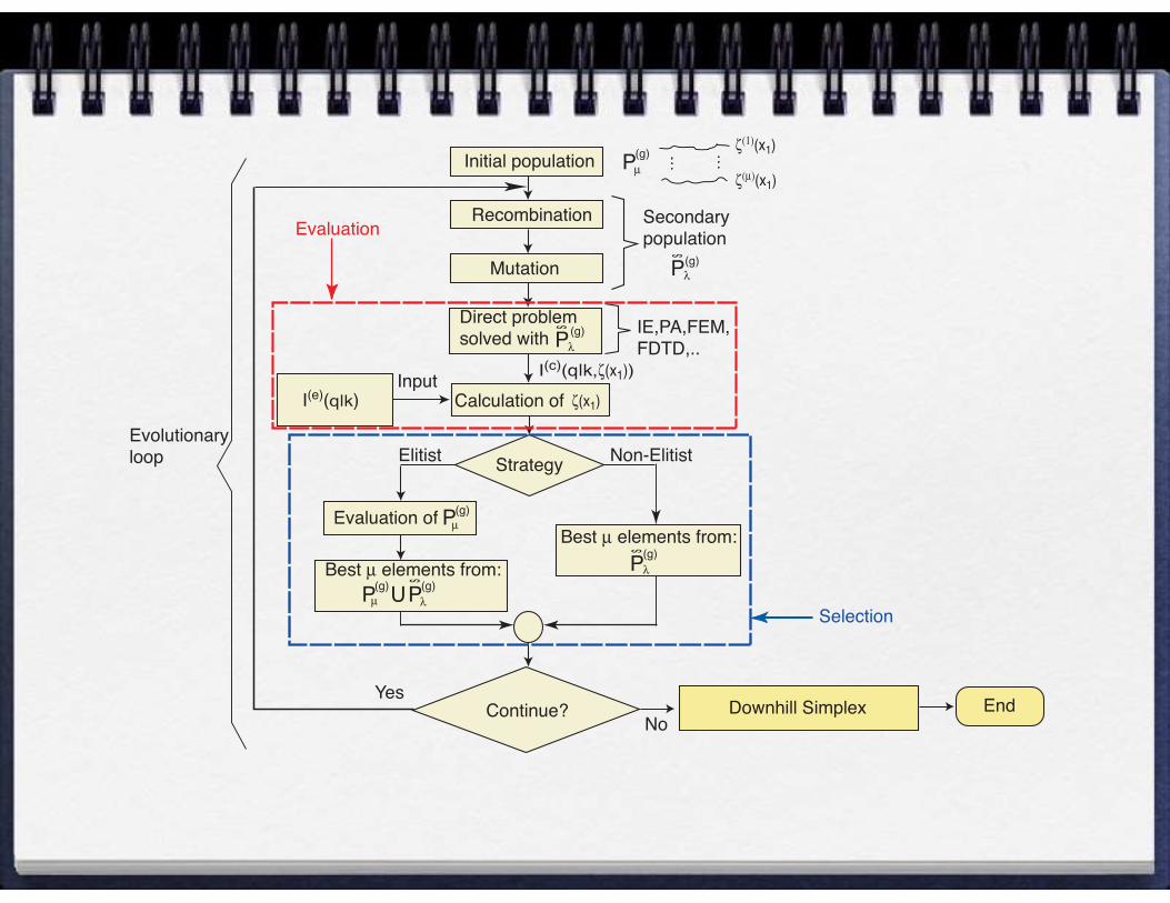
Evolutionary Strategies (ES)
The algorithm:
• Propose an initial population of µ (parent) surfaces.
• Combine and mutate them to produce a secondary population of λ (offspring)
new surfaces.
• Selection scheme:
– Elitist (µ/ρ + λ): retains the best µ surfaces from the evaluated initial and
secondary populations.
– Non-elitist (µ/ρ, λ): best µ surfaces from the evaluated secondary population.

Mutation
x
[g(qj)] 1/2
z1 z2 z3 ... ... ... ... zn-2 z -n 1 zn
Fourier transform
New array {Y j + i Z j}/21/2
Original random Hermitian array { Mj + i Nj } /21/2
M2 M 3 ... Mn/2 Mn/2+1 ... M3 M2
N1 N2 N3 ... Nn/2 Nn/2+1 ... -N3 -N2-Nn/2
Mn/2M1
M2 y3 ... yn/2 Mn/2+1 ... y3 M2
N1 N2 z3 ... zn/2 Nn/2+1 ... -z3 -N2-zn/2
yn/2M1
Surface heights {zn}
ζ(1)(x1)
Elitist Non-Elitist
Yes
NoContinue?
Evolutionaryloop
P(g)µInitial population
UP(g)µ
s
P(g)λ
Best µ elements from:
s
P(g)λ
Best µ elements from:
Mutation
Recombination
s
P(g)λ
Secondarypopulation
Strategy
Evaluation of P(g)µ
Direct problem solved with
s
P(g)λ
InputI(e)(q|k)
IE,PA,FEM,FDTD,..
I(c)(q|k,ζ(x1))
Calculation of ζ(x1)
Evaluation
Selection
EndDownhill Simplex
ζ(µ)(x1)

Numerical experiments
Spectral method:
• The profiles are realizations of a Gaussian random process with Gaussian corre-
lation function with a = 2λ and δ = λ/2.
Spline curve representation:
• The profiles were represented by spline curves. They can be random or determin-
istic.
Input data:
• Define a surface of length L (12.8 λ).
• Calculate I(q|k) for 4 angles of incidence (−60◦, −30◦, 0◦, and 40◦).
For the evolutionary loop the termination criterion was the maximum number of
iterations (g = 300 generations).

Reconstruction of random profiles
x 1 [wavelengths]
-6 -4 -2 0 2 4 6
Hei
ght
[wav
elen
gths
]
-1.0
-0.5
0.0
0.5
1.0
1.5
x 1 [wavelengths]
-6 -4 -2 0 2 4 6
(a) (b)
(a) Non-elitist (µ, λ) strategy. (b) Elitist (µ+ λ) strategy.

x 1 [wavelengths]
-6 -4 -2 0 2 4 6
Hei
ght
[wav
elen
gths
]
-1.0
-0.5
0.0
0.5
1.0
1.5
x 1 [wavelengths]
-6 -4 -2 0 2 4 6
(a) (b)
Two different initializations of the non-elitist (µ, λ) strategy.
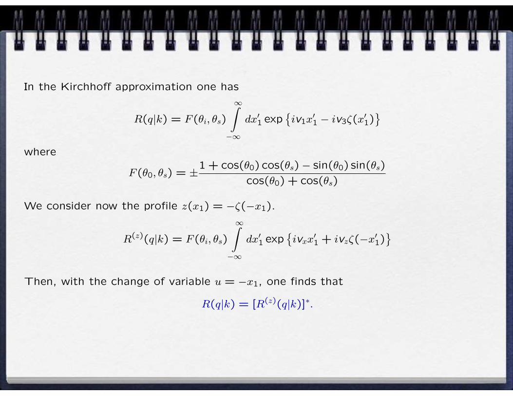
In the Kirchhoff approximation one has
R(q|k) = F (θi, θs)
∞∫−∞
dx′1 exp{iv1x
′1 − iv3ζ(x
′1)
}where
F (θ0, θs) = ±1 + cos(θ0) cos(θs)− sin(θ0) sin(θs)
cos(θ0) + cos(θs)
We consider now the profile z(x1) = −ζ(−x1).
R(z)(q|k) = F (θi, θs)
∞∫−∞
dx′1 exp{ivxx
′1 + ivzζ(−x′1)
}Then, with the change of variable u = −x1, one finds that
R(q|k) = [R(z)(q|k)]∗.

Comments
• The solution of the inverse scattering problem is not unique.
– Use several angles of incidence and polarizations. Multiple scattering (depar-
ture from Kirchhoff) also helps.
• The B-spline representation.
– Adequate for deterministic and random surfaces. Permits the use of recom-
bination in the main loop.
• In general, recombination helps to obtain convergence.
• The solution with the lowest fitness value was the right one.
• The use of ES + DH simplex leads to an additional improvement.