eu land markets - archive of european...
TRANSCRIPT
EU LAND MARKETS AND THE
COMMON AGRICULTURAL POLICY
PAVEL CIAIAN D’ARTIS KANCS
AND JOHAN F.M. SWINNEN
CENTRE FOR EUROPEAN POLICY STUDIES BRUSSELS

The Centre for European Policy Studies (CEPS) is an independent policy research institute based in Brussels. Its mission is to produce sound analytical research leading to constructive solutions to the challenges facing Europe today.
This publication is based on the Study on the Functioning of Land Markets in the EU Member States under the Influence of Measures applied under the Common Agricultural Policy, which was undertaken for the European Commission, Directorate-General for Agriculture and Rural Development (under contract 30-CE-0165424/00-86).
The opinions expressed in this publication and the analysis and arguments given are the sole responsibility of the authors writing in a personal capacity and do not necessarily reflect those of CEPS or any other institution with which the authors are associated.
Cover: Vincent van Gogh Wheat Fields after the Rain (the Plain of Auvers), 1890
Carnegie Museum of Art, Pittsburgh
ISBN 978-92-9079-963-4 © Copyright 2010, European Union and Centre for European Policy Studies
All rights reserved. No part of this publication may be reproduced, stored in a retrieval system or transmitted in any form or by any means – electronic, mechanical, photocopying, recording or otherwise – without the prior permission of the Centre for European Policy Studies and the European Union.
Centre for European Policy Studies Place du Congrès 1, B-1000 Brussels
Tel: 32 (0) 2 229.39.11 Fax: 32 (0) 2 219.41.51 e-mail: [email protected]
internet: http://www.ceps.eu

CONTENTS
Acknowledgements......................................................................................................i
List of abbreviations .................................................................................................. ii
Executive Summary................................................................................................... iii
1. Introduction......................................................................................................... 1
2. Conceptual framework...................................................................................... 3 2.1 The basic model........................................................................................ 3 2.2 Insights from empirical studies.............................................................. 5 2.3 Implementation of the SPS and implications ....................................... 7 2.4 Static versus dynamic effects.................................................................. 9 2.5 Empirical considerations for measuring the impact
of the SPS................................................................................................. 10 2.6 Summary: Key hypotheses on the effects of the SPS
on subsidy capitalisation into land values ......................................... 14
3. Data sources....................................................................................................... 18 3.1 Eurostat.................................................................................................... 18 3.2 Directorate-General for Agriculture and Rural
Development........................................................................................... 19 3.3 National statistics ................................................................................... 20 3.4 Farm Accountancy Data Network....................................................... 27 3.5 Interviews with local land-market experts......................................... 28
4. Socio-economic structure of the agricultural sector................................... 30 4.1 Unemployment and GDP ..................................................................... 30 4.2 Share of agriculture in employment and gross value added........... 30 4.3 Farm structure ........................................................................................ 31 4.4 Agricultural output and labour productivity .................................... 31 4.5 Output and input prices........................................................................ 32 4.6 Yields ....................................................................................................... 33 4.7 Agricultural income............................................................................... 33
5. Land sales markets in the EU......................................................................... 34 5.1 Sales market regulations ....................................................................... 34

5.2 Development of the land sales markets ..............................................50 5.3 Drivers of sales prices for agricultural land........................................72
6. Land rental markets in the EU........................................................................90 6.1 Rental market regulations .....................................................................90 6.2 Evolution of the rental market............................................................104 6.3 Drivers of rental prices ........................................................................117
7. Implementation of the SPS...........................................................................124 7.1 SPS implementation models ...............................................................125 7.2 Explaining the choice of SPS model...................................................125 7.3 Empirical evidence on the implementation of the SPS ...................128 7.4 The tradability of entitlements ...........................................................133 7.5 Cross-compliance .................................................................................135 7.6 National reserves ..................................................................................135
8. Impact of the SPS on land markets .............................................................137 8.1 Market for SPS entitlements................................................................137 8.2 Impact of the SPS on land markets ....................................................148 8.3 Effects of the SPS on structural change .............................................174 8.4 Influence of changes in the SPS models on land values..................179
9. General conclusions .......................................................................................182 9.1 Land markets in the EU study countries...........................................182 9.2 CAP reform and land markets............................................................184 9.3 Limitations.............................................................................................191
Bibliography .............................................................................................................193
Figures........................................................................................................................204
Tables .........................................................................................................................250
Appendix 1. Literature review...............................................................................283 Introduction.....................................................................................................283 Capitalisation of coupled subsidies .............................................................284 Capitalisation of decoupled subsidies .........................................................287 Determinants of subsidy capitalisation .......................................................288 Simulation studies ..........................................................................................295 Empirical studies on land (sales) prices ......................................................299

Empirical studies on land rents.................................................................... 304 Summary ......................................................................................................... 307
Appendix 2. Conceptual framework.................................................................... 310 Introduction .................................................................................................... 310 Static effects of the SPS .................................................................................. 311 Summary ......................................................................................................... 329
Appendix 3. Empirical approach .......................................................................... 330 Introduction .................................................................................................... 330 Estimating the impact of subsidies on land rents ...................................... 331 Estimating the impact of subsidies on land values/(sales) prices .......... 338 Summary ......................................................................................................... 341
Appendix 4. Determination of land value .......................................................... 342
List of Figures
Figure 1. Evolution of real sales prices for agricultural land in the EUSCs, 1992–2007 (€/ha) .........................................................204
Figure 2. Evolution of sales price indices for agricultural land in the EUSCs, 1992–2007 (%, 1992=100) ............................................204
Figure 3. Evolution of agricultural land sales as a percentage of total UAA in the EUSCs, 1992–2007..............................................205
Figure 4. Evolution of real rental prices for agricultural land in the EUSCs, 1992–2006 (€/ha) .........................................................205
Figure 5. Evolution of rental price indices for agricultural land in the EUSCs, 1992–2007 (€/ha) .........................................................206
Figure 6. Evolution of the rented share of the total agricultural area in the EUSCs, 1992–2006 (%) ..............................................................206
Figure 7. Development of unemployment rates ..............................................207
Figure 8. Real GDP per capita in purchasing power standards.....................207
Figure 9. Share of agriculture in total employment.........................................208
Figure 10. Share of gross value added of agriculture, fishing and hunting in total gross value added (%) .....................................208
Figure 11. Development of farm size in the EUSCs...........................................209

Figure 12. Development of real agricultural output in the EUSCs (1993=100)............................................................................................. 209
Figure 13. Development of real agricultural output in the EUSCs (in basic prices) .................................................................................... 210
Figure 14. Changes in agricultural labour productivity (output per AWU) in the EUSCs (1993=100) ................................... 210
Figure 15. Development of real input prices in key EU markets (index, 1993=100) ................................................................................. 211
Figure 16. Changes in agricultural output per AWU (% change in 2007 relative to 1993) ................................................... 211
Figure 17. Development of real crop prices in key EU markets (index, 1993=100) ................................................................................. 212
Figure 18. Development of real animal prices in key EU markets (index, 2000=100) ................................................................................. 212
Figure 19. Development of yields in the EUSCs (index, 1994=100) ................ 213
Figure 20. Relative yields by country (average 2005–06) ................................. 213
Figure 21. Index of the real income of agricultural factors per AWU ............ 214
Figure 22. Change in the real income of agricultural factors per AWU by country........................................................................... 214
Figure 23. Share of activated entitlements in the UAA (%) ............................. 215
Figure 24. Distribution of SPS entitlements in the Netherlands and Sweden .......................................................................................... 215
Figure 25. Value of SPS entitlements by region type in Italy, 2007................. 216
Figure 26. Impact of naked land on entitlement trading in the EUSCs.......... 216
Figure 27. Impact of restrictions on entitlement trading in the EUSCs.......... 217
Figure 28. Impact of naked land on entitlement market prices in the EUSCs......................................................................................... 217
Figure 29. Development of real land sales prices in Sweden (1990=100)....... 218
Figure 30. Development of real land rental prices in Germany (1997=100) .. 218
Figure 31. Land renting in the EU, 2005 (% of UAA)........................................ 219
Figure 32. Number of full- and part-time farms in Germany.......................... 219
Figure 33. Reported real rental prices of arable land and permanent grassland in Belgium........................................................................... 220

Figure 34. Regional differences in rental prices in Belgium, 2006 ...................220
Figure 35. Evolution of the deflated entrepreneurial income/AWU in Belgium .............................................................................................221
Figure 36. Evolution of the number of land sales in Belgium ..........................221
Figure 37. Average real prices of arable land and permanent grassland in Flanders and Wallonia: All plots...................................................222
Figure 38. Evolution of real input and output prices in Belgium....................222
Figure 39. Evolution of interest rates for land purchases in Belgium .............223
Figure 40. Nominal land prices, the number of transactions and transacted area in Finland, 1990–2007 .......................................223
Figure 41. Evolution of the total number of farmland sales transactions in France, 1994–2004 ............................................................................224
Figure 42. Evolution of the farmland sales area transacted in France, 1994–2004 ..............................................................................................224
Figure 43. Evolution of the average sales price of farmland in France, Bretagne and Centre regions, 1994–2004 ..........................................224
Figure 44. Evolution of several indicators in France (indices, 1994=100) .......225
Figure 45. Evolution of real farm income per worker (AWU) in France, 1990–2005 ..............................................................................................225
Figure 46. Share of rented land in Germany.......................................................226
Figure 47. Average land rents in Germany, 1991–2007.....................................226
Figure 48. Trends in land rents in Germany, 1991–2007 ...................................227
Figure 49. Land sales prices and the total number of sales transactions in Germany, 1991–2006 .......................................................................227
Figure 50. Indices of Irish agricultural land prices and rental rates (1997=100) .............................................................................................228
Figure 51. Trend in land prices in Italy (1990=100) ...........................................228
Figure 52. Land price developments for selected Dutch regions.....................229
Figure 53. Distribution of sales prices for arable land in the Netherlands.....229
Figure 54. Average transaction size per province in the Netherlands............230
Figure 55. Number of sales transactions and total area sold in the Netherlands................................................................................230
Figure 56. Rents for land in the Netherlands......................................................231

Figure 57. New rental contracts and total newly rented area in the Netherlands............................................................................... 231
Figure 58. Index for land prices and index for cereals in the Netherlands.... 232
Figure 59. Prices for agricultural land across Europe in 2006.......................... 232
Figure 60. Long-term interest rates in the Netherlands are falling, reducing the cost of financing for farms .......................................... 233
Figure 61. Share of agricultural land sales in the total utilised area in Sweden ............................................................................................. 233
Figure 62. Average plot size for transacted land in Sweden (hectares) ......... 234
Figure 63. Development of land sales prices in Sweden (1990=100) .............. 234
Figure 64. Annual changes in land prices in Sweden ....................................... 235
Figure 65. Regional differences in land sales prices in Sweden (€1,000/ha)............................................................................................ 235
Figure 66. Evolution of agricultural land rental rates in Sweden (1994=100)............................................................................................. 236
Figure 67. Impacts of the various drivers on Swedish agricultural land prices during 2003–07, average from the survey.................... 236
Figure 68. Impacts of the various drivers on Swedish agricultural land rents during 2003–07, average from the survey ..................... 237
Figure 69. Repo rate of interest* and land prices in Sweden ........................... 237
Figure 70. Average of all types of farmland values in the UK......................... 238
Figure 71. Average area of publicly marketed land and value in the UK ..... 238
Figure 72. Average English land values and publicly marketed land for sale ................................................................................................... 239
Figure 73. English land tenures............................................................................ 239
Figure 74. Land tenures in Northern Ireland..................................................... 240
Figure 75. Average area of land sold and values in Northern Ireland........... 240
Figure 76. Scottish land tenures ........................................................................... 241
Figure 77. Average Scottish land values and publicly marketed land for sale ................................................................................................... 241
Figure 78. Effect of the regional SPS model on the land market ..................... 242
Figure 79. Effect of the historical SPS model on the land market ................... 243

Figure 80. Effect of the regional SPS model on the land market where the number of entitlements allocated is larger than the eligible area............................................................................244
Figure 81. Effect of the historical SPS model and entrant eligibility for the SPS .............................................................................................245
Figure 82. Effect of the historical SPS model with land reallocation...............246
Figure 83. Effect of productivity changes on the land market .........................247
Figure 84. Effect of symmetric productivity changes and the regional SPS model on the land market ...........................................................248
Figure 85. Effect of asymmetric productivity changes and the regional SPS model on the land market ...........................................................249
List of Tables Table 1. Sales market regulations in the EUSCs.................................................250
Table 2. Rental market regulations in the EUSCs ..............................................251
Table 3. Sales markets for agricultural land in the EUSCs ...............................252
Table 4. Rental markets for agricultural land in the EUSCs.............................253
Table 5. Drivers of agricultural land prices in the EUSCs................................254
Table 6. Drivers of agricultural land rents in the EUSCs..................................255
Table 7. Output and input price changes in the key EU markets....................256
Table 8. SPS model by member state...................................................................257
Table 9. Budgetary ceilings for the SPS in member states, 2006 ......................258
Table 10. Share of decoupled direct payments of total direct payments in the EUSCs, 2006...................................................................................259
Table 11. Share of non-activated entitlements in Germany, 2005......................259
Table 12. Activated and non-activated entitlements and average value of entitlements...............................................................................260
Table 13. Tradability of entitlements: Country-specific restrictions..................261
Table 14. Retention of entitlement transfers through purchase in France........262
Table 15. Annual transactions on the entitlement market ..................................263
Table 16. Market sales price of entitlements and organisation of the SPS entitlement market...........................................................................264

Table 17. Extent to which landowners benefit from the SPS ............................. 265
Table 18. Some facts about the SPS........................................................................ 266
Table 19. Reasons for selecting a particular SPS model...................................... 268
Table 20. Coupled direct payments by member state......................................... 270
Table 21. Activated and non-activated entitlements and average value of entitlements in the study regions .......................................... 273
Table 22. Land sales market in Germany, 2006.................................................... 274
Table 23. Land price (€/ha), land rent (€/ha) and discount rate (δ) in Finland, 1990 to 2007.......................................................................... 274
Table 24. Index of agricultural rents in Greece (2000=100) ................................ 275
Table 25. Market value and rents of agricultural land in Greece (€/ha).......... 275
Table 26. Prices of agricultural land by location in Italy, 2006 (€1,000)............ 275
Table 27. Main drivers of land sales markets in Italy, 2006 ............................... 276
Table 28. Main drivers of land rental markets in Italy, 2006.............................. 276
Table 29. Effects of the SPS on land sales markets in Italy, 2006 ....................... 277
Table 30. Effects of the SPS on land rental markets in Italy, 2006 ..................... 277
Table 31. Regional distribution of land prices per group of agricultural areas in the Netherlands................................................... 278
Table 32. Agricultural land sales prices in Sweden, 2005 and 2006 (€/ha)...... 278
Table 33. Share of rented land of the total UAA in Sweden (%) ....................... 278
Table 34. Increase in English land values between 2004 and 2007.................... 279
Table 35. Studies on the estimated impact of subsidies on farmland values .. 279
Table 36. Studies on the estimated impact of subsidies on farmland rents ..... 281
Table 37. SPS capitalisation into land values ....................................................... 282
Table 38. SPS capitalisation into land values and effects on restructuring with asymmetric productivity changes ....................... 282

| i
ACKNOWLEDGEMENTS
his publication is based on the Study on the Functioning of Land Markets in the EU Member States under the Influence of Measures applied under the Common Agricultural Policy, which was carried out on behalf
of the European Commission, Directorate-General for Agriculture and Rural Development (DG AGRI).
The findings presented draw substantively from background country and regional reports by the following contributors: Kristine Van Herck (Belgium); Sami Myyrä (Finland); Laure Latruffe, Yann Desjeux, Hervé Guyomard, Chantal Le Mouël and Laurent Piet (France); Lioudmila Möller, Sibylle Henriette Henter, Konrad Kellermann, Norbert Röder, Christoph Sahrbacher and Martin Zirnbauer (Germany); Eleni Kaditi (Greece); Trevor Donnellan, Kevin Hanrahan and Thia Hennessy (Ireland); Davide Viaggi, Vittorio Gallerani, Meri Raggi, Fabio Bartolini, Alice Gabaldo and Andrea Ghinassi (Italy); Piet Eichholtz, Thies Lindenthal and Joost Pennings (the Netherlands); Vicente Caballer, Natividad Guadalajara, Elena De la Poza and Manuel Alcazar (Spain); Sone Ekman, Cecilia Hammarlund, Eva Kasperson and Ewa Rabinowicz (Sweden); and Steven Thomson and Alan Renwick (the UK).
In addition, Eleni Kaditi provided crucial assistance with the management and administration of the study.
Overall guidance and comments on the design and approach of the study were provided by European Commission officials at the DG AGRI and Eurostat.
T

ii |
LIST OF ABBREVIATIONS ACs Autonomous communities AMTA Agricultural market transition assistance ARMS Agricultural Resource Management Study ATA Agricultural Tenancies Act of 1995 AWU Annual work unit BVVG Bodenverwertungs- und -verwaltungs GmbH CAP Common agricultural policy CBS Central Bureau of Statistics (Statistics Netherlands) CGT Capital gains tax Defra (UK) Department for Environment, Food and Rural Affairs DG AGRI Directorate-General for Agriculture and Rural Development EEC European Economic Community EUSCs EU study countries FADN Farm Accountancy Data Network FAIR Federal Agricultural Improvement and Reform Act FAO Food and Agriculture Organisation GAEC Good agricultural and environmental condition GDP Gross domestic product GDR German Democratic Republic Ha Hectares INEA Istituto Nazionale Economia Agraria LDPs Loan deficiency payments LDTs Limited duration tenancies LFA Less favoured area LOA Loi d’Orientation Agricole (French national agricultural act) MAP Manure action plan MLA Market loss assistance NPV Net present value NUTS Nomenclature of territorial units for statistics OECD Organisation for Economic Cooperation and Development PET Potentially exempt transfer PFC Production flexibility contract PLU Plans Locaux d’Urbanisme PPS Purchasing power standards SAFER Sociétés d’Aménagement Foncier et d’Etablissement Rural SDAs Severely disadvantaged areas SLDT Short, limited duration tenancy SMRs Statutory management requirements SPS Single payment scheme UAA Utilised agricultural area

| iii
EXECUTIVE SUMMARY
he background to this study is the establishment of the single payment scheme (SPS), providing decoupled support to farmers, which was the central element of the 2003 reform of the common
agricultural policy (CAP). The member states of the EU-15 had to implement the SPS at the latest by 2007, but had some flexibility in the way they did so. Member states could opt to apply payment entitlements based on historical, individual reference amounts (the ‘historical model’) or alternatively, payment entitlements calculated as averages of the historical reference amounts of the region concerned (the ‘regional model’) or a mix of the two approaches, in either a static or dynamic form (the ‘hybrid model’).
Economic theory, as well as empirical findings, suggests that the way in which agricultural support is provided has an influence on land markets, because payments capitalise to some degree into land values, affecting both the sales and rental prices of land. These effects would in turn have a bearing on the transfer efficiency of support, on structural change and so forth. Yet, the kind of agricultural support given is not the only factor influencing land markets. The profitability of production, user competition (driven by environmental concerns and demographic changes), ownership and production structures, and the institutional setting of land markets are other factors that need to be taken into account. Many of these conditions vary greatly among and within the EU member states.
The overall objective of this study is to investigate whether and to what extent the different means of implementation of the SPS have affected i) the capitalisation of support into land values (sales and rental prices); ii) the distribution of this capitalisation to the different owners; iii) the effect of the SPS, in combination with the institutional setting of land markets, on structural change in agriculture; and iv) the reaction of land markets and
T

iv | EXECUTIVE SUMMARY
asset values to changes in policy. In contrast to previous simulation exercises, the focus of this study is on providing an empirical underpinning of policy influences on the land market.
To guide our analysis, the empirical and theoretical literature in this field has been analysed in detail and a theoretical framework has been developed to study the impact of direct payments and the SPS on land market values under a range of conditions (as presented in the appendices). The insights from this literature review and from theoretical analysis have been used in the interpretation of the empirical findings from this study.
The empirical analysis in this study is based on a combination of data sources. In particular, we combine insights from comparative data analyses based on data from Eurostat and the Farm Accountancy Data Network (FADN) with data analyses and information collected from a series of country and regional (sub-country) studies. More specifically, as part of the overall study, 11 country studies and 18 regional studies have been undertaken. An important criterion in the selection of countries and regions has been the coverage of different implementation models of the SPS. The countries covered are Belgium, Finland, France, Germany, Greece, Ireland, Italy, the Netherlands, Spain, Sweden and the UK. For France, Germany, Italy, Spain and the UK, two or more regional studies have been conducted.
The results from our study are subject to certain analytical limitations, however. First is the scarcity of data on land values and transactions since the SPS was launched. The short time span since implementation of the SPS, combined with the varying quality of the available data, do not allow econometric analysis. Second, although we have systematically verified our data sources and our findings draw on several sources of information, the qualitative analysis in the present study does not allow us to assess confidence intervals nor does it allow us to perform sensitivity analyses or to check the statistical robustness of the results. Third, land regulations and long-term contracts may delay the capitalisation of the SPS into land values beyond what can currently be observed in the data. Fourth, global food markets have experienced major changes over the past few years, making it complicated to isolate the effect of the SPS on agricultural land markets. The results reported here should thus be interpreted keeping these limitations in mind.
Despite these limitations, the study offers interesting hypotheses and preliminary evidence on land market developments in the EU study countries (EUSCs) and the effects of the SPS. The role of the SPS in

EU LAND MARKETS AND THE COMMON AGRICULTURAL POLICY | v
influencing land values and the operation of land markets is analysed under the following themes: land market developments, drivers of land values, the impact of changes in the SPS on land values, the distribution of direct payments and the effects on structural change.
Land market developments in the EUSCs
The amount of rented land and the volumes of rental transactions differ greatly among the EUSCs. Farms in Belgium, France, Northern Ireland and Germany are more likely to rent land (more than 65% of the land used). In Sweden, farms rent approximately 50% of the agricultural land used. In contrast, the prevalence of land renting is lowest (17%) in Ireland. In the rest of the countries covered by this study, farms rent between 34% and 43% of the land used. The share of rented farmland of the total UAA is increasing in most of the EUSCs.
Agricultural land prices also vary widely across the EUSCs. In the peak years, differentials between the most and least expensive countries exceeded 2,000% – ranging from around €2,000/ha in parts of Sweden to over €40,000/ha in parts of the Netherlands. These figures imply that awarding the same amount of subsidy per hectare of agricultural land would have quite diverse impacts on land prices.
The variation in rental prices is somewhat lower than in sales prices but large differences are likewise apparent. The difference in rental prices between the lowest and highest country was around six to one in 1992 and more than seven to one in 2006.
Changes in agricultural land prices over the past decade have been diverse as well. Over the period from 1992 to the present, real farmland sales prices have decreased by around 25% in Greece, while increasing by around 250% in Ireland. Developments in rental prices since 1992 range from a decline of around 25% in Finland to a rise of around 55% in Spain.
This cross-country heterogeneity in agricultural land markets suggests that farmers and landowners in these various land markets may be affected differently by (changes in) the CAP.
Drivers of land values
Agricultural commodity prices and productivity, infrastructural expansion and urban pressures have marked influences on land markets, but their relative importance differs for rental and sales markets. First, agricultural commodity prices and productivity are significant drivers of agricultural land prices,

vi | EXECUTIVE SUMMARY
but their effects seem to be more striking for rental markets than for sales markets. Second, urban pressures – such as growing housing demand – have pronounced effects on agricultural land prices, especially in densely populated EUSCs (e.g. Belgium and the Netherlands) and faster growing economies (e.g. Ireland and Spain). The same applies to the role of infrastructural expansion in driving up land prices. The latter two factors in particular influence sales prices.
Land market regulations affect land prices and exchanges – especially land rentals. Rental prices for agricultural land tend to be more regulated by governments than sales prices. In one-third of the EUSCs, the maximum rental prices are set by the government.
The duration of rental contracts is regulated in some of the EUSCs, which influences the responsiveness of the rental market to agricultural policy changes. The length of rental contracts is regulated by the government in Belgium and France (with a contract duration of nine years minimum), the Netherlands (six years minimum) and Spain (five years minimum). In several EUSCs (e.g. France), the renewal/inheritance of rental contracts is also regulated. In these countries, formal rental markets are stickier and the time lag is longer in adjusting to policy changes. The prevalence of land renting is typically higher in countries with strict rental market regulations, such as Belgium and France. These two countries have the highest minimum lengths of rental contracts (nine years) and the highest shares of rented area (77% and 75% in 2006, respectively) among all the EUSCs.
Land taxes differ significantly across the EUSCs. Three kinds of tax regulations that affect market participants’ decisions to buy, own or sell agricultural land have been studied: sales taxes, purchase taxes and ownership taxes. Tax rates for land transactions are heterogeneous across the EUSCs, spanning from 1% for low-value land in the UK to 18% for high-value farmland in Italy. The same applies to ownership taxes, ranging from a 0% tax rate on farmland in Finland to over 15% in the southern EU countries.
Neither low taxes for farmland ownership and transactions nor entitlements constrain structural change, but they do expose farmland to non-agricultural investors. Low transaction taxes for farmland and SPS entitlements facilitate structural change through the reallocation of agricultural land and entitlements from less productive to more productive farms (e.g. Germany). On the other hand, agricultural land markets in countries with low transaction taxes are more exposed to speculative farmland purchases

EU LAND MARKETS AND THE COMMON AGRICULTURAL POLICY | vii
(and sales) by non-agricultural investors (e.g. Finland). Differentiated farmland ownership taxes for farmers and non-farmers reduce the incentives for long-term, speculative farmland purchases (and sales) by non-agricultural investors, but hinder structural change (e.g. Greece).
CAP subsidies have an impact on land values, but the impact varies substantially across countries and appears relatively modest compared with other factors, especially where land prices are high. CAP subsidies appear to affect land sales prices in the EUSCs. Still, their relative importance seems limited compared with other drivers. Generally, the lower the land price, the higher is the impact of CAP policies in this respect (e.g. in the Nordic regions in Finland and Sweden). In countries such as the Netherlands and Ireland, where land prices are very high or are rapidly increasing, factors other than CAP policies appear to have a greater bearing.
Implementation of the SPS
The EU member states could choose among three SPS implementation models: the historical, regional and hybrid model. Under the historical model, the SPS payment is farm-specific and equals the support the farm received in the reference period. This is the most common SPS model in the EUSCs. Under the regional model, an equal per-hectare payment is granted to all farms in the region.
Concerns about the redistribution of subsidies were by far the most compelling factor for the EUSCs that selected the historical model over the regional one. A major motivation for England, Finland and Germany in deciding to apply the dynamic hybrid model instead of directly implementing the regional one was to smooth the adjustment of the farming sector over time. In all cases, receipt of the full SPS support is conditioned on the fulfilment of cross-compliance requirements. More precisely, a farmer receiving SPS support must respect statutory management requirements and maintain land in good agricultural and environmental condition.
None of the EUSCs implemented the purely regional model. The comparative insights are therefore based on contrasting the implications of the historical model with the hybrid model.
Entitlements: Activation, trade and valuation
The share of non-activated entitlements of the total distributed entitlements is low. For most EUSCs, it is less than 3%. The value of non-activated entitlements

viii | EXECUTIVE SUMMARY
tends to be lower than the value of activated ones. Non-activated entitlements mainly stem from the absence of eligible area and administrative burdens.
The share of activated entitlements tends to be somewhat higher in countries using the hybrid model than in those using the historical one. We find that this might be owing to specific criteria relating to the implementation of the hybrid model.
There is a wide variation in the face value of entitlements among and within the EUSCs. This variation seems to be determined by the commodity structure, the level of support provided in the reference period, the SPS model applied and implementation details.
There are large differences among the EUSCs in the restrictions on trading entitlements. EU regulations allow entitlements to be tradable but certain constraints are imposed by the EU. Member states have some flexibility in introducing additional country-specific limitations on entitlement tradability. Spain, Italy and France have the tightest restrictions on entitlement trading.
The trade of entitlements is most often conducted directly among farmers, although sometimes market agents or farm organisations play a role. Spain appears to have the most developed entitlement trading system, similar to an auction.
There is no informal trading in entitlements, except among family members. An informal entitlement market was not found in any of the EUSCs, because in order to receive payments, entitlement holders need to be identifiable. Unofficial ‘trade’ may occur among members of the same family, however.
The entitlement market tends to be smaller in regions under the hybrid model compared with the historical model. Under the historical model, trade is likely to be driven by structural change – because the SPS was implemented in 2005–07, but the SPS entitlements were distributed based on land use in 2000–02. With the hybrid model, entitlement trading is driven by a combination of decoupling and the fact that relatively more entitlements were allocated than with the historical model. Structural change is less of an influential factor in the entitlement market under the hybrid model, as entitlements were distributed based on the area used in the first year of the SPS application. Differences in the implementation features of the two SPS models may explain the higher volume of trade

EU LAND MARKETS AND THE COMMON AGRICULTURAL POLICY | ix
with the historical model than with the hybrid one. This is chiefly evident in the short run, which is investigated in this study.
Preliminary evidence suggests that the trade in entitlements is also affected by the functioning of land markets, restrictions on the tradability of entitlements, the availability of an opportunity to consolidate entitlements and the amount of naked land.
Entitlements are most often traded with land. Evidence from the EUSCs shows that with few exceptions, entitlement trades are usually accompanied by land.
Our data show that the market price for entitlements in most EUSCs is between one and three times the annual face value of the entitlement. A simple calculation would indicate that with perfect markets and without uncertainty, the entitlement price would be in the range of four to five times the face value if the SPS were to run until 2013 or in the range of ten to twenty if the SPS were to run indefinitely.
Several factors may explain the observed gap in the entitlement price between theoretical expectations and empirical evidence: i) uncertainty about the future of the SPS (e.g. modulation and the health check), ii) the additional costs of the SPS (e.g. administrative costs), iii) the taxes and fees imposed on transactions and iv) credit market imperfections. The low market price of the entitlements may also reflect the capitalisation of the SPS into farmland values.
Impact of SPS implementation
Our theoretical framework and empirical evidence in the literature suggest that the impact of the SPS on land markets depends on several factors, including the SPS model applied and specific implementation features, market imperfections, transaction costs, market structure and other policies.
On average, the impact on land markets of the switch to the SPS appears to have been weak and it has not led to lower capitalisation than under coupled policies, although there has been variation among the EUSCs and regions. Preliminary evidence presented in this study indicates that on average the impact has been limited. We do not observe major declines in land prices with the shift to decoupled policies, which implies that there are no significant reductions in the capitalisation of support.
The introduction of the SPS appears to have had a larger impact on land rents than on farmland sales prices. The net effect on land values also depends on the rate of SPS capitalisation into land values and on the relative

x | EXECUTIVE SUMMARY
significance of the SPS compared with other drivers of land values. The empirical evidence from this study implies that the relative weight of the SPS in determining farmland prices against that of other drivers of land values is higher for rents than for sales prices.
Preliminary evidence reveals that the historical model leads to lower capitalisation of the SPS into land values than the regional or hybrid models. In countries with the hybrid model, capitalisation appears to be driven by the low amount of naked land. In countries with the historical model, the impact of the SPS appears to be substantially weaker. Where SPS land capitalisation occurs, the most influential factor tends to be structural change combined with constrained entitlement trading (most notably in Belgium). In countries such as Greece, there is little activity on the land market and hence there is little capitalisation of the SPS. In Ireland, the possibility to consolidate entitlements has reduced the pressure of the SPS on land markets and SPS land capitalisation appears to be minimal.
We also find that instead of reducing capitalisation, introduction of the SPS appears to have increased capitalisation in the least productive countries. The SPS seems to have put a floor on land values in less productive regions (e.g. in Sweden and parts of the UK). The clearest evidence of the influence of the SPS on land values is higher land values for less fertile land (e.g. grassland). But this finding could also be rooted in the redistribution that came with the hybrid model.
In countries with regulated rental prices, implementation of the SPS seems mainly to affect unofficial markets. In these member states, there is little effect on official prices (since these are regulated), but where regulations lead to the existence of unofficial markets for agricultural land, the SPS tends to increase both rental prices (e.g. Belgium) and volumes on the unofficial market (e.g. Belgium and the Netherlands).
Distribution of SPS benefits
Landowners tend to benefit more from the hybrid model than from the historical model. More specifically, landowners benefit more under the hybrid model through two channels. The first is the capitalisation of the SPS into land values. This is mostly the case where low amounts of naked land drive up land values. The second channel concerns the implementation features of the hybrid model. Under the hybrid model, the number of entitlements that farmers receive is equal to the total eligible area in the first year of the SPS application. This has enabled some non-farming landowners to obtain

EU LAND MARKETS AND THE COMMON AGRICULTURAL POLICY | xi
entitlements either by cancelling the existing rental contracts and applying for entitlements themselves or by adjusting rental contracts to ensure that entitlements return to them after the contract expires, or by undertaking other similar arrangements.
The distribution of the SPS payments to landowners appears to differ markedly among the EUSCs. From our country studies, it seems that landowners benefit most from the SPS in Finland and Sweden (60-100% of the value of the entitlement) and least in Greece and Ireland (0-10%). In the rest of the countries, the benefits that accrue to landowners from the SPS are in the low to medium range (10-60%).
The distribution of the SPS additionally depends on whether landowners are also farmers, which varies among the EUSCs. As mentioned above, the prevalence of renting land differs greatly among the EUSCs. The evidence in this study suggests that in Germany, Northern Ireland and Sweden, a substantial share of SPS benefits will be channelled to non-farming landowners. This finding also holds (but to a lesser extent) for England, Finland and Scotland. In the rest of the EUSCs, a lower share of the SPS will go to non-farming landowners, either because renting land is less common or because there is little capitalisation of the SPS into land values (or both). In these countries, farmers appear to gain the largest proportion of the SPS.
Effects on structural change
It is too early to observe significant effects of the SPS on structural change in agriculture. Structural change is a long-term process, and it is therefore premature to assess the developments observed one or two years since the SPS was introduced. Meanwhile, substantial structural changes related to factors other than the SPS have occurred in agriculture in the last few years. Still, the decoupling of subsidies with the introduction of the SPS has been identified by most country studies as having had a major impact on structural change in agriculture.
The SPS seems to constrain farm exit and increase part-time farming. Evidence from several countries, e.g. Belgium, Finland, Sweden and the UK, suggests that the SPS constrains farm exit. The SPS also appears to increase part-time farming – an effect that seems more pronounced in marginal areas. Part-time farming allows farmers to reduce unprofitable farm activities while still benefiting from the SPS. No significant difference can be identified between the hybrid and historical models in this respect.

xii | EXECUTIVE SUMMARY
The impact of the SPS on hired labour appears small. There is insufficient evidence to identify the effects of the SPS on other agricultural labour developments.
The hybrid model has stimulated (formal) farm entry, unlike the historical model, although it has also given rise to uncertainty on the rental markets. This is because under the hybrid model, the allocation of entitlements is based on land use when the SPS was introduced and not on land use in the reference period. We find some evidence that landowners have started farming in order to gain access to the entitlements. The long-term net impact of these rent-seeking activities on farm structures is unclear. Nevertheless, it has affected the distribution of SPS rents and the market in entitlements in ways that are different from the historical model, where such activities do not appear to have occurred.
The introduction of the SPS has reduced farm credit constraints, especially for short-term credit. An interesting and potentially significant side effect of the SPS has emerged in rural credit markets. Several country studies (e.g. France, Germany, Italy and Spain) confirm that the SPS affects farms’ access to credit. If farms receive the subsidies at the beginning of the season, they can use the SPS to pay for inputs directly. If farms receive SPS payments at the end of the season, the SPS subsidies can be used as collateral for bank credit. Because of uncertainty about the future of the SPS, however, it appears that the SPS has no influence on long-term credit. Lenders are not willing to provide longer-term loans by accepting future SPS payments as collateral.
Effects of changes in the SPS models on land values
None of the EUSCs implemented a purely regional model. Most of the EUSCs have applied the historical model and some the dynamic hybrid model, which will gradually be replaced by the regional model.
The key characteristic of the regional model is that it equalises the face value of all entitlements. The effect of the shift to the regional model will be determined by three critical features: i) whether new entitlements are allocated, ii) the redistribution of subsidies among regions and iii) how landowners are treated with respect to access to the entitlements.
The regional model may lead to changes in relative land prices among regions. The regional model redistributes subsidies among regions, which is expected to lead to higher prices in less productive regions and lower prices in more productive ones. The effect is expected to be more marked in

EU LAND MARKETS AND THE COMMON AGRICULTURAL POLICY | xiii
those regions currently applying the historical model. Under the hybrid model, a share of the payments has already been redistributed.
The implementation details of the regional model will largely determine whether the shift to the regional model will increase the capitalisation of the SPS compared with current SPS models. Among other things, this will depend on whether the number of entitlements increase or stay at the present level and how much non-farming landowners’ access to entitlements is regulated and the rules enforced.
Yet if the total number of entitlements allocated is affected by the policy changes, the upward pressure on land prices will continue to be stronger in those countries that have implemented the hybrid model.
Frictions between farmers and landowners are expected to intensify with the shift to the regional model. The chief factors in this regard will be the extent to which the access to entitlements of non-farming landowners is regulated and enforced, and the extent to which newly allocated entitlements (if any) are based on current or past land use.
The change in models may have an impact on the levels of uncertainty and transparency in the entitlement market. If the shift to the regional model provokes uncertainty among farmers, it will constrain entitlement markets and may induce more land capitalisation. On the other hand, the shift to the regional model may increase transparency in the entitlement market, as all entitlements will have the same face value.


| 1
1. INTRODUCTION
he establishment of the single payment scheme (SPS), providing decoupled support to farmers, was the central element of the 2003 reform of the common agricultural policy (CAP). The member states
of the EU-15 had to implement the SPS by 2007, with some flexibility as to the model used for implementation.
Member states could opt to base payment entitlements on historical reference amounts (the ‘historical model’), the calculated averages of the historical reference amounts of the region concerned (the ‘regional model’) or a mix of the two approaches, in either a static or a dynamic form (the ‘hybrid model’).
Economic theory, as well as empirical findings, suggests that the way in which agricultural support is provided has an influence on land markets, because payments become capitalised to some degree into land values, affecting both the sales and rental prices of land. This tendency would also have ramifications on the transfer efficiency of support and structural change, among other things. This study investigates whether and to what extent the different methods used to implement the SPS have led to its capitalisation into land values in the EU.
The kind of agricultural support provided is not the only factor influencing land markets, however: the profitability of production, user competition (driven by environmental concerns and demographic changes), ownership and production structures, and not least the institutional setting of land markets are among the other characteristics that need to be taken into account when analysing land markets. Many of these conditions differ greatly among and within the EU member states.
To guide the empirical analysis, the empirical and theoretical literature in this field has been analysed in detail and a theoretical framework has been developed on the impact of direct payments and the
T

2 | INTRODUCTION
SPS on land market values under diverse conditions. The insights from these review and theoretical exercises are used in the interpretation of the empirical findings in this study. The detailed literature review and the extensive theoretical framework are contained in the appendices to the main report.
The empirical analysis in this study draws from a combination of data sources. In particular, we combine insights from comparative data analysis based on data from Eurostat and the Farm Accountancy Data Network (FADN), with data analysis and information collected in a series of country and regional (sub-country) studies. More specifically, as part of the overall study, 11 country studies and 18 regional studies have been conducted. An important criterion in the selection of countries and regions has been the coverage of different implementation models of the SPS. The countries covered are Belgium (Flanders and Wallonia), Finland, France (Centre and Bretagne), Germany (Weser-Ems in Lower Saxony, Sächsisches Lößgebiet (the ‘Saxonian Loess area’) in Saxony and south-east Upper Bavaria in Bavaria), Greece, Ireland, Italy (Emilia Romagna and Puglia), the Netherlands, Spain (Andalucia and Aragon), Sweden and the UK (England, Northern Ireland and Scotland).
The results presented from this study are subject to certain analytical limitations. First, data on land values and transactions are scarce for the period following the launch of the SPS. The rather short time span since SPS implementation, combined with the varying quality of the available data, prevents econometric analysis. Second, although we have systematically verified our data sources and our findings draw on several sources of information, the qualitative analysis in the present study does not allow us to assess confidence intervals nor does it allow us to perform sensitivity analysis or check the statistical robustness of the results presented. Third, land regulations and long-term contracts may delay the capitalisation of the SPS into land values beyond what can currently be observed in the data. Fourth, global food markets have experienced major changes over the past two or three years, which complicate isolating the effects of the SPS on agricultural land markets. The results should thus be interpreted with these limitations in mind.
Despite these limitations, the study offers some interesting hypotheses and preliminary evidence on land market developments in the EU and the impact of the SPS.

| 3
2. CONCEPTUAL FRAMEWORK
ince the focus of the study is on examining what has happened to land markets since the SPS was introduced, we need to understand the impact of policies generally before and after its launch. For this
reason, we look at the effects of both coupled and decoupled subsidies.
2.1 The basic model
2.1.1 Coupled subsidies For reasons of exposition, we start with a simple model of the agricultural sector, in which we consider two factors used to produce one agricultural good ),( KAfQ = . Land (A) and the composite of labour and capital (K) are combined in a constant returns-to-scale production function. Output market clearing and input market clearing conditions determine the output and input prices. We begin with the assumption of constant elasticities of factor supply and the elasticity of demand.
The capitalisation of agricultural support payments into land values depends largely on the land supply, the input substitution elasticities and whether subsidies are linked to land (for more details, see appendix 1). The more inelastic the land supply, the more subsidies are capitalised into land values. Everything else being equal, subsidies linked to land (area payments) are more capitalised into land values than other coupled subsidies are (Floyd, 1965; Gardner, 1983; Alston and James, 2002).
If the land supply is fixed, then area payments are fully capitalised into land values. Coupled production subsidies are fully capitalised into land values if in addition to a land supply elasticity of zero either the supply elasticity of non-land inputs is perfectly elastic or the factor proportions are fixed. In other situations, the benefits from coupled subsidies are shared between land and other production factors. If demand
S

4 | CONCEPTUAL FRAMEWORK
elasticity is not perfectly elastic, then consumers benefit as well from coupled subsidies. Theoretically, the impact of the agricultural policy on land values may be very large (e.g. fully capturing the subsidies).
In empirical studies, land supply elasticity is usually found to be rather low, mostly owing to natural constraints. For example, based on an extensive literature review, Salhofer (2001) concludes that a plausible range of land supply elasticity for the EU is between 0.1 and 0.4. Similarly, Abler (2001) finds a plausible range between 0.2 and 0.6 for the US, Canada and Mexico.
Input substitution elasticities are a further crucial factor determining the distributional consequences of agricultural policies.1 With area payments, farms have an incentive to substitute other inputs for land, which increases land demand and leads to the capitalisation of subsidies into land values. Where there is high elasticity of substitution between land and other inputs, the impact of an area subsidy on land values that is induced will be large, as high elasticity of substitution indicates close substitutability between land and other farm inputs in the production process. Subsidies that are not targeted at land have the opposite effect. A high elasticity of substitution between land and other farm inputs reduces the impact of these subsidies on land values (Floyd, 1965; Gardner, 1983; Alston and James, 2002). Based on 32 studies, Salhofer (2001) reports average elasticities of substitution between land and labour of 0.5, between land and capital of 0.2, and between land and variable inputs of 1.4 for Europe. Similar values are reported in Abler (2001) for the US and Canada.
2.1.2 Decoupled subsidies The capitalisation of decoupled subsidies depends on the way in which the policy is implemented, i.e. whether the subsidies are decoupled from sectoral choice, from land or from both.
The SPS is decoupled from production but land is needed to be able to activate SPS entitlements. Capitalisation of the SPS into land values depends on the number of entitlements distributed to farmers relative to the total eligible area (Ciaian et al., 2008; Courleux et al., 2008; Kilian and Salhofer, 2008). 1 Substitution elasticity measures how easy it is to substitute one input for another in the farm production function.

EU LAND MARKETS AND THE COMMON AGRICULTURAL POLICY | 5
If the number of entitlements is larger than the total eligible area, then the SPS is capitalised into land values. With fixed land supply, the SPS is fully capitalised into land values. Otherwise, the capitalisation of the SPS is partial and it decreases as land supply elasticity increases. The capitalisation of the SPS also depends on the SPS model implemented.
If, however, the number of entitlements is smaller than the total eligible area, then the SPS is not capitalised into land values. The benefits of the SPS accrue to farmers. This result is general – it does not depend on the degree of land supply elasticity or the SPS model (for more details see appendix 2).
2.2 Insights from empirical studies The empirical attempts to estimate the impact of agricultural support policies on land rents and land prices can be grouped into two broad categories: land value/price studies and land rent studies. Whereas the former examine the effects of policies on farmland prices, the latter investigate the policy impacts on farmland rental rates. The main reason authors use one approach over another is usually data: the availability of either land value (typically from regional datasets) or rental data (typically from farm-level surveys) commonly determines the choice of model.
It is important to point out that virtually all of the existing studies are on North America (the US and Canada). To our knowledge, only three cover EU countries (Traill, 1980; Goodwin and Ortalo-Magné, 1992; Duvivier et al., 2005). Moreover, none of these measures the impact of the SPS (Table 35).2
In comparison with the hypotheses of theoretical models, several conclusions follow from the empirical studies (for more details see appendix 1).
First, coupled agricultural support policies do increase land rents and land prices, albeit less than theory predicts. Land rents/prices do not appear to capture the full value of coupled subsidies, at least in the short to medium 2 The large majority of empirical studies performed to date have estimated the present value of land as a function of government payments and other explanatory variables. The main reason for the relative dominance of land price studies is data availability – usually regional data are more broadly available (typically used in land price studies) than farm-level data (typically used in land rent studies).

6 | CONCEPTUAL FRAMEWORK
run, but they do capture a substantive share of subsidy payments (most studies report 20-80%). The reviewed literature on land values and the determination of land rental rates suggests that land prices and land rental rates are guided by a large number of factors, such as policy support, land-use alternatives, competition on the land market and inflation, which may explain these discrepancies between theory and empirical evidence.
Second, decoupled policy payments do affect land rents and land prices.3 One way to interpret these results is that in the real world there are no truly decoupled subsidies. All decoupled subsidies applied in the EU or the US impose certain restrictions on farms or are accompanied by other measures.4 Therefore, it is rather difficult to compare the empirically estimated impact of decoupled and coupled policies. Perhaps the subsidy that most closely resembles the decoupled subsidy definition is the production flexibility contract (PFC) payments introduced in 1996 by the Federal Agricultural Improvement and Reform (FAIR) Act in the US. The Act decoupled subsidies from contemporaneous production and removed all planting restrictions, including set-aside requirements. With the exception of certain fruits and vegetables, producers were given complete planting flexibility, while they still received subsidies based on their 1985 programme yield and their 1995 acreage base.
Third, landowners benefit from all support programmes, both coupled and decoupled. All the reviewed studies find that one additional unit of payment results in an increase of less than one land price unit. While these findings are not surprising in relation to decoupled subsidies, most of the empirical literature relates to coupled subsidies, which would be expected to have
3 The theoretical literature on decoupled subsidies shows that fully decoupled agricultural-support policies have no effect on land values, if markets are competitive and transaction costs are not prohibitive. It also shows that decoupled policies may affect land values only in the presence of some market imperfections. 4 For example, in the case of the SPS, the payments have to be activated with land. To receive the decoupled subsidies, farmers must have a corresponding amount of land at their disposal. Hence, the total subsidies a farm can receive are constrained by the amount of subsidies received and land used in the reference period. The SPS is not conditional on cultivating the land, however. Thus, the SPS is still connected to land in some way although it is decoupled from contemporaneous production.

EU LAND MARKETS AND THE COMMON AGRICULTURAL POLICY | 7
most (if not all) of their final effects on land. Nevertheless, the reviewed studies have found a surprisingly small share of coupled subsidy benefits going to landowners.
Fourth, the difference between the estimated impact of coupled and decoupled subsidies is not statistically significant. Comparing the empirical results from various studies, we find evidence that coupled payments do not have a significantly different impact on land values from that of decoupled payments. For example, Duvivier et al. (2005) find that the elasticity of Belgian land values with respect to partially coupled support (compensatory payments) is between 0.12 and 0.47. Kirwan (2005) estimates that the marginal effect of all government subsidies on farmland rental rates in the US is between 0.2 and 0.4. In contrast, Taylor and Brester (2005) find that the elasticity of land value with respect to market price support is between 0.16 and 0.32.
There are only a few studies that compare how the subsidy capitalisation differs between decoupled and coupled subsidies. Goodwin et al. (2003) find that, as predicted by the theory, coupled subsidies (LDPs) have a higher impact on land values than decoupled subsidies (PFC payments). The estimated marginal effect on land value is 6.6 for LDPs and 4.9 for PFC payments. In contrast, the results of Lence and Mishra (2003) suggest that decoupled payments (PFC and MLA payments) have a greater bearing on rents than coupled ones (LDPs). Moreover, the coupled subsidies are found to decrease rents. These estimates imply that rents rise by around $0.85 for each $1.00 paid per hectare under the PFC and MLA programmes. In the case of LDPs, land rent is estimated to fall by around $0.24 per $1.00 of subsidy.
2.3 Implementation of the SPS and implications From the previous analysis, we can conclude that the decoupled subsidies may still have an important impact on land values and that the implementation details of the policy matter considerably in this respect.
Therefore, we now turn to discuss some of the SPS implementation details and we present a series of hypotheses on how these may affect EU land markets. Note that the arguments in this section are solely based on the theoretical analysis. In the following sections, the theoretical hypotheses derived here are compared with empirical evidence from selected member states.

8 | CONCEPTUAL FRAMEWORK
2.3.1 The historical versus regional model The regional model is expected to lead to greater capitalisation than the historical model because, for a given land base, under the regional model more entitlements are allocated than under the historical model. A similar result holds for the hybrid model because the allocation of entitlements is grounded on the same principles as those of the regional model.
At the same time, even if under both models (historical and regional) the number of entitlements exceeds the eligible area, the regional model still leads to greater capitalisation of the SPS into land values than the historical model does. This is because under the historical model the entitlement value differs among farms, which induces partial capitalisation of the SPS into land values as farms with low-value entitlements cannot bid up land values higher than the value of their entitlements. Farms with higher-value entitlements partially benefit from the SPS. This is because when farms own more entitlements than the eligible area, they want to acquire additional land in order to be able to activate all the entitlements. This intensifies competition for land and exerts upward pressure on land prices. But farms with higher-value entitlements do not have to use the value of entitlements fully to out compete farms with lower-value entitlements. On the other hand, farms with lower-value entitlements must fully use their entitlement value to maintain the amount of land or to minimise the land-use losses. Hence, farms with higher-value entitlements partially use the value of entitlements to compete for land and thus partially benefit from the SPS. In contrast, the farms with lower-value entitlements need to use the full value of entitlements to compete for land and consequently do not benefit from the SPS.
2.3.2 Entitlement tradability Tradability matters under some conditions. If the eligible area is larger than the total number of entitlements, then with full tradability of entitlements there is no capitalisation of the SPS into land values. The less tradable entitlements are, the more the SPS becomes capitalised into land values. A low tradability of entitlements reduces the incentive of farmers who may want to sell entitlements actually to do so because they cannot obtain the desired entitlement price. With low tradability, these farmers prefer to keep their entitlements and to use them to compete for land, which exerts an upward pressure on land prices. If the eligible area is smaller than the total number of entitlements, the greater is the capitalisation of the SPS into land

EU LAND MARKETS AND THE COMMON AGRICULTURAL POLICY | 9
values and the lower is the market price for entitlements. With full capitalisation of the SPS, the market price for entitlements is zero.
2.3.3 New entrants’ eligibility for entitlements The capitalisation of the SPS additionally depends on the level of new farm access to entitlements. The more eligible that new farms are for entitlements, the greater is the capitalisation of the SPS into land values. If the newly entering farms are eligible for SPS entitlements from the national reserve, then the SPS will be capitalised into land values. The eligibility of new farms for entitlements increases the competition for land. The capitalisation of the SPS into land values also depends on the value of new farms’ entitlements relative to the value of pre-existing entitlements.
2.3.4 Conditional SPS payments Depending on the nature of the conditions, farm gains from the SPS may be reduced. If the additional requirements imposed by the SPS were not present before implementation of the SPS and are not required for non-participating farms, then net benefits from the SPS may be squeezed by the implementation costs of the additional requirements. Although conditional SPS payments may diminish farm benefits from the SPS, depending on the nature of the conditions, they do not affect land capitalisation (which is equal to zero).
2.4 Static versus dynamic effects The impact of the SPS is different in the short-term (static) relative to the long-term (dynamic) perspective (see appendix 2 for details).
Structural changes are likely to be more significant in the long run than in the short run. Structural changes may be the result of, for example, technological or institutional innovations, or vertical coordination. In the presence of imperfect rural credit markets, the SPS itself may reduce farms’ credit constraints and thereby have an impact on land markets (see Ciaian and Swinnen, 2009). In combination with structural changes, the SPS may be capitalised into land values and may affect the restructuring of the agricultural sector. This outcome is conditional, however, on whether entitlements are tradable.
At the same time, structural change will induce the trading of entitlements. Entitlement trading will be driven by the reallocation of land among farms. If the reallocated land is used to activate entitlements, then

10 | CONCEPTUAL FRAMEWORK
an equivalent number of entitlements will be traded. That being stated, trade in entitlements will depend on the development of the entitlement market and entitlement trade restrictions.
In the short run, the SPS will likely have a limited impact on land markets and capitalisation of the SPS into land values because structural changes are expected to be minor. That is the view taken by this study, as there are relatively few observations available since the SPS was implemented.
Nevertheless, there is a difference between the historical model and the regional (or hybrid) model. Depending on the country, the SPS was implemented between 2005 and 2007, but the allocation of entitlements under the historical model was based on the eligible area that farms operated in the reference period 2000–02. Under the regional (or hybrid) model, the allocation of entitlements was based on the total eligible area in the first year the SPS applied. As a result, if structural changes occurred between the periods 2000–02 and 2005–07, then in the short run one would expect a larger impact of the SPS on land markets with the historical model than with the regional (hybrid) model.
In the long run, the SPS will have a more pronounced impact on land markets under all three of the SPS implementation models. In combination with structural changes, the SPS may be capitalised into land values and may affect the restructuring of the agricultural sector. The level of the capitalisation of the SPS and the impact on restructuring depends on the tradability of entitlements. The lower the tradability of entitlements, the more the SPS will be capitalised into land values and the more it will constrain restructuring. The historical and hybrid models may or may not have a greater effect on capitalisation and restructuring than the regional model does.
2.5 Empirical considerations for measuring the impact of the SPS
The appropriate empirical methodology is obviously contingent on whether land rent or land price data are available; the same applies with respect to the availability of regional or farm-level data.
From a statistical perspective, the most valuable data would be farm-specific time series. But in view of the poor quality of the available policy and land market data along with the project constraints, it has been

EU LAND MARKETS AND THE COMMON AGRICULTURAL POLICY | 11
impossible to collect a full range of data required for a formal econometric analysis within the present study.
Therefore, a more pragmatic approach, which allows us to combine both qualitative and quantitative information, is used in the empirical analysis of the present study. For example, where the required statistical data are not available, the analysis draws on qualitative data (for more details, see appendices 4 and 5).
Still, to measure the impact of the SPS on land values, one must identify all the drivers of land values. By ignoring some drivers, the effect of the SPS would be underestimated or overestimated, depending on the driver and associated changes to it. Therefore, we identify other key drivers of land values in the rest of this section (for more details, see appendix 1).
Prices and agricultural productivity Agricultural commodity prices, productivity and input prices are expected to affect land values substantially. Agricultural income is the main source of return from agricultural land. In competitive markets, the price of agricultural land is determined by the amount of agricultural income that land can generate.
In the last few years, agricultural commodity prices have risen significantly. This development has coincided with the introduction of the SPS, which complicates the identification of the pure SPS impact on land values.
Land-use alternatives Usually, land can be used for purposes other than agricultural ones. If there is such an opportunity, the value of the land will reflect this potential, alternative land use. In a competitive market, land value is indicative of the returns from the most profitable use of land. If the most profitable use of land is outside of agriculture (e.g. urban housing), then the land value will be determined by the profitability of the urban housing sector. But if the non-agricultural use of land is expected to become the most profitable in the future, then the current land price will reflect the sum of the discounted stream of rents from agriculture up to the time of conversion plus the discounted stream of expected rents from non-agricultural use from that time onward (Plantinga et al., 2002).
Market imperfections and transaction costs In the presence of market imperfections, the policy impact realised might vary from that predicted by theoretical models with perfect competition.

12 | CONCEPTUAL FRAMEWORK
Indeed, several studies find that decoupled payments affect farm behaviour differently in the presence of market imperfections from a situation with perfect competition (e.g. Chau and de Gorter, 2005; Hennessy, 1998).
Generally, land transaction costs related to land withdrawal from corporate farms in transition countries do not affect the overall result that area payments increase land rents and benefit landowners instead of farmers (Ciaian and Swinnen, 2006). Yet, transaction costs depress land prices both with and without area payments. Transaction costs and area payments have the opposite effect on land rents. Transaction costs reduce land rents, while area payments are capitalised into land rents. If the effects are equal then they cancel each other out.
Also, credit market imperfections have important implications for the distribution of area payments (Ciaian and Swinnen, 2009). In a model with land as a fixed factor and credit market imperfections, area payments increase land rents more than subsidies do. On aggregate, farms may actually lose rather than benefit from the subsidy – only the most credit-constrained farms may gain from the subsidy.
Land market institutions and regulations The effect of subsidies on land value in competitive markets can be influenced by land market regulations. The most obvious regulations that will affect the land market are those concerning land prices (e.g. fixed) or that facilitate the prevalence of long-term rental contracts (or both) (Latruffe and Le Mouël, 2006). With fixed land prices and long-term rental contracts, one will not observe the capitalisation of subsidies into land values, at least not in the short run.
Various formal and informal land market institutions will similarly affect the subsidy–land value relationship. For example, if a rental agreement is for a purely ‘cash’ arrangement, then the farm programme payments must go entirely to the farm operator; the landowner is not eligible to receive any payments. Otherwise, under a share rental arrangement, the same subsidy payments may have to be divided between the landowner and the tenant. With crop-sharing contracts, the issue is more complicated if subsidies have to be shared in proportion to crop shares. If the terms of such leases are not adjusted, the landowner will not reap the full benefits. Thus, if subsidy payments increase unexpectedly in the presence of pre-existing leases, tenants holding a cash rental arrangement will capture a significant share of the benefits from the

EU LAND MARKETS AND THE COMMON AGRICULTURAL POLICY | 13
subsidies, whereas tenants holding a share rental arrangement will share the benefits with their landowners.
Clearly, these regulations govern only the initial distribution of subsidy payments between landowners and tenants, which is usually different from the outcome after markets have adjusted to the new equilibrium with subsidies. Other things being equal, one would expect that the cash rental rates would adjust to equivalence with the corresponding share rental rates, reflecting the subsidies and other determinants of income.
Social capital Farmers are working and living not only in an economic but also in a social and cultural context. Therefore, the actual decisions a farmer takes in a given market are influenced by the intensity and kinds of social relationships that exist among the parties involved in a transaction and by the societal norms and cultural setting (Robinson and Flora, 2003). Studies for the US show that social capital is a pivotal factor in the land market, influencing the kind of transaction (e.g. Rainey et al., 2005), the price of the land (Robison et al., 2002) and the parties involved (Siles et al., 2000). Thus, the extent to which subsidies are incorporated into farmland values and therefore transferred from the farmer to the landowner also depends on the local cultural and social background.
In many regions, land transactions occur mainly between relatives or friendly neighbours (Siles et al., 2000). These groups receive a rebate on the land price ranging from 10% (Robison et al., 2002) to 43% (Tsoodle et al., 2006) compared with total strangers. According to Tsoodle et al. (2006), the influence of social capital has grown over the last few years. With respect to rental contracts, social capital influences the form of the contract while the rental price is inversely correlated to the duration of the relationship between the landowner and tenant (Rainey et al., 2005).
Time scale and dynamics The impact of both coupled and decoupled policies varies over time. For example, formal and informal land rental contracts imply that the transmission of changes in policy into rental prices and asset prices for land is not instantaneous. The sluggish adjustment of rental rates suggests that the short- and intermediate-term results of policies will be different from the long-term outcome with complete adjustment. Moreover, even without contracting, land markets involve lags and dynamics, uncertainty and

14 | CONCEPTUAL FRAMEWORK
expectations. For example, rental arrangements are typically multiyear and often reflect long-term personal relationships, sometimes among members of the same family. Competitive pressures might not take full and immediate effect in such a setting (Gardner, 2002).
Furthermore, data on land rents and land values are often based on expert assessments rather than direct evidence from market transactions. These assessments are likely to understate the true movements in rental prices associated with year-to-year variations in income stemming from the market or from transfers. Because contracts are established well in advance of market outcomes, they do not precisely correspond to the observed outcomes. For instance, land rents are set ex ante whereas subsidy payments can only be observed ex post.
All these factors imply that short-term movements in rental prices will be different (lower) from the long-term impact of permanent changes in subsidies.
Expectations about future policies The capitalisation of subsidies into land values depends somewhat on expectations about the future continuation of subsidies. If market participants do not expect that policies will continue in the future, then the subsidy capitalisation into land values is limited. Full capitalisation of subsidies occurs only when the expectation of the market participants about the continuation of the policy is the same as the true duration of subsidies.
Another reason the effects of decoupled subsidies on farm behaviour – particularly on land markets and the land capitalisation of subsidies – may diverge from what theory predicts is that future subsidies may be dependent on current farm decisions. Because future policies may be based on present production levels, farmers may consider this factor and thus react differently to policies than expected (OECD, 2001).
2.6 Summary: Key hypotheses on the effects of the SPS on subsidy capitalisation into land values
The reform of the CAP mostly represents a shift from area payments and animal payments to the SPS. Therefore, both coupled and decoupled payments need to be considered. The following hypotheses follow from the analysis and discussion in this section.

EU LAND MARKETS AND THE COMMON AGRICULTURAL POLICY | 15
1. The impact of the pre-reform (before the shift to the SPS) CAP subsidies on land values depends on whether the payment concerned is related to area or to animals. Area-based payments are partially capitalised into land values and it appears that they have more bearing on land values than animal-based payments do.
2. The impact of the SPS depends on the ratio between the eligible area and the total number of entitlements. If the number of entitlements is larger than the total eligible area, then the SPS is capitalised into land values.
3. The regional (and hybrid) model is expected to lead to greater capitalisation than the historical model because, for a given land base, under the regional model more entitlements are allocated than under the historical one.
4. A shift from the coupled subsidy system to the SPS should reduce land values in the short run. In the long run, the effect on land values depends on the tradability of entitlements, but one should expect lower capitalisation with the SPS than with the previous subsidy system.
5. If the SPS is capitalised into land values, then the effect of the SPS is expected to be more pronounced for less fertile land. This is because the previous subsidy system had a weaker effect on the price of less fertile land, as the level of subsidies was linked to productivity and thus less fertile land received less support. Under the SPS, less fertile land can be used to activate entitlements. At the same time, agricultural and non-agricultural drivers of land values are not as influential for less fertile land. This enables easier identification of the impact of the SPS on the value of less fertile land than on the value of more fertile land.
6. If the SPS is capitalised into land values, then the SPS may lead to changes in relative land prices for different types of land, and the regional and hybrid models may change the relative prices of land among regions. The first effect stems from the ability of the SPS entitlement to be activated for various land types, and thus the ramifications of the SPS are expected to be uniform across all eligible land. The second effect is owing to the possible redistribution of subsidies among regions by the regional and hybrid models, and

16 | CONCEPTUAL FRAMEWORK
consequently an increase in land values by the SPS in regions that obtain more subsidies through the SPS relative to the previous subsidy system.
7. Fallow land maintained with little or no agricultural management under the previous subsidy system could be recultivated or brought into use – while keeping it in good agricultural and environmental condition (GAEC) – with the introduction of the SPS if the previous maintenance did not respect these conditions. Under the SPS, all land used by a farm must be kept in GAEC in order to be entitled to the full amount of the SPS payment. The effect may be stronger under the regional and hybrid models than under the historical model. This effect occurs only in cases where the SPS stimulates land transactions (rental or land acquisition) and where it induces farmers to use fallow land not previously used in farming in order to activate entitlements. Regional and hybrid models are expected to stimulate land transactions more than the historical model.
8. The decoupling that accompanied the introduction of the SPS may lead to structural changes in agriculture, particularly in terms of production structure and input reallocation, including land. These structural changes induced by decoupling may lead to capitalisation of the SPS into land values. Still, the capitalisation of the SPS into land values is conditional on the extent to which the entitlements are tradable.
9. At the same time, the decoupling per se may lead to higher land prices. Decoupling subsidies from production allows farms to respond to market signals better by, for example, adjusting the farm production structure, which may increase farm profitability. Higher farm profits would increase competition for land and lead to higher land prices. This effect is independent of the SPS payments.
10. The SPS may facilitate an easier intergenerational transfer of land than the previous subsidy system. Under the decoupled SPS, the entitlements are not attached to specific land, which enables exiting older farmers to sell entitlements (if entitlements are tradable) or transfer subsidies from the SPS through informal, within-family transactions, thus allowing older farmers to benefit from the SPS even when they have exited farming, while the successor farmers gain access to land. The previous subsidy system, which was linked to certain farm activities, required farming to benefit from subsidies.

EU LAND MARKETS AND THE COMMON AGRICULTURAL POLICY | 17
Under the previous subsidy system, the farmer lost all subsidy benefits when (s)he left agriculture. But this depends on the extent to which the previous subsidy system is capitalised into land values along with the extent to which farmers are also landowners.
11. If the SPS is capitalised into land values, however, while at the same time new entrants or expanding farms do not obtain entitlements, then their access to land is constrained by the higher land price. Under the previous subsidy system, farms received subsidies if the farm was involved in agricultural production. Under the SPS, farmers receive subsidies only if the farm owns entitlements. On the other hand, if the SPS is not capitalised into land values then the new entrants or expanding farms that do not obtain entitlements are not constrained in having access to land.

18 |
3. DATA SOURCES
o study the impact of policies on agricultural land values, two kinds of data can be used: farm-level micro data and regional- or country- level macro data. Farm-specific time series are the most preferred
data, as the problem of unobserved heterogeneity is minimised. Undoubtedly, however, farm-specific time series are among the least available data in the EUSCs and hence for this study.
Alternatively, the impact of policies on farmland rental rates and prices can be studied using either aggregate time series data (where the unit of analysis is a region or country) or disaggregated cross-sectional data (where the unit of analysis is a farm). Although both kinds of data involve more statistical problems compared with farm-specific time series, these data are more widely available for the countries in this study. Therefore, we base the empirical analysis on time series macro data at the country level and for selected regions.
The main source of data for this study is Eurostat. Unfortunately, even at the aggregate level the available Eurostat data are not without gaps. Three forms of data paucity are particularly evident for the countries in our sample: i) almost no data are available for the two most recent years after SPS implementation (2006 and 2007); ii) rental data are only partially covered by Eurostat and iii) land transaction data (for both the sales and rental markets) are not recorded at all by Eurostat.
To deal with the issues of missing data, in this study we complement the Eurostat data with that from four additional sources: FADN, the European Commission (DG AGRI), national statistics and national surveys.
3.1 Eurostat The Eurostat data provide time series for two key variables: land values and macroeconomic data. Land values are extracted from the Eurostat
T

EU LAND MARKETS AND THE COMMON AGRICULTURAL POLICY | 19
website.5 The Eurostat series on land prices and rents (annual data) provide data on agricultural land prices and rents for each year since 1973 for all the EUSCs.6
Data on agricultural land prices in most member states ultimately come from administrative sources, having been recorded by the land registration or tax authorities. The amount of editing, adjustment and correction of the basic sales records varies from country to country, as in some countries the average purchase price is covered in national statistics, whereas in others the market value of land is estimated.
Data on agricultural land rents are collected in most countries by means of special surveys. The level of agricultural rents is of interest as an indicator of the return to land. Renting, which takes place in a different legal framework in each country, permits a flexible and thus more productive use of land.
In addition to the land value data, we also use Eurostat for extracting macro data. All the key macroeconomic indicators, such as interest rate, inflation, GDP and growth are extracted from the Eurostat (2008) publication, Europe in figures – Eurostat yearbook 2008.
3.2 Directorate-General for Agriculture and Rural Development The second main source of information is the European Commission, DG AGRI. From DG AGRI, Unit G.1 (Agricultural Policy Analysis and Perspectives), we received policy data on SPS implementation as well as on related policy measures, such as coupled agricultural policies, environmental and rural development policies.
DG AGRI Unit G.1 also provided general and basic information and data for the principal agricultural indicators. Among other variables, the data provided contains information for the EUSCs on the market value of agricultural land (parcels), rents for agricultural land and the main crops in each EUSC. The data provided by DG AGRI covers the period 1995–2006.
5 More specifically, the Eurostat website data is drawn from “Theme: Agriculture and fisheries” (Table: APRI_AP_ALAND, Land prices and rents – annual data). 6 Some of these data are available from the annual report by the European Commission (DG AGRI), The Agricultural Situation in the European Union.

20 | DATA SOURCES
Although the geographical coverage of member states is different between years, all the countries included in our study are covered for the full period.
3.3 National statistics The third major source of information comes from national statistical offices. The national statistical sources complement the European data on a more detailed scale and on many occasions provide information for the missing times series. In addition, data from national and regional statistical offices, national land registries and national tax authorities have been used to obtained detailed information on land market regulations.
In Belgium, the basic land price information concerning all land transactions are collected through a specific standardised form for purchases by the Dienst van de Registratie. These forms are then transferred to the Nationaal Instituut voor de Statistik, which publishes the land value information. Additional information is available on the type of land (arable and meadows) and region. The price for a given type of land and region can be obtained through the division of the total value by the total area sold.
The data collection for rental prices for Belgium differs somewhat from that concerning sales prices. Every year, in or around December, some 400 agricultural correspondents report on agricultural rents in their respective sector.7 The sectors belong to 27 designated areas, each of which is supervised by a state agricultural engineer. The latter verifies, and where necessary, corrects the data supplied by the correspondents before forwarding them to the national statistical institute. The unweighted arithmetical average of all recorded farm rents is deemed the average agricultural rent. The results are obtained at the national and provincial levels and for each of Belgium’s 13 agricultural districts.
In Finland, the transfers of real estate are recorded by the Kiinteistöjen kauppahintarekisteri in a public register (the national land survey by the ministry of agriculture). This register forms the basis for information on 7 Each sector comprises one or more of Belgium’s 596 municipalities. The correspondent is required to base returns on as many observations as possible of holdings of at least 1 hectare and on which crop or livestock farming is chiefly practised (chosen by the correspondent).
EU LAND MARKETS AND THE COMMON AGRICULTURAL POLICY | 21
agricultural land prices in Finland. The data include the price, area, type (the agricultural/forestland), region and presence of buildings. Based on the register, the national land survey calculates an average land price (median price) for purchases of over 2 hectares of agriculture land. Sales of entire farms – entailing both the land and buildings – are excluded.
For rental prices, a small survey of agricultural land rents is conducted annually by the Finnish Agricultural Economics Research Institute. The data include the total agricultural area of the farm, the rented area and the total rent. Based on this survey, the institute annually calculates the average agricultural rent.
In France, the market value for agricultural land is collected by the Sociétés d’Aménagement Foncier et d’Etablissement Rural (SAFER) and the agricultural statistics services of the Directorate of Agriculture and Forestry.8 In this study, we use the information from SAFER, according to which land prices are market prices of all transactions of more than 0.5 hectares (the yearly averages are calculated by excluding the 10% most and 10% least expensive transactions).
The values for rents per hectare are derived from irregular surveys conducted by the central statistical studies and surveys service of the French ministry of agriculture. The results of these surveys are updated annually based on indicators.
In Germany, average land prices are calculated based on the prices recorded for each individual transaction. The prices per transaction include, in addition to the monetary amount paid, the value of all the advantages contractually granted by the purchaser to the seller in relation to the land (the value of outstanding mortgages or the value of any land given in part-exchange). In the case of regular payments (pensions, farm annuities, payments for right of occupation, etc.), their capital value is taken into account. The price data do not include any taxes or dues, for example, that are payable in respect of the area sold unless the purchaser
8 The methodology of the survey on the market value of agricultural land in France takes account of indicators from various sources. The price recorded is the selling price, excluding taxes and legal expenses, but including the ‘under the table’ (tax evasion) component. On the other hand, the price does not include the pas de porte or chapeau or droit de bail (the sum of which the purchaser gives to the local farmer or owner to cultivate the land).
22 | DATA SOURCES
has taken over the responsibility for paying any arrears of such payments. Ancillary costs such as land transfer duty, surveying costs, permit fees and estate agents’ fees are not included in the price data for these statistics.
The rental data for agricultural land is less detailed in Germany. The published farm rents are average values that are not differentiated according to the date the contract was signed, length of lease, soil quality, area of land, use as arable land/pasture or similar price-determining criteria. Therefore, they are not used to calculate indices.
In addition to the results of the Federal Statistical Office, the federal ministry for food, agriculture and forestry (BML) publishes average farm rents paid by full-time agricultural holdings. The results are for crop years and are compiled from data generated by the BML test farm network, which currently comprises around 11,200 agricultural and horticultural holdings.9
In Greece, agricultural land values are estimated based on all agricultural land that is not covered by trees or vineyards, and which does not have a construction (urban) value. The procedure for calculating value per stremma (0.1 hectare) is as follows: the prefecture directorates of agriculture, which are attached to the ministry of rural development and food, collect data on the land sold per category from the local agricultural development offices. Staff from the latter offices (agronomists) collect statistical information on all of the agricultural sector’s economic parameters at regular intervals from the municipalities and rural districts. These data are gathered from sources such as the Agricultural Bank of Greece (from the loans it grants), cooperatives, experts and producers. The information collected refers to the number of plots sold in stremma and the weighted mean value in GRD/€ per category (1 GRD = €0.00293). These data are forwarded to the departmental directorate of the ministry in the capital of the department (Nomos) and are processed at this level. More specifically, the weighted mean value in GRD/€ per stremma and category is calculated using the number of plots (in stremma) sold and the average values in GRD/€ from the local offices for agricultural development. These data, at the departmental level, are sent to the central service of the
9 See Eurostat (2000).

EU LAND MARKETS AND THE COMMON AGRICULTURAL POLICY | 23
ministry to obtain the results at the national level, having been checked and processed by computer. The reference period is six months and the data processing is annual.
The rental prices for agricultural land are distinguished by the type of establishment suitable for certain cultivation and the area of the establishment; a farm sample of the principal cultivations and from several areas of the country is being collected.
In Ireland, the official series of land price statistics begins in 1990. For the earlier period, several unofficial series have been published. The official series from 1990 onwards are calculated by the central statistics office based on data received from the revenue commissioners.
The rental data for agricultural land is rather limited in Ireland, because much of land is rented based on the 11-month ‘conacre’10 system, and thus falls outside the Community definition, which specifies a minimum of 12 months.
In Italy, the market value of agricultural land is based on surveys conducted by the National Institute of Agricultural Economics (INEA). The main results are published in the Yearbook of Italian Agriculture. The results of the annual surveys and updates of time series have also been published on INEA’s website.11 There have been some major changes to the survey methodology since 1993, although the objective remains the same: to provide a detailed summary of changes in the market for land and estimates of land stocks.
The survey procedure entails identifying the average prices of agro-forestry land sold in the course of the year. This involves valuing the land by means of direct estimates, i.e. by comparing it with the most plausible market values. Where possible, an effort is made to eliminate the obvious impact of non-agricultural uses (especially in areas near urban centres). To simplify and harmonise the questionnaire as much as possible, with a view to enhancing their reliability, some of the values accounted for by land improvement (infrastructure) are stripped out, which means that the values 10 In Ireland, conacre (a corruption of corn-acre) is a system of letting land, mostly in small patches, and usually for the growth of potatoes as a kind of return instead of wages. One-third of agricultural land in Northern Ireland is let as conacre. 11 For details, see the INEA website (http://www.inea.it/prog/mfondiario/ mfondiario.html).

24 | DATA SOURCES
surveyed relate exclusively to the land as such. To account for the wide fluctuations to which land prices are susceptible, the average values are broken down into kinds of crop and fairly small areas. Italy is divided into 767 agricultural regions that are homogeneous in terms of their physical and productive characteristics. They can be grouped into inland mountains, coastal mountains, inland hills, coastal hills and plains. The size of individual regions varies from a few hundred hectares on the plains to several thousand in certain mountain areas.
Agricultural rents in Italy are covered in the same survey as land prices. Maximum and minimum rents per survey region are collected, not average rents. In the absence of reliable information on rented land by kind of contract and crop, it is not possible to survey average rents systematically per ‘agricultural region’. The annual survey is confined to the main trends in the market for rented land.
In the Netherlands, the property and the transfers of property or real estate are recorded by the Netherlands’ cadastre, land registry and mapping agency (Kadaster) in a public register. All information on the transfers of agricultural land and the price of this land is directly derived from this registry. The data include the price, type (arable land, meadows and so on), exact location and information on the trading parties. This dataset is unique in its level of detail and its sheer size, as it encompasses the entire population of land sales.
Until 1995, all lease contracts were registered with the Dutch rental registries. In contrast to land sales, this information is not public in the Netherlands. We have therefore had to use aggregated information provided by the Central Bureau of Statistics Netherlands (CBS) and Eurostat.
Legal rental prices in the Netherlands change every three years. In general, rental agreements also change every three years. When the agreement changes (for the most part, only the rental price), data are passed from the Grondkamer [land control boards] to the CBS. As a new agreement mostly follows the termination of a former agreement and the duration of an agreement is as a rule a multiple of three years, every year on average one-third of the total rented area is recorded. This information is analysed to provide the weighted average rent prices for the Netherlands, provinces and agricultural regions.

EU LAND MARKETS AND THE COMMON AGRICULTURAL POLICY | 25
In Spain, the ‘theoretical sales value’ in pesetas/€ per hectare is estimated from the figures for actual transactions or from purchase/sales calculations. If the price has been influenced more or less fundamentally by special circumstances that prevent such a price from being taken as representative, in such cases estimates of the theoretical sales value are obtained from experts who know the special circumstances that may eventually have an effect.
The respondent provides the average or most frequent price, as well as a maximum and minimum.12 For the entire national territory, the overall index and the indices broken down for unirrigated/irrigated land and crops/grassland are compiled. The overall land-value index, which reflects the general trend in the prices for agricultural land studied in the survey (the land included in the ‘effective’ population and located within the geographical area concerned), is calculated for each of the autonomous communities (ACs). An appropriate weighting system is used for calculating these indices. The average agricultural land price in Spain is published by the MAPA Technical General Secretariat.
In Sweden, the degree to which agricultural land prices are representative is limited, as comparatively few sales of exclusively agricultural land occur each year. Most sales of whole or parts of agricultural enterprises also include buildings and other kinds of land.
Estimates of agricultural land prices in Sweden are based on information collected by Statistics Sweden from most sales of whole or parts of agricultural enterprises and information from the taxation register for real estate. Similar to Finland, in the estimation of the land price, only sales of at least 2 hectares of land or sales with a taxation value of at least 1,000 SEK are included. Furthermore, only such sales are included as are considered representative for market values according to the law of estate taxation. This means that sales involving a community of interests, sales to near relatives or sales with values less than half or more than six times the taxation values are not used in the estimations. In recent years, the estimations have been based on 1,500–1,800 sales and 20,000–25,000 hectares of land, less than 1% of the total agricultural land in Sweden.
12 The maximum and minimum may not be the absolute extremes for the area concerned, but rather the normal range limits for the most common prices, and reflect the variations caused by differences in quality of land, size of property, etc.

26 | DATA SOURCES
The estimates of average rents in Sweden are based on sample surveys with postal enquiries. Over the past few years, about 600 farmers have been included in the samples, which are stratified. The questionnaires are designed so that it is possible to estimate the rented values of only the agricultural land, which means that rented values of dwelling houses or other buildings are not included in the estimates of agricultural rents.
In the UK, the information on all land and property transactions is collected under the authority of the Finance Act. In England, Wales and Northern Ireland this is done by means of a ‘particulars delivered’ form, which is returned by the purchasers’ solicitors to the tax authorities (Inland Revenue). Land transfers in Scotland are recorded in the Register of Sasines and the particulars delivered. Under the provisions of the Act, the data are passed by the keeper of the register to Inland Revenue. A land price series for each region is derived from this information but the series vary slightly because of the different land transfer and recording procedures. The land sales data gathered from information collected by the Valuation Office Agency are directly supplied to the UK Department for Environment, Food and Rural Affairs (Defra).13
In England and Wales, data for periods from 1993 is not directly comparable with figures for earlier years. A major change in the post-1993 series is that sales are now analysed based on the period during which the transactions actually took place. They should therefore more accurately reflect the position at a given time than the previous series, which collated data based on the date on which figures were validated by the Inland Revenue. Both the new and previous series cover all sales of agricultural land of 5 hectares and over except land sold for development or other non-agricultural purposes, gifts and inheritances. The new series also excludes some other transfers to enable it to come closer to estimates of market-determined prices, but it is not designed to represent exactly the competitive, open-market values. It provides information on the number of transactions, area sold and average prices by area size group and by type of property (land only or land with buildings) and by kind of tenure (owner-occupied or tenanted).
13 See the Defra website (https://statistics.defra.gov.uk/esg/asd/default.asp).

EU LAND MARKETS AND THE COMMON AGRICULTURAL POLICY | 27
In Scotland, the original source of land price information is the Valuation Office Agency.14 The Scottish Government Agriculture and Rural Development Directorate receives data on the area, price and location of the sites transacted and the area office officials collect further information. The data are compiled to produce statistics on the total number of transactions, aggregate areas and average price per hectare for sales within the required categories. These data are based on the date of sale, defined as the date of completion of the deed transferring the property. Therefore, there are substantial time lags between this and the date when the information on the sale becomes available. The categories used for the land price series are all sales of more than 5 hectares with vacant possession and all sales of more than 5 hectares without vacant possession (for both equipped and unequipped farms).
Two sets of agricultural land price statistics are published in Northern Ireland. One shows the average price of all land sold and the other is an index of the average land value, based on weighted sales prices for different size bands. The latter series removes the effect of price fluctuations caused by differing size band distributions of land sales between years. Both sets of statistics are published by the Department of Agriculture and Rural Development, in its annual publication, Statistical Review of Northern Ireland Agriculture.15
3.4 Farm Accountancy Data Network The fourth source of data is FADN. Although (as detailed below) the FADN data are subject to certain limitations compared with the Eurostat and national statistics data, because of data paucity we have relied upon FADN data. In particular, the rental data coverage in the Eurostat and national statistics data is patchy. In contrast, the FADN data provides a complete set of internationally comparable, agricultural survey data for all countries in our sample.
14 See the Valuation Office Agency website (http://www.voa.gov.uk/). 15 See the website of the Department of Agriculture and Rural Development (http://www.dardni.gov.uk/the-statistical-reveiw-of-northern-ireland-agriculture/).

28 | DATA SOURCES
In the context of the present study, three FADN series are of special interest: total utilised agricultural area (UAA) (SE025), rented UAA (SE030) and rent paid (SE375). The fourth variable – rent per hectare – has been constructed by dividing the total rent paid by the rented area (SE375/SE030).
For this study, the FADN data has some outstanding features that are conceptually different from the Eurostat data. The key advantages of the FADN data are representativeness (sample data are weighted according to the population they represent), the large sample size of the underlying farm-level data and the cross-country comparability of the data. The FADN sample size is huge compared with other farm surveys. For example, in 2005 it covered more than 50,000 farms in the 11 countries studied: 1,209 in Belgium, 7,046 in Germany, 886 in Finland, 7,352 in France, 4,125 in Greece, 1,193 in Ireland, 14,538 in Italy, 1,450 in the Netherlands, 9,024 in Spain, 933 in Sweden and 2,936 in the UK. In addition, because exactly the same information is collected in different countries and exactly the same techniques are used to determine the validity, reliability and statistical significance of the data, the FADN data are comparable across countries.
The downside of the FADN data is that the lower threshold on farm size for inclusion in the survey is rather high. This has consequences for the number of farms and the area that the FADN data represent. For example, for the year 2005 the FADN data represented 43% of agricultural holdings and 92% of the UAA of the EU-25. Thus, by definition, the smallest farms, which also participate in the agricultural land market, are not as well represented in the FADN data. This suggests that the FADN has an upward bias in terms of farm size. Still, given that the smallest farms receive proportionally less in CAP payments than other farms, the change in agricultural payment policy affects more large holdings than small ones. Moreover, agricultural land is well represented in the FADN data, and it thus serves as a good basis for analysing the general functioning of agricultural land markets.
3.5 Interviews with local land-market experts Finally, given the paucity of statistical data for the period since the implementation of the SPS, the scarcely available statistical data has been complemented with survey data obtained from interviews with national experts. More precisely, a number of local experts have been consulted in each country: real estate experts, land registry departments and state

EU LAND MARKETS AND THE COMMON AGRICULTURAL POLICY | 29
property departments, farm union representatives, lawyers, local government officials, etc. Alongside the general assessment of land market development in each country, interviews with national experts provide qualitative data on the drivers of land sales and rental prices, along with SPS implementation and its impact on land values.
Hence, the information presented relating to the functioning of land markets in the EUSCs is the result of weighting statistical data, which is precise but sometimes of limited significance, against ‘expert opinions’, which are often fragmented and imperfect. It must be borne in mind that the results presented, especially for the two most recent years and at the regional level, are to a large degree merely an indication.

30 |
4. SOCIO-ECONOMIC STRUCTURE OF THE AGRICULTURAL SECTOR
4.1 Unemployment and GDP If we look at some general economic indicators, we see that unemployment levels converged among the EUSCs in 2007 in comparison with 2000. In 2007, the unemployment rate varied between around 3% in the Netherlands and around 9% in Germany, while in 2000 the variation was between 3% in the Netherlands and 14% in Spain. Several countries such as Finland, Greece, Italy and Spain, where the unemployment rate was high in 2000, had experienced a large decline in unemployment (larger than for the EU-27) by 2007 compared with 2000. On the other hand, several countries saw unemployment increase (Belgium, Germany, Ireland, the Netherlands and Sweden), which is the opposite of the trend observed for the EU as a whole (Figure 7).
There is less variation in the change in GDP per capita over the period than in unemployment rates in the EUSCs. GDP grew in most countries between 2000 and 2006 at similar rates to the EU as a whole. Only in Ireland, Spain and Greece was the growth rate significantly higher than the EU average (Figure 8).
4.2 Share of agriculture in employment and gross value added The share of agriculture in total employment and in total gross value added of the economy has fallen in the EUSCs over the last decade (Figure 9 and Figure 10). There were steeper declines in agricultural gross value added than in agricultural employment.
All of the countries covered in this study, except for Greece, had a lower share of agriculture in total employment than the EU-27 average of

EU LAND MARKETS AND THE COMMON AGRICULTURAL POLICY | 31
6.2% in 2007. In France, the Netherlands, Sweden, Germany, Belgium and the UK, agricultural labour as a proportion of total employment was also lower than the average for the EU-15, which was 3.5% in 2007. In Greece, the share of agricultural employment was significantly higher compared with other countries, at around 11% in 2007. At the same time, Greece experienced the largest drop in agricultural labour: from 17% in 2000 to 11% in 2007 (Figure 9).
Similar developments took place in the share of gross value added of agriculture, hunting and fishing in total gross value added. In all of the countries covered by this study, the share of agriculture in gross value added was less than 4% in 2007 and in Ireland, Sweden, Belgium, Germany and the UK it was less than 2%. Compared with 2000, there had been a considerable reduction in the relative share of agriculture in gross value added by 2007, notably in Greece, Ireland, Belgium and Spain (Figure 10).
4.3 Farm structure Average farm size varies widely in the EUSCs. The largest farms are in the UK (56 hectares per holding in 2005) and the smallest in Greece (5 hectares per holding). In Italy, farms are also small, with an average size of less than 10 hectares in 2005. In the rest of the countries studied, farm size ranges from 20 to 50 hectares. There is an upward trend in farm size in most countries. This trend is driven by labour outflows from agriculture, increasing efficiency and rising opportunity costs of farmers. The only exception is the UK, where farm size decreased from 68 hectares per holding in 1990 to 56 hectares in 2005 (Figure 11).
4.4 Agricultural output and labour productivity The development of total agricultural output in the EUSCs is shown in Figure 12. Production rose only slightly in the period between 1993 and 2007. Total output was up by around 4% in 2007 compared with the level in 1993. Up to 2004, output grew and thereafter it declined, probably owing to unfavourable weather conditions and falling prices for milk and dairy products in 2005 and 2006. With some exceptions, this pattern is quite consistent among all countries, although the extent of the change varies significantly (Figure 13).
In contrast to agricultural output, agricultural labour productivity surged in the EUSCs (Figure 14). This was caused by marked outflows of labour from agriculture. By 2007, labour output productivity for the

32 | SOCIO-ECONOMIC STRUCTURE OF THE AGRICULTURAL SECTOR
agricultural sector had increased by around 42% compared with the level in 1993. The highest rises occurred in Ireland, Finland and Spain (more than 75%), while the lowest were in Belgium and Greece (at less than 20%). In the rest of the countries, labour output productivity grew between 30% and 45% (Figure 14).
4.5 Output and input prices There has been a steep increase in the output prices of key agricultural commodities in recent years. These price increases coincide with the introduction of the SPS. According to the FAO (2008), world agricultural commodity prices rose sharply in 2006 and continued to rise even more sharply in 2007. The FAO food price index rose on average by 9% in 2006 compared with the previous year; in 2007, it increased by 23% compared with 2006. The output price hikes were driven by dairy, which on average grew by around 80%, then by oils (50%) and grains (42%). The only exception was the price of sugar, which declined by 32%, after having risen by over 20% during the 2005–06 period.
The main factors leading to agricultural price increases were the following: • low production levels, stemming from bad weather conditions in
several world agricultural regions; • the gradual reduction in the level of stocks, mainly of cereals; • increasing fuel costs; • the changing structure of demand (the income growth in emerging
countries – especially in China and India – has led to changes in diets, with consumption moving away from starchy foods and towards more meat and dairy products);
• expansion of the biofuels sector; and • operations in financial markets (FAO, 2008).
In the EU, output prices have shown a strong upward trend for major crop commodities in recent years, especially for grains and oilseeds. The trend for price increases for animal products has been weaker and for some sectors prices have even fallen in recent years (e.g. for cattle and pigs) (Table 7, Figure 17 and Figure 18). The input price increase in the EU was especially high for fuels. The prices of fertilisers grew less (Table 7). CAP policy reforms (which had aimed at reducing EU prices) and the

EU LAND MARKETS AND THE COMMON AGRICULTURAL POLICY | 33
appreciation of the euro against the US dollar have limited the extent to which world price increases have fed through to the EU market.
4.6 Yields The development of yields in the EUSCs is reported in Figure 19. The numbers in the figure summarise the evolution of yields for selected commodities: grains, sugar beet, potatoes and milk. In general, there is an upward trend in yields with the largest increases in milk and maize yields. The lowest increase is for wheat. As noted earlier, the decline in crop yields in 2005–07 could have been the result of unfavourable weather conditions.
Country data show substantial differences in the level of yields. Figure 20 shows relative yields calculated by dividing the country yield by the average yield of all the EUSCs. In terms of the level of yields, the most productive countries appear to be the Netherlands, France, Belgium, Germany and the UK. The least productive are Finland and Greece.
4.7 Agricultural income Figure 21 shows the development of real income from agricultural factors per annual work unit (AWU) in the EU. On average, incomes have been rising over time in the EUSCs as well as in the EU as a whole. This has been underpinned by rising productivity and an outflow of labour from agriculture. There is a high degree of variation in the income development, which is likely influenced by volatile yields and output prices. The development of real income in the EUSCs grew at a lower rate than the income growth for the EU as a whole. Figure 22 presents the variation in income change by country. Half of the countries have experienced a fall in incomes, while in the other countries income was higher in 2007 compared with 2000. Particularly in Ireland, Belgium, Greece and Italy, income decreased because of a combination of two factors: lower outflows of labour from agriculture and more sluggish rises in output compared with the rest of the countries (Figure 22).

34 |
5. LAND SALES MARKETS IN THE EU
5.1 Sales market regulations As in all factor and commodity markets, the EU markets for agricultural land are subject to certain institutional regulations. The regulations pertaining to the farmland sales market that are of particular interest to this study are price regulations, tax regulations and quantitative restrictions on the sale, purchase and use of agricultural land. The primary regulations on agricultural land sales in the EUSCs are discussed below and summarised in Table 1.
5.1.1 Price restrictions for agricultural land Farmland sales markets are especially vulnerable to price regulations. In all of the sample countries except France (and in selected circumstances in East Germany), sales prices are not regulated by the government – they are determined by a mutual interaction of market forces. This helps to explain why no impact (or only a negligible one) of the SPS has been found on the formal land sales market in France.
The two most important sales price regulations for agricultural land are minimum and maximum sales prices. Their implications on seller and buyer behaviour are rather different. A minimum price reduces land demand, if the ‘unregulated’ market price is lower than the regulated price. In contrast, a maximum price reduces land supply, if the unregulated market price is higher than the price ceiling imposed. In both cases, a black market for agricultural land sales may arise, where in addition to the regulated sales market price, the difference between the equilibrium price and the regulated sales price is paid under the table.

EU LAND MARKETS AND THE COMMON AGRICULTURAL POLICY | 35
Countries with regulated sales prices for agricultural land The sales prices for agricultural land are regulated in France and for selected areas in East Germany (see column 2 in Table 1). In both countries, the sales price regulations are implemented through state agencies specially created for this purpose.
In France, the sales market for agricultural land is regulated by the SAFER. In addition to collecting information about land sales, it also has negotiating power and a pre-emptive right to buy land. The SAFER negotiates with a seller and a buyer to achieve a mutual agreement for a land sales transaction. If the SAFER cannot facilitate a mutual agreement satisfying all the parties involved, it may propose a new buyer who better fits the SAFER’s objectives or another price that is considered more in line with the observed market price. The most powerful intervention instrument of the SAFER is its pre-emptive right, which is used if a mutual agreement between the seller, the buyer and the SAFER cannot be reached. This right allows the SAFER to acquire the agricultural land being offered for sale. The SAFER then tries to find an arrangement that better fits the SAFER’s goals, e.g. to sell the land at another price, to another buyer or to rent it out for a while. SAFER’s activity on the sales market for agricultural land may partially explain the relatively low sales prices of agricultural land in France compared with other countries in our study (see Figure 1).
In East Germany, the maximum sales price solely applies to former landowners, who lost their agricultural land due to collectivisation in the 1950s and 1960s. To enable those former landowners, along with current tenants who did not have the possibility to buy land in the former GDR, to buy land at a reduced market price, in 1994 and 1995 the German parliament passed the Compensation and Indemnity Act and the Regulation on Acquisition of Agricultural Areas. The Compensation and Indemnity Act gives the former landowners (and current tenants) an opportunity to buy land at a lower price – 65% of the current market price. Among other factors, the amount of agricultural land that the former landowners can buy at a lower price depends on the soil quality of the land. For example, tenants can buy approximately 120 hectares of land of a medium soil quality. They are nevertheless obliged to use this land

36 | LAND SALES MARKETS IN THE EU
agriculturally for a period of at least 20 years; otherwise, the state trust-holding institution, BVVG,16 may cancel the contract.
Countries with ‘free’ sales markets The sales price for agricultural land can be freely negotiated between sellers and buyers in all of the other EUSCs: Belgium, Finland, West Germany, Greece, Italy, Ireland, the Netherlands, Spain, Sweden and the UK (see column 2 in Table 1).
In competitive land markets with free sales prices for agricultural land, buyers and sellers mutually interact and bargain over the terms of the sale with each other. Applying the bargaining literature (e.g. Nash, 1950) to agriculture, buyers and sellers bargain over the price of a given quantity and quality of farmland. If they reach an agreement on a price, the transaction is completed. If they do not, the buyer resumes the search for a property or drops out of the market, and the seller resumes the search for a buyer or removes his/her property from the market.
Given that different land sales markets are spatially segmented from each other, often the market power and the negotiation power are asymmetric between the seller and buyer (King and Sinden, 1994). Especially for agricultural land markets with family-type farms, the market power and thus the bargaining strength is usually on the landowner’s side (King and Sinden, 1994). In addition, the relative bargaining strength of the seller and buyer in agriculture is heavily affected by rather high transportation costs, which segment the land markets spatially.
Siegel and Fouraker (1960) show that the relative bargaining strength indeed affects market outcomes. Their findings suggest that even in markets with free sales prices for agricultural land, the observed price (and quantity of land sold) may ‘deviate’ from competitive market outcomes. As such, ‘free sales markets’ for agricultural land do not necessarily imply free and competitive prices. This is particularly notable when considering land markets with few transactions.
16 The BVVG (Bodenverwertungs- und -verwaltungs GmbH) is a state-owned, limited company in charge of the privatisation of agricultural and forestry land. For details, see Box 3.

EU LAND MARKETS AND THE COMMON AGRICULTURAL POLICY | 37
Hence, the more that sales markets of agricultural land are segmented spatially (the plots offered for sale are far from each other) and temporally (few land market transactions occurring in a given area), the higher is the probability that the observed sales price is not representative of the equilibrium price of perfect and competitive markets.
Sales price building and the capitalisation of subsidies Among other factors, the impact of subsidies on agricultural land sales prices depends on the mechanism of price formation. Because the sales price for agricultural land is partially regulated by the state in France, we would expect that in France agricultural subsidies would have less effect on the land sales price. But price regulations may facilitate the emergence of a black market for agricultural land, where an additional amount of money is paid ‘in an envelope’. Yet, owing to the lack of reliable data, the existence of a black market for agricultural land can neither be proven nor its size assessed.
In East Germany, the effective price that a buyer pays for land is affected, because the reduced price is calculated as a percentage (currently 65%) of the market price. Therefore, if subsidies affect the market price, the effective price that buyers pay is affected too.
Among the other EUSCs, because the sales price for agricultural land can be freely negotiated between sellers and buyers, if other things were equal we would expect that agricultural subsidies would influence farmland sales prices more in Belgium, Finland, West Germany, Greece, Italy, Ireland, the Netherlands, Spain, Sweden and the UK than in France.
As outlined above, however, usually other things are not equal. For example, the sales price may not be a bargaining outcome between a buyer and seller. Instead, it may be set by a landowner having a monopolistic/oligopolistic market power over the land supply in a spatially (and temporally) segmented agricultural land market.17 This implies that the impact of subsidies on monopolistic/oligopolistic land prices will be different from the impact on competitive market prices. Kilian and Salhofer (2008) find that “ultimately, it is the number of suppliers and demanders on the market that will determine the outcome”.
17 This kind of price building for agricultural land transactions is frequently observed, for example, in Greece.

38 | LAND SALES MARKETS IN THE EU
More precisely, they mean that the greater the seller market power, the greater is the share of the SPS that will be capitalised into land values (Kilian and Salhofer, 2008).
5.1.2 Sales/purchase taxes and transaction costs In addition to the sales price regulations, land taxes also play an important role in a market participant’s decisions to sell, buy and own agricultural land. This section examines the key sales/purchase taxes and the related transaction costs for agricultural land.
Three types of land taxes are of interest to this study: land sales tax (capital gains tax or CGT), purchase (registration) tax and usage (real estate) tax. Usually, land sales taxes are devised to discourage land price inflation by absorbing land sales profits. In contrast, purchase and usage taxes affect the behaviour of buyers of agricultural land.
According to Table 1, land transaction (sales/purchase) tax rates are heterogeneous across the EUSCs, ranging from 1% for low-value land in the UK to 18% for high-value farmland in Italy. The ownership taxes for agricultural land are similarly diverse across the EUSCs, ranging from a 0% tax rate on farmland in Finland to over 15% in the southern EU countries.
Low taxes for sales transactions of agricultural land and SPS entitlements facilitate structural change in agriculture through the reallocation of agricultural land and entitlements from less productive to more productive farms (e.g. Germany). On the other hand, agricultural land markets in low-tax countries are more exposed to speculative farmland purchases (and sales) by non-agricultural investors (e.g. Finland). Differentiated farmland ownership taxes for farmers and non-farmers reduce the incentives for long-term, speculative farmland purchases (and sales) by non-agricultural investors, but hinder structural change (e.g. Greece).
Countries with low sales/purchase taxes for agricultural land18 In Finland, there is a land purchase tax of 4% of the sales price. It is not collected from intergenerational transfers or from transactions leveraged by
18 The grouping of the EUSCs into high- and low-tax economies is highly arbitrary. It is nonetheless helpful for drawing implications/expectations about the subsidy capitalisation from the tax regulations.

EU LAND MARKETS AND THE COMMON AGRICULTURAL POLICY | 39
the Finnish government. The tax rate on the proceeds from land sales is 28%.19 Active farmers who are selling farmland they are currently farming are not obliged to pay tax on the proceeds of an agricultural land sale.
At present, there is no real estate tax on agricultural land in Finland. Generally, landowners do not consider selling land an attractive option, despite current policy measures designed to stimulate land sales, such as the temporary relaxation of taxes on capital gains or property.
In France, owners of land must pay a real estate tax on their property. The value on which the tax rate is applied is the estimated value of the property based on its characteristics and an index created in 1970 (the valeur locative cadastrale), reduced by 50% for built land and 20% for non-built land. The total tax includes several tax rates, which are set at the NUTS 2, NUTS 3 and municipality levels. The municipality tax rate is the highest: for example, the tax rate for built land in Bretagne is 2.97% at the NUTS 2 level, between 8.98% and 11.67% at the NUTS 3 level (depending on the NUTS 3 region) and on average 20.17% at the municipality level. As for non-built land, staying with the example of Bretagne, the tax rates are 4.13% at the NUTS 2 level, between 17.74% and 38.61% at the NUTS 3 level (depending on the NUTS 3 region) and on average 48.16% at the municipality level. Farmers’ residences are taxed, but other agricultural buildings are exempt. As for non-built land, agricultural land is only taxed at the municipal rate (before 1997, the NUTS 2 and NUTS 3 tax rates were also applied). There are some further tax reductions or exemptions, e.g. for young farmers or farms located in Corsica. In general, owners of non-built land must also pay an additional tax, for the chambers of agriculture.
In France, the transfer of land or property is subject to a total tax of 5.09%, paid by the buyer. The total tax rate includes a state tax, NUTS 3 tax and municipality tax of, respectively, 0.2%, 3.60% and 1.20% of the land price, and a state tax of 2.50% on the total tax paid at the NUTS 3 level. The 5.09% tax is applied to all built and non-built land; however, the tax is reduced (the NUTS 3 rate is 0.6% and the state tax is 0.1% of the price) for non-built agricultural land. The total tax applied to young farmers is 0.715% of the land price. Transactions done by or through the SAFERs are exempt.
19 This tax rate applies to all capital gains, for example capital gains from home sales.

40 | LAND SALES MARKETS IN THE EU
The inheritance laws in France stipulate a mandatory transfer to rightful heirs. This means that, in contrast to full testamentary freedom whereby the owner can draft a will, in France heirs are designated by law as well as the share of the property and other assets to which they are entitled. Consequently, the landowner is not free to choose her/his heirs, nor their respective shares of the inheritance. Regarding the inheritance tax system, the tax is between 5% and 60% of the bequest value, depending on the relationship of the heir and on the value of the bequest. There are some tax reductions when the value of the bequest does not exceed specific thresholds, depending on the relationship of the heir.
In Germany, taxes incurred through land sales transactions are regulated in §11 of the Purchase Tax Law and amount to 3.5% of the purchase price. As a rule, the taxes are paid by the buyer (§13 of the same law), but in some cases the seller or both contract parties can be liable for the purchase tax. No purchase tax is levied if the purchase price is €2,500 or less (§3 no. 1 of the same law). Additional sales/purchase costs include fees for a public notary, cadastral, land registry and – if needed – a fee for an official expert’s land survey. If the agricultural land is traded as a current asset, i.e. a purchase and sale of land within a speculative period, the profit realised is subject to the capital gains (speculation) tax. The tax on capital gains must be paid if the total profit in the legal year exceeds €600 (§23(3) of Income Tax Act). According to §23(1) no. 2(2) of the same law, the speculative period for agricultural land is 10 years.
Furthermore, a real estate tax must be paid by the real property owners. Nationally registered real estate is liable for taxation. The legal basis for real estate taxation is the Real Estate Law of 7 August 1973 (Federal Law Gazette, BGBl I, p. 965) and its latest amendments. Real estate tax applies to any kind of real estate including agricultural land and buildings. The basis of taxation depends on i) where the property is registered (West or East Germany) and ii) the nature/purpose of the property (e.g. developed land, a rented apartment or agricultural land). Thus, there are four different tax bases (rateable values).
In Germany, the real estate tax is levied by municipalities and it accrues solely to them. Tax rates are municipality-specific and are calculated in two steps. In the first step, the local tax office fixes the base value for tax purposes, which is derived from the rateable value of the real estate. In the second step, municipalities apply their specific collection rate to the base value.
EU LAND MARKETS AND THE COMMON AGRICULTURAL POLICY | 41
In Greece, tax rates depend on the location of the property and the nature or purpose of its use. Each year, the ministry of finance and economics specifies the so-called ‘objective’ values of the land or property, based on which the tax rates are applied. The real sales price is usually higher, although the price mentioned in the official contracts of each transaction is the ‘objective’ value. For agricultural land in particular, these minimum values are estimated for each municipality based on the initial basic value or the special basic value. These two values measure the value of agricultural land depending on its exact location and especially on whether the land is irrigated and on its distance from coastal areas.
Since 2004, a complete tax exemption has applied to transactions of agricultural land made by farmers (natural persons) in Greece.20 An exemption of 50% also applies to legal farmers. Finally, farmers are granted tax exemptions for inheritance or intergenerational transfers of agricultural land under certain conditions. The complete tax exemption of agricultural land transactions, under the condition that it is used for agricultural production, aims at the maintenance of cultivated land and the level of employment in rural areas (see Box 1).
Box 1. Transaction costs owing to land fragmentation in Greece
The agricultural reforms of 1919–23 induced the fragmentation of agricultural land in Greece. Land was distributed by allocating on average seven parcels to each farmer. The institution of dowries (proika), continuous succession by inheritance as well as the absence of any institutions that prohibit further segmentation also contributed to this phenomenon. After the Second World War, scattered land constituted one of the main structural features (apart from the small size and the abandonment of agricultural holdings) of rural property in Greece.
20 More precisely, the tax exemption applies under the following conditions: i) the main activity of the buyer is an agricultural activity and ii) the buyer uses the land that (s)he buys for agricultural production for a period of 15 years. If during this period the use of the purchased land changes or remains uncultivated for two years (except for set-aside land), the tax exemption is removed.

42 | LAND SALES MARKETS IN THE EU
Box 1. cont’d
The continual division of agricultural land into smaller and smaller parcels increases the cost of production and decreases the value of agricultural land. To initiate the consolidation of small, scattered plots, in 1952 the constitution established an institution and provisions facilitating land redistribution for the first time. Yet there was no significant progress in the following decades, although the state continued promoting land redistribution at an annual average rate of about 7,000 hectares during the period 1996–2003. In 2006, there were still about 750,000 hectares to be redistributed, and it is essential that new farmers acquire sufficient land.
To hinder the further scattering of plots and to contribute to the structural improvement of agricultural land, in 1957 the ATE Bank (Agricultural Bank of Greece) started granting loans under special conditions for the purchase of agricultural land. It also provided the opportunity for young farmers to buy land. This decreased the transaction costs associated with the purchase of agricultural land. Nevertheless, there is some evidence that these loans did not contribute significantly to the development of the agricultural land market in Greece. A substantial share of agricultural land is still mortgaged, since it has very often been used as collateral for the owners to take such loans from the ATE Bank (and later on from many other cooperative banks). Currently, farmers can still have easier access to credit, as the entitlements can be considered a fixed income that can be used to pay the instalments.
In addition to the high degree of land segmentation, an important issue for the agricultural land market in Greece is the fact that one-third of the land is still owned by the state. The Orthodox Greek Church also possesses a significant share of agricultural land.
Source: Ministry of rural development and food (2008).
In the Netherlands, a land transaction tax of 6% of the purchase price
must be paid by the buyer. The buyer can apply for a tax exemption if the land remains in agricultural use for at least 10 years.
In Sweden, the land market has been affected by changes in the taxation system for agricultural land. Several taxes have recently been abolished for agricultural land – inheritance tax in December 2004 and wealth tax in 2007. Also, changes to inheritance taxes in general in Sweden have had subsequent impacts on the land market. More specifically, the previous inheritance tax system used to result in a lock-in effect since the

EU LAND MARKETS AND THE COMMON AGRICULTURAL POLICY | 43
payment of the tax was not due until the estate was divided among the heirs. Currently, the same inheritance rules apply to agricultural land as to any other property, that is, inheritance is equally divided among the direct heirs. Exemption from the wealth tax makes agricultural estates attractive investments for wealthy investors. Acquiring farm properties is becoming ever more popular among the heads of large companies for tax reasons.
The UK’s stamp duty is a tax on transactions involving heritable property, including farmland (more correctly, it is a tax due on the registration of transfer). Although the stamp duty has been payable for a number of years, the zero-rated threshold has recently changed.
The tax on capital gains (or CGT) is a tax on the increase in the value of certain assets that are sold or given away in a lifetime and applies to assets such as land and other capital assets (it does not apply to cash transfers or to the disposal of trading stock). CGT rollover relief allows business assets (e.g. farmland) that have been sold at a gain to avoid CGT if the whole of the sale proceeds are reinvested in other assets to be used by that business, provided it is reinvested between 12 months prior to and up to 3 years after the sale of the asset. Recent changes to the CGT rules (in 2007) mean that those with longstanding land holdings may face a significant increase in tax liability on the disposal of either part of or an entire farm, although since 5 April 2008 the maximum rate of CGT has been 18%.
In the UK, inheritance tax is only chargeable at death and lifetime transfers (gifts) are known as potentially exempt transfers (PETs). When the donor dies within seven years of making a PET, the transfer is taxed on the value at the time of the gift, using a sliding scale. In 2007–08, the rate of inheritance tax was 40% on transfers higher than £300,000 in value made within seven years of death and property passing on death. All other chargeable transfers are taxed at 20%. For the purpose of calculating the inheritance tax, farm assets include any woodland and associated farm buildings, cottages and farmhouses. Currently, owners of farmland are offered two types of relief from inheritance tax, subject to certain ownership conditions, effectively removing much farmland from inheritance tax charges.
Countries with high sales/purchase taxes for agricultural land The highest land purchase/registration taxes are in Belgium (10-12.5%), Italy (11-18%) and Ireland (9%). In Belgium, there are three different kinds of costs that the buyer needs to pay in the transaction of agricultural land,

44 | LAND SALES MARKETS IN THE EU
namely the registration costs, the fee for the notary and other administrative costs (see Box 2). The registration costs differ among the regions, ranging from 10% in Flanders to 12.5% in Wallonia.21
Box 2. The black market and payments ‘under the table’ in Belgium
The registration costs associated with the purchase of a plot and the fact that the seller and the buyer make mutual agreements, create an incentive for farmers to pay part of the purchase price to the landowner under the table without reporting it to the government (and without paying any taxes on this amount), which is quite common in Belgium. Approximately 20% of the purchase price is paid as black money (Van Herck, 2008).
By comparing the data from auctions and private sales in the period 1990–2004 (provided by FOD Economie, KMO, Middenstand en Energie), one can roughly estimate the additional black money, since the price in an auction is publicly known, which is not the case in a private sale. When dropping the 25% highest and 25% lowest numbers, we roughly estimate that approximately 20% of the purchase price is paid ‘in an envelope’, which according to experts is a plausible range. It should be emphasised that although we exclude the extreme values it is still a very rough estimate as we find a large variation in percentages (without excluding the extreme values a variation between 1% and 70%). There is no change over time in the amount of black money paid under the table, corresponding to the views of experts that this amount has been more or less stable over time.
Source: FOD Economie (2008).
The owner of the land also has to pay annual taxes on land – the
advance levy on real estate.22 This levy consists of three parts. The first is the base levy for the regional government. On this base levy, the provinces are then allowed to tax some extra payments (provinciale opcentiemen).
21 In the case of an auction, the registration costs differ among territorial jurisdictions, but as a rough-and-ready-rule, 20% of the purchase price is used. 22 If the land is rented for a very long period, the tenant farmer will need to pay the advance levy on real estate (in the case of erfpacht or recht van postal – see section 6.1.2).

EU LAND MARKETS AND THE COMMON AGRICULTURAL POLICY | 45
Finally, the communities are also allowed to tax some extra payments on the base levy (gemeentelijke opcentiemen).
The base levy is derived from the indexed cadastral income that was attributed to each plot of land. The cadastral income was set on 1 January 1975 and represents the net rental income that the farmer could gain from it in 1975, depending on the characteristics of the plot (e.g. soil characteristics or situated on a slope). The average cadastral income in Belgium in 2006 was €51.40/ha and €50.20/ha for arable land and permanent grassland respectively. There are nonetheless some large differences among the provinces, which reflected the 1975 differences in productivity. At present, the cadastral income is no longer related to the income that a farmer could earn from cultivating the plot, as production no longer solely relates to the soil conditions (e.g. intensive animal breeding). Theoretically, every 10 years the value of all properties should be reassessed (perequatie), but since 1975, this has not occurred. Therefore, the cadastral income is indexed to the taxation year 1991 in most of the regulations.
In addition, when a farmer receives a donation or an inheritance (s)he needs to pay regional taxes, which depend on the relationship of the deceased (donor) to the beneficiary and the amount of the inheritance. For example, if a farmer living in Flanders dies and leaves an inheritance of €120,000 to two children, they both inherit €60,000. On the first €50,000, they will have to pay 3% or €1,500 and on the next €10,000 9% or €900. In total, they will each pay €2,400 in taxes.
In Ireland, the relevant taxes and transaction charges in the sale and purchase of agricultural land include stamp duty, CGT, capital acquisitions tax and sales fees. There is a stamp duty (transactions tax) charge on agricultural land sales, which is payable by the buyer. The rates applied are those for non-residential property, with the top rate being 9% for land valued in excess of €150,000. (Lower rates apply at different bands under that threshold but once the band is breached, the next higher rate applies to the entire amount of the transaction.) CGT is payable by the seller at a rate of 20%. There is no capital acquisitions tax on agricultural land sales; however, it does apply to land transferred by gift or inheritance. The current rate is 20%. Land sales fees are not regulated but are usually paid by the seller.
The Italian Law 694/96 specifies the rate of compulsory fees charged for the purchase of land. This rate is between 11% and 18% of the ‘stated value’ of agricultural land. The total fee cannot be less than €129.11 for the

46 | LAND SALES MARKETS IN THE EU
entire transaction. The stated value and price of the transaction are different. The stated value cannot be lower than an amount resulting from a calculation between the landowner’s income entered in the cadastre (moltiplica-tore catastale) and a landlord’s income in updated values. These last items are frequently reviewed by the ministry of finance.
The tax rate of 11% to 18% is a sum of three different fees: imposta di registro, imposta catastale and imposta ipotecaria. The imposta di registro can be applied at 8% if the buyer is a full-time farmer or 15% in other cases. The rates for the imposte catastale and ipotecaria are fixed at 2% and 1% respectively.
In the case of hereditary succession, the tax varies between 4% and 8% depending on the relationship.
5.1.3 Land use and other quantitative restrictions In addition to the sales price regulations, sales taxes and other transaction costs, different restrictions on agricultural land sales, purchases and use have been implemented in EU member states.
For example, in Belgium, zoning regulation is a regional competence and therefore land-use planning differs between Flanders and Wallonia. In Flanders, the objectives of the regional, spatial structure plan are to reduce the area of agricultural land (-56,000 hectares) in favour of woodland and nature reserves (+48,000 hectares), industrial land (+7,000 hectares) and recreational areas (+1,000 hectares). Between 1994 and 2005, 11,600 hectares of agricultural land disappeared and 13,400 hectares of woodland and nature reserves were created (Joly, 2003; Gellynck et al., 2006–07).
In Wallonia, zoning regulation aims at increasing the zone designated for economic activity at the expense of the agricultural zone (Grandjean et al., 2006). Between 1986 and 2005, the urbanised zone increased by 2,950 hectares. Yet, these modifications in the sector plan do not reflect the changes in the occupation of the land. The agricultural zone of the sector plan is not entirely occupied by agricultural plots – these coexist with woodland, public infrastructure and housing. Similarly, not all agricultural plots are situated in the agricultural zone: in 2001, 54,773 hectares of agricultural land were located in the housing zone. These plots are particularly under pressure and subject to speculation.

EU LAND MARKETS AND THE COMMON AGRICULTURAL POLICY | 47
In Finland, the ownership of land is not restricted. At the same time, it is said that one could become a landowner only by marrying or inheriting.23 All children are treated equally under the rules for land inheritance.24
As noted earlier, in France the main institution of land sales regulation is the SAFER. SAFERs are local authorities (one general authority is located in Paris). Their specific missions are to support the settlement of farmers, especially young farmers, to support land and farm consolidation, and to favour the transparency and functioning of rural land markets.25
Each sale of agricultural land has to be notified to the local SAFER by the notaries legalising the transactions. When the SAFER receives the notification, an initial agreement has been reached between the seller and buyer at a given price. The SAFER then has two months to accept or to refuse the transaction. When market forces lead to a transaction that is in line with the objectives of the SAFER and the transaction cannot be suspected of being speculative, then the latter accepts the transaction. When these conditions are not met, the SAFER can refuse the transaction.26 The other two market intervention instruments of the SAFER are price-related and are explained in the subsequent section.
23 This tendency is driven by the conservative attitude of landowners towards the sale of land, especially those of baby boom generation, which represents one of the most important land-owning groups in Finland. Even if there are no successors, they prefer to keep the land and rent it out. This behaviour reduces the supply of land on the sales market, with access often occurring through inheritance. 24 And according to the country report on Finland (prepared as part of this project), there were no major changes in the land transfer legislation between 1990 and 2007. 25 The missions of the SAFERs have progressively been extended to rural development support and environmental protection. The 1999 LOA (Loi d’Orientation Agricole) gave them the ability to use their pre-emptive right to fulfil objectives of environmental protection. 26 Examples include a sale implying the dismantling of a farm, a sale allowing a settled farmer to enlarge his/her farm to the detriment of a young farmer who would have been able to settle thanks to the land for sale or an agreed price that is judged by the SAFER to be non-representative of market prices.

48 | LAND SALES MARKETS IN THE EU
Regarding zoning regulations, all land in France is categorised according to its use by development planning provisions, and thus land devoted to agriculture is officially registered as agricultural land. Converting agricultural land into another use (for housing, industries, recreational areas, etc.) is subject to approval by the state or its local administration. The Plans Locaux d’Urbanisme (PLU) divide municipal land into several zones according to their use: urban zones, zones to be urbanised, agricultural zones, natural and forest zones. A PLU protects agricultural land from conversion into development. In theory, it is very difficult for landowners to change the use of their land if the change does not comply with the municipal map. Building permission is given to projects that are in accordance with the PLU; when a municipality has no PLU, projects can be refused if they are deemed to threaten agricultural activities or land consolidation. Despite these provisions, PLUs can be and often are modified, which puts the existence of agricultural land at risk. Especially small municipalities are interested in industrial development (for example to obtain more financial resources) and in housing development (inhabitants being voters for the local representatives). Such pressures on agricultural land are especially felt in tourist areas or around urban centres. Moreover, it is not only that municipalities happen to show laxity when giving building permission, but also that they themselves have urban pre-emptive rights (droits de pré-emption urbains). This means that they can confiscate any land in their area, against compensation, in order to build roads, railways, recreational activities, etc. Agricultural land is ever more impinged upon by this right.
In Germany, the Law on the Sale of Agricultural Land regulates procedures for land sales. Thereafter, every sale of agricultural land that is larger than a certain minimum size requires a permit by a regulatory authority (Genehmigungsbehörde) according to §9 of this law. The minimum size is set by each federal state (e.g. 2 hectares in Bavaria). The regulatory authority examines whether there are pre-emptive rights on the given land and can refuse the transaction during the first month after the sale announcement. Justifications for the refusal can include an inefficient allocation of agricultural land, an uneconomical reduction of land or a sales price that is significantly higher or lower than the value of the given plot.
In Germany, the procedural regulations of the main legal bodies governing German land law in Bavaria are somewhat less strict compared with other federal states. For example, the minimum size requiring a permit for a land sales transaction in the procedural regulations of the

EU LAND MARKETS AND THE COMMON AGRICULTURAL POLICY | 49
Grundstücksverkehrsgesetz is 2 hectares in the federal state of Bavaria compared with 1 hectare in Lower Saxony and 0.5 hectares in the federal state of Saxony.
In the German region of Saxony, as in the whole of East Germany, agricultural land regulations are more complex than in West Germany. Additional land sale regulations concern the ongoing privatisation of land formerly owned by the state (GDR) being carried out by the BVVG. The relevant laws are the Compensation and Indemnity Act and the Regulation on Acquisition of Agricultural Areas.
Three key factors are particularly relevant for the land sales market in East Germany: i) the privatisation of former state-owned land that had been confiscated in 1946; ii) the transformation of large collective farms and state-owned farms into smaller private farms, partnerships or corporations; and iii) the reduction of old debts from the Communist system.
The transformation of the agricultural sector, especially the restructuring of cooperatives and the demand from farmers from West Germany and the Netherlands, provoked strong fluctuations in the land market. For example, in West Germany only 0.4% of the agricultural area is sold annually, whereas in East Germany this figure is 1.5%. Farm restructuring is also affected by the privatisation of farmland. Farmers, whose rental contracts with the BVVG end, can be threatened by the loss of land, because this land should be sold and might be bought by other farmers.
The reduction of old debts inherited from the Communist era had played a role in the land market, as immediately after the reunification, farmers in East Germany could not afford to buy land because of these debts. Now the financial situation of the farms has improved, and the problem of old debts has been resolved. Thus, farmers are beginning to consolidate their enterprises and are trying to increase their share of owned land. Consequently, the demand for agricultural land is increasing.
In Ireland, all contracts for agricultural land sales must be delivered to the Irish government’s Valuation Office in a ‘particulars delivered’ form. Transactions under €500 and over €35,000/ha are classified as non-agricultural, as are plots of less than 2 hectares and sales of agricultural land in Dublin County.
There is no statutory requirement to register purchased land but it is prudent to do so and is the norm. The Property Registration Authority has responsibility for the land registry and registry of deeds in Ireland.

50 | LAND SALES MARKETS IN THE EU
In the Netherlands, land sales transactions – in contrast to the rental market – have always been relatively free. Neither prices nor other contractual terms have been prescribed. Each sale needs to be recorded by a notary, however, and transmitted to the central land registry. All sales records are public information in the Netherlands.
In 2007, the Spanish Land Regulation 8/2007 of 28 May was published. This regulation affects town and city planning, expropriation, sales or unavoidable substitution and the public administration’s patrimonial responsibility. This regulation has brought about an important novelty in terms of rural land valuation. Rural land will be valued for its true value given its situation and not for its expectations, which discourages the purely speculative practices of land classification.
In Sweden, the agricultural land market is regulated by the Land Acquisition Law. In the late 1980s, the agricultural land market was deregulated and now only a few restrictions remain. Generally, natural persons are allowed to purchase agricultural land without any restrictions such as educational requirements or evidence of previous agricultural experience. Nevertheless, there is an exception for land in sparsely populated regions; in these areas, a permit is required.27 The county administrative board identifies the municipalities in which the permit is required. For legal persons a permit is always required, which limits the possibility for such persons to acquire land.
In the UK, there are numerous regulations that affect the land market, including development restrictions on greenbelt areas around urban centres, on agricultural land that is qualified as ‘Grade I’ (of historical or cultural significance) and on land with tied housing for agricultural workers, as well as development zones and planning regulations. In addition, in Scotland there is the right of crofting communities to buy land and the pre-emptive right to buy land afforded to rural communities and tenant farmers.
5.2 Development of the land sales markets To obtain a clear picture of the reaction of land values to recent CAP changes, agricultural land values have been studied from two different 27 There may even be a requirement that the owner is living on the property in cases where properties are classified as forest properties.

EU LAND MARKETS AND THE COMMON AGRICULTURAL POLICY | 51
perspectives – the development of sales prices and that of rental prices. In this respect, two measures have been used, real price development and price indices, which capture annual changes.
Theoretically, if markets are perfect and transaction costs are insignificant, then agricultural land prices and rents are expected to change in parallel. Although this is sometimes observed in the EUSCs, as later discussed, there are quite a few exceptions. The period studied, 1992–2006, covers three major CAP reforms, capturing both coupled and decoupled policy instruments. The development of the sales market is analysed using sales prices and the size of the sales market for agricultural land. The development of the land sales market in the EUSCs is summarised in Table 3.
5.2.1 Sales price development for agricultural land Land prices vary greatly, even when sales of land for non-agricultural uses and sales between relatives are excluded. Indeed, Eurostat data for land prices suggest that agricultural land prices are strikingly heterogeneous across the EUSCs. In the peak years, the land price difference between the most expensive country and the least expensive country exceeded 2,000%, ranging from some €2,000/ha in Sweden to over €40,000/ha in the Netherlands. These figures suggest that awarding the same amount of subsidy per hectare of agricultural land in different EUSCs would have rather different impacts on land prices. More precisely, a subsidy of €500/ha would have a considerably larger impact on land prices valued at €2,000/ha than on land prices valued at €40,000/ha, because the subsidy share of the total land value is substantially higher (25% compared with 5%).
Studying annual price changes for agricultural land, we again found a heterogeneous pattern in land price development. The farmland price evolution ranges from a decline of almost 50% in Germany to an increase of over 250% in Ireland compared with the reference period 1992 (see Figure 2).
Countries with decreasing sales prices for agricultural land Real sales prices for agricultural land have been decreasing in just two countries – Germany and Greece. The causes of the observed price falls are different in the two countries.

52 | LAND SALES MARKETS IN THE EU
In Germany, real sales prices for agricultural land have declined most significantly since 1992. The nominal land sales market has remained relatively stable over the last five years. The total amount of land sold at market value annually has remained almost unchanged since 2005. Although land prices have been relatively constant on the aggregate level, in East Germany they have moved slightly upwards, while in the western regions they have edged downwards.
Land prices on the sales market are affected not only by location and soil quality but also by the purpose of use. The highest prices were realised in Bavaria (especially in Upper Bavaria) and in North Rhine-Westphalia (especially in the Düsseldorf district), in both cases largely owing to the high demand for agricultural land for urban or industrial usage.
In the German region of Bavaria, the main characteristic of the land market as well as that for the whole of West Germany is the relatively high land price. In 2006, the land price was at €24,294/ha, which equates to the second highest value among federal states in Germany. In terms of low prices, the German region of Lower Saxony is atypical for the federal states in West Germany. The land price in Lower Saxony averages €13,170/ha, which is less than West Germany’s average price of €15,941/ha.
In the German region of Saxony, the Compensation and Indemnity Act was enacted in December 1994, while the Land Purchase Regulation (Flächenerwerbsverordnung) came into force in December 1995. Thus, purchases in the frame of the Compensation and Indemnity Act started in 1996. In 1998, they were stopped by the European Commission, because the Compensation and Indemnity Act had not been confirmed as being within the EU regulations. In 2000, the German parliament changed the law and land purchases started again.
For land sales that do not fall under the conditions of the Compensation and Indemnity Act (approximately 375,000 hectares in the former GDR), the BVVG has worked out a new concept to accelerate privatisation. The main idea is that land under contracts with a remaining duration of two years has to be publicly offered for sale and for rent. Thereby, the farmer with the highest bid will receive the land. Thus, on the one hand the former tenant must buy the land if (s)he does not wish to lose it, and on the other hand, prices for land sold by the BVVG are rising. The experts interviewed criticised this practice and are afraid that prices for land sold by private persons will also increase in the future. Until 2006, however, the sales prices for land in Saxony were relatively stable. In

EU LAND MARKETS AND THE COMMON AGRICULTURAL POLICY | 53
contrast, even after 1994 they were on their way down rather than rising. During the first years after reunification, land sales prices were higher because people from West Germany went east with their ideas of land prices; in West Germany at that time, farmers paid an average of €14,000/ha for agricultural land.
In Greece, the nominal sales prices for agricultural land have been falling less than in Germany and have stabilised since implementation of the SPS. The average sales price varies between €4,500 and €18,000/ha. The sales price of agricultural land is much higher than the expected value of rents capitalisation, affecting the number of transactions. According to unofficial information provided by Agrogi, there seems to be no linear relation or even regularity between the availability of agricultural land for sale and its price.
Countries with stable sales prices for agricultural land The real sales prices for agricultural land have stayed relatively stable (changes of <10%) in two large EUSCs – France and Italy. Whereas in France the relative price stickiness is caused by rigid land-market institutions, in Italy the price decline for agricultural land is mainly driven by demand factors.
In France, real prices for agricultural land have continually moved upwards since 1995 (Figure 2). The same trend can be seen in nominal prices (Figure 43). The increase is very pronounced: with a base of 100 in 1994, the index of the average price was 208 in 2004. Even so, prices were much higher before the 1990s, and the 2004 level did not reach that seen in the 1980s. In 2004, the average price was €9,341/ha, with the highest prices in France in the NUTS 2 regions Corsica and Provence-Alpes-Côte-d’Azur (respectively €17,530 and €14,290 per hectare), suggesting pressures from urbanisation and tourism. These pressures are less of an issue in both of the NUTS 2 regions studied here, Bretagne and Centre. Price differences at the NUTS 3 level can also be attributed to price differences among assorted kinds of land (e.g. with vineyards being sold for a much higher price than other land).
For France, the evolution of average sales prices for agricultural land and other indicators (indices with a base of 100 in 1994) are reported for the period 1994 to 2004 in Figure 44. While agricultural output per hectare and soft wheat prices do not follow the same increasing trend as the land sales price, population density and to a larger extent public subsidies do, in particular the direct payments from the first pillar of the CAP.

54 | LAND SALES MARKETS IN THE EU
Based on 1994–2004 data, it seems that prices started rising more rapidly in 1996, but there is no shock over the period, rather a general upward price trend in France. From 1997, the global boom in real estate (stemming from low interest rates) resulted in more transactions and higher prices. Three more factors may have contributed to the increase of transactions and prices in the second half of the 1990s – the pre-retirement scheme, environmental regulations and changes in the rental index calculations, as discussed below. i) Introduced with the 1992 CAP reform, the pre-retirement scheme
applied to farmers aged at least 55, and included the obligation to first rent out the land during three years before selling it and exiting the farming sector. The period 1996–97 thus corresponds to the first sales after these three years.
ii) Regarding the environmental regulations, following the 1991 European Nitrates Directive, since 1993 livestock farms have had to conform to pollution standards (Programme de Maîtrise des Pollutions d’Origine Agricole). Farms that implemented changes to comply with the standards became more expensive; farms that did not conform became unusable for agriculture and were sold as residences. Moreover, the environmental regulations required livestock producers to set aside a minimum area for manure spreading – increasing the competition for land and prices. Using data on individual agricultural land transactions in Bretagne between 1994 and 2000, Le Goffe and Salanié (2005) showed that the spreading ‘quota’ has been capitalised into land prices, pushing them up.
iii) Another reason that may explain such an increase is the introduction in 1995 of a new way to calculate land rentals. Indeed, prior to 1995 rentals were based on the theoretical potential of land production (in quintals per hectare). These (rather low) forecasts did not reflect the exact evolution of the market or its components. Therefore, an index-based rentals calculation was introduced from 1995. That led to a surge in rental prices and it may have resulted in higher land sales prices (the increase being attenuated by the intervention power of SAFER). In Italy, the real sales prices for agricultural land have slightly
declined over the last 15 years (see Figure 2). Meanwhile, trends in nominal land prices show a clear long-term increase in values since at least the beginning of the 1990s (Figure 51), compared with a substantial degree of

EU LAND MARKETS AND THE COMMON AGRICULTURAL POLICY | 55
stability in real values. Agricultural land prices have continually increased, in nominal values;28 but in 2004–06, the value was stable or slightly decreasing, because of low agricultural product prices and low profitability.29 In 2006, the average national price of land in Italy was €15,900/ha. Higher prices were reported in the north (the north-west hill littoral and the north-east plain being the highest). The lowest prices were reported for the south and the isles (with those for the inland mountain areas being lowest). Land prices reflect the regional variety of conditions. Prices of agricultural land by location are reported in Table 26. The variation in sales prices captures a broad average of very diverse categories. Among the reported values by land-use type, extremes range from €1,000/ha for southern grazing land, to up to €516,000/ha for vineyards (DOC) in Veneto (north).
The long-term average of land values tends to follow national inflation closely. Yet shorter-term trends can be also recognised. Of interest for policy analysis is the stability of prices in the period just around major policy reforms (1992 and 2005). Although there can be different causes, this is mostly interpreted as reflecting a perception of uncertainty among the participants, translated into a reduction in the number of transactions and stability in prices.
Looking at the Italian regions, land sales prices in Emilia Romagna differ by altimetrical zone and land use. In mountainous areas, arable land prices are about €6,000/ha, whereas land prices for other crops are about €4,000/ha. In hilly areas, arable land prices are in the range of €18,000-22,000/ha, whereas those for other crops are about €20,000-36,000/ha. In the plains, arable land prices are in the region of €30,000/ha, whereas those for other crops are about €34,000/ha. Since 1990, land sales prices have increased by 50% (INEA).
In Puglia, average land prices are about €8,000/ha for arable crops – around 50% of the Italian average. The region is characterised by low competition for urban uses, except in some small areas. The agricultural land market is deeply segmented, depending on water availability and land-use specialisation. Irrigated land costs as much as 60% more than unirrigated land. Land uses other than for arable crops are often associated 28 Data derived from INEA, Banca dati dei valori fondiari. 29 See Luigi Rossi, “Speciale Agricoltura”, Il Domani, 19 April 2007.

56 | LAND SALES MARKETS IN THE EU
with vegetables, and more frequently with olive production, for which prices are on average around 10-15% higher than for arable crops. Differences among altimetrical areas are not as significant as in other regions; however, the price of land for arable crops is 40% higher in the plains than it is in mountain areas. In the plains, the cost of land for other uses is about four times that of similar land in mountain areas. Among all Italian regions, the land market in Puglia is characterised by one of the lowest increases in prices during the last 15 years. The prices of arable land rose by a mere 15% between 1992 and 2006. This price trend was the opposite of that for irrigated, arable land in the coastal hills, which fell by 30% at the beginning of the 1990s and then was primarily stable afterwards. The slight increase was a regular trend during the 1990s, and then prices were roughly constant from 2000 to 2005. In 2006, prices were either the same as they were in 2005 or slightly lower. Since 1990, prices have increased about 5%, which means that they decreased in real terms (INEA, 2008).
Countries with increasing sales prices for agricultural land In the rest of the countries – Belgium, Finland, Ireland, the Netherlands, Spain, Sweden and the UK – real sales prices for agricultural land have been increasing since 1992.
In Belgium, sales prices for agricultural land have been growing steadily since the middle of the 1990s. Still, the development of sales prices for agricultural land has varied widely across the regions (Figure 37). In Flanders, the average real prices for arable land and permanent grassland were relatively stable at the beginning of the 1990s, but since 1996, the average real prices for these types of land among all plots have risen each year on average by 2% and 3% respectively. The real price of permanent grassland among all plots in Wallonia also increased each year on average by 3%. In contrast, the average real prices of arable land in Wallonia show a disparate evolution. From 1996 to 2004, the prices of all plots increased (yearly average +1%). Subsequently, prices have remained constant since 2006.30 Due to the break in the series, it is impossible to relate this relative land price decline to the introduction of the SPS or to the extensification of production, which had been predicted by the OECD (OECD, 2003). 30 In 2005, prices suddenly dropped. The sudden drop may be caused by a break in the series.

EU LAND MARKETS AND THE COMMON AGRICULTURAL POLICY | 57
In Finland, real land sales prices have been steadily increasing since 1995, but there do not seem to be any unusual changes in land prices since the introduction of the SPS. As noted in the section below, most of the impact of the SPS on the agricultural land market in Finland is through its influence on the number of transactions and not through land prices.
There is nonetheless a significant degree of uncertainty in the Finnish land price data from 2007 onwards, because land transaction data bundle together land and entitlements. Land buyers, if farmers, can include as farming expenses the proportion of the total land price agreed that is attributable to the entitlement, and thereby decrease the amount of tax due.
In Ireland, the sales price of agricultural land has grown dramatically since 1990. The average price per hectare in 2005 was over 214% higher than the price in 1990. In the last five years for which annual data are available (2001–05), the price of agricultural land rose by almost 17% (Figure 50). The factors behind the robust growth in land prices are largely unrelated to the agricultural market or agricultural policy developments.
It is notable that there has been a sharp divergence in the path of agricultural land sales prices and agricultural land rental prices in the last 10 years (Figure 50). This is chiefly a feature of agricultural land near cities and towns with potential for re-zoning for non-agricultural uses.
Ireland has a highly dispersed rural population. Unlike elsewhere in the EUSCs, rural dwellers are not concentrated in towns and villages and there is a keen desire to build so-called ‘one-off’ houses (individual houses typically on plots of up to 0.25 hectares) in the countryside. Where farms have access to public roadways, it has not been uncommon for a farmer to sell several such plots over the last 10 years.
Ireland is experiencing a surge in population growth, largely owing to returning nationals who had immigrated to other English-speaking countries (e.g. the UK, the US and Australia) and immigration from other EU member states. This has created pressures on housing and other facilities, which have also contributed to increased land prices.
In the Netherlands, the land price dynamics for the last 15 years are characterised by three major developments. First, prices display a notable upward trend in combination with pronounced cycles. Second, huge price differences related to location can be observed. Third, the liquidity of potential buyers has been very volatile over time.

58 | LAND SALES MARKETS IN THE EU
During the 1990s, prices for agricultural land doubled, shooting up from €17,000/ha in 1993 to €36,500/ha in 2001 at the national level. The growth rate of average prices in these years was 10% annually. From 2001 to 2005, prices fell by 17%, before a strong recovery ensued in the last two years. The value of all agricultural land in 2006 was €65 billion, which is about 10% of Dutch GDP. To put these growth figures into a different perspective, a comparison with the Dutch stock exchange is illuminating. The return on the Amsterdam stock index (AEX) was twice as large in magnitude. In the first eight years after 1993, the AEX gained on average 20% per year, but lost 40% from 2001–05.
Prices for arable land exceed prices for grassland, but the deviations are never large enough to allow for substantial gains from arbitrage. In the period 1993–2000, the difference was on average €1,400/ha. In the years 2001 through 2007, the gap between the indices widened to €3,200/ha on average. Since grassland was converted on a large scale into arable land throughout the entire period, the rising price difference indicates that either the cost of converting grassland into arable land has increased or the quality of grassland on the market has declined. Probably, meadows in favourable farming locations were bought and ploughed up first, decreasing the average quality of the remaining plots.
In the Netherlands, location is one of the key determinants of variations in land prices. In Table 31 and Figure 52, we observe very diverse land prices across regions and distinct regional price dynamics. The IJsselmeerpolders, for instance – with their very fertile soil, large plot sizes and highly specialised agricultural production – had the largest increase of all regions, especially in recent years. There were relatively few but extremely large transactions, complicating the comparison with other regions. Land in the specialised livestock production region Zuidelijk Veehouderijgebied, on the other hand, had a higher price initially, but experienced only half the price growth in subsequent years.
A general trend of regional price catch-up can be observed in the Netherlands. Prices in regions with relatively low land prices in 1993 grew more than did those with initially high prices. Anecdotal evidence suggests a trickle-down explanation for this phenomenon: farmers from areas with high prices sell their land and move to larger farms in less pricey regions, driving prices up at their destinations.
Figure 52 plots land price developments for selected Dutch regions. Owing to relatively poor soil, the land values for the Veenkolonien area are

EU LAND MARKETS AND THE COMMON AGRICULTURAL POLICY | 59
driven in large part by the starch potato industry (an industry heavily reliant on EU subsidies) and not so much by the implicit call option. Values in Westelijk Holland are driven by high-value horticulture and outside land possibilities and urban pressure. The two other regions follow the Veenkolonien price but at a higher level, because the soils allow for better returns in these areas.
According to Figure 53, the tails of the transaction price distribution are becoming wider over time. In 1993, the range from the 10th to the 90th percentiles was 1.5 times the median, while the range was about three times the median in 2007. We interpret this trend towards a higher share of very expensive plots as an indicator that the competition for land has increased. The positive outliers are probably areas with a high probability of being transformed into uses that are more profitable, such as property development.
In Spain, three clearly distinct periods of land price evolution can be distinguished in the last 25 years. The first stage, from 1983 to 1989, was characterised by a moderate rise in prices. In the second stage, from 1989 to 1992, land prices dropped for all crops. The third stage, from 1992 to the present, has been characterised by a sharp rise in land prices, especially in recent years.
In 1992, a steep inflection in market land prices took place, as land prices that had been falling rose with the introduction of the CAP. As support payments were linked to productivity, land market prices went up.
In the period 1997–99, land prices increased the most because of the EU payments. For that period, the average increase was about 13.95%, although this increase was not homogenous across either the ACs or land uses. Once again, in the two-year period 2005–06, land prices escalated owing to urban pressure and the spectacular increase in housing prices in Spain. Overall, figures since 1990 indicate that the average annual increase in nominal values to 2006 has been 5.47%.
Thus, it can be concluded that the main characteristic of the land market in Spain in recent years has been the constant rise of its market value. On the one hand, this has been the result of rising productivity and the higher number of supports, and on the other hand, of land being converted for alternative uses.
If we analyse the different ACs, in 1997–99, an increase of 10.3% was noted in the Canaries followed by the Basque country with 8.91% and Andalucia with 7.66%. These increases are attributable to their more

60 | LAND SALES MARKETS IN THE EU
relevant crops (banana plantations in the Canaries and olive groves in Andalucia), as opposed to those in Cantabria, Galicia, Asturias and Aragon, which only saw increases in the period 1990–2006 of 1.69%, 2.09%, 2.33% and 3.21%, respectively.
The price of land for unirrigated olives grown for processing increased the most, by an average of 9.43% in the period 1990–2006, and in general terms, the opposite occurred for meadowlands, which registered only a slight rise of 1.67%.
As for land prices by AC, the highest prices were found in the Canaries, for banana plantations, followed by the Valencian Community, for orange groves (and because of the influence of tourism), which were followed by the Balearics and Andalucia, whose values in the year 2006 were €73,902, €31,635, €20,736 and €20,536/ha, respectively. Conversely, the lowest prices were in Aragon, Extremadura and Castille-Leon, at €3,786, €4,419 and €4,554/ha, respectively.
If we analyse prices by crop use, the highest price was for irrigated orange groves, €70,385/ha in 2006 – not because of their profitability as a crop, but because they are located in the Valencian Community and part of Andalucia, where the pressure for land created by tourism is immense. The price of land for unirrigated olives for processing, mainly located in Andalucia, differed greatly at €21,229/ha, while pastureland obtained the lowest price in the entire period considered, at just €2,883/ha.
In Sweden, prices for the most common sales of agricultural land – arable land and grazing land – have been increasing. The price of arable land was around €2,000/ha on average during 1990–2005 and the price of grazing land was on average around €700/ha. Figure 29 plots the development of land sales prices since 1990. It clearly shows that prices of grassland have increased at a faster rate than prices of arable land. This trend has been striking during the last couple of years. The robust growth in prices of semi-natural grazing land in recent years is most probably explained by the introduction of the SPS, since this type of land was not previously eligible for direct payments. Semi-natural grazing land is also eligible to receive payments associated with environmental support. Environmental support amounts to €263 per hectare on average, which was nearly 20% of the sales price in 2005.
In Sweden, agricultural land is often sold as a part of agricultural property, which also includes other assets (e.g. buildings and forestland). Accordingly, land prices are based on calculations of the contribution of

EU LAND MARKETS AND THE COMMON AGRICULTURAL POLICY | 61
agricultural land to the value of the property. In 2005, a new method was introduced to calculate how much of the value of an agricultural property is attributable to agricultural land, which makes it difficult to compare the recent years with earlier years. There are two different estimates of land prices available for 2005. Furthermore, land prices are considered underestimated for the period 1999–2004 according to the National Board of Agriculture.
In Table 32, the prices of agricultural land are shown using the new valuation method. Prices are somewhat higher than with the old method. Prices were also higher in 2006 compared with those in 2005. The increase in agricultural land prices in 2006 was a little more than 10%. Grazing land prices grew more than those for arable land (20%).
A close look at the yearly fluctuations in land prices reveals substantial variations in arable land prices at the beginning of the 1990s (see Figure 64). They increased more than average in 1996, 2000 and 2006. The changes at the beginning of the 1990s could be attributed to the agricultural reform that was introduced before Sweden joined the EU in 1995. In 1994, efforts to implement this reform were discontinued and land sales prices have increased most years since 1995.
The prices of grazing land differ more than do those of arable land, although both prices seem to display a similar pattern. The price increases for grazing land were significant in 2004 and 2005.
Given the diversity of land quality across different parts of the country, it is interesting to look at the regional movements in land sales prices. Figure 65 plots land prices in six regions and the average land price of these regions during three periods: 1990–99, 2000–04 and 2005–06.
The most fertile land in southern Götaland is sold at much higher prices than land in the northern part of the country or land in the forest districts. For example, prices in the plain districts in southern Götaland were 12 times higher than in the upper parts of Norrland in 2005–06.
The change in land prices seems to be in the same direction across the country. The plain districts in Svealand and in southern Götaland, however, saw the highest rises in prices. In these two areas, land price increases were above the national average during the period 1990–2005. The central and forest districts of Götaland, in the south, likewise saw strong growth in land prices. In the forest districts further north, in central Sweden and in Norrland, prices did not rise at the same rate as in other parts of the country.
62 | LAND SALES MARKETS IN THE EU
In the UK, in recent years there has been a considerable increase in land values. This has been particularly true for Northern Ireland, where, according to figures published by Defra, up until 1996 land values were at a similar level to those in England, at around £6,000/ha (Figure 70). Since then, there has been an unprecedented annual increase in the value of agricultural land in Northern Ireland, rising to over £20,000/ha. This is in part caused by the dearth of land available to purchase. According to Defra figures, land values in Scotland, Wales and England slumped in the early 1990s, before embarking on an upward trend until 2001. That being stated, these figures do not appear to show the stagnating market of the late 1990s, as reported by most of the land agency firms.
Up until the 1990s, there appeared to be a close link between land values and farm profitability, but that appears to have changed, with the emergence of buyers purchasing farmland for investment and lifestyle reasons. The emergence of these buyers has been incredibly significant in stimulating demand; Savills Research suggests that in recent years around 40% of all buyers have been lifestyle purchasers.
Figure 72 shows how the supply of farmland in England is low in comparison with pre-2000. Yet since 2004, land sales growth has soared (63%) and the amount of land being marketed has increased from its low of only 35,337 hectares in 2003 (60% less than the amount sold in 1998). Although the publicly marketed land does not account for all land traded in England (there are many private sales), it is indicative of the prevailing market conditions and the total amount of land being sold. Clearly, 2001 sales of land were badly affected by the foot-and-mouth disease crisis in the UK, meaning very little land was put forward for sale. In 2003 and 2004, anecdotal evidence suggests that there was considerable uncertainty surrounding the mid-term review of the CAP and the proposals for the introduction of the SPS.
Figure 72 shows that English land values fell by 10% between 1999 and 2003 before making a dramatic recovery to an average of €13,259/ha in 2007. This dramatic recovery reveals the average value of different land types in England since 1993. It is interesting to note that in the early 1990s, dairy land had the highest value; but it was quickly overtaken by prime arable land, which by 1997 was €1,650/ha more expensive than dairy land (reflecting the margins that were being made from the different kinds of farming). As expressed above, the land values in England saw stagnation and decline between 1998 and 2003, but they have seen rapid growth since

EU LAND MARKETS AND THE COMMON AGRICULTURAL POLICY | 63
2003 to reach record levels. Since 2004, better quality arable and livestock land has not grown at such rapid rates as poorer quality livestock and arable farmland, as shown in Table 34. This is attributed by some commentators to two factors. The first of these is an increase in demand by lifestyle buyers for poorer quality land (which tends to be located in areas that are more scenic). The second factor entails some effects of the shift to the SPS flat-rate scheme, making marginal land more attractive as an investment because the entitlement value is growing relatively faster than that for the better quality land, which had higher historical payments.
The regional variation in ‘average’ farmland values across England shows that land values in the east of England are consistently above those in other regions, being €3,364/ha higher in 2007 than in the West Midlands. The variance in regional prices can be traced to the quality of the farmland (production potential) in each region and the level of demand for land by lifestyle purchasers.
Figure 75 shows the rapid growth in farmland values in Northern Ireland over the last 10 years – with an average increase of 14% per annum since 1993, a 45% increase between 1996 and 1997, and a 25% increase between 2001 and 2002. The rate of increase in land values appeared to slow between 2003 and 2004, falling to just 8% growth during the year (perhaps because of the uncertainty surrounding SPS implementation).
Between 1994 and 1997, there was significant growth in the value of all types of Scottish farmland, largely because of increased profitability in the farm sector and the expanding interest in farmland by lifestyle buyers. These values largely stagnated in the late 1990s as farming incomes were suppressed, which continued until 2004 and the pick-up in the fortunes of agricultural commodity prices. Between 1993 and 2007, arable land values (~75%) and better quality grazing land values (77%) did not grow as quickly as dairy values (93%) or poor livestock land (104%).
5.2.2 Number/share of land sales transactions The volume of activity in the land sales market gives an indication of the reaction of market participants (buyers and sellers) to changes in the external environment, such as implementation of the SPS, an increase in food prices or changes in opportunity profits for alternative land use.
The national statistical data for land market transactions suggest that the share of agricultural land sold on markets has stayed rather stable in most of the sample countries (see Figure 3). This implies that changes in

64 | LAND SALES MARKETS IN THE EU
agricultural policies do not affect the amount of land sales transactions. Only in three countries – Finland, the Netherlands and the UK – has the farmland market been more dynamic in terms of transacted area. In these three countries, the share of agricultural land sold of the total UAA is higher, and it is fluctuating more significantly year on year than in other countries in our sample. Even in these countries, however, changes in the volume of land sales transactions cannot be straightforwardly attributed to changes in agricultural policy.
Countries with a fluctuating share of agricultural land sold In Finland, the average size of the area owned is very small (5.5 ha), but the concentration of land ownership is high. About one-fifth of owners own more than 60% of all arable land. Typically, these landowners with larger areas are farmers. That notwithstanding, the majority (54%) of landowners do not receive income from agriculture. About 24% of all agricultural land is owned by these passive landowners who do not take part in commercial production or land leasing.
In Finland, the number of land sales transactions has been fluctuating between 4,500 and 6,500 per year over the last 10 years. The year 2005 was exceptional, when almost twice as many land sales transactions were registered as in 2004. This exceptional year could be related to changes in investment support programmes, regulations on intergenerational transfers and farmers’ predictions about changes, as well as doubts about the continuation of the temporary early-retirement programme.31 Uncertainty about future support has encouraged farmers to exit before the expiry of the programmes. This uncertainty has been an important factor for land markets because the large baby-boom generation first began to reach early retirement age at this time. In 2005, start-up support grants for new farmers were introduced and these were valued at €25,000 for crop farms and €55,000 for livestock and dairy farms. This policy boosted intergenerational land transfers remarkably in 2005.
31 The early retirement system was supposed to be renewed at the beginning of 2007. But the renewal of the system was open and especially the age limit in farm succession was questioned. The minimum age was raised from 55 to 56 in 2005 and there was a threat that it would be raised again in 2007.
EU LAND MARKETS AND THE COMMON AGRICULTURAL POLICY | 65
The number of land sales transactions has been steadily decreasing since 2005. On the one hand, the number of intergenerational transactions has declined. On the other hand, the SPS has been implemented. Because of the future prospects of an SPS payment stream, some potential sellers have opted to hold on to their land.
The number of sales transactions is strongly correlated with the average transacted area per year. In Finland, the average area transacted annually was 47,000 hectares over the period 1998–2007. There were nonetheless some years with exceptionally high volumes of transactions, such as 2005 and 2006, and some low volume years, such as 2000. While the total agricultural area transacted on the markets was 2.3 million hectares, the length of rotation in land ownership is almost 50 years. The evolution of the transacted area of agricultural land is reported in Figure 40.
In the Netherlands, the extent of the market is subject to large variation across time and is correlated with the price of land (see Figure 55). In the boom period of 2000, 5% of the total agricultural area was traded, compared with only 2.5% during the price dip three years later. This pattern is shared across the regions, but large regional differences exist. For instance, in the northern provinces of Groningen, Friesland and Flevoland, a higher share of the agricultural area is traded than in the rest of the Netherlands, making it easier for a farmer (or an investor) to buy or sell land if needed. The regional land markets became more harmonised in 2002, with the regional shares of transacted area moving towards a common range of 2-4%.
In Great Britain (England, Wales and Scotland), around 1.6% of land was turned over in sales per annum in the 1960s, but this has since fallen to about 0.6%. Savills Research estimates that private transactions account for about 15% of land market transactions with the remainder sold through public means, and as such, the use of publicly marketed land as a proxy for area sold is sufficient to give an accurate picture of trends. Figure 71 shows the average number of hectares publicly marketed in Scotland, England and in Great Britain from 1998 to 2007, and the reported price per hectare. The figure also shows that the land market in Great Britain is closely tied to the value of English farmland, despite significant areas being sold in Wales and Scotland (particularly pre-2000). Figure 71 clearly highlights how the supply of land in Scotland has been especially stifled in recent years, and how land supply in England has partially recovered since the very low levels marketed in 2003. It is evident that English land values and those for

66 | LAND SALES MARKETS IN THE EU
Great Britain as a whole have increased significantly since 2003, although Scottish values have lagged somewhat behind (e.g. Scottish land values were 75% of English values in 1988, whereas they are now only two-thirds of the English values).
In Northern Ireland, many farmers increase the size of their farm business by taking land in the conacre system.32 Notably, in the new era of decoupled support, some of the reasons for taking conacre land have changed as, for example, extensification payments and livestock numbers no longer affect the amount of subsidy received by a farm business. Despite the expected reduction in demand for conacre land to meet extensification requirements, according to commentators the limited supply of it each year rarely matches demand levels.33
Figure 75 highlights how little land is sold annually in Northern Ireland. In 1993, 4,721 hectares were sold in 467 transactions (of small plot sizes on average) and the supply to the land market continued to fall to a low of just a mere 520 hectares in 2003 from 44 transactions.34 Clearly, this constricted supply of land to the market is one of the key factors driving land values up. Despite the supply of land doubling in 2007, average prices still increased by 25% to €36,480/ha, as demand continued to outstrip supply considerably. Moreover, because Northern Ireland is geographically remote from the rest of the UK, it means that land values have little relationship to the other regions (which do follow similar trends and influences). Notwithstanding the high sales values of farmland in Northern Ireland in recent years, many landowners choose not to sell land because of their desire to carry on a family tradition, where land is passed down from one generation to another.
Figure 77 shows how the supply of farmland in Scotland is very low in comparison with the pre-2000 levels, despite the significant growth (76%) in land sales since 2004. Although the publicly marketed land does
32 See section 3.3 for details of the conacre system. 33 See for example the Mac PR Ltd website (http://www.macpr.co.uk/index.php/ news/show/125). 34 By comparison, in 1982 there were 921 transactions involving 8,950 hectares, at a value of £2,683/ha.

EU LAND MARKETS AND THE COMMON AGRICULTURAL POLICY | 67
not account for all land traded in Scotland (there are many private sales), it is indicative of the prevailing market conditions and the total amount of land being sold.
In 2000, some 46,579 hectares were marketed compared with only 35% of that in 2007 (16,152 hectares). There was a significant decline in the marketed area for sale in 2004, perhaps stemming from uncertainty about the rules relating to SPS implementation.
Countries with a stable share of agricultural land sold In most of the countries in our sample, the agricultural area sold has been pretty stable (and low) during the last 15 years. Although there are no significant differences among countries in the shares of farmland sold (see Figure 3), the factors driving the sales market differs not only among countries, but also among regions within countries.
In Belgium, the number of sales transactions for arable land and permanent grassland has steadily decreased over the last 20 years (see Figure 36). The dwindling number of land sales transactions could be explained by the increasing number of informal/illegal tenancy contracts and ‘seasonal tenancy contracts’ between pensioners and young farmers. This implies that instead of selling their land, the retiring farmers tend to rent the land out, which decreases sales supply but increases the supply of informal/illegal tenancy contracts. The number of transactions seems to have stabilised since 2005.35
In France, the number of sales transactions for agricultural land has followed a general stagnating trend over the period 1994–2004, with a slight rise in 1997–99 but a dip in 2001 (Figure 41). The number of sales transactions is around 80,000 per year.
Regarding the evolution of the area transacted, 274,271 hectares were sold in 2004, which is equal to 0.93% of the total UAA. As shown in Figure 42, despite an increase in 1994, the fall in 2001 in the number of transactions is confirmed by a fall in the number of hectares transacted. These decreases in 2001 may have been prompted by expectations related to the implementation of the SPS on a historical basis: sales were kept to a minimum in order to retain a reference area as large as possible during the
35 Owing to a break in the series, it is difficult to interpret the number of transactions around 2005.

68 | LAND SALES MARKETS IN THE EU
period 2000–02. Expectations may have similarly played a role in 2004, when farmers waited for the modalities of the single farm payment to be decided.
In Germany, the sales market has remained relatively stable during the last five years. Despite the rapid structural changes in the agricultural sector, there have hardly been any sales transactions for arable land or grassland. In 2005, only 0.6% of agricultural land was sold (58,200 hectares in East and 38,500 hectares in West Germany). The main characteristic of the German agricultural sector, its dual nature, has been enhanced in the last few years. An overview of transactions on the sales market in 2006 is given in Table 22.
In East Germany, there is pressure on farms to buy land, which is mostly caused by i) the ongoing privatisation of land managed by the state trust-holding BVVG, and ii) the selling of land by owners or heirs who are not active farmers. Nevertheless, the total amount of land sold at market value annually has remained almost unchanged since 2005. During the same period, the number of areas sold at reduced prices in accordance with the Compensation and Indemnity Act (Entschädigungs- und Ausgleichsleistungsgesetzt) has dropped significantly, which has led to the overall decline in areas transacted on the sales market.
Hence, in Germany, with the present share of 40% of owned farmland and 0.6% of new sales transactions per year, sales play a secondary role in the German land market.
In the German region of Bavaria, the main characteristic of the land market as well as the land market of the whole of West Germany is the small number of transactions in comparison with East Germany. In 2006, only 5,569 hectares of UAA were sold in Bavaria – equating to 0.16% of the total UAA in Bavaria. This is the lowest share of sales of all federal states in Germany. For 2006, the average share of sales adds up to 0.31% in West Germany and 0.94% in East Germany (Statistisches Bundesamt, 2006).
The German region of Lower Saxony is atypical for the federal states in West Germany. In 2006, 14,783 hectares of UAA were sold, equating to 0.52% of the total UAA in Lower Saxony. It is the highest share of sales of all federal states in West Germany, approximately as high as in Saxony in East Germany (0.54%).
In Greece, most of the land for sale belongs to those who have moved to urban areas. This confirms that the residents of rural areas are not willing to sell their holdings, apart from cases of potential financial

EU LAND MARKETS AND THE COMMON AGRICULTURAL POLICY | 69
problems. Landowners who live in towns also resist selling their property not only for sentimental reasons, but also because they plan to use their land when they retire and move back to rural areas. Moreover, the limited number of transactions in (semi-)mountainous areas, combined with the large share of abandoned land, indicates the lack of interest by potential buyers in investing in such holdings, as they cannot exploit them for non-agricultural activities. Transactions are mainly reported for plots that are located next to those currently owned by the buyers, with the latter wanting to increase their property or avoid any frictions or litigation with their neighbours. Consequently, sales transactions for agricultural land are very few and involve holdings located in the plains, near towns and with certain prospects of future use as housing sites. It should be noted, finally, that if some part of the state-owned land is sold, then the sales price is relatively low.
Thus, in the majority of rural regions, there is no land available for sale – which in itself also reaffirms that investors are not interested in buying agricultural land if it cannot be used for activities other than agriculture. If land is located close to towns, seaside tourist resorts or regions of agro-tourism, then its use will change if it is sold. This affects the level of demand that is unrelated to agricultural investment as well as sales prices, distorting the agricultural land market. In addition, the availability of land for sale is non-existent in regions with low prices, whereas there is land available in regions with higher prices. It should be noted that land coming under these two categories does not differ in terms of productivity.
Still, perhaps the greatest distortion in the availability of agricultural land for sale is caused by landowners’ preferences with respect to exploiting their land agriculturally. The latter prefer to either rent out their holdings (particularly when these entail arable land) or exploit their land only occasionally, especially when it encompasses permanent plantations (e.g. olive groves). The income earned from this additional activity increases their family income. This situation affects the level of land for sale, however, provided non-farmers retain agricultural land and under-exploit it, often leading to ecological degradation and a reduction in land productivity.
Overall, agricultural land for sale in Greece is rather limited and various non-economic factors affect the level of sales prices.
In Ireland, land sales transactions have consistently been low (generally well under 1% of the UAA) across all regions over the last two

70 | LAND SALES MARKETS IN THE EU
decades. There was an increase in the volume of land transacted in 2004 relative to earlier years, but it is not clear that this can be attributed to any policy changes. The land sales market is often affected by the demand for construction in the countryside. Where farms have access to public roadways, it has been common to sell such plots to build one-off houses (individual houses typically on plots of up to 0.25 hectares).
In Italy, land sales transactions account for about 1-2% of the total available UAA each year, although precise information about sales market transactions is not available (Gallerani et al., 2004). Moreover, a large number of agricultural land transactions are actually driven by non-agricultural use, e.g. the prospect of building. Given that land is usually sold together with related assets (such as farm buildings), it is difficult to discern a clear picture of land prices alone. In addition, in most cases, the subsequent use of land is not known, so the role of non-agricultural drivers is very hard to determine.
In Spain, the land property market lacks transparency. But it seems highly active, as we can deduce from the 200,000 sales transactions of rural properties, and the 50,000 mortgages that have been set up on average in Spain in the years 2004–07.
This lack of transparency in the land market is partly rooted in the paucity of detailed information; also, statistics become available only after a time lag – for example in May 2008, the values for the ACs and the large crop groups for the year 2007 were still to be published. At the autonomic level, the data are somewhat more detailed since the 17 ACs are disaggregated into 48 provinces. Yet, direct access to these data, which have been broken down, is not automatic since some communities have not supplied their data.
Meanwhile, the average value of mortgage debt has grown more rapidly in recent years to an average of 12.8% in the period 1990–2007 and 27.9% in the period 2003–06, than has the price of land, which rose at an average rate of 5.47% in the period 1990–2006. This indicates that land is becoming concentrated, and therefore the rural properties that have been bought or mortgaged have become progressively more expensive.
A slight dip in the volume of sales transactions was noted in 2007, which went from 218,787 sales and 53,590 mortgages in 2006 to 189,785 sales and 47,910 mortgages in 2007. The reasons for this decrease are multiple: uncertainty perceived about the future of the SPS, the expected capital gains through urban development, the recent real estate crisis

EU LAND MARKETS AND THE COMMON AGRICULTURAL POLICY | 71
(which reduced incentives to sell land) and the emergence of new, alternative land uses (biofuels production and the installation of solar energy plants).
In Sweden, only a small proportion of the total utilised agricultural land is being sold (Figure 61). The share does not seem to have changed much over recent years. In 1999, an unusually large amount of land was sold compared with other years. The reason may be that in 1998 property was given new taxation values, which probably inspired more sales than usual in 1999. Since then, the share of sales has been stable at around 0.6% of the total utilised area. While land sales have involved a somewhat smaller share of the total UAA, the volume of transactions has increased. At the beginning of the 1990s, there were around 2,000 transactions per year compared with about 2,500 in 2006.
5.2.3 Average size of transacted plots This section describes the development of the average plot size of sale transactions, which is a further indicator of the behaviour of land market participants.
In Belgium, the average size of a transacted area has more or less been stable over the years at around 0.9-1.0 hectares. The figure is larger for Wallonia than for Flanders, which could be explained by the average farm size in Wallonia being 2.4 times that in Flanders and the region being less densely populated. Given that the average area sold has remained roughly the same over time, while the number of transactions has decreased, the transacted area has fallen during the period 1990–2007.36
In France, the average amount of land sold has been fairly stable over the last 15 years, at around 3.3 hectares. The relative stability in the observed pattern is likely to stem from the rigid sales-market regulations in France.
In Germany, there are significant differences in the average size of transacted plots across regions. Generally, in East Germany the average size of agricultural land sold is considerably higher than in West Germany. In the German region of Lower Saxony, the average has fluctuated between 2.4 and 2.7 hectares in the recent past.
36 A similar evolution can be found for the plots between 1 and 3 hectares.

72 | LAND SALES MARKETS IN THE EU
In the Netherlands, the distribution of plot sizes for transacted land is highly concentrated around small plots of up to two hectares. At the national level, 50% of all areas sold are smaller than 2.7 hectares. Again, large differences prevail across regions (Figure 54). The relatively young agricultural areas located in the IJselmeerpolders in the Province of Flevoland have plot sizes more than eight times the national average. The agricultural areas in the centre and the south of the country, however, have smaller plots because of their different topographic situation and limited consolidation of land holdings (so-called kavelruil).
In Sweden, the average plot size of transacted area has decreased (Figure 62). The average plot size sold was less than 8 hectares in 2006 – a decrease from around 14 hectares at the beginning of the 1990s. Most of the registered transactions are for smallholdings. For example, in 2005, 85% of traded plots were smaller than 10 hectares. These small plots are normally bought to enlarge holdings. The increased sales of small plots could thus be part of the structural change of the sector; farms are becoming larger over time. At a regional level, the plots sold are smaller in northern Sweden and larger in the Stockholm area, the south-east and the south.
5.3 Drivers of sales prices for agricultural land Land values are driven by economic factors that can be classified as demand, competing uses for land, agricultural productivity, hedging against inflation and amenities. Supply also plays a role in terms of the quantity of land placed on the market relative to demand. Land values are especially sensitive to spatial characteristics, since access to markets is as important for farmers as access to urban goods and services for consumers.
Other factors known to influence sales prices include the presence or absence of buildings, access to roads and other features such as whether the land is arable or meadowland, irrigated or unirrigated, suitable for the use of machinery, and if it offers immediate possession or is tenanted. Small areas of land have often been found to command a higher price per hectare than large areas, especially where farm buildings and dwellings are included in the sale. It is not usually known in the statistics whether an area of land sold has a milk quota attached. Information on the effect of a quota on land price is incomplete. Land is highly diverse and average land-price series that reflect the varying proportions of different kinds of land through time are difficult to interpret.

EU LAND MARKETS AND THE COMMON AGRICULTURAL POLICY | 73
The distance to towns and cities can have several influences on agricultural land prices. First, as pointed out by J.H. von Thünen in 1826, farmland nearer markets would tend to fetch higher prices because the transport of products to market would be shorter, and hence easier and cheaper. Second, the price of agricultural land near urban centres might be influenced by aspects unrelated to agricultural value, such as access to schools or sources of employment for farmers’ children, or access to urban amenities. Third, such land might command a higher price because of expectations that the land will be re-zoned as building land. Even when known sources of differences are taken into account, much variation remains in the price of agricultural land.
Regarding supply and demand on the land market, a certain amount of land comes on the market every year for reasons such as the retirement or death of the owner, although only a small proportion of land is sold in any year. High land prices have been reported to attract more land onto the market, increasing supply. In addition to being a factor of production, land is a store of value. There may be additional demand in times of high inflation or economic uncertainty.
In this section, we discuss the key drivers of agricultural land values in the EUSCs. Given that data paucity does not allow us to perform a quantitative analysis, the findings presented in this section are based on a survey of national land-market experts. This qualitative data allows us to derive rather detailed insights about the relative importance of different elements underpinning land values within countries.37
The main drivers of prices in the agricultural land markets of the EUSCs are reported in Table 5. The first column lists the primary determinants of land market prices, according to land market theory and national experts. Columns 2-12 indicate their relative significance in each country.
The results reported in Table 5 suggest that the factors underpinning farmland sales prices are highly heterogeneous across countries. The most common ones are agricultural commodity prices, infrastructural expansion, urban pressures, the SPS, farm size and coupled subsidies. 37 Any cross-country comparison of the results presented should be done with a certain degree of caution, as the qualitative analysis performed does not allow us to control for country fixed effects.

74 | LAND SALES MARKETS IN THE EU
5.3.1 Agricultural commodity prices As suggested by land market theory and in line with previous studies, we found that agricultural commodity prices are one of the most significant drivers of agricultural land prices (see Table 5). Yet in France, where agricultural land prices are heavily regulated, there is practically no commodity price impact on agricultural land values.
Prices of agricultural outputs, i.e. of the commodities produced, can change farmers’ decisions about whether to invest in more land. Rising commodity prices can make farms more profitable and the general opinion of the experts interviewed is that commodity prices have a marked influence on land prices.
Turning to country-specific results, we found that in Belgium, both input and output prices are decreasing in agriculture (Figure 38). During the period 1990–2005, real output prices dropped by 33%, whereas input prices only fell by 12%. Since 2005, both input and output prices have been on the rise and in 2007 they again reached the level of 2001.
Prices for arable crop products increased more than did those for livestock products or fruit and vegetables. More precisely, in 2006 the crop and milk product prices began an upward trend and by the end of 2007 they reached the level of the early 1990s. The prices for meat products did not follow this upward price trend.
In France, the revenue from farming has fluctuated considerably over time. As shown in Figure 45, despite the CAP 1992 reform (which reduced institutional prices for cereals and beef meat), real farm incomes per worker grew between 1991 and 1998 mainly as an outcome of the compensation for price support cuts by direct payments and high productivity gains (see for example Boussemart et al., 2007).
Off-farm employment is increasing among French farms. In 2003, part-time farms accounted for 32% of French farms, against only 25% in 1997. The share of non-agricultural income in the total household income of farms climbed from 25% in 1997 to 40% in 2003.
The German data show that prices for agricultural commodities fell continually between 1991 and 2005 and then rose sharply, among other reasons, because of the soaring worldwide demand for agricultural commodities. According to the experts interviewed, the increases in commodity prices led to increasing sales prices for agricultural land. That

EU LAND MARKETS AND THE COMMON AGRICULTURAL POLICY | 75
notwithstanding, the effect of agricultural commodity prices on land prices was assessed as rather weak (although positive).
The national experts surveyed maintained that in 2005–06, the decisions of land market participants in Italy were heavily affected by the persistent low prices for agricultural products, which reduced agricultural profitability. The relative importance of agricultural commodity prices had diminished by 2007 and 2008, when the world market prices for food products rose substantially.
In Emilia Romagna, however, the surge of agricultural commodity prices in 2007 boosted land prices, although the low commodity prices in earlier years (2004–05) had not had the analogous effect of reducing land prices.
In the Netherlands, agricultural production accounted for 77% of arable farm income in 2007.38 Expectations about the profits from farming crops should therefore be critical to farmers’ investment decisions. Figure 58 shows the dynamics of prices for all crops and cereals compared with land prices. In the 1990s, land values appreciated much faster than crop prices did, suggesting that land prices were dominated by other factors such as the general pace of the economy, and not so much by revenues from agriculture. But the most recent evidence suggests that the 2007 surge in land prices was largely caused by high current and expected future commodity prices.
In Sweden, the three most influential factors are farmers’ expectations, increasing agricultural commodity prices and the question of whether it will be profitable to increase farm size. These factors had a positive impact on Swedish agricultural land prices during 2003–07, according to the experts surveyed (Figure 67).
The sharp cut in incomes in agriculture at the beginning of the 1990s owing to the reform of the agricultural policy as well as uncertainty about the future contributed to reductions in land prices. The increase in incomes immediately after accession to the EU contributed to rising land prices. Entrepreneurial income has not changed much during the last decade.
38 Derived from the LEI BINternet website (in 2008) (http://www3.lei.wur.nl/ BIN_ASp/Frm_Start_Binternet.aspx?Database=LTC).

76 | LAND SALES MARKETS IN THE EU
In Sweden, prices for most cereal and milk products have been decreasing during the period studied. According to the experts interviewed, the observed increase in commodity prices in 2006 and 2007 accelerated the upward trend in farmland prices in Sweden.
5.3.2 Agricultural productivity According to expert assessments, the role of agricultural productivity in agricultural land prices is weaker than that of commodity prices (Table 5). On average, the impact of agricultural productivity on land values is negligible to weak. Only in Spain does the impact seem to be more pronounced, which is mainly caused by the relatively low productivity levels in the base period and hence higher technological progress.
In addition to farm characteristics, the two key determinants of agricultural productivity are the available technology and soil quality. Soil quality has a direct influence on the productivity of farmland and consequently is an important determinant of farmland prices. Since the soil conditions required for the production of food crops may be different from those required for other crops or livestock, they are embedded in a farmer’s decision on what, and to what extent, should be produced on the land. In turn, soil productivity is affected by farming intensity. Owing to historical land use and the geographical situation, agricultural farms are not always located in areas where benefits in terms of yield would be high. Yet, despite major changes in land use, the clear link between land use and soil type seems to continue.
Turning to country-specific results, we found that in Belgium yields increased steadily until 1996, with an average yearly rate of 3-4% for all the main crop products (wheat, barley and grain maize).39 Technological progress, which had been among the main drivers of productivity growth, slowed after 1996.
In France, real farm incomes per worker decreased between 1999 and 2005, because of lower productivity gains, output supply stagnation, higher intermediate consumption prices and an unfavourable development of direct aids relative to product prices.
39 There are no significant differences between the two Belgian regions.

EU LAND MARKETS AND THE COMMON AGRICULTURAL POLICY | 77
In Germany, changes in agricultural productivity have had a greater effect on land rental prices than on land values. But compared with the influence of commodity prices, that of productivity growth is less notable.
In Sweden, there is a strong connection between the profitability of agriculture – especially expectations about future profitability – and land prices from a longer-term perspective. Profitability is related to productivity: the more each input can produce the larger is the output per input and thus profits. Agricultural productivity can be measured as agricultural output per hectare or agricultural output per labour input. High productivity encourages farmers to invest in additional land.
Falling productivity at the start of the 1990s was related to the reform of 1990, which also led to falling land prices. Output in values per hectare diminished as did output values per labour input. In the mid-1990s, productivity measured as output per hectare rose again and remained relatively stable between 1997 and 2004. Yet land values, which did not show an increasing trend, did not track this measure of productivity.
In Sweden, output value per worker has been moving alongside land prices except for a decrease in 2005 that was not likewise observed in land prices. The year when the SPS was implemented shows a fall in both measures of agricultural productivity, but by 2007, this seemed to have changed again.
5.3.3 The CAP We find that the CAP in both coupled and decoupled forms has affected land values in the EUSCs. Whereas for coupled payments this outcome is in line with the underlying land-market theory, the positive relationship between the SPS and farmland prices is counterintuitive. These results support the idea that market imperfections and transaction costs play a role, as suggested by Ciaian and Swinnen (2006 and 2007). Even so, data limitations do not allow us to prove this hypothesis formally in the present study.
Turning to country-specific results, we note that the relationship is more heterogeneous across countries compared with other drivers. Compared with 1994, the total income from subsidies received by farmers had decreased in real terms by approximately 40% in 2007. This decrease is rooted in the sharp fall of ‘other subsidies’, mainly intervention prices (which had plunged by 80% compared with 1994), which was partially offset by an increase in the direct payments and subsidies from the rural

78 | LAND SALES MARKETS IN THE EU
development funds. After the introduction of the SPS in 2005, the total level of subsidies decreased by 6% in 2006. In 2007, there was a further cut in the total level owing to a reduction in the ‘other payments’ (lower outflows of intervention payments because of high market prices), which was larger than the increase in ‘direct payments’.
Besides the income effect of direct payments, which may increase farm’s willingness to bid for land, the introduction of the SPS also had an effect on the market supply of plots. The experts interviewed consider the impact on the sales markets less important than on the rental markets. Because of the minimum land maintenance requirements, retired farmers have an incentive to keep their land and to hire workers to perform the minimum maintenance, or to rent the land out by using a seasonal or an informal contract and collect the SPS payments.
Based on the assessments of the experts surveyed, the main impact of the SPS on the land markets has been the emergence of two markets for land: land that is eligible for the SPS and land that is not. Differences are apparent in price and attractiveness (ineligible land being cheaper, but of course that depends on the land type; for example, vineyards are much more expensive than any other type of land even though they are not eligible). Moreover, this difference should fade in the future as progressively more land becomes eligible for the SPS.
Germany decided to decouple all direct payments completely except for those pertaining to tobacco and hops; thus, there are almost no coupled payments that can influence land values. Experts maintain that payments for less favoured areas and environmental payments have no impact on land values.
The new support mechanism of decoupled payments is intended to break the links between the amounts paid to farmers, their level of production and market prices. In 2007, €5.7 billion was transferred as decoupled direct payments to eligible producers. The average value of the entitlements distributed (circa 17 million) amounted to €335 per entitlement. The average market price of the entitlements transferred was €425. Only the transfer of 200,000 entitlements could not be linked to farm succession or changes in the farmed area. Only 22% of all 1,006,000 transferred entitlements were traded within market transactions.
According to the experts interviewed, land sales prices have not been affected by decoupling. One explanation might be that for land purchase decisions, long-term developments (such as hedging against economic risks

EU LAND MARKETS AND THE COMMON AGRICULTURAL POLICY | 79
or speculative aspects) are more important than the value of direct payments. In addition, it is also expected that the rising need for building land will entail the shortage of agricultural land and consequently an additional rise in demand for eligible land. Given a projected surplus of entitlements, farmers with more payment entitlements than eligible areas will be willing to pay higher rents or sales prices in order to activate their entitlements.40 The land requirement for activation of entitlements is expected to keep land prices at a high level.
Based on these results, it may be concluded that in Germany land sales prices are not affected by changes in the SPS. Qualitative assessments, collected by surveys of experts, suggest that the implementation of the SPS initially resulted in uncertainty on the land market, but did not entail any discernible effect on land values. Nevertheless, experts also emphasised that due to data limitations the impact of changes in the SPS could neither be isolated nor estimated at present.
In Italy, the experts interviewed believed that any evaluation of the effect of the SPS should be taken with some caution. Owing to the late assignments (at the end of 2005) and the increase in world food prices in 2007, only data for 2006 provide observations in a context similar to the pre-reform period. Compared with other drivers, the SPS appears to have had a minor role in determining the land values. Table 29 reports the effects of the SPS on land sales markets in Italy.
The most pronounced effect brought by the policy reform was some reduction in market activities because of uncertainty about policy. This seems to have been associated with stable prices, but the judgement of the experts interviewed was that this effect was not particularly relevant.
During the transition phase, the shift to the SPS brought different reactions in terms of normative and institutional arrangements, mostly aimed at maintaining previous commitments. More specifically, entitlements are normally sold with land. The requirement of having land in order to benefit from payments gave rise to some additional market activity, although this trend looks transitory.
40 At present, the entitlements allotted to farmers tend to exceed the number of eligible hectares. In Germany, their current surplus is estimated to amount to approximately 1-2%.

80 | LAND SALES MARKETS IN THE EU
In Italy, uncertainty about future policy developments tends to make participants cautious and conservative with respect to land purchases. A number of related results of the reform, which are not primarily concerned with the land market, include extensification in some areas or a reduction of cultivation in marginal areas (but with good practices); additional effects can be discerned from decoupling on livestock, tomato and fruit farming.
The shift to the SPS changed approaches to the land market, because of the background of uncertainty about policy. It is difficult to estimate the profitability of a land investment in the long run and hence the number of transactions remained stable, as did agricultural land prices for the most part. What has emerged, however, is segmentation in the market for land with and without entitlements (INEA, 2008).
Compared with Emilia Romagna, in Puglia the land market seems more clearly influenced by agricultural factors, including policy, rather than non-agricultural ones. The shift to the SPS has had a marked but vague impact: the experts tended to note the importance of the payments for land profitability, rather than a specific, isolated effect of the SPS on increasing land prices. The connection between the SPS and land varies widely for cereals, vegetables and olive production. In most cases, the SPS causes small changes in transactions and the farm production structure; entitlements are connected to land property ownership or rental, and farm strategies are mostly oriented towards keeping the property and using related assets. In the case of tomatoes and vegetables, the situation is different, with significant changes brought by the SPS leading to entitlements becoming detached from land property and rental.
In the Netherlands, the effect of introducing the SPS is difficult to quantify as other factors dominate land prices. The real option value, for instance, accounts for at least half of the extremely high (in the European comparison) Dutch land prices. Robust growth in the prices for agricultural outputs and the pressure caused by high revenues from receiving manure have further reduced the share of land values related to subsidies. The implementation of the European Nitrates Directive has probably had a higher impact on Dutch farmland prices than the move towards SPS, as it created a new source of cash flows for both landowners and renters.
Still, because of data limitations it is impossible to conclude that there has been no effect of the SPS on land values. Further research based on micro data is needed to discern the exact impact. Aggregated data cannot provide the answer, as only two years of observations are available.

EU LAND MARKETS AND THE COMMON AGRICULTURAL POLICY | 81
Furthermore, the historical model implemented has the goal of avoiding disruptions to farmers’ income – and thus the possible effects on land markets will only be observable several years from now. Generally, market participants confirmed that the new CAP has not left a large mark on prices in the Netherlands.
In Sweden, the SPS had a slightly positive impact on the development of agricultural land prices in 2003–07 (Figure 68). At the same time, the SPS seems to be one of the most controversial elements over which the experts interviewed disagreed most in their judgement of the impact.41
5.3.4 Other policies 42 The data from expert interviews, which are summarised in Table 5, suggest that other policies, such as rural development and environmental policies, affect agricultural land prices only in selected countries. An example in this respect is Finland, where the less favoured area and environmental payments that are coupled to the land, the requirements for manure spreading area and investment subsidies drive up land prices significantly.
In Belgium, the European Nitrates Directive was implemented in 1991 with the objective of reducing and stopping the pollution of surface and groundwater with nitrates from agriculture (European Council, 1991). According to the Directive, the level of nitrates must not be higher than 50 mg of nitrates/l, otherwise the area must be treated as a vulnerable zone and only 170 kg of nitrates/year (including the direct excretion of nitrates) can be applied per hectare of land. Each member state needed to develop an action plan and implement the Code of Good Agricultural Practices in the vulnerable zones.
41 Because the views about the impact of the SPS varied so greatly among those surveyed – more than the judgements made about any other driver – it is difficult to draw a clear conclusion on the influence the SPS has had. Other drivers on which the respondents strongly disagreed were the effects of public opinion and profitability in livestock production. The responses to questions regarding livestock profitability ranged from 2 (a medium decrease) to 7 (a sharp increase). 42 Strictly speaking, several policies discussed in this section, e.g. rural development policies, are part of the CAP. Yet, in order to decompose the aggregate impact of agricultural policies on land values, we separate them into coupled, decoupled (SPS) and other policies.

82 | LAND SALES MARKETS IN THE EU
The region of Flanders is the largest manure producer in Belgium, as 95% and 85% of the total pig and poultry production respectively is located there. The first ‘manure action plan’ (MAP I) in Flanders was implemented in 1995. In the third manure decree of 22 December 2006 (MAP III), the entire area of Flanders was declared a vulnerable zone and hence, the corresponding manure norm of a maximum of 170 kg of nitrates per hectare per year was introduced.
The manure action policies forced the intensive, animal-producing farmers without (or with insufficient) land to develop arrangements with landowners to internalise the environmental costs they incur. Owing to the manure spreading policy, which was the crucial approach of MAP I and which remained a key element in the other MAPs, intensive animal breeding profits were captured in farmland prices (Le Goffe and Salanié, 2005).
Intensive animal farms, which traditionally accrue higher incomes compared with other agricultural activities in Belgium, bought land specifically for spreading manure in order to avoid the levies or the processing duty. The impact of increasing land demand is not limited to the price of land in the granivore-breeding regions, it exerts upward pressure on agricultural land prices throughout Flanders.
In Finland, changes in investment support programmes, regulations on intergenerational transfers and farmers’ predictions about changes as well as uncertainty over the continuation of the temporary early-retirement programme led to an increasing number of land sales in 2005. Doubts about future policies have encouraged farmers to exit farming and sell their agricultural land before the expiry of the current programmes. This might have exerted a downward pressure on agricultural land prices in Finland.
In 2005, Finland introduced start-up support grants for new farmers: €25,000 for crop farms and €55,000 for livestock and dairy farms. The grants boosted intergenerational transfers that year. Because land transactions related to intergenerational transfers are typically larger in hectares than those of other land sales, the average transacted area also peaked in 2005.
Environmental regulations are a critical factor in farmland prices in France. They are a strong a driver of land prices. Using data on individual agricultural land transactions in Bretagne for the period 1994–2000, Le Goffe and Salanié (2005) found that the manure spreading ‘quota’ has been capitalised into land prices.

EU LAND MARKETS AND THE COMMON AGRICULTURAL POLICY | 83
In East Germany and notably in Saxony, sales market dynamics are still largely influenced by the active role of the BVVG. For example, on 1 January 2007, the BVVG changed the procedures by which they award land. This means that rental contracts expiring within two years cannot be renewed; instead, the land is put up for sale or exceptionally for rent by public announcement. This practice creates an additional incentive for farms to buy land.
Another regulation that in some areas has an impact on rental prices is the Harz IV law, which regulates aid for unemployed persons. A key part of this law is that unemployed individuals receive no aid as long as they own any property. In regions with a high unemployment rate, this law leads to a situation in which the unemployed must sell their land. The prices that such individuals receive for their land are very often low, because they cannot wait for a better offer.
In East Germany, the stocking densities are very low compared with West Germany. Therefore, compliance with the Nitrates Directive is a larger issue in the western half of the country.
In the Netherlands, despite implementation of the third European Nitrates Directive, the production of manure by Dutch livestock farms increased to 69.4 million tonnes in 2007, putting pressure on the market for manure disposal. According to the experts interviewed, prices shot up to €20/tonne of manure in 2007–08.
There is a significant regional variation in the amount of manure produced per area suitable for disposal. Because of the limited own-disposal area and substantial transportation costs, regions specialised in livestock production like Brabant and Twente face large costs for disposal.
Bio-energy With the exception of the Netherlands, parts of Germany and Spain, bio-energy does not seem to have significantly affected agricultural land prices in the sample countries over the last 20 years (Table 5). Nonetheless, because of comparably high (and still rising) energy prices, the situation may change in the future. More precisely, in the period of the analysis, world market prices for crude oil fluctuated between $15 and $25 per barrel. In June 2008, the world market price for crude oil reached $140 per barrel. This makes bio-energy production much more profitable (even without any subsidies). As a result, rising demand for energy cropland may exert upward pressure on demand for agricultural land and hence prices.

84 | LAND SALES MARKETS IN THE EU
Turning to country-specific results, we find that in Germany a major determinant of current land values is the steadily increasing competition for agricultural land, which in turn is correlated with increasing worldwide demand for food and energy. Competition in land markets is especially high in areas with high stocking densities, notably in West Germany.
The impact of advanced bio-energy production on land sales prices and rents was assessed as substantial in West Germany but as very minor in East Germany. This disparity is mostly related to the different average farm size in the two halves of the country. Biogas producers in East Germany obtained the required amount of substrate by renting or buying large land tracts or by undertaking supply contracts with farmers (or both). In contrast, West German bio-energy producers have been forced to rent or buy additional land, which makes them influential actors on the land market.
An example of the impact of non-agricultural sectors is the growing competition for agricultural land between food and energy crop producers. While in 2004 energy crops covered 890,000 hectares of agricultural land, two years later that number amounted to 1.5 million. Although this still makes up only about 9% of the UAA, the increase in areas under energy crops had expanded by over 40% during this short period.
The influence of non-agricultural investors, for example from the bio-energy sector, is less significant in the Saxonian Loess region than in West Germany or the rest of East Germany, because the agricultural ministry of Saxony is very active (and restrictive) in its application of the Law on the Sale of Agricultural Land (Grundstücksverkehrsgesetz). The aim of this law is to support existing agricultural structures and it is possible to prohibit land sales to non-agricultural investors if a farmer is interested in the same land. But this special situation may change in future: because of administrative reforms, the agricultural ministry will lose its responsibility for overseeing land sales.
Urban and infrastructural pressures Urban pressures, such as growing housing demand, are another determinant of agricultural land prices, especially in densely populated EUSCs (Belgium and the Netherlands) and fast-growing economies (Ireland and Spain) (Table 5). The same applies to the role of infrastructural expansion in driving up land prices. Generally, infrastructural expansion is a more important driver of land prices in the EUSCs.

EU LAND MARKETS AND THE COMMON AGRICULTURAL POLICY | 85
Turning to country-specific results, we find that in France demographic pressure in terms of urbanisation and tourism has a large influence on land prices. Prices of agricultural land in coastal areas and around large towns are much higher compared with the rural inland.
In Bretagne, land prices are closely linked to demographic pressure (urbanisation and tourism along the coast, besides environmental regulations), due to its large coastal area, although the extent of urbanisation is less critical than in other French coastal areas.
In Germany, the impact of infrastructural expansion and urban pressure is high in regions with high population densities and good economic conditions. This is especially the case for regions in West Germany. Yet, it is impossible to draw a conclusion on the aggregate level, as these factors are region-specific.
In contrast to the agricultural demand for land, the demand for construction sites is independent of soil quality. Since conversion of agricultural areas reduces the available supply of land for agriculture, this non-agricultural demand influences the value of agricultural land. Therefore, one can see that the sales prices of land are more strongly correlated with the degree of urbanisation of a given area than average soil quality.
In Ireland, the main determinants of agricultural land prices over the last decade have been related to the rapid surge in house building observed over the period along with the large increase in public infrastructure projects, particularly motorway and other road building programmes.
In Italy, the factors most pertinent for land values are not tied to agriculture or policy. Here again, infrastructure and urban development have a pronounced influence on the land market, mainly at the local level. In the case study region of Emilia Romagna, these factors are perceived as pivotal, although localised to areas where the expansion takes place (urban expansion involves a large share of Emilia Romagna’s territory).
The Netherlands is a highly urbanised country and extremely densely populated. As a result, land prices are greatly influenced by the implicit call option that is embedded in the land price: the option to develop agricultural land outside agriculture. It is therefore not surprising that urban pressures push land prices in the Netherlands higher than in any other country of the EU, with the exceptions of Malta (€128,116/ha) and Luxembourg (€164,340/ha) (Figure 59).

86 | LAND SALES MARKETS IN THE EU
The value of the embedded option depends on the probability that transformation is possible. Land close to urban centres should carry a higher premium than peripheral land. Dutch zoning regulations classify land into sectors with regard to future land use, ranging from land ready for development (red label) to regular agricultural land not marked for development (green label). According to the experts interviewed, the option value follows along these lines of classification.
Estimates of the real option value suggest that it is more than 50% of the total land value, implying that urban pressure is the single most important driver of land values in the Netherlands.43
In Spain, the chief drivers of farmland prices are the pressures of tourism and urban development. While the former is confined to tourist areas, the latter affects the whole of Spain. Pressure from tourism has a significant and positive impact on both sales prices and rental rates. In contrast, urban pressure solely affects sales prices.
Indeed, land values have followed the same trend in recent years as housing values, except for a slight time lag. It is possible that the present supply in the housing market will affect the land market in future years, depending on the degree to which other market drivers offset this effect.
Interest rates, inflation and the macro economy According to Table 5, the impact of interest rates, inflation and other macroeconomic factors on agricultural land prices is highly heterogeneous across the EUSCs – there is no common pattern. That notwithstanding, on average the impact is rather weak compared with other drivers of farmland prices.
We start the discussion on country-specific results with Belgium. The evolution of interest rates for land purchases in Belgium is reported in
43 The option value is estimated by assuming the average value of rental contracts (e.g. €466 in 2006), discounted by the risk-free rate (~3.8% in 2006) plus a credit spread of at least 100 basis points, adjusted for inflation (~1.8% in 2006). Plugging in average land prices (€31,000 in 2006) on the left-hand side of the net present value equation, the option value can be solved (for at least €15,500).

EU LAND MARKETS AND THE COMMON AGRICULTURAL POLICY | 87
Figure 39.44 Interest rates over the period studied were at historical lows, declining from approximately 8% in 1993 to 5% by 2008.
In Finland, an important determinant of land prices is macroeconomic development. Between 1991 and 1994, Finland faced economic recession, which contributed to declining real land values. Macroeconomic factors also shaped agricultural land prices in Ireland: growth in the wider Irish economy drove land prices upwards. In Italy, non-agricultural and non-policy factors are likewise among those having the most impact on land values, especially interest rates and market trends.
In the Netherlands, the return on capital fell dramatically in the period 1990 to 2007 (Figure 60) putting an upward pressure on land prices and most other asset classes. The lower cost of financing and the perceived low inherent risk of the investment were reflected in falling discount rates when calculating present values of expected future cash flows.
Traditionally, land purchases are financed by bank mortgages. The largest provider of agricultural mortgages in the Netherlands is Rabobank, with a market share of approximately 85%. In addition, sale–leaseback contracts have become more popular, in which a financial institution buys the land and rents it out to farmers. At the end of the contract term, the farmer has the option to buy back the land. For farmers this type of financing makes it possible to increase the amount of cultivated land, while keeping debt services at relatively low levels in the first years of the contract. Regular mortgages usually have a constant or decreasing debt service over time, which leaves less room for investments in the first years. New mortgage forms are evolving, however.
For financial institutions, the sale–leaseback contract is attractive, as it offers exposure to agricultural land returns. From an investor’s point of view, land as an asset can serve as a diversifier in a mixed asset portfolio
44 Data from 1993–2003 were available from the RIR (retail interest rates) survey undertaken by the National Bank of Belgium (variable hypothecaire kredieten) and data from 2004–07 are drawn from the MIR (MFI interest rates) survey, also conducted by the National Bank of Belgium (variable rentetarieven op leningen aan huishoudens voor andere doeleinden: initiele rentebepaling voor meer dan 5 jaar). The methodology used to calculate the weighted average of the interest rates charged by different credit institutions can differ slightly among the surveys, meaning that there is a small break in the series between 2003 and 2004.

88 | LAND SALES MARKETS IN THE EU
and as a source of steady cash flows. Owing to the success of its sale–leaseback business, Fortis Bank is currently one of the largest landowners in the Netherlands, owning about 30,000 hectares of agricultural land.
Despite the positive effect that low financing costs have on land values, the experts interviewed do not see indications of a ‘wall of capital’ looking for investment opportunities and pushing up prices. They reported that financial investors do not acquire significant portfolios of land for speculative purposes. Demand for land comes mainly from farmers.
In Spain, the key macroeconomic drivers are salaries, the consumer price index, return on debt and the unemployment rate. They all affect land prices but not rents.
In Sweden, investment in property such as agricultural land is closely related to the price of borrowing money, i.e. the interest rate. Although the experts interviewed on the Swedish land market did not believe that interest rates had affected land prices as much as other factors, there seems to be a relationship between land prices and interest rates. Figure 69 shows the relationship between the repo rate of interest and land prices in Sweden from 1994 to 2006.
Falling interest rates encourage investment in agricultural land. In fact, falling interest rates encourage investment in any property. Real estate indices show that the prices of other kinds of property are rising at similar rates as those for agricultural land.
In the early 1990s, prices for agricultural land developed slowly compared with prices for other kinds of land. It is possible that this pattern was rooted in expectations of sector development after the 1990 reform. Still, during the last 15 years prices for agricultural property have grown at a somewhat faster rate than prices for private homes and summerhouses.
Other factors In addition to the land price drivers analysed above, there are other factors that affect land prices but these are difficult to classify. For example, Finland opened negotiations about accession to the EU at the beginning of the 1990s, which provoked uncertainty about future farm policies. Because future profits are capitalised based on current expectations, agricultural land values dropped sharply in the first half of the 1990s, well before Finland’s actual entry into the EU (1995). Another factor in Finland is the recreational value of agricultural land – a common reason for owning it that bids up demand and hence the price.

EU LAND MARKETS AND THE COMMON AGRICULTURAL POLICY | 89
In Germany, a significant factor that affects reservation prices of land on the part of buyers/tenants and thereby land value is the difference in the employment structures prevailing in West and East Germany. This underlying difference leads to disparate rental and sales prices in the two halves of the country. The average rental price for West Germany is €227/ha and the average sales price is around €16,000/ha, whereas in East Germany farmers pay on average €119 to rent a hectare land and around €4,000 to buy it. In East Germany, the vast majority of farms are large, corporate farms with hired labour. For those farms, the labour costs of employees are expenses that reduce farm liquidity. For small individual (family) farms in West Germany, the entrepreneurial profit and salaries of family members are not expenses but imputed costs. This implies that labour costs do not reduce the liquidity of small family farms, as is the case for corporative farms. Consequently, farmers in West Germany have a higher reservation price for land than farmers in East Germany.
In Germany, the nationwide trend in the decreasing number of farms is accompanied by an increase in average farm size (see Figure 11). The influence of farm size on sales prices and rents differs across the regions. In Bavaria and Saxony, land sales prices are not correlated with farm size, because almost all farms are small. In Weser-Ems, the trend in farm size correlates with a slight rise in land sales prices for grassland, but no connection could be observed between land price development and farm size for livestock-intensive farming.
In Greece, non-economic factors significantly affect the land market. For example, state-ownership of land, multiple uses by owners, Greek culture and mentality, and abandoned land are known factors that influence land prices.

90 |
6. LAND RENTAL MARKETS IN THE EU
6.1 Rental market regulations The rental market regulations of specific interest to this study are those concerning rental prices, tenancy duration and other quantitative aspects of land rental. The key regulations that apply to rental markets for agricultural land in the EUSCs are summarised in Table 2.
6.1.1 Rental price regulations As in sales markets, price restrictions include minimum and maximum rental prices for agricultural land. Here too minimum rental prices reduce land demand if the unregulated market price is lower than the regulated price. In contrast, maximum rental prices reduce land supply, if the unregulated market price is higher than the price ceiling imposed. In the EUSCs, only rent ceilings have been applied.
Generally, rental prices for agricultural land are more regulated than land sales prices are. In one-third of the EUSCs, minimum or maximum rental prices (or both) are set by government agencies (in Belgium, France, Greece and the Netherlands). In countries with regulated rental prices, black markets for agricultural land tend to exist. The SPS has a tendency to increase rental prices on the black market (e.g. Belgium) and the size of the black market for agricultural land (e.g. Belgium and the Netherlands).
Countries with regulated rental prices for agricultural land In Belgium, the rental price is regulated by government agencies – it cannot be higher than the maximum price determined by the tenancy law. In the case of a nine-year rental contract, the maximum price for agricultural land and buildings is equal to the (non-indexed) cadastral income of the plot or building multiplied by a certain ‘tenancy coefficient’ that depends on the agricultural region and the province. For contracts of 18 years or longer, the

EU LAND MARKETS AND THE COMMON AGRICULTURAL POLICY | 91
tenant can rely on the continuation of his/her farming activities for a significant period. The owner can ask a higher maximum price if the contract is made by a notary. The coefficient for agricultural plots is increased by 36% for a contract of 18 years and by 50% for a contract of 25 years or a ‘career contract’.
Given that the regulated rents are rather low, in most cases the maximum rent is paid. Depending on the agricultural value of the land and the willingness of the tenant to cultivate the plot, an additional (unofficial) amount is paid under the table. This amount can be paid each year, at the beginning of the period or at the end, depending on the agreement between the owner and tenant. The rigidity of the tenancy market (at least nine years of cultivation) enhances the additional payments: if a plot becomes available, farmers who want to enlarge their agricultural production will pay a high price because they fear that it will be some time before another plot becomes available. Alongside this practice, pensioners also offer an increasing number of seasonal contracts to young farmers – which is even worse for the farmers with respect to the additional black money, because they cannot appeal based on the tenancy legislation or rely on the continuation of farming activities (with only contracts of 10 months).
In France, the rental prices for agricultural land are regulated. Each département (NUTS 3), through the local government representative (the préfet), sets a price index (indice des fermages). For non-built land, the index is calculated as the weighted sum of the average gross farm income in the département, the average gross farm income in France and the average gross farm income in specific productions in France, all averaged over the five previous years to smooth for the variability; it may also include prices of specific commodities. The weights applied are specific to each département and the index is re-evaluated each year, based on the changes in farm incomes. It should be noted that up to 1995, the index depended on the kind of crop cultivated and was based on the average national and local crop yields. For land with buildings, the index is based on the type, use and age of the buildings. The index is then used to set minimum and maximum prices outside of which rentals are not possible. The préfet may also issue different minimum and maximum prices for the various production areas within the département, and for land used for specific productions (e.g. permanent fruits). It is then up to the landlord to decide on a rental price within the given range based on the kind of land (soil quality, irrigation, climatic conditions, etc.).

92 | LAND RENTAL MARKETS IN THE EU
In the Netherlands, the government sets regional rent ceilings and it has allowed only very modest rent adjustments each year.
In addition, measures were introduced earlier to give tenants a pre-emptive right to buy the land if it was offered for sale. Ironically, these measures aimed at protecting tenants ultimately had the opposite effect (Swinnen, 2002). Landlords no longer preferred to lease out the land, since lease regulations locked them in at unfavourable terms for years. Land with lease contracts became significantly less valuable than that of ‘free’ areas. As a result, the supply of rental land dried up and the total area under rental agreements steadily declined.
Market participants often simply circumvented the strict regulation. A so-called ‘grey’ rental sector evolved, in which farmers concluded rental contracts (or informal agreements with peers) outside the official system. In 1995, grey rents accounted for 25% of all the rented area (Hoek and Luijt, 1999). As was the case then, grey rents today are not reported to the authorities and they are on average 50% higher than officially registered rents.
To stop the continuous meltdown of the formal rental sector, more liberal forms of rental contracts were introduced. As of 1 September 2007, rental agreements for less than 6 years are not subject to any of the historical constraints. Contracts of more than 6 years, however, are still subject to the constraints.
Countries with unregulated rental prices for agricultural land The rental price for agricultural land can be freely negotiated between the farmer and landowner in all of the other countries of the study (see column 2 in Table 2). Hence, if other things were equal, then we would expect that the SPS would affect farmland rental prices more in Finland, Germany, Greece, Ireland, Italy, Spain, Sweden and the UK than in Belgium, France and the Netherlands.
6.1.2 Regulations on the duration of rental contracts The duration of rental contracts for agricultural land gives a first indication of the rental market possibility to adjust to changes in the external environment, such as implementation of the SPS, an increase in food prices or changes in opportunity profits of alternative land use. Ceteris paribus, long-term rental contracts for agricultural land will adjust less to external changes than short-term contracts.

EU LAND MARKETS AND THE COMMON AGRICULTURAL POLICY | 93
Rental contract duration has been studied in order to obtain a cross-country comparison of rental market possibilities to respond to policy changes. The two key determinants of rental contract duration are social norms (e.g. in Greece it is usually seasonal) and governmental regulations (e.g. there is a minimum of 9 years in Belgium and France, 6 years in the Netherlands and 5 in Spain). Moreover, in several countries (e.g. France) even the renewal/inheritance of rental contracts is regulated. In these countries, the formal rental markets are stickier and the time lag is longer for adjustment to policy changes.
The FADN data for rental markets suggest that the longer the minimum duration of rental contracts, the more the difference between buying and renting agricultural land disappears. Belgium and France have the longest minimum durations of rental contracts (9 years) and the highest shares of rented area (77% and 75% in 2006, respectively) among all the EU countries studied.
Countries in which rental contract durations are regulated In Belgium, the duration of a tenancy contract subject to the tenancy law is at least 9 years. In the case of recht van opstal and erfpacht, the farmer can have a very long-term contract. Recht van opstal implies that – in this case – a farmer has the property right to have some buildings and plantings on the plot of a third person. Such a property right can be determined for a maximum period of 50 years and needs to be confirmed by a notary. Erfpacht is similar to recht van opstal, but the duration of the contract differs: it should be at least 27 years and a maximum of 99 years.
The most common duration of rental contracts is 9 years. There are an increasing number of ‘seasonal contracts’ and informal contracts, however, with a short duration (less than a year). Since the introduction of direct payments, this tendency has been exacerbated.
The regular rental contracts (9 years) are agreements between the tenant and the owner of the plot, which can be written or oral, depending on the custom and the relationship between the tenant and the owner. Rental contracts for longer periods need to be registered by a notary.
The rigidity of the tenancy market (at least 9 years of cultivation) enhances the market for additional payments under the table. If a plot becomes available, farmers who want to extend their agricultural production are willing to pay a higher price (than the regulated one) because they know it will be a long time before another rental plot becomes available.

94 | LAND RENTAL MARKETS IN THE EU
In Finland, the legislation regulating the rental market for agricultural land has not changed since 1966. The standard land lease contract is a short-term contract with a fixed duration and a fixed cash lease payment per year. About 40% of all lease contracts have a duration of 5 years. Contracts longer than 10 years are prohibited by law.
Written contracts have become more and more popular in Finland. Written contracts are also supported by the government and the Farmers’ Federation. The Farmers’ Federation additionally provides a platform for rental contracts. This platform has recently become highly popular. Rents are typically paid at the end of the year.
In France, the terms of the rental contracts are defined by law through the Statut du fermage. The original law of 1945 has been modified several times (in 1960–62, 1975 and 1984). Generally, the rental regulations have always tried to protect the tenant farmer. The following regulations apply to all rented land except for plots of less than 1 hectare (0.5 if there are several landlords for one plot).
First, rental contracts for agricultural land are very rarely short term in France – usually they are for at least 9 years. There are three types of contracts. The baux ruraux are contracts for 9 years, the baux de long terme are for 18 years and the baux de carrière, i.e. over the tenant’s career, are concluded for 25 years. Landowners are given tax incentives to conclude long-term contracts (baux de long terme). Tenants do not have to pay the local tax, which is otherwise 0.6% of the rental prices estimated for the next 20 years. Throughout the duration of the contract, landlords do not have the right to terminate the contract and rent the land to another tenant. Landowners have the possibility to terminate the contract anytime only in order to sell the land. Yet in this case, the current tenant benefits from a pre-emptive right to purchase the land (with the possibility to have the price reduced through the intervention of SAFER).
The second element of the rental regulation is that contracts are automatically renewed at the end of the term. At the end of the term, the landlords have the possibility to withdraw their land only if they (or their heirs) farm the land themselves over the next 15 years at least (and satisfy the settlement rules, see below).
The third element of the rental regulation is that, after the current tenant’s retirement or decease, contracts are inheritable. Only when exiting tenants have no successor are landlords free to designate the succeeding tenant. Still, the new French national agricultural act (Loi d’Orientation

EU LAND MARKETS AND THE COMMON AGRICULTURAL POLICY | 95
Agricole or LOA) in place since 1 January 2006 introduces a new type of rental contract, the bail cessible, i.e. a transferable contract. The main idea behind this contract is that exiting tenants who do not have a successor in their family can now choose to transfer the contract to whomever they want. In the other types of contracts, only the landlord had this freedom. Tenants and landlords must both agree for their contract to be transformed into a bail cessible. As compensation for the reduction of the landlord’s room for manoeuvre, the latter has the possibility to ask for a price increase when the contract is transferred, up to a maximum limit of 50% of the rental contract. Such transferable contracts can only be for 18 years (and not 9 years), and do not entail compulsory renewal. Such contracts have been implemented following the 2003 CAP reform. In the frame of this reform, the entitlements can likewise be transferred from an exiting farmer to his/her successor, regardless of whether the latter is a family member. Previously, exiting tenants with a successor outside the family were not able to link the rights to the rental contract, that is to say, to the land. In the case of a non-family successor, the choice of the beneficiary of the contract was at the discretion of the landlords, who may not have opted for the successor chosen by the exiting tenant. The new bail cessible is thus supposed to link the payments to the land, in the case of tenancy agreements.
In France, rental contracts may be written or oral. Where they are written this may be simply on normal paper signed by both parties. But in order to be considered officially ‘valid’ (especially in the event of a court dispute), the contracts must be declared and registered at a tax revenue office (the Bureau des Hypothèques, part of the ministry of finance). If contracting parties want to have more secured terms, they may have their written contract registered with a notary. In any case, all contracts for which the duration is more than 12 years must be signed at a notary’s office. Following SPS implementation, more contracts are now written (but the number of notary contracts has not increased), in order to secure the transfer of entitlements with the rented land.
The SPS does not affect the duration of rental contracts. When some entitlements are rented together with land, the contract duration should be the same for the SPS as for the land, in general 9 years. Rentals are usually paid on the day of Saint Michel, i.e. 29 September. There may be some variations, but rents tend to be paid after cultivation.

96 | LAND RENTAL MARKETS IN THE EU
In the Netherlands, the tenure law introduced in 1958 heavily regulated lease contracts with the goal of strengthening the tenant’s position. Rental agreements needed to be registered at special rental courts and usually had very long durations of at least 12 years for farms and 6 years for land. A contract was automatically extended for 6 more years at the end of each term, as long as none of the parties cancelled it.
As noted earlier, more liberal rental contracts were introduced in 1995. Certain freer forms of rental contracts were possible that were not subject to rent control, automatic renewal or the option to buy for the tenant. In 2007, the entire Tenure Law was updated and merged into the Dutch civil code. As of September 2007, rental agreements for less than 6 years are not subject to any of the historical constraints. Contracts of more than 6 years, however, are still subject to the controls.
In Spain, the minimum duration of rental contracts is 5 years. Existing legislation encourages drawing up written rental contracts, but presently, most contracts are still oral.
Countries in which rental contract durations are unregulated In Germany, the usual form of rental contracts are written with a fixed price and limited duration, although oral contracts continue to exist as do contracts of an unlimited duration. When a contract with a limited duration ends and there are no other arrangements, the contract will change to a contract with an unlimited duration, which can be cancelled from year to year. Some contracts have a price conformation clause, which is normally a general stipulation that links the arrangement to broad rents in the area.
The average duration of rental contracts varies significantly among regions. The average duration in Saxony and Weser-Ems is longer than in Bavaria. In Saxony, the average duration of rental contracts is 11.5 years. Variations are 7 and 18 years, with the long contracts linked to investment credits. In Weser-Ems, the average duration of a rental contract is 7 years with variations from 5 to 10 years. The longest contracts are in grassland areas or in livestock-intensive farming areas. In livestock-intensive areas, farmers need long-term contracts. In Bavaria, the average duration of rental contracts is 6 years. The duration of rental contracts for arable land and grassland are the same. Even if the average duration of rental contracts is 6 years, there are many contracts solely for 1 year and others at 9 years. In Bavaria and Weser-Ems, the contracts are normally renewed without an invitation to tender.

EU LAND MARKETS AND THE COMMON AGRICULTURAL POLICY | 97
The average duration of rental contracts is not directly affected by the SPS. Indirectly, the duration of rental contracts is affected by the German pension law, according to which, if a farmer wants to retire and receive old-age payments, (s)he has to lease the land for at least 9 years. Those farmers retiring at the time the SPS was introduced will weigh the old-age payments from retiring and renting out land against continuing to work and benefiting from the SPS.
When and how often the rent is paid differs among regions. In Saxony, land rent is paid annually, if the land is rented from a private person. If the land is rented from the BVVG, then the land rent has to be paid every third month in advance. In Saxony, how often the rent is paid greatly depends on the landlord. In Weser-Ems, it depends on the total area of land rented and the amount of money to be paid. If one has more than 10 hectares or has to pay more than a couple of thousand euros, it is paid monthly or a couple of times a year. Smaller amounts are normally paid yearly. In Weser-Ems, the timing and frequency of the payments depend on the total area of land rented or the amount of rent payable. Land rent is paid annually in Bavaria. There is no uniformity in the timing of rent payments, with some paying in advance and others after cultivation.
In Greece, agricultural land is usually rented for just one farming period, but the period can extend up to 4 years. Rental contracts longer than 4 years are atypical in Greece. The rental agreements are either oral or written (a private informal contract), or (less frequently) based on an official contract. Rents are usually paid in advance, and they are not affected by the economic outcome of the year.
In Ireland, there is no requirement to register leases and consequently official data on the share of agricultural land that is rented is not available. Estimates put the share of land rented at less than 20%. Short-term rental contracts (conacre) are a popular way of renting land. Often conacre prices are agreed orally whereas longer-term leases are more likely to be written.
In Italy, the rental market was heavily regulated for many years and is still subject to certain rental price regulations. The equo canone is the rent that the tenant must pay to the landowner. The particularity of this rent is that the rental price is not negotiated between the parties but is defined by a technical commission. The commission determines the rent value through the prices of agricultural products, production costs and farmer income. Given that usually the equo canone value is underestimated and fixed for several years, it discourages owners from renting out the land.
98 | LAND RENTAL MARKETS IN THE EU
The Italian land rental law was modified several times in order to equalise the contract positions between the tenant and landowner. The last law on agricultural contracts was enacted in 1982, and it mainly includes provisions for the duration and type of contract. It also states that any type of contract can be stipulated if the transaction is assisted by a representative of a farmers’ association. In all Italian regions, most rental contracts are written and registered without a notary, but with the help of farmer associations. This is because registration is needed to benefit from subsidies. Written contracts signed with the assistance of farmer associations are more often used because they are classified as official contracts. Oral contracts are still concluded, however, especially among members of the same family for the rental of land for fruit crops or grassland.
The average duration of rental contracts in Italy is highly heterogeneous across crops and regions. For arable crops, it goes from 2 to 5 years while for fruit crops rental can vary from 5 to 10 years but also up to 20 years. Usually the tenant pays the land rental at the beginning of the year but there are no regulations on this subject.
In Sweden, both formal (written) contracts and informal land rental contracts are used. The former are always used for larger transactions. Informal contracts are most common in the forest districts in northern Sweden, where land rents are low or in many cases even zero. The introduction of the SPS implied an advantage for the tenant in relation to long-term rental contracts. In most cases, the contracts could not be terminated (because of rules on the termination of contracts) in time for the landowner to apply for SPS entitlements. Entitlements were allocated to those who cultivated the land. For short-term or informal rental contracts, SPS implementation incited many conflicts between tenants and landowners.
It is possible that the SPS has affected the average duration of rental contracts, as contracts now tend to be shorter. Increased risk in crop production may be another reason, however. The trend is currently towards one-year contracts.
Previously, rents were in general paid twice a year. The introduction of direct payments has changed this pattern. Now the rent is usually paid in December when the EU money arrives.
In the UK, the tenancy regulations vary by region. In England and Wales, the Agricultural Tenancies Act of 1995 (ATA) made a radical

EU LAND MARKETS AND THE COMMON AGRICULTURAL POLICY | 99
departure from the preceding legislation dealing with agricultural tenancies. The ATA is much shorter, and does not attempt to provide an all-embracing safety net but allows greater flexibility for landowners and tenants to draw up tenancy agreements to suit their specific circumstances. The ATA applies to England and Wales but it does not apply to Scotland or Northern Ireland. The 2006 Regulatory Reform (Agricultural Tenancies) (England and Wales) Order amended the 1986 Agricultural Holdings Act and 1995 Agricultural Tenancies Act. This package of reforms was intended to i) encourage diversification by tenant farmers, ii) maintain and improve the viability of tenant farmers, iii) allow the restructuring of holdings without jeopardising valuable rights, iv) improve flexibility in the tenanted sector and v) maintain a balance between landlord and tenant interests.45
The ATA created a new form of agricultural tenure known as the ‘farm business tenancy’. For a farm business tenancy to be created, the land must be used at least in part for the purpose of an agricultural business. If the land is not used for an agricultural business then the Act is unlikely to apply, and the tenure may come under Part II of the Landlord and Tenant Act of 1954.
The length of the term is entirely flexible and longer-term leases are more likely to encourage tenants to invest capital in the business while smaller parcels of land may be better suited to shorter terms.
A farm business tenancy for a term of not more than 2 years terminates automatically on the expiry date. A fixed term of more than 2 years will only terminate once a valid ‘notice to quit’ has been served. The 2006 Regulatory Reform Order now means that landlords and tenants can agree whatever notice period they wish, providing the notice is given at least 12 months in advance. This means that landlords and tenants can agree, for example, on a 36-month notice period, in which the notice to quit could be served anytime between 36 and 12 months prior to the expiry date. If no notice is served, then the tenancy will continue from year to year until a valid notice is served.
Following the death of a tenant, the landlord can only resume the tenancy if provision has been made for this in the original lease. Similarly, 45 See Defra’s (2006) Guide to the Regulatory Reform (Agricultural Tenancies) (England and Wales) Order 2006.

100 | LAND RENTAL MARKETS IN THE EU
the ATA does not allow the landlord to regain possession because of insolvency of the tenant or non-payment of rent. The agreement can specifically reserve this right.
In Scotland, there are now four forms of agricultural lease permitted under the legislation of 2003. First, it is still possible to grant a ‘traditional’ agricultural tenancy under the Agricultural Holdings (Scotland) Act of 1991.
Second, there is a grazing or mowing lease for not more than 364 days. Failure to ensure the land is vacated at the end of each grazing period means the lease becomes a 5-year, short, limited duration tenancy (SLDT).
Third, the SLDTs are an agricultural lease for a term of not more than 5 years and are aimed at validating cropping lets (e.g. potatoes and turnips). If the lease is for a period of less than 5 years and the tenant remains in occupation (with the express or implied consent of the landlord), the lease will default to 5 years. Should the same happen at the end of that 5-year period, the lease would default to a limited duration tenancy (LDT), with a term of a further 15 years. Successive leases of the same land to the same person are accumulative. Tenants who occupy land under an SLDT are not allowed to diversify nor are they able to exercise the pre-emptive right to buy their tenanted land.
Fourth, the LDTs were introduced as the standard form of tenancy. They must be for a minimum period of 15 years but can be for longer by agreement. Termination of LDTs at the end of their term is by written notice from a minimum of 12 months minimum to a maximum of 24 months. The landlord must serve two notices to the tenant: one 24-36 months prior to the effective date and one 12-24 months prior to the effective date (at least 90 days apart). If the lease is not terminated by notice at its agreed termination date, it will continue for a further, initial 3-year period. If no notice is served terminating the lease, a second 3-year period will follow, which if not terminated will be followed by a further 15-year term. LDTs can be assigned with consent from the landlord. LDTs can also be sublet if expressly permitted in the lease or without express permission if the subletting is ancillary to an approved diversification scheme. An LDT may be bequeathed as with an SLDT under the provisions of the 1991 Act relating to bequests. A tenant with an LDT is not entitled to the right to buy, but (s)he is allowed to diversify and harvest trees planted by him/her (subject to landlord consent).

EU LAND MARKETS AND THE COMMON AGRICULTURAL POLICY | 101
In Northern Ireland, most of the rented area is leased through the conacre system, without entering into a long-term commitment.46 Owing to the use of conacre rental agreements, farm businesses may have a number of plots of land but these are usually within five miles of a core farmstead.
6.1.3 Other rental market regulations In this section, we summarise the remaining important, quantitative and other aspects of rental market regulations. A distinctive element of the rental market regulation in France is that, after the current tenant’s retirement or decease, contracts are inheritable. Only when exiting tenants have no successor are landlords free to designate the succeeding tenant.47
In Ireland, stamp duty is liable on the execution of a lease at a rate of 1% of the annual rent (a one-off payment). There is no requirement to register leases and consequently, official data on the share of agricultural land that is rented is not available. In the past, the general view would have been that most rentals are conacre, but that situation may be changing since some farms may now require ‘spreadlands’ for manure under the European Nitrates Directive and increased participation in the Rural Environmental Protection Scheme. Also, some income tax exemptions have been introduced for encouraging long-term leases, but again we are uncertain of the uptake of these exemptions.
In Italy, the SPS has created an incentive to conclude written contracts, because in order to apply for the SPS entitlements official rental contracts are required.
The rental market for agricultural land in Spain is regulated by Law 26/2005 of 30 November, which amends Law 49/2003 of 26 November. Meanwhile, historical rural renting also takes place, which is regulated by Law 1/1992 governing land farmed by a family over several generations. Only the rural renting arrangements agreed before 1942 are considered historical rural renting.
46 A similar farmland rental system exists in Greece, but in contrast to Ireland, the conacre rental agreements are not widespread in Greece. 47 The exception is the bail cessible, i.e. a transferable contract (see section 6.1.2).

102 | LAND RENTAL MARKETS IN THE EU
State legislation on historical lettings of agricultural land is complemented by respective autonomic laws in the Valencian Community and Galicia on historical renting.
These historical lettings of agricultural land are located in the outskirts of urban areas, which are under considerable urban pressure. Therefore, such rental agreements for farmland are gradually disappearing. Indeed, the Galician Law 3/1993 of 16 April established that historical rural renting and sharecropping had to end in 2005. But this law was modified by the regional government of Galicia through an emergency procedure in that same year to extend historical rural renting and sharecropping contracts until December 2010.
Along with the historical lettings of agricultural land, Law 1/1992 regulates sharecropping contracts, which are of special relevance in some areas of Spain. Sharecropping contracts are those in which the owner of a rural property leaves a natural person (a sharecropper) in charge of the property in exchange for a percentage of the production obtained.
In the UK, the tenancy regulations differ among regions. In England and Wales, the ‘livelihood test’ is part of the eligibility criteria for statutory succession to a tenancy, as prescribed in the 1986 Act. Previously, this obliged successors to have earned their principal source of livelihood from agricultural work on the holding for 5 out of the last 7 years. Successors could risk their right to succession if they drew significant income from non-agricultural activities on the farm, thus inhibiting diversification activities. The Regulatory Reform Order allows successors, with landlord consent, to earn income from on-farm diversification or from activities off the farm, which count towards the livelihood test. The landlord’s agreement must be given in writing and it must have been given on or after 19 October 2006. The changes do not affect a successor’s right to succeed to a tenancy where the principal source of income is from agricultural work on the holding.
The level of rent can be fixed for the entire term of the lease, increased according to a specified formula based on pre-agreed criteria, or reviewed according to the ATA. The first two methods of review are agreed between the parties at the commencement of the lease. An example of an agreed formula may be a rent that changes in line with the price of wheat. The statutory review requires the service of a valid notice of intention to review rent at least 12 months and less than 24 months before the review date.

EU LAND MARKETS AND THE COMMON AGRICULTURAL POLICY | 103
Statutory reviews can only take place every three years. The rent as set under the ATA requires that the open market rent be taken into account, along with certain other considerations.
To claim compensation at the termination of the lease, a tenant’s improvements require the landlord’s written consent prior to commencement, unless the improvement is a routine improvement as defined by statute. The amount of compensation at the termination is set out in the ATA but the Regulatory Reform Order now allows landlords and tenants to agree an upper limit on the amount of compensation to be paid. This agreement must be made in writing. Any disputes regarding compensation may be resolved by reference to arbitration.
Whitehead et al. (2002) identified three types of farm business tenancies being used in England: bare land only, land and buildings, and land buildings and house. Their analysis found that most lets of fewer than 25 hectares were for bare land and the median length of such leases was only 2 years. This contrasted with the average length of leases for land and buildings (3 years) and entire holdings (10 years). They reported that the ATA had led to significant additional land being made available to let and that new landlords had entered the rental market using farm business tenancies, particularly those withdrawing from farming but wishing to retain ownership of the farm.
The 2003 Agricultural Holdings (Scotland) Act introduced changes for tenants holding ‘traditional’ leases under the 1991 Agricultural Holdings (Scotland) Act. Part 2 of the 2003 Act came into force on 15 December 2004 and gives tenants with 1991 Act tenancies a pre-emptive right to buy the land they lease. A tenant can register an interest in acquiring the land comprised in the lease, and if the landowner intends to transfer the land, (s)he must notify the tenant and must not enter sale negotiations until (s)he has dealt with the tenant’s interest. The tenant may purchase at a value fixed by a valuer, likely to be the price a reasonable and willing seller would sell where the buyer is a sitting tenant. In addition, under the ‘traditional’ 1991 Act a tenant’s use of land for non-agricultural purposes was typically not permitted. These clauses no longer have any effect and if a tenant intends to diversify or plant and harvest woodland, (s)he must notify the landlord, who can seek further information or impose reasonable conditions relating to the proposed new use. The rent review process has also changed, and the economic conditions prevailing within

104 | LAND RENTAL MARKETS IN THE EU
agriculture now have much greater importance; in all situations, the distortion of market rents owing to scarcity must be excluded when reviewing rents.
The 2003 Land Reform (Scotland) Act (Part 2) introduced, for rural communities, a pre-emptive right to buy land with which the community has a connection. The right arises in relation to land in which the body has registered an interest when the land comes to be marketed or sold. Part 3 of the 2003 Act gives bodies representing crofting communities the absolute right to buy certain land.
6.2 Evolution of the rental market In contrast to the sales market, the rental market for agricultural land is less subject to demand from non-agricultural investors. If the rental duration is relatively long and regulated by the state, rental markets may also reflect the opportunity profits in non-agricultural sectors to some extent. The development of the rental market for agricultural land is summarised in Table 4.
6.2.1 Evolution of rental prices In this section, we analyse rental prices for agricultural land. The evolution of real rental prices for agricultural land in the EUSCs for the period 1992–2006 is plotted in Figure 4. The figure offers a cross-country comparison of rental price levels, the direction of price changes (increasing/decreasing) and the degree of change.
The FADN data for rental prices suggest that across the EUSCs, there is less heterogeneity in rental prices than in sales prices. Nevertheless, the cross-country variance has grown over time (from 600% between the lowest and highest countries in 1992 to over 700% in 2006).
Annual rental price changes have been studied using the same FADN rental price data. Similar to the sales prices for agricultural land, rental price developments have been highly diverse across the EUSCs, ranging from a decline in Greece and the UK (-14%) to an increase in Spain (54.1%) compared with the base year 1992 (Figure 5).
Looking at Figure 4, we can distinguish three distinct patterns in rental price developments in the period 1992–2006. Real rental prices for agricultural land decreased in Germany (-37.4%), the UK (-13.7%) and Greece (-13.6%). In Finland and France, real rental prices for agricultural

EU LAND MARKETS AND THE COMMON AGRICULTURAL POLICY | 105
land changed but insignificantly so (<5%). Meanwhile, real rental prices for agricultural land grew in Belgium (+16.8%), the Netherlands (+17.8%),48 Italy (+24.4%), Sweden (+30.1%) and Spain (+54.1%).
Countries with decreasing rental prices for agricultural land The most significant decline in real rental prices has been experienced in Germany. This trend can partially be traced to unification with East Germany. At the same time, real prices have also been dwindling in West Germany since 1992. Although we can observe a convergence of rental prices between West and East Germany, the ratio was still almost 2:1 in 2005.
There are a number of explanations for this rent gap between East and West Germany. For instance, Balmann (1999) points to the low livestock density in East Germany and unexploited returns to scale by family farms in West Germany. Another explanation lies in the way the BVVG awarded rental contracts after the reunification. The administrative prices by the BVVG served as a focal point for the rental market. Although this has changed in recent years (as we discuss later on), the effects are still present because of the frequently long duration of rental contracts.
The continuing discrepancy between rental prices in West and East Germany are in part the result of differences in farm structure. While farms in East Germany face high opportunity costs for the factors used, this is often not the case for family farms in West Germany. Unused labour capacity, high shares of self-financing (which ease access to credit) and the high stocking densities determine the high rental prices in West Germany.
At the regional level, substantial divergence in rental prices can still be found. The states with the highest rental prices are North Rhine-Westphalia, Lower Saxony and Schleswig-Holstein, whereas the lowest prices can be found in Brandenburg, Saarland and Saxony.
In Bavaria, the land rent for newly rented areas rose from €260/ha in 1999 to €275 in 2005. In this study region, in the period 1999 to 2005 prices surged upwards (at a rate of 6%) as did rent shares (growing at 17%). In Lower Saxony, the land rent for newly rented areas grew from €339/ha to
48 The Netherlands is not plotted on the graph, as the rental price for agricultural land is considerably higher (€635/ha in 1992 and €866/ha in 2002) than in the other EUSCs.

106 | LAND RENTAL MARKETS IN THE EU
€349/ha between 1999 and 2005 (a total growth rate 2.9%). In Saxony, in contrast to sales prices, rental prices have continually increased since reunification. In 1991, the average rental price for arable land was €72/ha, which by 2005 had shot up 71% to €123/ha. Moreover, farmers are actually willing to pay more than €200/ha to rent arable land.
In Greece, the rental price depends on the demand for rental land, which is a function of land fertility, morphology, type of plantation, etc. Table 24 presents an index of agricultural rents in Greece.
Rents are maintained at relatively low levels, as farmers expect higher revenues from the level of production and not from the land. Still, there are regions where rents are relatively high, affecting the cost of production.
Occasionally tenants prefer to give owners a share of their production as payment in kind (up to 30-50%). No differences are observed in terms of rents paid to owners who have moved to urban areas or to those who remain in rural areas.
In many regions, the real value of land also differs from its rental rate. The market value and rents of agricultural land in Greece are indicated in Table 25. It is often argued that rental prices are a better reflection of the real value of agricultural land, as sales prices usually do not correspond to the quality or fertility of the soil.
In the UK, the farmland rental figures are not published on an annual basis. That being stated, Defra do publish an index of average rents in the UK. Since 2000, average rents in the UK have remained relatively stable, after moving upwards by 30% between 1989 and 2000. According to these figures, average rents in Scotland grew significantly during the 1990s, but then stagnated and even began falling after 2004 (the introduction of the SPS has perhaps had an effect on the market). Rents in Northern Ireland are reported to have decreased significantly since 1997, although that is not fully reflected in the conacre rents.
Given that full agricultural tenancies are long-term (often intergenerational) leases, the average rents tend to remain relatively stable through time and the decrease from 1999 to 2002 is symptomatic of the returns to agriculture in those years. Those tenants with rent reviews during that period would have pleaded hardship and landlords would have had to consider this factor in agreeing the levels of rent set (if needed arbiters could be used). Since 2004, there has been a slight increase in the rents paid on full agricultural tenancies, in tandem with the recovery in the returns to farming. Rents for farm business tenancies have declined by 34%

EU LAND MARKETS AND THE COMMON AGRICULTURAL POLICY | 107
from their peak of €220/ha in 1997, largely because they are shorter-term agreements and better represent the prevailing market for leased land (in terms of supply and demand), with farmers being shrewd when considering the economic benefits of taking on additional land.
Rents for farm business tenancies have continued to fall even after the pick-up in farming returns from 2004 onwards, which could be interpreted as the result of the SPS area payment being taken by the landowner (in the case of short-term leases), with a corresponding reduction in rents to account for the loss of CAP support by the producer. Alternatively, this could be seen as the result of farmers not needing to take on additional land to meet CAP support requirements under the coupled regime (e.g. extensification), meaning that there is an oversupply in the market that is putting downward pressure on rents. It is evident that rents have been reduced in all sectors with the exception of dairy, which fluctuated at around €210/ha. This figure also shows the significant variance in the rental value of grazing and cropping land in less favoured areas, which fully reflects the earning potential of the different types of land.
‘Average’ conacre rent values in Northern Ireland are closely tied to rents paid for grassland, and currently grassland is leased for around €255/ha, with potato rents more than 3.2 times that value at €832/ha. Average rents have remained relatively stable over the last 10 years, although grassland rents fell by 13% between 2004 and 2006, and rent for cereal and rough grazing land also fell by 17.7% over a similar timescale. Rental values of conacre land for potatoes increased by over 29% between 2004 and 2006, perhaps as a result of allowing SPS entitlements to be activated for the first time for land producing such crops (i.e. because of the area payment of the hybrid system).
Countries with stable real rental prices for agricultural land In Finland, there are no official statistics on land rents. The level of land rental prices is estimated from national accounts. It is based on two data sources: i) rental charges paid by farmers and ii) the rented area. According to the experts interviewed, predictions related to profitability have had a significant impact on farmland prices in Finland.
In France, rental prices have slightly increased from €112/ha in 1997 to €122/ha in 2004. But these negligible changes are not representative of the land market trends in France, where rental (and sales) markets for agricultural land are heavily regulated.

108 | LAND RENTAL MARKETS IN THE EU
In Ireland, the rental rates for agricultural land have been in decline over the last 10 years. Figure 50 illustrates the evolution of agricultural rental rates since 1997. Average rents in 2006 had dropped by 33% compared with 1997. Figure 50 shows that farmland rents have changed significantly during the last 10 years. The largest yearly decline of land rents over the period 1997 to 2006 occurred in 1998. The key factor behind the slump (the average rent in 1998 was 30% lower than that in 1996) is not clear at this point.
Countries with increasing rental prices for agricultural land In Belgium, in most cases the maximum rental price (as determined by the government) is paid. The additional amount paid under the table varies depending on the circumstances. Implementation of the SPS has boosted the additional amount paid through a supply reduction effect. Since 2005, farmers only need to keep their land in good agricultural condition to receive payments. Hence, instead of quitting and renting out their land, pensioners without successors hire labour to keep their land in good agricultural condition and thereby activate their entitlements on the land.
Next to the factors influencing the additional payments, there is also the upward trend in seasonal and informal contracts, resulting from low official tenancy prices, the introduction of direct payments and uncertainty over zoning regulations.49 Because of data paucity, it is impossible to quantify the evolution of either additional payments or the number of seasonal contracts.
Figure 33 reports the evolution of the reported average rental prices for arable land and permanent grassland in Belgium. The data are expressed in constant 1989 prices. Real rental prices in Belgium have been virtually stable over time, especially after 2000, and are evolving for the two types of land in a similar way. At the start of the 1990s, the largest increase in real prices was reported, i.e. approximately 10% between 1992 and 1995.
Given that the prices are determined per agricultural district, there are also regional price differences among provinces (Figure 34). Average prices in Flanders are 38% (for arable land) and 30% (for permanent
49 Both trends will be especially significant in Flanders, where the competition for agricultural land is higher than in Wallonia.

EU LAND MARKETS AND THE COMMON AGRICULTURAL POLICY | 109
grassland) higher than in Wallonia. Prices also increased in Flanders at the end of the 1990s, but remained stable in Wallonia. These price differences can be explained by the differences in soil quality, which are reflected in the cadastral income and mainly in profitability, and are in turn reflected in the tenancy coefficients.
In Italy, data on land rental prices are less systematic than are those concerning land prices. For this reason, aggregates from INEA data are not generally considered sufficiently accurate. Average values for arable cropland in the north plains are between €400 and €900/ha. Still, reported land rents in 2006 vary between €15/ha (for contracts for grazing land in the south) and above €15,000 for flower production in Liguria (north-west). Comparing farmland rental rates for assorted years, rental prices look more stable than land prices in the long term. Even so, there are more rapid and more evident fluctuations in the short run and across different areas.
In the Netherlands, rental prices show a very high degree of autocorrelation (Figure 56). For the period 1993 through 2001, the Dutch Central Bureau of Statistics (CBS) provides a time series for all rents, and a sub-series for grassland and arable land. Unfortunately, the CBS terminated the collection of rental information in 2001. We received the data for the missing years 2002–06 from country experts.
In the heavily regulated first years, rent controls kept rents artificially low. After the introduction of more liberal contracts in 1995, rents immediately caught up to their economic levels. Whether higher rents boosted land prices in these years or whether higher land prices enabled landlords to require higher rents, or even whether both rents and land prices were driven by the same underlying factors still needs to be investigated in future research. Rents levelled off after the land price peak in 2001.
Similar to land values, rents of grassland have lagged behind rents for arable land, indicating that the expected revenues from growing crops are higher than profits from grassland. It was especially rents for arable land that were held back by the historical regulation, as the increasing spread after 1996 reveals. Again, converting grassland to arable land is favourable from a landlord’s perspective, where soil and topography allow.
In Spain, average rental prices in 1998 were €120/ha in current values, and they managed to reach €165/ha in 2006. But once again, important discrepancies appear in terms of crops and communities. Per AC, the highest values in 2006 were in the Canaries (€1,042), Murcia (€511)

110 | LAND RENTAL MARKETS IN THE EU
and Andalucia (€370), while the lowest were in the Balearics (€91) and Aragon (€109). Land with irrigation crops was leased for an average of €487/ha in the same year, followed by olive groves at €410/ha; the lowest rental price was paid for pastureland (€52/ha).
Therefore, while land prices have been characterised by a continuous increase at 6.86% a year in the period 1998–2006, it has been verified that rents in current euros have scarcely grown over the same period (4.09%), which in real terms means that they have practically been maintained. The highest average increase took place in 1999 (being 8.33%), owing to the spectacular increase (30.52%) in the rental of olive groves. Yet, in 2004, the average increase was only 0.65%.
The highest annual increases in rent on average were for olive groves (9.44%) and pastureland (8.41%) over 1998–2006, but always at lower rates than land prices. In all of the ACs, rental rates grew over the same period, primarily in Cantabria and Murcia, where the annual averages were 7.55% and 5.85%, respectively, whereas in la Rioja it only increased by 0.98%.
These trends correspond to the universal tendency of agriculture becoming less significant in developed countries, because of the lower profitability obtained from agriculture in comparison with other sectors. Thus, the average profitability of land has gone from 2.01% in 1998 to 1.25% in 2006.
In Sweden, agricultural rental prices have risen since 1990 (Figure 66). Rental prices grew at a faster pace in the late 1990s than at the beginning of the 2000s. During the last two years of the period studied, i.e. after SPS implementation, there were only minor changes in rental prices. In 1994, rental prices were €87/ha on average compared with €118 on average in 2006.
Land rents surged upwards by 38% between 1994 and 2006. On average, rents have grown by approximately 3% per annum for several years. But the growth rate has slowed. Rents stagnated between 2004 and 2005 and rose by 1.7% between 2005 and 2006. In recent years, rents have increased in areas with low rents and decreased in regions with high rents.
Information about rental prices that distinguishes between arable land and grazing land is limited. In the year 2000, the average rental price for arable land was €128/ha compared with €45/ha for grazing land.
As with land prices, the contrasts among different parts of the country are large. Renting land in the plains of southern Sweden costs about 8.5 times as much as renting land in the north. Rents have increased

EU LAND MARKETS AND THE COMMON AGRICULTURAL POLICY | 111
over the entire period in all regions except in the most northern part of the country. Indeed, during 2000–04, rental prices fell in northern Sweden. Then in 2005, when the SPS was implemented, rental prices in the north soared by as much as 76%. A similar effect in 2005 cannot be seen in other regions – in the western half of southern Sweden rental prices actually declined. Land rental prices have especially risen in regions where cattle payments have been redistributed from cattle to arable land as a result of decoupling.
6.2.2 Share of the rented area In this section, we analyse the rented share of the total agricultural area as shown in Figure 6 for the EUSCs during 1992–2006.
There are at least two possible ways to classify countries based on Figure 6, according to i) the share of the rented area and ii) changes in the share of the rented area. The FADN data for transactions on the farmland rental market suggest that the rented share of farmland is particularly high (>70%) in Belgium, France and Germany, with the share of the rented area in the latter two slowly, but continually increasing. According to the experts interviewed, a correlation between policy changes and the share of rented farmland could not be established in any of the sample countries.
In terms of changes, developments in Belgium and the Netherlands seem to be different from the rest of the EUSCs: in the period 1992–2006, the share of the rented area fell slightly in Belgium (-1.7%) and the Netherlands (-2.9%). In three countries, there was a slight increase in the rented area, by 14.2% in France, 13.6% in Sweden and 12.7% in the UK. In the remaining countries, the share of owned farmland shrunk more significantly. In the period 1992–2006, the share of the rented area expanded by 47.8% in Finland, 47.8% in Germany, 44.9% in Greece, 49.2% in Ireland, 34.1% in Italy and 36.0% in Spain.
Countries with a high share of rented farmland (>70%) As noted above, the share of rented farmland of the total UAA is especially high in Belgium, France and Germany. Moreover, the share is continuing to rise (although at a slower rate) in France and Germany.
In Belgium, the share of rented farmland (all kinds) is relatively stable at approximately 68% of the total utilised agricultural land. There are some historical regional differences in the share of rented land, but in all provinces more than 50% of the land is rented. The differences between the

112 | LAND RENTAL MARKETS IN THE EU
regions are rather small: in Flanders, approximately 66% of the land is rented, whereas in Wallonia it is 68%.
Landowners acting as landlords are in most cases farmers themselves, who likewise tend to rent agricultural land. Belgian inheritance law and the zoning regulations have fragmented agricultural land – chiefly in Flanders (because of the high population density). Consequently, in the presence of positive transaction costs, it is possible that is more profitable to rent out plots that are far from the main farm buildings and rent in plots that are nearby.
Agricultural organisations and experts report a notable, mounting trend in the number of seasonal tenancy contracts and informal tenancies between pensioners and young farmers. This trend relates to the low prices for legal tenancy, which has been reinforced by the introduction of direct payments. Since direct payments were launched, support has no longer been distributed through market prices to farmers, but has been linked to the hectares that a farmer or tenant had. In the case of a seasonal or informal tenancy contract, the support is received by the landowner and not the tenant. Pensioners thus prefer to rent out their land through the latter contracts to going through an official contract or selling it. Speculation on changes to zoning regulations also enhances the preference for such contracts. Where the zoning regulations change and the owner wants to sell the plot, the tenancy legislation determines that (s)he has to pay the tenant compensation. But this stipulation does not apply to seasonal tenancy or informal contracts. Agricultural organisations argue that an increase in the legal tenancy price could motivate farmers to rent out land to young farmers under the tenancy legislation (VILT, 2008).
In France, 75.8% of the UAA of FADN farms was rented in 2006.50 The share has shown robust growth since 1990, when it stood at 59.9%. In Bretagne, 72.5% of the UAA of FADN farms was rented in 2006 (up from 56.4% in 1990). In the Centre region, the 2006 figure was 85.2% (up from 72.2% in 1990).
In Germany, the reallocation of agricultural land takes place mostly on the rental market. In 2007, the share of rented land of the total utilised area was 61.7% (10.4 million hectares), with regional differences ranging 50 There is no official data about the rental market, except for the share of land rented in the FADN database and the agricultural censuses.

EU LAND MARKETS AND THE COMMON AGRICULTURAL POLICY | 113
from 44.6% in Bavaria to 89.9% in Saxony. In 2007, 46,500 farms (approximately 13%) operated solely on rented land. The average share of rented land has been regressing slightly, but this tendency is only owing to sales transactions by the BVVG in East Germany (see Box 3).
Box 3. Specifics of the land market in East Germany
An important characteristic of the land market in East Germany is the state trust-holding BVVG as an additional actor. The BVVG is an exclusive state-run trust initiated in 1992 after the German reunification. Its tasks are to manage and privatise 1.4 million hectares of the agricultural land areas formerly owned by the state in East Germany. By the end of 2007, nearly half of those land areas had been privatised through reassignment or sales to private persons or corporate bodies. With the current volume of 909,000 hectares of agricultural land, the BVVG is still the largest landowner in the new länder. The amount of land rented by 2008 represented 524,100 hectares – of which 415,100 hectares (or 79%) were rented in long-term agreements. The average rents for existing contracts were €127/ha. Rents for the newly rented 33,320 hectares rose by 33% (from €124 to €186/ha) against 2006. As an intermediate step towards final privatisation, long-term rental contracts between the BVVG and tenants have a stabilising effect on the land market in East Germany.
By the end of 2007, 61% of the privatised land had been sold at a reduced price (65% of the current market value) because of the Compensation and Indemnity Act, which has kept land prices in the East German regions at a relatively low level. At the same time, the BVVG has expanded the use of invitation bids as its key instrument – a step that has stimulated an average rise in market prices by 22% (ranging from 42% in Saxony-Anhalt to 4% in Thuringia) in 2006–07. Since the rental contracts that are expiring cannot be renewed, there is an additional incentive to buy as much land as possible to enable farming activities to continue.
A large share of the land under long-term rental contracts needs to be allocated for sales at reduced prices according to the Compensation and Indemnity Act. Buyer’s options are attached to long-term rental contracts, and therefore they will end on the expiry date of those contracts, which is between 2010 and 2014. The remaining land will be sold at market value, at a volume not exceeding 25,000 hectares annually. This implies that the BVVG will continue to have a direct influence on land market,
Source: BVVG (2008).

114 | LAND RENTAL MARKETS IN THE EU
In West Germany, the share of rented land has continually expanded (from 42.5% in 1991 to 60% in 2007). In East Germany, the originally high share of rented land has been steadily shrinking. When the economic situation allows, purchasing land is considered a reasonable option compared with renting land. Despite this development, renting (over 60% nationwide and over 80% in East Germany) continues to play a primary role in the German land market.
At the aggregate level, the share of the rented area in total agricultural land has remained almost unchanged in the last five years. With regard to the trend since 1991, the rented area dropped slightly for the first time in 2005. Changes in the share of rental agreements have continued in the opposite direction for the two parts of Germany, although the differences have not diminished over that time (Figure 46).
In Bavaria, the share of rented land of the total UAA is the lowest of all the federal states. In 2005, about 83,100 farms rented 1,455,400 hectares of UAA, which equates to 44.6% of the total UAA. This total rent share breaks down to 40.2% of the area rented for full-time farming, a low 25% of the area rented for part-time farming and 52% of the area rented by legal entities. The rent share in the case study region of south-east Upper Bavaria was at the low level of 33.9%. The rent share rose from 35.7% in 1999 to the present value of 44.6% (BayStMLF, 2006) for all of Bavaria and from 28.9% to 33.9% for the regions studied. The reason for the small size of the land market in Bavaria is the farm structure that has naturally developed there, being primarily dominated by individual family farms. Farmers there tend to have traditional values and a desire to maintain family property. Thus, they prefer to run their farms on a part-time basis – even if it is not the most profitable way to exploit their labour – instead of renting or selling the land. If they quit the farm business, they will usually rent their land, but they will not sell it.
In Lower Saxony, the share of rented land of the total UAA is the third lowest among all federal states in Germany. In 2005, about 35,818 farms rented 1,089,050 hectares of UAA, which equates to 52.7% of the total UAA. The share in Lower Saxony has fluctuated – expanding from 52.2% in 1999 to 55.7% in 2003 and then contracting to the present value of 52.7% (DBV, 1999–2008). The share of rented land in the case study region of Weser-Ems is at the low end (48.3%), although it has risen from 42.6%.
The relatively high rental prices in Lower Saxony are not only linked to the specific farm structure of the region but they are also at least partly

EU LAND MARKETS AND THE COMMON AGRICULTURAL POLICY | 115
policy-induced. One reason for the rising rental prices is the fact that farms with high stocking densities increasingly need land in order to comply with the restrictions for organic nitrogen application of the European Nitrates Directive. With decoupling and cross-compliance, this restriction became financially relevant for intensive diary farms for the first time. Like farmers in Bavaria, those in Lower Saxony also see maintaining family property as a goal, preferring to rent rather than sell their land.
Countries with a medium to low share of rented farmland (<50%) In Finland, the share of rented land has been steadily increasing since 1974. This increase can be partially explained by future expectations of transferring land ownership through inheritance and the tendency to rent it out in the meantime.
In Greece, the share of rented land is rather small, because agricultural land is usually cultivated by landowners and to a lesser extent by tenants. When land is rented, is it generally for just one farming period (and although infrequent, the period can last for up to four years).
State-owned land is also rented. In the past, farmers used to pay in kind (about 20-25% of total production), but there were some problems in practice. As a result, farmers now have to pay the value of the production that they would have given as rent. Cooperatives that redistributed or rented state-owned land to farmers who did own any property were created to facilitate the operation of this system.
In Italy, the amount of land rented was about 25% of the total UAA in 2005. The amount differs among regions, from above 45% (Val d’Aosta, Lombardia and Friuli Venezia Giulia) to under 15% (Trentino Alto Adige, Puglia, Calabria and Sicilia).
The amount of land rented is increasing (up from 17.9% in 1990 to 25% in 2005); however, the share varies from year to year and is highly responsive to policy and market prices. Renting land is now a key component in structural change within the farm sector. But even where land rental is less prevalent, it can be critical at the local level for specific crops. Renting land is especially practical in some instances, for example in the case of livestock production (spreading manure or ensuring the provision of adequate foraging, or both) or vegetable production (e.g. tomatoes), for which rotation is important.
In the study region of Puglia, the share of rented land is rather small and is often concentrated on very specific crops, such as tomatoes.

116 | LAND RENTAL MARKETS IN THE EU
In the Netherlands, the amount of newly rented farmland is declining each year, as landlords hesitate to lease land again after rental contracts expire. Figure 57 plots new rental contracts and the total area these entail. The large spike in 1996 was caused by many renegotiated rental contracts after the first round of rent liberalisation in 1995.
In Spain, 30% of the UAA is rented or farmed as a sharecropping activity. This implies that depending on the contract specification, the SPS benefits may accrue to both landowners and land users (farmers).
In Sweden, information on how much of the agricultural land is rented is only available for five years (see Table 33). The share of rented land of the total UAA is about 40-45%. This share has reduced somewhat since the 2003 reform.
In the UK, the proportion of English farmland that is leased has remained relatively stable since 2000 (at about 36%) after a period of decline until 1995. This pattern suggests that the ATA was successful in stimulating more land for lease in England, as shown in Figure 73. The figure also shows the significant variance in the rental value of grazing and cropping land in less favoured areas, which fully reflects the earning potential of the different types of land. These trends are also shown for full agricultural tenancies in Figure 73.
Most farms in Northern Ireland include some rented land, with only about 7% of farms entirely rented or leased, 48% having a mixture of owned and rented land and 45% being entirely owner-occupied.51
Figure 74 illustrates that the amount of land leased (hectares) in Northern Ireland has remained relatively stable at around 70% since 1999. There was, however, a 4% fall between 2000 and 2003, before a slight recovery post-2004 to reach 69% in 2007.
In Scotland, there has been a continuing downward trend in the proportion of leased farmland, from 40.6% in 1982 to 28.9% in 2007 (Figure 76). This is a long-term trend and the introduction of new kinds of leases to stimulate the rental market has failed to bring more land forward. In particular, landowners do not like the fact that new leases are for a maximum of 5 years or a minimum of 15 years with no scope for arrangements between (10 years had been the average length under the
51 See the Statistical Review of Northern Ireland Agriculture 2007, DARD (2008).

EU LAND MARKETS AND THE COMMON AGRICULTURAL POLICY | 117
former Limited Partnership for renting land in Scotland). As such, coupled with the introduction of the SPS, many landowners have chosen (where possible) to take the land in and farm it themselves, gaining the benefits of the SPS.
6.3 Drivers of rental prices The key drivers of rental prices in the agricultural land markets of the EUSCs are reported in Table 6. The first column lists the major determinants according to land market theory and national expert assessments. Columns 2-12 indicate the relative significance of the determinants in each country.
6.3.1 Agricultural commodity prices Similar to the impact on agricultural land prices, agricultural commodity prices affect land rents in almost all the countries studied (Table 6). Nevertheless, on average, the impact is less pronounced on land rents than on land prices.
Turning to country-specific results, we find that in Belgium, for example, one of the key determinants of the legal rental prices is the profitability of agricultural production. An often-used indicator for measuring farm profitability is income. Figure 35 reports the evolution of the deflated entrepreneurial income per AWU (€/AWU) in constant 1989 prices. In the period 1983–85, the average deflated entrepreneurial income per AWU was €15,565, shrinking further to €12,157 in the period 2004–06. Maximum rental prices depend on the profitability of the agricultural sector during two successive periods of three years. The coefficients, determined in 1989, thus depend on the profitability of the periods 1983–85 and 1986–88. The increase in the average profitability in the period 1989–91 may explain the 10% increase in rental prices in the period 1992–95. In 1992, the tenancy coefficients rose on average by 11%. Still, there is wide variation in the increase, as in some agricultural districts the coefficients remained the same, whereas in other districts the coefficients grew by more than 20%.
According to the experts interviewed in Germany, rising commodity prices led to rising rents for agricultural land. From a long-term historical perspective, however, trends in land rents diverge considerably from

118 | LAND RENTAL MARKETS IN THE EU
commodity price developments. This tendency is mostly related to the high share of long-term rental contracts, which do not reflect contemporary price movements.
In the German region of Bavaria, a steady incline in rental prices can be observed. The experts interviewed stated that in the long run, increases in agricultural productivity influence rental prices. Even so, the actual rises in commodity prices have led and will lead to additional upward pressures on rents.
6.3.2 Agricultural productivity The results reported in Table 6 suggest that on average the impact of agricultural productivity on agricultural land rents is similar to the impact of agricultural commodity prices. Generally, both drivers together determine more than 50% of agricultural land rents in the EUSCs.
At the same time, there are some differences in the relative importance of the two drivers among countries. For example, in Spain the variables that influence greater land productivity are temperature, rainfall and irrigation (among others), all of which are linked to farming performance. How both irrigation and temperature positively affect land values has been verified in statistical terms, which reveal that values are higher in regions with higher temperatures and irrigated lands owing to the possibility of incorporating certain tree crops (citrus fruits and banana plantations) or protected crops (greenhouse production). On the other hand, land values in regions with greater rainfalls do not vary from those of dryer regions. Furthermore, the rental share is also higher in regions with higher average temperatures and for irrigated land than for unirrigated areas, as observed for land prices. Rainfalls have a negative effect on land rents. Therefore, the highest rents are observed in the driest regions thanks to the prevalence of irrigated land, which increases land productivity. The implication is that intensive crop-growing is linked to irrigated land and good temperatures (in the Balearics, the Valencian Community, the Canary Islands and Andalucia).
6.3.3 The CAP We find that both coupled and decoupled agricultural policies affect farmland rents in the EUSCs (Table 6). Comparing rows 5 and 7 in Table 6 suggests that the impact of the SPS on agricultural land rents is greater than that of coupled subsidies. This result contradicts the theoretical prediction,

EU LAND MARKETS AND THE COMMON AGRICULTURAL POLICY | 119
suggesting that market imperfections and transaction costs may indeed play a significant role in decision behaviour as mentioned in chapter 5. In addition, the relatively small role of coupled payments in determining land values can be explained by the tiny share of coupled payments in the total subsidy value at the time of SPS implementation.
Country-specific analysis suggests that in France, where the farmland rental market is highly regulated, the SPS has not significantly affected land rents or farmers’ preferences for renting or purchasing land. Hence, the SPS has had no direct impact on the rental market.
In Germany, the effect of introducing the SPS on land values is estimated as low. As there is a shortage of eligible areas in relation to the number of entitlements, rental prices should increase if the earlier coupled payments have not already been capitalised into land rents. With the decoupling, average payment levels for marginal grassland increased. Since 2007, a rise in rental prices for grassland has also been apparent (see Figure 48, which plots farmland rents in Germany for 1991–2007).
This change towards a market orientation has elevated rental prices. Nearly one-third of the experts interviewed supported this conclusion. Yet, the effect of decoupled payments on rental prices for grassland and arable land has not been the same. Statistical data show a significant increase in the average rental price per hectare for grassland by €4 from 2005 to 2007, which had been stable at the level of €121/ha from 2001 to 2005. This increase is attributable to the lack of direct payments for grassland before 2005. The average rental price for arable land grew by €6/ha in the period 2005–07, which is less than the average two-year growth value for the period 2003–05. A further reason for the recent upward trend in rental prices given by the experts surveyed is that rents are more determined by market factors than by regulatory measures.
According to Figure 48, the positive trend in average rents for agricultural land is mostly determined by rising rents for arable land. Over the period 1991–2007, rents for arable land rose, while for grassland the upward trend started from 1999. After earlier gains, from 2003 onwards these positive trends for arable and grassland flattened. Since the implementation of the SPS in 2005, no change in the general trend has been observed. Based on this development in land rents, a correlation between the shift to the SPS and land rents is not evident. For the most part, this relates to the long-term rental contracts (with an average duration of 10-12 years). With respect to the newer rental contracts, however, the experts

120 | LAND RENTAL MARKETS IN THE EU
interviewed estimated that rents for recently rented areas are significantly higher than average rents for the existing rental contracts. Although these qualitative data suggest that expectations about rent rises have grown, there is still no evidence of any effect of the SPS on current or expected land values.
In Bavaria, the experts interviewed agreed that if decoupling influences rental prices at all, it is for marginal grassland (especially in the mountain pastures). In these areas, rents may swell, as such areas hardly received any first-pillar payments prior to decoupling and the payments introduced will even rise from €89/ha to €340/ha by 2013 (DBV, 2007).
In Saxony, only two out of eight experts said that decoupling had or will have an influence on rental prices. Again, rental prices for grassland seemed more likely to be affected, because payments for grassland had not existed prior to decoupling and the new payments are set to increase from €111/ha to €359/ha by 2013 (DBV, 2007).
In Italy, the introduction of the SPS has had a moderate impact on rental prices for agricultural land, affecting the rental market more than sales. There has been some influence on land rents, which are increasing above all for land with entitlements.52 (An overview of the main drivers of the land market in Italy is given in Table 28.) Differences in the rental prices reported by the experts interviewed range between 10% and 30%. Table 30 reports the impact of the SPS on land rental markets in Italy.
The reform has touched other aspects connected with land rentals. One effect was the reduction of market activity to some extent, owing to uncertainty about policy, as evidenced in price stability. Still, according to the experts interviewed, this effect was not very substantial. As noted earlier, during the transition phase, the shift to the SPS induced other diverse reactions in terms of normative and institutional arrangements (including the formalisation of contracts), mostly aimed at maintaining previous commitments.
Effects of the reform can also be seen in extensification in some areas or the reduction of cultivation in marginal areas (but with good practices); still more ramifications are felt from decoupling in livestock, tomato and fruit farming.
52 See Bortolozzo (2008) and also Casali (2008).

EU LAND MARKETS AND THE COMMON AGRICULTURAL POLICY | 121
The adoption of the SPS in Italy has contributed to the emergence of two ‘separate’ rental markets, specialising in ineligible and eligible land, with the SPS having increased the rental prices of the latter. Unfortunately, no statistical figures on the two types of land values are available yet. Moreover, after evaluating the expert assessments, we conclude that the survey responses often mix higher land values stemming from eligibility with higher values owing to entitlements being sold with land. Given that the survey results suffer from an ‘identification problem’ in this respect, they are not sufficiently reliable for quantifying the price differences of eligible and ineligible land.
In Emilia Romagna, the introduction of the SPS has contributed to a slight increase in rental prices, resulting from higher demand for eligible land to benefit from the payments. The national experts interviewed believed that the SPS had elevated land rents by 10-30% compared with land without entitlements. At the same time, causes other than the SPS could have also played a role (especially agricultural prices).
The adoption of the SPS has not had large consequences for the number of land rental transactions in Emilia Romagna. Usually land rent includes land and entitlements for the eligible areas; land rents with entitlements were about 20-40% higher compared with those without (of which 60-70% is the price for the land). The variance of 20-40% depends on the zone in which the SPS applies and the value of the entitlements.
In the Netherlands, there is no information available on how the SPS has affected land rents. But there is a court case on lease expiration, in which the tenant was requested to hand over the entitlements to the landowner. Such a request is in conflict with the current legislation and the outcome is unknown, as the tenants may appeal to the higher court (see Box 13 in chapter 8).
In Spain, the value of entitlements per region increases the value of land, except for the average value of the special entitlements in the ACs, which do not affect land values because these entitlements are not directly linked to the owned land.
In Sweden, the SPS is judged to have had a larger impact on land rents than on land prices, and the experts surveyed are more concordant in their view of how the SPS affects land rents than they are with respect to land prices.

122 | LAND RENTAL MARKETS IN THE EU
6.3.4 Other factors Among other drivers of rental prices, the most important are bio-energy, farm size and non-economic factors.
In Germany, similar to land sales prices, the impact of bio-energy production on rents has been substantial in West Germany but very minor in East Germany. This disparity is mostly related to the different average farm size and to variations in land supply in the two parts of the country.
Meanwhile, a overall slight increase in German rents in conjunction with farm size was reported in all of the case study regions. This positive correlation applies to arable land, grassland and livestock holdings. A further significant factor that affects the reservation prices of land on the part of tenants and thereby land rents is the difference in the employment structures prevailing in West and East Germany. This underlying difference leads to disparate rental prices in the two halves of the country (i.e. €227 per ha in West Germany and €119 per ha in East Germany).
In East Germany, rental market dynamics are still largely influenced by the BVVG, i.e. by the way the BVVG awarded rental contracts after the reunification. The administrative prices set by the BVVG served as representative prices for the rest of the market participants. Although the system has changed in the last few years, the effects are still present on the rental markets mainly owing to the often long duration of rental contracts that were initially awarded. The experts interviewed agreed that this practice raises prices.
Another notable characteristic in East Germany is worker migration to West Germany, where the labour market situation is better. Consequently, the degree of urban pressure is low. Only in the large centres in the Saxonian Loess region, such as Leipzig or Dresden, is the urban pressure measurable.
In the East German region of Saxony, a steady rental price increase has been observable since the reunification in 1989. One reason for this is the initially low average rental price of €65/ha in 1991. The average rental price for West Germany was at that time €217/ha. High GDP growth rates and general wage rises have boosted rental prices for land in East Germany. The experts interviewed agreed that in the long run, the growth of inflation also influences rental prices.

EU LAND MARKETS AND THE COMMON AGRICULTURAL POLICY | 123
In Greece, the same characteristics that influence sales markets hold for rental markets. Non-economic factors, such state-owned land, multiple uses by owners, culture and abandoned land significantly affect the land rental prices.
In the Italian regions of Emilia Romagna and Puglia, farm size is among the key drivers that have contributed to rental price increases in recent years. In particular, the trend towards expansion by a limited number of large farms has enhanced the demand for land rentals.
In Spain, land prices and land rents are higher in those regions where the surface area for farming is smaller and farms tend to be smaller on average. This might also be partly owing to the tendency of large farms to engage in less-intensive crop farming; in addition, areas with smallholdings tend to require more work. Furthermore, it is more common for individuals with additional financial resources to acquire small rural properties, as opposed to larger ones – a practice that leads to the price of land rising in areas with smallholdings.
For Sweden, the relative impact of different factors on rental prices for agricultural land during 2003–07 is mapped out in Figure 68. The results for land rents differ to some extent from land prices. The three most critical determinants were the same, however. On average, the experts surveyed thought that the profitability of increasing farm size, farmer’s expectations about the future and rising commodity prices had the greatest positive impact on land rents (Figure 68). Among these, the experts singled out increasing farm size as having had the most positive effect on agricultural land rents during the period. Average farm size in Sweden has expanded over time – a pattern that seems to have begun in 1997. The decrease shown in 2005 is solely due to the emergence of small units that had previously not been registered. The introduction of the SPS changed the incentives to rent land, as small plots of grazing land also became eligible for the support. The long-term trend towards larger farm sizes resumed thereafter.

124 |
7. IMPLEMENTATION OF THE SPS
The beginnings of the CAP date back to the period of formation of the European Economic Community (EEC) in 1957. The emphasis of the early CAP was on encouraging agricultural productivity, maintaining a stable supply of affordable food for consumers and ensuring a viable agricultural sector. The support to farmers was implemented predominantly through a price support system, by which farmers were guaranteed high prices. This early CAP had a major impact on agricultural markets. Most importantly, it led to a high rise in farm productivity and created large surpluses of the major farm commodities on the EU market, some of which were exported (with the help of subsidies), others of which had to be stored or disposed of within the EU. These measures had a high budgetary cost and distorted world markets. At the same time, there were increasing concerns about the environmental sustainability of agriculture.
To circumvent these developments, some important changes were made to the CAP in the 1980s, but especially at the beginning of the 1990s. The first substantial reform of the CAP occurred in 1992, known as the MacSharry reform, followed by the Agenda 2000 reform. To reduce market imbalances, domestic prices were reduced and the income loss to farmers was redressed through compensatory direct payments. The amounts of these payments depended on historical rather than current production. These reforms thus cut the link between support to farmers and production. Yet, farmers were still obliged to produce certain agricultural commodities in order to obtain the direct payments. Simultaneously, a ceiling was put on subsidy expenditures to keep the costs of the CAP under control.
In 2003, EU farm ministers adopted another substantial reform to the CAP. The 2003 CAP reform decoupled most of the direct payments by

EU LAND MARKETS AND THE COMMON AGRICULTURAL POLICY | 125
introducing the SPS. At the same time, member states were allowed to maintain some specific subsidies coupled to production. The direct payments under the new system are linked to compliance with environmental, food safety and animal welfare standards, as well as the requirement to keep land in good agricultural and environmental condition (i.e. cross-compliance requirements).
7.1 SPS implementation models The CAP reform of 2003 launched the policy by which farm subsidies are determined as a fixed set of payments per farm – the SPS. Under the SPS, the farmer is entitled to a yearly payment depending on the number of payment entitlements and eligible hectares (s)he possesses (see Table 18 for more details).
As noted earlier, when it came to implementing the SPS, member states could choose among the historical, regional and hybrid models. Under the historical model, the SPS payment is farm-specific and equals the support the farm received in the reference period. This is the most common SPS model (Table 8). Under the regional model, an equal per-hectare payment is granted to all farms in the region.
The hybrid model is a combination of the historical and regional models. Member states could also choose between a dynamic and a static version of the hybrid model. If a member state has implemented the dynamic hybrid model, there is a phased move towards a model that is fully regional. The historical component gradually decreases while the regional component gradually increases over time. For example, England, Finland and Germany have implemented the dynamic hybrid model. On the other hand, if a member state has applied the static hybrid model, neither the regional nor historical shares change over time (e.g. Northern Ireland and Sweden) (Table 8).
7.2 Explaining the choice of SPS model According to the country studies, political economy factors explain the choice of SPS model implemented in the EUSCs. In most of the countries covered in this study, the model chosen represents the interests of farmers. Concern over the redistribution of subsidies was by far the most important factor that led most EUSCs to choose the historical model instead of the regional one (Table 19). It appears that countries with the hybrid model, such as Germany and Sweden, considered not only political factors (e.g. the

126 | IMPLEMENTATION OF THE SPS
redistribution issue), but also the costs of implementation (the regional model is less costly). They further took into account the potential future costs of changing the current SPS model to the regional model, as the historical model was perceived not to be politically sustainable in the end, and hence the shift to a regional model would eventually be required. In addition, a key factor that motivated England, Finland and Germany to choose the dynamic hybrid model instead of directly implementing the regional model was the intention to smooth the adjustment of the agricultural sector at the start of SPS implementation (see Box 4). In Belgium, the choice was also influenced by the application of the historical model in neighbouring countries France and the Netherlands. Belgian farm unions contended that implementing a different model from France and the Netherlands would disadvantage farmers in Belgium. France is one of the most conservative EU countries in terms of implementation of the 2003 CAP reform. France chose to retain the maximum coupling rates in order to minimise unpredictable adjustment costs in the farming sector (see Box 5).
Box 4. The SPS model in Germany
Germany has applied the dynamic hybrid model since 2005. Starting in 2010, the hybrid scheme will be transformed stepwise into a purely regional model by 2013.
In addition, Germany implemented a regionalised version of the dynamic hybrid model, which is obligatory for a member state with more than 3 million hectares. The regions are the same as the federal states, with the exception of Hamburg, Berlin and Bremen, which were assigned to the surrounding federal states, thus resulting in 13 premium regions. In 2005, a national ceiling for payment entitlements was set at €5.15 billion. From this amount, 1% was used to set up a national reserve.
The distribution of the SPS ceiling among regions based on payments received in the reference period was expected to create large differences in the values of the entitlements. To avoid this imbalance, 35% of the payments were distributed according to the eligible area of a region and only 65% according to payments actually received during the reference period. This share was determined in a way that allows no region to lose more than 5% of its premium payments, and at the same time the payments per hectare do not differ more than €100 between two regions.

EU LAND MARKETS AND THE COMMON AGRICULTURAL POLICY | 127
Box 5. The SPS model in France France is one of the most conservative EU countries with regard to applying the 2003 CAP reform. France chose the historical model, with the maximum allowed rates of coupling of direct payments. Moreover, France delayed the implementation of the reform until 2006.
Analysis conducted by the French ministry of agriculture showed that more regionalised options would lead to important changes in incomes among farmers, with producers of field crops (cereals and oilseeds) being net losers.
Before implementation of the SPS, the main farmers’ unions (i.e. the FNSEA and Coordination Rurale) pressed for a historical model to avoid a change in the distribution of support. Yet, the Confédération Paysanne (a left-wing farmer’s union) was in favour of a regionalised implementation model, benefiting extensive agricultural systems.
With the recent agricultural price increases, internal divisions within the FNSEA have appeared. More specifically, prices of cereals and oilseeds are very high; consequently, animal producers have sought a redistribution of first-pillar direct aids in their favour, but field crop farmers have resisted, arguing that the future of CAP direct support is not secure. There is also a division among regions within the FNSEA: regions where average subsidies are rather low are in favour of a more redistributive SPS model.
Finally, it is interesting to note the position of the French administrative NUTS 2 regions on the SPS model. All NUTS 2 regional governments but one are now on the opposite political side of the French national government: regions are asking for an application of the SPS using the regional model, but here again, each region is playing its own card.
As for landowners, they were unhappy about the reform in itself, claiming that giving the SPS to farmers and not landowners was a way of dispossessing landlords of their ownership titles.
Northern Ireland adopted the static hybrid model because it was
perceived to be the fairest, chiefly with respect to the relationship between beef suckler producers and finishers. If a historical model had been adopted, the finishers would have received the vast majority of the SPS benefits, while the hybrid approach offsets this to some extent.
France along with Spain decided to keep coupled subsidies for a significant number of sectors. In contrast, Germany, Ireland, Sweden and the UK decoupled most of their subsidies (Table 10 and Table 20). The main

128 | IMPLEMENTATION OF THE SPS
concerns of EUSCs regarding decoupling was land abandonment, change in production structures and a departure from extensive farming practices. In Spain, various coupled subsidies were maintained to avoid abandonment of farming as a result of the low productivity of dry crops and extensive cattle rearing. There were concerns that a full decoupling would lead to cultivation of monocultures (cereals), and that rice, protein crops and hard wheat production would likely be forsaken. Meanwhile, Greece took an opposite view. Decoupling was perceived as a way to eliminate the distortions arising out of coupled subsidies and enable farmers to produce the most profitable commodities – thus reducing the threat of land abandonment. In the case of Ireland, all subsidies were decoupled to ensure the full use of support payments. It was expected that production would decline even if payments were to remain coupled and this would have reduced the future level of support to Irish farmers.
7.3 Empirical evidence on the implementation of the SPS The total value of the SPS ceiling was around €30 billion in the EU-15 in 2006 (Table 9). The largest recipients of the total SPS payments among EU-15 countries are France, Germany, the UK and Italy. The average value of the SPS ceiling is €226/ha in the EU-15, with Portugal having the lowest value (€97/ha) and Greece the highest (€513/ha).
The decoupling rate for direct payments varies among member states. For the EUSCs for which data are available, the largest decoupling rates in 2006 were in Ireland, Germany and the UK, followed by Sweden (see Table 10 and Table 20).
7.3.1 Activation of SPS entitlements Table 12 shows data on entitlements in the EUSCs (see Table 21 for study regions). In most countries, the number of activated entitlements and the eligible area is smaller than the total UAA. Only in Germany and Finland is the number of activated entitlements roughly the same as the UAA.53
53 One may not expect that the number of activated entitlements is higher than the UAA. A greater number of activated entitlements than the UAA may occur in cases where farms use fallow land to activate entitlements. For example, in 2006 total fallow land in the UAA in Finland and Germany was 11% and 4%, respectively. Yet this may also depend on the quality of data sources. In calculations provided in

EU LAND MARKETS AND THE COMMON AGRICULTURAL POLICY | 129
Figure 23 shows that the share of activated entitlements in the UAA tends to be larger in countries that have implemented the hybrid model than in countries using the historical model. This is because with the historical model the total number of entitlements corresponds to the number of hectares that generated subsidies in the reference period. Under the hybrid model (or regional model), the total number of entitlements is equal to all land declared eligible at the time of SPS implementation.
The total number of distributed entitlements compared with the total eligible area is quite high in all the EUSCs except in Greece and Spain. In Finland, the total number of distributed entitlements even exceeds the eligible area. Based on the theoretical results presented in the previous section, this may stimulate capitalisation of the SPS into land prices. Similarly, in Belgium, France, Germany, Northern Ireland and Scotland there may be pressure in the direction of capitalising the SPS into land values as the total distributed entitlements are almost equal to the total eligible area.54
The share of non-activated entitlements among total distributed entitlements is relatively low. For most EUSCs, it is less than 3%. The exception is Belgium, where approximately 7% of entitlements were not activated in 2006. This outcome is linked to the declining livestock sector in Belgium. As a result, more special entitlements tend to remain non-activated than regular entitlements. In 2005, 73% of special entitlements and 97% of regular entitlements of the total entitlements distributed were activated in Flanders. Similar developments have been observed in Wallonia, but no exact data are available. Table 11 shows non-activated entitlements by region in Germany in 2005. The variation ranges between 0.2% and 3.4% of the total distributed entitlements. At the same time, the Table 12 and Table 21, we use the UAA from Eurostat, while for activated entitlements we draw from the country studies. 54 Non-activated eligible land for which the SPS is not claimed represents ‘naked land’. The total amount of naked land tends to be smaller with the hybrid model (or regional model) than with the historical model. The explanation lies in the characteristic that the total number of entitlements in the hybrid model is equal to all eligible land at the time of SPS implementation, as noted earlier; by contrast, in the historical model entitlements are tied to the number of hectares that generated subsidies in the reference period. As a result, the hybrid model is expected to put to stronger pressure on capitalisation of the SPS into land values.

130 | IMPLEMENTATION OF THE SPS
value of non-activated entitlements tends to be lower (by 25% on average) than the value of activated entitlements. The main reasons farms do not activate some of their entitlements in Germany are i) insufficient availability of eligible area and ii) although farmers can search for and trade entitlements, the related costs are not insignificant (especially when farms only want to trade a small number of entitlements), at least some of which are fixed regardless of the number of entitlements being traded. Similarly, the existence of mostly very low-value entitlements that are left non-activated in the Netherlands is rooted in the administrative burden as well as insufficient eligible area.
The Spanish data show that overall the share of non-activated entitlements is relatively low. Even so, there is some regional variation in non-activated entitlements, with the highest in the region of Valencia – representing around 10% of the total available entitlements in 2006 and 2007. More specifically, these entitlements relate to the olive sector and livestock (Cantabrian coast) and correspond to small farms (of less than 1 hectare) that have not applied for SPS payments as farming is not their main source of income.
In France, several factors lead to the non-activation of entitlements, among which the most common are i) a lack of land owing to a smaller utilised area today compared with the area in the reference period, ii) ineligible crops (or plant cultivation) on the area, and iii) discrepancies found in monitoring checks of the areas declared as eligible for subsidies.
In Sweden, unused entitlements were not activated mainly because of landowners taking the land back, while their former tenants could not activate their entitlements. Another reason could be that some farmers have applied for land plots that have turned out to be too costly to keep in GAEC.
In the UK, common reasons for not using entitlements are the loss of land or death without succession, the sale of land for horse paddocks (the land is split and the buyers do not want the SPS entitlements), the payment that would be received is very small55 and avoidance of set-aside regulations.
55 This situation was mainly the case of fruit/vegetable and potato farms in England because these farmers expected to receive smaller SPS subsidies in the early years of the hybrid scheme. Such farms did not receive subsidies in the

EU LAND MARKETS AND THE COMMON AGRICULTURAL POLICY | 131
7.3.2 Value of SPS entitlements Table 12 shows that there is variation in the average value of entitlements among member states. This is determined by commodity structure as well as by productivity differences. There are also significant dissimilarities within member states. Two important factors lead to variation in the value of entitlements within member states. First, the SPS model creates large differences in entitlement values among farmers. The historical model leads to a greater range of values than the hybrid model does, because under the historical model the entitlement value depends on the subsidies farms received in the reference period and the area that generated these payments. This is illustrated in Figure 24 for the Netherlands and Sweden. The figure shows the distribution of the value of entitlements. The Netherlands implements the historical model and the divergence in the value of entitlements is higher than in Sweden, which implements the static hybrid model. In Sweden, the regional component is on average around 82% of the entitlement value, and most land receives an average value of entitlement. More than 2% of land in the Netherlands has an entitlement with a value around five times larger than the average, while around 9% of land has an entitlement value of 20% of the average.
Second, the variation in the value of entitlements within the EUSCs stems from farm and regional specialisation along with productivity differences. In general, land that is more fertile tends to have entitlements with a higher value. For example, in Sweden, the most valuable entitlements are in the most fertile region in southern Sweden (€299 per entitlement). The least fertile areas in northern Sweden have the lowest-value entitlements (€191 per entitlement). In Finland, the hybrid model seems to reduce the variance. The regional component was around 80% of the total entitlement value at the start of SPS introduction. The regional variation of the value of entitlements is €50–100/ha in Finland.
Cattle farms have the largest entitlement value (€318–333 per entitlement) in Ireland. Larger, more intensively operated farms in the south-east region have a higher SPS payment per holding than the smaller, more extensive farms in the west and border regions. The recipients of the largest SPS payments are mostly located in the Leinster region. Payments reference period; therefore, the historical component of the SPS payment was zero while the regional component was small.

132 | IMPLEMENTATION OF THE SPS
per farm there range from €15,000 to €90,000 per farm. This reflects the intensive nature of farming in these regions as well as the larger than average farm size.
There are marked differences in the value of entitlements in large countries, as there are significant distinctions among regions in terms of product specialisation, productivity and land fertility. For example, the value of entitlements among regions in Italy ranges from €58 per entitlement to €445 per entitlement. The plains have substantially more valuable entitlements than mountainous regions (Figure 25). Most of the payments in the study region Emilia Romagna derive from arable-crop area payments. For this reason, the differences are not as pronounced as in other regions. In contrast, entitlements in the study region Puglia are extremely diverse compared with other regions, ranging from €300 to €3,500 per entitlement. Differences are connected to the tendency of some farms to cumulate payments for cereals, olive and tomato production.
Significant disparities in the value of entitlements similarly exist among regions in Spain. The values range from Andalucia at the top, with values of around 70% above average, to Madrid, where the value is 40% below average.
In France, regional variations in SPS values mimic the product specialisation of the region, combined with the associated rate of decoupling. Thus, within regions, the variation among farms is high where production is especially heterogeneous (e.g. Indre in central France and Vaucluse in southern France), and low where production is homogenous (e.g. Marne around Paris).
The standard deviation from the average value of entitlements among farms in Germany spans from €75 per entitlement in Sachsen-Anhalt to €180 in Rhineland Palatine. Large differences are notable in regions with pastoral livestock owing to the impact of the farm-specific component in the entitlement value.
In the UK, the SPS payments differ either because of disparities in the historical intensity of production or regulations concerning the implementation of the SPS (or both). For example, in Scotland and Wales the application of the historical model means that payments are determined by the intensity of production in the reference period. Meanwhile, although England is moving towards a regional model, current payment levels there are largely determined by the historical distribution of production. Even when the regional model is fully implemented, variance will still occur

EU LAND MARKETS AND THE COMMON AGRICULTURAL POLICY | 133
because of the regionalisation of the SPS within England (between non- SDAs (severely disadvantaged areas), moorland SDAs and non-moorland SDAs).56 In Northern Ireland, use of the static hybrid model means that there are differences between the area-based entitlement and the historical entitlement.
Some policy measures tend to reduce the variation of entitlements, particularly those with a low value. For example, in France farms owning low-value entitlements can upgrade them through the NUTS 3 reserve programmes. In Belgium, young farmers are also eligible to upgrade low-value entitlements from the national reserve.
7.4 The tradability of entitlements The tradability of entitlements can be constrained by two types of restrictions: regulatory limits and market imperfections.57 Both types of tradability constraints may have distributional implications for SPS benefits.
In general, entitlements are tradable but certain limitations are imposed in the EU. In addition, each member state has some flexibility to introduce additional country-specific restrictions.
SPS entitlements are tradable but only within the EU member states (not among them) and only under certain conditions. EU regulations specify that the transfer of entitlements by rent without land is not possible. The transfer by rent and similar market transactions concerning entitlements are allowed only if the transferred entitlements are accompanied by an equivalent number of eligible hectares of land. A farmer may transfer SPS entitlements without land by sale only after (s)he has used at least 80% of his/her entitlements for at least a year or after (s)he has voluntarily given up to the national reserve all the payment
56 In England in 2005, holdings classified as ‘mixed’ and ‘cereals’ received the greatest payment rates per hectare. ‘Pig, poultry and horticulture’, ‘LFA’ (less favoured area) ‘grazing livestock’ and ‘other’ farm types received the lowest SPS payments per hectare. 57 The full tradability of entitlements implies that the trade is not hampered by regulations or market imperfections.
134 | IMPLEMENTATION OF THE SPS
entitlements (s)he has not used in the first year of the SPS application. If more than 20% of the value of the SPS is allocated from the national reserve then the entitlement cannot be transferred for five years.
EU member states can impose additional restrictions on the transfer of entitlements. For example, a member state may decide that entitlements may only be transferred or used within the region. Member states may also require that up to 50% of entitlements sold without land and up to 10% of those sold with land must revert to the national reserve. Where entitlements are sold with an entire farm, member states may call for up to 5% to revert to the national reserve. Table 13 summarises the tradability of entitlements in the EUSCs. Spain, Italy and France are the most restrictive countries in this regard.
In addition to regulatory constraints, the tradability of entitlements may also be hindered by market imperfections – for example, because of imperfectly functioning rural credit markets or transaction costs and imperfect information. Given that the SPS accords the right to a future stream of subsidies, in competitive markets a potential buyer would need to pay the net present value of the future stream of subsidies to the seller. If the buyer is credit-constrained then his/her ability to pay this price is reduced. The effect is a lower market price of entitlements, which reduces the owner’s willingness to sell them. Consequently, imperfect credit markets may affect trade in entitlements.
Similarly, transaction costs and imperfect information in the entitlement market will also hamper entitlement trading. Transaction costs and imperfect information impose search costs (which make it more difficult to match the seller and buyer), negotiation costs, enforcement costs and uncertainty. In the presence of transaction costs and imperfect information, a participant in the entitlement market must search for other parties interested in a trade (i.e. must search for suitable land or entitlement owners), must negotiate the price and the quantity traded. In addition, it may be difficult to enforce the payment or the rental contract if the land used for the entitlement activation is rented. Moreover, with uncertainty about the future of the SPS, some market participants may be discouraged from participating in the land market. In general, transaction costs reduce the benefits from trading entitlements and hence lead to lower participation in the market. Sufficiently high transaction costs may even lead to failure of the entitlement market.

EU LAND MARKETS AND THE COMMON AGRICULTURAL POLICY | 135
7.5 Cross-compliance The granting of full support under the SPS is subject to cross-compliance. A farmer receiving SPS support must respect statutory management requirements (SMRs) (i.e. public, animal and plant health, environmental and animal welfare requirements) and maintain land in line with GAEC. The SMRs are based on pre-existing EU directives and regulations, such as the Nitrates Directive. Maintaining agricultural land according to GAEC is a new requirement, which aims at preventing abandonment and severe under-management of farmland. Member states must also ensure that the extent of permanent pasture (as at a specified reference year) is maintained and that a comprehensive advisory system to support cross-compliance is established. Farmer failure to respect these conditions can lead to reductions in or complete cancellation of the SPS.
According to the European Commission, the cross-compliance requirements do not introduce substantive new obligations for farmers. Its main objective is to enforce existing EU and national legislation. Yet, before the 2003 CAP reform, farmers were expected to comply with environmental protection requirements as a condition for benefiting from CAP support. The 2003 CAP reform made cross-compliance compulsory and extended the coverage of requirements concerning public, animal and plant health, as well as environmental and animal welfare (European Commission; Alliance Environnement, 2007).
Member states are required to set up a farm advisory system by 2007 to advise farmers on land and farm management. It could entail a public or private body. The advisory activity must cover at least the SMRs and those pertaining to GAEC. Farmers may participate in the farm advisory system on a voluntary basis. Flanders and Sweden have established private entities to carry out these advisory functions, while Finland and Greece have set up public ones. France, Germany, Ireland and Wallonia have developed systems that combine public and private resources. In Spain, the farm advisory service is still in the process of being set up. In Italy, it has been designed and implemented at the regional level.
7.6 National reserves Member states must create a national reserve by a linear percentage reduction (up to 3%) of their SPS national ceiling. There are additional, other financial sources that revert to the reserve. For example, entitlements left unused for three years as well as non-attributed entitlements are

136 | IMPLEMENTATION OF THE SPS
transferred to the national reserve. If member states impose taxes on the traded entitlements, these tax revenues revert to the national reserve (Table 13).
National reserves can be used to allocate entitlements to i) farms in a special situation, ii) new entrants and iii) farms in regions subject to restructuring or development programmes to prevent land abandonment or to compensate specific disadvantages.
Based on available data for Finland, Germany and Spain, the volume of entitlements allocated from the reserve is small, at 0.02% 0% and 2.4% respectively of the total distributed entitlements. For instance, grants of the SPS to new entrants after 2005 are irrelevant in Germany: in 2006 and 2007, only 10 farms applied for SPS entitlements from the national reserve in Bavaria, of which only 2 applications were accepted.
In Flanders, if the value of the entitlement is lower than 90% of the average value distributed in the region, young farmers aged no more than 40 who activated all their entitlements the year before can from 2007 onwards replace these entitlements with those from the national reserve with a value equal to the average in Flanders. The same holds in Wallonia from 2008. Moreover, in Wallonia farmers aged no more than 30 can do the same and all entitlements lower than the average are eligible for replacement with higher-value entitlements from the reserve.

| 137
8. IMPACT OF THE SPS ON LAND MARKETS
his chapter analyses the effects of the SPS on the respective markets for entitlements and land transactions, as well as on land values and structural change. Given that none of the countries in our sample
implemented the regional model, the analysis concentrates on the historical and hybrid models.
8.1 Market for SPS entitlements Table 15 shows the size of the entitlement market in the countries covered by this study. According to Table 15, the entitlement market is substantial in Belgium, the Netherlands and Sweden. Annual transactions range from 0.1% of the total activated entitlements in Northern Ireland to around 12% in Sweden.
The trade in entitlements is most often conducted directly among farmers or by using the services of market agents or farm organisations (Table 16). Spain appears to have set up a well-organised system for trading entitlements that is similar to an auction (see Box 6); however, the activity on this market is low. Information from Germany confirms that most entitlement trading takes place at the local level. There are not many transactions among regions (see also Box 7 in section 8.1.1 below).
Most of the trade in entitlements takes place through sales transactions. Only a small number of entitlements are rented.58 Yet various
58 Evidence from Belgium shows that renting entitlements is not attractive for entitlement owners because of principal/agent problems. If the tenant does not activate the entitlements during a period of three successive years, the entitlement
T
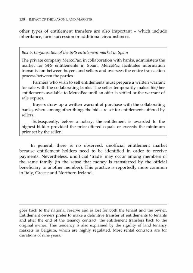
138 | IMPACT OF THE SPS ON LAND MARKETS
other types of entitlement transfers are also important – which include inheritance, farm succession or additional circumstances.
Box 6. Organisation of the SPS entitlement market in Spain
The private company MercoPac, in collaboration with banks, administers the market for SPS entitlements in Spain. MercoPac facilitates information transmission between buyers and sellers and oversees the entire transaction process between the parties.
Farmers who wish to sell entitlements must prepare a written warrant for sale with the collaborating banks. The seller temporarily makes his/her entitlements available to MercoPac until an offer is settled or the warrant of sale expires.
Buyers draw up a written warrant of purchase with the collaborating banks, where among other things the bids are set for entitlements offered by sellers.
Subsequently, before a notary, the entitlement is awarded to the highest bidder provided the price offered equals or exceeds the minimum price set by the seller.
In general, there is no observed, unofficial entitlement market
because entitlement holders need to be identified in order to receive payments. Nevertheless, unofficial ‘trade’ may occur among members of the same family (in the sense that money is transferred by the official beneficiary to another member). This practice is reportedly more common in Italy, Greece and Northern Ireland.
goes back to the national reserve and is lost for both the tenant and the owner. Entitlement owners prefer to make a definitive transfer of entitlements to tenants and after the end of the tenancy contract, the entitlement transfers back to the original owner. This tendency is also explained by the rigidity of land tenancy markets in Belgium, which are highly regulated. Most rental contracts are for durations of nine years.
EU LAND MARKETS AND THE COMMON AGRICULTURAL POLICY | 139
Consistent with the theory, regional variations in the market price of entitlements follow the variations in the face value of entitlements. This is reported to be the case in most EUSCs.59
8.1.1 Explaining transactions with entitlements Based on the theoretical results presented in chapter 2 and appendix 2, three main factors may lead to the trade of entitlements: i) a dynamic effect associated with structural change, ii) the situation in which farmers own more entitlements than they have eligible area and iii) decoupling.60
There are critical differences between the historical model and the hybrid model. Especially at the start of SPS implementation, the trade of entitlements in countries that implemented the historical SPS model was likely to be driven by structural change, because entitlements were allocated based on land used in the reference period (2000–02) and the SPS was implemented several years later (2005–06). This may have been reinforced by the decoupling that accompanied the introduction of the SPS.
Drawing from the theoretical results, in a static environment there is no incentive to trade entitlements because farms do not have an incentive to adjust land use. Entitlement trading may occur in a dynamic situation, however, which entails structural change. This point also holds for the circumstance in which the allocation of the SPS entitlements among farms is not based on land allocation at the time the SPS was introduced, but on a past equilibrium of land allocation. With the hybrid model, the allocation of entitlements was based on the total eligible area in the first year the SPS 59 In England, there is observed variation in the value of entitlements. Lower-value entitlements tend to trade at higher multipliers than the higher-value entitlements. This is partially because tenants who did a deal with their landlords to return land with entitlements are buying lower-value entitlements to give back to the landlord (keeping the higher-value entitlements for themselves). In addition, people appear to be willing to pay more for an entitlement that is rising in value (to the flat rate in 2012) than one falling in value (where there is a significant historical element), but some commentators suggest this is often a false economy because of failure to adequately discount future SPS income streams. 60 The decoupling of direct payments may lead to adjustments in the production structure and land allocation, and thus to entitlement trading. This effect is expected to be more prominent in countries with a higher rate of decoupling such as Germany, Ireland, Sweden and the UK (Table 20).

140 | IMPACT OF THE SPS ON LAND MARKETS
was applied. As a result, if structural changes occurred between the periods 2000–02 and 2005–06, then one would expect more entitlement trading with the historical model than with the hybrid model in the first years of SPS implementation.
Because under the hybrid model entitlements were allocated based on the land used when the SPS was launched, entitlement trading would not have occurred as a result of structural change. Under the hybrid model, trade may have emerged at the start of SPS implementation only as a result of decoupling. The decoupling of subsidies from production may have led farms to reallocate land and entitlements with it. Additionally, entitlement trading will likely have been affected by the fact that more entitlements were allocated with this model than with the historical model. Therefore, it is more likely that a situation would arise whereby reallocated land induced by the decoupling is used for activation of entitlements, which stimulates entitlement trading. In this case, the entitlement would accompany land.
Given that under the hybrid model more entitlements were allocated than under the historical model, it is more probable that farms would own more entitlements than the eligible area under the hybrid model. Again, this may stimulate trade. Yet in this circumstance, the entitlement would not accompany land. But if farmers trade entitlements without land, under the hybrid model the size of the entitlement market depends on the availability of entitlement buyers having naked land. If there are few or no buyers with naked land relative to the number of sellers with extra entitlements, then the volume traded will be small. Still, the pressure on entitlement sellers to trade entitlements will be reflected in higher land prices and lower market prices for entitlements (as later discussed).
The evidence from country studies partially confirms this explanation. In Germany, which implements the hybrid model, the market for entitlements is smaller in relative terms than in countries with the historical model such as France, the Netherlands or Belgium (Table 15). Indeed, the main reason farmers trade entitlements in France and the Netherlands is to match area change since the reference period with the number of entitlements they receive. On the other hand, the entitlement market is large in Sweden, which like Germany applies the hybrid model – an outcome that goes against theoretical expectations. That being stated,

EU LAND MARKETS AND THE COMMON AGRICULTURAL POLICY | 141
the value reported in Table 15 is over-estimated because of double counting.61 The prevalence of entitlement trading in Sweden may be the result of decoupling, which could have induced land-use adjustments and hence entitlement trading. Finland, similarly applying the hybrid model, also has a relatively large volume of entitlement trading, which is again against theoretical predictions.
Greece appears to confirm the static effect of the theoretical results. The land markets are rigid in Greece, particularly sales markets, because of the social value attached to land ownership. Not many land transactions take place. Hence, there is no reported, significant market for the trade of entitlements. Trade takes place mostly among family members. Transfers may occur through early retirement or unexpected circumstances (e.g. inheritance).
The low level of entitlement trading in Spain, which implements the historical model, could be attributable to tighter constraints on entitlement trading (see Table 13) and the lower rate of decoupling.
Furthermore, because the trade in entitlements stems from dynamic effects (structural changes and decoupling), sellers of entitlements are normally exiting farmers or farms in decline, while buyers are expanding or new farms.62 For example, in Sweden non-farming landowners who re-enter agricultural activity and (mainly young) farmers who embark on it tend to be buyers of entitlements. The sellers are often retiring farmers and exiting tenants. In Italy, entitlements are generally sold by retiring farmers and bought by large farms, which also holds true for Germany, where purchasers tend to be farms larger than 25 hectares (see Box 7).
61 Since transferred entitlements in Sweden as reported in Table 15 include all different kinds of transfers, a single entitlement could be transferred twice. It could, for instance, be sold and then rented in the same year. Thus, it is not possible to estimate how many entitlements were traded. In other words, the number of entitlements that have been objects of exchange among the total number of activated entitlements is smaller than what is indicated in Table 15. 62 These characteristics also imply that in general, the concentration of entitlement ownership follows structural changes. This was observed in most of the EUSCs, especially in Belgium, France, Finland and Germany.

142 | IMPACT OF THE SPS ON LAND MARKETS
Box 7. Transfers of entitlements in Germany
In 2006–07, most of the entitlements were transferred in the course of farm successions (roughly 40%) or market transactions (40%). At least half of the market transactions were induced by changes in the farmed area of the respective farms. The rest of the transactions (around 20%) were rental exchanges. The trade in entitlements decreased from 2006 to 2007, especially after it became clear that set-aside and non-permanent fruits, vegetables and starch potatoes were being abandoned (Zentrale InVeKos Datenbank).
Entitlement trading predominately takes place at the local level. The distance between the locations of the buyer and seller is less than 10 km for over 90% of the traded entitlements. Consequently, a significant reallocation of entitlements could not be observed across municipalities. Set-aside entitlements are traded slightly more often than normal entitlements.
According to the expert survey conducted by Röder and Killian (2008) and by the German team for this study, the market value is mainly between 1.0 and 1.5 times the face value of an entitlement (Table B1). This range is much lower than the net present value of an entitlement. Regarding regional variation, the survey shows that in general there is very little to speak of, whereas the market value is a little bit higher in East Germany compared with West Germany.
Table B1. Market value of traded entitlements in Germany
Region
Market price of entitlements/ face value of entitlement
(Face value of entitlement=1) Schleswig-Holstein 1.5 Lower Saxony & Bremen 1.3 North Rhine-Westphalia 1.3 Hessen 1.3 Rhineland -Palatinate 1.0 Bavaria 1.4 Saxony 1.8
Sources: Röder and Killian (2008) and the country report for Germany for this study.
At the same time, one would expect entitlement trading when
farmers own more entitlements than they have eligible area. Figure 26 shows the correlation between naked land and trade in entitlements. The higher the share of distributed entitlements relative to the total eligible area (the less there is naked land), the higher is the trade in entitlements. With

EU LAND MARKETS AND THE COMMON AGRICULTURAL POLICY | 143
less naked land, it is more likely that some farms may end up with more entitlements than eligible area. This circumstance may also be induced by structural changes or decoupling. It stimulates farms to sell entitlements in order to be able to benefit from the SPS.63
Yet, restrictions on entitlement trading may constrain this process. Figure 27 shows that in countries with more restrictions (e.g. France and Spain), entitlement trading occurs less often compared with countries with fewer restrictions (e.g. Belgium, Finland and the Netherlands). In Germany, the volume of entitlement trading is low, owing to adoption of the hybrid model, which led to less entitlement trading at the start of SPS implementation. In the UK, selling fees charged by market agents for transfers appears to make the trade less viable.64
In Northern Ireland, the trading volume is very low probably because of the possibility to consolidate entitlements. Farmers were permitted to consolidate the historical component of the entitlement value onto a smaller area to increase the unit value of their entitlements. This reduced farmers’ surplus entitlements. A similar development is expected in Ireland but data are not available to confirm this (see Box 9 in section 8.2.1.1 below).
When trade in entitlements is induced by structural change and decoupling, then entitlement transfers will always be accompanied by land. For example, if a farmer becomes less profitable as a result of structural change, the farmer is more likely to reallocate land and entitlements with it. In instances where farmers own more entitlements than they have eligible area, transferred entitlements normally will not be accompanied by land. A farmer with extra entitlements would be more willing to either sell 63 When analysing the data presented in Figure 26, caution should be applied owing to the quality and consistency of the data. Data on the trade of entitlements include various kinds of transactions and the data themselves come from diverse national sources – all of which poses problems of consistency and comparability among countries. Also, it is difficult to draw robust statistical conclusions from the few available observations. 64 The ranking of restrictions presented in Figure 27 only takes into account regulatory restrictions. Other non-regulatory restrictions (e.g. credit constraints or an underdeveloped entitlement market) are not taken into consideration, as consistent information is not available. Such information could considerably improve the analysis.

144 | IMPACT OF THE SPS ON LAND MARKETS
entitlements or acquire additional land without entitlements in order to activate all the subsidies. The evidence from country studies shows that entitlements are most often traded with land – when land is sold or rented by another farmer – in most EUSCs. Based on the available information, a significant difference cannot be identified between the hybrid and the historical models. This confirms that structural change and decoupling tend to be the major influences on the market for entitlements.65
In Spain, where entitlements are traded both with and without land, the entitlements traded with land slightly exceed those transferred without land. In France, tight restrictions on entitlement trading have discouraged transfers without land (i.e. 50% of the entitlements traded without land revert to the national reserve).
In contrast, in Belgium transfers without land are the most frequent because they are administratively the least costly. This pattern similarly holds in the study region Saxony. Unlike the rest of Germany, in Saxony land and SPS entitlements are bought and sold through different channels. In Scotland, the transfer of land and the SPS entitlements are also two separate transactions. The segregation could be explained by many farmers owning more entitlements than eligible area – a reason reinforced in Table 12, which shows that there is no naked land available in Scotland.
8.1.2 Explaining the market price of entitlements With perfect markets, one would expect that the price of an entitlement would equal the net present value of the future stream from that entitlement. For example, with a discount rate of 10% and if we assume that the SPS runs until 2013, the market value of an entitlement in 2007 should
65 Caution should be applied in interpreting these results. As noted earlier, in cases where farmers own more entitlements than they have eligible area, farmers are willing to either sell entitlements or acquire additional land without entitlements. More specifically, land transactions induced by farmers who own extra entitlements cannot be exactly quantified based on available data. There is some evidence that the hybrid model, where this problem most likely occurs, tends to stimulate land transactions (see the next sections for more details).

EU LAND MARKETS AND THE COMMON AGRICULTURAL POLICY | 145
be 4.4 times higher than its face value, while if the SPS runs indefinitely then the market value of an entitlement in 2007 should be 10 times higher than its face value.66
Table 16 shows that the market price of an entitlement in most EUSCs is between 1.0 and 3.0 times higher than the face value of that entitlement. These figures are significantly less than the theoretical expectations. Three factors may explain the observed gap in the entitlement price between theory and empirical evidence.
First, there is uncertainty about the duration of the SPS. In general, farmers’ expectations are that the SPS will run until 2013. Additionally, there is hesitation associated with the possibility of further reforms to the historical model, which reduces the market price of entitlements. For example, according to expert estimates the market price of entitlements was up to 6.0 times the face value in France in 2006, but it declined to between 1.0 to 1.5 times mainly because of the uncertainty about the post-2013 SPS. In England, because modulation rates were unknown in England until 2007, there was considerable vagueness in the market concerning the potential income streams from entitlements. Moreover, uncertainty in the market was also brought about by the euro–sterling exchange rate and the CAP health check. These uncertainties are among the reasons for the small size of the entitlement market in England.
Second, imperfections in credit markets reduce the value of entitlements. If potential buyers face financial constraints, they cannot afford to pay the net present value of entitlements, even when they have perfect expectations.
A third factor leading to lower market prices compared with theoretical expectations is the additional costs connected with receiving the
66 With a discount rate of 5%, the market price of an entitlement in 2007 should be 5.1 times higher than its face value if the SPS runs until 2013, and 20 times higher than its face value if the SPS runs indefinitely. We note that these calculations do not take into account the impact of modulation (expectations of an increased rate of modulation) and farm administrative costs or other additional costs that the SPS may induce.

146 | IMPACT OF THE SPS ON LAND MARKETS
SPS subsidies, which may be induced by cross-compliance67 and administrative costs, as well as by taxes and fees imposed on entitlement transactions. Anecdotal evidence from the Netherlands indicates that in situations where both land and entitlements are rented in combination, approximately 5-10% of the nominal entitlement value is deducted from the rental price. This discount could be partially explained by a) the administrative costs of applying for the payment; or b) an implied interest rate as rental contracts are signed in November, but the related subsidies are paid out a few months later in the spring; or c) a risk discount.
The retail price for entitlements in the study region of Emilia Romagna is in the range of 30-50% of the annual payment. Based on a survey of over 1,000 farms in five different regions in Germany, the rental price for entitlements is between 0% and 20% of the face value of the SPS. This may also indicate the presence of high additional costs, as rent is an annual payment and is affected to a lesser extent by traders’ expectations about the future continuation of the SPS. In Greece, there are still mistakes in the administration of the SPS system, which constrain the entitlement market.
In summary, the low price of entitlements may indirectly indicate the existence of market imperfections and rigidities and hence its underdevelopment. With better functioning markets one would expect higher prices and larger traded volumes than reported in Table 15 and Table 16, respectively.
67 According to the EU regulations, all land utilised by farms must respect cross-compliance criteria irrespective of whether it is used for the activation of entitlements. If a farm buys an entitlement without land and activates the entitlement using land that was already at a farm’s disposal before the purchase of the entitlement, it is not expected to incur additional costs for the farmer. This is because the cross-compliance requirements must be respected with or without using the land for activation of the purchased entitlement. But if the farmer buys an entitlement and land, then it may happen that cross-compliance leads to additional costs for the farmer. This situation is more likely to occur in relation to land of low fertility, which a farm may purchase together with the entitlement just to keep it in GAEC and thus benefit from the purchased SPS. Studies have shown that the burden of cross-compliance tends to be positive but relatively small (e.g. European Commission, 2007c).

EU LAND MARKETS AND THE COMMON AGRICULTURAL POLICY | 147
On the other hand, the low price of entitlements may indicate their capitalisation into land values. Based on theoretical results, SPS land capitalisation may accrue with dynamic effects, with new entrants being eligible for entitlements and in scenarios where the total eligible area is smaller than the total number of entitlements (i.e. with a low level of naked land).
Figure 28 shows the correlation between naked land and the market price of entitlements. The higher the share of distributed entitlements relative to the total eligible area (the less there is naked land), the higher is the market price of entitlements. This outcome goes against theoretical expectations. One would expect the opposite relationship between naked land and entitlement price. This could stem from the fact that as naked land is still substantial in most reported countries in Figure 28, there is no significant capitalisation of the SPS into land values, especially in countries applying the historical SPS model.68 The quality of data may also affect the results, given that many of the prices presented in Table 16 are expert estimates. At the same time, the eligibility of new farmers is not expected to be a key factor in SPS capitalisation, as a significant number of entitlements for entering farmers were not granted. Still, the low price of entitlements could indeed be the outcome of rigidities in the market for entitlements combined with dynamic effects, which may induce SPS capitalisation (as discussed in the next section).69
68 Fallow land could reduce the pressure of low levels of naked land on entitlement market prices. For example, in Italy there was extensive abandonment of land in some parts of Italy between 1982 and 2000. This land can easily be brought into cultivation or be used to activate entitlements. According to Eurostat data, the shares of fallow and green manure land in the UAA are broadly as follows: 0% in Ireland; 1-5% in Belgium, Germany, Greece, France, Italy and the Netherlands; 10% in Finland and Sweden; and 14% in Spain. 69 When analysing the data presented in Table 16 and Figure 28, one must take in consideration the quality of data. In several countries, entitlement prices are based on market experts’ estimates. It is difficult to draw statistical conclusions from the few available observations.

148 | IMPACT OF THE SPS ON LAND MARKETS
There is some evidence that in countries with the historical model, entitlement prices are higher than in countries with the hybrid model. For example, in the UK, entitlement prices are substantially higher in Scotland (historical model) than in England (hybrid model). Similarly, in Belgium, Ireland and the Netherlands (historical model) it appears that entitlement prices are higher than in Germany (hybrid model) (Table 16). Theoretically, the historical model leads to lower capitalisation of the SPS than the hybrid model. As a result, entitlement buyers are willing to pay a higher price for entitlements in countries with a historical model than is the case in countries with a hybrid model.
8.2 Impact of the SPS on land markets This section analyses the impact of the SPS on sales and rental markets for agricultural land. We separately examine the impact of the SPS on land transactions (trade) and the extent to which the SPS becomes capitalised into land values. This section also analyses the distribution of benefits from the SPS between farmers and landowners and the effect of shifting the SPS to a regional model.
8.2.1 Impact of the SPS on land transactions In a static environment, the SPS does not affect land transactions (sales and rentals). The same holds in the dynamic context with structural change and the full tradability of entitlements. Theoretically, land transactions induce the trade of entitlements and not vice versa. Land transactions arise if there is structural change, decoupling and farm exit. These factors lead to land reallocation among farms. If the relocated land is used to activate entitlements and if entitlements are fully tradable, then entitlements will accompany land transactions.
Yet, if the trade of entitlements is constrained, then land transactions may be affected. In this case, the SPS restricts land transactions. With constrained trade, farms that want to reallocate land and dispose of an equivalent number of entitlements cannot sell their entitlements for the desired price. For this reason, these farms may reduce the total amount of reallocated land to avoid losing the benefits from the SPS entitlements.

EU LAND MARKETS AND THE COMMON AGRICULTURAL POLICY | 149
Additionally, the SPS may stimulate land transactions when farms have a smaller eligible area than the total entitlements allocated. To be able to activate entitlements, farms search for land on either the sales or the rental markets. This effect increases the total number of land transactions.70
Administrative regulations and details associated with implementing the SPS may affect land transactions as well as the kinds of sales and rental contracts used. For example, landowners interested in obtaining SPS entitlements may cancel their contracts with farmers and apply for the SPS entitlements themselves. If implementation of the SPS requires proof that the farm uses rented land, this stipulation may lead to more written rental contracts. These effects, however, depend on the extent to which land markets are developed and regulated, and on the SPS model.
In summary, the overall effect of the SPS on land transactions (trade) is ambiguous. Constrained tradability of entitlements combined with structural change reduces land transactions while a smaller eligible area than the total entitlements allocated stimulates land transactions.71 Administrative regulations can affect land transactions in either direction. With respect to the historical SPS model, one should expect that it decreases the total number of land transactions because one of the main drivers of land transactions is structural change. Under the historical model, entitlements are allocated based on the subsidies farms obtained in the reference period 2000–02, while the SPS was implemented in the period 2005–06. If in this period structural change occurred (combined with decoupling), this may lead, for example, to the reallocation of land and farm exit, which could be limited by the SPS if entitlements are not fully tradable. Hence, in this case the SPS would reduce land transactions. In contrast, the hybrid model is expected to stimulate land transactions. 70 In this scenario, the SPS may affect the use of abandoned land, as farmers may use fallow land to activate entitlements. 71 Nevertheless, this depends on the availability of naked land. If there is little or no naked land available relative to the number of farms with extra entitlements that want to buy or rent land, then the effect of the SPS on land transactions will be small. But the pressure will be reflected in higher land prices and lower market prices for entitlements (for more details, see the later section on the impact of the SPS on land values). Table 12 shows that in several countries, a substantial amount of naked land is available, chiefly in countries that apply the historical model. In countries with the hybrid model, less naked land is available.

150 | IMPACT OF THE SPS ON LAND MARKETS
Compared with the historical model, there are more entitlements allocated under the hybrid model, while the effect of structural change on land reallocation is smaller at the beginning of SPS implementation.
Next, the evidence on the impact of the SPS on land transactions is discussed. Sales and rental transactions are examined separately. Still, one should keep in mind the data limitations. More specifically, data on land transactions are scarce for the period following the launch of the SPS. Meanwhile, during this period agricultural prices rose, and this may have affected land transactions. This price effect reduces the possibility to single out the impact of the SPS on land transactions.
8.2.1.1 Sales transactions In general, evidence from the study countries shows that the SPS has had little or no impact on land sales transactions. Survey data for France especially confirms this finding (see Table 12 and Box 8), which show that there has been no significant effect of the SPS on farmers’ preferences regarding land purchases. Nor is there evidence that the SPS has affected land transactions in Germany or Sweden. In the Netherlands and Northern Ireland, it is difficult to isolate the effect of the SPS on land sales transactions, as other factors are much stronger drivers.
Consistent with the theoretical model, the SPS provides some incentives to own land in Finland, which implements the hybrid model. This could stem from the low level of naked land (Table 12), which motivates farmers to own land in order to activate all of their entitlements. Germany and Sweden likewise implement the hybrid model, and thus a positive effect of the SPS on land sales transactions should also be expected. But the level of naked land is higher in these two countries (especially in Germany) than in Finland, which mitigates the effect of the SPS on land transactions. The evidence shows a small or no impact of the SPS on land sales transactions in these two countries.
There is some evidence that in countries that have implemented the historical model the SPS tends to dampen land sales transactions (e.g. Belgium). Exiting farmers prefer to keep land in order to receive the SPS payments. In addition, the low market price of entitlements reduces the incentive of exiting farmers to sell the entitlements. In Spain, many sales transactions were delayed until the exact entitlement transfer procedures were known.

EU LAND MARKETS AND THE COMMON AGRICULTURAL POLICY | 151
Box 8. Impact of the SPS on land transactions in France
There has been no significant impact of the SPS on farmers’ preferences regarding renting or purchasing land in France. This has been confirmed by the survey conducted under the European Commission’s FP6 research project IDEMA. The results are shown in Table B2, which indicate that the number of French farmers (among 281 respondents) intending to purchase or rent in land is similar under the three scenarios considered: i) continuing the policies of Agenda 2000, ii) real implementation of the 2003 reform and iii) full decoupling (Douarin et al., 2007).
Table B2. Number of farmers intending to decrease or increase their current farm area (average number of hectares envisaged in brackets)
Scenario 1: Continuing
Agenda 2000
Scenario 2: Implementing
the 2003 reform
Scenario 3: Hypothetical
full decoupling
Decrease their current farm area by
Selling land 0 (-) 0 (-) 0 (-) Reducing land rented in 0 (-) 0 (-) 0 (-) Increasing land rented out 0 (-) 0 (-) 0 (-) Passing on land to a successor 2 (60 ha) 2 (60 ha) 2 (60 ha) Converting land to non-agricultural uses 2 (5 ha) 3 (4 ha) 3 (4 ha)
Increase their current farm area by
Purchasing land 28 (42 ha) 26 (44 ha) 26 (44 ha) Increasing land rented in 65 (33 ha) 66 (33 ha) 57 (33 ha) Decreasing land rented out 1 (60 ha) 1 (60 ha) 0 (-) Converting land from non- agricultural uses 1 (10 ha) 1 (10 ha) 1 (10 ha)
Source: Douarin et al. (2007), Tables 8-26.
Yet because of the complexity of the SPS, it seems that older farmers who were not eligible for the SPS exited the farming sector earlier than they would have done if Agenda 2000 had continued. This may have led to a greater amount of trade in land, shortly before and during the first years of SPS implementation. Some farmers may have postponed their exit, however, in order to benefit from subsidies that are certain for the next few years. Thus, the net overall impact of the SPS on the number of sales transactions is not clear.

152 | IMPACT OF THE SPS ON LAND MARKETS
In Italy, two effects have been observed. First, the uncertainty brought by the CAP reform has reduced land sales transactions, while the requirement to have land to activate entitlements has increased activity in the land sales market. This second effect appears to be temporary, however.72 In the study region Emilia Romagna, the impact of the SPS on agricultural land sales transactions is very low, although plots with entitlements are more commonly traded than plots without them.
In Scotland, there was a significant decline in the traded area in 2004, perhaps stemming from uncertainty about the rules to be applied in SPS implementation.
In Ireland, there is no clear indication of whether the SPS affects the incentive to own agricultural land. One can only speculate that the effect of the SPS may have led to a freezing of land ownership, at least at the start of SPS implementation. This conjecture could especially apply to farms that consolidated their SPS entitlements. Consolidation could not be carried out by farmers who disposed of their land by sale or lease (see Box 9).
Box 9. Consolidation of entitlements in Ireland
The requirement that individual farmers must have 100% of the average land area that they had in the reference period would have resulted in serious problems for those farmers who, for specific reasons, declared less land in 2005 or in subsequent years than the average area of land they had cultivated in the reference period.
Under the provisions of the EU regulations, a member state may make use of its national reserve to consolidate payment entitlements for certain categories of farmers on the actual number of hectares of land farmed in 2005. This process entails surrendering the original entitlements to the national reserve in exchange for a lower number of entitlements with a higher unit value. Note that the overall value of the payment is not affected.
72 Its temporary character is also indicated by the fact that in most cases entitlements and land are traded together. The volume of entitlement trading in which land is withheld is rather small.

EU LAND MARKETS AND THE COMMON AGRICULTURAL POLICY | 153
Box 9. cont’d
The requirement that individual farmers must have 100% of the average land area that they had in the reference period would have resulted in serious problems for those farmers who, for specific reasons, declared less land in 2005 or in subsequent years than the average area of land they had cultivated in the reference period.
Under the provisions of the EU regulations, a member state may make use of its national reserve to consolidate payment entitlements for certain categories of farmers on the actual number of hectares of land farmed in 2005. This process entails surrendering the original entitlements to the national reserve in exchange for a lower number of entitlements with a higher unit value. Note that the overall value of the payment is not affected.
The farmer must declare the entire agricultural land available to him in 2005 and the total area declared must be equal to at least 50% of the average area declared during the reference period. The farmer may apply for the concession in a particular year provided (s)he continues each year to declare at least 50% of the land area farmed during the reference period.
The concessions relating to consolidating entitlements cannot be applied to farmers who declare fewer hectares than entitlements because the remaining land has been sold or rented out. One exception is where land is purchased by a public authority for non-agricultural use (e.g. for road construction). In such cases, the consolidation of entitlements is possible.
According to the Irish Department of Agriculture, Fisheries and Food, the entitlement consolidation provisions may be applied to farmers who • afforested some of their land after the reference period began; • disposed of their land to a public authority for non-agricultural use; • had leased/rented in land during the reference period, for which the
agreement has since expired; or • declared land situated in Northern Ireland during the reference
period. Where a farmer benefits from this concession, all of his/her
consolidated payment entitlements will be regarded as having come from the national reserve. The entitlements concerned cannot be sold or leased out for at least five years from the year of allocation. Moreover, the farmer must use all of his/her entitlements him-/herself each year for a period of five years or the unused entitlements will revert to the national reserve.

154 | IMPACT OF THE SPS ON LAND MARKETS
The SPS has also led to adjustments in land sales contracts. Clauses have been added in the sales contracts to regulate who receives entitlements that accompany land or to specify whether entitlements are sold together with land (e.g. France and Germany). Furthermore, the SPS has led to land market segmentation between land traded with and without entitlements, with price differences between them (e.g. France and Italy).
8.2.1.2 Rental transactions The evidence from the EUSCs suggests that the impact of the SPS is stronger on land rental than sales transactions. Yet, there are also notable differences in terms of the SPS effects. In particular, there is a difference between the historical and hybrid models. The hybrid model has induced some marked effects on land rental markets. Specific features of the hybrid model allow non-farming landowners to access SPS subsidies in the hybrid model, while this is possible to a lesser extent under the historical model.
With the hybrid model, the number of entitlements that farmers have received is equal to the total eligible area in the first year of SPS application. Landowners who rented out land prior to the introduction of the SPS could gain access to entitlements by either cancelling the rental contract and applying for entitlements themselves or by adjusting rental contracts in order to ensure that entitlements revert to the landowner after the contract expires. This aspect of the hybrid model has enabled some non-farming landowners to obtain entitlements. And in several countries that have implemented the hybrid model, non-farming landowners have indeed done so, thus benefiting from the SPS.
For example, in Sweden, which implements the hybrid model, the total rented area decreased between 2003 and 2005 by around 10%.73 Previously, renting had exhibited a long-term upward trend (although there was considerable regional variation). The reduction was much more pronounced in the southern, fertile regions than in the north. One possible explanation is that landowners in the south tend to live closer to their land
73 The introduction of the SPS initially brought turmoil to the rental market in Sweden but the market eventually adjusted to the new institutional framework. The turmoil ensued because entitlements were allocated to those who cultivated the land at the time the SPS was introduced, and some landowners wanted to terminate rental contracts in order to receive the entitlement payments themselves.

EU LAND MARKETS AND THE COMMON AGRICULTURAL POLICY | 155
and could therefore return to farming or land management and obtain entitlements. In northern Sweden, absentee landowners are usually farmers who have quit farming and have moved south, as alternative income opportunities are scarce in the region.74 Furthermore, it appears that in another respect the ultimate beneficiaries of the SPS are landowners. The new land rental contracts that are being written nowadays always include a clause stating that the entitlements will go back to the landowner when the contract is terminated.
Likewise in Finland (hybrid model), based on interviews with local officials, the common procedure is that the SPS entitlements are returned to the landowner when the rental contract expires. With the introduction of the SPS, most of the rental contracts have been renewed with this modification.75 The level of the rent has typically stayed the same. Some landowners did not renew contracts that expired in 2005, to ensure that they received the entitlements in 2006 when the SPS was introduced in Finland (see Box 12 in the section 8.2.2.2).
In Northern Ireland (hybrid model), non-farming landowners could, in certain circumstances, apply to establish entitlements relating to the land they own (the regional component of €78.33/ha), even if they had never historically received direct support payments. To do so, they had to apply for a business reference number on or before 16 May 2005 and submit an application form by that same date. By establishing and claiming entitlements, non-producing landowners must assume the responsibility for meeting the cross-compliance obligations for their entire land holding, even if this land is cultivated by a tenant.
In England (hybrid model), rental arrangements between farmers and landowners were made to return land with the associated entitlements. Data are not available to quantify the share of the area covered by such arrangements. Decoupling also had some effect on rental transactions in England. Under the old extensification scheme, land that was rented was
74 Consequently, the SPS has introduced distortions. Landowners who did not farm their land prior to SPS implementation began doing so and replaced incumbent farmers. 75 This practice involved around 30% of entitlements, which is equivalent to the share of rented land in Finland. The rest of entitlements (around 70%) are owned by landowning farmers and thus no contractual adjustments were required.

156 | IMPACT OF THE SPS ON LAND MARKETS
often not grazed as farmers sought to maximise subsidy payments under the old coupled, CAP support system. Under the SPS, less grazing land is rented, since there is no requirement under extensification rules. In England, there was additionally a significant swapping of land to ensure that the entitlements were not lost (e.g. potatoes and peas being ineligible meant that parcels of land needed to be swapped to ensure farmers renting land for these crops did not lose out under entitlements). This also had an impact on tenancies and specifically grazing agreements (i.e. people were effectively selling grass and not leasing land, in order to claim entitlements).
In Germany, which also implements the dynamic hybrid model, such tendencies among landowners were not observed. The results of surveys conducted in three case study regions suggest that the number of non-farming landowners who applied for the SPS entitlements is marginal. Two factors explain this outcome. First, this practice is constrained by the prevalence of long-term rental contracts with an average duration of 7-12 years. Second, the existence of a clear regulation on the ownership of entitlements after rental contracts expire does not allow non-farming landowners to obtain entitlements. According to the decision of the Federal Court of Justice on 24 November 2006 (no. LwZR 3/06), tenants can retain entitlements even after the expiry of rental contracts. Still, there are indications that large landowners (e.g. the Protestant Church in Lower Saxony) use their strong bargaining position to obtain entitlements in Germany (e.g. by obliging farmers to accept the reassignment of entitlements after the expiry of rental contracts). Although not representative of all regions, such phenomena may be highly significant at the local level in some regions.
In countries that have implemented the historical SPS model, the number of entitlements that farmers received depends on the subsidies and the eligible area in the reference period (2000–02). For this reason, only those who were farmers in the reference period and receive subsidies then could become owners of entitlements, cutting out non-farming landowners without a farming record or proof of subsidies received in the reference period. These conditions reduced the power of non-farming landowners to acquire entitlements through change or cancellation of rental contracts. Evidence from several study countries applying the historical model suggests that the SPS has had little or no effect on land rental transactions (e.g. France, Italy and the Netherlands).

EU LAND MARKETS AND THE COMMON AGRICULTURAL POLICY | 157
In Belgium and Spain, which have likewise implemented the historical model, there is some evidence that the SPS constrains land rental transactions – similar to what has been observed for land sales markets. This effect can be traced to structural change and the imperfect tradability of entitlements, which results in a low market price for entitlements. The low market price in turn reduces the incentive of farmers to reallocate land if the respective land is used for the activation of payments. Farmers who want to reallocate land and entitlements with it (e.g. retiring or exiting farmers) prefer to continue using land and benefiting from the SPS rather than lose out in this respect. This is most evident in Belgium, where the SPS reduces land rental transactions and reinforces the effect induced by rigid rental-market regulations (see Box 10).
Box 10. Impact of the SPS on land markets in Belgium
Land rental markets are tightly regulated in Belgium. In general, there are two kinds of tenancy contracts: regular contracts and seasonal contracts. Regular contracts can be of a duration no shorter than nine years and the maximum rent that landowners can charge tenants is regulated. Seasonal contracts are for periods of less than a year and the rent can be set freely.
On the one hand, regular contracts give farmers security. On the other hand, they constrain the restructuring process as a dynamic farmer (e.g. young farms) has more difficulty in accessing land (as land is locked in long-term rental contracts). Seasonal contracts offer flexibility in terms of rental rate-setting but offer farmers little security. To side-step regulations, informal transactions take place (e.g. payment of an additional premium in excess of the official maximum rent allowed under regular contracts) as well as the seasonal contracts that are preferred by landowners.
The SPS is an additional factor that may constrain restructuring. Upon retiring or exiting, landowning farmers prefer to keep their land to enable them to activate entitlements. The low market price of entitlements reduces the incentive for retiring or exiting farmers to sell them. To benefit from the SPS, it is sufficient to hire services just to keep their land in good agricultural condition. This custom further reduces the available land on the rental market. Expanding farms are therefore willing to bid more for rents to gain access to land. The effect is that farmers engage more in the seasonal and informal contracts, by which landowners can demand higher rent or additional premiums for regular contracts on top of the maximum rent allowed.

158 | IMPACT OF THE SPS ON LAND MARKETS
Box 10. cont’d
Furthermore, given the long-term tenancy contracts, some farmers may have difficulty in finding available land to activate their entitlements. This situation puts upward pressure on escalating land rents for seasonal contracts and premiums for regular contracts.
The SPS affects the sales market in a similar way as the rental market, but the effect is weaker because the sales market is less regulated and other factors influence land sales prices to a greater degree.
In summary, the SPS is reinforcing the problem induced by a rigid rental market, which constrains restructuring. At the same time, the SPS is partially becoming capitalised into land rents.
In Spain, exiting farmers prefer to continue renting land in order to
receive the SPS payments. Low market prices for entitlements and high transfer taxes reduce the incentive to sell the entitlements. In some cases, farmers who are also landowners and own entitlements prefer to rent the land out through an unofficial market for free or at a very low rate in exchange for the tenant keeping the land in GAEC. Thus, the landowner uses land to activate the entitlement while the farmer uses the land for production. This allows the landowning farmers to benefit from the SPS. In Spain, the share of naked land is high (Table 12), thus ensuring that tenants can find sufficient eligible area for activation of their own entitlements.
The effect of the SPS on land rental transactions is very small in Ireland. This result is mainly attributable to the possibility of consolidating entitlements on a smaller area than that used in the reference period, as noted above. This action reduced pressure on land markets in general. The possibility to consolidate entitlements on a smaller area eased pressures arising from structural changes that took place between the reference period (2000–02) and the time the SPS was introduced (2005) and from the low level of naked land. Instead of being forced to search for land in order to activate entitlements, farmers could reduce the number of entitlements without reducing the total value of subsidies. A similar situation has been observed in Northern Ireland, where the ‘stacking’ facility is also applied.
An important consequence of the SPS is the spreading formalisation of rental contracts (e.g. Germany, Italy, Spain and Sweden). For the most part, to benefit from the SPS, farmers are required to provide documentation to support that they farmed the area used for the activation

EU LAND MARKETS AND THE COMMON AGRICULTURAL POLICY | 159
of entitlements. This requirement induced many farmers to convert oral rental contracts into written ones. The shift is particularly notable in Spain. Concerning the duration of rental contracts, only a few country studies report that the SPS has had an effect, with most reporting no impact.
In Sweden, tensions between the landowners and the tenants over the lengths of the contracts seem to have increased in recent years as reported in farmers’ professional magazines. There is a clear tendency towards shorter (one-year) contracts in the market for rented land. Most probably, this can be attributed to the introduction of the SPS.
In England, because of the SPS (and tenants claiming entitlements), many tenants have been encouraged to prolong their leases to 2012 to ensure the entitlements are enabled, so everyone has some subsidy from land.
8.2.2 Impact of the SPS on land values This section analyses the extent to which the SPS is capitalised into land sales prices and land rents. The evidence presented above showed that the price of entitlements is relatively low in the study countries (Table 16), which could be related to the presence of constraints in the tradability of entitlements (market imperfections and restrictions imposed on the trade of entitlements). The main objective of this section is to determine whether the low price of entitlements could also be connected to their capitalisation into land values. According to the theoretical results, if the SPS is capitalised into land values then the market price of entitlements declines. With full capitalisation of the SPS into land values, the market price of entitlements is zero.
Based on the theoretical results, capitalisation of the SPS into land values occurs when • the total number of entitlements allocated is larger than the total
eligible area, • new entrants are eligible for SPS entitlements, and • asymmetric structural changes occur (including farm exit and
decoupling) or there are non-tradable entitlements. The capitalisation of the SPS into land sales prices depends on the
extent to which land rents correlate with sales prices. If sales prices fully incorporate the discounted sum of future rental values, then the effect of the SPS on sales prices is equal to the effect of the SPS on rents. But if land

160 | IMPACT OF THE SPS ON LAND MARKETS
sales prices do not fully incorporate the discounted sum of future rental values, then there is less capitalisation of the SPS into sales prices than in the case of rents.
Next, the evidence on the impact of the SPS on land sales prices and land rents is presented. The short time span since the implementation of the SPS, combined with the poor quality of the available data, prevent a consistent econometric analysis. At the same time, it is more difficult to identify the impact of the SPS on land sales prices than on land rents because sales prices are driven by several non-agricultural factors and market expectations are important drivers. For land rents, this is less of a problem. Yet, rental markets tend to be more regulated than sales markets (especially in Belgium and France), and in rigid markets the contracts tend to be of a longer duration. These factors may delay or mitigate the capitalisation of the SPS into higher land rents if the effect is present.
Moreover, if previous area payments introduced by the 1992 CAP reform and by Agenda 2000 were capitalised into land values, then the impact of the SPS could be difficult to isolate.76 The literature estimating the impact of previous subsidies on land values is almost non-existent. To our knowledge, only three studies cover EU countries (Trail, 1980; Goodwin and Ortalo-Magné, 1992; Duvivier et al., 2005), with first two studies estimating the effect of the pre-1992 CAP policies. Duvivier et al. (2005) estimate the impact of the 1992 and subsequent CAP reforms on arable farmland prices in Belgium. Depending on the year and region considered, the elasticity of arable farmland prices to compensatory payments ranges from 0.12 to 0.47.
8.2.2.1 Land sales prices Particularly for land sales prices, it is difficult to identify the effect of the SPS because other factors are more influential than the SPS (such as urban
76 For example, if one assumes that previous subsidies were capitalised into land values, then land prices should have declined with the introduction of the SPS. Yet, during the period of SPS implementation, agricultural prices increased – which could have offset the effect of the SPS. Hence, to identify the effect of the SPS on land values one needs to have, among others things, good knowledge of the effect of previous subsidies and market prices on land values.

EU LAND MARKETS AND THE COMMON AGRICULTURAL POLICY | 161
pressure, agricultural prices and farm productivity).77 Compared with the other drivers of land sales prices considered in this study, the impact of the SPS has also proven the most complicated to identify and market experts have varied widely in their estimates (among countries and among regions within a country). These factors make it difficult to draw a clear conclusion about what impact introducing the SPS has had on land sales prices.
Taking into account these limitations, the evidence generally shows that the impact of the SPS on land sales prices has been relatively small: with few exceptions, there has been no significant change in land prices since SPS implementation.
The main drivers of SPS land capitalisation appear to be the small amount of naked land and structural changes (including decoupling and farm exit). New entrants’ access to SPS entitlements was not identified in any of the study countries as an important determinant of SPS capitalisation into land prices. The underlying reason here is that significant numbers of entitlements were not allocated to new entrants in any of the study countries in the period covered by the study.
There are notable differences between the SPS models. The evidence shows that the hybrid model tends to lead to greater capitalisation of the SPS into land prices than the historical model.78 Most of the countries with the hybrid model report land capitalisation of the SPS; yet, no significant effect of the SPS has been observed in several countries that have implemented the historical model. The evidence indicates that land capitalisation of the SPS is driven by the low amount of naked land in countries with the hybrid model and by structural changes in countries with the historical model. These results confirm theoretical expectations. The differential effect between the models could also be related to an under-representation of countries implementing the hybrid model.
77 On the other hand, this may suggest low capitalisation of the SPS into land prices or a low contribution of the SPS to the total price of land. Still, one should be cautious when interpreting these arguments, as they cannot be generalised. 78 It should nonetheless be noted that only five countries covered by this study implement the hybrid model. Most countries and regions implement the historical model (Table 8). One should be careful about generalising these results for the entire EU.

162 | IMPACT OF THE SPS ON LAND MARKETS
Still, if both the SPS and the previous subsidies are capitalised into land values at the same rate, then one should expect less change in land prices with the historical model than with the hybrid model, for several reasons. First, the historical model has not affected the subsidies each farm receives, while the hybrid model has redistributed subsidies among farms, sectors and regions, thus affecting land prices in some regions (above all for less fertile land). Second, agricultural commodity prices rose in parallel with the introduction of the SPS, which could have offset the potential decline in land sales prices caused by the SPS. Third, decoupling provides for flexibility on production, enabling farms to react to market signals, and hence increasing profitability and potentially land prices. This makes the impact of the SPS difficult to identify.
Based on the survey of experts, the SPS had a slightly positive impact on the development of agricultural land prices between 2004 and 2007 in Sweden (hybrid model). The most visible impact of the introduction of the SPS is the increase of (semi-natural) grassland prices in Sweden. Prices grew substantially in 2005 and 2006. More importantly, grassland prices climbed faster than arable land prices in 2005 and 2006 (Figure 29). One might expect that non-agricultural drivers of prices for grazing land would have a weaker influence in this case because such land tends to be located in less accessible areas. Also, agricultural drivers may have a small impact on grassland prices because with decoupling, this land may become abandoned. In the case of arable land, both non-agricultural and agricultural factors affect the land prices and therefore it is difficult to identify what caused the changes in prices. If this holds, then the sharp increase in grazing land prices in recent years may be the effect of the SPS driven by farmers’ demands for land in order to activate entitlements. Indeed, the evidence shows that the value of the entitlement represents the lowest threshold of the market price, reduced by the costs for keeping land in GAEC. The same ramifications of the SPS hold for land rents.
A similar effect is observed in Finland (hybrid model). Statistical evidence reveals that land sales prices were affected by the introduction of the SPS. In Germany (hybrid model), the effects of the SPS have been minor. The impact of the SPS on land sales prices has varied from low to medium. But compared with agricultural commodity prices and agricultural productivity, the influence of the SPS has been insubstantial.

EU LAND MARKETS AND THE COMMON AGRICULTURAL POLICY | 163
In Northern Ireland, there is a complete lack of land for sale, which means that when land does come on the market it attracts a very high price.79 Therefore, factors other than the SPS are driving the market.
In a number of countries that have implemented the historical SPS model, there has been little or no impact of the SPS on land sales prices (e.g. Greece, Ireland, Italy and the Netherlands).80
Greece confirms the static effect of the theoretical model. With limited activity on the sales market, the SPS has had no effect on land sales prices. Thus, the SPS is not capitalised into land values.
In Spain, statistical analysis reveals a positive correlation between land prices and the value of SPS entitlements. Yet this finding could be attributable to the historical model and the fact that previous subsidies were linked to productivity. This correlation may just reflect the policy bias, i.e. more productive land has a higher price and has received higher subsidies in the reference period, and thereby received SPS entitlements with a higher value.
Probably the strongest effect of the SPS on land sales prices in a country with the historical model has been seen in Belgium. SPS land capitalisation there is driven by structural changes and the partial tradability of entitlements. The low market price of entitlements reduces the incentive for retiring or exiting farmers to sell entitlements. For this reason, exiting landowner farmers prefer to keep the land and activate the
79 Despite the high sale values of farmland in Northern Ireland in recent years, many landowners choose not to sell land because of their desire to carry on a family tradition, where land is passed down from generation to generation. 80 Other drivers dominate land values in the Netherlands. The effect of the introduction of the SPS is difficult to quantify as other factors influence land prices much more. The real option to convert land to non-agricultural use, for instance, accounts for at least half of the (in a European comparison) extremely high Dutch land prices. Robust growth in the prices for agricultural outputs and the pressure caused by high revenues from receiving manure further reduce the share of land values depending on subsidies. Implementation of the European Nitrates Directive has probably had a higher impact on Dutch farmland prices than the move towards the SPS, as it created a new source of cash flows for both landowners and tenants.

164 | IMPACT OF THE SPS ON LAND MARKETS
entitlements. As discussed earlier in Box 10, this behaviour reduces the amount of land available on the market and leads to some capitalisation of the SPS into land values.
In Scotland, the SPS is not expected to have had a large impact on land prices for two key reasons: i) it is widely believed that the historical values of the CAP subsidies, on which the SPS is based, are already capitalised within the existing land prices; and ii) the amount of the SPS payments will remain relatively constant and comparable to the historical subsidy levels until 2012.81
The other extreme appears to be Ireland, where almost none of the SPS has been capitalised into land values (at least at the start of SPS implementation). Ireland also implements the historical SPS model. The possibility to consolidate entitlements has reduced the pressure of the SPS on land markets and the capitalisation of the SPS has been minimal.
A prominent effect of the SPS, as already mentioned in the previous section, is land market segmentation. In Italy, the land market is segmented between land sold with and without entitlements. Evidence from Italy indicates that for land with entitlements, sales prices may increase as much as 10-30%. Depending on the region, prices for land with entitlements rose while remaining flat for land without entitlements, or prices for land with entitlements stabilised while declining for land without SPS benefits. But the observed higher prices for land sold with entitlements are not direct
81 SPS entitlements may have caused some changes in the regional prices of land. For example, farmers with SPS entitlements owning good quality agricultural land may transfer the entitlement. The movement of entitlements to poorer quality land could have increased demand for poor quality land, thereby elevating its value and decreasing the price differential across Scottish farmland. Despite witnessing larger (proportional) price rises for poorer quality farmland in Scotland in recent years, according to most of the experts interviewed, this trend is a result of greater demand for livestock-type land from lifestyle buyers and sporting (estates) purchasers.

EU LAND MARKETS AND THE COMMON AGRICULTURAL POLICY | 165
evidence of the capitalisation of the SPS.82 For example, the observed higher prices for land with entitlements may solely reflect the price of the entitlement associated with the land, with the benefits going to the entitlement owner (seller) – who happens to be a farmer simultaneously selling the land.
A similar effect is observed in France. The evidence indicates that the SPS has created a distinction between two kinds of land on the market: eligible land and ineligible land. Based on experts’ opinions, ineligible land seems to be sold at lower prices than its eligible counterpart is (but of course, this depends on the kind of land – for example, vineyards are much more expensive than other kinds of land even though they are ineligible). Still, there is no empirical data to confirm this trend. Moreover, as progressively more land is becoming eligible, the distinction should diminish. This price difference between eligible and ineligible land reflects SPS land capitalisation, unlike the situation in Italy. In the case of France, the price difference does not pertain to the cost of purchasing the entitlement per se, but merely the eligibility to activate SPS benefits.
8.2.2.2 Land rents The evidence confirms that the impact of the SPS on land rents appears to be stronger than it is on land sales prices.83 Yet, this is mainly the case for countries that have implemented the hybrid model. In countries with the historical model, there is some evidence of the capitalisation of the SPS into land rents but it is not valid for all countries covered by this study. This result is consistent with the effect of the SPS on land rental transactions
82 The observed price differences between land with and without entitlements suggest that landowners do not expect a full capitalisation of entitlements into the price of agricultural land, because with full capitalisation it would not matter who owns the entitlements because the benefits would accrue to them anyway. If the SPS is fully capitalised into the land values, then the price of the entitlement would be zero and there would be no price difference between land traded with or without entitlements. 83 This result could also be attributed to other drivers having a smaller impact on land rents compared with land sales prices, which makes it easier to identify the effect of the SPS on land rents.
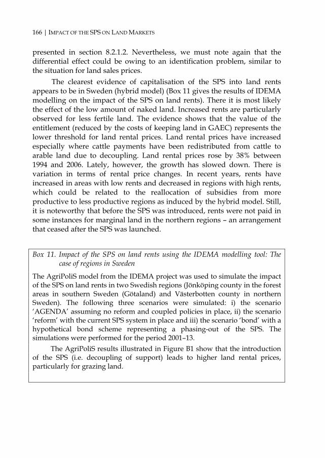
166 | IMPACT OF THE SPS ON LAND MARKETS
presented in section 8.2.1.2. Nevertheless, we must note again that the differential effect could be owing to an identification problem, similar to the situation for land sales prices.
The clearest evidence of capitalisation of the SPS into land rents appears to be in Sweden (hybrid model) (Box 11 gives the results of IDEMA modelling on the impact of the SPS on land rents). There it is most likely the effect of the low amount of naked land. Increased rents are particularly observed for less fertile land. The evidence shows that the value of the entitlement (reduced by the costs of keeping land in GAEC) represents the lower threshold for land rental prices. Land rental prices have increased especially where cattle payments have been redistributed from cattle to arable land due to decoupling. Land rental prices rose by 38% between 1994 and 2006. Lately, however, the growth has slowed down. There is variation in terms of rental price changes. In recent years, rents have increased in areas with low rents and decreased in regions with high rents, which could be related to the reallocation of subsidies from more productive to less productive regions as induced by the hybrid model. Still, it is noteworthy that before the SPS was introduced, rents were not paid in some instances for marginal land in the northern regions – an arrangement that ceased after the SPS was launched.
Box 11. Impact of the SPS on land rents using the IDEMA modelling tool: The case of regions in Sweden
The AgriPoliS model from the IDEMA project was used to simulate the impact of the SPS on land rents in two Swedish regions (Jönköping county in the forest areas in southern Sweden (Götaland) and Västerbotten county in northern Sweden). The following three scenarios were simulated: i) the scenario ‘AGENDA’ assuming no reform and coupled policies in place, ii) the scenario ‘reform’ with the current SPS system in place and iii) the scenario ‘bond’ with a hypothetical bond scheme representing a phasing-out of the SPS. The simulations were performed for the period 2001–13.
The AgriPoliS results illustrated in Figure B1 show that the introduction of the SPS (i.e. decoupling of support) leads to higher land rental prices, particularly for grazing land.

EU LAND MARKETS AND THE COMMON AGRICULTURAL POLICY | 167
Box 11. cont’d Figure B1. Simulated results for the Jönköping and Västerbotten regions in Sweden
(a) Average arable land rent, Jönköping
0
20
40
60
80
100
120
140
160
180
200
0 1 2 3 4 5 6 7 8 9 10 11 12
€/ha
AGENDA REFORM BOND
(c) Average grassland rent, Jönköping
0
20
40
60
80
100
120
140
160
180
200
0 1 2 3 4 5 6 7 8 9 10 11 12
€/ha
AGENDA REFORM BOND
(b) Average arable land rent, Västerbotten
0
20
40
60
80
100120
140
160
180
200
0 1 2 3 4 5 6 7 8 9 10 11 12
€/ha
AGENDA REFORM BOND
(d) Average grassland rent, Västerbotten
020
406080
100120140160
180200
0 1 2 3 4 5 6 7 8 9 10 11 12
€/ha
AGENDA REFORM BOND There are several reasons for this result. Profitability increases because
decoupling gives farmers more freedom in the choice of production structure and of whether to cultivate land. In addition, product prices at the European level are expected to increase with decoupling. Land rental prices also increase owing to the redistribution of cattle payments from cattle to land with the introduction of the SPS. Nevertheless, it should be noted that the impact of decoupling on land prices might not be as pronounced in other regions. In regions with favourable conditions for crop production, the introduction of the SPS does not influence farmers’ decisions on whether to cultivate land. The impact is also lower in regions with little livestock that had been eligible for direct payments before decoupling.
Phasing out the SPS would lead to reduced land rents. AgriPoliS results for many different regions indicate that land rents in many cases fall by 50% or even more in some regions, because SPS payments are capitalised into land prices and land rents. Apart from the lower land prices and land rents, the main effect of phasing out the SPS is that structural change in the agricultural sector would speed up considerably.

168 | IMPACT OF THE SPS ON LAND MARKETS
In Finland, when the SPS was introduced most of the rental contracts were renewed with the modification that entitlements return to the landowner when the rental contract expires. This adjustment to the contract does not affect the rent, which largely remains unchanged (see Box 12).
Box 12. Frictions between farmers and landowners over entitlement ownership in Finland
The ownership of entitlements in Finland has sparked significant media attention and intense discussion in the parliament as far back as 2002. A lot of uncertainty, extra work and fear accompanied the reform. Local officials underline that this reform instigated a great deal of concern (if not anger) among farmers and landowners and much effort has been expended to smooth things out.
The critical point in the public debate was who should obtain entitlements for land that was rented out at the time of SPS implementation. Based on FADN data, around 30% of land was rented in Finland in 2005.
Initially, based on the Finnish Act on the Implementation of the Single Payment Scheme, the SPS entitlement was granted for eligible hectares declared by farmers in 2006. A farmer is defined as a person who has a right of possession to land. Right of possession could be based on land ownership, leasing, inheritance or similar arrangements. This regulation essentially gave farmers the ownership rights to entitlements.
Nonetheless, the Committee of the Constitution in the Finnish parliament ruled that entitlements granted based on area under a rental contract concluded before 2006 should be transferred to landowners after termination of the rental contract. This ruling ensured the landowner’s rights to entitlements.
Thus, Finland currently finds itself in a situation in which national and EU legislation are in conflict. Despite this legal predicament, the common procedure is that the SPS entitlements are returned to the landowner after the expiration of the rental contract.
Presently, most of the entitlements are owned by landowners. Around 70% of entitlements were fixed to landowning farmers. The remaining 30% that had been linked to rented land and initially allocated to farmers were also returned to the landowners through the adjustment of rental contracts. Most of the rental contracts were renewed with the modification that entitlements return to the landowner when the rental contract expires (the adjustment does not affect the rent, which largely remains unchanged).

EU LAND MARKETS AND THE COMMON AGRICULTURAL POLICY | 169
In England (hybrid model), the regional flat-rate component of the SPS appears to tie the subsidy to the land, which is particularly evident in the rental value of land. The SPS appears to have put a floor on rental values. At the introduction of the SPS, on average 80% of the rental value was set by the CAP subsidy, whereas now on average only 50% of the rental value is attributable to the SPS, as land market participants have adjusted their behaviour and uncertainty behind the SPS has disappeared. In addition, the rise in land rents has reduced the contribution of the SPS to total rental prices. Simultaneously, non-farming landowners could also benefit from the SPS to a certain extent by applying directly for SPS entitlements themselves. This was especially the case for land that was under short-term rental contracts or share-farming arrangements, or used in the production of fruit, vegetables and potatoes.84
In Northern Ireland (hybrid model), it appears that landowners have obtained the regional component of the entitlement value (currently at €78 per entitlement against an average value of €355). Northern Ireland has an unusual rental system within the UK (conacre),85 in that virtually all rents 84 In England, a farmer who was in occupation of land in 2005 held the right to SPS entitlements whether (s)he was the landowner or tenant. Where there were short-term tenancies or licences (but for at least 10 months), the right to claim the SPS in 2005 in England could have belonged to either the landlord or tenant depending on the agreement. Short-term cropping leases (contracts) made it harder for landowners to claim the SPS. The contractor in contract-farming agreements had no right to land in a proper agreement, so entitlements were established by the landowner/farmer. Share-farming agreements were more difficult since only one person could claim the rights to the entitlements and meet the conditions.
Producers growing fruit, vegetables and potatoes were allowed to claim SPS entitlements despite not having received CAP support historically. They were broadly able to claim entitlements on the area they grew in 2003. But only a person responsible for growing these crops in 2003 (2004 or 2005 in some circumstances) would be eligible for claiming entitlements, which has led to some confusion and difficulties as the landowner may not have been the grower – meaning it may have been difficult for them to secure the entitlement claim. Defra later relaxed this rule so that landowners and growers could agree between themselves who was the ‘grower’ for the purpose of the entitlements. 85 Most of the rented area is leased through the conacre system in Northern Ireland, where land is let on a seasonal basis (nominally for 11 months or 364 days) without entering into a long-term commitment.
170 | IMPACT OF THE SPS ON LAND MARKETS
are for a period of less than a year; the entitlements stay with the landowner and not with the person renting the land. The SPS has also led to an adjustment of rents to accommodate the value of the regional component of the entitlements.86
In countries with the historical SPS model, the impact of the SPS appears to be significantly weaker. Only in a few countries is there evidence of some capitalisation of the SPS into land rents (e.g. Belgium and Italy).
Clearer evidence of partial SPS capitalisation into land rents under the historical model is found in Belgium. As outlined above (Box 10), the SPS is reinforcing the problem induced by a rigid rental market, which limits restructuring.
In Italy, there is some evidence of capitalisation of the SPS into land rents. The presence of the SPS has put upward pressure on the rental prices of eligible areas, leaving rent of ineligible areas unchanged. In the study region of Puglia, the SPS and farm size are the two main drivers that have contributed to rental price rises in recent years. More specifically, the trend towards the expansion of large farms has contributed to demand for rented land. This structural change combined with an imperfect entitlement market has slightly added to the growth in rental prices. Rental prices for land with entitlements are about 10-40% higher in comparison with land
86 In Northern Ireland, there was a problem with the conacre rental system when the SPS was first introduced. This was because thousands of farmers inadvertently claimed entitlements on the same field as their landlords. The introduction of a regional component (area reference amount) in the hybrid system encouraged landowners to submit claims for entitlements. Yet, because of the conacre system of short-term rents, many active producers also claimed on that land, without conferring with their landowners.
Additionally, there were cases in which landowners owned land but no livestock. In such cases, the person who owned the livestock received the payment under the historical system but the landowner was able to activate a payment under the area-based part (thus duplicate registration occurred). Some landowners own the area-based component of the SPS while farmers own the historical SPS component – this is not standard, but is largely owing to individual owners. If the landowner receives the historical SPS payment, (s)he receives an extra €78 compared with before. Land rents have already adjusted to consider this additional payment.

EU LAND MARKETS AND THE COMMON AGRICULTURAL POLICY | 171
not accompanied by entitlements. As explained earlier, this is not evidence of SPS capitalisation into land rents, but solely attributable to the price of the entitlements.
In the Netherlands, there is no evidence of the SPS affecting land rents. That being stated, non-farming landowners may gain access to the SPS entitlements through the regulatory system. A recent court ruling decided that after the expiration of a rental agreement, the SPS entitlements should be split in equal parts between the farmer and the landowner (see Box 13).
Box 13. Court ruling on the distribution of the SPS in the Netherlands
In a recent Dutch court case, the District Court of Zwolle decided that after the expiration of a rental agreement the SPS entitlements should be split into equal parts between the farmer and the landowner. The verdict was motivated by the judge comparing the entitlements to historical production quotas, for example those pertaining to milk or sugar beets. In doing so, the Court partially linked farm subsidies to land. The Dutch government and the national farmers association LTO are of the opinion that this was incorrect and they have encouraged the tenant to appeal to a higher court.
In Ireland, concerns were raised that the SPS would push up
agricultural rents. But the possibility to consolidate entitlements referred to earlier has offset this expected development. Since the introduction of the SPS, agricultural land rents in Ireland have not increased.
Also in France, there is no evidence of capitalisation of the SPS into land rents, because rental markets are strictly regulated in France. In Spain, the effect could not be identified due to missing data. In Greece, because of rigid rental markets the SPS does not affect land rents, which confirms the static effect of the SPS.
8.2.3 Who benefits from the SPS? This subsection summarises the effect of the SPS on land values and discusses the extent to which landowners benefit from the SPS.
First, in general the impact of the SPS on land markets is not substantial, although there is wide variation among countries. The

172 | IMPACT OF THE SPS ON LAND MARKETS
variation could be explained by the smaller number of countries that have implemented the hybrid model compared with the historical model.
Second, the evidence shows a larger impact of the SPS on land rents than on land sales prices. Yet this result is affected by the difficulty of isolating the effect of the SPS on land sales, because other factors have a greater influence on the sales market than the SPS.
Third, landowners tend to benefit more with the hybrid model than with the historical model. Landowners benefit more with the hybrid model through two channels: i) capitalisation of the SPS into land values (mostly driven by the low amount of naked land, which pushes up land values); and ii) specific implementation features of this model. With the hybrid model, the number of entitlements that farmers receive is equal to the total eligible area in the first year of SPS application. This aspect of the hybrid model has allowed some non-farming landowners to obtain entitlements in various ways, e.g. by cancelling the rental contract and applying themselves for entitlements, by adjusting rental contracts (to ensure that entitlements are returned to the landowner upon expiry) or other, similar arrangements.
Fourth, evidence shows that the historical model leads to low levels of SPS land capitalisation. Where this occurs, the drivers tend to be structural changes combined with constrained entitlement trading.
This observed low level of capitalisation of the SPS into land values with the historical model could be because it is more difficult to identify the effect in countries that have implemented this model. If the previous subsidy system was already capitalised into land values87 and the shift to the SPS had a marginal or no impact on land values, then both subsidy systems may have led to the same land capitalisation. But, parallel with the launch of the SPS was a significant rise in agricultural commodity prices. If the SPS is indeed not capitalised into land values, and the expected reduction in land values following SPS implementation has not occurred, then the unchanged prices after SPS implementation could just stem from the offsetting effect of higher commodity prices.
87 The literature estimating the impact of CAP subsidies on land values in the EU is almost non-existent. For this reason, it is hard to quantify their impact on land values.

EU LAND MARKETS AND THE COMMON AGRICULTURAL POLICY | 173
On the other hand, the hybrid model redistributed subsidies among farms, sectors and regions. This redistribution could explain why the impact of the SPS is easier to identify under this model, even though both models lead to the same capitalisation into land values. More specifically, the impact of the SPS is most visible in marginal, less fertile lands where other drivers are less relevant. The hybrid model tends to redistribute subsidies in favour of less productive lands, as the previous subsidies were highly correlated with productivity.
Table 17 summarises the landowner’s benefits from the SPS in the EUSCs, based on the analysis provided in this section. Landowners tend to benefit most from the SPS in Finland and Sweden and least in Greece and Ireland.88 In the rest of the countries examined, landowners’ benefits from the SPS are in the low to medium range.
Still, whether the SPS is channelled outside agriculture depends on whether landowners are farmers.89 Figure 31 shows the share of land renting in the UAA in EU member states in 2005. The prevalence of land renting varies significantly among EU countries. Comparing countries covered by this study, land rentals are highest in Belgium, France and Germany (more than 70% of the land used). In Sweden, farms rent approximately 50% of the land used. In Ireland, land renting is the lowest in the EU (17%). In the rest of the EUSCs, farms rent between 34% and 43% of the land used.90
These rental shares imply that in Belgium, Germany, Northern Ireland and Sweden, a major proportion of the SPS benefits could be
88 Land values were not significantly affected by the introduction of the SPS in Scotland. Since owner-occupancy in Scotland is around 70%, the benefit lies with the producer because of its historical nature. As such, landowners who are not actively involved in production do not benefit. 89 The effect of the SPS on the rural economy in general is contingent upon whether landowners live in rural or urban areas. As consistent data are not available, we are unable to address this issue. 90 In England, Northern Ireland and Scotland, land renting represented respectively 36%, 69% and 30% of the UAA in 2007.

174 | IMPACT OF THE SPS ON LAND MARKETS
channelled to non-farming landowners.91 This finding also holds for England and Finland, but to a lesser extent because farms rent around 30-36% of land. In addition, in some cases non-faming landowners enter farming to benefit from the SPS. This tendency is especially clear in Sweden, where some landowners who did not farm prior to the introduction of the SPS began doing so when the SPS was launched. In the rest of the countries, fewer SPS benefits will go to non-farming landowners because either land renting is less prevalent or SPS land capitalisation is small (or both). In these countries, farmers gain the largest proportion of the SPS.
8.3 Effects of the SPS on structural change This section analyses the effect of the SPS on structural change in agriculture. Among other things, structural change may be caused by alterations to productivity induced by technological or institutional innovations, or by the presence of imperfect rural credit markets. The SPS itself may reduce farm credit constraints and thereby increase productivity (see Ciaian and Swinnen, 2009). Adjustments in these areas can lead to the reallocation of land and farm exit and entry. Meanwhile, the decoupling introduced with the SPS may also have stimulated structural change in agriculture.
Based on the theoretical results presented in chapter 2 and appendix 2, if entitlements are fully tradable, then the SPS has no affect on structural change in agriculture – neither hampering nor inducing it. Structural change may be constrained by the SPS if entitlements are not fully tradable. In this instance, the SPS restricts land transactions and the reallocation of land from less productive to more productive farms. For example, with constrained entitlement trading, farmers in decline are less willing to reallocate land as they lose benefits from the SPS. If the SPS affects farms’ credit, the SPS directly induces change in agriculture. More farm credit stimulates investments and input use, which enhance productivity and boost land transactions (Ciaian and Swinnen, 2009).
91 This may not be the case in situations where a farmer rents land from another farmer rather than from a non-farming landowner, as for example in Northern Ireland.

EU LAND MARKETS AND THE COMMON AGRICULTURAL POLICY | 175
Next, we consider the evidence on the effect of the SPS on structural change in agriculture based on country studies. Structural change is a long-term process. For this reason, it may be too early to assess the developments observed in the few years available since the start of SPS implementation. Furthermore, substantial other structural change unrelated to the SPS has occurred in agriculture in the last few years. In particular, there has been a sharp increase in agricultural output and input prices and expansion of bio-energy production. Together, these factors make it difficult to isolate the impact of the SPS on structural change in agriculture in the study countries and regions.
The decoupling of previous subsidies with the introduction of the SPS was identified in most country studies as the factor most likely to have brought about structural change in agriculture. Decoupling led to changes in production structures and input use, and to a certain extent, it provoked farm exit. With the SPS, farmers’ decisions have predominantly been driven by market incentives, while previously they took into account direct payments.
The SPS has a notable effect on farm exits. More specifically, evidence from several country studies (e.g. Belgium, Finland, Ireland, Sweden and the UK) indicates that the SPS may constrain farm exit. This effect of the SPS works in combination with the imperfect tradability of entitlements. With the presence of imperfect tradability, entitlement prices are depressed, thereby reducing the advantages of selling them. This reduces farmers’ incentives to exit, which in turn diminishes the likelihood of land reallocation (because SPS benefits necessitate land to activate them). Farmers in this situation tend to have little opportunity for off-farm benefits or these are lower relative to the SPS.
One of the strategies of farmers considering exit is a shift from full- to part-time farming (e.g. Belgium, Germany and Italy). This inclination appears to be more common in marginal areas. To obtain SPS payments, it is not necessary to produce, but land must be kept in GAEC. Part-time farming allows farmers who would otherwise exit to trim down unprofitable farm activities, while ensuring that they continue to benefit from the SPS.
In Belgium, the practice is that farmers rent out their plots, with some selling land after exiting. As a result of the SPS, exiting older farmers remain on their farms longer, often hiring labour to maintain their land in GAEC.

176 | IMPACT OF THE SPS ON LAND MARKETS
In Greece, the SPS tends to be an incentive for the rural population (and especially new farmers) to stay in the countryside, as farmers can receive the payments with minimal obligations.
In Germany, the evidence shows that the SPS affects the decision on whether a farm is operated on a full- or part-time basis. There was a significant increase in the number of part-time farmers in Germany in the period 2005–07 (Figure 32). There are two possible explanations. The first is that small businesses or hobby farms that did not apply for CAP payments before the introduction of the SPS, began to operate as part-time farms to facilitate applying for the SPS. The second explanation is that full-time farmers extended their land use to the meet minimum requirements and thus possibly switched to part-time farming on their entire holding. Because the area share has remained constant or even declined, the first line of reasoning seems more likely. This result is confirmed by the expert surveys in the case study regions.
Furthermore, it is expected that structural changes in marginal grassland regions (e.g. mountain pastures) will be decelerated in Germany owing to the increasing entitlement payments in these regions induced by the gradual shift from the hybrid model to the regional one (i.e. Bavaria).
In the UK, the exit decisions of many farmers appear to have been delayed until 2012, as they know the SPS will run at least until then.
The impact of the SPS on hired labour is small. There is insufficient evidence to be able to identify patterns of SPS effects on agricultural labour developments.
The hybrid model has had some impact on land rental markets. More precisely, it has stimulated farm entry and engendered uncertainty in rental markets. This development has been observed in all countries with the hybrid model (except Germany), while it has not been observed in any country implementing the historical model. With the hybrid model, the allocation of entitlements is based on current land use (i.e. land use at the time the SPS was introduced) and not on the land use in the reference period. This policy stimulated farm entry because non-farming landowners had the possibility to obtain entitlements if they had land at their disposal when the SPS was introduced. Non-farming landowners just need to obtain land back from the tenant. It has been common for landowners to cancel rental contracts, enter into short-term contracts, or just before the SPS was launched, not renew expiring contracts. This ensured that non-farming landowners could apply for entitlements themselves at the time the SPS

EU LAND MARKETS AND THE COMMON AGRICULTURAL POLICY | 177
was introduced. There is some evidence, especially in Sweden, that landowners entered farming (especially those with low non-farming opportunity costs) just to obtain entitlements. This trend exacerbates uncertainty, however, and hampers farm decision-making on the part of tenant farmers.
In countries that have implemented the historical SPS model, the number of entitlements farmers receive depends on the subsidies and the eligible area in the reference period (2000–02). For this reason, the only owners of entitlements could be individuals who were farmers in the reference period and who received subsidies. This stipulation reduces the possibility for non-farming landowners to obtain entitlements.
The effect of the SPS on farm credit The SPS has had a crucial impact on rural credit markets. Credit market imperfections are important for the rural economy (e.g. Blancard et al., 2006; Färe et al., 1990). The main factors leading to credit constraints are missing markets, asymmetric information and incentive problems. Particularly in agriculture, credit problems arise for a variety of reasons:92 • There is a considerable time lag between the purchase of inputs and
the sale of production. • Farms are generally small. • Farms face a complex management environment (lengthy,
biologically-based production, complicated monitoring, a spatial dispersion of production, etc.).
• The value of farm collateral tends to be lower for the lender than for the farmer.
• Finally, the monitoring of farm activities is costly. The SPS may have substantial implications for farms’ access to credit
by alleviating credit constraints. If farms receive the subsidies at the beginning of the season, they can use the SPS directly to pay for inputs. If farms receive SPS payments at the end of the season, the SPS can also improve their access to credit, as the subsidies can be used as collateral for bank credit (see also Ciaian and Swinnen, 2009).
92 See Binswanger and Rosenzweig (1985) and Barry and Robison (2001).

178 | IMPACT OF THE SPS ON LAND MARKETS
The SPS is not expected to lead to a significant change in farms’ access to credit compared with the previous (coupled) subsidy system. The coupled subsidies introduced by the 1992 CAP reform and Agenda 2000 could also be used as collateral for obtaining bank credit or directly to finance farm inputs depending on the time when the coupled subsidies were received by farmers. There are some differences, however, explained by two main factors. First, when used as collateral for bank credit, the SPS and the previous subsidy system may pose differing risks for lenders. For example, animal payments were granted per head of animal. From the bank’s perspective, this creates some uncertainty, as the payments depended on the number of animals stocked and any damage to the stock (e.g. disease) may reduce the total payments. Under the SPS, if farms do not respect cross-compliance criteria, this may lead to lower SPS payments. This possibility creates specific uncertainty for banks and may reduce their willingness to provide farm credit. Second, the hybrid model has redistributed subsidies among farms, which in turn has affected access to credit. Pre-financing ability or access to credit has been reduced for those farms that receive fewer subsidies under the SPS than under the previous subsidy system. Conversely, farms that receive more subsidies under the SPS compared with the previous system have gained improved access to credit.
Several country studies confirm that the SPS affects farms’ access to credit (e.g. France, Germany, Italy and Spain). The SPS increases farm income and hence alleviates farm credit constraints in a straightforward way. In addition, the SPS is seen to increase access to short-term credit from banks by use as collateral. Because of the uncertainty about the future of the SPS, it appears that the SPS does not have an impact on long-term credit. Lenders are not willing to provide long-term credit by accepting future SPS payments as collateral.
In Germany, it is common practice for farms that activate the subsidy payments to receive short-term credit – which has not altered with the introduction of the SPS.93
93 One expert interviewed in Saxony even responded that the SPS might have negative effects on creditworthiness: because of cross-compliance controls, SPS payments are more risky.

EU LAND MARKETS AND THE COMMON AGRICULTURAL POLICY | 179
Similarly, in Italy, the SPS helps farmers to finance farming activities and obtain credit. There is a trend towards the expansion of large farms and the abandonment of small ones in Italy. The SPS may have slightly encouraged this tendency, although the actual impact is unclear. The increase in liquidity and easier access to credit by farmers owning large amounts of entitlements may have been a contributing factor.
In France, the SPS is paid later in the year compared with pre-reform direct payments. For this reason, farmers may need more short-term loans from banks with the SPS compared with the previous subsidy system. Moreover, the SPS does not represent better credit collateral than pre-reform direct payments because of its uncertain future.
In Spain, there is no great difference between the SPS and the previous subsidy system in terms of farms’ access to credit. The only notable difference is the higher risk farmers may pose because of cross-compliance controls and possible reductions of payments if these requirements are not respected. Yet, in some regions, e.g. in the Valencian Community, where the SPS is paid at the end of the season, farmers have to rely on credit to finance their costs until they receive the SPS payment. In this situation, farms use the commitment of the regional ministry of agriculture to pay out the SPS as the collateral for credit.
8.4 Influence of changes in the SPS models on land values In this section, we analyse the impact of a hypothetical policy change. We assume that the current SPS models used by the EUSCs are replaced by a regional model. We focus on how the level of payments, the share of naked land and the link between payments and land affect the capitalisation of the SPS into land values. The analysis in this section is based on the analysis and findings from the previous chapters.
None of the countries investigated in this study initially implemented a purely regional model. Most of the countries selected the historical model. Northern Ireland and Sweden chose the static hybrid model, while Finland, Germany and England opted for the dynamic hybrid model, which is gradually being replaced by the regional model. The complete switch to the regional model will occur in 2016 in Finland, in 2013 in Germany and in 2012 in England (Table 8).
The chief characteristic of the regional model is that it equalises the value of all entitlements. In a given region, all farms receive entitlements with the same value. The effects of the shift to the regional model will be

180 | IMPACT OF THE SPS ON LAND MARKETS
determined by three key features: i) whether new entitlements are allocated, ii) the redistribution of subsidies among regions and iii) how landowners are treated with respect to access to the entitlements.
The insights from the previous chapters suggest that a switch to the regional model may have consequences for land markets. The most important potential effects can be summarised as follows: • The evidence found in this study indicates that the SPS leads to at
least some land capitalisation with both the hybrid and historical models. As a result, a shift to the regional model may lead to changes in the relative land prices among regions. This stems from the regional model redistributing subsidies among regions, which leads to higher prices in less productive regions and lower prices in more productive ones.
• The effects are expected to be larger in those regions that currently apply the historical model, because they have already materialised to a certain extent in countries that use the hybrid model. Note that under the hybrid model, a share of payments has already been redistributed. In these countries, the policy shift to the regional model will reinforce this redistribution even further.
• Whether the shift to a regional model will lead to more widespread land capitalisation of the SPS compared with the current SPS models will depend on the implementation details of the regional model. Such details include, for example, whether the number of entitlements will increase or stay at the present level and the extent to which non-farming landowners’ access to entitlements will be regulated and enforced. Evidence from this study suggests that landowners tend to benefit more with the hybrid model than with the historical model for two reasons: i) more entitlements were allocated under the hybrid model and ii) the implementation features of the hybrid model allowed landowners to obtain entitlements or to ‘force’ farmers to return entitlements to them when rental contracts expired.
• Yet, if the total number of entitlements allocated is not affected by the policy changes (only the entitlement value is equalised), the upward pressure on land prices will continue to be stronger in countries that currently use the hybrid model. This is because in these countries there is less naked land than in countries using the historical model.
• Frictions between farmers and landowners are expected to increase with the shift to the regional model. Again, this will be heavily

EU LAND MARKETS AND THE COMMON AGRICULTURAL POLICY | 181
influenced by the implementation details of the regional model. If additional entitlements are allocated along with the policy shift, non-farming landowners will be able to keep the entitlements, as has been observed in the EUSCs that apply the hybrid model. This is mainly because under the hybrid (or regional) model, the number of entitlements that each farm receives depends on the amount of eligible area when the SPS was introduced. In contrast, under the historical model it depends on the amount of land that generated support in the reference period. Hence, the key factors that will determine whether frictions between farmers and landowners intensify with the policy shift are the extent to which the access to entitlements of non-farming landowners is regulated and enforced, and the extent to which the number of newly allocated entitlements (if any) is based on current or past land use.
• The impact of the policy shift on land markets, especially on the capitalisation into land values, is contingent upon the clarity and transparency of the implementation process. If the shift creates uncertainty among farmers, this will affect land markets. More precisely, it will constrain entitlement markets – which in combination with the structural changes taking place in the agricultural sector, may enhance land capitalisation.
• In summary, uncertainty and the implementation specifics of the policy change will affect the entitlement market, which in turn will determine the capitalisation of the SPS into land values. For example, there is evidence from the Netherlands that the expected shift to the regional model in the future affects the trade in high-value entitlements. This expectation reduces the market price of high-value entitlements, as market participants believe that a shift to the regional model will likely cut the value of such entitlements. On the other hand, there is evidence from Belgium that the trade in low-value entitlements has been stimulated by the regulation that allows young farmers to replace low-value entitlements with those of higher value equal to the regional average.
• Still, the shift to the regional model will increase transparency in the entitlement market, as all entitlements will have the same value. Above all, it will stimulate transactions on the entitlement market and thus lead to lower capitalisation of the SPS.

182 |
9. GENERAL CONCLUSIONS
ur conclusions are organised under three themes: land markets in the EU study countries, CAP reform and its impact on land markets, and data limitations. In the section on land markets in the
EUSCs, we summarise the main findings about the nature of the land markets, their development and the key drivers of land values. In the section on CAP reform and land markets, we discuss the principal findings on the effects of SPS implementation, the activation of entitlements along with their valuation and trade, the distribution of SPS benefits and the ramifications for structural change. In the final section, we outline the chief limitations of the present research.
9.1 Land markets in the EU study countries
9.1.1 Nature and developments The amount of rented land and the volumes of rental transactions differ greatly among the EUSCs. Farms in Belgium, France, Northern Ireland and Germany are more likely to rent land (more than 65% of the land used). In Sweden, farms rent approximately 50% of the agricultural land used. In contrast, the prevalence of land renting is lowest (17%) in Ireland. In the rest of the countries covered by this study, farms rent between 34% and 43% of the land used. The share of rented farmland of the total UAA is increasing in most of the EUSCs.
Agricultural land prices also vary widely across the EUSCs. In the peak years, differentials between the most and least expensive countries exceeded 2,000% – ranging from around €2,000/ha in parts of Sweden to over €40,000/ha in parts of the Netherlands. These figures imply that awarding the same amount of subsidy per hectare of agricultural land would have quite diverse impacts on land prices.
O

EU LAND MARKETS AND THE COMMON AGRICULTURAL POLICY | 183
The variation in rental prices is somewhat lower than in sales prices but large differences are likewise apparent. The difference in rental prices between the lowest and highest countries was around 600% in 1992 and over 700% in 2006.
Changes in agricultural land prices over the past decade have been diverse as well. Over the period from 1992 to the present, real farmland sales prices have decreased by around 25% in Greece, while increasing by around 250% in Ireland. Developments in rental prices since 1992 have ranged from a decline of around 25% in Finland to a rise of around 55% in Spain.
This cross-country heterogeneity in agricultural land markets suggests that farmers and landowners in these different land markets may be affected by (changes in) the CAP in alternate ways.
9.1.2 Drivers of land values Agricultural commodity prices and productivity, infrastructural expansion and urban pressures have marked influences on land markets, but their relative importance differs for rental and sales markets. First, agricultural commodity prices and productivity are significant drivers of agricultural land prices, but their effects seem to be more striking for rental markets than for sales markets. Second, urban pressures – such as growing housing demand – have pronounced effects on agricultural land prices, especially in densely populated EUSCs (e.g. Belgium and the Netherlands) and faster growing economies (e.g. Ireland and Spain). The same applies to the role of infrastructural expansion in driving up land prices. The latter two factors in particular influence sales prices.
Land market regulations affect land prices and exchanges – especially land rentals. Rental prices for agricultural land tend to be more regulated by governments than sales prices. In one-third of the EUSCs, the maximum rental prices are set by the government.
The duration of rental contracts is regulated in some of the EUSCs, which influences the responsiveness of the rental market to agricultural policy changes. The length of rental contracts is regulated by the government in Belgium and France (with a contract duration of nine years minimum), the Netherlands (six years minimum) and Spain (five years minimum). In several EUSCs (e.g. France), the renewal/inheritance of rental contracts is also regulated. In these countries, formal rental markets are stickier and the time lag is longer in adjusting to policy changes. The prevalence of land renting is typically higher in countries with strict rental market regulations,

184 | GENERAL CONCLUSIONS
such as Belgium and France. These two countries have the highest minimum lengths of rental contracts (nine years) and the highest shares of rented area (77% and 75% in 2006, respectively) among all the EUSCs.
Land taxes differ significantly across the EUSCs. Three kinds of tax regulations that affect market participants’ decisions to buy, own or sell agricultural land have been studied: sales taxes, purchase taxes and ownership taxes. Tax rates for land transactions are heterogeneous across the EUSCs, spanning from 1% for low-value land in the UK to 18% for high-value farmland in Italy. The same applies to ownership taxes, ranging from a 0% tax rate on farmland in Finland to over 15% in the southern EU countries.
Neither low taxes for farmland ownership and transactions nor entitlements constrain structural change, but they do expose farmland to non-agricultural investors. Low transaction taxes for farmland and SPS entitlements facilitate structural change through the reallocation of agricultural land and entitlements from less productive to more productive farms (e.g. Germany). On the other hand, agricultural land markets in countries with low transaction taxes are more exposed to speculative farmland purchases (and sales) by non-agricultural investors (e.g. Finland). Differentiated farmland ownership taxes for farmers and non-farmers reduce the incentives for long-term, speculative farmland purchases (and sales) by non-agricultural investors, but hinder structural change (e.g. Greece).
CAP subsidies have an impact on land values, but the impact varies substantially across countries and appears relatively modest compared with other factors, especially where land prices are high. CAP subsidies appear to affect land sales prices in the EUSCs. Still, their relative importance seems limited compared with other drivers. Generally, the lower the land price, the higher is the impact of CAP policies in this respect (e.g. in the Nordic regions in Finland and Sweden). In countries such as the Netherlands and Ireland, where land prices are very high or are rapidly increasing, factors other than CAP policies appear to have a greater bearing.
9.2 CAP reform and land markets
9.2.1 Implementation of the SPS The EU member states could choose among three SPS implementation models: the historical, regional and hybrid model. Under the historical model, the SPS payment is farm-specific and equals the support the farm

EU LAND MARKETS AND THE COMMON AGRICULTURAL POLICY | 185
received in the reference period. This is the most common SPS model in the EUSCs. Under the regional model, an equal per-hectare payment is granted to all farms in the region.
Concerns about the redistribution of subsidies were by far the most compelling factor for the EUSCs that selected the historical SPS model over the regional one. A major motivation for England, Finland and Germany in deciding to apply the dynamic hybrid model instead of directly implementing the regional one was to smooth the adjustment of the farming sector over time. In all cases, receipt of the full SPS support is conditioned on the fulfilment of cross-compliance requirements. More precisely, a farmer receiving SPS support must respect SMRs and maintain land in GAEC.
None of the EUSCs implemented the purely regional model. The comparative insights are therefore based on contrasting the implications of the historical model with the hybrid model.
9.2.2 Entitlements: Activation, trade and valuation The share of non-activated entitlements of the total distributed entitlements is low. For most EUSCs, it is less than 3%. The value of non-activated entitlements tends to be lower than the value of activated ones. Non-activated entitlements mainly stem from the absence of eligible area and administrative burdens.
The share of activated entitlements tends to be somewhat higher in countries using the hybrid model than in those using the historical one. We find that this might be owing to specific criteria relating to the implementation of the hybrid model.
There is a wide variation in the face value of entitlements among and within the EUSCs. This variation seems to be determined by the commodity structure, the level of support provided in the reference period, the SPS model applied and implementation details.
There are large differences among the EUSCs in the restrictions on trading entitlements. EU regulations allow entitlements to be tradable but certain constraints are imposed by the EU. Member states have some flexibility in introducing additional country-specific limitations on entitlement tradability. Spain, Italy and France have the tightest restrictions on entitlement trading.

186 | GENERAL CONCLUSIONS
The trade of entitlements is most often conducted directly among farmers, although sometimes market agents or farm organisations play a role. Spain appears to have the most developed entitlement trading system, similar to an auction.
There is no informal trading in entitlements, except among family members. An informal entitlement market was not found in any of the EUSCs, because in order to receive payments, entitlement holders need to be identifiable. Unofficial ‘trade’ may occur among members of the same family, however.
The entitlement market tends to be smaller in regions under the hybrid model compared with the historical model. Under the historical model, trade is likely to be driven by structural change – because the SPS was implemented in 2005–07, but the SPS entitlements were distributed based on land use in 2000–02. With the hybrid model, entitlement trading is driven by a combination of decoupling and the fact that relatively more entitlements were allocated than with the historical model. Structural change is less of an influential factor in the entitlement market under the hybrid model, as entitlements were distributed based on the area used in the first year of the SPS application. Differences in the implementation features of the two SPS models may explain the higher volume of trade with the historical model than with the hybrid one. This is chiefly evident in the short run, which is investigated in this study.
Preliminary evidence suggests that the trade in entitlements is also affected by the functioning of land markets, restrictions on the tradability of entitlements, the availability of an opportunity to consolidate entitlements and the amount of naked land.
Entitlements are most often traded with land. Evidence from the EUSCs shows that with few exceptions, entitlement trades are usually accompanied by land.
Our data show that the market price for entitlements in most EUSCs is between one and three times the annual face value of the entitlement. A simple calculation would indicate that with perfect markets and without uncertainty, the entitlement price would be in the range of four to five times the face value if the SPS were to run until 2013 or in the range of ten to twenty if the SPS were to run indefinitely.
Several factors may explain the observed gap in the entitlement price between theoretical expectations and empirical evidence: i) uncertainty about the future of the SPS (e.g. modulation and the health check), ii) the

EU LAND MARKETS AND THE COMMON AGRICULTURAL POLICY | 187
additional costs of the SPS (e.g. administrative costs), iii) the taxes and fees imposed on transactions and iv) credit market imperfections. The low market price of the entitlements may also reflect the capitalisation of the SPS into farmland values.
9.2.3 Effects of SPS implementation Our theoretical framework and empirical evidence in the literature suggest that the impact of the SPS on land markets depends on several factors, including the SPS model applied and specific implementation features, market imperfections, transaction costs, market structure and other policies.
On average, the impact on land markets of the switch to the SPS appears to have been weak and it has not led to lower capitalisation than under coupled policies, although there has been variation among the EUSCs and regions. Preliminary evidence presented in this study indicates that on average the impact has been limited. We do not observe major declines in land prices with the shift to decoupled policies, which implies that there are no significant reductions in the capitalisation of support.
The introduction of the SPS appears to have had a larger impact on land rents than on farmland sales prices. The net effect on land values also depends on the rate of SPS capitalisation into land values and on the relative significance of the SPS compared with other drivers of land values. The empirical evidence from this study implies that the relative weight of the SPS in determining farmland prices against that of other drivers of land values is higher for rents than for sales prices.
Preliminary evidence reveals that the historical model leads to lower capitalisation of the SPS into land values than the regional or hybrid models. In countries with the hybrid model, capitalisation appears to be driven by the low amount of naked land. In countries with the historical model, the impact of the SPS appears to be substantially weaker. Where SPS land capitalisation occurs, the most influential factor tends to be structural change combined with constrained entitlement trading (most notably in Belgium). In countries such as Greece, there is little activity on the land market and hence there is little capitalisation of the SPS. In Ireland, the possibility to consolidate entitlements has reduced the pressure of the SPS on land markets and SPS land capitalisation seems to be minimal.
We also find that instead of reducing capitalisation, introduction of the SPS appears to have increased capitalisation in the least productive countries. The SPS seems to have put a floor on land values in less productive regions (e.g. in

188 | GENERAL CONCLUSIONS
Sweden and parts of the UK). The clearest evidence of the influence of the SPS on land values is higher land values for less fertile land (e.g. grassland). But this finding could also be rooted in the redistribution that came with the hybrid model.
In countries with regulated rental prices, implementation of the SPS seems mainly to affect unofficial markets. In these member states, there is little effect on official prices (since these are regulated), but where regulations lead to the existence of unofficial markets for agricultural land, the SPS tends to increase both rental prices (e.g. Belgium) and volumes on the unofficial market (e.g. Belgium and the Netherlands).
9.2.4 Distribution of the SPS benefits Landowners tend to benefit more from the hybrid model than from the historical model. More specifically, landowners benefit more under the hybrid model through two channels. The first is the capitalisation of the SPS into land values. This is mostly the case where low amounts of naked land drive up land values. The second channel concerns the implementation features of the hybrid model. Under the hybrid model, the number of entitlements that farmers receive is equal to the total eligible area in the first year of the SPS application. This has enabled some non-farming landowners to obtain entitlements either by cancelling the existing rental contracts and applying for entitlements themselves or by adjusting rental contracts to ensure that entitlements return to them after the contract expires, or by undertaking other similar arrangements.
The distribution of the SPS payments to landowners appears to differ markedly among the EUSCs. From our country studies, it seems that landowners benefit most from the SPS in Finland and Sweden (60-100% of the value of the entitlement) and least in Greece and Ireland (0-10%). In the rest of the countries, the benefits that accrue to landowners from the SPS are in the low to medium range (10-60%).
The distribution of the SPS additionally depends on whether landowners are also farmers, which varies among the EUSCs. As mentioned above, the prevalence of renting land differs greatly among the EUSCs. The evidence in this study suggests that in Germany, Northern Ireland and Sweden, a substantial share of SPS benefits will be channelled to non-farming landowners. This finding also holds (but to a lesser extent) for England, Finland and Scotland. In the rest of the EUSCs, a lower share of the SPS will go to non-farming landowners, either because renting land is less common

EU LAND MARKETS AND THE COMMON AGRICULTURAL POLICY | 189
or because there is little capitalisation of the SPS into land values (or both). In these countries, farmers appear to gain the largest proportion of the SPS.
9.2.5 Effects on structural change It is too early to observe significant effects of the SPS on structural change in agriculture. Structural change is a long-term process, and it is therefore premature to assess the developments observed one or two years since the SPS was introduced. Meanwhile, substantial structural changes related to factors other than the SPS have occurred in agriculture in the last few years. Still, the decoupling of subsidies with the introduction of the SPS has been identified by most country studies as having had a major impact on structural change in agriculture.
The SPS seems to constrain farm exit and increase part-time farming. Evidence from several countries, e.g. Belgium, Finland, Sweden and the UK, suggests that the SPS constrains farm exit. The SPS also appears to increase part-time farming – an effect that seems more pronounced in marginal areas. Part-time farming allows farmers to reduce unprofitable farm activities while still benefiting from the SPS. No significant difference can be identified between the hybrid and historical models in this respect.
The impact of the SPS on hired labour appears small. There is insufficient evidence to identify the effects of the SPS on other agricultural labour developments.
The hybrid model has stimulated (formal) farm entry, unlike the historical model, although it has also given rise to uncertainty on the rental markets. This is because under the hybrid model, the allocation of entitlements is based on land use when the SPS was introduced and not on land use in the reference period. We find some evidence that landowners have started farming in order to gain access to the entitlements. The long-term net impact of these rent-seeking activities on farm structures is unclear. Nevertheless, it has affected the distribution of SPS rents and the market in entitlements in ways that are different from the historical model, where such activities do not appear to have occurred.
The introduction of the SPS has reduced farm credit constraints, especially for short-term credit. An interesting and potentially significant side effect of the SPS has emerged in rural credit markets. Several country studies (e.g. France, Germany, Italy and Spain) confirm that the SPS affects farms’ access to credit. If farms receive the subsidies at the beginning of the season, they can use the SPS to pay for inputs directly. If farms receive SPS

190 | GENERAL CONCLUSIONS
payments at the end of the season, the SPS subsidies can be used as collateral for bank credit. Because of uncertainty about the future of the SPS, however, it appears that the SPS has no influence on long-term credit. Lenders are not willing to provide longer-term loans by accepting future SPS payments as collateral.
9.2.6 Effects of changes in the SPS model on land values None of the EUSCs implemented a purely regional model. Most of the EUSCs have applied the historical model and some the dynamic hybrid model, which will gradually be replaced by the regional model.
The key characteristic of the regional model is that it equalises the face value of all entitlements. The effect of the shift to the regional model will be determined by three critical features: i) whether new entitlements are allocated, ii) the redistribution of subsidies among regions and iii) how landowners are treated with respect to access to the entitlements.
The regional model may lead to changes in relative land prices among regions. The regional model redistributes subsidies among regions, which is expected to lead to higher prices in less productive regions and lower prices in more productive ones. The effect is expected to be more marked in those regions currently applying the historical model. Under the hybrid model, a share of the payments has already been redistributed.
The implementation details of the regional model will largely determine whether the shift to the regional model will increase the capitalisation of the SPS compared with current SPS models. Among other things, this will depend on whether the number of entitlements increase or stay at the present level and how much non-farming landowners’ access to entitlements is regulated and the rules enforced.
Yet if the total number of entitlements allocated is affected by the policy changes, the upward pressure on land prices will continue to be stronger in those countries that have implemented the hybrid model.
Frictions between farmers and landowners are expected to intensify with the shift to the regional model. The chief factors in this regard will be the extent to which the access to entitlements of non-farming landowners is regulated and enforced, and the extent to which newly allocated entitlements (if any) are based on current or past land use.
The change in models may have an impact on the levels of uncertainty and transparency in the entitlement market. If the shift to the regional model provokes uncertainty among farmers, it will constrain entitlement markets
EU LAND MARKETS AND THE COMMON AGRICULTURAL POLICY | 191
and may induce more land capitalisation. On the other hand, the shift to the regional model may increase transparency in the entitlement market, as all entitlements will have the same face value.
9.3 Limitations The results reported in the present study are subject to certain limitations. First, as in any empirical analysis, one should keep in mind data limitations when interpreting the results. In particular, data on land transactions are scarce for the period after the SPS was implemented. The rather short time span since the implementation of the SPS combined with the varying quality of the available data has not allowed us to perform a consistent econometric analysis. In addition, farmland markets are only marginally covered in national statistical data. For example, in several countries uniform databases for the land market are still to be established (e.g. the land cadastre in Greece).
Second, the global food markets have simultaneously undergone major changes, such as a rise in world prices for agricultural commodities. Rising energy prices have increased competition for farmland from the bio-energy sector. These factors reduce the ability to isolate the impact of the SPS on agricultural land markets.
Third, the qualitative analysis performed in the present study does not enable us to assess confidence intervals nor does it allow us to perform sensitivity analysis on the results or checks on statistical robustness. Although we have attempted to systematically verify all the input data and prove our findings using several alternative sources of information, this cannot replace statistical robustness checks. This is a promising avenue for future work, when more and better quality data become available.
Fourth, the results for farmland sales prices are not directly comparable with the results for farmland rental prices. On the one hand, it is rather difficult to identify the impact of the SPS on land sales prices, because these are more strongly driven by non-agricultural factors and market expectations are more important. For land rents, this problem is less acute. On the other hand, rental markets for agricultural land are more regulated than sales markets are and in rigid markets, the contracts tend to be of a longer duration. Rental contract regulations may delay or mitigate the capitalisation of the SPS into higher land rents than observed in rental market data.

192 | GENERAL CONCLUSIONS
Moreover, if the previous area payments introduced under the 1992 CAP reform and under Agenda 2000 were already capitalised into land values, then the capitalisation of the SPS may be difficult to observe because of biased counterfactual data. The empirical literature estimating the impact of previous subsidies on land values is scarce but it tends to find that the previous area payments have had an affect on land values (Duvivier et al., 2005; Patton et al., 2008). This finding implies that the SPS may be capitalised into land values even where land prices remain stable after the introduction of the SPS. Yet, to be able to quantify the precise rate of SPS capitalisation, other factors that may influence land values also need to be taken into account along with the previous area payments. Further work is needed on these aspects, to determine the unbiased effect of the SPS.
| 193
BIBLIOGRAPHY
Abler, D. (2001), “Elasticities of Substitution and Factor Supply Elasticities in Canadian, Mexican and United States Agriculture: A Review of Past Studies”, OECD Market Effects of Crop Support Measures, OECD, Paris, pp. 57-88.
Alliance Environnement (2007), Evaluation of the Application of Cross-compliance as Foreseen under Regulation 1782/2003, Study prepared for DG Agriculture, Alliance Environnement, Groupement Européen d”Intérêt Economique (retrieved from http://ec.europa.eu/ agriculture/eval/reports/cross_compliance/index_en.htm).
Alston, J.M. (2007), “Benefits and Beneficiaries from US Farm Subsidies”, The 2007 Farm Bill and Beyond, AEI Agricultural Policy Series, American Enterprise Institute (retrieved from http://www.aei.org/ farmbill).
Alston, J.M. and J.S. James (2002), “The Incidence of Agricultural Policy”, in B.L. Gardner and G.C. Rausser (eds), Handbook of Agricultural Economics, Vol. 2B, Amsterdam: Elsevier, pp. 1689-1749.
Balmann, A. (1999), “Path Dependence and the Structural Development of Family Farm Dominated Regions”, paper presented at the “IX European Conference of Agricultural Economists”, Warsaw, 24-28 August.
Barnard, C.H., R. Nehring, J. Ryan and R. Collender (2001), “Higher Cropland Value from Farm Program Payments: Who Gains?”, Agricultural Outlook, Special Edition, November, pp. 26-30.
Barnard, C.H., G. Whittaker, D. Westenbarger and M. Ahearn (1997), “Evidence of capitalisation of direct government payments into US cropland values”, American Journal of Agricultural Economics, Vol. 79, No. 5, pp. 1642-1650.
Barry, P.J. and L.J. Robinson (2001), “Agricultural Finance: Credit, Credit Constraints and Consequences”, in B.L. Gardner and G.C. Rausser, (eds), Handbook of Agricultural Economics, Amsterdam: Elsevier, pp. 513-571.

194 | BIBLIOGRAPHY
Bartolini, F., V. Gallerani, M. Raggi and D. Viaggi (2008), “Effectiveness of Cross-Compliance under Asymmetric Information and Differentiated Compliance Constraints”, paper presented at the XII EAAE Congress: “People, Food and Environments: Global trends and European Strategies“, Ghent (Belgium), 25-29 August.
Bayerisches Staatsministerium für Landwirtschaft und Forsten (BayStMLF) (2006), Bayerischer Agrarbericht 2006, BayStMLF, München.
Bierlen, R., L.D. Parsch, B.L. Dixon and B.L. Ahrendsen (2000), “The 1996 FAIR Act: Measuring the Impacts on Land Leasing”, Review of Agricultural Economics, Vol. 22, No. 2, pp. 336-354.
Binswanger, H. and M. Rosenzweig (1986), “Behavioral and Material Determinants of Production Relations in Agriculture”, Journal of Development Studies, Vol. 22, No. 3, pp. 503-39.
Blancard, S., J.P. Boussemart, W. Briec and K. Kerstens (2006), “Short- and Long-Run Credit Constraints in French Agriculture: A Directional Distance Function Framework Using Expenditure-Constrained Profit Functions”, American Journal of Agricultural Economics, Vol. 88, No. 2, pp. 351-364.
Bodenverwertungs- und -verwaltungs GmbH (BVVG) (2008), Ergebnisse (retrieved from http://www.bvvg.de/INTERNET/internet.nsf/ vBroInfo/iErgebnisse?Opendocument).
Bortolozzo, D. (2008), “Il mercato parallelo dei terreni con titoli PAC“, Terra e Vita, Vol. 3, pp. 89-94.
Boussemart J.P., J.B. Butault, N. Delame, E. Matvejev and J.M. Rousselle (2007), “Economies of Scale and Optimal Farm Size in the Estonian Dairy Sector“, in S. Mann, Causes and Impacts of Agricultural Structures, New York: Nova Science Publishers, pp. 183-200.
Bullock, D.S. and K. Salhofer (2003), “Judging Agricultural Policies: A Survey”, Agricultural Economics, Vol. 28, No. 3, pp. 225-243.
Cahill, S.A. (1997), “Calculating the Rate of Decoupling for Crops under CAP/Oilseeds Reform”, Journal of Agricultural Economics, Vol. 48, No. 3, pp. 349-378.
Casali, M. (2008), “Il terreno tiene come investimento complice l’incremento dei cereali”, Terra e Vita, Vol. 3, pp. 8-9.
Castle, E.N. and I. Hoch (1982), “Farm Real Estate Price Components, 1920–78”, American Journal of Agricultural Economics, Vol. 64, pp. 8–18.

EU LAND MARKETS AND THE COMMON AGRICULTURAL POLICY | 195
Chambers, R.G. and T.T. Phipps (1988), “Accumulation and Rental Behavior in the Market for Farmland”, Western Journal of Agricultural Economics, Vol. 13, No. 2, pp. 294-306.
Chatellier, V., H. Guyomard, L. Latruffe and F. Levert (2007), “Agricultural Incomes in the EU and Public Policies”, paper presented at the Expert Workshop on “Income and Factor Markets under 2003 CAP Reform”, IPTS, Seville, 28-29 June.
Chau, N.H. and H. de Gorter (2005), “Disentangling the Consequences of Direct Payment Schemes in Agriculture on Fixed Costs, Exit Decisions, and Output”, American Journal of Agricultural Economics, Vol. 87, pp. 1174-1181.
Chavas, J.P. and A. Thomas (1999), “A Dynamic Analysis of Land Prices”, American Journal of Agricultural Economics, Vol. 81, No. 4, pp. 772-784.
Ciaian, P. and J.F.M. Swinnen (2006), “Land Market Imperfections and Agricultural Policy Impacts in the New EU Member States: A Partial Equilibrium Analysis”, American Journal of Agricultural Economics, Vol. 88, No. 4, pp. 799-815.
––––––––– (2007), Credit Market Imperfections and the Distribution of Policy Rents: The Common Agricultural Policy in the New EU member states, LICOS Discussion Paper 183/2007, LICOS, University of Leuven.
––––––––– (2009), “Credit Market Imperfections and the Distribution of Policy Rents“, American Journal of Agricultural Economics, Vol. 91, No. 4, pp. 1124-1139.
Ciaian, P., D. Kancs and J.F.M. Swinnen (2008), Static and Dynamic Distributional Effects of Decoupled Payments: Single Farm Payments in the European Union, LICOS Discussion Paper 207/2008, LICOS, University of Leuven.
Clark, J.S., M. Fulton, and J.T. Scott, Jr. (1993), “The Inconsistency of Land Values, Land Rents and Capitalization Formulas”, American Journal of Agricultural Economics, Vol. 75, pp. 147-155.
Courleux, F., H. Guyomard, F. Levert and L. Piet (2008), How the EU Single Farm Payment should be Modelled: Lump-sum Transfers, Area Payments or… What else?, SMART–LERECO Working Paper No. 08-01, INRA, Rennes, version 27 May 2008.

196 | BIBLIOGRAPHY
Deininger, K. and G. Feder (2001), “Land Institutions and Land Markets”, in B.L. Gardner and G.C. Rausser (eds), Handbook of Agricultural Economics, Amsterdam: Elsevier, pp. 288-331.
Department of Agriculture and Rural Development (DARD) (2008), Statistical Review of Northern Ireland Agriculture 2007, DARD, Belfast.
Department for Environment, Food and Rural Affairs (Defra) (2006), Guide to the Regulatory Reform (Agricultural Tenancies) (England and Wales) Order 2006, Defra, London.
––––––––– (2008), Agriculture in the UK 2007, Defra, London. Deutscher Bauernverband (DBV) (1999–2008), Situationsbericht, Trends und
Fakten zur Landwirtschaft (verschiedene Jahrgänge), DBV, Berlin (retrieved from http://www.situationsbericht.de).
––––––––– (2007), Situationsbericht 2008, DBV, Berlin, December. Dewbre, J., J. Anton and W. Thompson (2001), “The transfer efficiency and
trade effects of direct payments”, American Journal of Agricultural Economics, Vol. 83, No. 5, pp. 1204-1214.
Douarin, E., A. Bailey, S. Davidova, M. Gorton and L. Latruffe (2007), Structural, Location and Human Capital Determinants of Farmers’ Response to Decoupled Payments, Paper prepared for the European Commission’s FP6 IDEMA project (Deliverable 14), Project coordinator: Swedish Institute for Food and Agricultural Economics, Lund.
Duvivier, D., F. Gaspart and B.H. de Frahan (2005), “A Panel Data Analysis of the Determinants of Farmland Price: An Application to the Effects of the 1992 CAP Reform in Belgium”, paper presented at the XIth
EAAE Congress on “The Future of Rural Europe in the Global Agri-Food System”, Copenhagen, 23-27 August.
European Commission, The Agricultural Situation in the European Union, annual report by DG AGRI, Brussels, various years.
––––––––– (2007a), Agriculture in the European Union – Statistical and economic information 2007, Brussels.
––––––––– (2007b), 36th Financial Report from the Commission to the European Parliament and the Council on the European Agricultural Guidance and Guarantee Fund, Guarantee Section, 2006 Financial Year, Brussels.

EU LAND MARKETS AND THE COMMON AGRICULTURAL POLICY | 197
––––––––– (2007c), Study to Assess the Administrative Burden on Farms Arising from the CAP, DG AGRI, Brussels.
European Council (1991), Directive 91/676/EEC of 12 December 1991 concerning the protection of waters against pollution caused by nitrates from agricultural sources, OJ L 375, 31.12.1991.
Eurostat (2000), Agricultural Land Prices and Rents in the EU, 1977-1998, Theme 5 Series C, Eurostat, Luxembourg.
––––––––– (2008), Europe in figures – Eurostat yearbook 2008, Luxembourg: Office for Official Publications of the European Communities.
Featherstone, A.M. and T.G. Baker (1987), “An Examination of Farm Sector Real Asset Dynamics: 1910-1985“, American Journal of Agricultural Economics, Vol. 69 pp. 532-546.
Färe, R., S. Grosskopf and H. Lee (1990), “A nonparametric approach to expenditure-constrained profit maximization”, American Journal of Agricultural Economics, Vol. 72, No. 3, pp. 574-581.
Feldstein, M. (1980), “Inflation, Portfolio Choice and the Prices of Land and Corporate Stocks“, American Journal of Agricultural Economics, Vol. 62, No. 4, pp. 532-546.
Floyd, J.E. (1965), “The Effects of Farm Price Supports on Returns to Land and Labour in Agriculture”, Journal of Political Economy, Vol. 73, pp. 148-158.
Food and Agriculture Organisation (FAO) (2008), “Growing Demand on Agriculture and Rising Prices of Commodities; An Opportunity for Smallholders in Low-Income, Agricultural-based Countries?”, paper prepared by the Trade and Markets and Agricultural Development Economics Divisions of the FAO for the Round Table organised during the 31st Session of IFAD’s Governing Council, 14 February.
Gallerani, V., G. Zanni, and D. Viaggi, (2004), Manuale di Estimo, Milano: McGraw-Hill.
Gardner, B.L. (1983), “Efficient Redistribution through Commodity Markets”, American Journal of Agricultural Economics, Vol. 65, No. 2, pp. 225-234.
––––––––– (2002), US Commodity Policies and Land Prices, WP02-02, Department of Agricultural and Resource Economics, University of Maryland.

198 | BIBLIOGRAPHY
Gellynck, X., G. Van Huylenbroeck, V. Vandermeulen, K. Bervoets, G. Allart, H. Leinfelder, D. Verhoestraete, J. Van Orshoven, K. Bomans, H. Gullinck, G. Vloebergh, G. Laureys, J. De Greef and P. Wuillaume, (2006–07), Analyse van de huidige en toekomstige ruimtebehoefte voor land- en tuinbouw en de toekomstige ruimtelijke ontwikkelingen binnen de land- en tuinbouw, Report for the Flemish Government, Department Landbouw en Visserij, Afdeling Monitoring en Studie, Katholieke Universiteit Leuven, Universiteit Gent and Studiegroep Omgeving.
Goodwin, B.K. and A.K. Mishra (2002), Are ‘Decoupled’ Farm Program Payments Really Decoupled? An Empirical Evaluation”, Department of Agricultural, Environmental, and Development Economics, Ohio State University, Working Paper, Columbus (retrieved from http://departments.agri.huji.ac.il/economics/kenes-goodwin2.pdf).
Goodwin, B.K., A.K. Mishra and F.N. Ortalo-Magné (2003), “What’s Wrong with our Models of Agricultural Land Value?”, American Journal of Agricultural Economics, Vol. 85, pp. 744-752.
Goodwin, B.K., A.K. Mishra and F. Ortalo-Magné (2005), “Landowners’ Riches: The Distribution of Agricultural Subsidies“, retrieved from http://www4.ncsu.edu/~bkgoodwi/papers/lr_ces.pdf).
Goodwin, B.K. and F.N. Ortalo-Magné (1992), “The Capitalisation of Wheat Subsidies into Agricultural Land Value”, Canadian Journal of Agricultural Economics, Vol. 40, pp. 37-54.
Grandjean, M., Y. Hanin, and V. Rousseaux (2006), “Etat de l’environnement Wallon: Occupation du territoire en Région Wallonn, Territ 2: Terres urbanisées”, Dossier scientifique réalisé dans le cadre de l’élaboration du Rapport analytique 2006-2007 sur l’Etat de l’Environnement Wallon, Service Public de Wallonie (retrieved from http://environnement.wallonie.be/eew/rapport Dsci.aspx).
Guyomard, H., C. Le Mouël and A. Gohin (2004), “Impacts of alternative agricultural income support schemes on multiple policy goals”, European Review of Agricultural Economics, Vol. 31, No. 2, pp. 125-148.
Hennessy, D.A. (1998), “The Production Effects of Agricultural Income Support Policies under Uncertainty”, American Journal of Agricultural Economics, Vol. 80, pp. 46-57.

EU LAND MARKETS AND THE COMMON AGRICULTURAL POLICY | 199
Hertel, T.W. (1989), “Negotiating reductions in agricultural support: Implications of technology and factor mobility”, American Journal of Agricultural Economics, Vol. 71, No. 3, pp. 559-573.
Hoek, J.M. van den and J. Luijt (1999), Ontwikkelingen rond pacht, LEI, The Hague.
Innes, R. (2003), “Stop and Go Agricultural Policies with a Land Market”, American Journal of Agricultural Economics, Vol. 85, No. 1, pp. 198-215.
Istituto Nazionale di Economia Agraria (INEA) (2008), “I Risultati dell’Indagine 2003-2006”, INEA, Rome (retrieved from http://www.inea.it/progetti/mercato_f.cfm).
Jayet, P.A., E. Debove, W. Kleinhanss, B. Küpker, L. Judez and A. Xepapadeas (2007), “Land market & Genedec”, DG AGRI, European Commission, Brussels, 5 March.
Joly, L. (2003), “Schenkingen, verdelingen en erfenissen”, in R. Gotzen (ed.), Wetgeving in de land –en tuinbouw, BB Consult v.z.w, Leuven.
Just, R.E. and J.A. Miranowski (1993), “Understanding Farmland Price Changes”, American Journal of Agricultural Economics, Vol. 75, No. 1, pp. 156-168.
Kilian, S. and K. Salhofer (2008), “Single Payments of the CAP: Where do the Rents Go?”, Agricultural Economics Review, Vol. 9, No. 2.
King, D.A. and J.A. Sinden (1994), “Price Formation in Farmland Markets”, Land Economics, Vol. 70, No. 1, pp. 38-52.
Kirwan, B. (2005), The Incidence of US Agricultural Subsidies on Farmland Rental Rates, Working Paper 05-04, Department of Agricultural and Resource Economics, University of Maryland.
Latruffe, L. and C. Le Mouël (2006), How and to What Extent Support to Agriculture Affect Farmland Markets and Prices: A Literature Review, INRA Report No. JADE 34145 (prepared for the OECD), Centre de Recherche de Rennes, Rennes Cedex.
Latruffe, L., T. Doucha, C. Le Mouël, T. Medonos and V. Voltr (2006), “Capitalisation of Government Support in Agricultural Land Prices in the Czech Republic”, paper presented for the 93rd EAAE Seminar, Prague, 22-23 September.
Le Goffe, P. and J. Salanié, (2005), “Le droit d’épandage a-t-il un prix ? Mesure sur le marché foncier“, Cahiers d'Economie et Sociologie Rurales, Vol. 77, pp. 36-64.

200 | BIBLIOGRAPHY
Lence, S.H. (2001), “Farmland Prices in the Presence of Transaction Costs: A Cautionary Note”, American Journal of Agricultural Economics, Vol. 83, No. 4, pp. 985-992.
Lence, S.H. and D.J. Miller (1999), “Transaction Costs and the Present Value Model of Farmland: Iowa, 1900-1994”, American Journal of Agricultural Economics, Vol. 81, No. 2, pp. 257-272.
Lence, S.H. and A.K. Mishra (2003), “The Impacts of Different Farm Programmes on Cash Rents”, American Journal of Agricultural Economics, Vol. 85, No. 3, pp. 753-761.
Lianos, T.P. and D. Parliarou (1987), “Land Tenure in Greek Agriculture”, Land Economics, Vol. 63, No. 3, pp. 237-148.
Munch, W. (2007), “Land Price Effects of Declining Support”, presentation at the European Commission’s DG AGRI workshop, Brussels.
Nash, J.F. (1950), “The Bargaining Problem”, Econometrica, Vol. 18, No. 2, April, pp. 155-62.
OECD (2000), A Matrix Approach to Evaluating Policy: Preliminary Findings from Pem Pilot Studies of Crop Policy in the EU, the US, Canada and Mexico, OECD, Paris.
––––––––– (2001), Decoupling: A Conceptual Overview, OECD, Paris. ––––––––– (2003), OECD-FAO Agricultural Outlook, OECD, Paris. ––––––––– (2005), A Review of Empirical Studies of the Acreage and Production
Response to US Production Flexibility Contract Payments under the Fair Act and Related Payments under Supplementary Legislation, OECD, Paris.
––––––––– (2007), Agricultural support, farmland values and sectoral adjustment: The implications for policy reform, AGR/CA/APM(2006)19/final, OECD, Paris.
Patton, M., P. Kostov, S. McErlean and J. Moss (2008), “Assessing the Influence of Direct Payments on the Rental Value of Agricultural Land“, Food Policy, Vol. 33, No. 5, pp. 397-405.
Plantinga, A.J., R.N. Lubowski and R.N. Stavins (2002), “The Effects of Potential Land Development on Agricultural Land Prices”, Journal of Urban Economics, Vol. 52, No. 3, pp. 561-581.
Pokrivcak, J., P. Ciaian, and L. Bartová (2004), “Agricultural Economics and the Common Agricultural Policy“, in B.S. Sergi and W.T. Bagatelas (eds., The Slovak Economy and EU Membership, Bratislava: Iura Edition, pp. 253-288.

EU LAND MARKETS AND THE COMMON AGRICULTURAL POLICY | 201
Rainey, R.L., B.L. Dixon, B.L. Ahrendsen, L.D. Parsch and R.W. Bierlen (2005), “Arkansas Landlord Selection of Land-Leasing Contract Type and Terms”, International Food and Agribusiness Management Review, Vol. 8, No. 1, pp. 1-19.
Ravenscroft, N., R. Gibbard and S. Markwell (1998), Private Sector Tenancy Arrangements in Europe, Vol. III, position paper, FAO and School of Management Studies for the Service Sector, University of Surrey.
Roberts, M.J., B. Kirwan and J. Hopkins (2003), “The Incidence of Government Program Payments on Land Rents: The Challenges of Identification”, American Journal of Agricultural Economics, Vol. 85, pp. 762-769.
Robinson, L. and J.L. Flora (2003), “The Social Capital Paradigm: Bridging across Disciplines”, American Journal of Agricultural Economics, Vol. 85, No. 5, pp. 1187-1193.
Robison, L.J., R.J. Myers and M.E. Siles (2002), “Social Capital and the Terms of Trade for Farmland”, Review of Agricultural Economics, Vol. 24, No. 1, pp. 44-58.
Röder, N. and S. Kilian (2008), “Der Markt für Zahlungsansprüche in Deutschland – eine deskriptive Analyse. Berichte über Landwirtschaft“, Band, Vol. 86, No. 2, pp. 303-321.
Sahrbacher, C., H. Schnicke, K. Kellermann, K. Happe and M. Brady (2007), Impacts of decoupling policies in selected regions in Europe, Paper prepared for the European Commission’s FP6 IDEMA project, Project coordinator: Swedish Institute for Food and Agricultural Economics, Lund.
Salhofer, K. (1996), “Efficient Income Redistribution for a Small Country using Optimal Combined Instruments”, Agricultural Economics, Vol. 13, pp. 191-199.
––––––––– (2001), “Elasticities of Substitution and Factor Supply Elasticities in European Agriculture: A Review of Past Studies”, in OECD Market Effects of Crop Support Measures, OECD, Paris, pp. 89-119.
SCENAR 2020 (2006), Scenario Study on Agriculture and the Rural World, DG AGRI, European Commission, Brussels.
Shaik, S., J.A. Atwood and G.A. Helmers (2005), “The Evolution of Farm Programs and their Contribution to Agricultural Land Values”, American Journal of Agricultural Economics, Vol. 87, No. 5, pp. 1190-1197.

202 | BIBLIOGRAPHY
Siegel, S. and L.E. Fouraker (1960), Bargaining and Group Decision Making, New York: McGraw-Hill Book Co., Inc.
Siles, M., L. Robison, B. Johnson, G. Linne and D. Beveridge (2000), “Farmland Exchanges: Selection of Trading Partners, Terms of Trade, and Social Capital”, Journal of the American Society of Farm Managers and Rural Appraisers, annual issue, pp. 127-140.
Statistisches Bundesamt (2006), Fachserie 3. Reihe 2.4. Land- und Forstwirtschaft, Fischerei, Kaufwerte für landwirtschaftliche Grundstücke, Wiesbaden.
Sumner, D.A. and C.A. Wolf (1996), “Quotas without Supply Control: Effects of Dairy Quota Policy in California”, American Journal of Agricultural Economics, Vol. 78, pp. 354-66.
Swinnen, J.F.M. (1999), “Political Economy of Land Reform Choices in Central and Eastern Europe”, Economics of Transition, Vol. 7, No. 3, pp. 637-664.
––––––––– (2002), “Political Reforms, Rural Crises, and Land Tenure in Western Europe“, Food Policy, Vol. 27, No. 4, pp. 371-394.
Swinnen, J.F.M. and L. Vranken (2007), Transitional Restrictions maintained by New Member States with regard to the Acquisition of Agricultural Real Estate, study prepared for DG MARKT, European Commission, Brussels.
Taylor, M.R. and G.W. Brester (2005), “Noncash Income Transfers and Agricultural Land Values“, Review of Agricultural Economics, Vol. 27, No. 4, pp. 526-541.
Traill, W.B. (1980), “Land Value and Rents: The Gains and Losses from Farm Price Support Programmes”, Department of Agricultural Economics Bulletin, 175, University of Manchester.
Thomson, S. and A. Renwick (2008), Regional Study for England, Prepared for the “Study on the Functioning of Land Markets in the EU Member States under the Influence of Measures applied under the Common Agricultural Policy“, Land Economy and Environment Research, Scottish Agricultural College, Edinburgh, June.
Tsoodle, L.J., B.B. Golden and A.M. Featherstone (2006), “Factors Influencing Kansas Agricultural Farmland Values”, Land Economics, Vol. 82, No. 1, pp. 124-139.

EU LAND MARKETS AND THE COMMON AGRICULTURAL POLICY | 203
Van Der Molen, P. and T. Österberg (1999), Land Tenure and Land Administration for Social and Economic development in (Western) Europe, UN/FIG “International Conference on Land Tenure and Cadastral Infrastructures for Sustainable Development”, Melbourne, pp. 276-298.
Van Herck, K. (2008), Country Study for Belgium, Prepared for the “Study on the Functioning of Land Markets in the EU Member States under the Influence of Measures applied under the Common Agricultural Policy“, LICOS, Katholieke Universiteit Leuven, 20 June.
Van Meijl, H. and M. Banse (2007), “The Implications for Land and Labour Markets”, paper presented at the “Expert Workshop on Income and Factor Markets under the 2003 CAP Reform”, organised by DG AGRI, European Commission and IPTS, Seville, 28-29 June.
Vlaams informatiecentrum voor land- en tuinbouw (VILT) (2008), “Eensgezindheid over ‘Health check’ landbouwbeleid”, VILT, 29 February.
Vranken, L. and J.F.M. Swinnen (2006), “Land rental markets in transition: Theory and evidence from Hungary”, World Development, Vol. 34, No. 3, pp. 481-500.
Vukina, T. and A. Wossink (2000), “Environmental Policies and Agricultural Land Value: Evidence from the Dutch Nutrient Quota System”, Land Economics, Vol. 76, No. 3, pp. 413-429.
Whitaker, J.B. (2006), “The Effects of Decoupled Government Subsidies on Farm Household Well-Being“, Department of Economics, Utah State University.
Whitehead, I., A. Errington, N. Millard and T. Felton (2002), Economic Evaluation of the Agricultural Tenancies Act 1995, University of Plymouth.
Weersink, A., S. Clark, C.G. Turvey and R. Sarker (1999), “The Effect of Agricultural Policy on Farmland Value”, Land Economics, Vol. 75, No. 3, pp. 425-439.

204 |
FIGURES
Figure 1. Evolution of real sales prices for agricultural land in the EUSCs, 1992–2007 (€/ha)
Notes: For 1992–96, GDP deflator for Germany, OECD; for 1997–2007, harmonised indices of consumer
prices, euro area, Eurostat. Source: Own calculations based on Eurostat (2008).
Figure 2. Evolution of sales price indices for agricultural land in the EUSCs, 1992–2007 (%, 1992=100)
Notes: For 1992–96, GDP deflator for Germany, OECD; for 1997–2007, harmonised indices of consumer
prices, euro area, Eurostat. Source: Own calculations based on Eurostat (2008).

EU LAND MARKETS AND THE COMMON AGRICULTURAL POLICY | 205
Figure 3. Evolution of agricultural land sales as a percentage of total UAA in the EUSCs, 1992–2007
Source: Own calculations based on country reports for this study.
Figure 4. Evolution of real rental prices for agricultural land in the EUSCs, 1992–2006 (€/ha)
* Not in the figure Notes: For 1992–96, GDP deflator for Germany, OECD; for 1997–2007, harmonised indices of
consumer prices, euro area, Eurostat. Source: Own calculations based on FADN (2008).

206 | FIGURES
Figure 5. Evolution of rental price indices for agricultural land in the EUSCs, 1992–2007 (€/ha)
Notes: For 19792–96, GDP deflator for Germany, OECD; for 1997–2007, harmonised indices
of consumer prices, euro area, Eurostat. Source: Own calculations based on FADN (2008).
Figure 6. Evolution of the rented share of the total agricultural area in the EUSCs, 1992–2006 (%)
Source: Own calculations based on FADN (2008).

EU LAND MARKETS AND THE COMMON AGRICULTURAL POLICY | 207
Figure 7. Development of unemployment rates
0
2
4
6
8
10
12
14G
erm
any
Spai
n
Gre
ece
Fran
ce
Bel
gium
Finl
and
Swed
en
Italy UK
Irela
nd
Net
herla
nds
EU-2
7
EU-1
5
%
20072000
Source: Eurostat.
Figure 8. Real GDP per capita in purchasing power standards
0
5000
10000
15000
20000
25000
30000
35000
Irela
nd
Net
herla
nds
Swed
en
Bel
gium UK
Finl
and
Ger
man
y
EU-1
5
Fran
ce
Spai
n
Italy
EU-2
7
Gre
ece
EU
R/c
apita
-10
-5
0
5
10
15
20
25
30
Cha
nge
200
6/20
00 (%
)
Real GDP in PPS, 2006 Change in real GDP per capita 2006/2000 (%)
Source: Own calculations based on Eurostat data.

208 | FIGURES
Figure 9. Share of agriculture in total employment
0
2
4
6
8
10
12
14
16
18G
reec
e
Irela
nd
Finl
and
Spai
n
Italy
Fran
ce
Net
herla
nds
Swed
en
Ger
man
y
Bel
gium UK
EU-2
7
EU-1
5
%
20072000
Note: For Belgium and the Netherlands, the values are for 2006 and 2000, respectively. Source: Eurostat.
Figure 10. Share of gross value added of agriculture, fishing and hunting in total gross value added (%)
0
1
2
3
4
5
6
7
Gre
ece
Finl
and
Spai
n
Fran
ce
Net
herla
nds
Italy
Irela
nd
Swed
en
Bel
gium
Ger
man
y
UK
EU-2
7
EU-1
5
%
20072000
Note: For Ireland, the values are for 2006 and 2000, respectively. Source: Eurostat.

EU LAND MARKETS AND THE COMMON AGRICULTURAL POLICY | 209
Figure 11. Development of farm size in the EUSCs
68
26 26
16 16 15
6 4
56
4944 42
32 32
2724 23
75
0
10
20
30
40
50
60
70
UK
Fran
ce
Ger
man
y
Swed
en
Irela
nd
Finl
and
Bel
gium
Net
herla
nds
Spai
n
Italy
Gre
ece
ha p
er h
oldi
ng
1990
2005
Source: Own calculations based on Eurostat data. Data for France, Sweden and Finland for
1990 were not available.
Figure 12. Development of real agricultural output in the EUSCs (1993=100)
95
100
105
110
115
1993 1995 1997 1999 2001 2003 2005 2007
Inde
x of
rea
l agr
icul
tura
l out
put (
1993
=100
)
Source: Own calculations based on Eurostat data.

210 | FIGURES
Figure 13. Development of real agricultural output in the EUSCs (in basic prices)
-5
-4
-3
-2
-1
0
1
2
3
4
5B
elgi
um
Ger
man
y
Irela
nd
Gre
ece
Spai
n
Fran
ce
Italy
Net
herla
nds
Finl
and
Swed
en UK
Stud
y co
untri
es
Ave
rage
yea
rly
real
agr
icul
tura
l out
put g
row
t rta
te (%
) 1994-19992000-20042005-2007
Source: Own calculations based on Eurostat data.
Figure 14. Changes in agricultural labour productivity (output per AWU) in the EUSCs (1993=100)
95
105
115
125
135
145
1993 1995 1997 1999 2001 2003 2005 2007
Agr
icul
tura
l out
put p
er a
nnua
l wor
k un
it (1
993=
100)
Source: Own calculations based on Eurostat data.

EU LAND MARKETS AND THE COMMON AGRICULTURAL POLICY | 211
Figure 15. Development of real input prices in key EU markets (index, 1993=100)
60
80
100
120
140
160
180
1993 1994 1995 1996 1997 1998 1999 2000 2001 2002 2003 2004 2005 2006 2007
Inde
x (1
993=
100)
Diesel oil (UK)
Sulphate of ammonia (France)
Sulphate of potash (France)
Source: Own calculations based on Eurostat data.
Figure 16. Changes in agricultural output per AWU (% change in 2007 relative to 1993)
0
20
40
60
80
100
120
140
Irela
nd
Finl
and
Spai
n
Ger
man
y
Fran
ce UK
Net
herla
nds
Italy
Swed
en
Gre
ece
Bel
gium
EU-1
5
Stud
y co
untri
es
% c
hang
e in
200
7 re
lativ
e to
199
3
Source: Own calculations based on Eurostat data.

212 | FIGURES
Figure 17. Development of real crop prices in key EU markets (index, 1993=100)
40
60
80
100
120
140
1993 1994 1995 1996 1997 1998 1999 2000 2001 2002 2003 2004 2005 2006 2007
Inde
x (1
993=
100)
Wheat (Germany) Barley (Germany)Maize (Germany) Rapeseed (Germany)Sunflower (Spain)
Source: Own calculations based on Eurostat data.
Figure 18. Development of real animal prices in key EU markets (index, 2000=100)
75
80
85
90
95
100
105
110
2000 2001 2002 2003 2004 2005 2006 2007
Inde
x (2
000=
100)
Young cattle (Ireland)
Pigs (Netherlands)
Raw cows ' milk (Germany)
Source: Own calculations based on Eurostat data.

EU LAND MARKETS AND THE COMMON AGRICULTURAL POLICY | 213
Figure 19. Development of yields in the EUSCs (index, 1994=100)
100
110
120
130
1994 1996 1998 2000 2002 2004 2006
Inde
x (1
994=
100) Wheat
MilkBarleyMaizePotatoesSugar beet
Source: Own calculations based on Eurostat data.
Figure 20. Relative yields by country (average 2005–06)
0
20
40
60
80
100
120
140
Net
herla
nds
Fran
ce
Bel
gium
Ger
man
y
UK
Spai
n
Swed
en
Irela
nd
Italy
Gre
ece
Finl
and
Stud
y co
untri
es
Rel
ativ
e yi
elds
(Stu
dy c
ount
ries
yie
ld=1
00)
Grains Milk Potatoes Sugar beet Source: Own calculations based on Eurostat data.

214 | FIGURES
Figure 21. Index of the real income of agricultural factors per AWU
85
90
95
100
105
110
115
120
1980 1983 1986 1989 1992 1995 1998 2001 2004 2007 Ind
ex o
f the
rea
l inc
ome
of fa
ctor
s in
agr
icul
tura
l per
ann
ual w
ork
unit
(200
0=10
0)
EU-27EU-15Study countries
EU-6Linear (EU-6)
Note: The EU-6 includes Belgium, Finland, France, Italy, Sweden and the UK. Source: Own calculations based on Eurostat data.
Figure 22. Change in the real income of agricultural factors per AWU by country
-20
-15
-10
-5
0
5
10
15
20
25
30
35
UK
Ger
man
y
Swed
en
Finl
and
Fran
ce
Spai
n
Net
herla
nds
Irela
nd
Bel
gium
Gre
ece
Italy
Stud
y co
untri
es
% c
hang
e in
200
7 re
lativ
e to
200
0
Source: Own calculations based on Eurostat data.

EU LAND MARKETS AND THE COMMON AGRICULTURAL POLICY | 215
Figure 23. Share of activated entitlements in the UAA (%)
0
100Fl
ande
rs
Wal
loni
a
Fran
ce
Irela
nd
Net
herla
nds
Spai
n
Scot
land
Finl
and
Ger
man
y
Nor
ther
nIre
land
Swed
en
Engl
and
Historic model Hybrid model
Act
ivat
ed e
ntitl
emen
ts (%
of U
AA
)
Notes: The data are for 2006 or 2007 depending on the country; see Table 13. Source: Country reports for this study.
Figure 24. Distribution of SPS entitlements in the Netherlands and Sweden
0
5
10
15
20
25
30
0 50 100 150 200 250 300 350 400 450 500
Value of entitlement (% of average value; average value=100)
Dis
trib
utio
n of
land
(%)
Netherlands (H) Sweden (SH)
Notes: H refers to the historical model; SH refers to the static hybrid model. Source: Country reports for this study.

216 | FIGURES
Figure 25. Value of SPS entitlements by region type in Italy, 2007
0
50
100
150
200
250
300
350
400
450
North Center South Insular area
Eur
o/en
tailm
ent
Plain areasHilly areasMountain areas
Source: Country reports for this study.
Figure 26. Impact of naked land on entitlement trading in the EUSCs
Centre (FR)
Wallonia (BE)
Bretagne (FR)Flanders (BE)
France
Finland
Lower Saxony (DE)Spain
Saxony (DE
GermanyBavaria (DE)
Netherlands
y = 0.0974x - 4.4721R2 = 0.097
0.0
2.0
4.0
6.0
8.0
70 75 80 85 90 95 100 105Number of distributed entitlements/Total eligible area (% )
Tra
ded
entit
lem
ents
(% o
n to
tal a
ctiv
ated
en
title
men
ts, a
vera
ge 2
006-
2007
)
Source: Country reports for this study.
EU LAND MARKETS AND THE COMMON AGRICULTURAL POLICY | 217
Figure 27. Impact of restrictions on entitlement trading in the EUSCs
Sweden
NetherlandsWallonia (BE)
Flanders (BE)
FranceFinland
Spain
Germany
y = -1.3646x + 7.1306R2 = 0.0808
0
2
4
6
8
10
0.0 1.0 2.0 3.0
Restrictions on tradability on entitlements (1=low; 2=high restrictions)
Tra
ded
entit
lem
ents
(% o
n to
tal a
ctiv
ated
en
title
men
ts, a
vera
ge 2
006-
2007
)
Source: Country reports for this study.
Figure 28. Impact of naked land on entitlement market prices in the EUSCs
NetherlandsIreland
Bavaria (DE)Germany
Saxony (DE
Lower Saxony (DE)
France
Flanders (BE)Wallonia (BE)
y = 0.0251x - 0.1654R2 = 0.0277
0
1
2
3
4
5
70 75 80 85 90 95 100 105
Number of distributed entitlements/Total eligible area (% )
Mar
ket p
rice
of e
ntitl
emen
ts /
Ave
rage
val
ue
of e
ntitl
emen
t
Source: Country reports for this study.

218 | FIGURES
Figure 29. Development of real land sales prices in Sweden (1990=100)
40
80
120
160
200
240
280
320
1990 1991 1992 1993 1994 1995 1996 1997 1998 1999 2000 2001 2002 2003 2004 2005 2006
Lan
d re
al p
rice
(199
0=10
0)
. Arable landGrazing land
Source: Country report on Sweden for this study.
Figure 30. Development of real land rental prices in Germany (1997=100)
65
70
75
80
85
90
95
100
105
1991 1993 1995 1997 1999 2001 2003 2005 2007
Rea
l lan
d re
ntal
pri
ce (1
997=
100)
Arable landPermanent grass land
Source: Country report on Germany for this study.

EU LAND MARKETS AND THE COMMON AGRICULTURAL POLICY | 219
Figure 31. Land renting in the EU, 2005 (% of UAA)
9691
84 82
7570
6562
5953
50 4943 43 40 39 38
34 34 3430 31
2825
17
0
10
20
30
40
50
60
70
80
90
100Sl
ovak
ia
Cze
ch R
.
Fran
ce
Mal
ta
Bel
gium
Ger
man
yH
unga
ry
Esto
nia
Lith
uani
a
Cyp
rus
Swed
en
Luxe
mbo
urg
Latv
ia
UK
Gre
ece
Net
herla
nds
Italy
Slov
enia
Spai
nFi
nlan
d
Portu
gal
Aus
tria
Pola
nd
Den
mar
k
Irela
nd
Ren
ted
land
(% o
f UA
A)
Source: Own calculations based on FADN data.
Figure 32. Number of full- and part-time farms in Germany
120,000
140,000
160,000
180,000
200,000
220,000
240,000
1999 2000 2001 2002 2003 2004 2005 2006 2007
Num
ber
of fa
rms
Full time farms
Part time farms
Source: Country report on Germany for this study.

220 | FIGURES
Figure 33. Reported real rental prices of arable land and permanent grassland in Belgium
115
120
125
130
135
140
145
150
155
1990
1991
1992
1993
1994
1995
1996
1997
1998
1999
2000
2001
2002
2003
2004
2005
2006
€
Arable land Permanent grassland
Source: FOD Economie, KMO, Middenstand en Energie (2008).
Figure 34. Regional differences in rental prices in Belgium, 2006
0
50
100
150
200
250
Ant
wer
pen
Lim
burg
Oos
t-V
laan
dere
n
Vla
ams
Bra
bant
Wes
t-V
laan
dere
n
Waa
lsB
raba
nt
Hen
egou
wen
Luik
Luxe
mbu
rg
Nam
en
Arable landPermanent grassland
Source: FOD Economie, KMO, Middenstand en Energie (2008).

EU LAND MARKETS AND THE COMMON AGRICULTURAL POLICY | 221
Figure 35. Evolution of the deflated entrepreneurial income/AWU in Belgium
0
2000
40006000
8000
10000
12000
1400016000
18000
20000
83-'8
5
86-'8
8
89-'9
1
92-'9
4
95-'9
7
98-'0
0
01-'0
3
04-'0
6
€/A
WU
Deflated income/AWU
Source: Eurostat (2008).
Figure 36. Evolution of the number of land sales in Belgium
Source: Stadim (2008).

222 | FIGURES
Figure 37. Average real prices of arable land and permanent grassland in Flanders and Wallonia: All plots
Source: Stadim (2008).
Figure 38. Evolution of real input and output prices in Belgium
0
20
40
60
80
100
120
1989
1990
1991
1992
1993
1994
1995
1996
1997
1998
1999
2000
2001
2002
2003
2004
2005
2006
2007
Agricultural input price index Agricultural output price index
Source: FOD Economie, KMO, Middenstand en Energie (2008).

EU LAND MARKETS AND THE COMMON AGRICULTURAL POLICY | 223
Figure 39. Evolution of interest rates for land purchases in Belgium
4
5
6
7
8
9
10
1993
1994
1995
1996
1997
1998
1999
2000
2001
2002
2003
2004
2005
2006
2007
%
Source: National Bank of Belgium (2008).
Figure 40. Nominal land prices, the number of transactions and transacted area in Finland, 1990–2007
0
10 000
20 000
30 000
40 000
50 000
60 000
70 000
80 000
90 000
1990 1992 1994 1996 1998 2000 2002 2004 2006
Ha
tran
sact
ed
0
1 000
2 000
3 000
4 000
5 000
6 000
7 000
Pric
e, n
umbe
r of
tran
sact
ions
ha transacted
number of transactions
price, euro / ha
Source: National Land Survey (2008).

224 | FIGURES
Figure 41. Evolution of the total number of farmland sales transactions in France, 1994–2004
60000
70000
80000
90000
100000
1993 1994 1995 1996 1997 1998 1999 2000 2001 2002 2003 2004 2005
Source: SAFER data from the European Commission’s FP6 IDEMA project. Figure 42. Evolution of the farmland sales area transacted in France, 1994–2004
250000
260000
270000
280000
290000
300000
1993 1994 1995 1996 1997 1998 1999 2000 2001 2002 2003 2004 2005
(ha)
Source: SAFER data from the European Commission’s FP6 IDEMA project. Figure 43. Evolution of the average sales price of farmland in France, Bretagne and
Centre regions, 1994–2004
0100020003000400050006000700080009000
10000
1993 1994 1995 1996 1997 1998 1999 2000 2001 2002 2003 2004 2005
euro
s/ha in France
in Bretagne
in Centre
Source: SAFER data from the European Commission’s FP6 IDEMA project.

EU LAND MARKETS AND THE COMMON AGRICULTURAL POLICY | 225
Figure 44. Evolution of several indicators in France (indices, 1994=100)
70
80
90
100
110
120
130
140
150
160
170
1993 1994 1995 1996 1997 1998 1999 2000 2001 2002 2003 2004 2005
Average saleprice of arableland andpasturesAverage valueof agriculturaloutput perhectareAverage priceof soft wheat
Populationdensity
Total value ofsubsidies(First- andSecond-Pillar)Value of First-Pillar subsidies
Value ofSecond-Pillarsubsidies
Sources: Based on SAFER data from the European Commission’s FP6 IDEMA project for sales prices, and other data from Eurostat and Agreste (ministry of agriculture).
Figure 45. Evolution of real farm income per worker (AWU) in France, 1990–2005
8 000
10 000
12 000
14 000
16 000
18 000
20 000
22 000
1990 1991 1992 1993 1994 1995 1996 1997 1998 1999 2000 2001 2002 2003 2004 2005
Agricultural income / AW U
Net farm income / AW U
Euros
Source: Chatellier et al. (2007).

226 | FIGURES
Figure 46. Share of rented land in Germany
0.0
10.0
20.0
30.0
40.0
50.0
60.0
70.0
80.0
90.0
100.0
1999 2001 2003 2005 2007
Year
Shar
e of
rent
ed la
nd (%
)
Western Germany Eastern Germany Germany
Source: Statistisches Bundesamt (1999–2007).
Figure 47. Average land rents in Germany, 1991–2007
Average land rents (1991-2007)
0
50
100
150
200
250
300
1991 1993 1995 1997 1999 2001 2003 2005 2007
€/ha
Germany East Germany West Germany
Source: Statistisches Bundesamt (2007) values for 2007 are projected based on data from the agricultural census for the case study regions.

EU LAND MARKETS AND THE COMMON AGRICULTURAL POLICY | 227
Figure 48. Trends in land rents in Germany, 1991–2007
Trend of land rents (1991-2007)
0
50
100
150
200
250
1991 1993 1995 1997 1999 2001 2003 2005 2007
€/ha
average rent arable land grass land
Source: Statistisches Bundesamt (2007).
Figure 49. Land sales prices and the total number of sales transactions in Germany, 1991–2006
Trends of land sales prices and the total number of sales transactions (1991-2006)
0
2000
4000
6000
8000
10000
12000
14000
16000
1991
1992
1993
1994
1995
1996
1997
1998
1999
2000
2001
2002
2003
2004
2005
2006
€/ha
0.0
5.0
10.0
15.0
20.0
25.0
30.0
35.0
40.0
45.0
(1000)
agricultural land number of transactions
Source: Statistisches Bundesamt (2007).

228 | FIGURES
Figure 50. Indices of Irish agricultural land prices and rental rates (1997=100)
0
50
100
150
200
250
1997 1998 1999 2000 2001 2002 2003 2004 2005
1997
= 1
00
Sale price Rental rate
Source: Eurostat, NewCronos database.
Figure 51. Trend in land prices in Italy (1990=100)
Current values
Real values
60
70
80
90
100
110
120
130
140
150
160
1985 1986 1987 1988 1989 1990 1991 1992 1993 1994 1995 1996 1997 1998 1999 2000 2001 2002 2003 2004 2005 2006
Source: INEA (2008).

EU LAND MARKETS AND THE COMMON AGRICULTURAL POLICY | 229
Figure 52. Land price developments for selected Dutch regions
0
1
2
3
4
5
6
719
93
1994
1995
1996
1997
1998
1999
2000
2001
2002
2003
2004
2005
2006
2007
EUR/
ha
Veenkoloniën en Oldambt Zuidwestelijk AkkerbouwgebiedWestelijk Holland Oostelijk Veehouderijgebied
Sources: CBS and Eurostat.
Figure 53. Distribution of sales prices for arable land in the Netherlands
0
30,000
60,000
90,000
120,000
150,000
1993
1994
1995
1996
1997
1998
1999
2000
2001
2002
2003
2004
2005
2006
2007
EUR/
ha
Notes: The shaded area represents the range between the 10th and 90th percentiles; the solid
line is the median. Source: Kadaster (Dutch Land Registry Office).

230 | FIGURES
Figure 54. Average transaction size per province in the Netherlands
2.2 2.5 3.1 3.3 3.8 4.05.0 5.2 5.5 6.0
8.2
23.0
0
5
10
15
20
25
LI GE OV NB UT ZH NH DR ZE FR GR FL
ha
Notes: DR = Drenthe, FL = Flevoland, FR = Friesland, GE = Gelderland, GR = Groningen, LI
= Limburg, NB = Noord Brabant, NH = Noord Holland, OV = Overijssel, UT = Utrecht, ZE = Zeeland, ZH = Zuid Holland
Source: Kadaster (Dutch Land Registry Office).
Figure 55. Number of sales transactions and total area sold in the Netherlands
0
20
40
60
80
100
1993
1994
1995
1996
1997
1998
1999
2000
2001
2002
2003
2004
2005
2006
2007
Total number of t ransact ions (in '000) Total area t ransacted (in '000 ha) Sources: CBS (1993–2001); Eurostat (2002–07).

EU LAND MARKETS AND THE COMMON AGRICULTURAL POLICY | 231
Figure 56. Rents for land in the Netherlands
0
100
200
300
400
500
600
1990
1991
1992
1993
1994
1995
1996
1997
1998
1999
2000
2001
2002
2003
2004
2005
2006
EUR/
ha
Agricultural land Arable land Meadows Sources: CBS (1990–2001) and Eurostat (2002–06).
Figure 57. New rental contracts and total newly rented area in the Netherlands
0
10
20
30
40
50
1990
1991
1992
1993
1994
1995
1996
1997
1998
1999
2000
2001
Newly rented area ('000 ha) New rental cont racts ('000) Notes: In general, the area newly rented out is declining. The peak in 1996 was caused by
reforms to rental market regulations in 1995. Especially larger plots were newly rented out under less regulated terms.
Source: CBS.

232 | FIGURES
Figure 58. Index for land prices and index for cereals in the Netherlands
40%
60%
80%
100%
120%
1993
1994
1995
1996
1997
1998
1999
2000
2001
2002
2003
2004
2005
2006
2007
2002
=100
%
Cereals Land Crops (general)
Sources: Kadaster (Dutch Land Registry Office) for land; Eurostat for cereals and crops.
Figure 59. Prices for agricultural land across Europe in 2006
734 1,017 1,6253,591 3,706
5,9798,909 10,402
13,382
22,791
27,190
31,290
0
10,000
20,000
30,000
40,000
Lithu
ania
Slov
akia
Czec
h Re
publ
ic
Latv
ia
Swed
en
Finl
and
Ger
man
y
Spai
n
UK
Den
mar
k
Belg
ium
The
Net
herla
nds
EUR/
ha
Source: Eurostat.
EU LAND MARKETS AND THE COMMON AGRICULTURAL POLICY | 233
Figure 60. Long-term interest rates in the Netherlands are falling, reducing the cost of financing for farms
0
2
4
6
8
1019
90
1992
1994
1996
1998
2000
2002
2004
2006
in %
10 year Dutch government bonds
Source: Dutch Central Bank.
Figure 61. Share of agricultural land sales in the total utilised area in Sweden
0,00%
0,20%
0,40%
0,60%
0,80%
1,00%
1,20%
1990 1991 1992 1993 1994 1995 1996 1997 1998 1999 2000 2001 2002 2003 2004 2005 2006
Sources: Statistics Sweden (2008) and the Swedish Board of Agriculture (2008).

234 | FIGURES
Figure 62. Average plot size for transacted land in Sweden (hectares)
0 2 4 6 8
10 12 14 16
1990 1991 1992 1993 1994 1995 1996 1997 1998 1999 2000 2001 2002 2003 2004 2005 2006
Sources: Statistics Sweden (2008) and the Swedish Board of Agriculture (2008).
Figure 63. Development of land sales prices in Sweden (1990=100)
0
50
100
150
200
250
300
350
1990
1991
1992
1993
1994
1995
1996
1997
1998
1999
2000
2001
2002
2003
2004
2005
Arable landGrazing land
Sources: Statistics Sweden (2008) and the Swedish Board of Agriculture (2008).

EU LAND MARKETS AND THE COMMON AGRICULTURAL POLICY | 235
Figure 64. Annual changes in land prices in Sweden
-40%
-30%
-20%
-10%
0%
10%
20%
30%
40%
50%
1992 1994 1996 1998 2000 2002 2004 2006
Arable land Grassland
Sources: Statistics Sweden (2008) and the Swedish Board of Agriculture (2008).
Figure 65. Regional differences in land sales prices in Sweden (€1,000/ha)
0,0 1,0 2,0 3,0 4,0 5,0 6,0 7,0 8,0 9,0
Plaindistricts in southern Götaland
Centraldistricts inGötaland
Plaindistricts innorthernGötaland
Plaindistricts inSvealand
Forestdistricts inGötaland
Forestdistricts in
centralSweden
Lower partsof Norrland
Upper parts of Norrland
1990-1999 2000-2004 2005-2006
Sources: Statistics Sweden (2008) and the Swedish Board of Agriculture (2008).

236 | FIGURES
Figure 66. Evolution of agricultural land rental rates in Sweden (1994=100)
90
100
110
120
130
140
150
1994 1995 1996 1997 1998 1999 2000 2001 2002 2003 2004 2005 2006
Sources: Statistics Sweden (2008) and the Swedish Board of Agriculture (2008).
Figure 67. Impacts of the various drivers on Swedish agricultural land prices during 2003–07, average from the survey
4,0
4,5
5,0
5,5
6,0
6,5
7,0
Belief
in the
futur
e
Commodity p
rices
Farm si
ze
Bioene
rgy
Produc
tivity
Public
opinion
Intere
st ra
te
Hobby/h
orse f
arms
Change
s in s
upply
Demand fr
om in
vesto
rsSPS
Urban
and i
nfrastr
uctur
e
Env. a
nd LF
A paym
ents
Lives
tock p
rofita
bility
Tax ru
les
Type o
f renta
l con
tract
Other R
DP paymen
ts
Impa
ct
Notes: The impact on land prices is measured on the scale as 7 = strong increase,
6 = medium increase, 5 = weak increase and 4 = no change.

EU LAND MARKETS AND THE COMMON AGRICULTURAL POLICY | 237
Figure 68. Impacts of the various drivers on Swedish agricultural land rents during 2003–07, average from the survey
3,5
4,0
4,5
5,0
5,5
6,0
6,5
7,0
Farm si
ze
Belief
in the
futur
e
Commodity p
rices
Produc
tivity
SPS
Public
opinion
Change
s in s
upply
Type o
f renta
l con
tract
Bioene
rgy
Env. a
nd LF
A paym
ents
Intere
st ra
te
Hobby/h
orse f
arms
Urban
and i
nfrastr
uctur
e
Other R
DP paymen
ts
Lives
tock p
rofita
bility
Demand fr
om in
vesto
rs
Tax ru
les
Impa
ct
Notes: The impact on land prices is measured on the scale as 7 = strong increase,
6 = medium increase, 5 = weak increase and 4 = no change.
Figure 69. Repo rate of interest* and land prices in Sweden
0
50
100
150
200
250
300
350
1994 1995 1996 1997 1998 1999 2000 2001 2002 2003 2004 2005 2006
land pricesrepo rate
* Interest rates in December of each year.

238 | FIGURES
Figure 70. Average of all types of farmland values in the UK
0
2,000
4,000
6,000
8,000
10,000
12,000
14,000
16,000
18,000
20,000
1973
1975
1977
1979
1981
1983
1985
1987
1989
1991
1993
1995
1997
1999
2001
2003
2005
£/ha
England Wales Scotland Northern Ireland
http://statistics.defra.gov.uk/esg/publications/auk/2007/default.asp
Source: Defra (2008).
Figure 71. Average area of publicly marketed land and value in the UK
0
20,000
40,000
60,000
80,000
100,000
120,000
140,000
1998 1999 2000 2001 2002 2003 2004 2005 2006 2007
Ha
€ 0
€ 2,000
€ 4,000
€ 6,000
€ 8,000
€ 10,000
€ 12,000
€ 14,000
Ha Marketed Scotland Ha Marketed England Ha Marketed GBLand €/HA Scotland Land €/HA England Land €/HA GB
Source: Savills (L&P) Limited (2008).

EU LAND MARKETS AND THE COMMON AGRICULTURAL POLICY | 239
Figure 72. Average English land values and publicly marketed land for sale
0
10,000
20,000
30,000
40,000
50,000
60,000
70,000
80,000
90,000
100,000
1998 1999 2000 2001 2002 2003 2004 2005 2006 2007
Ha
mar
kete
d
€ 0
€ 2,000
€ 4,000
€ 6,000
€ 8,000
€ 10,000
€ 12,000
€ 14,000
€/H
a
Ha Marketed England €/Ha Source: Savills (L&P) Limited (2008).
Figure 73. English land tenures
0%
20%
40%
60%
80%
100%
1990 1995 1999 2000 2001 2002 2003 2004 2005 2006 2007
Rented Owned Source: Department of Environment and Rural Affairs (2008), June Agricultural and
Horticultural Census (2000 and various years).

240 | FIGURES
Figure 74. Land tenures in Northern Ireland
0%
10%
20%
30%
40%
50%
60%
70%
80%
90%
100%
1999 2000 2001 2002 2003 2004 2005 2006 2007
Owner-occupied Rented Sources: Department of Agriculture and Rural Development of Northern Ireland (various);
Statistical Review of Northern Ireland Agriculture (various editions).
Figure 75. Average area of land sold and values in Northern Ireland
0
1,000
2,000
3,000
4,000
5,000
6,000
1990
1991
1992
1993
1994
1995
1996
1997
1998
1999
2000
2001
2002
2003
2004
2005
2006
Ha
€ 0
€ 5,000
€ 10,000
€ 15,000
€ 20,000
€ 25,000
€ 30,000
€ 35,000
€ 40,000
Ha Average € / Ha
Sources: Department of Agriculture and Rural Development of Northern Ireland (various);
Statistical Review of Northern Ireland Agriculture (various editions).

EU LAND MARKETS AND THE COMMON AGRICULTURAL POLICY | 241
Figure 76. Scottish land tenures
0%
20%
40%
60%
80%
100%
1982
1984
1986
1988
1990
1992
1994
1996
1998
2000
2002
2004
2006
Area rented Area ownedhttp://www.scotland.gov.uk/Publications/2008/02/06131043/5
Note: The total excludes bare fallow and set-aside land. Source: Scottish government (2008), Abstract of Scottish Agricultural Statistics 1982 to 2007.
Figure 77. Average Scottish land values and publicly marketed land for sale
0
5,000
10,000
15,000
20,000
25,000
30,000
35,000
40,000
45,000
50,000
1998 1999 2000 2001 2002 2003 2004 2005 2006 2007
Ha
Publ
icly
Mar
kete
d
€ 0
€ 1,000
€ 2,000
€ 3,000
€ 4,000
€ 5,000
€ 6,000
€ 7,000
€ 8,000
€ 9,000
€ 10,000
Supply €/Ha Source: Savills (L&P) Limited (2008).

242 | FIGURES
Figure 78. Effect of the regional SPS model on the land market
AT 0
r*
D1
D2
Ae* = A*
De2
De1
D1
D2
rer*=r*+e
F G e
cH K

EU LAND MARKETS AND THE COMMON AGRICULTURAL POLICY | 243
Figure 79. Effect of the historical SPS model on the land market
AT 0
r*
D1
D2
Ae* = A*
De2
De1
D1
D2
G H e1
e2
reh*
F

244 | FIGURES
Figure 80. Effect of the regional SPS model on the land market where the number of entitlements allocated is larger than the eligible area
AT0
r*
D1
D2
Ae* = A*
De2
De1
D1
D2
r*+e
F G e

EU LAND MARKETS AND THE COMMON AGRICULTURAL POLICY | 245
Figure 81. Effect of the historical SPS model and entrant eligibility for the SPS
AT 0
r*
D1
D2
Ae* = A*
De2
De1
D1
D2
G H e1
e2
reh*
F

246 | FIGURES
Figure 82. Effect of the historical SPS model with land reallocation
AT 0
r*
D1
D2
A*
De2
De1
D1
D2
F
L
e1 e2
reh* B
M
H G K
Ae*
ret*

EU LAND MARKETS AND THE COMMON AGRICULTURAL POLICY | 247
Figure 83. Effect of productivity changes on the land market
AT 0
r*
D1
D2
A*
D12
D11
D1
D2
A1*
r1*
r2*

248 | FIGURES
Figure 84. Effect of symmetric productivity changes and the regional SPS model on the land market
AT 0
r*
D1
D2
Ae* = A*
De2
De1
D1
D2
rer*
F G e
D11
D11
De11
De12
D12
re1*
D12

EU LAND MARKETS AND THE COMMON AGRICULTURAL POLICY | 249
Figure 85. Effect of asymmetric productivity changes and the regional SPS model on the land market
AT 0
r*
D1
D2
Ae* = A*
De2
De1
D1
D2
re*+e
F
G
e
D11
D11
De11
re*
K
A1*
r1*
r*+e
H

250 |
TABLES
Table 1. Sales market regulations in the EUSCs
Min./max. sales price
Registration tax & real estate tax*
Land use and other regulations & norms
(% of land value)
Belgium None 10-12.5 CI
Farmland-reducing zoning regulations
Finland None 4* 0 on farmland
France None 5.09 CI
Some transactions subject to state approval (through SAFER); farmland-reducing zoning regulations
Germany Max. sales price for
long-term tenants in
East Germany
3.5 2.6-6.0
Subject to state agency approval
Greece Min. price 7-9* 0 on farmland
–
Ireland None 9 0
–
Italy None 11-18** 0.4-0.7
–
Netherlands None 0 on farmland 6 sales tax*
–
Spain None 6-7 6-15
–
Sweden None 30 on two-thirds of sales value
0
Purchase permits for sparsely populated areas & legal entity buyers
UK None 0-4 0
Tenant and community rights to buy in Scotland; strict development control in the UK
* Exemptions for farmers ** Usually calculated on standard values rather than on the price of the transaction Note: CI refers to differentiated cadastral income. Source: Own compilation based on the country reports for this study.
EU LAND MARKETS AND THE COMMON AGRICULTURAL POLICY | 251
Table 2. Rental market regulations in the EUSCs
Min./max. rental price
Min./max. & average tenancy duration
Other rental market regulations & norms
(Years)
Belgium Max. rent Min. 9/max. 27 (99) Avg. 9
–
Finland No Max. 10 Avg. 5-6
–
France Min. & max. rent
Min. 1/max. 25 Avg. 9 or 18
Inheritable rental contracts, automatically renewed
Germany No No Avg. 6-11.5
Subject to state approval
Greece Min. rent No <4 years
–
Ireland No No Avg. 11 months
Conacre rental agreements
Italy No No Avg. arable crops: 2-5 Avg. fruit crops: 5-10
Possibility of contracting with the assistance of farmer associations
Netherlands Max. rent Min. 6 (until 2007) 24 in the past; <10 now
–
Spain No Min. 5 –
Sweden No No Avg. declining towards 1
–
UK No In Scotland, for new tenancies under the 2003 Act, a max. of 5 and a min. of 15
Northern Ireland: Conacre rental agreements
Scotland: Traditional, short-duration tenancies
England: Traditional tenancies & farm business tenancies
Source: Own compilation based on the country reports for this study.

252 | TABLES
Table 3. Sales markets for agricultural land in the EUSCs
Land price development
Number/share of sales transactions
Average size of transacted plots
(€/ha) (Number/%) (ha)
Belgium Increasing since 1996 – 2-3% pa; large regional differences since 2005
Steadily decreasing since the 1980s
Total decreasing; avg. stable (0.9-1.0 ha)
Finland Large price fluctuations between years (±300%); real land price 1998≈2007
Yearly avg. 5,800; fluctuations ±10%; since 2005, a decreasing trend
Until 1993 decreasing; since 1993 fluctuating at 4.6-6.3 ha
France Continuous increase since 1995; in 2004, the avg. price was €9,341
Stagnating 1994–2004; in 2004, 0.93% of the total UAA sold
Fluctuations ±12%; avg. plot size transacted is 3.3 ha
Germany Constant German avg., ↑ East, ↓ West
Decreasing, in 2006 38,400; in 2005, only 0.6% of the UAA sold; avg. plot size transacted is 2.5 ha
Stable over the last five years at 2.2-2.8 ha (4.5-6 ha in East and 1.5 ha in West Germany)
Greece Stable for irrigated, but decreasing (-16%) in 1991–2006 for unirrigated land
Small Small
Ireland Increasing very sharply since 1990; in 2005, 214% higher than in 1990
Decreasing, from 31,210 ha in 1991 to 6,115 ha in 2004
Fluctuating, 11 ha in 1991, 9 ha in 2004 (+50% in 1993, 1994 and 1998)
Italy Increasing in current values, stable in real values; in 2006, €15,900 (regional variation €5,600-37,200)
Yearly 1-2% of total UAA
–
Netherlands Increasing from €17,000 in 1993 to €36,500 in 2001 (+10% pa); in 2001–05, decreasing by 17%; since 2006, an increasing trend
Sizable fluctuations, which depend on land prices; 5% in 2000; 2.5% in 2003
Avg. size 4.0-4.5 ha; 50% of all sales <27 ha
EU LAND MARKETS AND THE COMMON AGRICULTURAL POLICY | 253
Table 3. cont’d Spain Increasing nominal
prices (€14,340 in 1990, €28,000 in 2006); irrigated land four times more expensive than unirrigated
Small –
Sweden Increasing – real prices doubled from €1,874 in 1990 to €3,706 in 2006
Decreasing, from 27,106 ha in 1990 to 19,439 ha in 2006
Decreasing, from 13.7 ha in 1990 to 7.5 ha in 2006
UK Increasing, with a decrease in 2002–03
Decreasing, from 4.3% in 1997 to 1.6% in 2004
–
Source: Own calculations based on the country reports for this study.
Table 4. Rental markets for agricultural land in the EUSCs Land rent
development Number/share of rental transactions
Country-specific characteristics
(€/ha) (Number/%) Belgium Increasing, +16.8%
over 1992–2006 Stable, at -1.7% over 1992–2006; 62-73% of the UAA; landowner eligibility for the SPS reduces land supply
Significant fragmentation – farmers are both renting the land out and renting from other landowners
Finland Stable Increasing, +42% 1990–2007 (from 13% to 33% of the UAA)
No rental price statistics; rental prices estimated from national accounts
France Stable, 1% yearly decrease since 2000
Increasing, from 59.9% of the UAA in 1990 to 75.8% in 2006
–
Germany Decreasing, -37.4% over 1992–2006 West > East
In 2007, 61.7% of the UAA, decreasing in the East >80%, increasing in the West
–
Greece Decreasing, -13.6% over 1992–2006
Increasing, +49.2% over 1992–2006
Extensive fragmentation

254 | TABLES
Table 4. cont’d Ireland Stable Increasing, +34.1% over
1992–2006 –
Italy Increasing, +24.4% over 1992–2006 €400–900 in 2006
Increasing from 17.9% in 1990 to 25% in 2005; regional differences from 15-45%
–
Netherlands Low until 1994 (regulated); increasing since 1995, +17.8% over 1992–2006
Fluctuating–decreasing since 1990 at 2-10,000; in 2002, 10% of the UAA
Until 1994 rental prices were regulated, and therefore low
Spain Increasing, +54.1% over 1992–2006
Increasing, +36.0% over 1992–2006; 70% of the UAA
–
Sweden Increasing, +30.1% over 1995–2006
Increasing until 2002, declining since 2003; 40-45% of the UAA
–
UK Decreasing, -13.7% over 1992–2006
Increasing until 1997–99; stable since 2000
–
Source: Own compilation based on the country reports for this study.
Table 5. Drivers of agricultural land prices in the EUSCs Drivers BE FI FR DE EL IE IT NL ES SE UK
Agricultural commodity prices
+++ + ++ + + -- ++ +++ + ++ ++
Infrastructural expansion
++ 0 +++
+ + +++ ++ ++ +++ na 0
Urban pressures +++ 0 +++
0 - +++ + +++ +++ + +
SPS + ++ + 0 ++ + + 0 + + 0
Farm size ++ + + +/0 0 + + +++ -- ++ +/0
Coupled subsidies
++ - + 0 + + 0 0 ++ na 0
Informal institutions
0 ++ 0 0 0 ++ 0 0 0 + +

EU LAND MARKETS AND THE COMMON AGRICULTURAL POLICY | 255
Table 5. cont’d Interest rates + 0 + 0 + 0 + na -- + 0
Agricultural productivity
0 + + + 0 + 0 + ++ + 0
Bio-energy 0 0 ++ +/0 0 0 0 +++ + + 0
Other subsidies 0 ++ 0 na 0 + 0 0 + na 0
Rural development policies
0 ++ 0 0 0 + 0 0 0 0 0
Taxes + 0 0 + 0 + 0 0 0 0 +/++
Inflation 0 + 0 0 0 0 + ++ na 0
Land sales regulations
0 0 - 0 0 0 0 0 0 na 0
Other factors +++ +++ ++ 0 + ++/+
Notes: +++ = strong increase; + = weak increase; 0 = no change; --- = strong decrease; -- = medium decrease; – = weak decrease Source: Own compilation based on the country reports for this study.
Table 6. Drivers of agricultural land rents in the EUSCs Drivers BE FI FR DE EL IE IT NL ES SE UK
Agricultural commodity prices
++ ++ 0 ++ 0 - ++ +++ 0 ++ ++
Infrastructural expansion
+ + 0 ++ 0 ++ 0 ++ ++ 0 +
Urban pressures + ++ 0 + 0 0 ++ +++ ++ 0 0
SPS + + 0 + ++ ++ + 0 + ++ +
Farm size + + 0 0 0 0 0 +++ -- +++ 0
Coupled subsidies
+ 0 0 + 0 + 0 +++ 0 na 0
Informal institutions
0 +++ 0 0 0 +++ 0 0 0 + 0
Interest rates 0 ++ 0 0 0 +++ 0 0 0 + 0
Agricultural productivity
++ 0 0 +++/+
0 0 0 +++ ++ ++ 0
Bio-energy 0 0 0 0 0 0 0 +++ 0 + 0

256 | TABLES
Table 6. cont’d Other subsidies 0 0 0 +/0 0 0 0 0 0 + 0
Rural development policies
0 0 0 0 0 0 0 ++ 0 + +
Taxes 0 0 0 0 + 0 0 0 0 0
Inflation 0 + 0 + + 0 0 0 0 na 0
Land rental regulations
++ 0 - 0 0 0 0 0 na 0
Other factors +++ 0 + 0
Notes: +++ = strong increase; + = weak increase; 0 = no change; --- = strong decrease; -- = medium decrease; – = weak decrease Source: Own compilation based on the country reports for this study.
Table 7. Output and input price changes in the key EU markets
Change in real prices in 2007 relative to 2004 (%)
Crop prices Barley (Germany) 63
Sunflower (Spain) 61
Wheat (Germany) 53
Maize (Germany) 51
Rape (Germany) 17
Animal prices Raw cows’ milk (Germany) 12
Pigs (Netherlands) -6
Young cattle (Ireland) -13
Input prices Diesel oil (UK) 40
Sulphate of potash (France) 10
Sulphate of ammonia (France) 7
Source: Own calculations based on Eurostat data.

EU LAND MARKETS AND THE COMMON AGRICULTURAL POLICY | 257
Table 8. SPS model by member state Start
of SPS
SPS model selected
Comments
Flanders 2005 Historical – Belgium Wallonia 2005 Historical –
Finland 2006 Dynamic hybrid moving to a flat rate
In 2011–13 and 2014–15, the historical farm-specific component will reduce to 70% and 30%, respectively, of the original value; from 2016 onwards, it will reduce to 0.
France 2006 Historical –
Germany 2005 Dynamic hybrid moving to a flat rate
Starting in 2010, the hybrid scheme will gradually transform into a purely regional model by 2013 (see Box 4).
Greece 2006 Historical –
Ireland 2005 Historical Farmers can consolidate entitlements (see Box 9).
Italy 2005 Historical –
Netherlands 2006 Historical –
Spain 2006 Historical –
Sweden 2005 Static hybrid (divided into five regions)
–
UK England 2005 Dynamic hybrid moving to a flat rate
The scheme is gradually transforming into a purely regional model by 2012. In 2005, the regional and historical components were 10% and 90%, respectively. The SPS is categorised by three regional headings: 1) moorland within SDAs, 2) non-moorland within SDAs, and 3) non-SDAs.
Scotland 2005 Historical To activate entitlements it was necessary first to enable them and then to claim them. All the entitlements allocated had to be enabled in 2005 and thereafter claimed within three years. Unclaimed entitlements or those not enabled reverted to the national reserve.

258 | TABLES
Table 8. cont’d Wales 2005 Historical –
Northern Ireland
2005 Static hybrid Of the entitlement, 20% is the regional component (€78 per entitlement) and 80% is the historical component. Farmers were permitted to consolidate the historical component of the entitlement value onto a smaller area to increase the unit value of their entitlements.
Note: SDAs refers to severely disadvantaged areas. Sources: European Commission (2007a) and the country reports for this study.
Table 9. Budgetary ceilings for the SPS in member states, 2006 SPS ceiling Percentage of total
SPS SPS per ha of UAA
(€1,000) (%) (€) Austria 540,441 2 167 Belgium 475,642 2 344 Denmark 981,540 3 362 Finland 519,629 2 226 France 6,060,556 20 187 Germany 5,644,899 19 333 Greece 2,041,888 7 513 Ireland 1,335,312 4 313 Italy 3,593,133 12 244 Luxembourg 36,603 0.1 284 Netherlands 325,104 1 171 Portugal 365,646 1 97 Spain 3,529,454 12 139 Sweden 630,452 2 200 UK 3,914,946 13 234 EU-15 29,995,245 100 226
Sources: Own calculations based on European Commission (2007a) and Eurostat data.

EU LAND MARKETS AND THE COMMON AGRICULTURAL POLICY | 259
Table 10. Share of decoupled direct payments of total direct payments in the EUSCs, 2006
Share of decoupled direct payments
of total direct payments (%) Belgium 62 Finland – France – Germany 97 Greece – Ireland 98 Italy 56 Netherlands – Spain - Sweden 86 UK 98
Source: Own calculations based on data from European Commission (2007b).
Table 11. Share of non-activated entitlements in Germany, 2005 Share of
non-activated entitlements in
2005
Average value of distributed
entitlements
Average value of non-activated entitlements Region
(% of distributed entitlements) (€ per entitlement) (€ per entitlement)
Schleswig-Holstein & Hamburg 1.2 356 189 Lower Saxony & Bremen 0.6 347 325 North Rhine-Westphalia 0.5 352 184 Hessen 3.4 295 269 Rhineland–Palatinate 1.7 289 255 Baden-Württemberg 1.2 307 234 Bavaria 0.2 351 198 Saarland 1.2 259 180 Berlin & Brandenburg 0.3 299 145 Mecklenburg-Western Pomerania 2.3 327 264 Saxony 0.7 356 362 Saxony-Anhalt 1.0 348 253 Thuringia 0.3 344 216 Total 0.9 335 253 Source: Country report for Germany for this study.

260 | TABLES
Table 12. Activated and non-activated entitlements and average value of entitlements
Activated entitlmt
SPS eligible
area
No. of dist.
entitlmts/ total
eligible area
Non-activated entitlmts
Avg. value of
entitlmts
Year
(No. in 1,000)
(% of
UAA)
(% of UAA)
(total eligible area
= 100)
(% of dist. entitlmts)
(€/ entitlmt)
Belgium Flanders 2006 456 73 85 92 6.8 485
Wallonia 2006 649 86 95 97 6.8 345
Finland 2007 2,327 101 101 102 0.9 209
France 2007 24,202 88 95 95 2.2 246
Germany 2007 16,749 99 110 90 1.1 332
Greece 2006 n.a. n.a. 54 60 n.a. n.a.
Ireland 2007 4,219 99 108 95 3.6 309
Italy 2006 n.a. n.a. n.a. n.a. n.a. between 58 and 445
Netherlands 2007 1,569 83 105 80 1.5 500
Spain 2007 15,624 62 80.2 78 1.2 223
Sweden 2007 3,109 98 n.a. n.a. 2.7 211
UK England 2006–07
8,126 87 91 n.a. n.a. 268
Scotland 2007 4,270 70 72 100 2.4 131
Northern Ireland
2007 992 98 100 100 2.5 360
* Estimate Sources: Own calculations based on the country reports for this study and Eurostat data.

EU LAND MARKETS AND THE COMMON AGRICULTURAL POLICY | 261
Table 13. Tradability of entitlements: Country-specific restrictions Tradability of entitlements
Belgium Entitlements became tradable from 2006. Entitlements can be transferred temporarily* or permanently. Entitlements can be transferred between Flanders and Wallonia; however, entitlements can only be activated on a plot in the same region where it was activated the first time.
France There are no restrictions on trade, but entitlements can only be activated within the département (NUTS 3) where they were first created. There are various specific restrictions (see Table 14). The renting of entitlements with land is not subject to restrictions (but the rental length of the entitlement should equal the rental length of the attached land).
Finland No specific restrictions.
Germany Entitlements are tradable within regions.
Greece Only farmers with agriculture as a secondary activity are subject to restrictions on entitlement transfers. A share of entitlements reverts to the national reserve in transfers: 5% of the transferred entitlements if transferred with the entire holding; 10% if transferred with land or if the transferred entitlements are subject to special conditions; and 30% if transferred without land.
Ireland No specific restrictions.
Italy A share of entitlements revert to the national reserve in transfers: In the sale of entitlements with land: 10% reverts to the national reserve; this is reduced to 5% if the entire farm is sold or reduced to 0% if the sale concerns ‘set-aside entitlements’ or new farmers. In the sale of entitlements without land: 50% in 2005–07 and 30% in 2008 reverted to the national reserve; if the sale concerns a new farmer, the rate is 0%.
In 2008, new regulations removed the restrictions applying to the sale of entitlements with or without land.
Netherlands No specific restrictions.
Spain A share of entitlements revert to the national reserve in transfers: For professional farmers without land: 15% in 2006–07 and 10% from 2008, but for new farmers the rate is 0%. For non-professional farmers without land: 50% in 2006–07 and 30% from 2008.

262 | TABLES
Table 13. cont’d With land: 5% in 2006–07 and 3% from 2008; for new farmers 0%.
With the entire farm: 3% from 2008. Sale of all special entitlements: 5% in 2006–07 and 3% from 2008. Sale of entitlements when the land is returned to the owner: 5% in 2006–07 and 3% from 2008.
Sweden Entitlements are tradable within regions.
UK Trade is not allowed among countries (or regions within England such as between moorland and other regions).
* Concerning the temporary transfer of entitlements in Belgium, only landowners can temporarily transfer them in the event of a simultaneous rental of the equivalent number of hectares. The transfer of entitlements is limited to the duration of the tenancy. When the rental agreement ends, the entitlements go back to their owner (the landowner). If the tenant does not activate the entitlement in a period of three successive years, the entitlement goes to the national reserve and is lost for both tenant and owner. This link with the tenancy legislation limits the popularity of the temporary transfers, and thus farmers sometimes make a definitive transfer to the tenant and then afterwards the entitlement is transferred back to the original owner. In 2006 and 2007, there were no temporary transfers of entitlements in Wallonia; in 2006, there were 155 transfers in Flanders. Source: Country reports for this study.
Table 14. Retention of entitlement transfers through purchase in France Transfer with land Transfer
without land
Farm UAA < specific threshold defined at NUTS 3
level
Farm UAA > specific threshold defined at
NUTS 3 level
Part of farm (%)
Entire farm (%)
Part of farm (%)
Entire farm (%)
Entire farm (%)
Other cases (%)
Young farmers
0 0 0 0 0 0 Transfer of entitlements to a new farmer:
Other farmers
0 0 10 0 0 50
Transfer of entitlements to a relative
0 0 10 0 0 50
Transfer of entitlements to any other farmer
3 3 10 3 3 50
Change of farm legal status
– 0 – 0 0 –
Source: Country report for France for this study.

EU LAND MARKETS AND THE COMMON AGRICULTURAL POLICY | 263
Table 15. Annual transactions on the entitlement market
Share of traded entitlements among total activated
entitlements (%)
Type of transaction
2006 2007
Belgium** Flanders All types 7* –
Wallonia All types 6* 6.6
Finland Market – 5.1
France All types – 5.4
Germany Market 1.9 1.3
Greece Market Small
Ireland – n.a. n.a.
Italy – n.a. n.a.
Netherlands Market 3.1 8.1
Spain Market 3.39 –
Sweden All types 6.2 11.7
England Market Small
Scotland – n.a. n.a. UK Northern Ireland All types Small
* Estimate ** As of 2008, young farmers in Wallonia have been able to obtain higher-value entitlements from the national reserve if their own entitlements have a value lower than the average in the region. To certain extent, this option may increase the trade of entitlements with low values as one may expect that rational young farmers would have incentives to purchase entitlements with a low value and exchange them for higher-value entitlements from the national reserve. Notably, in Flanders, agricultural consultancy organisations have already spotted an increase in the purchases of low-value entitlements by young farmers, as they could replace them with higher-value entitlements from 2007. Source: Country reports for this study.

264 | TABLES
Table 16. Market sales price of entitlements and organisation of the SPS entitlement market
Market price of entitlement/
average value of entitlement
Year
(Average value of entitlement
= 1)
Organisation of the SPS entitlement market
Belgium 2006–08 2-3* Trade occurs directly among farmers; in many cases, the agricultural consultancy organisations assist farmers.
Finland – n.a. Trade occurs directly among farmers; agents or traders do not play a role.
France 2006–07 1-6** There is no official institution for trading entitlements, but the ministry of agriculture must be notified of a change in owner.
Germany 2007 1.3 Entitlements are traded directly among farmers.
Greece – n.a. The volume of trade is small, mostly taking place among family members.
Ireland 2007 2.5** Entitlements are traded independently or through agents, who usually charge a fee of 3–5% of the value of the entitlement. The Department of Agriculture, Fisheries and Food must be informed when entitlements are traded, rented or gifted (e.g. through inheritance).
Italy 2007–08 1-3** The market is not regimented. Often farmers’ professional organisations or farm advisers help to match entitlement sellers and buyers. Some support is also given by the Centre of Agricultural Assistance.
Netherlands 2007–08 2.5 Entitlements are mostly traded through agents. No official institution offers a specific market for entitlements. Private marketplaces play a negligible role.

EU LAND MARKETS AND THE COMMON AGRICULTURAL POLICY | 265
Table 16. cont’d Spain 2006 n.a. Trade occurs directly among farmers. There
is no official institution for trading entitlements. Farmers inform the ministry of agriculture about the entitlement record. Some private societies have been founded but have low levels of activity (see Box 6).
Sweden 2006–07 0.8-2.5** Entitlement trading occurs on the Internet through agricultural societies, private real estate agents and advertisements in farming publications. There is no official market for trading SPS entitlements.
England 2005–07 0.8-1.5
UK Scotland 2006
2007 2008
2.4 3
2.5
In England and Scotland, entitlements are traded on the open market, often conducted by auctions or agents on behalf of their clients.
Northern Ireland
– n.a. No official institution is involved in the trading of entitlements. The market is very small. The majority of transfers are not on the open market but tend to be transfers within a business (e.g. father to son).
* In Belgium, agricultural consultancy organisations advise setting a price that is two to three times the value of the entitlement – guidance that is followed by most farmers. ** Estimate. Source: Country reports for this study.
Table 17. Extent to which landowners benefit from the SPS Extent to which landowners benefit from the SPS*
Historical SPS model Hybrid SPS model
Zero or marginal Greece, Ireland, Scotland –
Small Belgium, Italy, France, the Netherlands, Spain Northern Ireland
Medium – England** and Germany Significant – Finland and Sweden
* Zero or marginal: 0-10% of the value of the entitlement; small: 10-30%; medium: 30-60%; significant: 60-100% ** While medium at present, this will change to significant in 2012 – as all of the SPS will be area-based and tied to land, meaning that landowners will accrue the benefits through the payment or rent of the SPS. Source: Country reports for this study.

266 | TABLES
Table 18. Some facts about the SPS
Historical model Regional model
Hybrid model
Reference period
2000–02 First year of SPS application
Mix of the historical and regional models
Farm reference amounts (total SPS payments established at the farm level)
Direct payments to farms in the reference period
Regional amount calculated in the first year of SPS application
Mix of the historical and regional models
Eligible area Eligible area includes arable land and permanent pasture except areas under permanent crops, forests or areas used for non-agricultural activities.
Activation of entitlements
SPS entitlements are activated if accompanied by an equal number of eligible hectares.
Beneficiaries of the SPS
Active farmers with a historical reference (or with inherited entitlements or those from the national reserve) when the SPS was applied by member states
All active farmers using land in the region in the first year of SPS application
All active farmers using land in the region in the first year of SPS application
Number of entitlements
The number of hectares that generated support in the reference period
Total eligible area in the first year of SPS application
Total eligible area in the first year of SPS application
Unit value of entitlements
Individual reference amount divided by the average number of hectares in the reference period (by number of entitlements)
Regional amounts divided among eligible hectares that were declared in the region in the first year of the SPS
Mix of the historical and regional models

EU LAND MARKETS AND THE COMMON AGRICULTURAL POLICY | 267
Table 18. cont’d Use of eligible area
Originally, the eligible area could be used for any agricultural activity except for permanent crops, fruit and vegetables and non-starch potatoes. The 2007 reform included fruit and vegetables in the SPS, and as of 2008, land covered by fruit and vegetables is eligible for entitlements.
Unused entitlements
Entitlements left unused for a period of three years revert to the national reserve.
Tradability of entitlements
In general, entitlements are tradable but certain constraints are imposed by the EU; additionally, each member state has some flexibility to introduce further country-specific restrictions. The rent of entitlements without land is not possible.
Set-aside entitlements
Set-aside entitlements are based on the reference period. Set-aside entitlements can be activated by designating eligible hectares as set-aside. Set-aside land may be subject to rotation and may be used for non-food production. In 2008, the set-aside rate was set at 0%, i.e. any eligible area can activate the entitlement.
Set-aside obligations are spread across all arable land. The total set-aside area per region remains the same but the set-aside area may differ among individual farmers.
Special entitlements
If farmers do not have land in the reference period but received direct payments for livestock, they are eligible for special entitlements. The entitlements can be activated with or without the equivalent number eligible hectares. Activation without land requires the farmer to maintain at least 50% of the agricultural activity exercised in the reference period expressed in livestock units.
Dairy payments Dairy payments could be included in the SPS from the start of SPS implementation but no later than 2007.
Source: European Commission.

268 | TABLES
Table 19. Reasons for selecting a particular SPS model Reasons Expected changes in the SPS model
Belgium The model was chosen to avoid a redistribution of subsidies, mainly owing to pressure by farm organisations. Also, neighbouring France and the Netherlands had implemented the historical model. With a flat rate, most of the farmers would gain; however, those who would lose would do so relatively more per farm.
There are incentives for both farm unions and the government to keep the current system as long as possible. There is no strong impetus to decouple the remaining coupled payments because of the possible reallocation and concentration of animal production.
Finland A purely historical model was not selected in order to avoid constraining structural change. On the other hand, the regional model was not an optimal choice because it would have led to a redistribution of subsidies, especially in the livestock sector.
The hybrid model is moving to a flat rate. There is some support for maintaining coupled payments especially in less productive areas in the eastern and northern parts of Finland.
France The model was selected to minimise the adjustment costs for the farming sector and to avoid a redistribution of subsidies.
There is no pressure to shift to a regional model, but rather to adjust the current historical model. There is a split among farm unions on the SPS model (see also Box 5).
Germany The model chosen was a compromise of three factors: implementation transaction costs, adjustment costs and the potential redistribution effects of subsidies.
The government prefers the regional model because it is simpler, easier to justify and fosters regions with a high share of permanent pasture and extensive land management. The largest farmer’s union (Deutscher Bauernverband) prefers to maintain the hybrid model, because the redistribution of payments would come very much at the expense of animal-producing farms. The government has generally signalled that the payments will be moderately reduced in the medium run and phased out or drastically reduced in the long run.
EU LAND MARKETS AND THE COMMON AGRICULTURAL POLICY | 269
Table 19. cont’d Greece The model was chosen to avoid
a redistribution of subsidies. Greece was not administratively prepared to use a regional model.
At present, neither the government nor Greek farmers are willing to change the current system. The main farm union prefers the historical model. Still, farmers in less productive regions prefer the regional model, as does the government.
Ireland The model was chosen to avoid a redistribution of subsidies. Full decoupling occurred to ensure the full use of support payments.
There is almost no political support for a shift to a flat rate model in Ireland. The government prefers to maintain the current payments.
Italy The model was chosen to avoid a redistribution of subsidies. Sensitive sectors such as livestock, fruits and vegetables, grapes and olives are more difficult to reform than those involving arable land.
Farms perceive disadvantages in further decoupling. In regions where the values of entitlements differ, there are concerns about the redistributional effects of a shift to the regional model.
Netherlands The model was chosen to avoid the sectoral and territorial redistribution of subsidies.
The government has signalled that its historical system will evolve towards a flat(ter) system in a few years.
Spain The model was chosen to avoid a redistribution of subsidies among farms, regions and sectors. The regional model would have led to significant redistribution among regions: e.g. from irrigated lands to dry lands, from dry lands to fruit and vegetable production and hence between Andalucia and the east coast.
There is little interest from farmers or the government to switch to a flat rate, and there is much opposition by farmers to further reforms and decoupling. There is a need to balance the coupling/decoupling of subsidies and a variety of crops. Yet, there is a split among farmer unions: the Spanish Coordinator of Farming Organisations defends coupling and modulation, while others, such as the Young Farmers Association, seek a complete decoupling in all sectors.
Sweden The model chosen was a compromise of three factors: the preservation of grazing lands, the competitiveness of Swedish agriculture and the potential redistribution effects of subsidies.
Among the expected changes are liberalisation and reduction.

270 | TABLES
Table 19. cont’d
UK
England. The National Farmers Union sought a historical model, while the Country Landowners Association wanted a hybrid model. Defra saw the distribution of the SPS more of an economic issue and aimed at a regional model. A dynamic model was chosen to smooth the adjustment for farms.
Scotland. There was considerable industry pressure on the government to introduce a historical model in an attempt to ‘minimise losers and maximise winners’.
Northern Ireland. The model was chosen to avoid a redistribution of subsidies.
UK. There does appear to be a trend towards trying to re-couple CAP support further for environmental reasons. Moreover, there are growing calls to re-couple support from livestock producers and farming pressure groups in some regions with declining numbers of livestock.
Source: Country reports for this study.
Table 20. Coupled direct payments by member state Sectors still coupled and extent
Flanders Suckler cow premium, 100% Slaughter premium calves, 100% Seeds (some types), 100% Belgium
Wallonia Suckler cow premium, 100% Seeds (some types), 100%
Finland Sheep and goat payments, 50% Special male bovine premium, 75% Article 69 application:
2.1% of the ceiling for arable crops, 10% of the ceiling for the bovine sector, seed (timothy seed)

EU LAND MARKETS AND THE COMMON AGRICULTURAL POLICY | 271
Table 20. cont’d France Arable crops, 25%
Sheep and goat premium, 50% Suckler cow premium, 100% Slaughter premium calves, 100% Slaughter premium bovine adults, 40% Seeds (some species) Outermost regions, 100% Deduction of 10% in the olive sector to fund working
programmes set up by producer organisations Hops payments, 25% Olive oil coefficient for decoupling: 1 Tobacco coefficient for decoupling: 0.4
Germany Hops payments, 25% Tobacco coefficient for decoupling: 0.4
Greece Seeds Article 69 application:
10% of the ceiling for arable crops; 10% of the ceiling for the beef sector; 5% of the ceiling for sheep and goats; 2% of the ceiling for tobacco; 4% of the ceiling for olive oil; 10% of the ceiling for sugar;
Deduction of 2% in the olive oil sector to fund working programmes set up by producer organisations (Art 110(i) of 1782/2003 and Art. 8 of Reg. 865/2003);
Tobacco and olive oil coefficient for decoupling: 1
Ireland None
Italy Seeds, 100% Article 69 for quality production:
8% of the ceiling for the arable sector; 7% of the ceiling for the bovine sector; 5% of the ceiling for sheep and goats; 8% of the ceiling for sugar
Deduction of 5% in the olive oil sector to fund working programmes set up by producer organisations (Art 110(i) of 1782/2003 and Art. 8 of Reg. 865/2003)
Olive oil coefficient for decoupling: increased to 1 Tobacco coefficient for decoupling: 0.4 In Puglia, decoupling coefficient for tobacco: 100

272 | TABLES
Table 20. cont’d Netherlands Slaughter premium calves, 100%
Slaughter premium bovine adults, 100% Seeds for fibre flax, 100%
Spain Seeds, 100% Arable crops, 25% Sheep and goat premiums, 50% Suckler cow premium, 100% Slaughter premium calves, 100% Slaughter premium bovine adults, 40% Article 69 application:
7% of the ceiling for the bovine sector; 10% of the ceiling for dairy payments; 5% of the ceiling for the tobacco sector; 10% of the ceiling for the cotton sector; 10% of the ceiling for sugar
Outermost regions, 100% Tobacco coefficient for decoupling: 0.4 Olive oil coefficient for decoupling: 0.936
Sweden Special male bovine premium, 74.55% Article 69 application: 0.45% of the total ceiling
England None
Scotland Article 69 application: 10% of the ceiling for the bovine sector
Wales None UK
Northern Ireland
None
Source: European Commission (2007a).

EU LAND MARKETS AND THE COMMON AGRICULTURAL POLICY | 273
Table 21. Activated and non-activated entitlements and average value of entitlements in the study regions
Share of transferred entitlements among
total activated entitlements (%)
Average market price of
entitlements
Market price of entitlements/ average value of entitlement
Type of transaction
2006 2007 (€ per entitlement)
(Average value of entitlement
=1)
France – – – – –
Centre – na 4.8 na na
Bretagne All – 7.6 – –
Germany – – – – –
Saxonian Loess area (Saxony) Market – 1.4 700 2.0
Weser-Ems (Lower Saxony) Market – 3.4 475 1.4
South-east Upper Bavaria (Bavaria)
Market – 1.4 400 1.1
Italy – – – – –
Emilia Romagna
– 135 – – 1.5-2
Puglia – – – – 1-2.5
Spain – – – – –
Andalucía – – – – –
Aragon – – – – –
UK – – – – –
England Market – Small – 0.8-1.5
Scotland Market – – – 2.4
Northern Ireland All – 0.1 – –
Note: In France, set-aside entitlements were excluded when calculating the average value of entitlements. Source: Country reports for this study.

274 | TABLES
Table 22. Land sales market in Germany, 2006 Germany West
Germany East
Germany Average price for UAA (€/ha) 8,909 15,941 4,040 Total transacted area (1,000 ha) 98.63 39.79 57.48 Total number of land sales transactions (1,000) 38.4 26.37 12.01
Average plot size transacted (ha) 2.53 1.51 4.79
Source: Statistisches Bundesamt (2008).
Table 23. Land price (€/ha), land rent (€/ha) and discount rate (δ) in Finland, 1990 to 2007 Land
price Land rent
δ
1990 6,357 105 0.017 1991 5,327 94 0.018 1992 3,300 95 0.029 1993 2,499 107 0.043 1994 2,739 125 0.046 1995 3,011 132 0.044 1996 2,709 125 0.046 1997 2,820 132 0.047 1998 3,122 132 0.042 1999 3,426 140 0.041 2000 3,933 137 0.035 2001 4,039 139 0.034 2002 4,246 141 0.033 2003 4,700 150 0.032 2004 5,197 151 0.029 2005 5,377 152 0.028 2006 5,979 156 0.026 2007 6,250 160 0.026
Source: Country report for Finland for this study.
EU LAND MARKETS AND THE COMMON AGRICULTURAL POLICY | 275
Table 24. Index of agricultural rents in Greece (2000=100) 1996 1997 1998 1999 2000 2001 2002 2003 2004 2005 2006 2007
Rents 87.2 91.0 92.5 93.3 100 103.2 108.3 113.8 117.2 116.8 113.9 115.3
Source: National Statistical Service of Greece.
Table 25. Market value and rents of agricultural land in Greece (€/ha) Market value of agricultural land (parcels)
1996 1997 1998 1999 2000 2001 2002 2003 2004 2005 2006
Irrigated land 11,339 11,852 12,147 12,163 11,870 11,930 12,050 11,950 11,420 12,600 12,100
Unirrigated land 4,505 4,660 4,777 4,896 5,010 5,040 5,080 5,000 4,800 4,930 4,950
Rents for agricultural land
Arable land 389 407 413 417 441 455 477 502 517 515 502
Source: Eurostat.
Table 26. Prices of agricultural land by location in Italy, 2006 (€1,000) Altimetrical area
Total
Mountain Mountain Hill Hill Plains Interior Littoral Interior Littoral North-west 5.6 14.4 18.4 37.2 32.7 22.1 North-east 18.5 – 27.1 25.1 35.7 29.7 Centre 7.1 11.6 10.8 16.4 20.0 11.8 South 6.5 10.5 10.3 15.5 14.3 11.1 Isles 5.8 9.4 7.3 9.3 12.5 8.4 Total 8.8 10.2 11.9 13.8 26.8 15.9
Source: Country report for Italy for this study.

276 | TABLES
Table 27. Main drivers of land sales markets in Italy, 2006
DRIVERS
VALLE D'AOSTA
PIEM
ONTE
LOMBA
RDIA
LIGURIA
VEN
ETO
FRIULI VEN
EZIA GIULIA
TREN
TINO ALTO ADIGE
EMILIA ROMAGNA
TOSCANA
UMBR
IA
MARC
HE
LAZIO
ABR
UZZO
MOLISE
CAMPA
NIA
PUGLIA
BASILICA
TA
CALA
BRIA
SARD
EGNA
SICILIA
Agricultural commodity prices = = ‐ + + + + + ‐ ‐
Agricultural productivity = ‐ = + = ‐/+ = ‐ ‐ =
SPS ‐ = = = ‐ = +/= ‐ ‐ ‐ ‐ + ‐ ‐ ‐ ‐ ‐
Coupled subsidies = +
Rural development polices + + + + = + + + + +/‐ + = = +
Other subsidies + ‐ = + +
Taxes = ‐
Land sale regulations =
Informal institutions =
Farm size + + + +
Bio‐energy =
Urban pressures + + + +
Infrastructural expansion + + + + + + +
Interest rate =
Inflation + =
Other factors + + + + + + + + + Notes: += increases land price; – = decreases land price; = no change to land price Source: INEA (2006).
Table 28. Main drivers of land rental markets in Italy, 2006
DRIVERS
VALLE D'AOSTA
PIEM
ONTE
LOMBA
RDIA
LIGURIA
VEN
ETO
FRIULI VEN
EZIA GIULIA
TREN
TINO ALTO ADIGE
EMILIA ROMAGNA
TOSCANA
UMBR
IA
MARC
HE
LAZIO
ABR
UZZO
MOLISE
CAMPA
NIA
PUGLIA
BASILICA
TA
CALA
BRIA
SARD
EGNA
SICILIA
Agricultural commodity prices = + + + + + + + + + + + + + + +
Agricultural productivity + +
SPS + + + + + ‐ + + + + + + + + + +
Coupled subsidies + + + + + +
Rural development polices + + + + + + + + +
Other subsidies + + = = +
Taxes
Rent Land regulations
Informal institutions
Farm size + + + + + + + +
Bio‐energy +
Urban pressures + + +
Infrastructural expansion + +
Interest rate
Inflation
Other factors Notes: += increases rental price; – = decreases rental price; = no change to rental price Source: INEA (2006).
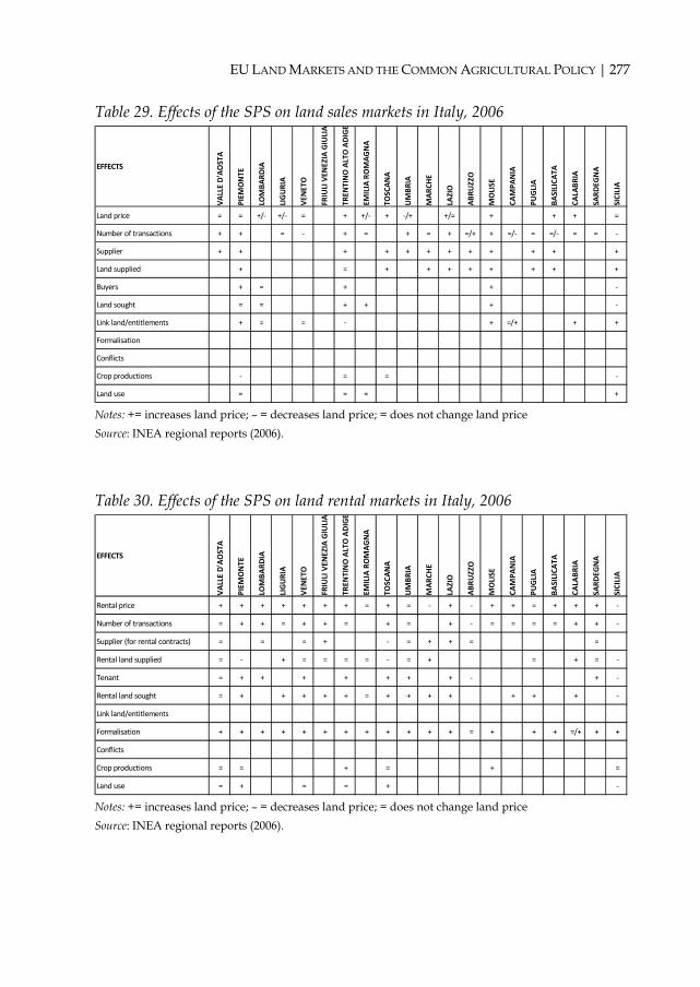
EU LAND MARKETS AND THE COMMON AGRICULTURAL POLICY | 277
Table 29. Effects of the SPS on land sales markets in Italy, 2006
EFFECTS
VALLE D'AOSTA
PIEM
ONTE
LOMBA
RDIA
LIGURIA
VEN
ETO
FRIULI VEN
EZIA GIULIA
TREN
TINO ALTO ADIGE
EMILIA ROMAGNA
TOSCANA
UMBRIA
MARC
HE
LAZIO
ABRU
ZZO
MOLISE
CAMPA
NIA
PUGLIA
BASILICA
TA
CALA
BRIA
SARDEG
NA
SICILIA
Land price = = +/‐ +/‐ = + +/‐ + ‐/+ +/= + + + =
Number of transactions + + = ‐ + = + = + =/+ + =/‐ = =/‐ = = ‐
Supplier + + + + + + + + + + + +
Land supplied + = + + + + + + + +
Buyers + = + + ‐
Land sought = = + + + ‐
Link land/entitlements + = = ‐ + =/+ + +
Formalisation
Conflicts
Crop productions ‐ = = ‐
Land use = = = + Notes: += increases land price; – = decreases land price; = does not change land price Source: INEA regional reports (2006).
Table 30. Effects of the SPS on land rental markets in Italy, 2006
EFFECTS
VALLE D'AOSTA
PIEM
ONTE
LOMBA
RDIA
LIGURIA
VEN
ETO
FRIULI VEN
EZIA GIULIA
TREN
TINO ALTO ADIGE
EMILIA ROMAGNA
TOSCANA
UMBR
IA
MARC
HE
LAZIO
ABR
UZZO
MOLISE
CAMPA
NIA
PUGLIA
BASILICA
TA
CALA
BRIA
SARD
EGNA
SICILIA
Rental price + + + + + + + = + = ‐ + ‐ + + = + + + ‐
Number of transactions = + + = + + = + = + ‐ = = = = + + ‐
Supplier (for rental contracts) = = = + ‐ = + + = =
Rental land supplied = ‐ + = = = = ‐ = + = + = ‐
Tenant = + + + + + + + ‐ + ‐
Rental land sought = + + + + + = + + + + + + + ‐
Link land/entitlements
Formalisation + + + + + + + + + + + + = + + + =/+ + +
Conflicts
Crop productions = = + = + =
Land use = + = = + ‐ Notes: += increases land price; – = decreases land price; = does not change land price Source: INEA regional reports (2006).

278 | TABLES
Table 31. Regional distribution of land prices per group of agricultural areas in the Netherlands
Region Median price index for agricultural land
1993 2000 2003 2007 Change
1993–2007 (%)
IJsselmeerpolders 1.58 2.48 4.9 4.45 182 Westelijk Holland 1.94 4.14 5 5.41 179 Zuidwestelijk Akkerbouwgebied 1.27 3.25 3.17 3.45 172 Centraal Veehouderijgebied 1.95 3.85 4.07 4.47 129 Rivierengebied 1.93 4.57 4.44 4.38 127 Veenkoloniën en Oldambt 1.01 2.54 2.3 2.25 123 Bouwhoek en Hogeland 1.25 3.37 2.26 2.72 118 Waterland en Droogmakerijen 1.24 3.05 2.1 2.61 110 Noordelijk Weidegebied 1.25 2.93 2.33 2.54 103 Zuidwest-Brabant 2.04 4.49 4 4 96 Hollands/Utrechts Weidegebied 1.81 3.75 3.36 3.5 93 Zuidelijk Veehouderijgebied 2.31 4.08 3.86 4.14 79 Zuid-Limburg 2.07 3.84 3.8 3.61 74 Oostelijk Veehouderijgebied 2.21 3.74 3.4 3.4 54
Source: Kadaster (Dutch Land Registry Office).
Table 32. Agricultural land sales prices in Sweden, 2005 and 2006 (€/ha) 2005 2006 Agricultural land (arable and grazing land) 3,350 3,706 Arable land 3,868 4,247 Grazing land 1,616 1,934
Sources: Statistics Sweden (2008) and the Swedish Board of Agriculture (2008).
Table 33. Share of rented land of the total UAA in Sweden (%) 1990 1995 1999 2003 2005
43 45 46 45 40 Sources: Statistics Sweden (2008) and the Swedish Board of Agriculture (2008).

EU LAND MARKETS AND THE COMMON AGRICULTURAL POLICY | 279
Table 34. Increase in English land values between 2004 and 2007 Type of land (%)
Prime arable 91 Average arable 97 Average livestock 104 Prime dairy 82 Poor arable 117 Poor livestock 127 All types of land 95
Source: Thomson and Renwick (2008).
Table 35. Studies on the estimated impact of subsidies on farmland values Estimated value/NPV of subsidies (market return)*
Study Dependent/ explanatory variables (country)
Land price elasticity of a 1% increase in subsidies/ returns
Estimated effect of $1/€1 of subsidy on increase in land value
r=5% r=10%
Market return Duvivier et al. (2005)
Arable land prices/market return (Belgium)
0.18-0.24 – – –
Goodwin et al. (2005)
Land prices/ market return (US)
– 6.4-7.2 0.32-0.36 0.64-0.72
Taylor and Brester (2005)
Land prices/ market return (US)
0.16-0.32 3.85-7.58 0.19-0.38 0.39-0.76
Coupled subsidies Goodwin et al. (2003)
Farmland value/LDP (US)
– 6.6 0.33 0.66
Duvivier et al. (2005)
Arable land prices/cereal compensatory payments (Belgium)
0.12-0.47 – – –
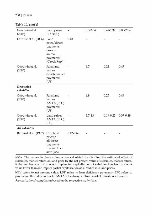
280 | TABLES
Table 35. cont’d Goodwin et al. (2005)
Land price/ LDP (US)
– 8.3-27.4 0.42-1.37 0.83-2.74
Latruffe et al. (2006) Land price/direct payments (area or animal payments) (Czech Rep.)
0.13 – – –
Goodwin et al. (2003)
Farmland value/ disaster-relief payments (US)
– 4.7 0.24 0.47
Decoupled subsidies
Goodwin et al. (2003)
Farmland value/ AMTA (PFC) payments (US)
– 4.9 0.25 0.49
Goodwin et al. (2005)
Land price/ AMTA (PFC) (US)
– 3.7-4.9 0.19-0.25 0.37-0.49
All subsidies Barnard et al. (1997) Cropland
prices/ all direct payments received per acre (US)
0.12-0.69 – – –
Notes: The values in these columns are calculated by dividing the estimated effect of subsidies/market return on land price by the net present value of subsidies/market return. If the number is equal to one it implies full capitalisation of subsidies into land prices. A value lower than one implies partial capitalisation of subsidies into land prices. NPV refers to net present value; LDP refers to loan deficiency payments; PFC refers to production flexibility contracts; AMTA refers to agricultural market transition assistance. Source: Authors’ compilation based on the respective study data.

EU LAND MARKETS AND THE COMMON AGRICULTURAL POLICY | 281
Table 36. Studies on the estimated impact of subsidies on farmland rents Study Dependent/explanatory
variables (country)
Estimated effect of $1 of subsidy on land value increase
Market return
Goodwin, Mishra and Ortalo-Magné (2005)
Land rent/market return (US)
0.35
Lence and Mishra (2003) Land rent/market return (corn revenues and soybean revenues) (US)
0.30-0.38
Coupled subsidies
Goodwin, Mishra and Ortalo-Magné (2005)
Land rent/LDP (US) 0.83
Lence and Mishra (2003) Land rent/LDP (US) -0.24
Decoupled subsidies
Goodwin, Mishra and Ortalo-Magné (2005)
Land rent/AMTA (PFC) (US)
0.29
Lence and Mishra (2003) Land rent/PFC (US) 0.71-0.86 Lence and Mishra (2003) Land rent/MLA (US) 0.84-0.90 All subsidies
Roberts, Kirwan and Hopkins (2003)
Land rents/all government payments (PFCs + conservation programmes) (US)
0.34-0.41
Kirwan (2005) Land rents/all government payments (PFCs + conservation programmes) (US)
0.20-0.40
Notes: LDP refers to loan deficiency payments; PFC refers to production flexibility contracts; MLA refers to market loss assistance; AMTA refers to agricultural market transition assistance. Source: Authors’ compilation based on the respective study data.

282 | TABLES
Table 37. SPS capitalisation into land values SPS model
Regional Historical Hybrid
Full Full,
%100=frα
Partial or full, f
rf
h αα ≤
Partial or full, f
hf
m αα ≥
Partial Partial,
fr
pr αα <
Partial, pr
ph αα <
Partial, ph
pm αα >
New entrant eligibility for entitlements
None Zero,
0=nrα
Zero,
0=nhα
Zero,
0=nmα
Notes: jiα measures capitalisation of the SPS into land values. If %100=f
rα , this implies full capitalisation of the SPS into land values. Subscripts i = r, h and m denote the implementation model: r stands for regional model, h stands for historical model and m stands for hybrid model. Superscripts j = f, p and n denote new-entrant eligibility for entitlements: f stands for full new-entrant eligibility, p stands for partial new-entrant eligibility and n stands for no new-entrant eligibility for entitlements.
Source: Model results.
Table 38. SPS capitalisation into land values and effects on restructuring with asymmetric productivity changes
SPS model
Regional Historical Hybrid
Restructuring
Full Full Partial or full
Partial or full
May be constrained with the historical and hybrid models
Partial Partial Partial Partial Constrained None Non-
tradable entitlement
Partial Partial Partial Constrained
Entrant eligibility for entitlements
None Tradable entitlement
Zero Zero Zero Not constrained
Source: Model results.

| 283
APPENDIX 1. LITERATURE REVIEW
Introduction Various studies have the analysed agricultural policy measures that have been implemented to support farmer income in developed countries, such as market price support, production subsidies, factor subsidies, coupled and decoupled payments (see e.g. Hertel, 1989; Salhofer, 1996; Dewbre et al., 2001; Alston and James, 2002; Guyomard et al., 2004; Ciaian and Swinnen, 2006 and 2007).
The common conclusion of these studies is that the agricultural policies implemented affect (increase) farmer income, although to a varying degree depending on the policy. In addition to this direct first-order effect, most of the agricultural policies also induce further, second-order adjustments. For example, farm subsidies influence not only the employed factor reward but also, through altered farmer incentives, factor demand, inter-sectoral factor allocation and factor ownership. While the number of studies looking at these issues has grown in the last decade, the impact of the second-order effects has been investigated insufficiently in the empirical literature (Bullock and Salhofer, 2003; OECD, 2007; Alston, 2007).
One strand of the literature assessing second-order impacts considers the consequences of policy for land prices and land rents. These insights are crucial as they may help answer some politically important questions concerning subsidies: Who benefits from the subsidies and how much – landowners or farmers renting the land? How is agricultural productivity affected? How do the subsidies and their consequences affect future policy design?
If agricultural subsidies benefit landowners instead of farmers, negative side effects may arise. For example, policy-induced growth in land values might reduce efficiency in the agriculture sector. Given that farmers must finance a higher initial investment (entry cost) and face the risk that policy changes may affect the return on that investment, the entry barrier for potential new farmers increases. The expansion costs for existing farmers also rise. Consequently, the transfer among different owners is reduced, pushing up the average costs of production in the agricultural sector.
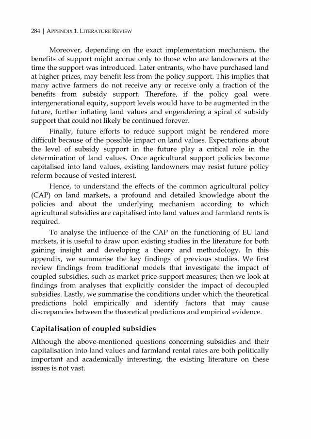
284 | APPENDIX 1. LITERATURE REVIEW
Moreover, depending on the exact implementation mechanism, the benefits of support might accrue only to those who are landowners at the time the support was introduced. Later entrants, who have purchased land at higher prices, may benefit less from the policy support. This implies that many active farmers do not receive any or receive only a fraction of the benefits from subsidy support. Therefore, if the policy goal were intergenerational equity, support levels would have to be augmented in the future, further inflating land values and engendering a spiral of subsidy support that could not likely be continued forever.
Finally, future efforts to reduce support might be rendered more difficult because of the possible impact on land values. Expectations about the level of subsidy support in the future play a critical role in the determination of land values. Once agricultural support policies become capitalised into land values, existing landowners may resist future policy reform because of vested interest.
Hence, to understand the effects of the common agricultural policy (CAP) on land markets, a profound and detailed knowledge about the policies and about the underlying mechanism according to which agricultural subsidies are capitalised into land values and farmland rents is required.
To analyse the influence of the CAP on the functioning of EU land markets, it is useful to draw upon existing studies in the literature for both gaining insight and developing a theory and methodology. In this appendix, we summarise the key findings of previous studies. We first review findings from traditional models that investigate the impact of coupled subsidies, such as market price-support measures; then we look at findings from analyses that explicitly consider the impact of decoupled subsidies. Lastly, we summarise the conditions under which the theoretical predictions hold empirically and identify factors that may cause discrepancies between the theoretical predictions and empirical evidence.
Capitalisation of coupled subsidies Although the above-mentioned questions concerning subsidies and their capitalisation into land values and farmland rental rates are both politically important and academically interesting, the existing literature on these issues is not vast.

EU LAND MARKETS AND THE COMMON AGRICULTURAL POLICY | 285
The classical model for analysing income distributional consequences of agricultural support policies is Floyd (1956). Floyd proposed a model with two factors used to produce one agricultural output. He assumed one land and one non-land (labour and capital) input, which are combined in a constant returns-to-scale production function. In his model, output market clearing and input market clearing determined the output and input prices. The elasticities of factor supply and the elasticity of demand were assumed constant.
According to Floyd’s canonical model of two inputs and a single output, price support increases the price of a factor if its supply is not perfectly elastic. A given percentage increase in product price will result in the same percentage rise in all factor prices if inputs are perfect substitutes in production or if the supply elasticities of the two factors are the same. If the factor supply elasticities are not equal, the price of the input with the least elastic supply will rise most.
In Floyd’s model, the income distribution of agricultural support policies depends largely on the input supply and input substitution elasticities. For policy purposes, we can distinguish between two situations: i) factor supply is either perfectly elastic or perfectly inelastic and there is zero elasticity of substitution between factors (the corner solution of the model); and ii) factor supply is partially elastic and there is positive elasticity of substitution between factors (the interior solution of the model).
First, consider the corner solution when factor supply is entirely inelastic and the elasticity of substitution between factors is zero. According to the corner solution of Floyd’s (1956) model, output price support simply inflates input costs, and the value of output support becomes captured in the value of the factor with inelastic supply. If the inelastic factor is land, then the value of subsidies is fully captured into land rental rates, and therefore capitalised into land prices. If the factor owner is a farmer, then the agricultural support policy increases the farmer’s income. Otherwise, the benefit of the agricultural support policy leaves the agricultural sector and it is captured by the non-farming landowner.
Moreover, on an intergenerational basis, by increasing the cost structure of production, the agricultural support policy increases the set-up cost for future farmers as they have to ‘buy’ the value of the policy support

286 | APPENDIX 1. LITERATURE REVIEW
as a condition for entry into the sector.94 This in turn implies that to the extent to which price support is capitalised, it will benefit active farmers at the time the policy support is introduced more than ex-post start-ups.
Second, consider the interior solution when factor supply is inelastic but the elasticity of substitution between factors is positive. According the interior solution of Floyd’s (1956) model, the effects of output price support on output and factor markets depend on the factor supply elasticity. In other words, the more inelastic is the factor supply, i) the more the output price increase is translated into a higher price of that factor, ii) the more the price support indirectly increases the production cost of the output and iii) the smaller is the induced increase in the farmer’s profit, as the value of support provided through the output price is transferred to the owner of the factor.
The main findings of the theoretical literature on coupled policy impacts can be summarised as follows (with area payments being coupled payments as they were in the EU before the introduction of the single payment scheme (SPS)): • If land supply is fixed, then area payments are fully capitalised into
land value. • Coupled production subsidies are fully capitalised into land values if
in addition to a land supply elasticity of zero either the supply elasticity of non-land inputs is perfectly elastic or the factor proportions are fixed.
• In other situations, the benefits from coupled subsidies are shared between land and other production factors, and if demand elasticity is not perfectly elastic, the consumers as well.
• The impact of agricultural policy on land values may be very large (e.g. fully capturing the subsidies).
94 In a legal business environment – where farms are more or less inherited free of taxes, charges and compensatory payments by family members not staying in the farm business – the intergenerational equality argument applies only to those farms that want to expand in acreage or newly enter the system.

EU LAND MARKETS AND THE COMMON AGRICULTURAL POLICY | 287
Capitalisation of decoupled subsidies More recently, a new generation of partial and general equilibrium models has been developed to analyse explicitly the impact of decoupled subsidies. Most of this literature, which is still at an early stage of development, is based on behavioural models of profit maximisation. The two most prominent representatives of this class of models are Guyomard et al. (2004) and Ciaian and Swinnen (2006 and 2007).
By their definition, fully decoupled policies should not affect agricultural markets generally or land markets specifically (Cahill, 1997; OECD, 2001). Ciaian and Swinnen (2006) proposed a partial equilibrium model for analysing the income distributional effects of area payments and the SPS. In this model, they assume two heterogeneous farms competing for land. Each of the two heterogeneous farms maximises profits. Ciaian and Swinnen assume one input (land) and one output, and that the total land supply is fixed.
Ciaian and Swinnen find that a decoupled subsidy that is not linked to the output market or input market does not affect marginal output or marginal input profitability. Thus, a fully decoupled payment does not influence farmers’ behaviour and has no income distributional effects. Furthermore, a truly decoupled policy does not shape long-term adjustments in the agricultural sector. Ciaian and Swinnen also show that the SPS does not affect land values. These results hold even if the SPS is not fully decoupled because, for example, farmers need to have eligible land to activate SPS entitlements.
The main findings of the theoretical literature on decoupled policy impacts can be summarised as follows: • Fully decoupled farm policies have no impact on land values if
markets are perfect. • Decoupled policies may affect land values only in the presence of
(some) market imperfections (such as land-market transaction costs or credit constraints).
• The exact impact depends on many factors, such as policy type, supply and demand elasticities, accompanying policy measures, market imperfections, land-use opportunity costs, institutions and expectations.

288 | APPENDIX 1. LITERATURE REVIEW
Determinants of subsidy capitalisation The exact outcome of the policies implemented in terms of income distribution, inter-sectoral factor allocation and factor productivity is affected by many things. As noted above, the determinants related to policy are the policy type, implementation details and associated measures. The principal determinants related to exogenous comparative advantage (endowment and technology) are factor supply and substitution elasticities, and possibilities for inter-sectoral production substitution (land-use alternatives). The determinants connected with the land market include market imperfections, land market institutions and regulations, and transaction costs. Finally, the outcomes of farm support policies depend on the timescales policy-makers are looking at and on the responsiveness dynamics of those policies.
In this section, we review the most important of these factors, which in mutual interaction, determine the direction and extent of effects induced by coupled and decoupled agricultural policies with respect to factor income in general, and land rents and prices in particular.
Policy type For the most part, various policies can be implemented to address the policy objective of supporting farmer income, such as subsidies for inputs, outputs and exports; decoupled payments; and quotas on inputs and outputs. A conclusion from the theoretical literature is that one of the key factors that determine the extent to which subsidies are captured in land values is the type of policy implemented. This result holds for not only decoupled versus coupled policies, but also for the significant differences among the diverse coupled policies.
For example, consider the impacts of an output subsidy and an area payment. An area payment is targeted directly at land while an output subsidy is linked to agricultural output. Because an area subsidy is directly linked to the land market, it is expected to have a stronger impact on land values than an output subsidy. It decreases farms’ land costs, which in turn increases the demand for land. A land subsidy solely decreases land costs, leaving the rest of the input costs unaffected. Higher land demand in turn exerts upward pressure on land prices. In contrast, an output subsidy affects land prices indirectly through a higher profitability of agricultural production. It has a direct influence on the output market and consequently the welfare of consumers. Indirectly, an output subsidy stimulates demand

EU LAND MARKETS AND THE COMMON AGRICULTURAL POLICY | 289
not only for land but also for all farm inputs. Therefore, it affects the marginal profitability of all farm inputs equally. As a result, the effect of the subsidy is shared equally among all the inputs (OECD, 2007).
Policy implementation details The capitalisation rate of subsidies is also contingent upon policy implementation details. For example, depending on whether the subsidies are available for a certain period or are ‘open-ended’, their capitalisation into land values may be different. Benefits may flow to landowners but may not be capitalised into land values if they are not expected to continue into the future. On the other hand, benefits may be capitalised effectively into land values even if the benefits themselves do not flow to land per se.
From the SPS perspective, a critical aspect is the mechanism used for the allocation of entitlements. If the right to a stream of income is freely transferable separately from land or other assets, then the value of that stream will be capitalised into the entitlement (Alston, 2007). But if entitlements are attached to land and cannot be used or transferred separately from that land, then the subsidy is likely to be capitalised effectively into the value of the land or the farm as a whole. Alternatively, if a right to entitlements is assigned to an individual, separately from land or any other assets and not in any way transferable, it will not be capitalised into any physical assets.
The degree to which the SPS entitlements are capitalised into land values additionally depends on the SPS model chosen (historical, regional or hybrid) and the ratio of entitlements to land (Kilian and Salhofer, 2008).
If the number of hectares exceeds the number of entitlements, the single payments are not capitalised into land prices. This is true for all three SPS models. Ultimately, it is the number of suppliers and demanders on the entitlement market that will determine the outcome. If there is a surplus of demand, entitlements will have their own value decoupled from land.
If the number of entitlements exceeds the number of hectares, the outcome is different for all three models. In the case of the historical model, a portion of the single payments is capitalised into land values. The degree of capitalisation depends on the proportion of single payment entitlements to land and the variability of single payments. In the extreme case of identical single payments for each hectare, the result is the same as in the regional model with all rents from entitlements capitalised into land values.

290 | APPENDIX 1. LITERATURE REVIEW
In the case of the hybrid model, the level of capitalisation lies somewhere between the other two models (given the same overall single payments).
Thus, based on the policy implementation details, decoupled subsidies may be fully capitalised into land or not capitalised into land at all. Depending on the rules determining eligibility to receive the future stream of policy transfers, they may also be only partially capitalised into the land values (Sumner and Wolf, 1996; Ciaian and Swinnen, 2006; Ciaian et al., 2008; Kilian and Salhofer, 2008).
Accompanying policy measures In the real world, agricultural support policies are combined in policy programmes involving multiple instruments working at the same time, none of which can be considered isolated from the others. Hence, even when farm payments are fully decoupled (as in the case of the SPS), whether the payments are fully reflected in land rents or capitalised into land values may be dependent upon other policy instruments.
Given that the vast majority of decoupled policies are combined with coupled policy instruments in one way or another, they are not fully decoupled. As such, their ultimate effects will also be conditioned by the extent to which the effects shift through changes in input use and output, which in turn depends on the details of the policies and parameters of supply and demand and so on.95 For example, decoupled payments and area payments may be subject to cross-compliance, set-aside or other requirements. If area payments are subject to cross-compliance, then their
95 According to Alston (2007), in the presence of other policies, the results of econometric studies might be affected by the mechanism of how policies are represented in the models. Econometric studies often require some aggregation across different types of subsidies in ways that may cause problems if the nature of the subsidies varies across the observations (for example, the mixture of forms of subsidies varies in a cross-section or the details of the instruments change over time).

EU LAND MARKETS AND THE COMMON AGRICULTURAL POLICY | 291
effect on land values is mitigated because the eligibility for subsidies requires farmers to incur certain costs.96
Factor supply elasticity As outlined above, the exact influence of subsidies on land values is linked to the factor supply elasticity.97 In an extreme case, the factor supply elasticity may even reverse the original effect of subsidies on land values.
In the case of small substitution elasticities, any subsidy will have a substantial impact on land values. With the introduction of subsidies, most of the adjustments take place through price changes while adjustments in quantity are small. In the case of area payments, a large proportion of subsidies will be capitalised into the land price. In an extreme scenario, when the supply elasticity of land is zero, then area payments are fully capitalised into land values.
When land supply elasticity is positive, area payments will likewise affect the prices of other inputs as well as prices of agricultural commodities. Concerning supply-elastic inputs, markets respond to policies by a sharp adjustment in quantity and a small adjustment in price. Output subsidies lead to a higher increase in the price of supply-inelastic inputs than the price of supply-elastic inputs. Output subsidies are fully capitalised into land values only when the supply elasticity of land is zero and when the supply elasticity of non-land inputs is perfectly elastic (Floyd, 1965; Gardner, 1983; Alston and James, 2002).
In empirical studies, the land supply elasticity is usually found to be rather low, mostly owing to natural constraints. For example, based on an extensive literature review, Salhofer (2001) concludes that a plausible range
96 Ciaian and Swinnen (2006) show in the case of the SPS that when an entitlement providing a right to an area subsidy is owned by a farm and is allocated to a fixed quantity of land, then the subsidy is not capitalised into the land value. Instead, the subsidy benefits the farmer. In this situation, the subsidy does not affect the marginal return of the rented land. This is contrary to the effect of an area subsidy granted per hectare, which becomes capitalised into the land value. 97 The supply elasticity measures how factor supply responds to price changes. If an input is supply-inelastic, then policies will have a large impact on the price and a small impact on the quantity of that input.

292 | APPENDIX 1. LITERATURE REVIEW
of land supply elasticity for the EU is between 0.1 and 0.4. Similarly, Abler (2001) finds a plausible range between 0.2 and 0.6 for the US, Canada and Mexico.
Land-use alternatives Usually, land can be used not only by agriculture but also by other sectors of the economy. If there is such an opportunity, land values will reflect this potential, alternative land use. In a competitive market, land values reflect returns from the most profitable use of land. If the most profitable use of land is non-agricultural (e.g. urban housing), then land values will be determined by the profitability of urban housing. But if the non-agricultural use of land is expected to be profitable in the future, then the current land price will reflect the sum of the discounted stream of rents from agriculture up to the time of conversion plus the discounted stream of expected rents from non-agricultural use from that time onward (Plantinga et al., 2002).
Factor substitution elasticity Substitution elasticity is a further crucial factor determining the distributional consequences of policies.98 With area payments, farms have an incentive to substitute land for other inputs, which expands land demand and leads to significant capitalisation of subsidies into land values. Subsidies that are not targeted at land have the opposite effect.
Where there is a high elasticity of substitution between land and other inputs, the impact of the area subsidy on land values that is induced will be large, as a high elasticity of substitution allows easy substitution between land and other farm inputs in the production process. In general, a high elasticity of substitution between land and other farm inputs reduces the impact on land values in the case of subsidies not tied to land (Floyd, 1965; Gardner, 1983; Alston and James, 2002).
Based on 32 studies, Salhofer (2001) reports average elasticities of substitution between land and labour of 0.5, between land and capital of 0.2, and between land and variable inputs of 1.4 for Europe. Similar values are reported in Abler (2001) for the US and Canada.
98 Substitution elasticity measures how easy it is to substitute one input for another in the farm production function.

EU LAND MARKETS AND THE COMMON AGRICULTURAL POLICY | 293
Market imperfections and transaction costs In the presence of market imperfections, the policy impact realised might vary from that predicted by models with perfect competition. Indeed, several studies show that decoupled payments affect farm behaviour differently in the presence of market imperfections from a situation with perfect competition (e.g. Chau and de Gorter, 2005; Hennessy, 1998).
Generally, land transaction costs related to land withdrawal from corporate farms in transition countries do not affect the overall result that area payments increase land rents and benefit landowners instead of farmers (Ciaian and Swinnen, 2006). Yet, transaction costs depress land prices both with and without area payments. Transaction costs and area payments have the opposite effect on land rents. Transaction costs reduce land rents, while area payments are capitalised into land rents. If the effects are equal then they cancel each other out.
Also, credit market imperfections have important implications for the distribution of area payments (Ciaian and Swinnen, 2007). In a model with land as a fixed factor and credit market imperfections, area payments increase land rents more than subsidies do. On aggregate, farms may actually lose rather than benefit from the subsidy – only the most credit-constrained farms may gain from the subsidy.
Land market institutions and regulations The effect of subsidies on land values in competitive markets can be influenced by land market regulations. The most obvious one that will affect the land market is the regulation of land prices (e.g. fixed) by the government (Latruffe and Le Mouël, 2006).
Various formal and informal institutions in land markets will similarly affect the subsidy–land value relationship. For example, if a rental agreement is for a purely ‘cash’ rental arrangement, then the farm programme payments must go entirely to the farm operator; the landowner is not eligible to receive any payments. Otherwise, under a share rental arrangement, the same subsidy payments may have to be divided between the landowner and the tenant. With crop-sharing contracts, the issue is more complicated in that production flexibility contracts (PFCs) are

294 | APPENDIX 1. LITERATURE REVIEW
supposed to be shared in proportion to crop shares.99 If the terms of such leases are not adjusted, the landowner will not reap the full benefits. Thus, if subsidy payments increase unexpectedly in the presence of pre-existing leases, tenants holding a cash rental arrangement will capture all of the benefits (and their landowners will receive none), whereas tenants holding a share rental arrangement will divide these same benefits with their landowners.
Obviously, these regulations govern only the initial distribution of subsidy payments between landowners and tenants, which is almost certainly different from the outcome after markets have adjusted to the new equilibrium with subsidies. Other things being equal, one would expect that the rates of cash rentals would adjust to equivalence with the corresponding share rental rates, reflecting the subsidies and other determinants of income.
Social capital Farmers are working and living not only in an economic but also in a social and cultural context. Therefore, the actual decisions of a farmer in a given market are influenced by the intensity and kinds of social relationships of the parties involved in a transaction and by the societal norms and cultural context (Robinson and Flora, 2003). Studies for the US show that social capital is a pivotal factor for the land market, influencing the type of transaction (e.g. Rainey et al., 2005), the price of the land (Robison et al., 2002) and the parties involved in the transaction (Siles et al., 2000). Thus, the extent to which subsidies are incorporated in farmland values and therefore transferred from the farmer to the landowner also depends on the local cultural and social setting.
Land transactions occur mainly between relatives or friendly neighbours (Siles et al., 2000). These groups receive a rebate on the land price ranging from 10% (Robison et al., 2002) to 43% (Tsoodle et al., 2006) compared with total strangers. According to Tsoodle et al. (2006), the influence of social capital has grown over the last few years. With respect to rental contracts, social capital influences the type of the contract while the
99 Barnard et al. (2001) report the testimony of a panel of farm managers that with cash rentals, the terms of leases are negotiated with “lease rates being bid up until the landowner had captured most of the tenant’s share of the PFC”.

EU LAND MARKETS AND THE COMMON AGRICULTURAL POLICY | 295
rental price is inversely correlated to the duration of the relationship between the landowner and tenant (Rainey et al., 2005).
Time scale and dynamics The impact of both coupled and decoupled policies varies over time. For example, formal and informal land rental contracts imply that the transmission of changes in policy into rental prices and asset prices for land is not instantaneous. The sluggish adjustment of rental rates suggests that the short- and intermediate-term results of policies will be different from the long-term outcome with complete adjustment. Moreover, even without contracting, land markets involve lags and dynamics, uncertainty and expectations. For example, rental arrangements are typically multiyear in their nature and often reflect long-term personal relationships or family members. Competitive pressures might not take full and immediate effect in such a setting (Gardner, 2002).
Furthermore, data on land rents and land values are often based on expert assessments rather than direct evidence from market transactions. These assessments are likely to understate the true movements in rental prices associated with yearly variations in income stemming from the market or from transfers. Because contracts are established well in advance of market realisations, they do not precisely correspond to the observed realisation. For instance, land rents are set ex ante whereas subsidy payments can only be observed ex post.
All of these factors imply that short-term movements in rental prices will be different (lower) than the long-term impact of permanent changes in subsidies.
Simulation studies The theoretical models discussed in the previous section have been applied in two kinds of empirical studies: i) ex ante simulations of policy impacts and ii) econometric estimations, in terms of providing the functional relationship and hypothesis. In this section, we summarise the findings of key simulation studies. More precisely, we review the three most influential studies on land markets in the EU, which among other

296 | APPENDIX 1. LITERATURE REVIEW
important questions investigate the impact of agricultural subsidies on land values and farmland rental rates: SCENAR 2020, GENEDEC and IDEMA.100
The SCENAR 2020 study simulates the major trends that will form the framework for the European agricultural and rural economy by 2020. Among the main driving forces, SCENAR 2020 identifies rural demographic patterns, agricultural technology, agricultural markets and the natural and social constraints on land use that are likely to exist in 2020.
By comparing the reference scenario with two alternative scenarios (‘liberalisation’ and ‘regionalisation’), the SCENAR 2020 project investigates and compares the effects of three different policies. In the baseline (reference) scenario, all current policies are considered to continue into the future, with modifications over time that are reasonably certain to happen according to the present political situation. In the regionalisation scenario, there is a sustained policy preference to promote regional economic strength and social welfare; to some extent, this is also an emphasis on the maximum degree of support for agricultural supply that is possible under the current, and likely, WTO framework. In the third (liberalisation) scenario, policy intervention in the economy and in social welfare, including environmental protection, is reduced to a socially acceptable minimum.
The simulation results of SCENAR 2020 suggest that factor markets have general trends that are rather independent of policy, except for agricultural land prices, which decrease significantly because of market liberalisation. The simulated development of factor prices shows that especially land prices are very dependent on the policy instruments implemented. The direct payments and profitability of agriculture accrue partly in the price of the fixed factor of land. In the regionalisation scenario, direct payments remain highest and agriculture is more profitable relative to other scenarios, and land prices are the highest. In the liberalisation scenario, land prices decline considerably, because all direct payments are abolished and profitability in agriculture falls. Declining prices of agricultural land imply lower asset values for the landowners. This might affect the viability of landowners who are heavily indebted. Depending on
100 The GENEDEC and IDEMA studies were financed by the 6th EU Framework Programme for Research and Technological Development. SCENAR 2020 was financed by the European Commission, DG AGRI.

EU LAND MARKETS AND THE COMMON AGRICULTURAL POLICY | 297
whether landowners are farmers and whether they live in urban areas, this could lead to adjustment costs in rural areas, which could in turn justify adjustment policies.
GENEDEC performs socio-economic and environmental assessments of decoupling measures, by using a set of simulation models for various regional levels. More precisely, it provides insights into the workability, the efficiency and the impacts of various scenarios of decoupling; it undertakes quantitative assessments of the impact of a decoupled support scheme on production, land use and land prices. Thanks to a complete set of databases (including the FADN farm-level data), GENEDEC covers the entire EU.
The GENEDEC project adopts a simplified approach to assessing the effects of subsidy decoupling on land values (dual values of land equations) for i) single farm groups and ii) land trade constraints for all farms within regions. GENEDEC compares the total shadow price with the rental land value, taking note of the fact that here labour is not accounted for (the difference between the shadow price and the rent could be considered a proxy of the average marginal value of the labour time spent on one hectare).
GENEDEC relates different compounds of the land shadow prices to the prices and to the constraints existing in the model for which the total utilised agricultural area (UAA) is explicitly used. GENEDEC relates the ‘land’ compound to the availability of the land fixed factor (‘UAA’), and the shadow price implicitly takes account of all payments connected with agricultural activities.
In a case study for Italy, GENEDEC simulates the percentage changes in factor prices. They find that only the price of land varies regionally. In the total decoupling scenario, the simulated regional land price increases are as follows: 16.28% nationally, 20.39% in the north, 12.30% in the centre and 14.86% in the south. These simulation results suggest that higher land prices, especially in the north of Italy, are expected to curb transactions of land properties, but may activate the rental market for land.
The IDEMA study provides a comprehensive socio-economic assessment of the impact of decoupling on the EU farming sector. The project assesses the consequences of decoupling for market demand and supply, trade, localisation of production, land use, the environment, land markets, structural change, farm income and farmers’ entry/exit behaviour. The IDEMA project is organised around three complementary, empirical approaches: a survey-based analysis of farmers’ strategic

298 | APPENDIX 1. LITERATURE REVIEW
decisions, dynamic, farm-based regional modelling and sector-level and general equilibrium modelling.
By performing numerical simulations, IDEMA analyses the socio-economic impacts of decoupling EU agricultural support in three distinct decoupling scenarios: i) actual implementation of the 2003 CAP reform (as implemented in each member state); ii) full decoupling with fully decoupled direct payments and top-ups; and iii) a bond scheme, whereby the SPS is linked to the farmer and not to land.
IDEMA’s results reveal that the impacts of the 2003 CAP reform are moderate, compared with a continuation of Agenda 2000. According to the IDEMA’s simulation results, there is no significant evidence that farmers would drastically change their strategic decision to exit agriculture. In fact, IDEMA’s results indicate that structural change slows down when direct payments are decoupled. One reason for this effect is that grassland management becomes an additional income source for farmers. Another key finding of IDEMA is that the decoupled payments may reduce farmers’ off-farm labour supply. In the new member states, the impact of accession dominates the effects of decoupling. IDEMA’s simulation results show that the introduction of CAP payments results in a greater willingness to stay in farming and more competition for land. Increased payments are capitalised into higher land (rental) prices.
IDEMA’s simulation results suggest that the bond-type decoupled payment would lead to a sharp increase in average farm size compared with the 2003 CAP reform. Many farmers would leave the sector if off-farm jobs were available, as the decoupled payment is granted to a farmer independent of land or any farming activity (it is only based on historical production). But in most cases, profits per hectare do not change or even increase under the bond scheme, owing to significantly lower land (rental) prices and structural change.
Findings from the EU simulation studies suggest that agricultural policies do affect land prices and land rental rates. In line with the theoretical literature on subsidy capitalisation, the scenario analyses performed suggest that subsidy capitalisation into land values and land prices depends on both policy and non-policy assumptions, which were compared across scenarios.

EU LAND MARKETS AND THE COMMON AGRICULTURAL POLICY | 299
Empirical studies on land (sales) prices The empirical attempts to estimate the impact of agricultural support policies on land rents and land prices can be grouped into two broad categories: land value/price studies and land rent studies. Whereas the former examine the effects of policies on farmland prices, the latter investigate the policy impacts on farmland rental rates. The main reason authors use one approach over another is usually data: the availability of either land value (typically from regional datasets) or rental data (typically from farm-level surveys) commonly determines the choice of model.
It is important to point out that virtually all of the existing studies are on North America (the US and Canada). To our knowledge, only three cover EU countries (Traill, 1980; Goodwin and Ortalo-Magné, 1992; Duvivier et al., 2005). Moreover, none of these measures the impact of the SPS (Table 35).101
Goodwin and Ortalo-Magné (1992) estimate an empirical model relating land values to the expected level of producer support, expected yield and expected producer prices net of subsidy support in six wheat producing regions in France, the US and Canada between 1979 and 1989.102 The subsidy support is proxied by the producer subsidy equivalent.
Goodwin and Ortalo-Magné estimate that a 50% reduction in producer support for wheat growers would lead to a $60–120 land price decrease in France and a $50–60 decrease in the US and Canada. This means that, on average, a 1% increase in the producer subsidy equivalent would increase the land value by 0.38%. Goodwin and Ortalo-Magné also find that land prices are more responsive to government-based returns than to market-based returns.
101 The large majority of empirical studies performed to date have estimated the present value of land as a function of government payments and other explanatory variables. The main reason for the relative dominance of land price studies is given by the data availability – usually regional data are more broadly available (typically used in land price studies) than farm-level data (typically used in land rent studies). 102 These were Kansas and North Dakota in the US, Manitoba and Saskatchewan in Canada and the Centre and Picardie regions in France.

300 | APPENDIX 1. LITERATURE REVIEW
Barnard et al. (1997) undertake a separate approach using pooled cross-sections in order to assess the degree of capitalisation. For investigating the consequences of public support on farmland prices, they adopt an alternative framework to the present value models. Relying on a hedonic price model, Barnard et al. regress the cropland values against government subsidies.103 They measure government payments by the county-level averages of the annual amount of direct payments received per acre for 20 US regions. To account for possible land conversion, they include proxies for alternative uses of land in their regression. The other explanatory variables they include are agricultural productivity, non-agricultural influence and state-specific institutional environments and others.
Barnard et al. find that, depending on the region, the elasticity of cropland values to the government subsidies ranges from 0 to 0.69. Based on these results they conclude that the sensitivity of farmland values to government support is spatially variable. Two elements can explain this spatial variability: i) whether the dominant crops in a given region are eligible for the support and ii) the level of agronomic flexibility of a given region, which determines the ability to adjust output in response to changing government policy. Yet, Barnard et al. fail to account for omitted variables that might determine both subsidies and land values, thereby likely failing to identify a causal relationship.
In a follow-up study, Barnard et al. (2001) analyse county-level farmland value data from the 2000 Agricultural Resource Management Study (ARMS). As in the 1997 study, Barnard et al. ran hedonic land price regressions to estimate the effect of the commodity programme payments on farmland value, while controlling for soil quality, urban influence, availability of irrigation and other factors.104 Thus, their regressions include
103 This approach relies on the idea that the land price is determined by the meeting of sellers’ and buyers’ bids, based on their respective maximised profit. Yet, in the hedonic price framework, determinants of land price are often chosen in an ad hoc way. 104 They explain the value of farmland per acre at the county level, as reported by farm operators in the 2000 ARMS conducted by US Department of Agriculture.

EU LAND MARKETS AND THE COMMON AGRICULTURAL POLICY | 301
land value per acre as a function of the commodity programme payments received, soil quality, the availability of irrigation, urban influence and other factors.
The results of the hedonic pricing model in Barnard et al. (2001) suggest substantial effects of government payments on land values. They estimate that $61.6 billion of the $312.3 billion value of land harvested for eight programme crops (wheat, corn, soybeans, sorghum, cotton, rice, barley and oats) was attributable to programme payments. Since payments received in 2000 for these programmes amounted to about $21 billion, it appears that each $1.00 of payments generates about $3.00 of land value. Their results suggest that payments have the highest proportional effect in the heartland region, accounting for 24% of farmland value. The effect is similar in the Prairie Gateway region (23%) and the Northern Great Plains region (22%).
Barnard et al. note that the very high land-value counties are urbanised areas where their prices are unlikely to be caused by commodity programmes. To account for the effects of urbanisation, they estimate separate regressions for different regions of the country and include additional right-hand side variables. Barnard et al. also realise that the current level of payments is not the source of all programme effects on land values. For example, Barnard et al. note that in 2000, a larger payment proportion than usual was made up of loan deficiency payments (LDPs), and these would be expected to have a smaller effect on land values than production flexibility contracts (PFCs) because LDPs have the additional effect of reducing commodity prices. More broadly, land values are expected to reflect not only the current year’s level of payments, but also all discounted, expected future benefits. The observational basis for farmers’ expectations about these benefits is current payments as well as recent past payments and the commodity market conditions underlying the forecasts of future payments.
Gardner (2002) uses pooled cross-sections to estimate farm subsidy impacts. Gardner finds that an additional $1.00 per acre in programme payments would have increased the average growth rate in US land values from 1950 to 1992 by 0.017%. Given that the mean value of 1992 payments per acre in the counties studied was $15.00, the elimination of the programmes would have caused the rate of increase of farmland values to

302 | APPENDIX 1. LITERATURE REVIEW
decline by 0.26%; in other words, instead of growing by 1.76% annually during 1950–92, without the programmes the rate of growth would have been 1.5%.
Overall, Gardner finds the evidence from county data that farm programmes have increased farmland values to be weak and inconclusive. Gardner also admits that the coefficient of government payments is not robust to alternative specifications that include other right-hand side variables.
Goodwin et al. (2003) use farm-level data for 1998–2001 drawn primarily from ARMS to estimate the determinants of farmland values. They estimate the capitalisation rate of government payments (PFC payments and disaster-relief payments, which include market loss assistance (MLA) payments) into farmland values. They rely on the fact that the formation of land values is based upon expectations about the long-term stream of returns attached to land. To represent the expected payment, Goodwin et al. use a four-year average value of the realised payments at the county level. In addition, they augment the canonical framework of net present value to account for possible land conversion.
Goodwin et al. first consider the aggregation of all support programmes into a single category. They show that using the actual realised payment of each farm as a proxy of the expected rent gives a coefficient of 5.40. With the county average, they obtain a coefficient of 6.09.
In addition, Goodwin et al. estimate programme-specific marginal impacts of per acre subsidies on land values that range from $2.59 to $7.78, depending on the source of the programme payment. Assuming a discount rate of 5% (10%), their results suggest that landowners capture between $0.13 and $0.39 ($0.26 and $0.78) of the marginal subsidy dollar in the form of higher land rents, and that this incidence varies by programme, i.e. they show that the rate of capitalisation of $1.00 of payment is programme-specific.
Breaking down the overall measure of government payments into their individual components, they quantify the capitalisation rate for each type of support programme.
Goodwin et al. find that the impact of an additional $1.00 of PFC payments is $4.90 per acre, which is statistically significant. They also find that disaster-relief payments have a statistically significant effect on farmland values, with the impact of an additional $1.00 of payments being about $4.70 per acre. These results suggest that both PFC and disaster-relief

EU LAND MARKETS AND THE COMMON AGRICULTURAL POLICY | 303
payments are captured at least partially by landowners, and that landowners were anticipating a continuation of payments beyond the life of the 1996 Federal Agricultural Improvement and Reform (FAIR) Act.105
Similar to Barnard et al. (1997), Goodwin et al. find that the extent to which support policies affect land values is spatially variable. They also point out that the implied effect of a support instrument on land values differs from year to year. As the authors note, one caveat to their results is that annual fluctuations in government payments may not capture the changes in long-term expectations of cash flows that drive land values. When the authors modified their model to allow the influence of government payments on land values to differ from one year to another, they found substantial differences in the effects of payments across years.106
Duvivier et al. (2005) estimate the impact of the 1992 and subsequent CAP reforms on arable farmland prices in Belgium. Using a panel of 42 Belgian districts from 1980 to 2001, they observe that the sales prices of arable farmland are affected by the compensatory payments.
The estimation results of Duvivier et al. indicate that, besides the time dummies and other control variables, the expected land rents from market sales exert a pronounced effect on arable farmland prices. Depending on the year and region considered, the elasticity of arable farmland prices to compensatory payments ranges from 0.12 to 0.47. These results suggest that, by creating a rent that capitalises into land values, the new CAP instruments also benefit landowners. Because around two-thirds of Belgian agricultural land is rented by farmers, non-operators capture an important 105 Goodwin et al. (2003) also included LDPs in their model. The impact of an additional $1.00 of LDP payments on land values is about $6.60 (2003) per acre. The effects of LDPs are somewhat larger than those estimated for PFC or MLA payments, but the authors do not indicate whether these differences are statistically significant. 106 Goodwin et al. (2003) realise several econometric issues are associated with their estimations. An assumption that the realisation of a particular source of return correctly reflects the long-term expectations could lead to an error-in-variable problem. Error-in-variable problems result in inconsistent estimators. They also note that the use of the farm-observed payments may result in an attenuation bias that forces the implied capitalisation rates towards zero. Because of the four-year county average, payments are more representative of the long-term benefits, and hence a larger coefficient is obtained.

304 | APPENDIX 1. LITERATURE REVIEW
share of agricultural subsidies. The results of Duvivier et al. also indicate that a temporal variability exists in the elasticity of arable farmland values to compensatory payments. They show that the sensitivity of arable farmland values to compensatory payments increased during the 1993–2001 period.
The main results of the principal studies on the impact of subsidies on farmland values are summarised in Table 35. Based on the estimates reported in Table 35, we conclude that depending on the data used and regression technique adopted, the estimated effect of subsidy payments on farmland values varies markedly across different studies. A general finding of land price studies is that the estimated elasticities of land prices with respect to coupled programme payments are rather small. The total share of land values determined by support payments can be sizeable, however.107 On the other hand, the estimated elasticities of land prices with respect to decoupled programme payments are surprisingly comparable with the estimated elasticities of market returns or coupled subsidies. The capitalisation of decoupled subsidies varies between 0.2 and 0.5, while that of market returns varies between 0.2 and 0.8, and that of coupled subsidies varies between 0.24 and 2.74.
Empirical studies on land rents Land rent studies typically use farm-level variation in subsidy payments and farm revenues to explain variation in farmland rental rates, controlling for observable covariates and fixed effects when panel data are available.108 107 For example, Shaik et al. (2005) estimate the share of land value generated by programme payments between 1940 and 2002 at 30%, although this share fell from a peak of 40% in the 1960s and 1970s to between 15% and 20% in recent years. Weersink et al. (1999) find that agricultural support payments and farm revenues are discounted at different rates, with the latter being discounted more steeply. 108 Whitaker (2006) points out that land rents may be empirically superior for investigating the effects of domestic support on land values for at least two reasons. First, rental rates are observed in the market while the land value is often given by the owner and is therefore subjective. Second, rental rates are less affected by urban pressures and other non-agricultural factors when contracts are for short periods of time, and may therefore reflect the value of agricultural activity on the land (when contracts are for longer periods, the impact of support on the land value may be less important than other factors not related to agriculture).

EU LAND MARKETS AND THE COMMON AGRICULTURAL POLICY | 305
As mentioned earlier, usually the availability of data and not the theoretical considerations determine the choice between land rents and prices. The primary results of the main studies on the impact of subsidies on agricultural land rents are summarised in Table 36.
Lence and Mishra (2003) use a behavioural model of profit maximisation to investigate the effect of agricultural policy on land rents. More precisely, they examine the impact of PFC, MLA and other government payments on cash rents using county-level panel data from the state of Iowa for 1996–2000. Using panel data, they are able to control for additional heterogeneity.
Their statistical tests for spatial autocorrelation suggest that it is present and significant (i.e. a correlation across space in the random factors outside their model that influence cash rents). Unlike most other studies on land values and rents, Lence and Mishra control for spatial autocorrelation. For comparison purposes, when they run their model assuming no spatial autocorrelation, the impact of an additional $1.00 of MLA payments on cash rents drops to about $0.50 while the point estimate of the impact of an additional $1.00 of PFC payments becomes greater than $1.00, which is implausible.
Lence and Mishra find positive marginal effects of support payments per acre that range from $0.25 to $0.86 in additional rent per acre. On average, an additional $1.00 of PFC or MLA payments leads to an estimated increase in cash rents of approximately $0.85. These results indicate that landowners capture most of the benefits from PFC and MLA payments. In one specification, however, the estimated impact of LDPs on cash rents was negative and statistically significant, which raises concerns of misspecification or data problems.
Roberts et al. (2003) use 1992 and 1997 farm-level panel data from the US Census of Agriculture with a sample size of about 60,000 farmers. Similar to Lence and Mishra (2003), as a conceptual framework Roberts et al. use a behavioural model of profit maximisation. In their model, they divide land rent into two components: variable profits (revenues net of variable costs) and government payments.109
109 According to Kirwan (2005), using the former component as a proxy for market-based income to land is not unproblematic – since it treats land as the residual claimant of agricultural income, which is inappropriate in general but perhaps

306 | APPENDIX 1. LITERATURE REVIEW
In their estimations, Roberts et al. lump all government payments together into a single variable. Their calculations for 1997 suggest that approximately $6.1 billion of the total payments to farmers were derived from PFCs and the balance of $1.7 billion was associated with conservation programmes. The most statistically robust estimates of Roberts et al. suggest an increase in cash land rents of between $0.34 and $0.41 per acre for each additional $1.00 of government payments.
In a related study, Kirwan (2005) uses the same 1992 and 1997 farm-level panel data from the US Census of Agriculture for a sample of over 113,000 farmers who reported paying cash rent in both years to analyse how government payments were divided between landlords and renters. Similar to Roberts et al., Kirwan lumps all government payments together and does not break out PFC or MLA payments from other payments.
Controlling for farm, county and time fixed effects that may influence cash rents, Kirwan (2005) found that about 25% of each additional $1.00 of government payments was reflected in increased rental rates.110 The
especially so in a model designed to test whether it is so. Using variable profits as a proxy for market-based income to land may result in a biased estimate of the coefficient on the latter land-rent component in the regression. 110 The sizeable sample and repeated programme data allows Kirwan to address several important econometric issues through a government-programme instrumentation strategy. For example, he points out that production decisions are based upon expectations of future farm revenues and support payments. These expectations will not be completely accurate, thus creating a measurement error problem if observed realisations of these variables are used in estimations. As a result of expectation errors, estimated coefficients will be biased. To address this issue, Kirwan exploits the fact that programme payments made in 1997, after the 1996 FAIR Act had been introduced, had been known more than a year in advance, making it highly unlikely that farmers would have made any expectation errors with respect to support payments. Furthermore, the 1997 payments would be highly correlated with earlier programme payments, given that the former were a deterministic function of previous programme acreage, but the 1997 payments should not have been correlated with any expectation errors made with respect to support in 1992. Recognising this, Kirwan predicts 1997 payments using 1992 payments.

EU LAND MARKETS AND THE COMMON AGRICULTURAL POLICY | 307
remaining 75% represented a net gain to the renter.111 According to Kirwan’s estimates, on average landowners capture between $0.20 and $0.40 of the marginal per-acre subsidy $1.00, depending on the region and farm size.
Similar conclusions can be drawn for land sales prices. The estimated elasticities of land rents with respect to decoupled subsidies are surprisingly comparable with the estimated elasticities of market returns or coupled subsidies. The capitalisation of decoupled subsidies in land rents varies between 0.3 and 0.9, while that of market returns varies between 0.3 and 0.4 and that of coupled subsidies varies between (-0.24) and (0.8).
Summary Based on findings from the theoretical models, the discussed simulation studies and the reviewed empirical analysis, we summarise our conclusions in four principal results.
1. Coupled support policies do increase land rents and land prices, although less than the theory predicts.112 Land rents/prices do not appear to capture the full value of coupled subsidies, at least in the short to medium run, but they do capture a substantive amount of subsidy payments (20-80%). The reviewed literature on land values and the determination of rental rates suggests that land prices and land rental rates are guided by a large number of factors, such as policy support, land-use alternatives, competition on the land market and inflation, which may explain these discrepancies between theory and empirical evidence.
111 As noted by the author, a caveat of these estimates is that rental rates may adjust slowly in the presence of long-term rental contracts. Landowners might capture all or nearly all gains from government payments in the long run, but a five-year period could be too short to capture this. 112 The ‘coupled subsidy’ literature predicts that output subsidies are fully capitalised into land values when either land supply is inelastic and the supply elasticity of non-land inputs is infinite or factor proportions are fixed. Floyd’s model also predicts that if land supply is inelastic then area payments are fully capitalised into land values.

308 | APPENDIX 1. LITERATURE REVIEW
2. Decoupled policy payments also affect land rents and land prices, although the theory predicts they do not if markets are perfect.113 One way to interpret these results is that in the real world there are no truly decoupled subsidies. All decoupled subsidies applied in the EU or US impose certain restrictions on farms or are accompanied by other measures (e.g. cross-compliance). Therefore, it is rather difficult to compare the empirically estimated impact of decoupled and coupled policies. Perhaps the subsidy that most closely resembles the decoupled subsidy definition is the PFC payments introduced in 1996 by the FAIR Act in the US. The Act decoupled subsidies from contemporaneous production and removed all planting restrictions, including set-aside requirements. With the exception of certain fruits and vegetables, producers were given complete planting flexibility, while they still received subsidies based on their 1985 programme yield and their 1995 acreage base.114
3. Landowners benefit from all support programmes, both coupled and decoupled. All reviewed studies find that one additional unit of payment results in an increase of less than one land price unit. While these findings are not surprising in relation to decoupled subsidies, most of the above-discussed econometric work relates to coupled subsidies, which would be expected to have most (if not all) of their final effect on land. Nevertheless, the reviewed studies have found a surprisingly small share of coupled subsidy benefits going to landowners.
113 The theoretical literature on decoupled subsidies shows that fully decoupled support policies have no effect on land values if markets are competitive and transaction costs are not prohibitive. It also shows that decoupled policies may affect land values only in the presence of some market imperfections. 114 In addition to PFC payments, MLA payments were decoupled in the US. MLA payments were introduced as part of the ‘emergency assistance’ provided to US agriculture in 1999. As part of an appropriations act signed into law in October 1998, $2.86 billion in additional payments were made to farmers to compensate them for the loss of markets for 1998 crops. Subsequent acts provided additional MLA payments of $5.5 billion for 1999 crops, $5.47 billion for 2000 crops and $4.6 billion for 2001 crops. For those crops eligible for PFC payments, the MLA payments were proportional to the PFC payments made in that year, with a maximum payment per person of $19,888. Therefore, the MLA payments can be viewed as supplementary or top-up PFC payments.

EU LAND MARKETS AND THE COMMON AGRICULTURAL POLICY | 309
4. The difference of the estimated impact of coupled and decoupled subsidies is not statistically significant. Comparing the empirical results from various studies, we find evidence that coupled payments do not have a significantly different impact on land values from that of decoupled payments. For example, Duvivier et al. (2005) find that the elasticity of land value with respect to partially coupled support (compensatory payments) is between 0.17 and 0.34. Kirwan (2005) estimates that the marginal effect of all government subsidies in the US on farmland rental rates is between 0.2 and 0.4. In contrast, Taylor and Brester (2005) find that the elasticity of land value with respect to market price support is between 0.16 and 0.32.
There are only a few studies that compare how the subsidy capitalisation differs between decoupled and coupled support. Goodwin et al. (2003) find that, as predicted by the theory, coupled subsidies (LDPs)115 have a higher impact on land values than decoupled subsidies (PFC payments). The estimated marginal effect on land value is 6.6 for LDPs and 4.9 for PFC payments. In contrast, the results of Lence and Mishra (2003) suggest that decoupled payments (PFC and MLA) have a stronger bearing on rents than coupled ones (LDPs). Moreover, the coupled subsidies are found to decrease rents. These estimates suggest that rents rise by about $0.85 for each $1.00 paid per hectare under the PFC and MLA programmes. In the case of LDPs, land rent is estimated to fall by around $0.24 per $1.00 of subsidy.
115 The 1996 FAIR Act initiated a programme for non-recourse marketing assistance loans and LDPs for 16 crops, including corn and soybeans. The purpose of the programme was to provide producers with a financial tool to help farmers market their crops throughout the year. The non-recourse loans allow farmers to store production and sell it when market conditions are favourable. The crop is employed as collateral for the loan. The loans are non-recourse in that the farmer has the option of repaying the loan by delivering the crop to the Commodity Credit Corporation at loan maturity.

310 |
APPENDIX 2. CONCEPTUAL FRAMEWORK
Introduction This appendix sets out the theoretical/conceptual model developed to enable us to • identify the theoretical effects of agricultural support on land
markets; • distinguish the mechanisms through which other factors (including
policy, institutional and economic variables) interact with the effects of agricultural support;
• derive testable hypotheses and identify ways of measuring the impact of the various effects related to the relevant EU policies, land markets and rural conditions in the member states;
• determine the need for a pragmatic methodological approach. To meet these conceptual framework requirements, we adopt a profit
maximisation model of Ciaian and Swinnen (2006 and 2007), which will allow us to analyse the impact of area payments and the single payment scheme (SPS) on income distribution effects.
The canonical model of Ciaian and Swinnen (2006 and 2007) considers an agricultural economy with two heterogeneous farms.116 The output of each farm is assumed to be a function of the amount of rented land ( A ). The output price is assumed to be exogenous to farms and fixed. We assume that only land can be rented. Land is supplied by landowners, who are not farmers. Farms are assumed to maximise their profits (revenue from output sales plus subsidies minus rental costs). The total agricultural land (AT) is assumed to be fixed. Farms compete for land and choose a land quantity that maximises their profits. (Marginal) profits from land determine the rent that farms are willing to pay for each rented hectare. 117
116 Alternatively, one may assume that the type 1 farm represents n farms of the same type and that the type 2 farm represents m farms of the same type. 117 Similarly, Kilian and Salhofer (2008) analyse the effect of the SPS on land prices.

EU LAND MARKETS AND THE COMMON AGRICULTURAL POLICY | 311
Figure 78 shows the land market. The horizontal axis represents the amount of land. Land rented by farm 1 (A1) is shown from the left to right on the horizontal axis. Land rented by farm 2 (A2) is shown from the right to left on the horizontal axis with A2 = AT – A1. The vertical axis measures the rental price. The land demand of farm 1 is D1.118 It represents the rent that farm 1 is willing to pay for each rented hectare. The more land it rents, the less it is willing to pay per hectare. Farmland demand is given by D2. Similarly, it represents the rent that farm 2 is willing to pay for each rented hectare and it decreases with the amount of rented land. The land market equilibrium is at the intersection of the land demand of farm 1 and the land demand of farm 2. The equilibrium rent is r* and the equilibrium land allocation is A*. Farm 1 rents A* hectares of land (A1 = A*) and farm 2 rents A2 = AT – A* hectares of land.
Static effects of the SPS In this section, we analyse the impact of the SPS from a static perspective with respect to the tradability, conditionality and size of entitlements. First, we briefly introduce the model we use for the analysis.
The model Consider an agricultural economy with two farms.119 We assume that farm 1 represents n farms of the same type and farm 2 represents m farms of the same type. The output of each farm is assumed to be a continuous and increasing function of the amount of land used ( iA with i = 1, 2). The output price (p) is assumed to be fixed and the same for all farms. All of the land is owned by landowners, who rent it to farmers.120 Farms maximise their profit ( i∏ ), which is the difference between sales revenue and land rent:
iiii rAApf −=∏ )( (A2.1)
118 If the type 1 farm represents n homogenous farms, then the land demand D1 is an aggregation of land demand across all type 1 farms. The same holds for type 2 farms. 119 The model is based on Ciaian and Swinnen (2006 and 2007). 120 This distinction between landowners and farmers is convenient for our explanation but is not essential for the analysis and the derived results.

312 | APPENDIX 2. CONCEPTUAL FRAMEWORK
where r is the rental rate and )( ii Af is a well-behaved production function with 0>i
Af , 0<iAAf , for i = 1, 2. Farms compete for land by renting the
amount of land that maximises their profits:
rpf iA = with i = 1, 2. (A2.2)
The regional SPS model is illustrated in Figure 78. We define 1E (area FH) as the total SPS payment for farm 1, and 1
EA as the maximum amount of eligible area for the SPS payments.121 The payment per eligible hectare (the entitlement), e1, is equal to 111
EAEe = . Analogously, 222EAEe = ,
where 2E is the total SPS payment for farm 2 (area GK in Figure 78), 2EA is
the eligible area for payments,122 and e2 is the entitlement. Under the regional model, the per-hectare value of the entitlement is the same for all farms, eee == 21 .
Under the historical SPS model, the variation in the entitlement value among farms depends on the variation of subsidies that farmers received in the reference period. The historical model is shown in Figure 79, where we assume that the per-hectare entitlement value of farm 1 is higher than that of farm 2, 21 ee > .
Proposition 1: In a static framework and with all land eligible for the SPS, the SPS benefits farms with and without tradability of entitlements and under the historical, regional or hybrid models. In other words, the SPS is not capitalised into land values.
First, we consider that all of the land that farms used before the introduction of the SPS is eligible for the SPS. Figure 78 illustrates this situation.123 Before the introduction of the SPS, the equilibrium set of land allocation and rent is (A*, r*). This implies that the eligible area of farm 1 is equal to A* (AE1 = A*) and the eligible area of farm 2 is equal to AT – A* (AE2
121 1
EA corresponds to the maximum number of entitlements that farm 1 can receive.
122 2EA corresponds to the maximum number of entitlements that farm 2 can
receive. 123 For the sake of brevity, we report the graphical analysis results. The formal proofs can be obtained from the authors upon request.

EU LAND MARKETS AND THE COMMON AGRICULTURAL POLICY | 313
= AT – A*). Next, we examine the case in which entitlements are non-tradable and afterwards we analyse what changes when there is trade in entitlements.124
Non-tradable entitlements Under the regional model, the value of the entitlement is equal for both farms, eee == 21 . Farms do not receive payments for land that they rent in addition to the eligible area, AE1 and AE2 in Figure 78 respectively. Suppose farm 1 wants to rent more land than the eligible area (AEI). Given that the total land supply is fixed, in equilibrium farm 2 has to rent less land than its eligible area (AE2). In this case, i.e. over the domain TAA −* , the respective land demand functions are determined by
rpf A =1 (A2.3)
repf A =+2 . (A2.4)
For the additional land without entitlements, farm 1 cannot pay more than the marginal profitability of land. In contrast, farm 2 is willing to pay a higher rent – up to e.
Next, consider the inverse situation, whereby farm 2 wants to rent more land than its eligible area (AE2). Here the corresponding demand functions over the domain *0 A− are defined by
repf A =+1 (A2.5)
rpf A =2 . (A2.6)
In this case, the reverse logic holds. The SPS payments increase the land demanded by farm 1. The rent that farm 1 is willing to pay is increased by e.
124 In reality, entitlements may not be fully tradable because of regulatory constraints. Yet partial tradability of entitlements does not change the equilibrium distribution of land or rental prices compared with fully tradable entitlements or non-tradable entitlements, and thus partial tradability is not analysed separately.
In this section, we show that in the static framework in the two extreme cases regarding the tradability of entitlements (i.e. with non-tradable entitlements and with fully tradable entitlements) the SPS benefits farms. The same holds with partial tradability of entitlements, which is a more realistic assumption.

314 | APPENDIX 2. CONCEPTUAL FRAMEWORK
Equations (A2.3) and (A2.5) for farm 1 and equations (A2.4) and (A2.6) for farm 2 imply kinked land demand functions with the SPS. This is illustrated in Figure 78. Starting from the right-hand side in Figure 78 and following the thick lines, the land demand of farm 1 is given by De1 D1, whereas the land demand of farm 2 is given by D2 De2. At A* the land demand for both farms coincide, which is represented by the thick vertical line.
The land market equilibrium with the SPS is (Ae*, r*). Compared with the equilibrium situation before SPS implementation, land allocation A* = Ae* and equilibrium rent are the same. If farm 1 wants to rent marginally more land than A*, it is willing to pay only r* (determined by D1). Similarly, if farm 2 wants to rent marginally more than AT – A*, then the rent that farm 2 is willing to pay is r* (given by D2). Hence, the equilibrium land rent is r*. Given that no farm is willing to pay more than its marginal profitability for additional land, farmers gain all the SPS subsidies, equal to area FGHK in Figure 78, which represents the total value of the SPS. The gains of farm 1 are equal to area FH and the gains of farm 2 are equal to area GK.
Under the historical SPS model, the value of entitlements may differ among farms. In Figure 79, the per-hectare entitlement value of farm 1 is larger than the per-hectare entitlement value of farm 2, 21 ee > . As above, assume that all of the land that farms used before the introduction of the SPS is eligible for subsidies. Similar to the regional model, in equilibrium, the marginal willingness to rent additional land is not affected by e. Given that farms are not eligible for more entitlements than their eligible area (AE1 = A* for farm 1 and AE2 = AT – A* for farm 2), the equilibrium is at (Ae*, r*), which is equal to the regional model and equilibrium before SPS implementation. All SPS benefits accrue to farms (area FGH in Figure 79), which is equal to the total SPS value. The gains of farm 1 are equal to area FG and the gains of farm 2 are equal to area H. The only difference from the regional model is that farm 1 gains more from the SPS than farm 2.
Tradable entitlements The tradability of entitlements does not affect these static results. Also with tradable entitlements, farms will retain the entire benefit from the SPS. In other words, the SPS will not be capitalised into land values. First, we explain the impact of entitlement tradability for the regional model and then that pertaining to the historical model.

EU LAND MARKETS AND THE COMMON AGRICULTURAL POLICY | 315
As shown in Figure 78, when farms want to rent more land than the eligible area, in equilibrium they are willing to pay a rent equal to land productivity. Their marginal willingness to pay for rented land is not affected by e. This is because farms are not eligible for additional entitlements for rented land exceeding the eligible area. But if the entitlement price (say pe1) is lower than the value of the entitlement (pe1 < e), the marginal gains of buying additional entitlements are positive (equal to e – pe1 > 0), implying that farms want to rent more land and buy additional entitlements. Competition for land driven by competition for entitlements will bid the market price of entitlements up to pe* = e. In equilibrium, neither land allocation nor equilibrium rent will be affected (Ae*, r*) and the equilibrium price of entitlements will be pe* = e. The entire SPS benefits will accrue to the owners of entitlements. Nevertheless, given that farms do not have incentives to adjust their amount of rented land, there will be no trade in entitlements even though the entitlement price will be pe* = e.125
As in the regional model, the SPS does not affect the equilibrium marginal profitability of land under the historical model. Therefore, allowing for tradability in the historical model will not change the above results that all benefits accrue to farms. In equilibrium, the market price of entitlements (pe*) will be equal to the entitlement value. Yet, the market price will not be the same for all entitlements, because the per-hectare value of the entitlement differs among farms ( 21 ee > in Figure 79). Potential buyers of entitlements will be willing to pay a price up to the value of the entitlement. The equilibrium price of the entitlement of farm 1 (pe1*) will be equal to e1 (pe1* = e1) and the equilibrium price of the entitlement of farm 2 (pe2*) will be equal to e2 (pe2* = e2). As above, entitlement trading will not take place in this static case.
Conditional SPS payments Depending on the nature of the conditions, farm gains from the SPS may be reduced. If the additional requirements imposed by the SPS were not present before implementation of the SPS and are not required for non- 125 Note that in a multi-period model, a perfect credit market may be required to allow tradability. The farmer can activate the purchased entitlement on a yearly basis. In competitive markets, the value of the entitlements will be equal to the net present value. The farm must have access to capital (equal to the price of the entitlement) in order to be able to finance the purchase of entitlements.

316 | APPENDIX 2. CONCEPTUAL FRAMEWORK
participating farms, then net benefits from the SPS may be squeezed by the cross-compliance implementation costs.
Proposition 2: Conditional SPS payments may reduce farm benefits from the SPS, depending on the nature of the conditions, but they do not affect land capitalisation (which is equal to zero).
If cross-compliance does not lead to additional costs for farms (c=0), then farm benefits from the SPS are not affected. Still, evidence from the study by Alliance Environnement (2007), which is based on an expert survey on cross-compliance in the EU member states, indicates that in most cases cross-compliance is expected to have an effect on compliance with statutory management requirements and the obligations to maintain land in good agricultural and environmental condition. Evidence further suggests that cross-compliance tends to result in additional costs for both farmers and the public administration in most member states. The cross-compliance costs vary among the EU member states, regions and the cross-compliance instruments.126
To show the impact of cross-compliance on farm benefits, we model cross-compliance as an additional cost (c) that farms face to be eligible for the SPS.127 First, let us take the regional model with positive compliance costs for each eligible hectare, c>0. The effect of positive compliance costs is illustrated in Figure 78. As shown above, the rented area and the rental price equilibrium with and without the SPS is (Ae*, r*). Yet, because of compliance costs c for each hectare, the net benefit per entitlement reduces to e – c. Compared with the case with zero cross-compliance costs, the net farm benefits from the SPS are reduced by area HK. The net farm gains from the SPS with compliance costs are equal to area FG in Figure 78: farm 1 gains area F and farm 2 gains area G.
126 According to the European Commission (2007), farmer’s administrative costs of the SPS in Denmark, France, Germany, Italy and Ireland were calculated in the range of €5-29/ha. This represents 3-9% of the total CAP payments. 127 Alternatively, one can endogenise the compliance costs. For example, Bartolini et al. (2008) develop a principal–agent approach under moral hazard where farmers can choose the degree of compliance. In equilibrium, the optimal level of compliance (hence compliance cost) depends on monitoring, the degree of sanction and the amount of the SPS payment.

EU LAND MARKETS AND THE COMMON AGRICULTURAL POLICY | 317
If entitlement trading is allowed, then the SPS compliance costs also affect the market price of entitlements. Buyers are willing to pay a reduced price because of the compliance costs. In the case of the regional model, the equilibrium price of tradable entitlements is pe* = e – c.
In addition, the enforcement of cross-compliance is an important issue (Bartolini et al., 2008). The net effect of cross-compliance requirements on farm gains from the SPS depends on how strictly they are enforced. If the enforcement is weak, then the effective compliance costs (c) might be lower and gains from the SPS higher for the deviating farms. In the extreme case, when there is no enforcement (c=0), the SPS gains are unaffected.
Relative number of the entitlements allocated In this section, we relax the assumption that the number of entitlements allocated is equal to the total eligible land area. As above, we analyse how the number of entitlements allocated affects equilibrium rent distribution under different SPS implementation models and tradability assumptions.
Proposition 3: If the total number of the entitlements allocated is larger than the eligible area, then the SPS is capitalised into land values. Under the regional model, the SPS becomes fully capitalised into land values. Under the hybrid and historical models, the SPS becomes partially capitalised into land values.
Non-tradable entitlements
Assume that farms receive entitlements such that *1 AAE > and *2 AAA T
E −> . The effect of the excess supply of entitlements under the regional model is illustrated in Figure 80. Given that the total number of entitlements is larger than the total eligible area T
EE AAA >+ 21 , and farms need land to activate their entitlements, farms will not be able to activate all of their entitlements. Profit-maximising farms will compete for land in order to activate their unused entitlements. Competing farms will underbid the market price for land until they reach its marginal profitability. As a result, the entire SPS will be capitalised into land rents. The equilibrium rented area and rental rate are Ae*, r*+e. This result is driven by the assumption of competitive markets in which a large number of farms compete for land, implying that if some farms are not willing to pay rent r*+e, then landowners can always find other farms with unused

318 | APPENDIX 2. CONCEPTUAL FRAMEWORK
entitlements willing to pay this rent. Consequently, under an excess supply of entitlements all of the benefits from the SPS (area FG in Figure 80) accrue to landowners.
Under the historical model, the entitlements may be distributed differently among farms. First, assume that farms receive entitlements such that *1 AAE = and *2 AAA T
E −> . Hence, the total number of entitlements is larger than the total eligible area T
EE AAA >+ 21 . In Figure 81, the equilibrium set is (Ae*, reh*). Farm 2 cannot use all of its entitlements, and as a result, will bid the rent up to reh* (= 2* er + ). As above, if some farms do not pay this rent, then landowners can always find other farms with unused entitlements that are willing to pay rent reh*. Some of the benefits from the SPS (area GH in Figure 81) accrue to the landowners. The gains of farm 1 are equal to area F. Farm 2 does not benefit from the SPS.
Next, assume that farms receive entitlements such that *1 AAE > and *2 AAA T
E −≥ . Land allocation will change compared with the equilibrium land allocation without the SPS, which is given by A* in Figure 82. Because farm 1 has an entitlement with a higher value than farm 2 ( 21 ee > ), it can offer higher rent for additional land than farm 2. As a result, the amount of rented land by farm 1 increases whereas the land rented by farm 2 declines. In Figure 82, the equilibrium set is (Ae*, reh*). Some of the benefits from the SPS (area FMHKL) accrue to landowners. The gains of farm 1 are equal to area BG. Farm 2 loses (does not gain) area KL. Thus, the SPS is partially capitalised into land values.
Tradable entitlements We analyse how entitlement tradability affects the distributional impacts if the total number of entitlements is larger than the eligible area under the regional model. If farms own more entitlements than the total area TA , then entitlement trading will not emerge. Given that farms have unused entitlements, they are willing to sell them. But farms are not willing to buy additional entitlements because they cannot be activated. Thus, the distributional effects with tradable entitlements are the same as in the case with non-tradable entitlements.
Under the historical model, we examine two different entitlement distribution schemes. When *1 AAE = and *2 AAA T
E −> , the results are

EU LAND MARKETS AND THE COMMON AGRICULTURAL POLICY | 319
equal to the regional model and non-tradable entitlements: entitlement trading will not emerge, as there are no buyers of entitlements.
When *1 AAE > and *2 AAA TE −≥ , the equilibrium will shift from
(Ae*, reh*) to (A*, ret*) in Figure 82. Yet the set (Ae*, reh*) cannot be a long-term equilibrium. Given that at rent reh* the marginal benefit of additional entitlements for farm 2 is positive (it gains 0*1* >−+ etrer ), farm 2 is
willing to bid for entitlement 1e from farm 1 up to price *1*etrer −+ . The
marginal entitlement benefit of farm 1 is zero at *eA . Because there are
mutual gains from trade in entitlements, farm 2 will buy entitlements from farm 1 that exceed *A , i.e. ( *1 AAE − ). Therefore, farm 2 will exchange its lower-value entitlements for higher-value entitlements from farm 1. Competition for entitlement 1e will drive the equilibrium price of the
entitlement to *1**ete rerp −+= . Also, farm 1 will benefit from the trade in
entitlements. Compared with a situation without the SPS, the land allocation is not affected while the land rent is higher. The land market equilibrium is at (A*, ret*).
Dynamic effects of the SPS
In this section, we investigate how distributional effects change if SPS implementation induces structural adjustments in the economy. We look at two dynamic effects: the effect of a change in the productivity of incumbent farms and the effect of a change in farm population through farm entry and exit.
Distribution of SPS benefits with productivity change128
128 In this section, we consider a situation in which the SPS entitlements are allocated based on land allocation equilibrium at the time the SPS was introduced and then analyse the SPS effect with productivity changes. Similar results hold for the situation where the allocation of the SPS entitlements among farms is not based on the land allocation equilibrium at the time the SPS was introduced, but on a previous land-allocation equilibrium. Indeed, the SPS allocation began in 2005, but the allocation of entitlements was based on land distribution in the reference period 2000–02.

320 | APPENDIX 2. CONCEPTUAL FRAMEWORK
Up to now, we have assumed that the introduction of the SPS does not induce a change in farms’ productivity. Productivity is likely to change, however, because of technological or institutional innovations, or in the presence of imperfect rural credit markets, the SPS itself may reduce farms’ credit constraints and thereby increase productivity129 (see Ciaian and Swinnen, 2009). We now analyse how the SPS in combination with productivity changes affects land values and the distribution of SPS benefits. The analysis concentrates on two key dimensions: symmetry in the productivity changes and tradability of entitlements.
Symmetric productivity change and the SPS Productivity changes cause a shift in farmland demand. When productivity change causes the same shift in the demand for all farms – which we refer to as a ‘symmetric change’ – the effect is shown in Figure 83. The initial land demand of farm 1 is D1 and the initial land demand of farm 2 is given by D2. The equilibrium rented area and rental price are (A*, r*). A symmetric productivity change implies an equal shift in land demand of both farms. Assuming a symmetric technological improvement, the land demand of farm 1 shifts to D11 and of farm 2 to D12. The new equilibrium set is (A*, r1*). Land allocation is not affected. Land rent increases from r* to r1*. The rent increase is driven by a productivity increase.
Proposition 4: With symmetric productivity changes, the SPS only benefits farms, with or without the tradability of entitlements and under all SPS models.
To show this, consider first the regional model with non-tradable entitlements. As shown above, farms’ land demand is kinked with the SPS. This is illustrated in Figure 84. Without a productivity change, farm 1’s land demand is given by De1 D1 and farm 2’s demand is given by D2 De2. At A* the land demand of both farms is represented by thick vertical lines, which coincide. The equilibrium with the SPS without productivity change is (Ae*, r*). A productivity change shifts land demand up to De11 D11 for farm 1 and to D12 De12 for farm 2. Again, at A* the land demands of both farms are represented by vertical lines, which coincide.
The SPS does not affect farm profitability at the margin with symmetric productivity change. The new equilibrium (Ae*, re1*) is equal to
129 We focus on positive productivity change. The derived results are analogous for negative productivity change.

EU LAND MARKETS AND THE COMMON AGRICULTURAL POLICY | 321
the equilibrium without the SPS and with a productivity change. Land allocation is not affected and the rent increase is driven solely by the productivity increase. The SPS does not affect the equilibrium land rent. Farmers gain all of the SPS subsidies, which are equal to area FG in Figure 84. The gains of farm 1 are equal to area F and the gains of farm 2 are equal to area G.
This result is general. It is not affected by the tradability of entitlements or by the SPS implementation model.130
Asymmetric productivity change and the SPS If a change in productivity affects individual farms in different ways, the demand for land shifts asymmetrically between the farms. For simplicity, we assume that only farm 1 experiences a productivity increase. In Figure 83, the land demand of farm 1 shifts from D1 to D11. The land demand of farm 2 is not affected and stays at D2. The new equilibrium set is (A1*, r2*). Because of higher productivity, farm 1 expands its rented area in detriment of farm 2.
Proposition 5: With asymmetric productivity changes and with non-tradable entitlements it holds that 1. some of the SPS benefits landowners (i.e. the SPS is partially capitalised into
land values); 2. the SPS constrains restructuring; and 3. the historical and hybrid models may or may not have a stronger influence
than the regional model on the capitalisation of the SPS and restructuring. Again, let us take the regional model. The effect of asymmetric
productivity change is illustrated in Figure 85. The benchmark equilibrium with the SPS and no productivity change is (Ae*, r*). For simplicity, we consider the extreme case, when only farm 1 experiences a productivity change.131 With asymmetric productivity, the increase in the land demand of farm 1 shifts up from De1 D1 to De11 D11. The upward shift in land demand results in a significant increase in the rental rate, but does not 130 For the sake of brevity, we do not include proofs of this result, although both the graphical analysis and the formal proofs can be obtained from the authors upon request. 131 Nevertheless, the derived results are more general and hold for any asymmetric productivity shock.

322 | APPENDIX 2. CONCEPTUAL FRAMEWORK
change land allocation. The new equilibrium set is (Ae*, re*). The increase in the rental price (re* – r*) is identical to the increase in land demand of farm 1 owing to higher productivity. Because the increase in productivity is insufficient to overcome the gap in subsidies between farm 1 and farm 2 for renting additional land beyond Ae*, there is no land reallocation. Even with increased productivity, the marginal value of additional land for farm 1 at Ae* is equal to re*, which is less than r*+e, the marginal value of land for farm 2 at Ae*.132
Without the SPS and with asymmetric productivity change, the equilibrium rented area and rental rate would be (A1*, r1*). Hence, the SPS constrains land reallocation (restructuring) from farm 2 to farm 1 (A1* > Ae*), and some of the SPS is capitalised into land values. The equilibrium land rent with asymmetric productivity change and with the SPS is re*, while the equilibrium land rent with asymmetric productivity change and without the SPS is r1*, where re* > r1*. The total value of the SPS is given by area FGK in Figure 85. Landowners’ gains are equal to area HK. Area H is productivity gain and area K is gain from the SPS. The total gains to farms are equal to area FG. Farm 1 gains the full SPS (area F) while farm 2 gains less than the total allocated SPS (area G). Farm 2 uses some of the SPS (area K) to compete for land with farm 1.
In contrast to the symmetric case, both the non-tradability of entitlements and the SPS implementation model can change the results with asymmetric productivity change. The mechanisms of the effect under the historical and hybrid models are similar to the regional model, but the magnitude of the effects is different. The variation in the value of entitlements among farms may cause a larger or smaller effect on the capitalisation of the SPS into land values and on agricultural restructuring. The net effect depends on the kinds of farms that have higher-value of entitlements. If farms whose productivity increases to a lesser degree own entitlements with a higher value compared with farms whose productivity increases more, then there will be a greater capitalisation of the SPS into land values and the SPS will constrain restructuring more. Otherwise, if farms whose productivity increases to a lesser extent own entitlements with a lower value than farms experiencing a stronger productivity
132 Only if the increase in productivity is larger than the per-unit subsidies (e) will there be restructuring.
EU LAND MARKETS AND THE COMMON AGRICULTURAL POLICY | 323
increase, the impact on the capitalisation of the SPS into land values and on restructuring will be smaller.
Proposition 6: With asymmetric productivity changes and with tradable entitlements it holds that 1. all SPS implementation models benefit farms, 2. the SPS does not constrain restructuring, and 3. there is no difference between the SPS models.
Looking at the regional model, in the previous analysis it was shown that when entitlements are tradable, the equilibrium price of the entitlement is pe* = e (Figure 85). Yet with asymmetric productivity changes, tradable entitlements and the SPS, the set (Ae*, re*) cannot be a long-term equilibrium. Both farms would profit from land market transactions. At land allocation Ae*, the net benefit per hectare of farm 2 is r*+ e – r1*. If farm 2 sells one entitlement and reduces the rented area by one hectare, its net gain per hectare is e obtained from the entitlement sale, where r*+ e – r1* < e (Figure 85). Thus, for farm 2 it is profitable to reduce the rented area by A1* – Ae* and to sell the equivalent number of entitlements. Farm 1 will have an incentive to rent more land (to take over land A1* – Ae* from farm 2) because with asymmetric productivity change its land profitability has increased compared with farm 2. Consequently, the equilibrium with tradable entitlements, with the SPS and with asymmetric productivity change is (A1*, r1*), which corresponds to the equilibrium without the SPS and with asymmetric productivity change. Restructuring is not affected and the entire SPS benefits accrue to farms (area FGK in Figure 85). Landowner gains are given by HK, which are driven solely by a productivity increase and not by the SPS.
This result holds in general, for all SPS models.133
Distribution of SPS benefits with farm entry The results derived in the above analysis are conditional upon support linked to the current farms.134 The entrants (who are potentially more 133 For the sake of brevity, we do not include proofs; however, both the graphical analysis and the formal proofs can be obtained from the authors upon request. 134 In the static analyses, only the incumbent farm 1 could use e to bid up the rent to the land area AE1 (=A*), while for the rest of the area, AE2 (=AT – A*), only the incumbent farm 2 was able to do so. Entrants were not eligible for e.

324 | APPENDIX 2. CONCEPTUAL FRAMEWORK
dynamic and productive and therefore a source of productivity growth) are excluded from the SPS support system. To address this exclusion, it was decided to create a ‘reserve’ of subsidy entitlements for entrants.135 In this section, we analyse how these reserve entitlements affect the SPS rent distribution. Proposition 7: With new farms entering the sector, it holds that:136 1. If entrants are not eligible for entitlements, then the SPS benefits incumbent
farmers in both static and dynamic frameworks and with tradable and non-tradable entitlements. Only with asymmetric productivity change and non-tradable entitlements does some of the SPS also benefit landowners.137
2. If entrants are eligible for entitlements, then the SPS benefits will shift to landowners with and without tradability of entitlements. The extent of capitalisation of the SPS into land values depends on the implementation model and on the extent to which entrants are eligible for entitlements.
Non-tradable entitlements In this section, we illustrate the effect of entitlement non-tradability in a static framework. The results presented are general, but they hold for both the static and dynamic frameworks. The effect of non-tradable entitlements under the regional model is illustrated in Figure 78. Granting the SPS entitlement to entering farms will induce a rise in land rent from r* to rer*.138 The increase in land rent is equivalent to the per-hectare payment e. Because of higher demand for land at the margin, a landowner may rent land to an entering farm if the incumbent farm does not pay this rent. If new farms are eligible for the SPS, then their marginal benefit of cultivating
135 There are also other cases in which entitlements can be allocated from the reserve. For example, entitlements from the reserve can be granted to farmers located in areas subject to restructuring to avoid farms abandoning land. 136 Here we consider the scenario whereby the total number of the allocated entitlements is smaller than or equal to the eligible area. 137 This was shown in propositions 1, 4, 5, and 6, where it was assumed that entrants were not eligible for SPS. 138 It is assumed that new farms enter the sector if their profits from farming are higher than the opportunity costs. A marginal farm that does not enter the sector with the SPS earns just less in farming than the opportunity costs. If the SPS increases farm profits, then this farm will have an incentive to enter farming.

EU LAND MARKETS AND THE COMMON AGRICULTURAL POLICY | 325
land equals the marginal value product of land plus the per-hectare payment e. As a result, they can offer a higher rental price for land. The incumbent farms are willing to bid the rent up to r* + e (Figure 78). Thus, farms will bid for land until the rental rate reaches rer* = r* + e. The reserve entitlements granted to entering farms makes the effects of the SPS very similar to the effects of the area payments (Ciaian and Swinnen, 2006). Hence, under the regional model with entrant eligibility for entitlements, the SPS is fully capitalised into land rents and all subsidies accrue to landowners. Landowner gains are equal to area FGHK in Figure 78.
Next, we examine the historical SPS model. In this case, the impact of the SPS on land capitalisation depends on the value of the entitlement (eR) that an entering farm receives from the reserve. The SPS may be partially or fully capitalised into land values. Under the historical SPS model, the value of the entitlement may differ among farms, e.g. 21 ee > . If 1eeR ≤ , then the SPS is partially capitalised into land values. In this case, the entrant can bid the rent up to reh* (= r* + eR). This is illustrated in Figure 79, where it is assumed that 2eeR = . Landowners’ gains are equal to area GH in Figure 79. Only farm 1 with high-value entitlements is able to benefit from the SPS – it gains area F. Farm 2 does not benefit from the SPS.139
If 1eeR = , then the SPS is fully capitalised into land values. In this case, farms that own entitlements with a value smaller than eR (farms of type 2) will be out-competed by the entrants. Given that the entering farms can obtain an entitlement with a higher value 2eeR > , they will out compete the incumbent farms for land. Entrants will bid the rent up to r* + eR and the SPS will be fully capitalised into land rents.
Tradable entitlements The tradability of entitlements will not affect the results obtained above, as tradability does not change farms’ marginal conditions. Thus, it does not affect farm willingness to pay for land use. The market price of tradable entitlements (pe*) will be zero, pe*= 0, under the regional model, because the SPS is fully capitalised into land values. Given that farms do not benefit from the SPS, they are not willing to pay for entitlements. Moreover, the entrants can obtain entitlements for free. A farm buying the entitlement
139 If 2eeR < , then farm 2 also gains from the SPS.

326 | APPENDIX 2. CONCEPTUAL FRAMEWORK
would therefore be unable to compete for land with the entrant. As a result, making entitlements available for free from the reserve eliminates the market for entitlements and makes the issue of tradability irrelevant.
Under the historical SPS model, the price of entitlements will be positive only when the SPS is partially capitalised into land values (i.e. when 1eeR < ) and only entitlements with a value larger than Re will have a positive market price (i.e. entitlements of farm 1 in Figure 79). Only those entitlements with a value larger than Re benefit farms.140 The rest of the entitlements will have a zero market price.141 Nevertheless, tradability does not change farms’ marginal conditions. Therefore, the tradability of entitlements does not affect the results obtained for the case where entitlements from the reserve are allocated to the entrants.
Full versus partial eligibility for entitlements In reality, new entrants may not be eligible for entitlements for the entire area they want to rent. If only a portion of the entrant’s land is eligible for entitlements, the SPS benefits both farmers and landowners, i.e. the SPS rents will be shared between landowners and farmers. The more constrained is the entitlement acquisition for entering farms, the more the SPS benefits farms.
On the other hand, the more constrained is the acquisition for later entering farms, the more unequal is the rent distribution from the intergenerational perspective. Hence, the optimal policy of entrant eligibility for entitlements faces a trade-off between benefiting resource owners versus users on the one side and intergenerational equity on the other.
140 In the equilibrium shown in Figure 79, the benefits of farm 1 per entitlement are equal to *1
ehre − .
141 Even though the price of the entitlements with the highest value ( 1e ) will be positive under the historical model, the entitlements will not be traded in the static framework with symmetric productivity change, because the land rented by farm 1 with the entitlements 1e will not change. Only the entrants may acquire entitlements from the reserve.

EU LAND MARKETS AND THE COMMON AGRICULTURAL POLICY | 327
Table 37 summarises the key results of the capitalisation of the SPS into land values in a static framework, for full, partial and zero entrant eligibility for entitlements and under different SPS implementation models. The SPS is fully capitalised into land values with full entrant eligibility for entitlements under the regional model (Table 37). The SPS may be fully capitalised into land values either under the historical model or the hybrid model when the value of the entitlement that new entrants receive from the reserve equals the highest value of the incumbent farms’ entitlements. Otherwise, the SPS is partially capitalised into land values under the historical and hybrid models with full entrant eligibility. At the other extreme, when no entrants have access to entitlements, there is no capitalisation of the SPS into land values and the SPS benefits farms.
In all other cases, there is partial capitalisation of the SPS into land values. Everything else being equal, for a given value of entitlement that entrants receive from the reserve, the capitalisation is stronger under the regional model than under the historical or hybrid models. Between the two latter models, capitalisation is higher under the hybrid model than under the historical one. This result stems from a greater variation in the value of entitlements under the historical model than under the two other models.
Table 38 summarises the effect of the SPS on land capitalisation with asymmetric productivity change for full, partial and zero entitlement eligibility for entrants under different SPS implementation models. The effects with asymmetric productivity change are similar to the effects shown in Table 37 for the static framework. But with asymmetric productivity change, the tradability of entitlements does not affect the results. Given that productivity change triggers land reallocation and adjustment in land rents, this was less important in the static framework. If entitlements are non-tradable, then less productive farms will use the SPS to compete for land and induce distortions in the land markets including capitalisation of the SPS into land values. With fully tradable entitlements, less productive farms would choose to sell entitlements because of higher benefits from selling compared with making use of entitlements and continuing to rent the equivalent amount of land.
Figure 81 reports zero capitalisation of the SPS into land values in the case of tradable entitlements and with no new entrant eligibility for

328 | APPENDIX 2. CONCEPTUAL FRAMEWORK
entitlements. Full capitalisation occurs with full entrant eligibility for entitlements. In other cases, there is partial capitalisation of the SPS into land values.
Additionally, with asymmetric productivity change and constrained tradability of entitlements, the SPS may constrain restructuring. The entrants’ eligibility for entitlements has an opposite effect on restructuring. Given that entrants can use the entitlements they receive from the reserve and out compete less productive farms that use the SPS to compete for land, entrant eligibility for entitlements will stimulate restructuring. Consequently, with non-tradable entitlements, the restructuring is more constrained the more entrants are constrained in obtaining entitlements. Yet, with full tradability, restructuring is not hindered irrespective of whether the entering farms are eligible for entitlements.
Distribution of benefits from the SPS with farm exits The effect of farm exits from the agricultural sector is analogous to the effect of a negative productivity change. With farm exits, there is a downward shift in the aggregate demand for land rather than an upward shift with productivity growth. If this effect is symmetric (i.e. if farm exit is equal among farms of type 1 and type 2), then the SPS will benefit farms both with and without the tradability of entitlements. The effect is similar to a symmetric productivity change.
The SPS will affect land values only if there is an asymmetric shift in land demand, which takes place for instance when farms of one type exit more than farms of the other type. This asymmetric shift leads to changes in the relative willingness to pay for the rented land among farms, which triggers land reallocation and adjustments in land rent. The relative willingness to bid for land of those farms more likely to exit will decrease compared with those less likely to exit. Hence, without the SPS, the land demand of those farms more likely to exit will decrease and the equilibrium land rent will decline. The SPS payments may hamper these adjustments, however, and the SPS may be capitalised into land values. Similar to asymmetric productivity change (proposition 5), this will be the case with non-tradable entitlements and with an asymmetric shift in land demand induced by farm exit. Some of the SPS will benefit landowners and the restructuring will be constrained. With tradable entitlements, the SPS will benefit farms and restructuring will not be hampered, which is equivalent to the case shown in proposition 6.

EU LAND MARKETS AND THE COMMON AGRICULTURAL POLICY | 329
Summary In this analysis, we have studied the distributional effects of decoupled single farm payments in the EU. The main findings can be summarised in the following results: • In a static world, the SPS only benefits farmers, irrespective of the SPS
model implemented and irrespective of whether entitlements are tradable. In other words, the SPS is not capitalised into land values.
• Still, if the total number of the entitlements allocated is larger than the eligible area, then the SPS is capitalised into land values and benefits landowners.
• Conditional SPS payments may reduce farm benefits from the SPS, depending on the nature of the conditions.
• If new entrants are eligible for the SPS, then under the regional (historical and hybrid) model, the SPS is fully (partially) capitalised into land values.
• With symmetric productivity change, the SPS benefits farms with or without entitlement tradability under all three SPS models.
• With asymmetric productivity change and with non-tradable entitlements, we find that some of the SPS benefits landowners, the SPS constrains restructuring, and the historical and hybrid models may or may not have a stronger effect than the regional model.
• With asymmetric productivity change and with tradable entitlements, the results show that all SPS models benefit farms, the SPS does not constrain restructuring, and in terms of land rents there are no differences between the historical, hybrid or regional models.
• With asymmetric productivity change and with new entrant eligibility for entitlements, we find that all the SPS models benefit landowners and that the SPS may constrain restructuring but only under the historical and hybrid models. In this case, the historical model is fully capitalised into land values, while the hybrid and regional models are partially capitalised into land values.

330 |
APPENDIX 3. EMPIRICAL APPROACH
Introduction The findings presented in the chapters of this book suggest a number of factors that may determine the price and rental rates of farmland. Drawing on these insights, this appendix derives an econometric model and outlines possible empirical strategies for estimating the policy influence on farmland rental rates and farmland prices. More specifically, we • set out data requirements that satisfy both the objectives of this study
and empirical methodologies; • identify empirical methodologies that are needed to test the proposed
hypotheses within the constraints of the project; and • identify potential econometric problems and suggest solutions for
addressing the issues. This appendix is organised in two main parts – estimating the impact
of policy on land rents and that on land prices. The prior acknowledgement of estimation issues is extremely
important because, if they are thoughtfully addressed, statistically significant and theory-consistent results can be obtained. Consistent and significant estimation results can in turn provide additional evidence about the relationship between subsidies and land rents/prices suggested by the theoretical models.
To estimate the policy effects on farmland rental rates and farmland prices, two kinds of data can be used: farm- and regional-level data. The empirical studies on the land-market implications of decoupled subsidy payments involve either aggregate time series data (where the unit of analysis is a region) or disaggregated cross-sectional data (where the unit of analysis is a farm). Both approaches involve serious statistical problems.
In aggregate time series studies, the fundamental problem may simply be a lack of data, which compounds a lack of confidence over whether the model structure is right or whether the empirical proxies for theoretical constructs are reasonable, and thus how to interpret the estimated model.
In cross-sectional studies, the primary econometric issues appear to be related to dealing with the roles of unobserved factors (such as farm-

EU LAND MARKETS AND THE COMMON AGRICULTURAL POLICY | 331
specific weather and soil fertility, which determine the farm’s history and thus its eligibility for subsidies as well as its current production mix and productivity) in jointly influencing land rents and land prices, along with agricultural subsidies (identification problems).
Given that time series data are rarely available (while farm-specific time series are the most preferred kind of data, these are undoubtedly the least available data in Europe) and one period cross-sectional data is little appropriate for statistical inference of subsidy payments (see Alston, 2007), in the following discussion we assume that at least a repeated cross-section (two-period panel data) is available: • panel data/repeated cross-section with n regions and at least two
periods, t=2, and • panel data/repeated cross-section with n farms and at least two
periods, t=2.
Estimating the impact of subsidies on land rents Theoretically, one could look for the effects of commodity policies on land rents/values cross-sectionally using data on land prices on different farms, where the policies affecting those farms vary. The analysis would be like estimating the land price effects of irrigation by observing the values of irrigated and unirrigated land, which can be expressed as follows:
LRit = b0 + b1GSit + b2Xit + eit (A3.1)
where LRit is the land rental rate per hectare, GSit is the subsidy payments per hectare in year t, and Xit is a vector of observable covariates such as yield, selection and production of crops, occurrence of irrigation, farm size, revenue and expenditures. Further important explanatory variables, which need to be considered when estimating equation (A3.1), are land market institutions, details of policy implementation, the duration of rental contracts, etc. (see the literature review). As usual, eit is the residual capturing all other effects on farmland rental rates. Subsidy payments, GSit, can be further split into specific agricultural policies, such as market price support, output/input subsidies and decoupled single farm payments, the incidence of which can be estimated separately.
The theoretical analysis shows that subsidies in interaction with market imperfections, structural changes and policy details affect land rents. Therefore, compared with estimating the land price effects of irrigation, the situation is more complicated for agricultural policies. There

332 | APPENDIX 3. EMPIRICAL APPROACH
are several land market and policy-related issues that considerably complicate the estimation of the impact of agricultural policies on land rents. The most significant of these are measurement error, the endogeneity of explanatory variables, unobserved heterogeneity, unobservable explanatory variables, simultaneity bias, expectation error and omitted variable bias.
Measurement error If the per-hectare rental rate is calculated by dividing the total cash rent by total hectares rented, and a portion of the rent is paid in the form of share corps, the calculated rental rate will be too small (as it does not include the share crop rent). The resulting measurement error is not a classical measurement error. Given that the calculated rental rate is less than or equal to the true cash rental rate, the expected value of the measurement error must be greater than zero. As long as the non-classical measurement error is uncorrelated with the regressors, only the intercept will be confounded. But if the measurement error is positively correlated with the magnitude of subsidy payments, the estimated effect of subsidy payments on rental rates will be biased downward.
This type of non-classical measurement error can be addressed with instrumental variables. Good instruments for subsidy payments in the period prior to reform of the common agricultural policy (CAP)142 could be, for example, the farm-specific subsidy parameters: programme yield and base hectares. These parameters are known in advance, they are highly correlated with actual subsidy payments, and they are uncorrelated with the idiosyncratic shocks to prices that ultimately determine subsidy payments. Thus, programme yield and base hectares could serve as good instruments, because they are correlated with the realised subsidy payment and uncorrelated with shocks that contribute to the expectation error.
Still, farm-level data on programme yields and base hectares are usually unavailable. In view of the data availability constraints, an alternative set of feasible instruments could be, for example, subsidy payments in the post-CAP reform period. Because they are highly correlated with the pre-CAP reform subsidies, but uncorrelated with the
142 In this section, we refer especially to the 2003 CAP reforms.

EU LAND MARKETS AND THE COMMON AGRICULTURAL POLICY | 333
idiosyncratic shocks to prices, they could be used as instruments for subsidy payments in the pre-CAP reform period.
Endogeneity Given that subsidies (at least coupled ones) are a function of yield and crop choice, they are endogenous variables reflecting the characteristics of the land and the producer’s behaviour. Hence, subsidies are not assigned randomly, which implies that subsidy payments, GSit, are correlated with the error term, eit. As a result, the resulting OLS estimate of b1 will be biased.
To control for endogeneity-caused problems, three issues need to be addressed: unobserved heterogeneity, simultaneity and farmer’s expectation error due to the time lag between rental contracts and subsidy payments. Given that these problems are rooted in alternative factors, each of them needs to be addressed differently. For example, using farm fixed effects, such as diverse land characteristics and entrepreneurial skill, the unobserved heterogeneity can be controlled for. Simultaneity can be controlled for through exogenous change in the subsidy rate, which allows producer behaviour to be divorced from subsidy payments. The expectation error can be overcome, for example, by using an instrumentation variables strategy.
Unobserved heterogeneity Usually, the empirical analyses performed at the regional level assume farm homogeneity within the geographical unit of observation. Yet, variances in farm size, structure and productivity within a region serve to confound the conventional analysis. Many of the farm characteristics that differ across farms cannot be directly observed in the data, but they affect both subsidies and farmland rental rates. Among these are farm-level soil properties, and farms’ human capital and entrepreneurial skill. Transient shocks, such as drought or pests, also may affect rental rates and subsidies.
The unobserved characteristics, such as farm productivity, that positively influence both subsidies and rental rates are a usual source of bias in empirical analyses performed at the regional level and assuming farm homogeneity. The bias emerges because the positive correlation between payments and the unobserved factors that influence productivity will result in an upward bias for incidence estimates and confound b1 as a measure of the effect of subsidies on rental rates. By controlling for permanent farm-level characteristics, one could avoid the estimate of b1

334 | APPENDIX 3. EMPIRICAL APPROACH
being inconsistent. To address the issue of unobserved heterogeneity, farm and time-varying regional fixed effects need to be included in the estimable equation. Expanding equation (A3.1) to include both yields,
LRit = b0 + b1GSit + b2Xit + fi + Rt + eit (A3.2)
where fi is the fixed effect for farm i and Rt is the time-varying regional effect capturing shocks (such as weather or pests) that affect all farms within the region.
Simultaneity bias (especially for coupled payments) Prior to the single payment scheme (SPS), output prices played a role in determining both subsidies and rental rates. Market price support was counter-cyclical: high prices meant low subsidies. This feature of agricultural subsidies induced a negative relationship between the subsidy and the rental rate. When expected prices were high, rental rates were high and expected subsidies were low. In the case of coupled payments, the explanatory variable of contemporary payments per hectare of land is likely to be endogenous, leading to specification error and bias. A region whose commodities face weak market conditions (not captured in market income variables) will tend to have both lower farmland prices and higher commodity subsidy payments than a region selling into stronger markets. Therefore, the contemporary subsidy-payment variable will tend to be biased downward.
A further source of endogeneity through simultaneity bias arises from adjustments in farmer behaviour owing to subsidy payments. Given that all observations are of the same year, cross-sectional regressions hold national-level market conditions constant by construction. But support programmes typically encourage more input use and production of supported commodities than would be the case in the absence of the programmes. If the programmes were removed, the market prices of the supported commodities would rise. In the cross-sectional observations, prices received by farmers would rise more in the heavily supported regions than in those that relied less on the programmes. Therefore, the cross-sectional regressions that hold commodity prices constant overstate the programme effects.
To address this endogeneity issue, one can make use of two cross-sections of regional data for two different years. The underlying intuition is to explain the growth of farmland values between the base year and end year as a function of support provided during that period. The problem is

EU LAND MARKETS AND THE COMMON AGRICULTURAL POLICY | 335
dealt with through the use of changes between the base year and end year. If programmes reduced market prices, the relevant effects of that decline would appear as a corresponding reduction in the base-to-end-year increase in farmland value. The 2003 CAP reform divorced farm subsidies from commodity prices, eliminating commodity prices as a source of bias in the post-CAP reform period.143 Hence, the CAP policy reform might provide an exogenous change in subsidy rates, and its structure eliminates the obstacle to identification caused by simultaneity bias.
Expectation error (especially for coupled payments) Usually, rental rates are set according to expected receipts, including expected subsidy payments. Prior to the 2003 CAP reform, market price support was conditioned on the market price and thus was unknown until after the harvest, while rental rates were agreed upon before planting in the spring.144 The difference between the actual subsidies and the expected subsidies is expectation error, which is part of the composite error term in the estimable equation. Assuming that the expected subsidy and the expectation error are uncorrelated, i.e. their covariance is equal to zero, implies that the realised payments, GSit, are correlated with the error term. The effect on the coefficient of interest, b1, is the same as classical errors in variables, namely attenuation bias.
The instrumental variables strategy can overcome the attenuation bias induced by the expectation error. An adequate instrument should be correlated with subsidies and uncorrelated with the composite error term. For example, the decoupled subsidy level in the post-CAP reform period meets these requirements. Given that in 2003 the subsidy rates were exogenously predetermined for the subsequent years according to one of the three SPS implementation models, there is no expectation error in the subsidies of the post-CAP reform period.
143 SPS payments were implemented in the period 2005–07 in the EU-15. The exact implementation date of the SPS varies across the EU member states. 144 Similarly, to a certain extent coupled livestock and crop area payments were also determined by the market price, because the total level of subsidy payments depended on the behaviour of all farms and the regional constraints on total subsidy payments.

336 | APPENDIX 3. EMPIRICAL APPROACH
On the one side, post-CAP reform subsidies can be assumed as strictly exogenous. Because of the absence of expectation error in the post-CAP reform subsidies, this variable is uncorrelated with the error term. This condition holds if the subsidy shock in the pre-CAP reform period contained no information for the expected subsidy in the post-CAP reform period, according to Pokrivcak et al. (2004), which is a reasonable assumption.
On the other side, depending on the SPS implementation model, as the entitlements to decoupled payments in the post-CAP reform period are based on past subsidy payments from the pre-CAP reform period, they are likely to be strongly correlated with the subsidies of the pre-CAP reform period, and as such may serve as a good instrumental variable.145
If the panel data contains longer time series (t>2), an alternative way to address the expectation error can be used. To approach the expected market rent, Goodwin et al. (2003) propose to construct a four-year average of the land rent realised during the current and past three years.
Unobservable explanatory variables Equation (A3.2) cannot be estimated in its current form, as not all farm fixed effects, fi, are observable in the data. To absorb fi, one can take the first differences of equation (A3.2), which in a two-period panel results in
∆LRi = ∆b1GSi + ∆b2Xi + ∆ei (A3.3)
where operator ∆ denotes first differences. If the level of the observable covariates for the post-CAP reform period, Xit, is influenced by the exogenous subsidy change, the first differencing of the control variables might not be recommended. Instead, values of these variables for the pre-CAP reform period, Xit-1, can be included in the estimable equation. In a panel with t=2, the estimated coefficients from first difference data will be identical to those obtained by including the individual fixed effects (Kirwan, 2005).
Omitted variable bias Given that agricultural areas across the EU differ substantially in the crops grown, one might be concerned that the obtained results mask variation in 145 The first stage equation of a two-stage least squares estimation strategy is then the following: ∆GSi = bGSit-1 + R + ui.

EU LAND MARKETS AND THE COMMON AGRICULTURAL POLICY | 337
response across region. Since each crop is subsidised separately, one might worry that the incidence differs according to crop and subsidy regime. This issue might be addressed by estimating the impact of subsidies on land rents separately for different regions.
Regions with lower benefits from commodity programmes may have lower land values for reasons other than support programmes or other variables included in the regressions. If support programmes were to end, land prices in the regions that are now heavily supported would not fall to the levels of the less supported regions as the regressions would predict.
To address the heterogeneity issue, one can make use of two cross-sections of regional data for two years. The idea is to explain the growth of farmland values between the base year and the end year as a function of support provided during that period. By including the base value of each region’s farmland as a right-hand side variable, the characteristics of a region’s farmland that affect its value but which are not captured by the other variables in the regression, are held constant.
Farm size could also have a bearing on the degree to which subsidies affect land rents. For example, large farms may be better able to negotiate lower rental rates, which could drive the relatively low incidence. Alternatively, small farm operators may be better acquainted with the landlord and therefore receive a more favourable rental rate. The farm size issue might be addressed by estimating the impact of subsidies on land rents separately for various farm sizes.
Correlation between explanatory variables A further complication may arise if the errors applying to observed policy benefits are correlated, which is the case of assorted coupled subsidies, as well as coupled and decoupled policy instruments. According to Goodwin et al. (2003), this correlation may assume two different forms: a correlation of the errors across diverse programmes or a correlation of errors across regions in a sample. Although both circumstances are likely to coexist, in a pooled cross-section of regions, most probably the latter will be more important.
If there are several coupled policies or coupled and decoupled policies, they may be correlated with each other. Consider a case of two programmes – output subsidy and market loss assistance payments. The extent of support is likely to vary considerably from year to year according to market conditions. Low-price years realise larger payments for both

338 | APPENDIX 3. EMPIRICAL APPROACH
programmes. Therefore, the errors associated with using realised benefits are likely to be highly correlated across the programmes. The correlation could also be negative. Consider the case of yield disaster relief and price supports. In low-yield years, market prices are high and consequently price support payments will be low, although disaster benefits will be higher to compensate for the production shortfalls.
Estimating the impact of subsidies on land values/(sales) prices The effect of subsidies on the asset value of farmland provides another dimension for assessing the distributional impacts of agricultural subsidies. Unlike the rental rate incidence, which reflects the incidence of the contemporaneous, marginal subsidies, the land value incidence reflects both the incidence of the contemporaneous subsidies and information about future subsidies. If the estimated incidence on the rental rate is a permanent feature of the farmland market, a reasonable discount rate should reconcile the rental rate incidence with the incidence on land values. Given that the relationship between the rental rate incidence and the farmland value incidence provides additional insight into the interaction between agricultural subsidies and the farmland market, in this section we outline key issues that should be addressed when estimating the impact of subsidies on land prices.
To investigate the effect of the subsidy on land values, the per-hectare land value needs to be introduced as the dependent variable instead of the farmland rental rate. Using a traditional present value model (see the literature review), one can calculate the implied discount rate from the estimated incidence on rental rates and on land values. More precisely, the land value, LP, equals the ratio of the rental rate, LR, divided by the discount rate, δ:
LPt-1 = E(LRt) / δ (A3.4)
where LRit = b0 + b1GSit + b2Xit + fi + Rt + eit. (A3.5)
Generally, the discount rate, δ, attached to each source of return can vary reflecting differences in the uncertainty associated with diverse sources of future net returns. Yet, without the loss of generality, we can assume the same discount rate for all cash flows from the same source, and that each cash flow stream grows at a constant rate. As a result, the above formulation of the land price model simplifies to
LPt-1 = b0 + b1E(GSit) + b2E(Xit) + fi + Rt + eit (A3.6)

EU LAND MARKETS AND THE COMMON AGRICULTURAL POLICY | 339
where E(GSit) represents the expected subsidies and E(Xit) captures the expected market returns. If the available subsidy data are detailed enough, then the variable GSit can be further split into specific agricultural policies, such as market price support, output/input subsidies and decoupled single farm payments. As above, the individual farm fixed effect, fi, continues to account for unobserved heterogeneity in land productivity.
The time-varying regional effect, Rt, however, is different from land rent estimations. Here it captures non-agricultural opportunity income, as several studies have shown that the influences of urbanisation and non-agricultural conversion pressure play a large role in the value of farmland, e.g. Plantinga et al. (2002). Thus, the time-varying regional fixed effect now controls for urbanisation and other non-agricultural pressures experienced by all farms in a region.
In spite of the progression of the empirical literature (see Alston, 2007 for a state-of-the-art discussion), fundamental shortcomings remain for models that attempt to quantify the determinants of farmland values. This implies that similar to the land rental models, the estimation of equation (A3.6) is associated with several econometric issues, the most important of which we briefly discuss in the following section.
Expectation error According to the underlying framework (equations A3.4 and A3.5), land values are based upon expectations about the long-term stream of net returns to production and subsidies tied to the land. Nevertheless, expected future cash flows are unobservable. We can only observe certain market and payment realisations for a sample of farms under a fixed set of policy instruments and market conditions. Both the market and subsidies in any given year represent realisations drawn from distributions that are determined by random prices, yields and policy shocks.
These considerations raise a critical issue: To what extent do observations about payments in any given year reflect the long-term expected stream of cash flows that determine land values? What one observes in any given year for a farm may not be a valid indicator of what is expected in the long run and therefore what is actually driving land values – implying a standard errors-in-variables problem.
There are several possibilities regarding the link between observed policy and market outcomes in any given year and the determination of farmland prices. For example, it is possible that a farmer correctly assesses

340 | APPENDIX 3. EMPIRICAL APPROACH
the true determinants of land values, but these determinants are unobservable. Relating the observable annual realisations of market and policy outcomes to land prices results in the classical problem of errors in the explanatory variables. Errors in variables result in an attenuation bias that forces the estimated coefficients towards zero and thus yields inconsistent estimates. As outlined earlier, it is also possible that farmers do not correctly assess the true determinants of land values, implying another source of the expectation error.
Spatial correlation Spatial correlation is likely to be relevant when a pooled sample of individual farms is considered. Since the programme benefits realised are dependent upon aggregate market conditions, the errors are likely to be highly correlated across observational units (farms) in a given year. In a sample consisting of only a few years of data, the correlation across farms increases the estimation error and may further exaggerate the bias; year-to-year shocks may not average out when only a few years are observed. Furthermore, if realisations are highly correlated across units within a year, parameter estimates may shift considerably from year to year. If only a few years are observed, the estimates from a pooled sample may be sensitive to events in the years observed and thus may vary substantially across years and be more variable in a pooled analysis.
The problem of spatial correlation can be addressed, for example, by using farm-specific time series, but these are very rare for Europe as yet.
Unobservable counterfactual For policies that support market prices (such as commodity subsidies), all land that grows the supported commodity, which is likely to be all the comparable land in any particular region, will be affected in the same way, at least to a first approximation. So we do not have the necessary contrast between the policy and its absence. Of course, we will always find some landowners not enrolled in a programme, but if the market price is supported, that land will reap the benefits anyway. Moreover, even if an individual farm does not grow the supported commodity, but could if the owner chose to, the market value of the land will reflect that option and so be affected by the subsidies.
For policies that do not support market prices, such as production-flexibility contract payments, market-loss assistance payments and loan

EU LAND MARKETS AND THE COMMON AGRICULTURAL POLICY | 341
deficiency payments in the US and the SPS in the EU, land values in an area will be affected even for non-participating farms if they could choose to participate.
One econometric approach to these problems could be to attempt to hold the non-programme factors that make land at two different locations differently valuable using a standard regression model, and see how much of the residual differences can be explained by variables pertaining to commodity programmes. As usual, the difficulties may involve obtaining appropriate observations, data that measure both policies and the relevant non-policy variables that influence land values, and estimating the effects of policies on land values rather than the effects of other variables (omitted variables correlated with land values) on policies.
Summary The insights from this appendix suggest that coupled and decoupled policies require an alternative econometric approach, as they affect land rents and land values differently. Moreover, the appropriate empirical methodology also depends on whether land rent or land price data are available, as well as data availability at the regional or farm level.
From a statistical perspective, the most valuable data would be farm-specific time series. Yet, in view of the poor quality of the available policy and land market data as well as the project constraints, it has not been possible to collect the full range of the required data within the present study.
Therefore, a more pragmatic approach, which allows us to combine both qualitative and quantitative information, has been applied in the empirical analysis of the present study. For instance, where the required statistical data are not available, the analysis draws on qualitative data.

342 |
APPENDIX 4. DETERMINATION OF LAND VALUE
t least three conceptually different theories have contributed to the theoretical discussion of land value determination: the net present value (NPV) model, the asset pricing model and the hedonic land
price model. Although they provide alternative micro-foundations of the mechanism by which land values and rents are determined, as discussed below, their predictions are rather similar.
The NPV model. Most research attempting to identify and quantify the determinants of farmland price relies on the NPV approach.146 This approach assumes that the price of farmland equals the present value of all future expected cash flows attached to the use of land for productive purposes. In this context, an increasing farmland price should be explained by an increasing land rent. Indeed, in the US, agricultural economists observed that the evolutions of the real land value and agricultural income went in the same direction from 1910 to 1950. Those trends convinced agricultural economists to rely on the NPV approach.147
The asset-pricing model. The classical NPV approach drew criticism because of the observed decreasing agricultural income and increasing land prices in the 1950s. Several alternative models were proposed to explain the evolution of farmland price. Feldstein (1980) points out that the increasing
146 According to the NPV framework, land prices are thought to be determined by the current and expected future streams of benefits derived from land use. These benefits can be distinguished into two broad categories. The first is the stream of benefits from productive use, which include returns from the market for the production of agricultural output (alongside the stream of benefits that are directly or indirectly a result of government support policies). The second relates to anticipation of future capital gains, for example, if prices increase because of urban pressure. 147 Today, the NPV is a standard method for the financial appraisal of long-term projects. Used for capital budgeting and widely throughout economics, it measures the excess or shortfall of cash flows, in present value terms, once financing charges are met.
A

EU LAND MARKETS AND THE COMMON AGRICULTURAL POLICY | 343
farmland prices observed in the 1970s took place during a period characterised by a strong inflation. As an alternative to the NPV approach, Feldstein proposes a portfolio choice model with two assets: a classical financial asset and land.148 He shows that anticipated inflation could lead to a decrease in the actualisation rate applied to land and explain an increase in farmland price. Other authors explain that as a real asset with fixed supply, land tends to hold its real value during inflationary periods. Consequently, there is an inflationary hedging motive to buy land during an inflationary period (Castle and Hoch, 1982). The asset-pricing model was first applied to agricultural land values in the late 1980s.149
148 The general model of asset pricing was introduced by Jack Treynor, William Sharpe, John Lintner and Jan Mossin (in 1990, Sharpe received the Nobel Memorial Prize in Economics for his contributions to the capital asset pricing theory). The asset pricing model is used to determine a theoretically appropriate, required rate of return (and thus the price if expected cash flows can be estimated) of an asset (e.g. agricultural land value), if that asset is to be added to an already well-diversified portfolio, given that asset’s non-diversifiable risk. The asset pricing model takes into account the asset’s sensitivity to non-diversifiable risk (also known as systematic risk or market risk), as well as the expected return of the market and the expected return of a theoretical risk-free asset. 149 Featherstone and Baker (1987), Clark et al. (1993), and Chavas and Thomas (1999) are good examples of applications using the capital asset pricing theory.