IMPLEMENTATION AND COMPARISON OF RECONSTRUCTION

ALGORITHMS FOR MAGNETIC RESONANCE – ELECTRIC IMPEDANCE TOMOGRAPHY (MR-EIT)

A THESIS SUBMITTED TO THE GRADUATE SCHOOL OF NATURAL AND APPLIED SCIENCES

OF MIDDLE EAST TECHNICAL UNIVERSITY

BY

DARÍO MARTÍN LORCA

IN PARTIAL FULFILLMENT OF THE REQUIREMENTS FOR

THE DEGREE OF MASTER OF SCIENCE IN

ELECTRICAL AND ELECTRONICS ENGINEERING

FEBRUARY 2007

Approval of the Graduate School of Natural and Applied Sciences.

Prof. Dr. Canan ÖZGEN

Director

I certify that this thesis satisfies all the requirements as a thesis of the degree of Master of Science.

Prof. Dr. Ismet ERKMEN

Head of Department

This is to certify that we have read this thesis and that in our opinion it is fully adequate, in scope and quality, as a thesis for the degree of Master of Science.

Prof. Dr. B. Murat EYÜBOGLU

Supervisor

Examining Committee Members

Prof. Dr. Nevzat Güneri GENÇER (METU, EEE) ____________

Prof. Dr. Murat EYÜBOGLU (METU, EEE) ____________

Prof. Dr. Adnan KÖKSAL (Hacettepe Üniv., EEE) ____________

Assoc. Prof. Dr. Tolga ÇILOGLU (METU, EEE) ____________

Assist. Prof. Dr. Yesim SERINAGAOGLU (METU, EEE) ____________

iii

PLAGIARISM

I hereby declare that all information in this document has been obtained

and presented in accordance with academic rules and ethical conduct. I also

declare that, as required by these rules and conduct, I have fully cited and

referenced all material and results that are not original to this work.

Name, Last name: Darío MARTÍN LORCA

Signature:

iv

ABSTRACT

IMPLEMENTATION AND COMPARISON OF RECONSTRUCTION

ALGORITHMS FOR MAGNETIC RESONANCE – ELECTRIC IMPEDANCE

TOMOGRAPHY (MR-EIT)

Martín Lorca, Darío

MSc., Department of Electrical and Electronics Engineering

Supervisor: Prof. Dr. B. Murat Eyüboglu

February 2007, 122 pages

In magnetic resonance electrical impedance tomography (MR-EIT), cross-

sectional images of a conductivity distribution are reconstructed. When current is

injected to a conductor, it generates a magnetic field, which can be measured by

a magnetic resonance imaging (MRI) scanner. MR-EIT reconstruction

algorithms can be grouped into two: current density based reconstruction

algorithms (Type-I) and magnetic flux density based reconstruction algorithms

(Type-II). The aim of this study is to implement a series of reconstruction

algorithms for MR-EIT, proposed by several research groups, and compare their

performance under the same circumstances. Five direct and one iterative Type-I

algorithms, and an iterative Type-II algorithm are investigated. Reconstruction

errors and spatial resolution are quantified and compared. Noise levels

corresponding to system SNR 60, 30 and 20 are considered. Iterative algorithms

provide the lowest errors for the noise-free case. For the noisy cases, the iterative

Type-I algorithm yields a lower error than the Type-II, although it can diverge for

v

SNR lower than 20. Both of them suffer significant blurring effects, especially at

SNR 20. Another two algorithms make use of integration in the reconstruction,

producing intermediate errors, but with high blurring effects. Equipotential lines

are calculated for two reconstruction algorithms. These lines may not be found

accurately when SNR is lower than 20. Another disadvantage is that some pixels

may not be covered and, therefore, cannot be reconstructed. Finally, the

algorithm involving the solution of a linear system provides the less blurred

images with intermediate error values. It is also very robust against noise.

Keywords: electrical impedance tomography, magnetic resonance imaging,

current density imaging

vi

ÖZ

MANYETIK REZONANS – ELEKTRIKSEL EMPEDANS TOMOGRAFISI

IÇIN GERIÇATIM ALGORITMALARININ GERÇEKLENMESI VE

KARSILASTIRILMASI

Martín Lorca, Darío

Yüksek Lisans, Elektrik ve Elektronik Mühendisligi Bölümü

Tez Yöneticisi: Prof. Dr. B. Murat Eyüboglu

Subat 2007, 122 sayfa

Manyetik rezonans elektrik empedans tomografisinde (MR-EIT), bir iletkenlik

dagiliminin kesit görüntüleri olusturulmaktadir. Bir iletkene akim

uygulandiginda, manyetik rezonans görüntüleme (MRI) tarayicisiyla ölçülebilen

bir manyetik alan olusmaktadir. MR-EIT geri çatim algoritmalari iki grupta

toplanmaktadir: akim yogunlugu temelli geri çatim algoritmalari (Tip 1) ve

manyetik aki yogunlugu temelli geri çatim algoritmalari (Tip 2). Bu çalismanin

amaci, birçok arastirma grubu tarafindan önerilmis olan bir dizi MR-EIT geri

çatim algoritmasini gerçeklemek ve ayni sartlar altinda performanslarini

karsilastirmaktir. Bu çalismada, bes direkt ve bir iteratif Tip 1 algoritma ve bir

iteratif Tip 2 algoritma incelenmistir. Geri çatim hatalari, uzamsal çözünürlük

gürültü performaslari incelenmis ve karsilastirilmistir. Gürültü analizinde sistem

sinyal-gürültü orani (SNR) 60, 30 ve 20’ye karsilik gelen gürültü seviyeleri göz

önüne alinmistir. Gerçeklenen algoritmalar içinde iteratif algoritmalar,

gürültüsüz durumlar için en düsük hatayi vermistir. Gürültülü durumlar için,

vii

iteratif Tip 1 algoritma, SNR’in 20’den düsük degerleri için iraksayabilmesine

ragmen, Tip 2’den daha düsük hata vermektedir. Her iki iteratif algoritmada da,

özellikle SNR 20’de elde edilen görüntülerde kayda deger bir bulaniklik

olusmaktadir. Geri çatimda integral almayi kullanan iki Tip 1 algoritma, digerleri

ile karsilastirildiginda yüksek bulanikliga ragmen orta seviyede hatalar

vermektedirler. Es potansiyel çizgileri kullanan iki geriçatim algoritmasinda,

çizgiler SNR 20’den düsük oldugu durumlarda dogru olarak bulunamamaktadir.

Bu iki algoritmanin bir baska dezavantaji da bazi piksellerin kapsanamamasi ve

dolayisiyla iletkenliklerinin hesaplanamamasidir. Son olarak, bir lineer sistemin

çözümünü içeren geriçatim algoritmasi, digerlerine göre daha düsük hatali ve

daha az bulanik görüntüler vermistir. Ayrica bu yöntemin gürültüye karsi da

dirençli oldugu görülmüstür.

Anahtar Kelimeler: elektriksel empedans görüntüleme, manyetik rezonans

görüntüleme, akim yogunlugu görüntüleme

viii

ACKNOWLEDGEMENTS

Firstly, I would like to thank my family for having given me this great

opportunity. This adventure has brought the biggest and most important changes

to my life. I sincerely thank you for all your support, understanding, patience and

love.

I would also like to express my gratitude to my supervisor Prof. Dr. Murat

Eyüboglu for his guidance throughout the study.

Thanks to all my Spanish students: Ayhan, Deniz, Suat, Murat, Yunus, Aziz,

Orhan, Ilgin, and many, many more! I hope you enjoyed as much as me. Thanks

for letting me feel comfortable and useful. For sure, one part of this is because of

you.

I would also like to thank all my lab mates and around: Ayhan, Hüseyin, Emre,

Evren, Sedat, Doga, for your long chats, advice, guidance and support. Take

much care of METU. Keep it so unique.

I would like to thank very much my true friends Jose and Jorge for always

listening and, very especially, for having traveled so far for such special

moments… and survived it!

Finally, I gratefully acknowledge the support, comfort and caring of my new

family, Mine. Thank you for bringing me here and help me overcome this. And a

last small mention to small Ates.

ix

TABLE OF CONTENTS

PLAGIARISM ......................................................................................................iii

ABSTRACT.......................................................................................................... iv

ÖZ.......................................................................................................................... vi

ACKNOWLEDGEMENTS ................................................................................viii

TABLE OF CONTENTS ...................................................................................... ix

LIST OF TABLES ...............................................................................................xii

LIST OF FIGURES.............................................................................................xiii

CHAPTER

1. INTRODUCTION........................................................................................1

1.1 Objectives of the Thesis ....................................................................4

1.2 Organization of the Thesis ................................................................5

2. THEORY......................................................................................................6

2.1 Introduction.......................................................................................6

2.2 The Forward Problem of MR-EIT ....................................................6

2.2.1 Definition ..............................................................................6

2.2.2 Formulation...........................................................................7

2.2.3 Cell-Centered Finite Difference Method Implementation....9

2.2.4 Discretization of Biot-Savart law........................................15

2.3 Extraction of Magnetic Flux Density from MR Images .................17

2.4 The Inverse Problem of MR-EIT ....................................................20

2.4.1 Definition ............................................................................20

2.4.2 Formulation.........................................................................20

2.4.3 Classification of the Reconstruction Algorithms ................22

3. CURRENT DENSITY BASED RECONSTRUCTION ALGORITHMS.24

x

3.1 Derivation of Reconstruction Algorithms .......................................24

3.2 Reconstruction by Integration along Equipotential Lines...............25

3.2.1 Implementation....................................................................26

3.3 Reconstruction by Integration along Cartesian Grid Lines .............33

3.3.1 Implementation....................................................................34

3.4 Reconstruction by Solution of a Linear Equation System using Finite Differences ............................................................................35

3.4.1 Algorithm ............................................................................35

3.4.2 Implementation....................................................................36

3.5 Reconstruction with Equipotential – Projection Algorithm............41

3.5.1 Algorithm ............................................................................41

3.5.2 Implementation....................................................................42

3.6 Reconstruction with J-substitution Algorithm ................................43

3.6.1 Problem Definition..............................................................43

3.6.2 Algorithm ............................................................................45

4. MAGNETIC FLUX DENSITY BASED RECONSTRUCTION ALGORITHM..........................................................................................48

4.1 Introduction.....................................................................................48

4.2 Problem Definition..........................................................................48

4.3 Algorithm ........................................................................................52

4.4 Implementation................................................................................53

5. SIMULATION AND COMPARISON......................................................56

5.1 Introduction.....................................................................................56

5.2 Conductivity models .......................................................................56

5.2.1 Simulated phantom..............................................................57

5.2.2 Experimental phantom ........................................................59

5.3 Simulation of measurement noise ...................................................60

5.4 Error calculation and stopping criteria ............................................61

5.5 Spatial Resolution ...........................................................................62

5.6 Simulation Results for Current Density Based Algorithms ............63

5.6.1 Reconstruction by Integration along Equipotential Lines...64

xi

5.6.2 Reconstruction by Integration along Cartesian Grid Lines .72

5.6.3 Reconstruction by Solution of a Linear Equation System..79

5.6.4 Reconstruction with Equipotential – Projection Algorithm81

5.6.5 Reconstruction using J-substitution Algorithm...................83

5.7 Simulation Results for Magnetic Flux Density Based Algorithms .91

5.8 Partial FOV/ROI reconstruction......................................................94

5.9 Comparison between reconstruction algorithms .............................96

5.9.1 Simulated data.....................................................................96

5.9.2 Experimental data..............................................................108

6. CONCLUSIONS AND FUTURE WORK ..............................................112

6.1 Conclusions ...................................................................................112

6.2 Future work ...................................................................................114

REFERENCES...................................................................................................115

APPENDICES....................................................................................................119

A. SIMULATION OF MEASUREMENT NOISE......................................119

A.1. Generation of random noise with a given Probability Density Function.........................................................................................120

A.2. Obtaining the noisy magnetic flux density distribution................121

A.3. Obtaining the noisy current density distribution...........................122

xii

LIST OF TABLES

1.1 Resistivity typical values for different biological tissues ............................2

5.1 Simulated conductivity model values ........................................................57

5.2 Experimental conductivity model values...................................................59

5.3 Maximum noise level in xJ and yJ with respect to the maximum currents densities for the different noise levels .......................................................60

5.4 Errors in reconstruction along equipotential lines .....................................65

5.5 FWHM of LSF for reconstruction along equipotential lines .....................65

5.6 Errors in reconstruction along cartesian grid lines ....................................74

5.7 FWHM of LSF for reconstruction along cartesian grid lines ....................75

5.8 Errors in reconstruction by solution of a linear equation system..............79

5.9 Errors in reconstruction with equipotential – projection algorithm...........83

5.10 Errors in reconstruction using J-substitution algorithm.............................84

5.11 Errors in reconstruction using Harmonic Bz algorithm..............................92

5.12 Errors in reconstructing different ROI.......................................................94

5.13 Comparison for the noise-free case ...........................................................97

5.14 FWHM of LSF. Comparison for the noise-free case...............................101

5.15 Comparison for noisy cases. SNR equal to 20 ........................................103

5.16 FWHM of LSF. Comparison for noisy cases. SNR equal to 20 ..............104

5.17 Comparison for experimental data...........................................................111

xiii

LIST OF FIGURES

2.1 A cubical object Ω with a two-dimensional internal resistivity distribution ρ is placed in a MRI system.......................................................................8

2.2 Cell-Centered Finite Difference Method ...................................................10

2.3 Orientation of an object inside the MRI system for measuring all three components of the induced magnetic flux density ....................................19

3.1 Two equipotential lines are started from each pixel at the left boundary..27

3.2 An equipotential line can pass through a pixel in twenty different ways ..27

3.3 Integration path from s1 to s.......................................................................28

3.4 Integration case if one single equipotential line passes through each pixel30

3.5 Integration case when more than one equipotential line passes per one pixel ...........................................................................................................31

3.6 Reconstruction by solution of a linear equation system............................37

3.7 Flowchart for J-substitution algorithm ......................................................47

4.1 Flowchart for Harmonic Bz algorithm .......................................................55

5.1 Definition for the simulated conductivity model.......................................58

5.2 Definition for the experimental conductivity model .................................59

5.3 Line spread function (LSF) and edge response .........................................63

5.4 Reconstruction by integration along equipotential lines. Noise-free cases66

5.5 Profile and LSF images for reconstruction by integration along equipotential lines. Noise-free cases..........................................................68

5.6 Profile and LSF images for reconstruction by integration along equipotential lines. SNR 20 .......................................................................69

5.7 Reconstruction by integration along equipotential lines. Comparison between noise-free and noisy cases ...........................................................70

5.8 Reconstruction along cartesian grid lines. Noise-free cases......................73

5.9 Reconstruction by integration along cartesian grid lines...........................76

xiv

5.10 Profile and LSF images for reconstruction by integration along Cartesian grid lines. Noise-free case..........................................................................77

5.11 Profile and LSF images for reconstruction by integration along Cartesian grid lines. SNR 20......................................................................................78

5.12 Reconstruction by solution of a linear equation system............................80

5.13 Reconstruction with equipotential – projection algorithm. Comparison between noise-free and noisy cases ...........................................................82

5.14 Convergence characteristic and conductivity errors for J-substitution algorithm for the noise-free case ...............................................................85

5.15 Reconstruction for J-substitution algorithm. Large electrodes ..................87

5.16 Total current density distribution for small electrodes ..............................88

5.17 Convergence characteristic of J-substitution algorithm for small electrodes88

5.18 Reconstruction for J-substitution algorithm. Small electrodes ..................89

5.19 Convergence characteristic of J-substitution algorithm with different noise levels ..........................................................................................................90

5.20 Reconstruction for Harmonic Bz algorithm ...............................................93

5.21 Reconstruction of two different ROI’s with equipotential-projection algorithm....................................................................................................95

5.22 True conductivity distribution ...................................................................96

5.23 Comparison for the noise-free case ...........................................................98

5.24 Profile images for the noise-free case........................................................99

5.25 LSF images for the noise-free case..........................................................100

5.26 Comparison for SNR equal to 20.............................................................105

5.27 Profile images for SNR equal to 20 .........................................................106

5.28 LSF images for SNR equal to 20 .............................................................107

5.29 Measured current density distributions for the experimental data...........109

5.30 Comparison for experimental data...........................................................110

5.31 Equipotential lines for experimental data ................................................111

1

CHAPTER 1

INTRODUCTION

The electrical resistivity of biological tissues differs among various tissue types

and also with its physiological and pathological state [4]. Therefore, the

knowledge of the in vivo resistivity distribution of a body would yield

diagnostically valuable information about anatomy, physiological processes and

pathology. Some resistivity values are given in Table 1.1.

Electrical impedance tomography (EIT) is a non- invasive medical imaging

modality that reconstructs electrical conductivity distribution inside a conductor

volume [4]. It was proposed in 1978 by Henderson and Webster [14], but the first

practical realization of a medical EIT was due to Barber and Brown [1]. EIT is

technically based on generating a current distribution inside the body, either by

injecting currents with surface electrodes (injected-EIT) [26], or inducing these

currents by coils placed around the body (induced-EIT) [11], [12].

Simultaneously to these injections, electrical or magnetic measurements that

reflect the internal conductivity distribution are measured [4]. Typically,

peripheral voltage measurements are acquired via electrodes attached to the

surface of the conductor object. The process is repeated for several different

configurations of applied current. From these measurements, the conductivity

distribution can be extracted by suitable reconstruction algorithms. For both

approaches to generate the currents inside the subject, the sensitivity of

peripheral voltage measurements to conductivity perturbations is position-

dependent and degrades as the distance to the surface increases [18], [7], being

very poor for the most inner regions. The spatial resolution of the conductivity

2

image is related to conductivity accuracy, noise, contrast and number of

electrodes (or independent measurements) used in the EIT system [29]. Then,

since the sensitivity is small to inner regions, reconstructed conductivity images

yield low and space dependent spatial resolution. In static EIT imaging, usually

thirty two or more electrodes are used to achieve 5% spatial resolution at most

[20].

Table 1.1: Resistivity typical values for different biological tissues.

Tissue Resistivity ( )·cmΩ Species Blood1 150 Human Plasma1 50-60 Mammal Cerebrospinal fluid1 65 Human Bile1 60 Cow, pig Urine1 30 Cow, pig Cardiac muscle1 400 Dog Lungs1 1500 Mammal Lungs2 122 – 202 Human Kidney1 370 Mammal Liver2 296 – 396 Human Heart2 133 – 231 Human Brain1 580 Mammal Fat1 2500 Mammal Bone1 15000 Mammal Bone2 91 x 106 – 169 x 106 Human Sodium Chloride1 14.9 -

A solution for the position dependency problem of EIT is using data directly

obtained from inside the subject. But, since there is no non- invasive technique to

make voltage measurements inside an object, another approach is necessary. By

using conventional Magnetic Resonance Imaging (MRI), together with

appropriate phase encoding sequences, it is possible to measure the magnetic flux

density distribution throughout the imaging region. This idea was firstly

proposed for determining the field inhomogeneity in an MRI system [21]. In

1 Reproduced from [32]. 2 Resistivity 95% confidence interval for the tissue. Reproduced from [9].

3

early 90s, a new imaging modality which reconstructs current density images due

to injected currents, using magnetic flux density measurements, was proposed by

Scott et al [27]. This technique is called Magnetic Resonance – Current Density

Imaging (MR-CDI), or shortly, Current Density Imaging (CDI). These

measurements, carried out with MRI scanners, can be made with very high

spatial sampling and high sensitivity to the inner conductivity perturbations.

In 1992, Zhang [35] proposed the use of electrical current density distribution,

measured using MR-CDI, together with conventional EIT voltage measurements

to obtain the conductivity distribution inside an object. This technique is named

as Magnetic Resonance – Electrical Impedance Tomography (MR-EIT). By

knowing this magnetic flux density and current density distribution, both the

spatial resolution and accuracy of the reconstructed resistivity images using

conventional EIT are improved. The inner current density distribution is also

dependent on the size, shape and position of the surface electrodes, besides their

own conductivity properties. In MR-EIT, current injection needs at least four

surface electrodes, which is much less than the number of electrodes needed in

EIT. Also, the boundary shape of the subject is easily known, through the MR

images. This eliminates the problem related with modeling error. In this study,

two oppositely placed electrodes are used as an electrode set. Each different

electrode set and the amount of applied current is called a current injection

profile.

Summarizing, when a current is injected into a subject via surface electrodes, it

creates a voltage and a current density distribution Jr

. The injection current on

lead wires and Jr

inside the subject generate a magnetic flux density distribution

Br

, which is measured by MR-CDI technique using a MRI system. Afterwards, it

is possible to compute Jr

from 0J B µ=∇×r r

. Then, MR-EIT reconstruction

algorithms utilize either Jr

or Br

, in addition to measured boundary voltages, to

obtain high resolution cross-sectional conductivity (or resistivity) images of a

subject.

4

1.1 Objectives of the Thesis

Several MR-EIT reconstruction algorithms have been proposed by different

research groups since 1992. These algorithms use different conductivity models,

injected current, electrode configuration, noise models and levels, etc, making

very difficult to compare them and see the advantages and disadvantages of each

method. The objectives of this thesis are:

• To classify some of the recent reconstruction algorithms, depending if

they use as input data current density or magnetic flux density

distribution.

• To implement some current density based algorithms proposed previously

by other studies.

• To develop and implement a novel current density based reconstruction

algorithm.

• To implement a magnetic flux density based algorithm, suggested

previously by other researchers.

• To define a common conductivity model and a set of conditions in order

to compare them objectively.

Three of the current density based algorithms which have been studied were

proposed by Ider et al in 2003 [15]. Another one, called J-substitution algorithm

was published by Kwon et al in 2002 [20]. Finally, the equipotential – projection

reconstruction algorithm, proposed in 1999 by Eyüboglu US patent [8] and

applied to real data by Özdemir [25], has been extended for the case where no

voltage measurements are needed in order to get a relative conductivity

distribution. As a magnetic flux density based reconstruction method, the

harmonic zB algorithm, proposed by Oh et al [22] in 2003 has been studied.

5

1.2 Organization of the Thesis

In Chapter 2, the forward and inverse problems in MR-EIT are defined and

formulated. The extraction of the induced magnetic flux density from MRI

images is also explained. Besides, a classification of several reconstructed

algorithms is given. In Chapter 2, five previously proposed reconstruction

algorithms, based on current density, are explained. In Chapter 4, one magnetic

flux density based reconstruction algorithm is explained. In Chapter 5, two

conductivity models are introduced. One is simulated data, while the other is

experimental data, collected by the 0.15T METU-EE MRI system by previous

researchers [2], [24]. Then, the reconstruction of both models is performed by

using all of the studied algorithms, and a comparison is carried out. The thesis

concludes with Chapter 6, where a summary is given, final conclusions are

drawn and future work is proposed.

6

CHAPTER 2

THEORY

2.1 Introduction

In this chapter, firstly, the forward problem in MR-EIT is formulated. The

governing differential equation is a Poisson’s relation with Neumann boundary

conditions. Analytical solution to this problem does not exist for complex

conductivity distributions. Then, numerical methods must be used instead. The

finite element method (FEM) and Cell-Centered Finite Difference Method

(CCFD) are utilized. Once the potential distribution is known, the magnetic field

density distribution can be calculated by Biot-Savart law. But, in practice, the

magnetic flux density distribution induced by injected currents is the only thing

that can be measured using a MRI system. The procedure to extract the magnetic

flux density is explained later in this section. Finally, the inverse problem is

defined and formulated and a classification of reconstruction algorithms is given.

2.2 The Forward Problem of MR-EIT

2.2.1 Definition

In MR-EIT, current is injected to the object with surface electrodes. This current

is distributed inside, as a function of the inner conductivity distribution. If a non-

alternating current flows on a conductive media, then static potential and

magnetic flux density distributions appear. In the current MR systems, the only

measurable field quantity inside the object is the magnetic flux density. From

there, the conductivity distribution can be reached and calculated. But firstly, it is

7

necessary to understand and formulate what is happening inside the object when

a current is injected.

The forward problem in MR-EIT imaging is defined as the calculation of

peripheral potential values and magnetic flux density distribution for a known

inner conductivity distribution, and given boundary conditions [1].

The forward problem can be used for the generation of the simulated data and the

formulation of the inverse problem. It can be also used in iterative reconstruction

algorithms. There, the procedure starts with an initial conductivity guess, solves

the forward problem and calculates the error between the computed and

measured field quantities. In each iteration, the conductivity values are updated

in some way, and the forward problem is solved again, until the calculated error

is smaller than a given tolerance value.

2.2.2 Formulation

The injection of a current I into an isotropic nonmagnetic and conductive object,

occupying a volume Ω with a boundary ∂Ω , generates a current density

distribution inside the object, related to the conductivity distribution σ in its

interior. This current injection is applied by surface electrodes attached to the

boundary ∂Ω during a finite time, short enough to assume that the conductivity

distribution is time independent during the pulses [23]. See Figure 2.1.

The nonlinear relation between conductivity σ and potential distribution φ is

given by the boundary value problem (BVP) defined by Poisson’s relation as:

( )· 0 in σ φ∇ ∇ = Ω . (2.1)

The electrical current on the boundary of the imaging region is specified for

MR-EIT problem by imposing the following Neumann boundary condition:

on positive current electrode

on negative current electrodeˆ

0 elsewhere,

J

Jnφ

σ

∂ − = −

∂

(2.2)

8

where n denotes the unit outward normal vector at the boundary ∂Ω , and J is the

current density at ∂Ω .

Figure 2.1: A cubical object Ω with a two-dimensional internal resistivity distribution ρ is placed in a MRI system. In order to image that internal resistivity, the current is injected through two surface electrodes.

Once the potential field distribution is found, the electrical field distribution can

be calculated as:

E φ=−∇r

. (2.3)

Then, the corresponding current density distribution is obtained with Ohm’s

relationship:

J Eσ=r r

. (2.4)

The magnetic flux density generated by this current density distribution is given

by Biot-Savart law:

02

ˆ4

RJ aB dv

Rµπ

×= ∫

rr

, (2.5)

9

where 0µ is the permeability of the free space, R is the distance between the

source ( )', ', 'x y z and field ( ), ,x y z points, ˆRa is the unit vector from the source

point to the field points, and dv is the differential unit of volume. The source

points are elements of the imaging slice SΩ , but the field points can be off-slice.

Finite element method (FEM) or finite difference method are commonly used to

solve the forward problem given in (2.1) and (2.2).

2.2.3 Cell-Centered Finite Difference Method Implementation

Cell-Centered finite differences (CCFD) is one of the most popular methods for

numerical solutions of second-order elliptic boundary value problems [19]. In

this thesis, it is used to solve the forward problem in iterative algorithms.

Firstly, let the square target imaging region ( ) ( ): , ,S L L L LΩ − × − be uniformly

divided into N N× sub squares i jN+Ω , containing the resistivity values of the

image at their center point ( ),i jx y , where 0, , 1i N= −K and 0, , 1j N= −K .

The voltage at the center point ( ),i jx y of every cell i jN+Ω can be approximated

by:

( ): ,i jN i jv V x yρ+ = . (2.6)

In this cell-centered finite difference method, the resistivity ρ is assumed to be

constant on each sub square kΩ , denoted by kρ , where 21, ,k N= K . There are

three types of sub squares: interior cells, boundary cells and corner cells, which

will correspond with nine different cases (Figure 2.2(b)) in the implementation of

the algorithm.

Firstly, one fixed element kΩ which lies in the interior of Ω will be studied and

its expression derived. Later, the resulting equations for the rest are directly

given.

10

Then, considering an inner element kΩ , where

1 for 1 , 2k i jN i j N= + + ≤ ≤ − .

(a) (b)

Figure 2.2: Cell-Centered Finite Difference Method. (a) Resistivity kρ at every element kΩ and surrounding elements. (b) In the implementation, nine different types of elements are considered.

Since ( )( )· 1/ 0k Vρρ∇ ∇ = yields on each element, integrating by parts, the

following results:

( )1 10 ·

kkk k

VV dr ds

nρ

ρρ ρΩ∂Ω

∂= ∇ ∇ =

∂∫ ∫r. (2.7)

On the other hand, using the simplest quadrature rule, the following

approximation can be obtained:

1 1

1 1

1, ,

2 2

, , ,2 2

k

i i i ix j x j

k k

j j j jy i y i

V x x x xhds V y V y

n

y y y yV x V x

ρρ ρ

ρ ρ

ρ ρ+ −

∂Ω

+ −

∂ + + ≈ ∂ − ∂ ∂

+ + +∂ − ∂

∫ (2.8)

11

where h denotes the side length of each subsquare kΩ .

The four terms in (2.8) are the values of the normal derivative of Vρ at the

midpoints of the four sides of the element kΩ . Since all of them can be

calculated similarly, only the expression for the third term is derived. The

interface condition between two adjacent elements kΩ and k N+Ω can be

approximated as:

1 1, ,2 2

j j j ji k k N i

k k N

y y y yV x v v V xρ ρ

ρ ρ

+ +−

+

+ + − −

≈ , (2.9)

which produces:

1,2

j j k N k N k ki

k N k

y y v vV xρ

σ σσ σ

+ + +

+

+ += +

. (2.10)

Defining

1, , 1

1

andk k N k kk k N k k

k k N k k

a aσ σ σ σ

σ σ σ σ± ±

± ±± ±

= =+ +

, (2.11)

then, the third term in (2.8) can be approximated as

( )1,, 2

2j j

k y i k k N k N k

y yh V x a v vρσ +

+ +

+ ∂ ≈ −

. (2.12)

Similar procedures for the other three terms in (2.8), produces the expression of

the inner points of Ω :

, , , ,

, 1 , 1 , 1 , 1 ,

0

,k k N k k N k k N k k N

k k k k k k k k k k k

a v a v

a v a v a v+ + − −

+ + − −

= +

+ + − (2.13)

where,

, , , , 1 , 1k k k k N k k N k k k ka a a a a+ − + −= + + + . (2.14)

Similarly, the expression for the elements kΩ on the left boundary ∂Ω , that is,

12

1 for 0 and 1 2k i jN i j N= + + = ≤ ≤ − ,

can be obtained as explained above, resulting:

( ) , , , ,

, 1 , 1 ,

,

,k k k N k k N k k N k k N

k k k k k k k

I L y a v a v

a v a v+ + − −

+ +

− = +

+ − (2.15)

where,

, , , , 1k k k k N k k N k ka a a a+ − += + + (2.16)

and

( ), qk

k II L y j ds

∂Ω ∂Ω− = ∫ I

. (2.17)

The expression for the elements kΩ on the right boundary ∂Ω , that is,

1 for 1 and 1 2k i jN i N j N= + + = − ≤ ≤ − ,

results:

( ) , , , ,

, 1 , 1 ,

,

,k k k N k k N k k N k k N

k k k k k k k

I L y a v a v

a v a v+ + − −

− −

= +

+ − (2.18)

where,

, , , , 1k k k k N k k N k ka a a a+ − −= + + (2.19)

and

( ), qk

k II L y j ds

∂Ω ∂Ω= ∫ I

. (2.20)

The expression for the elements kΩ on the upper boundary ∂Ω , i.e. ,

1 for 1 2 and 0k i jN i N j= + + ≤ ≤ − = ,

results:

( ) , 1 , 1 , 1 , 1

, , ,

,

,k k k k k k k k k

k k N k k N k k k

I x L a v a v

a v a v+ + − −

+ +

= +

+ − (2.21)

13

where,

, , 1 , 1 ,k k k k k k k k Na a a a+ − += + + (2.22)

and

( ), qk

k II x L j ds

∂Ω ∂Ω= ∫ I

. (2.23)

The expression for the elements kΩ on the lower boundary ∂Ω ,

1 for 1 2 and 1k i jN i N j N= + + ≤ ≤ − = − ,

results:

( ) , 1 , 1 , 1 , 1

, , ,

,

,k k k k k k k k k

k k N k k N k k k

I x L a v a v

a v a v+ + − −

− −

− = +

+ − (2.24)

where,

, , 1 , 1 ,k k k k k k k k Na a a a+ − −= + + (2.25)

and

( ), qk

k II x L j ds

∂Ω ∂Ω− = ∫ I

. (2.26)

Finally, similar arguments can be used to obtain the expressions for the four

corner elements kΩ ,

1 for , 0 or 1k i jN i j N= + + = − .

The expression for the left upper corner element, where 1k = , comes to be:

( ) ( )1 1 , , , 1 , 1 ,, , k k N k k N k k k k k k kI L y I x L a v a v a v+ + + +− + = + − , (2.27)

where,

, , , 1k k k k N k ka a a+ += + (2.28)

and

14

( ) ( )1 1, , qk

II L y I x L j ds

∂Ω ∂Ω− + = ∫ I

. (2.29)

Considering the left lower corner element, with ( 1) 1k N N= − + , it results:

( ) ( )( 1) 1 ( 1) 1 , , , 1 , 1 ,, ,N N N N k k N k k N k k k k k k kI L y I x L a v a v a v− + − + − − + +− + − = + − , (2.30)

where,

, , , 1k k k k N k ka a a− += + (2.31)

and

( ) ( )( 1) 1 ( 1) 1, , qk

N N N N II L y I x L j ds− + − + ∂Ω ∂Ω

− + − = ∫ I. (2.32)

The expression for the right upper corner element, where k N= , comes to be:

( ) ( ) , , , 1 , 1 ,, ,N N k k N k k N k k k k k k kI L y I x L a v a v a v+ + + +− + = + − , (2.33)

where,

, , , 1k k k k N k ka a a+ += + (2.34)

and

( ) ( ), , qk

N N II L y I x L j ds

∂Ω ∂Ω− + = ∫ I

. (2.35)

Considering the right lower corner element, where 2k N= , it results:

( ) ( )2 2 , , , 1 , 1 ,, , k k N k k N k k k k k k kN NI L y I x L a v a v a v− − − −− + − = + − , (2.36)

where,

, , , 1k k k k N k ka a a− −= + (2.37)

and

( ) ( )2 2, , qk

N N II L y I x L j ds

∂Ω ∂Ω− + − = ∫ I

. (2.38)

15

Now, with the set of equations from (2.13) to (2.36), it is possible to build a

linear equation system as follows:

A =x b , (2.39)

where A is a 2 2N N× matrix, x is a vector containing the unknown voltages at the

center of every kΩ element ( )21 2, , ,N

v v v=x K , and b is the injection current

vector associated with qI .

However, this A matrix is very ill-conditioned, with condition number 1016 and

rank 2 1N − . Then, the linear system (2.39) has been solved by using the

preconjugate gradient method. This iterative solving method produces a sequence

of iteration vectors ( ) , 1,2,kx k = K , that converge to the desired solution,

provided a tolerance and a maximum number of iterations. This method needs a

symmetric and positive definite coefficient matrix. Therefore, A must be

multiplied by its transpose, so that the actual linear system to be solved becomes:

T TA A A=x b , (2.40)

where TA is the transpose of A.

The preconjugate gradient method has been preferred to an explicit

decomposition of A, since the A matrix is very large and this iterative method

converges much faster and using much less memory.

2.2.4 Discretization of Biot-Savart law

In this section, a matrix equation between the magnetic flux density and current

density is derived [1]. The Biot-Savart law can be rewritten as:

03

'4

I d l RdB

Rµ

π×

=ur r

r, (2.41)

for a differential current element 'Idlur

, where I is the current in one finite element

and 'dlur

is the direction of the current. The current density vector calculated

previously is placed at the center of each element and weighted by the area A of

the corresponding element. The differential current element can be rewritten as:

16

( )ˆ ˆ ˆ' x x y y z zIdl A a J a J a J= + +ur

. (2.42)

Similarly, the vector Rr

, between the source and field points can be explicitly

written as:

( ) ( ) ( )ˆ ˆ ˆ' ' 'x y zR x x a y y a z z a= − + − + −r

. (2.43)

Therefore, the total magnetic flux density can be found integrating Equation

(2.41) as follows:

( ) ( )03

''

4S

J r RB r dv

Rµπ Ω

×= ∫

r rrr r (2.44)

Evaluating the cross product in Equation (2.44), neglecting the effect of each

current element on itself, and considering the two-dimensional case, where zJ is

zero, the Equation (2.44) can be written in a matrix format as follows:

x

x

yy

z

− −

z

z

y x

b 0 Dj

b = D 0j

D Db

, (2.45)

where xj and yj are the column vectors of xJ , yJ values for the elements in the

subject, respectively, and xb , yb and zb are the column vectors of xB , yB and

zB at the field points, respectively.

The matrices xD , yD and zD contain the components of the cross product:

02

ˆ4

RdS aR

µπ

×. (2.46)

Their values only depend on the magnitude and direction of the Rr

and

ˆ /Ra R R=r r

vectors, between the field and source points. Therefore, since they

are constant for a fixed mesh structure, they can be computed once and reused if

necessary.

17

2.3 Extraction of Magnetic Flux Density from MR Images

The magnetic flux density generated by the conductivity currents inside a

conductive object can be obtained by using an MRI scanner and calculating the

phase shifts between the image with the injected current and the one without. In

this section, the derivation of this statement is given next [1].

The magnetization when no current is injected can be expressed as:

( ) ( ) , , Cj Bt jCM x y M x y e γ φ+= . (2.47)

When a current is applied for a duration CT , the magnetization accumulates a

phase in the component of the magnetic flux density parallel to the main MR

magnet:

( ) ( ) ( ) , ,, , J z C Cj Bt B x y T j

cjM x y M x y eγ φ + + = . (2.48)

Taking the ratio between (2.48) and (2.47), the effects of the phase

inhomogeneities and other image artifacts are eliminated:

( )( )

( ) ( ), , ,,

,J z C JNj B x y Tcj j x y

C

M x ye e

M x yγ γθ= = , (2.49)

where ( ),JN x yθ is called the normalized phase image. Finally, ( ), ,J zB x y can be

extracted, being equal to:

( ) ( ),

,, JN

J zC

x yB x y

Tθ

γ= , (2.50)

where γ is the gyromagnetic ratio and CT is the effective current application time

per excitation.

Therefore, using this procedure, only the component of the magnetic flux density

parallel to the main magnet of the MR device can be measured at a time.

18

In order to obtain the three components of the magnetic flux density,

consequently, the object needs to be rotated appropriately and the pulse sequence

repeated for the three different orientations. This disadvantage may not be a

problem with small objects, but it is not possible to rotate a human body in

existing MRI systems. The placement of the object into the MRI scanner in order

to measure the three components is shown in Figure 2.3.

The coordinate system for the object is ( ), ,x y z , while ( )', ', 'x y z is for the MR

system. Since, the MR main magnet is in z’-direction, in order to image a cross-

section of the object in one desired axis, this must be aligned with the z’-

direction.

19

(a) (b)

(c)

Figure 2.3: Orientation of an object inside the MRI system for measuring all three components of the induced magnetic flux density. The electrodes and current injections are shown for each case. (a) Object placement for measuring

zB , (b) for measuring xB , (c) for measuring yB .

20

2.4 The Inverse Problem of MR-EIT

2.4.1 Definition

The goal of MR-EIT is to reconstruct an unknown cross-sectional resistivity

distribution inside a three dimensional object. The image reconstruction or the

solution of the inverse problem includes the formulation and solution methods, in

order to determine the unknown inner conductivity distribution using measured

internal magnetic flux density, peripheral voltage measurements, and the object

boundary information [1].

Equations which describe the Inverse Problem show inherently severe ill-posed

characteristics. The analytical solutions can not be found, so numerical

techniques are used, instead.

2.4.2 Formulation

Let Ω be the object described in the Forward Problem, Section 2.2.2, under the

same conditions and assumptions [23]. Then, the electric field is:

0E∇× =r

. (2.51)

By using Ohm’s law E Jρ=r r

in (2.51), it becomes:

0Jρ∇× =r

. (2.52)

By using the following vector identity [5]:

( )A A Aψ ψ ψ∇× = ∇ × + ∇ ×r r r

, (2.53)

where ψ is a scalar field and Ar

a vector field, the equation (2.52) can be

rewritten as:

0J Jρ ρ∇ × + ∇× =r r

. (2.54)

Dividing both sides by ρ and rearranging the terms, it yields to:

21

J Jρ

ρ∇

× =−∇×r r

. (2.55)

For simplicity, calling ln ρℜ = , that is, the natural logarithm of the resistivity, it

can be rewritten as:

J J∇ℜ× =−∇×r r

. (2.56)

If Jr

is known, this equation (2.56) contains all the information about the

resistivity distribution in the gradient-of- ℜ term. But, in practice, only the

magnetic flux density can be directly measured by MRI. The needed Jr

could be

found by Ampere’s law:

0J B µ=∇×r r

. (2.57)

Instead of using this approach, if Ampere’s law is substituted in (2.56):

( )0J B µ∇ℜ× = −∇× ∇×r r

, (2.58)

and using the vector identity [5]:

( ) ( ) 2·A A A∇× ∇× = ∇ ∇ − ∇r r r

, (2.59)

where Ar

is a vector field, it gives:

( ) 20 0·J B Bµ µ∇ℜ× = −∇ ∇ + ∇

r r r. (2.60)

Knowing that the divergence of the magnetic flux density is zero, since it is a

solenoidal field, the final expression turns to be:

20J B µ∇ℜ× = ∇

r r. (2.61)

The Equation (2.61) can be expressed in terms of conductivity, instead. Then,

similar derivation beginning from (2.51) can be carried out. Knowing that

E J σ=r r

, using the identity (2.53) and that ( ) 21 σ σ σ∇ =−∇ , it yields:

J Jσ

σ∇

× =−∇×r r

. (2.62)

22

Using now Ampere’s law, the identity (2.59) and that the divergence of Br

is

zero, Equation (2.62) becomes:

20J B

σµ

σ∇

× = −∇r r

. (2.63)

Finally, knowing that E φ=−∇r

, where φ is the potential distribution inside the

object, results [27]:

20B µ φ σ∇ = −∇ × ∇

r. (2.64)

But, this equation still needs to know the current density distribution Jr

.

Moreover, the Laplacian of the magnetic field density involves second order

derivatives of Br

, which will decrease the quality of the reconstructed resistivity

and make it more vulnerable to noise, due to the blurring effect of this operator.

But, if Jr

is calculated by Ampere’s law and Equation (2.56) is used, the

reconstruction has a better quality.

In the computation of Jr

inside the object by Ampere’s law, solving the curl

operation implies measuring the three components of the magnetic flux

density ( ), ,B x y zr

. But, as it was stated before, only the parallel component of the

magnetic flux density to the main magnet of the MR system can be obtained, so

the object must be rotated to obtain the three components.

In order to overcome this difficulty, reconstruction algorithms which only use

one component of Br

and cancel the other two are needed. Then, this kind of

algorithms, based on (2.61) or (2.64), would have practical advantages.

2.4.3 Classification of the Reconstruction Algorithms

A reconstruction algorithm is a systematic way to find the resistivity by solving

the equations which define the inverse problem. Algorithms proposed for this

purpose can be grouped into two.

23

The first group is called Current Density based algorithms, since they use the

current density distribution, calculated from the magnetic flux density

measurements. They try to solve the problems described in Equation (2.56).

The second group is known as Magnetic Flux based algorithms, because they

utilize magnetic flux density measurements directly. They try to solve Equation

(2.61) or (2.64).

Both types have iterative or non- iterative versions.

The current density based algorithms studied in the thesis, except the J-

substitution algorithm, are non- iterative. The magnetic flux density based

algorithm implemented in the thesis is also iterative. It requires only the z-

component of Br

, that is, zB , but needs some iterations to obtain the true

conductivity distribution.

24

CHAPTER 3

CURRENT DENSITY BASED RECONSTRUCTION

ALGORITHMS

3.1 Derivation of Reconstruction Algorithms

In Section 2.4, in the formulation of the inverse problem, Equation (2.56) related

the resistivity distribution inside the object to the current density distribution as

follows:

J J∇ℜ× =−∇×r r

. (3.1)

Performing the curl operator in both sides, and rearranging terms, Equation (3.1)

can be expressed as the following matrix equation:

0

0

0

yzz y

x zz x

y xy x

JJJ Jy zxJ J

J Jy z x

J JJ J x yz

∂ ∂∂ℜ− − ∂ ∂∂ ∂ ∂∂ℜ

− = − − ∂ ∂ ∂ ∂ ∂ ∂ℜ −− ∂ ∂∂

(3.2)

The following four reconstruction algorithms: reconstruction by integration along

equipotential lines, reconstruction by integration along Cartesian grid lines,

reconstruction by solution of a linear system of equations using finite differences,

and reconstruction with equipotential-projection algorithm deal in different ways

with the matrix equation (3.2), in order to solve the logarithmic resistivity ℜ ,

and from there, obtain the resistivity ρ or conductivity σ distribution. The J-

25

substitution algorithm, however, trie s to solve the forward problem iteratively,

updating the resistivity distribution in every iteration.

3.2 Reconstruction by Integration along Equipotential

Lines

Ider et al [15] show that each row of the system in (3.2) is a first-order linear

hyperbolic partial differential equation, and that the characteristic surfaces of the

hyperbolic system (3.2) are, in fact, equipotential surfaces.

This algorithm calculates ℜ on a whole equipotential surface, provided that ℜ

is known at a single point on it. The logarithmic resistivity ℜ can be found at

any point in the equipotential surface by integrating along any path in the

surface, starting from the specified point [15].

This theory can be applied to the third row in the equation system (3.2):

y xy x

J JJ J

x y x y

∂ ∂∂ℜ ∂ℜ− = − − ∂ ∂ ∂ ∂

(3.3)

Since the third entry of the third row is zero, this Equation (3.3) has characteristic

curves which stay in the same z k= plane as their starting points, where k is a

constant.

Consider now a z k= plane. Let kxyΩ be the intersection of this plane with Ω. In

kxyΩ , the

T

x y ∂ℜ ∂ℜ ∂ ∂

term in (3.3) corresponds to the projection of R∇ onto

kxyΩ . Then, the left-hand side of Equation (3.3) can be interpreted as the

projection of this two-dimensional gradient onto the T

y xJ J − direction, which

is perpendicular to the current density direction T

x yJ J . Thus, the

characteristic curves are perpendicular to the current streamlines and are, in fact,

equipotential lines. Consequently, by integrating along the equipotential lines in kxyΩ , the logarithmic resistivity ℜ can be calculated, provided that ℜ is known

on at least one point in each equipotential line.

26

Assume now that two different current injection patterns are used and two

internal current density distributions 1J and 2J are measured. Let 1xyJ and 2

xyJ

be the projections of 1J and 2J in cxyΩ onto c

xyΩ . If the condition 1 2 0xy xy× ≠J J

holds for at least one point on each equipotential line of one injection pattern,

then, ℜ needs to be specified only at a single point in cxyΩ [15].

Similarly, it is possible to obtain slice images for cyzΩ and c

xzΩ using the first and

second rows of Equation (3.2).

3.2.1 Implementation

3.2.1.1 Obtaining the Equipotential Lines

In the simulations, the current density data for each injection pattern is given.

Since the equipotential lines are always perpendicular to the direction of the

currents, they can be calculated in each pixel.

The procedure is the following. Starting from the four edges of the phantom,

several equipotential lines per pixel are initiated. The direction perpendicular to

the current density vector in each pixel is used to calculate the outgoing

coordinates of the equipotential line from the incoming coordinates.

In Figure 3.1, an example with four pixels and two equipotential lines per pixel,

starting from the left edge is shown.

An equipotential line can cross a pixel in twenty different ways, as shown in

Figure 3.2. All these cases are considered in order to obtain the path that an

equipotential line runs throughout the imaging region, from its starting point, at

an edge, till it leaves the slice.

27

Figure 3.1: Two equipotential lines are started from each pixel at the left boundary. They are perpendicular to the current density vector in every pixel within the image.

Figure 3.2: An equipotential line can pass through a pixel in twenty different ways.

eq1

eq2

eq3

eq4

1Jr

3Jr

2Jr

4J

r

28

3.2.1.2 Integration Methods

Once the equipotential lines have been obtained, the logarithmic resistivity on

any point on an equipotential line can be calculated by integrating the gradient of

ℜ along these paths. This is possible if one ℜ value is known on at least one

point in each equipotential line. In the current implementation, ℜ is known at

the edge from where the equipotential lines begin.

For example, it is possible to obtain approximately ℜ at the point s of the path l

if the value of ℜ at point 1s s= is known, as shown in Figure 3.3.

Figure 3.3: Integration path from s1 to s

Then,

( ) ( )1

1

sy x

s

J JR s R s dl

x y

∂ ∂= + − − ∂ ∂ ∫

r, (3.4)

where dlr

is a differential line increment. In Cartesian coordinates, this is equal to:

( ),dl dx dy=r

. (3.5)

s

s1

dlr

dlr

dlr

29

In order to perform the integration described in Equation (3.4), two integration

techniques are provided and compared: the Trapezoidal method and Taylor

Expansion integration method.

The Trapezoidal Rule is based on the Newton-Cotes Formula [34], which states

that if the integrand can be approximated by an nth order polynomial

( )b

a

I f x dx= ∫ , (3.6)

where ( ) ( )nf x f x≈ and 10 1 1( ) n n

n n nf x a a x a x a x−−= + + + +K then, the integral of

that function is approximated by the integral of that nth order polynomial.

( ) ( )b b

na a

f x f x≈∫ ∫ . (3.7)

The Trapezoidal Rule assumes that 1n = . Then, the integral can be approximated

by the area under the linear polynomial, as indicated in Equation (3.8)

( ) ( ) ( )( )

2

b

a

f a f bf x dx b a

+ ≈ − ∫ . (3.8)

The first-order Taylor Expansion around 0x x= can be also used as another

integration method. The expression is given in Equation (3.9):

0

0 0

( )( ) ( ) ( )

x

f xf x f x x x

x∂

= + −∂

. (3.9)

3.2.1.3 Integrating along the Equipotential Lines

Once the integration paths, i.e., equipotential lines, have been calculated,

knowing that ( ),dl dx dy=r

, the Equation (3.4) can be rewritten as follows:

( ) ( )1 1

1

s sy x

s s

J Js s dx dy

x y

∂ ∂ℜ = ℜ − +

∂ ∂∫ ∫ . (3.10)

Applying the trapezoidal method of integration to it yields:

30

( ) ( ) ( )

( )

1 11

11

( ) ( )

2

( ) ( ).

2

y y x x

y yx x

J s J s s ss s

x x

s sJ s J sy y

∂ ∂ − ℜ = ℜ − + ∂ ∂

− ∂ ∂+ + ∂ ∂

(3.11)

Calling ( )1x xx s s∆ = − and ( )1y yy s s∆ = − , the final equation is:

( ) ( ) 1 11

( ) ( ) ( ) ( )2 2

y y x xJ s J s J s J sx y

s sx x y y

∂ ∂ ∂ ∂∆ ∆ℜ = ℜ − + + + ∂ ∂ ∂ ∂

. (3.12)

In case one single equipotential line crosses each pixel, as shown in Figure 3.4,

the Equation (3.12) becomes Equation (3.13).

Figure 3.4: Integration case if one single equipotential line passes through each pixel.

( ) ( ) 2 2(1) (2) (1) (2)

2 12 2

y y x xJ J J Jx y

x x y y

∂ ∂ ∂ ∂∆ ∆ℜ = ℜ − + + + ∂ ∂ ∂ ∂

. (3.13)

(1) (3)

(2) (4)

2y∆

2x∆ 4x∆

4y∆

3y∆

3x∆

31

If more than one equipotential line crosses each pixel, an averaging is needed.

For example, in Figure 3.5, two equipotential lines pass through pixel (3), and

Equation (3.12) becomes Equation (3.14).

( ) ( )

( )

31 31

34 34

(1) (3) (1) (3)13 1

2 2 2

(4) (3) (4) (3)14 .

2 2 2

y y x x

y y x x

J J x J J yx x y y

J J x J J yx x y y

∂ ∂ ∆ ∂ ∂ ∆ℜ = ℜ − + + + + ∂ ∂ ∂ ∂

∂ ∂ ∆ ∂ ∂ ∆+ ℜ − + + + ∂ ∂ ∂ ∂

(3.14)

In general, if in the pixel p0 there are neqLines equipotential lines, coming each one

from a previous pixel pi, the Equation (3.12) could be written as:

( ) ( ) 0 0

0

1

0 0

( ) ( )12

( ) ( ).

2

eqLinesn

y i y ii

eqLinesi

x i x i

J p J p xp p

n x x

J p J p yy y

=

∂ ∂ ∆ℜ = ℜ − + ∂ ∂

∂ ∂ ∆+ + ∂ ∂

∑ (15)^

Figure 3.5: Integration case when more than one equipotential line passes per one pixel.

(1) (3)

(2) (4)

34y∆

31y∆

31x∆

34x∆

32

Notice that, in order to calculate the value of ℜ in one pixel, it is necessary to

know ℜ in the previous pixel, from where the equipotential line is coming. For

example, in Figure 3.5, in order to calculate ℜ (3), ℜ (1) and ℜ (4) are needed.

But to calculate ℜ (4), ℜ (2) is also needed. Therefore, a recursive algorithm is

required.

This recursive algorithm takes an equipotential line and begins from its very end

pixel. For each equipotential line in that pixel, it checks if the pixel from where it

comes is already processed or not. If so, the ℜ in that previous pixel is currently

known. If not, it processes it, recursively. When all involved ℜ ’s are known, the

integration is then performed, and the ℜ in the pixel can be calculated.

The stopping criterion for this recursive algorithm is that the ℜ values of all

pixels at the edge from where the equipotential lines start are calculated.

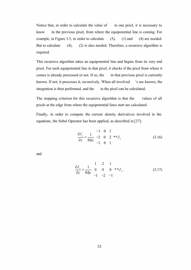
Finally, in order to compute the current density derivatives involved in the

equations, the Sobel Operator has been applied, as described in [27]:

1 0 11

2 0 28

1 0 1

yy

JJ

x x

− ∂ = − ∗∗ ∂ ∆

−

(3.16)

and

1 2 11

0 0 08

1 2 1

xx

JJ

y y

∂ = ∗∗ ∂ ∆

− − −

. (3.17)

33

3.3 Reconstruction by Integration along Cartesian Grid

Lines

In order to simplify the previous algorithm, the integration along a Cartesian grid

may be preferred.

Ider et al [15] claim that, if the gradient of the logarithmic resistivity ℜ is

known within the subject Ω , then ℜ can be found by integrating its gradient

along Cartesian grid lines, except for an additive constant. This is equivalent to

specifying the potential function at a single point in Ω .

The gradient of ℜ cannot be found for a single injected current profile, since the

determinant of the coefficient matrix in Equation (3.2) is zero. Let 1Jr

and 2Jr

be

the current density measurements, corresponding to two different applied

injection patterns. Then, within the imaging slice in xy plane, the third row of

Equation (3.2) can be written twice to obtain:

11

1 1

2 2 22

yx

y x

y x yx

JJJ J y xxJ J JJ

y y x

∂∂∂ℜ − − ∂ ∂∂ = ∂ℜ− ∂ ∂ − ∂ ∂ ∂

. (3.18)

From this new set of equations, it is possible to calculate the gradient of ℜ

T

x y ∂ℜ ∂ℜ ∂ ∂

at any point, provided that for that point the determinant

1 2 2 1y x y xJ J J J− + is not zero, or equivalently:

1 2 0xy xyJ J× ≠r r

, (3.19)

where 1xyJ

r and 2

xyJr

are the projections of 1Jr

and 2Jr

, respectively, on the xy

plane.

After finding the gradient of ℜ , using the first or second row of Equation (3.2),

it is possible to obtain z∂ℜ ∂ if at least one of the conditions ( 1 0yJ ≠ or 2 0yJ ≠ )

34

or ( 1 0xJ ≠ or 2 0xJ ≠ ) is satisfied, respectively. Since the condition in Equation

(3.19) is already required, one of those two conditions will hold anyway.

Handling the rows of Equation (3.2) in different orders, it can be seen that to find

the gradient of ℜ at any point, it is also sufficient to have ( )1 2 0xz xzJ J× ≠ or

( )1 2 0yz yzJ J× ≠ at that point.

In general, if

1 2 1 2 1 2 1 2 0yz yz xz xz xy xyJ J J J J J J J× = × + × + × ≠ (3.20)

at a certain point, then the gradient at that point can be calculated, because at

least one of the terms in Equation (3.20) will not vanish [15]. In practice, it may

be needed to employ more than two injection patterns, because the condition in

(3.20) may not be satisfied at all points by a single pair of injection patterns.

Note that by finding T

x y ∂ℜ ∂ℜ ∂ ∂

for only one xy plane, ℜ can only be

reconstructed at that plane, i.e. slice, apart from an additive constant, without

being concerned about finding the gradient at other xy slices. Similarly, this

occurs for xz and yz slices.

3.3.1 Implementation

In order to obtain the gradient of ℜ from the Equation (3.18), it is necessary to

calculate firstly:

1 1

2 2y x

y x

J JJ J

− −

(3.21)

and

11

22

yx

yx

JJy x

JJy x

∂∂−

∂ ∂ ∂∂ −

∂ ∂

. (3.22)

35

The derivatives of Equation (3.22) have been found by applying the Sobel

Operator [27] given in Equation (3.16) and Equation (3.17).

After obtaining the gradient of ℜ , the actual distribution of ℜ in every pixel can

be obtained by integration, using the methods explained previously in Section

3.2.1.2.

3.4 Reconstruction by Solution of a Linear Equation

System using Finite Differences

Ider et al [15] state that any row of Equation (3.2) can be discretized by using

finite differences on a rectangular mesh. For example, for a slice placed on the xy

plane, the third row of Equation (3.2) is chosen. This discretization is done for

each node within the slice and for every current injection pattern. A matrix

equation can be built by combining all the equations involved in the

discretization. Then, the logarithmic resistivity ℜ can be found with a matrix

inversion.

3.4.1 Algorithm

Let the slice image be on the xy plane. Then, the third row of Equation (3.2),

which was:

y xy x

J JJ J

x y x y

∂ ∂∂ℜ ∂ℜ− = − − ∂ ∂ ∂ ∂

(3.23)

can be discretized on a N N× Cartesian grid, by using finite differences [33].

Each pixel in the image holds the logarithmic resistivity ℜ at their center point.

There are three types of subsqueres: interior pixels, boundary pixels and corner

pixels, which correspond with nine different cases. In the next Section 3.4.2,

expressions for all of them will be given.

For example, for the inner points, central differences can be applied to Equation

(3.23) in order to approximate the derivatives in x and y direction. The result is:

36

( ) ( )( )

( ) ( )( )

( ) ( ) ( ) ( )

1, 1, , 1 , 1, ,

1, 1, , 1 , 1

2 2

,2 2

i j i j i j i jy i j x i j

y i j y i j x i j x i j

J Jx y

J J J J

x y

+ − + −

+ − + −

ℜ − ℜ ℜ − ℜ−

∆ ∆

− − = − − ∆ ∆

(3.24)

where x∆ and y∆ are the discretization steps in x and y directions, respectively,

and i and j are the indices of the center of the pixels in x and y directions,

respectively. For the rest of cases, backward, forward or central differences are

applied.

Once all the pixel elements are discretized, rearranging the set of finite difference

equations, the following linear system is obtained:

CR = B , (3.25)

where C is a 2 2N N× matrix containing the coefficient of ℜ in the left-hand

side part of Equation (3.24), 20 2 1

T

N − = ℜ ℜ ℜ R L is the logarithmic

resistivity distribution of the slice in vector form, and B are the current density

terms on the right-hand side of Equation (3.24).

If M different injected current patterns are carried out, the coefficient matrix C

and the right-hand side vectors B can be concatenated in order to obtain the

following set of equations:

1 1

22

MM

=

C B

BCR

BC

uux

MM. (3.26)

At least two injection patterns must be performed in order to satisfy the condition

given previously in Equation (3.20).

3.4.2 Implementation

Let the square target imaging region ( ) ( ): , ,S L L L LΩ − × − be uniformly divided

into N N× axis-parallel sub squares i jN+Ω , containing the logarithmic resistivity

37

ℜ values of the image at their center point ( ),i jx y , where 0, , 1i N= −K and

0, , 1j N= −K . The logarithmic resistivity ℜ is assumed to be constant on each

subsquare kΩ , denoted by kℜ , where 21, ,k N= K . As it was stated before, there

are three types of subsquares: in the interior, on the boundaries, and the corners.

The nine different cases can be shown in Figure 5.12(b). Expressions for each of

these cases are given below.

(a) (b)

Figure 3.6: Reconstruction by solution of a linear equation system. (a) kℜ ,

,x kJ and ,y kJ at every element kΩ and surrounding elements. (b) In the implementation, nine different types of elements are considered.

Firstly, considering an inner element kΩ .

1 for 1 , 2k i jN i j N= + + ≤ ≤ − ,

Equation (3.23) can be discretized using central differences in x and y direction.

It becomes:

, ,, ,1 1

, 1 , 1, ,

2 2 2 2

,2 2

y k y kx k x kk N k N k k

y k y kx k N x k N

J JJ J

y y x xJ JJ J

y x

+ − + −

− +− +

ℜ − ℜ + ℜ − ℜ∆ ∆ ∆ ∆

−−= +

∆ ∆

(3.27)

38

where ,x kJ represents the conductivity density in x direction in the pixel k, and

x∆ and y∆ are the element length in x and y direction, respectively. In this case,

2 /x y L N∆ = ∆ = .

In order to obtain the expression for the upper boundary, i.e.:

1 for 1 2 and 0k i jN i N j= + + ≤ ≤ − = ,

central differences are taken for x direction, while only forward differences in y

direction. Then, the Equation (3.23) is approximated by:

, ,, ,1 1

, 1 , 1, ,

2 2

.2

y k y kx k x kk N k k k

y k y kx k x k N

J JJ J

y y x xJ JJ J

y x

+ + −

− ++

ℜ − ℜ + ℜ − ℜ∆ ∆ ∆ ∆

−−= +

∆ ∆

(3.28)

Similarly, for the lower boundary of the image, i.e.:

1 for 1 2 and 1k i jN i N j N= + + ≤ ≤ − = − ,

central differences are taken for x direction, and backward differences in y

direction. Then, the Equation (3.23) is approximated by:

, ,, ,1 1

, 1 , 1, ,

2 2

.2

y k y kx k x kk k N k k

y k y kx k N x k

J JJ J

y y x xJ JJ J

y x

− + −

− +−

ℜ − ℜ + ℜ − ℜ∆ ∆ ∆ ∆

−−= +

∆ ∆

(3.29)

Equivalent procedure can be used to obtain the left-hand side boundary:

1 for 0 and 1 2k i jN i j N= + + = ≤ ≤ − ,

by using central differences in y direction and forward in x direction. Equation

(3.23) becomes:

, ,, ,1

, , 1, ,

2 2

.2

y k y kx k x kk N k N k k

y k y kx k N x k N

J JJ J

y y x xJ JJ J

y x

+ − +

+− +

ℜ − ℜ + ℜ − ℜ∆ ∆ ∆ ∆

−−= +

∆ ∆

(3.30)

39

For the right-hand side boundary elements, such that,

1 for 1 and 1 2k i jN i N j N= + + = − ≤ ≤ − ,

Equation (3.23) is approximated by backward differences in x direction and

central differences in y direction, resulting:

, ,, ,1

, 1 ,, ,

2 2

.2

y k y kx k x kk N k N k k

y k y kx k N x k N

J JJ J

y y x xJ JJ J

y x

+ − −

−− +

ℜ − ℜ + ℜ − ℜ∆ ∆ ∆ ∆

−−= +

∆ ∆

(3.31)

Finally, for the four corner elements, such that

1 for , 0 or 1k i jN i j N= + + = −

forward or backward differences are used. The expression for the upper-left one,

where 1k = , becomes:

, ,, ,1

, , 1, , .

y k y kx k x kk N k k

y k y kx k x k N

J JJ Jy y x x

J JJ Jy x

+ +

++

ℜ − + ℜ + ℜ ∆ ∆ ∆ ∆

−−= +

∆ ∆

(3.32)

In case of the upper-right corner, with k N= , it results:

, ,, ,1

, 1 ,, , .

y k y kx k x kk N k k

y k y kx k x k N

J JJ Jy x y x

J JJ Jy x

+ −

−+

ℜ + − ℜ − ℜ ∆ ∆ ∆ ∆

−−= +

∆ ∆

(3.33)

For the lower- left corner, where ( 1) 1k N N= − + , it yields:

, ,, ,1

, , 1, , .

y k y kx k x kk N k k

y k y kx k N x k

J JJ Jy y x x

J JJ Jy x

− +

+−

− ℜ + − ℜ + ℜ ∆ ∆ ∆ ∆

−−= +

∆ ∆

(3.34)

40

And, finally, the expression for the lower-right corner, where 2k N= , the

Equation (3.23) is approximated by:

, ,, ,1

, 1 ,, , .

y k y kx k x kk N k k

y k y kx k N x k

J JJ Jy x y x

J JJ Jy x

− −

−−

− ℜ + + ℜ − ℜ ∆ ∆ ∆ ∆

−−= +

∆ ∆

(3.35)

As previous ly stated, rearranging the terms in Equations (3.27) to (3.35) and

combining them, the matrix equation (3.25) can be formed. In the current

implementation of this algorithm, two orthogonal injection patterns have been

used. Therefore, this procedure has been repeated twice. Concatenating the C and

B matrices for each injection profile, the following matrix equation results:

1 1

2 2

C BR =

C B (3.36)

The rank of the combined C matrix is 2 1N − , as expected, since a function can be

reconstructed from its gradient, except for an additional constant [15]. It is

necessary to set one of the ℜ ’s to its real value and then solve the equation

system with full rank, in order to obtain the logarithmic resistivity ℜ in the slice.

For example, in order to set 0ℜ to its true value 0realℜ , then the first row of C1

must be changed, such that its element 0,0 1c = , while the rest 0, 0kc = for all

21, , 1k N= −K . Also, the element 0b of B1 must be set to 0 0realb = ℜ . Now, the

matrix is full rank and the system can be solved in order to get the true ℜ .

The linear system (3.36) has been solved by using the preconjugate gradient

method. This requires that the coefficient matrix C must be symmetric and

positive definite. In order to do that, C is multiplied by its transpose. Hence, the

actual linear system to be solved becomes:

T T T T

1 1

1 2 1 22 2

C BC C R = C C

C B, (3.37)

where T1C and T

2C are the transposes of 1C and 2C , respectively.

41

This method has been preferred to an SVD decomposition of C, due to the

dimension of C matrix, and its faster convergence and less demand of memory.

3.5 Reconstruction with Equipotential – Projection

Algorithm

In this section, the algorithm proposed in 1999 by Eyüboglu US patent [8] and

applied to real data by Özdemir [25], is extended. In this case, it can reconstruct a

relative conductivity distribution in a two dimensional slice without any potential

measurement. In order to obtain the true distribution, the potential at one element

on the boundary must be known.

3.5.1 Algorithm

The current density distribution Jr

is obtained using MRI from the magnetic flux

density distribution, as described in Section 2.4, while current is injected to the

subject through electrodes attached to its boundary. Equipotential lines inside the

subject can be determined by calculating the orthogonal lines to the current

density Jr

paths.

At this point, assuming that the conductivity is uniform and known for a column

of the FOV, it is possible to calculate by Ohm’s law the gradient of the potential

for every element in that column.

J

φσ

∇ = −r

(3.38)

The potential distribution φ in the column is obtained by integration of this

gradient φ∇ . If a voltage measurement is performed on this boundary column,

the potential values will be true and, therefore, the final conductivity distribution

will be absolute. If no voltage is measured, on the contrary, a relative

conductivity distribution will result.

Once the potential is calculated in the column, it is projected throughout the FOV

by using the equipotential lines. Then, the gradient of the potential distribution

42

φ∇ in the whole FOV is calculated. Finally, using again Ohm’s law, Equation

(3.38), the conductivity distribution is found.

Note that if the conductivity of the column is known, the reconstructed

conductivity values will be true conductivities.

3.5.2 Implementation

In this section, some aspects about the implementation of the algorithm are

explained.

The gradients are calculated by the Sobel operators, given in Equation (3.16) and

Equation (3.17).

The equipotential lines are found by using the procedure described previously in

Section 3.2.1.1. Once they are obtained, the potential values at the boundary are

projected inside of the domain following these paths. Thus, the potential assigned

to each pixel is a weighted average of all the potential values that the crossing

equipotential lines carry and their length within the pixel. In a more formal

manner, the potential for the ith pixel, iφ , crossed by eqLN equipotential lines is

calculated as:

1

1

eqL

j

eqL

N

j eqLj

i N

jj

l

l

φφ =

=

=∑

∑, (3.39)

where jeqLφ is the potential which the jth equipotential line inside the pixel

carries, and jl is its length within the pixel.

43

3.6 Reconstruction with J-substitution Algorithm

Kwon et al [20] proposed a new static resistivity image reconstruction algorithm,

called J-substitution, and presented simulation results in 2002. They declared the

image reconstruction as a constructive map , ,I J V ρ→ inside a region Ω

within the subject, where I is the injected current, J is the magnitude of the

current density and V is the peripheral voltage measurements. They assumed that

the magnitude of the internal current density distribution is available from an

MRI system, including the supplementary current injections added to the subject.

3.6.1 Problem Definition

Let Ω denote a two-dimensional cross section of an electrically conducting

body, with resistivity distribution, denoted by *ρ . The resistivity distribution *ρ

in the region Ω and the voltage *Vρ

are unknown, but the magnitude of the

current density, *Jr

, is known by using MRI. Injection currents I through

electrodes attached on the boundary ∂Ω are also included in the given current

density image. These injected currents I generate current densities on the

boundary ∂Ω , whose inward pointing normal components, denoted by Ij ,

satisfy the compatibility condition:

0Ij ds∂Ω

=∫ .

The inverse problem, then, is to reconstruct the resistivity distribution *ρ from

the known ( )*,I J pair data, using the physical laws of electromagnetics.

The nonlinear relation between the resistivity distribution ρ , and the

corresponding potential field Vρ is given by the boundary value problem (BVP)

defined by the following Poisson’s relation, together with Neumann boundary

conditions:

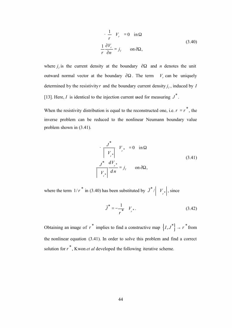
44

1· 0 in

1on ,I

V

Vj

n

ρ

ρ

ρ

ρ

∇ ∇ = Ω

∂ = ∂Ω ∂

(3.40)

where Ij is the current density at the boundary ∂Ω and n denotes the unit

outward normal vector at the boundary ∂Ω . The term Vρ∇ can be uniquely

determined by the resistivity ρ and the boundary current density Ij , induced by I

[13]. Here, I is identical to the injection current used for measuring *J .

When the resistivity distribution is equal to the reconstructed one, i.e. *ρ ρ= , the

inverse problem can be reduced to the nonlinear Neumann boundary value

problem shown in (3.41).

*

*

*

*

*

*

· 0 in

on ,I

JV

V

VJj

nV

ρ

ρ

ρ

ρ

δ

δ

∇ ∇ = Ω

∇ = ∂Ω ∇

(3.41)

where the term *1/ ρ in (3.40) has been substituted by ** /J V

ρ∇

r, since

**

*1

J Vρρ

= − ∇r

. (3.42)

Obtaining an image of *ρ implies to find a constructive map * *,I J ρ→ from

the nonlinear equation (3.41). In order to solve this problem and find a correct

solution for *ρ , Kwon et al developed the following iterative scheme.

45

3.6.2 Algorithm

In their iterative algorithm, they minimize the cost function ( )ρΦ , such that:

( ) ( ) ( ) ( )2

* 1: J r E r dr

r ρρρ

Ω

Φ = −∫ r r rr , (3.43)

where ( )*J rr

is the magnitude of the observed interior current density and

( ) ( ):E r V rρ ρ= ∇r r is the magnitude of the calculated electric field intensity

obtained by solving (3.41) for a given ρ .

They also established that if at least two currents, 1I and 2I satisfying the

following condition:

1 2 0J J× ≠ (3.44)

are applied, together with a single voltage measurement, the true conductivity

image can be reconstructed.

In this thesis, two opposite orthogonal pairs of electrodes are used. Hence, two

current patterns are applied.

Let 1I and 2I be the two currents injected via two pairs of electrodes. Then, two

sets of current density data, 1 1J J=r

and 2 2J J=r

, induced by 1I and 2I ,

respectively, are used to image the resistivity distribution. The position of the

electrodes makes 1J and 2J satisfy the condition (3.44).

The J-substitution reconstruction algorithm solves the nonlinear problem

described in (3.41), determining *ρ from two pairs of data ( ),q qI J , where

1,2q = is the injection pattern number. The steps of this iterative algorithm are

the following:

46

• Initial guess: For the initial guess, a homogeneous resistivity 0ρ is

chosen. For example, 0 1ρ = .

• Forward solver: For a given resistivity 2 p qρ + , where 1,2q = indicates the

injection pattern and 0,1,2,p = K the iteration number, the forward

problem is given by

2

2

1· 0 in

1on and 0.q

qpp q

qp q

pp q I

V

Vj V ds

n

ρ

δ

ρ δ

+

+∂Ω

∇ ∇ = Ω

= ∂Ω =

∫ (3.45)

In this implementation, the Cell-Centered Finite Difference Method [19]

has been used, similarly as [20]. Implementation of this method was

described in the Section 2.2.3.

• Update 2 1p qρ + + . Since ρ and αρ , where α is a positive constant, will

induce the same current density distribution J , but the corresponding

voltages are actually scaled by α , the absolute resistivity value needs to

be calculated by updating the resistivity using a voltage measurement, as

follows:

2

2 1 *:

p q

qqpp q

q q

fV

J fρ

ρ

ρ+

+ +∇

= , (3.46)

where *qf

ρ is the measured voltage difference between two current

injection electrodes for the injection current qI , and 2 p qqf

ρ + is the

calculated voltage difference when the resistivity distribution is given by

computed 2 p qρ + .

• If 2 1 2p q p qρ ρ ε+ + +− < , for a precision error ε , stop. Otherwise, go back

to Step 2) with 1q q= + when 1q = , or with 1p p= + and 1q = if

2q = , where q is the injection pattern and p is the iteration number.

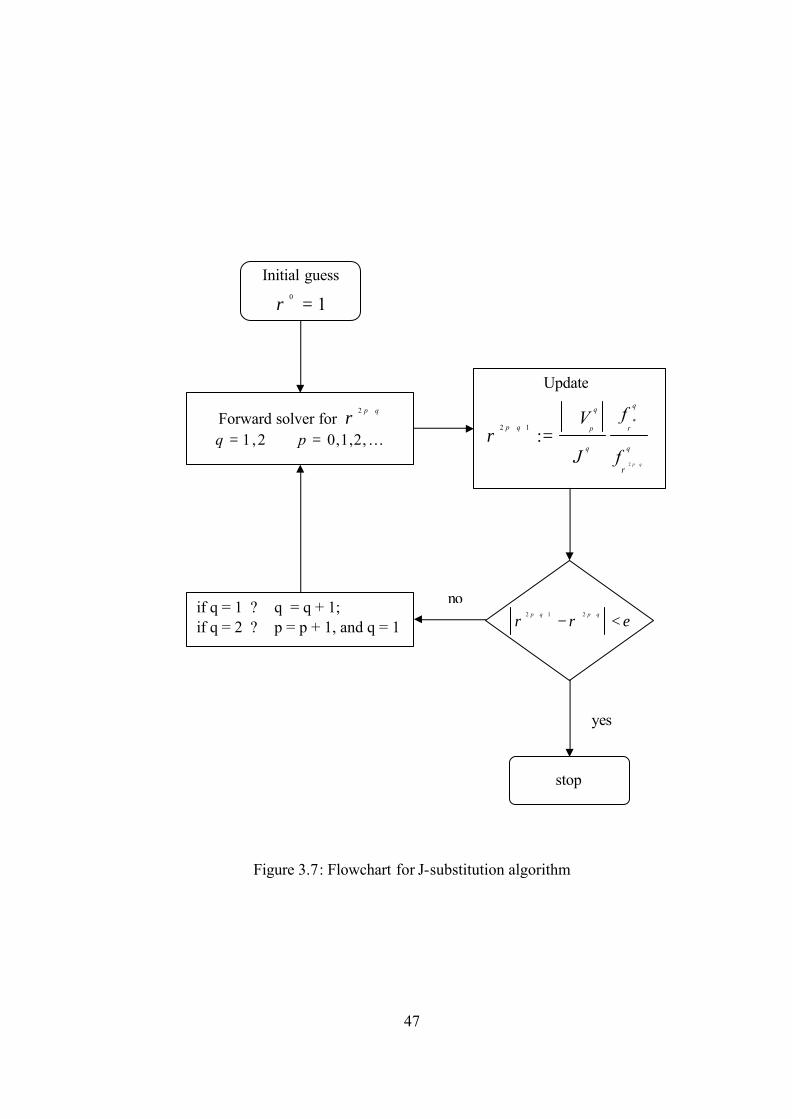
47

Figure 3.7: Flowchart for J-substitution algorithm

Initial guess 0 1ρ =

Forward solver for 2 p qρ +

1,2q = 0,1,2,p = K

if q = 1 ? q = q + 1; if q = 2 ? p = p + 1, and q = 1

Update

2

*2 1

:p q

qq

p q p

q q

fV

J f

ρ

ρ

ρ+

+ +∇

=

2 1 2p q p q

ρ ρ ε+ + +

− <

stop

no

yes

48

CHAPTER 4

MAGNETIC FLUX DENSITY BASED

RECONSTRUCTION ALGORITHM

4.1 Introduction

The harmonic zB reconstruction algorithm studied next belongs to the second

family of algorithms described in the Section 2.4.3.

Seo et al [30] in 2003 proposed a new algorithm, where one single component of

the induced magnetic flux density, zB , is measured using an MRI scanner

without rotating the object. It is based on the computation of 2zB∇ as shown

previously in (2.64), so the noisy zB is differentiated twice.

Oh et al [22], also in 2003, improves this technique with the harmonic

zB algorithm. Here, they use a layer potential technique [16] in two dimensions

to recover σ from σ∇ , instead of line integrals, as Seo et al [30] suggested

firstly, since they tend to accumulate errors.

4.2 Problem Definition

Oh et al [22] places a subject Ω into an MRI scanner, while ζ surface

electrodes are attached on its boundary in order to inject current. Each current

injection pattern can be performed by using two of those electrodes. Therefore,

the possible number of different injection patterns using ζ electrodes is

( 1 ) /2N ζ ζ= − , [22]. Let the injection current between the jth pair of electrodes

49

be jI for 1, ,j N= K . This current produces a current density ( ), ,j j j jx y zJ J J J=

r

inside the subject. The presence of the internal current density jJr

and the current jI in the lead wires generate a magnetic flux density ( ), ,j j j j

x y zB B B B=r

, so that

0j jB Jµ∇× =

r rholds inside the electrically conducting subject. This induced

magnetic flux density causes an increment in the MR phase image, proportional

to the B component in the direction parallel to the main magnetic field. If this is

placed in z-direction, the jzB components, from 1, ,j N= K , are assumed to have

been obtained from the corresponding MR phase images of the subject.

The subject has an isotropic conductivity distribution σ , such that 0 σ< < ∞ .

Let ju be the voltage due to the injection current jI for 1, ,j N= K . Since σ is

approximately independent of injection currents, each ju is a solution of the

following Neumann boundary problem:

( )· 0 in

ˆ· on ,

j

j j

u

u n g

σ

σ

∇ ∇ = Ω

− ∇ = ∂Ω (4.1)

where n is the outward unit normal vector and jg is the normal component of

current density on the boundary ∂Ω for the injection current jI . Across a current

injection electrode ζ ,

j jg ds Iζ

= ±∫ ,

where the sign depends on the direction of current, and jg is zero on the regions

of the boundary which are not in contact with the current injection electrodes

used for the jth injection pattern.

If the conductivity distribution σ , applied current jI and electrode configuration

are given, the boundary problem (4.1) can be solved for ju by using numerical

methods, such as the finite element method (FEM). But, for this algorithm, the

cell-centered finite difference method, explained in the Section 2.2.3, is used.

50

From the z-component of the relation of 20B uµ σ∇ = − ∇ ×∇

robserved by [27],

and previously introduced in (2.64), the expression (4.2) can be obtained for each

position inside the subject and each injection pattern 1, ,j N= K .

2

0

1, · , 1, ,

j jj

z

u uB j N

x y y xσ σ

µ ∂ ∂ ∂ ∂

∇ = − = ∂ ∂ ∂ ∂ K . (4.2)

Using a matrix notation, (4.2) can be written as:

U s = b , (4.3)

where

1 1

2 1

0 2

1and

z

NN Nz

u uBy x

x

Bu u yy x

σ

σ µ

∂ ∂− ∂ ∇∂ ∂ ∂ = = = ∂ ∇∂ ∂ ∂− ∂ ∂

U s bM M M . (4.4)

In this implementation, two injection currents are used ( 2N = ).

In order to solve (4.3), U must be invertible, that is, the determinant of U must be

non-zero. The two current densities 1Jr

and 2Jr

must be chosen so that 1I and 2I satisfy:

1 2 1 2 0x y y xJ J J J− = . (4.5)

This implies that the two current densities are not collinear inside the subject

[17], [15].

Using the weighted regularized least square method, s vector can be obtained as:

( )T Tλ-1

s = U U + I U b% % % % , (4.6)

where:

• =U WU% ,

• TU% is the transpose of U% ,

51

• λ is a positive regularization parameter. It is set to ( )1

det Tλ =

U U% %,

• I is the 2 2× identity matrix,

• b = W b% ,

• 1diag( , , )Nw w=W K is a N N× diagonal weight matrix. The weighting

factor jw are set to

1

jj N

jj

SNRw

SNR=

=

∑, (4.7)

where jSNR is the signal-to-noise-ratio (SNR) of the measured jzB . This

jSNR should be determined for each position of pixel, although it is

difficult in practice to know it. The way to estimate this jSNR is

explained in Section 4.4.

Then, calculating (4.6) for each pixel, the distribution of T

x yσ σ ∂ ∂

= ∂ ∂ s inside

the subject is obtained. The next step must be to recover the σ distribution.

Now, the imaging slice S is assumed to be lying in the plane 0z = and the

conductivity value is 1 at a fixed position 0 0 0( , ,0)r x y=r

on its boundary S∂ . In

order to simplify the following expressions, ( , )r x y=r , ' ( ', ')r x y=r and

( , ,0) ( )x y rσ σ= r . Oh et al [22] use a layer potential technique in two dimensions

in order to compute the σ distribution from ,x yσ σ

σ ∂ ∂

∇ = ∂ ∂ , instead of using

line integral, as Seo et al [30] suggested, since this latter technique accumulates

errors. Then,

2

' ' ' '

( ) ( ') ( ') '

ˆ( ')· ( ') ' · ( ') ( ') ,S

r r r rS S

r r r r dr

r r r dr n r r r dl

σ σ

σ σ∂

= ∇ Φ − =

= − ∇ Φ − ∇ + ∇ Φ −

∫∫ ∫r r r r

r r r r r

r r r r r r r (4.8)

52

where

' 2

1 1 '( ') log ' and ( ')

2 2 'r

r rr r r r r r

r rπ π−

Φ − = − ∇ Φ − = −−

r

r rr r r r r r

r r .

The second integral in (4.8) can be approximated by [1] for points such that

r S∈ ∂r

' ' ' ' ' '0

( )ˆ ˆ ˆlim · ( ') ( ') · ( ') ( ')2r r r r r r rS St

rn r tn r r dl n r r r dl

σσ σ

+ ∂ ∂→∇ Φ − − = + ∇ Φ −∫ ∫r r r r r r r

rr r r r r r

.

Therefore, as r S∈r

approaches the boundary S∂ , the equation (4.8) becomes:

( ) ( )'

'2 2

ˆ' · ' · ( ')( ) 1 1( ') '

2 2 2' 'r SS

S rS S

r r n r r rrr dl dr

r r r r

σσσ

π π∂∂

∂∂

− − ∇+ =

− −∫ ∫rr

r r r r rrr r

r r r r , (4.9)

where Sσ∂ denotes the conductivity restricted to the boundary S∂ . Since σ∇ is

known in S, the right-hand side of (4.9) is known. Then, by [1], the equation

(4.9) is guaranteed to be solved and the Sσ∂ can be found. Now, this Sσ∂ can be

substituted in (4.8), in order to obtain σ in S as follows:

' ' ' '

' '2 2

ˆ( ) ( ')· ( ') ' · ( ') ( ')

1 ( ') 1 ( ')ˆ( ') ' · ( ') .2 2' '

r r r S rS S

r S rS S

r r r r dr n r r r dl

r r r rr dr n r dl

r r r r

σ σ σ

σ σπ π

∂∂

∂∂

= − ∇ Φ − ∇ + ∇ Φ − =

− −= ∇ −

− −

∫ ∫

∫ ∫r r r r

r r

r r r r r r r r

r r r rr r r

r r r r (4.10)

This process of solving (4.6) for each pixel, and (4.9) and (4.10) for each

imaging slice can be repeated for all imaging slices of interest within the subject,

as long as the measured data zB are available for the slices.

4.3 Algorithm

Since, in order to solve (4.1) the true conductivity distribution σ is unknown and

in order to obtain this σ , the matrix U with u∇ in (4.3) is needed, as well.

Therefore, an iterative algorithm is required.

The injection currents jI are applied through a given pair of electrodes and the z-

component of the induced magnetic flux density jzB is measured for each

53

imaging slice. Also, the boundary voltages j

Su

∂on the electrodes which are not

injecting the current jI are measured.

Then, the 2zB∇ iterative algorithm has the following steps:

Step 1. Let 0m = and assume an initial conductivity distribution 0σ .

Step 2. Calculate 1j

mu + by solving the following Neumann boundary

problem for each 1, ,j N= K :

( )1

1

· 0 in

ˆ· on .

jm m

j jm m

u

u n g

σ

σ+

+

∇ ∇ = Ω

− ∇ = ∂Ω (4.11)

Step 3. Calculate 1mσ + using (4.6), (4.9) and (4.10). Scale 1mσ + using the

measured boundary voltages j

Su

∂and the calculated ones 1

jm S

u + ∂.

Step 4. If 1

1

m m

m

σ σε

σ+

+

−< for a given tolerance ε , continue with Step 5).

Otherwise, set ( 1)m m= + and go back to Step 2).

Step 5. Calculate the current density image as 1j j

m MJ uσ += − ∇r

, where

jMu is a solution of the boundary value problem in (4.1), with σ replaced

by 1mσ + .

4.4 Implementation

In order to compute the b matrix, in (4.4) the term 2zB∇ is needed for every pixel.

The 2zB∇ at the ith pixel can be calculated with the following three-point

difference scheme:

54

( ) ( ) ( ) ( )( )

( ) ( ) ( )( )

( ) ( ) ( )( )

1 122

1 12

1 12

, , 2 , , , ,, ,

, , 2 , , , ,

, , 2 , , , ,,

z i i i z i i i z i i iz i i i

z i i i z i i i z i i i

z i i i z i i i z i i i

B x y z B x y z B x y zB x y z

x

B x y z B x y z B x y z

y

B x y z B x y z B x y z

z

+ −

+ −

+ −

− +∇ = +

∆

− ++ +

∆

− ++

∆

(4.12)

where x∆ , y∆ and z∆ are the distances between adjacent pixels in the x-, y- and

z-directions, respectively.

Consequently, the induced zB field is needed for every pixel within the slice to be

imaged, and in an upper and lower imaginary planes, out of the slice. In the

implementation of the algorithm, these two outer planes are placed at 0.83 mm

from the real slice.

In this thesis, the forward solver actually provides current density as simulation

data. Therefore, for each injection current jI , the z-component of the induced

magnetic flux density jzB for 1, ,j N= K can be approximated as a matrix

equation, by discretizing the Biot-Savart law. This procedure was explained in

the Section 2.2.4.

Hence, by using the equation (2.45), zB can be calculated as:

z x yB J J= −y xD D . (4.13)

Now, using (4.12), 2zB∇ is obtained for every element in the slice, so the b

matrix can be calculated and (4.3) can be finally solved.

55

Figure 4.1: Flowchart for Harmonic Bz algorithm

Forward solver for 1

j

mu

+

1,2j =

Update and scale

1mσ

+

m = m + 1 2 1 2p q p q

ρ ρ ε+ + +

− <

Initial guess 0 1ρ =

stop

no

yes

56

CHAPTER 5

SIMULATION AND COMPARISON

5.1 Introduction

This chapter is reserved for the simulation results and comparison of the

reconstruction algorithms described previously. This analysis covers different

cases, with and without noise, different techniques for the same algorithm, or

different stopping criteria for iterative algorithms.

5.2 Conductivity models

Two different two-dimensional conductivity models have been used to illustrate

the performance of the reconstruction methods described in previous chapters.

One of them was previously used to collect experimental data, while the other

has been defined to provide simulated data to the reconstruction algorithms

studied in this thesis.

In order to decide the dimensions of the simulated conductivity model and

amount of injected current, several previous studies have been considered. It has

been observed that reconstruction algorithms in noise-free cases are not affected

by the amount of current applied. The absolute values of the simulated data

change but, since the proportions between conductivity, current density and

potential are kept, the reconstructed image remains the same. Ider et al [15]

considered 100 mA for noisy cases and a phantom of 20 20× cm. Oh et al [22]

used 26 mA for an object of 50 50× mm. Özbek [24] and Birgül [2] collected

measured data in the 0.15 Tesla METU-EE MRI system, using 20 mA for an

57

experimental phantom of 6 6 cm× . In order to compare all the reconstruction

algorithms under the same conditions and be consistent with the experimental

data of [24] and [2], which has been also used as the experimental phantom, the

size of the imaging slice has been finally chosen as 6 6 cm× , and the total

injected current has been established in 20 mA for each injection pattern.

5.2.1 Simulated phantom

Figure 5.1(a) shows the geometry of an electrically conducting phantom with an

isotropic and piecewise constant conductivity distribution σ . The dimensions of

this numerical phantom is 6 6 cm× , discretized into 50 50× square elements.

Assigned conductivity values for the regions of the phantom are listed in Table

5.1. The background conductivity (3) has been chosen to be 2 S/m, which is

close to the average body conductivity. There are two different conductivity

perturbations in it: a rectangle (1) and a circle (2). The rectangle is more

conductive than the background, with conductivity equal to 4 S/m, while the

circle is more resistive, with conductivity set to 1 S/m.

The currents are injected using four constant-current electrodes, covering the

whole sides, as shown in Figure 5.1(b). Therefore, two different and orthogonal

injection patterns are possible for the two pairs of electrodes. A total injected

current of 20 mA has been used for each injection pattern.

Table 5.1: Simulated conductivity model values

Region Object Conductivity value (S/m)

1 Rectangle 4 2 Circle 1 3 Background 2

58

(a)

(b) (c)

(d) (e)

Figure 5.1: Definition for the simulated conductivity model. (a) Regions of different conductivity. The conductivity values are given in Table 5.1. Position of current electrodes for orthogonal injection patterns 1 (b) and 2 (d). Total current density distribution for injection pattern 1 (c) and 2 (e).

59

x

y

z 1

2

5.2.2 Experimental phantom

The geometry of the experimental phantom can be seen in Figure 5.2. This test

phantom is 6 6 2 cm× × , discretized into 30 30× square elements. It is filled with

Agar gel, with conductivity 2 S/m. Since the third dimension is small enough

compared with the other two dimensions, the applied current is assumed to flow

only in the x-y plane and the problem can be simplified to a two-dimensional

one. A conductor object of 2.5 2.5 2 cm× × , with conductivity 9 S/m is placed in

the center. The currents are injected using four small electrodes, opposite to each

other. Thus, two orthogonal injection patters can be performed, with a total

injected current of 20 mA for each case.

Table 5.2: Experimental conductivity model values

Region Object Conductivity value (S/m)

1 Square 9 2 Background 2

Figure 5.2: Definition for the experimental conductivity model. The regions of different conductivity and electrode positions are shown [24]. The conductivity values are given in Table 5.2.

60

5.3 Simulation of measurement noise

In order to compare the performance of the algorithms in presence of noise, the

random Gaussian noise model explained by Scott et al [28], and reviewed in

APPENDIX A is used. In their model, the noise is induced as a MR phase error,

independent of the magnetic flux density and, therefore, of the injected current.

Thus, if the amount of injected current is increased, the induced magnetic flux is

increased, so the proportional noise in magnetic flux density is reduced.

However, in [15], 10% of the magnitude of each current density component and

injection is multiplied by a random number in the range of 1± and added to the

corresponding noise-free current density. But, the model of Scott et al [28] is

more realistic; since the noise is independent of the direction of the current

injection and independent of its magnitude. It only depends on the MRI system

where the experiments are carried out. The reconstructed algorithms are tested

using different noise levels, corresponding to SNR equal to 60, 30 and 20. For

each level, the maximum noise included in the current density data with respect

to the maximum value of the noise-free case, is given in Table 5.3.

Table 5.3: Maximum noise level in xJ and yJ with respect to the maximum currents densities for the different noise levels

Injection pattern 1 Injection pattern 2 xJ yJ xJ yJ

SNR 60 14.8% 5.2% 5.1% 19.7% SNR 30 33.5% 11.5% 11.6% 43.1% SNR 20 43.6% 16.5% 15.1% 61.9%

One noise experiment is performed for each SNR and the resulting noisy current

densities are fed to the algorithms. This ensures that all algorithms run under the

same conditions, since different experiments can affect different pixels and

provoke different behaviors.

61

5.4 Error calculation and stopping criteria

In order to evaluate performance of the studied algorithms, error in the

reconstructed conductivity is calculated. In practice, the real conductivity is not

known a priori, but in this thesis, since the algorithms are fed with simulated

data, the true conductivity distribution is actually known.

The total error committed at reconstructing the whole image Tσε is calculated as:

100%t rT

tσ

σ σε

σ−

= × , (4.14)

where tσ and rσ are the true and reconstructed conductivity distributions,

respectively, and · is the 2L norm, defined as:

1 2

2i

i

a a

= ∑r

, (4.15)

where ia is the ith element of ar

.

The conductivity error of a reconstructed region in the image is calculated with

Equation (4.14), but restricted to the desired zone, resulting:

, ,,

,

100%t region rregionregion

t regionσ

σ σε

σ

−= × , (4.16)

where, ,tregionσ and ,rregionσ are the true and reconstructed conductivity

distributions for that conductivity region, respectively.

In order to end the iterative algorithms, different types of stopping criteria are

defined. In real cases, the true conductivity distribution is unknown. Therefore, a

stopping criterion based on the difference ,mσε between the reconstructed

conductivity of two successive iterations is used:

1,

m mm

mσ

σ σε

σ−−

= , (4.17)

62

where m is the iteration number and · is the 2L norm previously defined in

(4.15). As the iterations run, ,mσε decreases monotonically for noise-free cases.

Thus, if ,mσε ε< , for a given tolerance ε , the algorithm is said to have

converged to the actual values of conductivity distribution.

In noisy cases, the convergence function can reach a minimum, but greater than

the tolerance ε , and increase again. Then, a maximum number of iterations is

needed as stopping criteria. Then, the reconstructed conductivity distribution is

chosen as the one where the difference between iterations ,mσε is minimum.

In case of simulated data, the true distribution is known. Then, running a fixed

number of iterations, the convergence function can be studied and the

conductivity distribution with minimum total error Tσε with respect to the true

distribution is chosen.

5.5 Spatial Resolution

Spatial resolution describes the minimum size an object must be to be seen in an

image [31]. It also describes the degree of deblurring present in an image. It is

often represented by: Point Spread Function (PSF), Line Spread Function (LSF)

and edge response, Modulation Transfer Function (MTF) or System Transfer

Function (STF).

The PSF contains complete information about the spatial resolution. To express

the spatial resolution by a single number, it is possible to ignore the shape of the

PSF and simply measure its width. The most common way to specify this is by

the Full-Width-at-Half-Maximum (FWHM) value. Unfortunately, this method

has two significant drawbacks. First, it does not match other measures of spatial

resolution, including the subjective judgment of observers viewing the images.

Second, it is usually very difficult to directly measure the PSF.

63

Figure 5.3: Line spread function (LSF) and edge response [31].

As it is shown in Figure 5.3, the LSF is the response of the system to a thin line

across the image. Similarly, the edge response is how the system responds to a

sharp straight discontinuity, an edge. Since a line is the derivative of an edge, the

LSF is the derivative of the edge response. The width of the LSF is usually

spread as the FWHM, while the width of the edge response is normally quoted

by the 10% to 90% distance.

In this thesis, the Line Spread Function is used in order to quantify the blurring

effect of the reconstruction algorithms and different methods of integration. The

LSF is measured as the FWHM of the derivative of the edge response at the

edges of the rectangle in the phantom.

5.6 Simulation Results for Current Density Based

Algorithms

In the following sections, the results for the Type-I reconstruction algorithms,

explained in chapter 3, and based on current density, are given and discussed.

64

5.6.1 Reconstruction by Integration along Equipotential Lines

In this section, the resulting conductivity images using the reconstruction method

described in Section 3.2 are shown. The effects of the different integration

methods described in Section 3.2.1.2 and different noise levels are also

considered.

Firstly, the equipotential lines are calculated starting from the left edge of the

phantom, using the algorithm explained previously in Section 3.2.1.1. For this

purpose, the simulated current density, corresponding to the vertical injection

pattern, labeled as (1) in Figure 5.1(d) is used. Figure 5.4(b), shows the

calculated equipotential lines, when two of them begin from every pixel at the

left boundary. It can be seen that the equipotential lines get closer to each other

around the contours of the objects, while the upper and lower parts of the image

result uncovered. At an interface between two regions of different conductivity,

the currents tend to enter the more conductive one, but avoid the more isolator

one. Then, since the equipotential lines are orthogonal to the current streamlines

at every point, the equipotential lines bend, coming very close to each other,

accumulating around the circle contour and at the upper and lower edge of the

rectangle. Another side effect appears due to this reason. The current density is

assumed to be constant within a pixel. But, the pixel size may be too large in

those accumulation areas and contain, however, more than one current

streamline. This provokes that, during the calculation of the equipotential lines,

some paths cross others. This behavior is not valid, so the equipotential lines

involved are detected and removed. In the noise-free simulations carried out with

this phantom, around 2% of the total equipotential lines are invalid for this

reason. They are not taken into consideration for the integration in the

reconstruction, but provoke small errors, due to the information loss.

After the equipotential lines are found, current density derivatives are integrated

along these paths. If more than one equipotential line crosses a pixel, the ℜ

value assigned to the pixel is an average between the values calculated for each

equipotential line. The resistivity of the left column is assumed to be known.

65

The reconstructed images for the noise-free case can be seen in Figure 5.4, while

the errors committed at reconstructing each conductivity region and the total

image can be seen in Table 5.4.

Table 5.4: Errors in reconstruction along equipotential lines

Reconstructed Conductivity

Circle ( Circσε ) (%)

Rectangle ( Rectσε ) (%)

Background ( Bkcgσε ) (%)

Total error (%)

Trapezoidal integration method Noise free 3 equipot. lines 17.90 12.97 9.91 11.75 10 equipot. lines 17.69 12.15 9.74 11.36 Noisy cases. 10 equipot. lines SNR 60 18.38 14.92 10.14 12.59 SNR 30 28.50 17.36 19.09 20.18 SNR 20 25.23 25.65 20.12 23.30

Taylor Expansion method Noise free 3 equipot. lines 20.90 13.25 10.38 12.28 10 equipot. lines 20.61 12.54 10.23 11.94 Noisy cases. 10 equipot. lines SNR 60 20.74 15.26 10.47 13.02 SNR 30 28.67 17.53 19.31 20.40 SNR 20 25.84 25.44 20.37 23.43

The blurring effect of the different integration methods is studied next. As it was

explained previously in Section 5.5, the measurement of the spatial resolution by

calculating the width of the LSF at FWHM at one edge inside the image can

provide an idea of the degree of blurring of the reconstructed images. Figure 5.5

shows the horizontal profile and LSF images for a line crossing an edge of the

rectangle. The LSF widths for both trapezoidal integration method and Taylor

expansion method are given in Table 5.5.

Table 5.5: FWHM of LSF for reconstruction along equipotential lines

Reconstructed Conductivity

Trapezoidal integration FWHM (cm)

Taylor Expansion FWHM (cm)

Noise free 10 equipot. Lines 0.297 0.254

Noisy case. SNR 20 10 equipot. lines 0.200 0.230

66

[S·m-1]

0

0.5

1

1.5

2

2.5

3

3.5

4

-3 3-3

3

(a) (b)

(c) (d)

(e) (f)

Figure 5.4: Reconstruction by integration along equipotential lines. Noise-free cases. All the figures have the same gray scale. (a) True conductivity distribution. (b) Equipotential lines. 2 equipotential lines start for each pixel at the left edge. Reconstructed conductivity images, where 3 equipotential lines per pixel start from left boundary, using (c) Trapezoidal integration or (d) Taylor Expansion. Reconstructed conductivity images with 10 equipotential lines per pixel, using (e) Trapezoidal integration method or (f) Taylor Expansion.

67

As expected, the trapezoidal integration method produces wider LSF and,

therefore, more blurred contours. This is because it takes into consideration the

current density derivatives of the previous and current pixel. The Taylor

expansion method produces sharper objects, since it only integrates the current

density derivatives of the current pixel. As a disadvantage, the committed error in

the latter case is slightly larger.

In the reconstructed images, some horizontal artifacts in the direction of

integration, mainly horizontally, along the equipotential paths are due to the

accumulation of errors, typical of the integration techniques. This effect is more

important when less equipotential lines per pixel are started from the left

boundary. The pixels which are not crossed by any equipotential lines are

assigned to have zero conductivity and appear as the darkest regions. They are

not considered for the error calculation. This effect could be minimized tracing

equipotential lines from the right boundary, as well. But, even in those

conditions, the circle is too far from the lower electrode, and a big area under it,

with very little current, still remains. It would be necessary to include more

injection patterns to fill with information those areas, like horizontal or diagonal

ones.

Afterwards, different noise levels have been tested, equivalent to SNR equal to

60, 30 and 20. For the same noisy experiment, the image has been reconstructed

by both integration methods and compared. The conductivity errors are given in

Table 5.4, while the reconstructed images for trapezoidal integration method can

be seen in Figure 5.7. In all cases, ten equipotential lines are started from the left

column of the image. The blurring effects of the different integration methods are

studied in Figure 5.6, where the horizontal profile and LSF images for a line

crossing an edge of the rectangle are given, for case of SNR equal to 20.

68

(a)

-3 -2 -1 0 1 2 31.5

2

2.5

3

3.5

4

4.5

Position along x direction (cm)

Con

duct

ivity

(S

·m-1

)

-3 -2 -1 0 1 2 31.5

2

2.5

3

3.5

4

4.5

Position along x direction (cm)

Con

duct

ivity

(S

·m-1

)

(b) (c)

-2.8 -2.7 -2.6 -2.5 -2.4 -2.3 -2.2 -2.1 -2 -1.9 -1.8

0

0.5

1

Position along x direction (cm)

LSF

FWHM

-2.8 -2.7 -2.6 -2.5 -2.4 -2.3 -2.2 -2.1 -2 -1.9 -1.8

0

0.5

1

Position along x direction (cm)

LSF

FWHM

(d) (e)

Figure 5.5: Profile and LSF images for reconstruction by integration along equipotential lines. Noise-free cases. 10 equipotentia l lines per pixel. (a) True distribution. The dashed line gives the definition of the profile images. (b) Profile image for trapezoidal integration. (c) Profile image for Taylor expansion method. (d) LSF for trapezoidal integration. (e) LSF for Taylor expansion.

69

-3 -2 -1 0 1 2 30.5

1

1.5

2

2.5

3

3.5

4

4.5

Position along x direction (cm)

Con

duct

ivity

(S

·m-1

)

-3 -2 -1 0 1 2 30.5

1

1.5

2

2.5

3

3.5

4

4.5

Position along x direction (cm)

Con

duct

ivity

(S

·m-1

)

(a) (b)

-2.8 -2.7 -2.6 -2.5 -2.4 -2.3 -2.2 -2.1 -2 -1.9 -1.8

0

0.5

1

Position along x direction (cm)

LSF

FWHM

-2.8 -2.7 -2.6 -2.5 -2.4 -2.3 -2.2 -2.1 -2 -1.9 -1.8

0

0.5

1

Position along x direction (cm)

LSF

FWHM

(c) (d)

Figure 5.6: Profile and LSF images for reconstruction by integration along equipotential lines. SNR 20. 10 equipotential lines per pixel. The definition of the profile images is the same as in Figure 5.3(a). (a) Profile image for trapezoidal integration. (b) Profile image for Taylor expansion method. (c) LSF for trapezoidal integration. (e) LSF for Taylor expansion.

70

[S·m-1]

0

0.5

1

1.5

2

2.5

3

3.5

4

(a)

(b) (c)

(d) (e)

Figure 5.7: Reconstruction by integration along equipotential lines. Comparison between noise-free and noisy cases. 10 equipotential lines start from each pixel at left edge. All the figures have the same gray scale. (a) True conductivity distribution. Reconstructed conductivity images using trapezoidal integration for the (b) noise-free case. Same conditions and integration method for noisy cases, with (c) SNR 60 (d) SNR 30 and (e) SNR 20.

71

It is observed that at the lowest SNR, the reconstructed image becomes very

affected by the noise, but still can be reconstructed. When the SNR is so low, an

important number of equipotential lines become invalid, because of the reasons

explained above. This lack of information can be seen as the darkest pixels, with

conductivity set to zero. In some experiments, since the error is random, the

blank areas may be very close to each other, making the reconstruction around

quite inaccurate. And, since these inexact values are integrated along the

equipotential paths, this inaccuracy is spread along the pixels which the

equipotential line crosses. Since the procedure to trace the equipotential paths is

so sensitive to noise, it has been necessary to repeat several times the noise

experiment for the case of SNR equal to 20, until enough equipotential lines

could cover the field of view (FOV) and produce an image. Then, this noisy

current density is fed to the rest of algorithms to keep the same noisy conditions

for SNR 20.

Note that the main reason for the small error values at low SNR is that the pixels

which are not covered by the equipotential lines are actually not taken into

consideration for this calculation. But, these dark pixels in the image distort its

appearance and reduce its practical usage.

Summarizing, this reconstruction method can reconstruct the absolute values of

conductivity if ℜ is known for at least one point on each equipotential line. The

conductivity error is smaller if more equipotential lines are initiated from the

edges. The Taylor expansion integration method reconstructs sharper objects, but

with slightly larger error. Finally, this method can reconstruct images with a

minimum SNR of 20.

72

5.6.2 Reconstruction by Integration along Cartesian Grid Lines

In this section, the algorithm explained in Section 3.3 is studied. The effect of the

different integration methods described in Section 3.2.1.2 is considered, as well

as the direction in which this integration is performed. In [15], only results for

the integration along horizontal lines using the trapezoidal method are given.

First of all, the gradient of the logarithmic resistivity ℜ , [ ]Tx y∂ℜ ∂ ∂ℜ ∂ , is

calculated using Equation (3.18). Then, assuming that the value of R is known at

the lower- left corner, the gradient y∂ℜ ∂ is integrated upwards in order to obtain

ℜ along the left boundary. Once this is known, from those pixels, integrating

horizontally x∂ℜ ∂ from left to right, the rest of the pixels of the image are

calculated. The result can be seen in Figure 5.8(a), where the integration is done

by the trapezoidal method, or (b) if it is performed by Taylor expansion. As it

was stated previously, it is seen that, in the latter case, the edges of the objects

look sharper, particularly the ones in the direction of integration. This is because

by using Taylor, only the gradient of ℜ of the current pixel is involved.

However, in the trapezoidal method, the average of the derivatives of ℜ of the

current and former pixel is used. Moreover, some horizontal lines are noticeable

in the direction of integration. This is because the integration technique

accumulates errors, especially when an abrupt change in gradient occurs, for

example at the object edges.

Similarly, in Figure 5.8(c) and (d), the integration of y∂ℜ ∂ is done vertically,

from up to down, while the whole first row is assumed to be known. Again, it is

noticeable the blurred and smoother transitions at the object edges for the

Trapezoidal method, and the vertical integration bias effect in both integration

methods.

In order to try to minimize all these effects, an average between the horizontal

and vertically integrated images has been done. The resulting images are

displayed in Figure 5.8(e) and (f). As expected, many of the effects have been

counteracted.

73

(a) (b)

(c) (d)

(e) (f)

Figure 5.8: Reconstruction along cartesian grid lines. Noise-free cases. Comparison of different integration methods. All the figures have the same gray scale. Reconstructed conductivity images using (a) trapezoidal integration method along horizontal lines; (b) Taylor expansion along horizontal lines; (c) trapezoidal integration along vertical lines; (d) Taylor expansion along vertical lines; (e) average of (a) and (c) cases; (f) average of (b) and (d) cases.

74

Table 5.6: Errors in reconstruction along cartesian grid lines

Reconstructed Conductivity

Circle ( Circσε ) (%)

Rectangle ( Rectσε ) (%)

Background ( Bkcgσε ) (%)

Total error (%)

Trapezoidal integration method Noise free Horizontal 14.46 10.77 3.94 7.23 Vertical 15.01 6.50 5.60 6.60 Average 13.37 8.54 4.35 6.44 Noisy cases SNR 60 Average 13.67 8.83 5.48 7.23 SNR 30 Average 15.21 9.32 6.64 8.21 SNR 20 Average 15.61 11.95 7.53 9.74 SNR 10 Average 30.90 28.83 24.54 27.64

Taylor Expansion method Noise free Horizontal 17.88 11.58 5.70 8.61 Vertical 17.45 7.41 6.54 7.65 Average 14.52 8.96 4.89 6.96 Noisy cases SNR 60 Average 14.55 9.39 5.80 7.67 SNR 30 Average 15.12 10.10 7.11 8.89 SNR 20 Average 17.14 12.81 7.87 10.33 SNR 10 Average 31.79 30.49 24.04 27.83

In Table 5.6 the error values for each case are shown. In Table 5.7, the widths

corresponding to the LSF for noise-free and SNR equal to 20 are given. It is seen

that the circle is reconstructed slightly better using the trapezoidal integration,

due to the blurring effect of this method on its complex boundary. The rectangle

is reconstructed better integrating along vertical lines, since for the horizontal

case the starting point is the lowest left pixel, which is known. Then, at

calculating the left column from that point, the integration accumulates errors,

which are later propagated when the values of that column are integrated

horizontally. The background minimizes its error using the trapezoidal

integration. The larger blurring effect of this method approximates the object

contours better, introducing fewer errors in the background pixels. The overall

error is lower by averaging between the horizontally and vertically integrated

images. As stated in the previous section, the trapezoidal integration method

provides lower spatial resolution, since the LSF is wider.

75

Table 5.7: FWHM of LSF for reconstruction along cartesian grid lines

Reconstructed Conductivity

Trapezoidal integration FWHM (cm)

Taylor Expansion FWHM (cm)

Noise free. Average 0.309 0.273 SNR 20. Average 0.287 0.254

This algorithm has been tested with the three conventional noise levels: SNR

equal to 60, 30, 20, plus an additional 10. For each one, the image has been

reconstructed by both integration methods. The conductivity errors were also

given in Table 5.6, while the reconstructed images, using trapezoidal integration

method and averaging the horizontal and vertical integration cases are displayed

in Figure 5.9.

This algorithm is more robust against noise than the previous one, since there are

no equipotential lines to be obtained. The integration is simply along horizontal

and vertical lines. The error is, in all cases, slightly lower for the trapezoidal

integration method, due to its averaging effect. When the noise level is so high,

as in the previous algorithm, the total error for the reconstruction depends

significantly on the experiment.

Summarizing, only at one single point the logarithmic resistivity needs to be

known in order to reconstruct absolute conductivity values. The conductivity

error is smaller for trapezoidal integration method, although the contours of the

structures look more blurred than with Taylor expansion method. Finally, this

algorithm can reconstruct images with SNR equal to 10.

76

[S·m-1]

1

1.5

2

2.5

3

3.5

4

(a)

(b) (c)

(d) (e)

Figure 5.9: Reconstruction by integration along cartesian grid lines. All the figures have the same gray scale. (a) True conductivity distribution. Reconstructed conductivity images using trapezoidal integration and averaging between vertical and horizontal integration for (b) SNR 60, (c) SNR 30, (d) SNR 20, and (e) SNR 10.

77

(a)

-3 -2 -1 0 1 2 31.5

2

2.5

3

3.5

4

4.5

Position along x direction (cm)

Con

duct

ivity

(S

·m-1

)

-3 -2 -1 0 1 2 31.5

2

2.5

3

3.5

4

4.5

Position along x direction (cm)

Con

duct

ivity

(S

·m-1

)

(a) (b)

-2.8 -2.7 -2.6 -2.5 -2.4 -2.3 -2.2 -2.1 -2 -1.9 -1.8

0

0.5

1

Position along x direction (cm)

LSF

FWHM

-2.8 -2.7 -2.6 -2.5 -2.4 -2.3 -2.2 -2.1 -2 -1.9 -1.8

0

0.5

1

Position along x direction (cm)

LSF

FWHM

(c) (d)

Figure 5.10: Profile and LSF images for reconstruction by integration along Cartesian grid lines. Noise-free case. Average between vertical and horizontal integrations. (a) True distribution. The dashed line gives the definition of the profile images. (b) Profile image for trapezoidal integration. (c) Profile image for Taylor expansion method. (d) LSF for trapezoidal integration. (e) LSF for Taylor expansion.

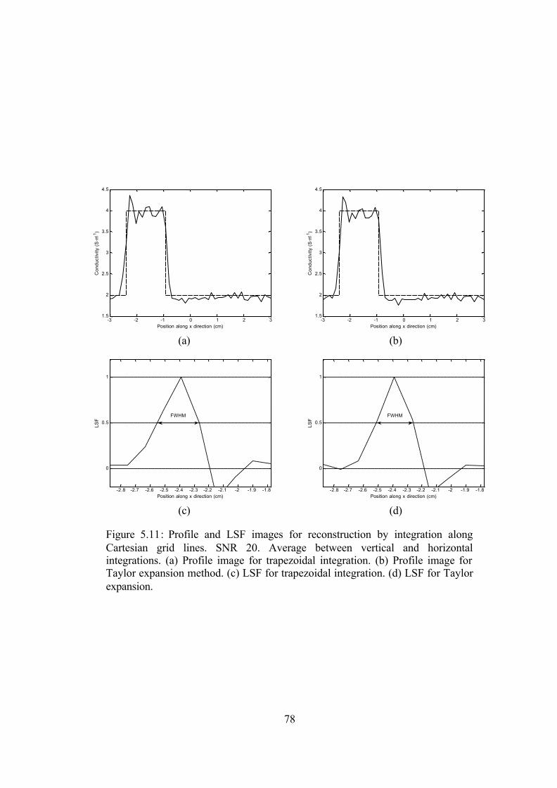
78

-3 -2 -1 0 1 2 31.5

2

2.5

3

3.5

4

4.5

Position along x direction (cm)

Con

duct

ivity

(S

·m-1

)

-3 -2 -1 0 1 2 31.5

2

2.5

3

3.5

4

4.5

Position along x direction (cm)

Con

duct

ivity

(S

·m-1

)

(a) (b)

-2.8 -2.7 -2.6 -2.5 -2.4 -2.3 -2.2 -2.1 -2 -1.9 -1.8

0

0.5

1

Position along x direction (cm)

LSF

FWHM

-2.8 -2.7 -2.6 -2.5 -2.4 -2.3 -2.2 -2.1 -2 -1.9 -1.8

0

0.5

1

Position along x direction (cm)

LSF

FWHM

(c) (d)

Figure 5.11: Profile and LSF images for reconstruction by integration along Cartesian grid lines. SNR 20. Average between vertical and horizontal integrations. (a) Profile image for trapezoidal integration. (b) Profile image for Taylor expansion method. (c) LSF for trapezoidal integration. (d) LSF for Taylor expansion.

79

5.6.3 Reconstruction by Solution of a Linear Equation System

In this section, the reconstructed images of the conductivity models using the

finite difference set of equations algorithm, described in Section 3.4 are given.

The effects of different noise levels are considered.

By setting one single point with the true resistivity (e.g. the left-upper corner), as

explained previously, the absolute conductivity image can be obtained. The

reconstructed conductivity image for the noise-free case can be seen in Figure

5.12(a). The finite difference method provokes artifacts in grid shape, since one

pixel is related with the four around. Besides, the contours of the objects are very

well defined.

For the noise cases, the performance of the algorithm have been tested with SNR

equal to 60, 30, 20, 10 and 5. In Figure 5.12, the resulting conductivity images

can be seen, from (b) to (f), respectively. The Table 5.8 shows the errors in the

reconstruction. It can be seen that the algorithm is very robust against noise.

Even in the case of SNR equal to 5, the objects can be inferred, although the

committed errors are important.

Table 5.8: Errors in reconstruction by solution of a linear equation system

Reconstructed Conductivity

Circle ( Circσε ) (%)

Rectangle ( Rectσε ) (%)

Background ( Bkcgσε ) (%)

Total error (%)

Noise-free 10.69 13.84 4.32 8.67 SNR 60 11.12 13.85 5.20 9.07 SNR 30 13.68 13.57 7.11 10.38 SNR 20 13.25 13.41 8.15 10.61 SNR 10 26.73 20.74 20.14 21.85 SNR 5 69.45 37.65 52.88 53.15

Therefore, this algorithm needs to specify the resistivity at a single point in order

to reconstruct true conductivity distribution. Moreover, it is very robust against

noise, being able to reconstruct with SNR equal to 5.

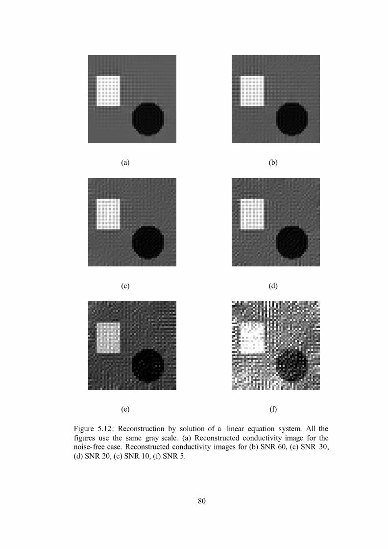
80

(a) (b)

(c) (d)

(e) (f)

Figure 5.12: Reconstruction by solution of a linear equation system. All the figures use the same gray scale. (a) Reconstructed conductivity image for the noise-free case. Reconstructed conductivity images for (b) SNR 60, (c) SNR 30, (d) SNR 20, (e) SNR 10, (f) SNR 5.

81

5.6.4 Reconstruction with Equipotential – Projection Algorithm

This section contains the results and discussion of the reconstructed conductivity

images, using the method described in Section 3.5. The effects of different noise

levels are studied. The true conductivity distribution can be reconstructed if at

least at one point it is known. The result can be seen in Figure 5.13(a).

The equipotential paths are calculated by starting ten equipotential lines per pixel

from the left edge of the phantom, in the same way as previously explained in

Section 5.6.1. Similar problems to the reconstruction by integration along

equipotential lines method have been observed.

In the noise-free reconstructed conductivity image, Figure 5.13 (b), the darkest

pixels in the upper and lower regions are set to zero conductivity, due to the lack

of equipotential lines crossing those pixels. In these regions, the potential cannot

be set, but a zero value is assigned, instead. By imposing this, the calculated

gradient of potential at the boundaries of these regions shows a big discontinuity

and, therefore, the reconstructed conductivity values have large errors. These

unset regions are not taken into consideration for error calculations, given in

Table 5.9. However, as said before, the pixels just in the border with those

regions make the error values increase very significantly. For example, just under

the circle, these transition effects can be seen. As a result, the background error

becomes more important than in previous reconstruction algorithms.

As the simulated noise level in the current density increases, the calculated

equipotential lines are heavily affected and many must be discarded. Therefore,

many pixels will not be crossed by any equipotential line and their values will

remain unknown. Another consequence is that some pixels can be isolated

between regions of unknown value and the integration can produce huge

numbers, provoking very large errors. This effect is very noticeable for the case

of SNR equal to 20.

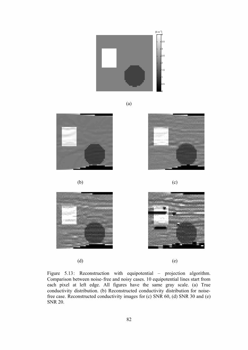
82

[S·m-1]

0

0.5

1

1.5

2

2.5

3

3.5

4

(a)

(b) (c)

(d) (e)

Figure 5.13: Reconstruction with equipotential – projection algorithm. Comparison between noise-free and noisy cases. 10 equipotential lines start from each pixel at left edge. All figures have the same gray scale. (a) True conductivity distribution. (b) Reconstructed conductivity distribution for noise-free case. Reconstructed conductivity images for (c) SNR 60, (d) SNR 30 and (e) SNR 20.

83

Table 5.9: Errors in reconstruction with equipotential – projection algorithm

Reconstructed Conductivity

Circle ( Circσε ) (%)

Rectangle ( Rectσε ) (%)

Background ( Bkcgσε ) (%)

Total error (%)

Noise-free 9.13 7.16 18.83 16.05 SNR 60 13.94 14.39 19.95 18.34 SNR 30 23.37 17.73 23.49 21.92 SNR 20 18.20 31.92 2 x 1015 2 x 1015

Therefore, this algorithm is also very sensitive to noise. The absence of

equipotential lines provokes very important errors in the pixels nearby. As

before, this method needs to know the resistivity for at least one point in order to

reconstruct true conductivity images.

5.6.5 Reconstruction using J-substitution Algorithm

In this section, the conductivity images produced by this last current density

based algorithm, described in Section 3.6, are given. The effects of different

noise levels and electrode sizes are studied. The corresponding errors are given

in Table 5.10.

This iterative reconstruction algorithm begins setting an initial uniform resistivity

distribution 0 1ρ = to the whole image. Two orthogonal current profiles have

been used, as defined previously in Figure 5.1. In each iteration, the forward

problem defined in (3.45) is solved for one injection profile by cell-centered

finite difference method. Thus, the solution of the linear system (2.39) yields a

conductivity distribution, which is used as initial guess for the next iteration,

where the other injection profile is utilized.

As it was stated previously in Section 5.4, two different stopping criteria can be

used to terminate the iterations: if the difference in resistivity between two

successive iterations is below a given threshold, or the error with respect to the

true distribution, which is known in these simulation cases, is minimum.

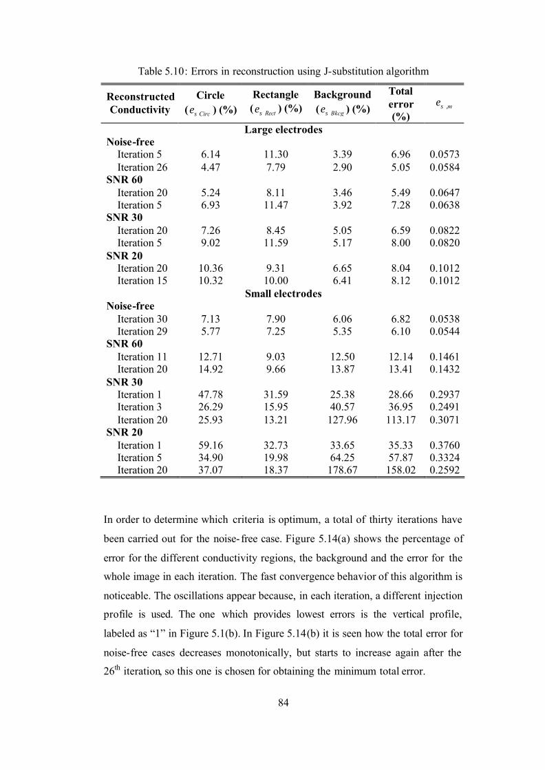
84

Table 5.10: Errors in reconstruction using J-substitution algorithm

Reconstructed Conductivity

Circle ( Circσε ) (%)

Rectangle ( Rectσε ) (%)

Background ( Bkcgσε ) (%)

Total error (%)

,mσε

Large electrodes Noise-free Iteration 5 6.14 11.30 3.39 6.96 0.0573 Iteration 26 4.47 7.79 2.90 5.05 0.0584 SNR 60 Iteration 20 5.24 8.11 3.46 5.49 0.0647 Iteration 5 6.93 11.47 3.92 7.28 0.0638 SNR 30 Iteration 20 7.26 8.45 5.05 6.59 0.0822 Iteration 5 9.02 11.59 5.17 8.00 0.0820 SNR 20 Iteration 20 10.36 9.31 6.65 8.04 0.1012 Iteration 15 10.32 10.00 6.41 8.12 0.1012

Small electrodes Noise-free Iteration 30 7.13 7.90 6.06 6.82 0.0538 Iteration 29 5.77 7.25 5.35 6.10 0.0544 SNR 60 Iteration 11 12.71 9.03 12.50 12.14 0.1461 Iteration 20 14.92 9.66 13.87 13.41 0.1432 SNR 30 Iteration 1 47.78 31.59 25.38 28.66 0.2937 Iteration 3 26.29 15.95 40.57 36.95 0.2491 Iteration 20 25.93 13.21 127.96 113.17 0.3071 SNR 20 Iteration 1 59.16 32.73 33.65 35.33 0.3760 Iteration 5 34.90 19.98 64.25 57.87 0.3324 Iteration 20 37.07 18.37 178.67 158.02 0.2592

In order to determine which criteria is optimum, a total of thirty iterations have

been carried out for the noise-free case. Figure 5.14(a) shows the percentage of

error for the different conductivity regions, the background and the error for the

whole image in each iteration. The fast convergence behavior of this algorithm is

noticeable. The oscillations appear because, in each iteration, a different injection

profile is used. The one which provides lowest errors is the vertical profile,

labeled as “1” in Figure 5.1(b). In Figure 5.14(b) it is seen how the total error for

noise-free cases decreases monotonically, but starts to increase again after the

26th iteration, so this one is chosen for obtaining the minimum total error.

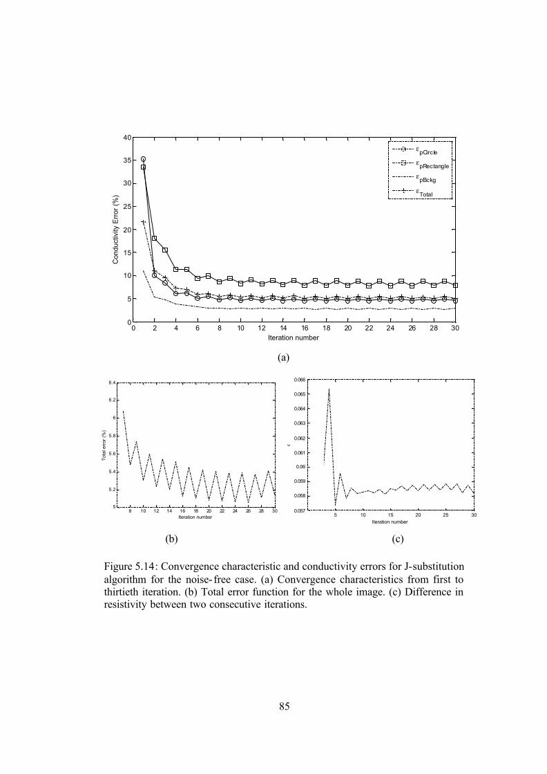
85

0 2 4 6 8 10 12 14 16 18 20 22 24 26 28 300

5

10

15

20

25

30

35

40

Iteration number

Con

duct

ivity

Err

or (

%)

εpCircle

εpRectangle

εpBckg

εTotal

(a)

8 10 12 14 16 18 20 22 24 26 28 305

5.2

5.4

5.6

5.8

6

6.2

6.4

Iteration number

Tota

l err

or (

%)

5 10 15 20 25 300.057

0.058

0.059

0.06

0.061

0.062

0.063

0.064

0.065

0.066

Iteration number

ε

(b) (c)

Figure 5.14: Convergence characteristic and conductivity errors for J-substitution algorithm for the noise-free case. (a) Convergence characteristics from first to thirtieth iteration. (b) Total error function for the whole image. (c) Difference in resistivity between two consecutive iterations.

86

Besides, the difference in conductivity between two consecutive iterations is

shown in Figure 5.14(c), There is a minimum for the 5th iteration, so this

threshold is taken to satisfy the first criterion. Only the conductivity image for

the 26th iteration in noise-free case is shown in Figure 5.15(b), because the

difference is practically imperceptible.

Moreover, different levels of noise in the simulated current density data are

added, and their effects are studied. The resulting images are also displayed in

Figure 5.15. The convergence curve, defined as the total error of the

reconstructed image in each iteration, for all noise levels is shown in Figure

5.19(a). It is noticeable that the algorithm always converges, and reconstructs

with only 8% of error when SNR is 20.

Since Kwon et al [20] use small electrodes in their study, this case is now

considered. The electrode sizes are chosen as one third of the phantom edge

width. The total conductivity distribution is shown in Figure 5.16, while the

reconstructed images are given in Figure 5.18. The noise-free case presents a

similar figure, but, when the no ise increases and becomes considerable, the

algorithm diverges, as shown in the convergence curve in Figure 5.19(b). In

order to find the best result, there is a compromise between the total error, mainly

due to the divergence of the background, and the errors corresponding to the

objects which are wanted to be reconstructed. This can be seen in Figure 5.17.

The reconstruction errors are given in Table 5.10. As it can be seen, in some

cases, the minimum total error may be preferred, while in other cases, a

minimum error in reconstructing a particular conductivity region may be a

priority. The main contributor to this large error in the background seems to be

the corners, which become reconstructed badly and with higher values as the

number of iterations increases. This is because the electrodes are small and

centered. The current is not spread uniformly, and very low amount of current

reaches the corners.

87

(a)

(b) (c)

(d) (e)

Figure 5.15: Reconstruction for J-substitution algorithm. Large electrodes. All figures have the same gray scale. (a) True distribution. (b) Noise-free case. Iteration 26. (c) SNR 60. Iteration 20. (d) SNR 30. Iteration 20. (f) SNR 20. Iteration 20.

88

(a) (b)

Figure 5.16: Total current density distribution for small electrodes, for injection patterns 1 (a) and 2 (b)

0 2 4 6 8 10 12 14 16 18 200

50

100

150

Iteration number

Con

duct

ivity

Err

or (

%)

εpCircle

εpRectang le

εpBckg

εTo tal

0 2 4 6 8 10 12 14 16 18 200

20

40

60

80

100

120

140

160

180

Iteration number

Con

duct

ivity

Err

or (

%)

εpCir cle

εpRectangle

εpBc kg

εTota l

(a) (b)

Figure 5.17: Convergence characteristic of J-substitution algorithm for small electrodes. (a) SNR equal to 30. (b) SNR equal to 20.

89

(a)

(b) (c)

(d) (e)

Figure 5.18: Reconstruction for J-substitution algorithm. Small electrodes. All figures have the same gray scale. (a) True distribution. (b) Noise-free case. Iteration 29. (c) SNR 60. Iteration 20. (d) SNR 30. Iteration 3. (f) SNR 20. Iteration 5.

90

0 2 4 6 8 10 12 14 16 18 204

6

8

10

12

14

16

18

20

22

24

Iteration number

Con

duct

ivity

Err

or (

%)

Noise-freeSNR60

SNR30

SNR20

(a)

0 2 4 6 8 10 12 14 16 18 200

20

40

60

80

100

120

140

160

Iteration number

Con

duct

ivity

Err

or (

%)

Noise-freeSNR60

SNR30

SNR20

(b)

Figure 5.19: Convergence characteristic of J-substitution algorithm with different noise levels, with (a) large electrodes; (b) small electrodes.

91

Therefore, this iterative algorithm yields very low errors when the electrodes

cover the whole sides, as the previous algorithms. An initial resistivity

distribution is needed, but a reasonable guess is enough to make it converge.

Another requirement is the measurement of the voltage between the electrodes in

order to get a true conductivity image. One disadvantage is that, since it is

iterative, it needs a lot of computation time and resources in order to solve the

forward problem for each iteration. This depends on the level of noise and size of

the image. For example, in an AMD64 3000+, 2 GB of RAM, Matlab R2006b on

Windows XP x64 SP1, the 20 iterations for the noise-free case and large

electrodes could take around three hours.

5.7 Simulation Results for Magnetic Flux Density Based

Algorithms

In this section, the reconstructed conductivity images produced by the Harmonic

Bz algorithm, described in chapter 4, are given and discussed. This algorithm has

been tested for the simulated phantom described in 5.2.1, under different noise

levels.

This iterative reconstruction algorithm begins assuming an initial uniform

conductivity distribution 0 1σ = for the whole image. Two orthogonal current

profiles have been used, as defined previously in Figure 5.1. In each iteration, the

forward problem defined in (4.11) is solved for each injection profile by cell-

centered finite difference method. Then, a new conductivity distribution is

calculated using (4.6), (4.9) and (4.10), and fed into the next iteration.

Figure 5.20 shows the reconstructed images for different noise levels after six

iterations, where the tolerance 0.05ε = has been used as stopping criterion. In

Table 5.11, the corresponding errors for each case are given. It is observed that

the algorithm converges quickly and the errors remain low, due to the iterative

characteristic of this method. Another observation is that even when the error

grows as the SNR decreases, the appearance of the images remains quite

acceptable. The main drawback of this method is the large computation time for

92

each iteration. For example, for the same equipment as described above, each

iteration could cost around 40 minutes.

Table 5.11: Errors in reconstruction using Harmonic Bz algorithm

Reconstructed Conductivity

Circle ( Circσε ) (%)

Rectangle ( Rectσε ) (%)

Background ( Bkcgσε ) (%)

Total error (%)

,mσε

Large electrodes Noise-free Iteration 6 8.51 4.50 5.08 5.37 0.049 SNR 60 Iteration 6 8.72 12.41 10.96 12.09 0.049 SNR 30 Iteration 6 12.84 13.61 12.97 14.03 0.050 SNR 20 Iteration 6 16.62 17.23 16.27 17.11 0.050

93

2 4 60

5

10

15

20

25

30

35

40

45

50

Iteration number

Con

duct

ivity

Err

or (

%)

εpCircle

εpRectangle

εpBckg

εTotal

(a) (b)

(c) (d)

(e) (f)

Figure 5.20: Reconstruction for Harmonic Bz algorithm. Large electrodes. All figures have the same gray scale. (a) True distribution. Reconstructed images are given at 6th iteration. (b) Convergence characteristic for the noise-free case. (c) Noise-free case. (d) SNR 60. (e) SNR 30. (f) SNR 20.

94

5.8 Partial FOV/ROI reconstruction

These algorithms can also reconstruct a region of interest (ROI) within the

image, instead of obtaining the full field of view (FOV). This feature can be

applied in some practical applications, where optimum injection patterns for

specific conductivity regions are used. Thus, a full FOV can be better

reconstructed by combining different optimized ROI.

As an example, two different ROI’s, defined in Figure 5.21(a), have been

reconstructed using the equipotential-projection algorithm, with a single

measurement point, for the noise-free case. As in the previous Section 5.6.4, the

lack of equipotential lines provides unknown conductivity values, which are

shown as the darkest areas in the reconstructed images in Figure 5.21. The

borders of these areas, due to the gradient operator intrinsic to this algorithm,

produce conductivity values with high error, which, consequently, raise heavily

the error of the conductivity region at which they belong to.

Table 5.12: Errors in reconstructing different ROI

Reconstructed ROI

Circle ( Circσε ) (%)

Rectangle ( Rectσε ) (%)

Background ( Bkcgσε ) (%)

Total error (%)

ROI 1 N. A. 8.44 11.85 9.42 ROI 2 17.55 N. A. 23.15 24.56

95

ROI 2

ROI 1

(a)

(b) (c)

-2.76 -0.24-0.72

1.80

-0.84 2.76-3

0.60

(d) (e)

Figure 5.21: Reconstruction of two different ROI’s with equipotential-projection algorithm. All figures have the same gray scale. (a) True distribution with the definition of ROI1 and ROI2. Reconstructed images for (b) ROI1 and (c) ROI2, with 10 equipotential lines starting from each pixel at left edge. Equipotential lines for (d) ROI1 and (e) ROI2. In order to distinguish them easily, in (d), only 4 equipotential lines have been started per each left-side pixel, while 3 equipotential lines have been used in (e).

96

5.9 Comparison between reconstruction algorithms

In this section, the previous reconstruction algorithms are compared under the

same conditions for simulated and experimental data. The resulting images are

taken as the direct output of the reconstruction algorithms, without applying any

image processing.

5.9.1 Simulated data

The simulated data corresponds to the numerical phantom previously defined in

Section 5.2.1 and shown in Figure 5.22. The reconstructed algorithms are

compared for the noise-free case and different noise levels. Errors committed in

the reconstruction and blurring effects are studied and quantified.

Figure 5.22: True conductivity distribution. Exact locations of the different conductivity regions are shown. The dashed line gives the definition for the profile image.

5.9.1.1 Noise-free case

For noise-free simulated data, the reconstruction algorithms are evaluated under

the following set of conditions : large electrodes, ten equipotential lines per pixel,

trapezoidal integration method and averaging between vertical and horizontal

integration, if applicable. The reconstructed conductivity images for each

algorithm are presented in Figure 5.23. The committed errors are given in Table

5.13. In Figure 5.24, the horizontal profiles for a line crossing an edge of the

97

rectangle, as defined in Figure 5.22, are shown. Besides, in Figure 5.25, the Line

Spread Functions for the conductivity profiles can be observed. Finally, the

calculated LSF widths at FWHM are given in Table 5.14.

Considering only the committed errors, it can be seen that the methods which

give the lowest overall one are the iterative algorithms: J-substitution and

Harmonic Bz algorithms. This kind of methods corrects themselves iteration by

iteration, and if they converge, as in these cases, the provided images are quite

accurate. Moreover, the error committed at reconstructing the different

conductivity regions is generally lower than in the non- iterative ones. Notice that

the condition of large electrodes, in the J-substitution algorithm, provides lower

error than small electrodes, due to the decrease of current, and therefore

information, near the phantom edges. The main disadvantage of the iterative

methods is their large computation time, usually some hours. The direct methods,

however, are practically instantaneous. This correction effect could be used to

improve the quality of the reconstruction by feeding one of these iterative

methods with the solution of a direct one, as initial conductivity distribution.

Table 5.13: Comparison for the noise-free case

Reconstruction Algorithms

Circle ( Circσε ) (%)

Rectangle ( Rectσε ) (%)

Background ( Bkcgσε ) (%)

Total error (%)

Solution of Linear Equation System

10.69 13.84 4.32 8.67

Integration Along Cartesian Grid Lines

13.37 8.54 4.35 6.44

Integration Along Equipotential Lines

17.69 12.15 9.74 11.36

Equipotential – Projection

9.13 7.16 18.83 16.05

J-substitution (large electrodes)

4.47 7.79 2.90 5.05

J-substitution (small electrodes) 5.77 7.25 5.35 6.10

Harmonic Bz 8.51 4.50 5.08 5.37

98

(a) (b)

(c) (d)

(e) (f)

Figure 5.23: Comparison for the noise-free case. All figures have the same gray scale. (a) Reconstruction by solution of linear equation system by finite differences. (b) Trapezoidal integration along cartesian grid lines. Average of vertical and horizontal integration. (c) Trapezoidal integration along equipotential lines. 10 equipotential lines per pixel. (d) Reconstruction with equipotential – projection algorithm. 10 equipotential lines per pixel. (e) J-substitution algorithm with large electrodes. Iteration 26. (f) Bz algorithm. Iteration 6.

99

-3 -2 -1 0 1 2 31.5

2

2.5

3

3.5

4

4.5

Position along x direction (cm)

Con

duct

ivity

(S

·m-1

)

-3 -2 -1 0 1 2 31.5

2

2.5

3

3.5

4

4.5

Position along x direction (cm)

Con

duct

ivity

(S

·m-1

)

(a) (b)

-3 -2 -1 0 1 2 31.5

2

2.5

3

3.5

4

4.5

Position along x direction (cm)

Con

duct

ivity

(S

·m-1

)

-3 -2 -1 0 1 2 31.5

2

2.5

3

3.5

4

4.5

Position along x direction (cm)

Con

duct

ivity

(S

·m-1

)

(c) (d)

-3 -2 -1 0 1 2 31.5

2

2.5

3

3.5

4

4.5

Position along x direction (cm)

Con

duct

ivity

(S

·m-1

)

-3 -2 -1 0 1 2 31.5

2

2.5

3

3.5

4

4.5

Position along x direction (cm)

Con

duct

ivity

(S

·m-1

)

(e) (f)

Figure 5.24: Profile images for the noise-free case. (a) Reconstruction by solution of linear equation system by finite differences. (b) Trapezoidal integration along cartesian grid lines. Average of vertical and horizontal integration. (c) Trapezoidal integration along equipotential lines. 10 equipotential lines per pixel. (d) Reconstruction with equipotential – projection algorithm. 10 equipotential lines per pixel. (e) J-substitution algorithm with large electrodes. Iteration 26. (f) Bz algorithm. Iteration 6.

100

-2.8 -2.7 -2.6 -2.5 -2.4 -2.3 -2.2 -2.1 -2 -1.9 -1.8

0

0.5

1

Position along x direction (cm)

LSF

FWHM

-2.8 -2.7 -2.6 -2.5 -2.4 -2.3 -2.2 -2.1 -2 -1.9 -1.8

0

0.5

1

Position along x direction (cm)

LSF

FWHM

(a) (b)

-2.8 -2.7 -2.6 -2.5 -2.4 -2.3 -2.2 -2.1 -2 -1.9 -1.8

0

0.5

1

Position along x direction (cm)

LSF

FWHM

-2.8 -2.7 -2.6 -2.5 -2.4 -2.3 -2.2 -2.1 -2 -1.9 -1.8

0

0.5

1

Position along x direction (cm)

LSF

FWHM

(c) (d)

-2.8 -2.7 -2.6 -2.5 -2.4 -2.3 -2.2 -2.1 -2 -1.9 -1.8

0

0.5

1

Position along x direction (cm)

LSF

FWHM

-2.8 -2.7 -2.6 -2.5 -2.4 -2.3 -2.2 -2.1 -2 -1.9 -1.8

0

0.5

1

Position along x direction (cm)

LSF

FWHM

(e) (f)

Figure 5.25: LSF images for the noise-free case. (a) Reconstruction by solution of linear equation system by finite differences. (b) Trapezoidal integration along cartesian grid lines. Average of vertical and horizontal integration. (c) Trapezoidal integration along equipotential lines. 10 equipotential lines per pixel. (d) Reconstruction with equipotential – projection algorithm. 10 equipotential lines per pixel. (e) J-substitution algorithm with large electrodes. Iteration 26. (f) Bz algorithm. Iteration 6.

101

On the other hand, if the lowest blurring effect is considered, the reconstruction

by solving a linear equation system provides the lowest LSF width and therefore,

the sharpest image. The reconstruction with equipotential – projection algorithm

gives the following sharpest conductivity image. The iterative algorithms,

however, provide intermediate LSF widths. Finally, the two integration

algorithms present the highest blurring effects. The main reason for this is the

error accumulation that this technique suffers from, besides the integration

method used: trapezoidal, instead of Taylor expansion.

Table 5.14: FWHM of LSF. Comparison for the noise-free case

Reconstruction Algorithms FWHM (cm) Solution of Linear Equation System 0.213

Integration Along Cartesian Grid Lines 0.309

Integration Along Equipotential Lines 0.297

Equipotential – Projection 0.246

J-substitution (large electrodes) 0.282

Harmonic Bz 0.278

Comparing now the method of integration along equipotential lines and along

cartesian grid lines, it is seen how the latter gives less error. In part, it is due to

the average performed between vertical and horizontal integration, but also since

the calculated equipotential paths are an approximation to the real ones. The

current vectors are assumed to be constant within a pixel, but if it is too big, this

assumption cannot be valid. This may happen where the current lines

accumulate, for example, at the interface between two regions with different

conductivity. It also occurs where the current flow is very little, like at the

corners, especially in the case where the electrodes are small compared with the

size of the phantom. In the images, the bias effect of the integration along the

equipotential paths can be seen in Figure 5.23(c), while in (b) this effect is

counteracted, due to averaging.

102

The reconstruction by solving a linear equation system provides an intermediate

solution. The error is not the largest, or the smallest, and the reconstructed image

is the least blurred one. One disadvantage is that the image suffers from a grid

effect due to the discretization of the finite difference method. This especially

makes the rectangle be slightly more erroneous than in the rest of cases and a

worse appearance.

The method which provides the largest overall error is the equipotential –

projection algorithm, although it is one of the algorithms with sharpest and best

defined object contours, especially in the circular object. The reason for the large

error is that the regions which are not passed by any equipotential lines remain

with unknown values, representing a big discontinuity. When the gradient of the

potential is calculated during an intermediate step of the algorithm, these

discontinuities provoke important errors in the pixels surrounding these unknown

areas. In this case, they are located in the background, so the error at

reconstructing the background becomes quite important, even considering that

the dark pixels are actually not considered in the error calculation.

5.9.1.2 Noisy cases

In this section, the reconstruction algorithms are compared for a noise level of

SNR equal 20. At this noise level, all algorithms can reconstruct images with

tolerable errors. The same conditions as in the previous section hold for all the

algorithms in order to evaluate them: large electrodes, ten equipotential lines per

pixel, trapezoidal integration method and averaging between vertical and

horizontal integration, if applicable. The reconstructed conductivity images for

each algorithm are presented in Figure 5.26. The committed errors are given in

Table 5.15. In Figure 5.27, the horizontal profiles for a line crossing an edge of

the rectangle, as previously defined in Figure 5.22, are shown. Moreover, in

Figure 5.28, the Line Spread Functions for the conductivity profiles can be

observed. Finally, the calculated LSF widths at FWHM are given in Table 5.16.

103

Table 5.15: Comparison for noisy cases. SNR equal to 20

Reconstruction Algorithms

Circle ( Circσε ) (%)

Rectangle ( Rectσε ) (%)

Background ( Bkcgσε ) (%)

Total error (%)

Solution of Linear Equation System 13.25 13.41 8.15 10.61

Integration Along Cartesian Grid Lines

15.61 11.95 7.53 9.74

Integration Along Equipotential Lines

25.23 25.65 20.12 23.30

Equipotential – Projection 18.20 31.92 2 x 1015 2 x 1015

J-substitution (large electrodes) 10.36 9.31 6.65 8.04

Harmonic Bz 16.62 17.23 16.27 17.11

Considering only the overall error, the reconstruction algorithm which gives the

lowest error is the J-substitution algorithm at its 20th iteration, as in the noise-free

case. Moreover, the error committed at reconstructing the different conductivity

regions are lower than in the rest of algorithms. The resulting image has very

good quality, apart from an important salt-and-pepper noise, and being the one

with most blurred edges. However, it is necessary to notice that this method can

diverge when the noise is too high. Therefore, a careful study of its convergence

must be carried out, in order to decide which iteration provides the minimum

desired error: in total, in a particular area, a balance, etc. If the size of the

electrodes is reduced, this algorithm becomes more sensitive to noise and can

diverge easier (see Section 5.6.5), since the current flow is not spread uniformly

throughout the whole field of view. The other iterative method, the Harmonic Bz

algorithm, suffers from larger error, even though the image could be considered

as the one with the best appearance.

If the blurring effect is considered as a criterion, the reconstruction by solving a

linear equation system provides the lowest LSF width at FWHM, and the

reconstruction by integration along Cartesian grid lines provides the largest, as in

104

the noise-free case. The iterative algorithms produce intermediate blurred

images. Although the image reconstructed by reconstruction along equipotential

lines is quite blurred, the LSF width calculated at the defined profile row gives,

by chance, a very good figure.

Table 5.16: FWHM of LSF. Comparison for noisy cases. SNR equal to 20

Reconstruction Algorithms FWHM (cm) Solution of Linear Equation System 0.192

Integration Along Cartesian Grid Lines 0.287

Integration Along Equipotential Lines 0.200

Equipotential – Projection 0.267

J-substitution (large electrodes) 0.319

Harmonic Bz 0.283

The integration along Cartesian grid lines and solution of linear system come to

similar overall errors, although the reconstructed image of the latter has a better

looking, since, in the former one, the integration technique spreads the errors

along the direction of integration.

The method which provides largest error is the equipotential – projection

algorithm. As the noise increases, less equipotential lines are valid, since the

directions of current vectors become more random, and the calculated

equipotential lines, orthogonal to these vectors, tend to cross each other. Those

invalid equipotential paths are removed, as explained before. Thus, more

unknown areas appear and, due to the gradient operator involved in the

algorithm, the calculation of the conductivity at the surrounding pixels provide

erroneous values, sometimes very huge, as shown in Table 5.15.

105

(a) (b)

(c) (d)

(e) (f)

Figure 5.26: Comparison for SNR equal to 20. All figures have the same gray scale. (a) Reconstruction by solution of linear equation system. (b) Trapezoidal integration along cartesian grid lines. Average of vertical and horizontal integration. (c) Trapezoidal integration along equipotential lines. 10 equipotential lines per pixel. (d) Reconstruction with equipotential – projection algorithm. 10 equipotential lines per pixel. (e) J-substitution algorithm with large electrodes. Iteration 20. (f) Bz algorithm. Iteration 6.

106

-3 -2 -1 0 1 2 31.5

2

2.5

3

3.5

4

4.5

Position along x direction (cm)

Con

duct

ivity

(S

·m-1

)

-3 -2 -1 0 1 2 31.5

2

2.5

3

3.5

4

4.5

Position along x direction (cm)

Con

duct

ivity

(S

·m-1

)

(a) (b)

-3 -2 -1 0 1 2 30.5

1

1.5

2

2.5

3

3.5

4

4.5

Position along x direction (cm)

Con

duct

ivity

(S

·m-1

)

-3 -2 -1 0 1 2 31.5

2

2.5

3

3.5

4

4.5

Position along x direction (cm)

Con

duct

ivity

(S

·m-1

)

(c) (d)

-3 -2 -1 0 1 2 31.5

2

2.5

3

3.5

4

4.5

Position along x direction (cm)

Con

duct

ivity

(S

·m-1

)

-3 -2 -1 0 1 2 31.5

2

2.5

3

3.5

4

4.5

Position along x direction (cm)

Con

duct

ivity

(S

·m-1

)

(e) (f)

Figure 5.27: Profile images for SNR equal to 20. (a) Reconstruction by solution of linear equation system. (b) Trapezoidal integration along cartesian grid lines. Average of vertical and horizontal integration. (c) Trapezoidal integration along equipotential lines. 10 equipotential lines per pixel. (d) Reconstruction with equipotential – projection algorithm. 10 equipotential lines per pixel. (e) J-substitution algorithm with large electrodes. Iteration 20. (f) Bz algorithm. Iteration 6.

107

-2.8 -2.7 -2.6 -2.5 -2.4 -2.3 -2.2 -2.1 -2 -1.9 -1.8

0

0.5

1

Position along x direction (cm)

LSF

FWHM

-2.8 -2.7 -2.6 -2.5 -2.4 -2.3 -2.2 -2.1 -2 -1.9 -1.8

0

0.5

1

Position along x direction (cm)

LSF

FWHM

(a) (b)

-2.8 -2.7 -2.6 -2.5 -2.4 -2.3 -2.2 -2.1 -2 -1.9 -1.8

0

0.5

1

Position along x direction (cm)

LSF

FWHM

-2.8 -2.7 -2.6 -2.5 -2.4 -2.3 -2.2 -2.1 -2 -1.9 -1.8

0

0.5

1

Position along x direction (cm)

LSF

FWHM

(c) (d)

-2.8 -2.7 -2.6 -2.5 -2.4 -2.3 -2.2 -2.1 -2 -1.9 -1.8

0

0.5

1

Position along x direction (cm)

LSF

FWHM

-2.8 -2.7 -2.6 -2.5 -2.4 -2.3 -2.2 -2.1 -2 -1.9 -1.8

0

0.5

1

Position along x direction (cm)

LSF

FWHM

(e) (f)

Figure 5.28: LSF images for SNR equal to 20. (a) Reconstruction by solution of linear equation system. (b) Trapezoidal integration along cartesian grid lines. Average of vertical and horizontal integration. (c) Trapezoidal integration along equipotential lines. 10 equipotential lines per pixel. (d) Reconstruction with equipotential – projection algorithm. 10 equipotentia l lines per pixel. (e) J-substitution algorithm with large electrodes. Iteration 20. (f) Bz algorithm. Iteration 6.

108

5.9.2 Experimental data

In this section, the reconstruction algorithms are fed with the real data measured

by [24] and [2], using the experimental phantom defined in 5.2.2 into the 0.15

Tesla METU-EE MRI system. The reconstructed images can be seen in Figure

5.30. The errors committed in the reconstruction are given in Table 5.17.

Only measured current density distribution corresponding to the horizontal

injection pattern is available [24]. This is shown in Figure 5.29(a) and (b). A

great amount of noise present in the data is noticeable. Since the object is

symmetric, the current density distribution for the vertical injection pattern is

obtained by transposition of the measured data corresponding to the horizontal

injection case.

The calculation of the equipotential lines using the procedure described in 3.2.1.1

provides extremely few valid equipotential lines. For example, for the vertical

injection case, the equipotential lines are started from the left edge, and they

travel orthogonal to the current streams at every pixel, until they reach the right

edge. But, the amount of current decreases dramatically at the right and left sides,

since the electrodes are very small and the conductor has a large conductivity.

Due to this reason, these regions are very sensitive to noise. Consequently, the

current vectors at the sides are very random and very few equipotential lines can

arrive to the conductor at the center and reach the right edge of the image. This

situation can be observed in Figure 5.31. As a result, under such noisy

conditions, conductivity images can not be reconstructed well by equipotential

line based algorithms.

109

(a)

-0.5

-0.4

-0.3

-0.2

-0.1

0

0.1

0.2

0.3

0.4

0

0.05

0.1

0.15

0.2

0.25

0.3

0.35

0.4

(b) (c)

-3 3-3

3

-3 3-3

3

(d) (e)

Figure 5.29: Measured current density distributions for the experimental data. (a) True conductivity distribution. (b) yJ for the horizontal injection case. (c) xJ for the horizontal injection case. (d) Current density distribution for the horizontal injection pattern. (e) Current density distribution for the vertical injection pattern.

110

(a) (b)

(c) (d)

0 2 4 6 8 10 12 14 16 18 200

50

100

150

200

250

300

350

400

450

500

Iteration number

Con

duct

ivity

Err

or (

%)

εpSquare

εpBckg

εTotal

(e) (f)

Figure 5.30: Comparison for experimental data. All figures have the same gray scale. (a) Reconstruction by solution of linear equation system. (b) Reconstruction by integration along Cartesian grid lines, averaging between vertical and horizontal integration. Reconstruction conductivity with J-substitution algorithm at iteration 1 (c) and iteration 20 (d). (e) Convergence characteristic of J-substitution algorithm. (f) Bz algorithm. Iteration 6.

111

Table 5.17: Comparison for experimental data

Reconstruction Algorithms

Rectangle ( Rectσε ) (%)

Background ( Bkcgσε ) (%)

Total error (%)

Solution of Linear Equation System

32.53 209.24 93.94

Integration Along Cartesian Grid Lines 107.07 2432 1059.2

J-substitution. Iteration 1 21.52 236.42 102.53

J-substitution. Iteration 20 39.56 468.57 202.68

Harmonic Bz. Iteration 6 47.06 310.84 121.24

-3 3-3

3

Figure 5.31: Equipotential lines for experimental data. 10 equipotential lines start from each pixel at the left side.

The rest of reconstruction algorithms can deal with this experimental data,

although the resulting images have very important errors, especially in the

background, due to the noise and small amount of current outside the conductor.

The J-substitution algorithm provides the smallest error for the rectangle, while

the reconstruction by solution of linear equation system gives the smallest total

error and best appearance. The rectangle, in this case, can be more clearly

inferred. The Harmonic Bz yields an intermediate solution. The reconstruction by

integration along Cartesian grid lines suffers from accumulation of error due to

the usage of integration, resulting in huge errors.

112

CHAPTER 6

CONCLUSIONS AND FUTURE WORK

6.1 Conclusions

In this study, a set of different reconstruction algorithms for MR-EIT, proposed

by several research groups have been implemented and their reconstruction

accuracies have been compared.

The MR-EIT reconstruction algorithms are classified into two groups: Type-I and

Type-II, depending on the input data they require to reconstruct conductivity

images. Type-I algorithms use current density distribution, calculated from

magnetic flux density data. Type-II algorithms, on the other hand, use directly the

magnetic flux density data. Both types use peripheral voltage measurements for

the reconstruction of the true conductivity values.

Five Type-I algorithms, previously proposed, are studied in this thesis. They are

the followings : reconstruction by integration along equipotential lines,

reconstruction by integration along Cartesian grid lines, reconstruction by

solution of a linear equation system by finite differences discretization,

reconstruction with equipotential – projection algorithm without potential

measurement, and J-substitution algorithm..

Currently, each study uses a different conductivity and noise model, injection

profiles, injected current, noise levels, etc. Therefore, in order to compare them

objectively, a set of conditions have been defined, so that all of them have been

implemented and tested under the same circumstances. Moreover, the output

113

images have been compared directly, without performing any image processing.

Reconstruction errors and spatial resolution have been quantified and compared.

In the noise-free case, the iterative algorithms: J-substitut ion and harmonic Bz

algorithm provide the lowest total error, 5.05% and 5.37%, respectively. For the

reconstruction along equipotential lines and equipotential – projection algorithm,

by using a single injection pattern, the equipotential lines can be traced

throughout the image, being orthogonal at every pixel to the current vector. But,

these equipotential lines may not cover the whole image, due to conductivity

changes inside the phantom. Those non-covered areas remain with unknown

conductivity, generating discontinuities and, indirectly, errors in the

reconstruction. Thus, the equipotential – projection algorithm gives the highest

total error, 16.05%, while the reconstruction along equipotential lines yields

11.36%. These figures may be reduced by obtaining the equipotential lines for

two orthogonal injection patterns and combining adequately the resulting images.

The integration along Cartesian grid lines and solution of a linear equation

system algorithms yield to similar intermediate errors: 6.44% and 8.67%,

respectively, although the latter one provides sharper contours. The methods

which provide less blur images are the solution of a linear equation system and

equipotential – projection algorithm. The methods which involve integrations

give the most blurred images. Finally, both iterative algorithms produce

intermediate blurring results.

In order to study the performance of the reconstruction algorithms in presence of

noise, different noisy current densities, corresponding to SNR noise levels equal

to 60, 30 and 20 are generated. When the SNR is smaller than 20, equipotential

lines cannot be traced, so the integration along equipotential lines and

equipotential – projection algorithms are very affected. In the latter one, few

pixels accumulate exaggerated values in the background, although the rest of

conductivity regions in the image have similar error values to the rest of

algorithms. As it was previously said, this effect may be reduced by using two

orthogonal injection patterns. The J-substitution algorithm, as in the noise-free

case, gives the lowest overall error, although it may diverge if the noise level is

below SNR equal 20, or if the electrode sizes become too small. The linear

114

equation system algorithm, however, is very robust against noise. It can

reconstruct with a noise level of SNR equal to 5 with a total error of 50%.

Moreover, it presents the sharpest reconstructed images, as in the noise-free case.

In the case of integration along Cartesian grid lines, although the overall errors

are not especially high, the resulting images become very blurred, since the

integration techniques tend to spread the errors along the direction of integration.

Finally, the harmonic Bz algorithm provides acceptable images, but with

intermediate reconstruction errors.

6.2 Future work

In this thesis, a set of different reconstruction algorithms have been implemented

and compared. Some of the possible further work can be:

• Validate the simulated results with more measured data.

• Define and set up a complete test bed, in order to be able to compare

rapidly and in an automatic way very different aspects of the incoming

and previously proposed algorithms: spatial resolution, different injection

profiles, size of electrodes, object placements, noise levels, etc.

• Apart from comparing the reconstructed images objectively, other

perceptual methods could be used, additionally.

115

REFERENCES

[1] D. C. Barber and B. H. Brown, “Applied Potential Tomography

(Review Article)”, J. Phys. E. Sci.Instrum, vol. 17, pp. 723 – 733, 1984.

[2] Ö. Birgül, “Development of reconstruction algorithms for magnetic

resonance-electrical impedance tomography and experimental

realization”, PhD thesis, Middle East Technical University, Ankara,

Turkey, Dept. of EE, 2002.

[3] Ö. Birgül, B. M. Eyüboglu and Y. Z. Ider, “Current constrained voltage

scaled reconstruction (CCVSR) algorithm for MR-EIT and its

performance with different probing current patterns”, Phys. Med. Biol.,

vol. 48, pp. 653-71, 2003.

[4] K. Boone, D. Barber, and B. Brown, “Imaging with electricity: Report

of the European concerted action on impedance tomography”, Journal

of Medical Engineering and Technology, vol. 21, no. 6, pp. 201-232,

1997.

[5] D. K. Cheng, “Field and Wave Electromagnetics”, Addison-Wesley

Publishing Company, 1983.

[6] B. M. Eyüboglu, “Development an Application of Electrical Impedance

Tomography for Thoracic Imaging”, PhD thesis, University of

Sheffield, Dept. of Medical Physics and Clinical Engineering,

Sheffield, UK, 1988.

[7] B. M. Eyüboglu, A. Köksal, and B. M. Demirbilek, “Distinguishability

analysis of an induced current EIT system using discrete coils”, Phys.

Med. Biol., vol. 45, pp. 1997-2009, 2000.

[8] B. M. Eyüboglu, R. Reddy, and J. S. Leigh, “Magnetic Resonance –

Electrical Impedance Tomography”, Patent No: U. S. 6,397,095 B1,

Issued on: May 28, 2002.

116

[9] T. J. C. Faes, H. A. van der Meij, J. C. de Munck, and R. M. Heethaar,

“The electric resistivity of human tissues (100 Hz-10 MHz): a meta-

analysis of reviews studies”, Physiol. Meas., vol. 20, pp. R1-R10, 1999.

[10] G. Folland, “Introduction to Partial Differential Equations”, Princeton,

NJ: Princeton University Press, 1976.

[11] I. L. Freeston and R. C. Tozer, “Impedance imaging using induced

currents”, Physiol. Meas., vol. 16, pp. A257-66, 1995.

[12] N. G. Gençer, Y. Z. Ider, and S. J. Williamson, “Electrical impedance

tomography: Induced-current imaging achieved with a multiple coil

system”, IEEE Trans. Biomed. Eng., vol. 43, pp. 139-49, 1997.

[13] D. Gilbarg, and N. S. Trudinger, “Elliptic Partial Differential Equations

of Second Order”. Berlin, Germany: Springer-Verlag, 1983.

[14] R. P. Henderson and J. G. Webster, “An impedance camera for spatially

specific measurements of the thorax”, IEEE Trans. Biomed. Eng., vol.

25, pp. 250-254, 1978.

[15] Y. Z. Ider, S. Onart, and W. R. B. Lionheart, “Uniqueness and

reconstruction in magnetic resonance-electrical impedance tomography

(MR-EIT)”, Physiol. Meas., vol. 24, pp. 591-604, 2003.

[16] H. Kang, and J. K. Seo, “The layer potential technique for the inverse

conductivity problem”, Inverse Problems, vol. 12, pp. 267-278, 1996.

[17] S. W. Kim, O. Kwon, J. K. Seo, and J. R. Yoon, “On a nonlinear partial

differential equation arising in magnetic resonance electrical impedance

tomography”, SIAM J. Math. Anal., vol. 34, pp. 511-26, 2002.

[18] A. Köksal and B. M. Eyüboglu, “Determination of optimum injected

current patterns in electrical impedance tomography”, Clin. Phys.

Physiol. Meas., vol. 16, suppl. A, pp. 99-109, 1995.

[19] D. Y. Kwak, “V-cycle multigrid for cell-centered finite differences,”

SIAM J. Sci. Comput., vol. 21, pp. 552–564, 1999.

[20] O. Kwon, E. J. Woo, J. R. Yoon, and J. K. Seo, “Magnetic resonance

electrical impedance tomography (MREIT): simulation study of J-

substitution algorithm”, IEEE Trans. Biomed. Eng., vol. 49, pp. 160-7,

2002.

117

[21] A. A. Maudsley, H. E. Simon, and S. K. Hilal, “Magnetic field

measurement by NMR imaging”, J. Phys. E: Sci. Instrum., vol. 17, pp.

216-220, 1984.

[22] S. H. Oh, B. I. Lee, E. J. Woo, S. Y. Lee, M. H. Cho, O. Kwon, and J.

K. Seo, “Conductivity and current density image reconstruction using

harmonic zB algorithm in magnetic resonance electrical impedance

tomography”, Phys. Med. Biol., vol. 48, pp. 3101-16, 2003.

[23] S. Onart, “Development of Image Reconstruction Algorithms for three

dimensional Magnetic Resonance – Electrical Impedance

Tomography”, Master’s thesis, Bilkent University, Ankara, Turkey,

Dept. of EE, 2003.

[24] O. Özbek, “Imaging current density distribution using 0.15T magnetic

resonance tomography”, Master’s thesis, Middle East Technical

University, Ankara, Turkey, Dept. of EE, 2002.

[25] M. S. Özdemir, “Equipotential projection based magnetic resonance

electrical impedance tomography (MR-EIT) for high resolution

conductivity imaging”, Master’s thesis, Middle East Technical

University, Ankara, Turkey, Dept. of EE, 2003.

[26] B. Rigaud and J. P. Morucci, “Bioelectrical impedance techniques in

medicine: Part II. Impedance imaging, general concepts and hardware”,

Crit. Rev. Biomed. Eng., vol. 24, pp. 467-588, 1996.

[27] G. C. Scott, M. L. G. Joy, R. L. Armstrong, and R. M. Henkelman,

“Measurement of non-uniform current density by magnetic resonance”,

IEEE Trans. Med. Imaging, vol. 10, pp. 362-74, 1991.

[28] G. C. Scott, M. L. G. Joy, R. L. Armstrong, and R. M. Henkelman,

“Sensitivity of magnetic resonance current-density imaging”, J. of

Magnetic Resonance, vol. 97, pp. 235-254, 1992.

[29] A. D. Seagar, D. C. Barber, and B. H. Brown, “Theoretical limits to

sensitivity and resolution in impedance tomography”, Clin. Phys.

Physiol. Meas., vol. 8, suppl. A, pp. 13-31, 1987.

[30] J. K. Seo, J. R. Yoon, E. J. Woo, and O. Kwon, “Reconstruction of

conductivity and current density images using only one component of

118

magnetic field measurements”, IEEE Trans. Biomed. Eng., vol. 50, pp.

1121-4, 2003.

[31] S. W. Smith, “The Scientist and Engineer’s Guide to Digital Signal

Processing”, California Technical Publishing, 1997. Online:

http://www.dspguide.com/

[32] M. E. Valentinuzzi, “Biomedical impedance techniques in medicine,

part I: Bioimpedance measurement”, Critical Reviews in Biomedical

Engineering, vol. 24, no. 4-6, pp. 223-255, 1996.

[33] Wikipedia, “Finite Difference”,

http://en.wikipedia.org/wiki/Finite_differences, 22.01.2007.

[34] Wikipedia, “Trapezoidal rule”,

http://en.wikipedia.org/wiki/Trapezoidal_rule, 23.01.2007.

[35] N. Zhang, “Electrical impedance tomography based on current density

imaging”, Master’s thesis, University of Toronto, Dept. of Electrical

and Electronics Eng. Toronto, Canada, 1992.

119

APPENDIX A

SIMULATION OF MEASUREMENT NOISE

In order to understand the behavior of the algorithms in presence of measurement

noise, simulated measurement noise is added to the current density data.

In real experiments, the current density data, MRJr

is, in fact, calculated from the

magnetic flux density measurements MRBr

. Therefore, the simulated additive

noise should be firstly included into the MRBr

terms and, from there, the noisy

current density obtained.

Scott et al [28] in 1992 performed a very detailed experimental study regarding

the noise in MRI phase images, provid ing means of achieving a desired

sensitivity.

Scott et al state that the resistance of the RF receiver coil and magnetic losses

caused by the sample conductivity are the dominant sources of noise in a well-

tuned MRI system. They create a wide-band additive Gaussian white noise at the

receiver that generates a zero-mean- independent- identically-distributed Gaussian

noise, c sn jn+ in each image pixel. The complex standard deviation is defined as

2 2c sn nσ = + . It is measured as the rms noise in the magnitude image

background. In their work, the signal to noise ratio (SNRMR) is defined as:

( )· ,MR s S

ASNR x y z N T M x y

σ= = Ψ ∆ ∆ ∆ , (A.1)

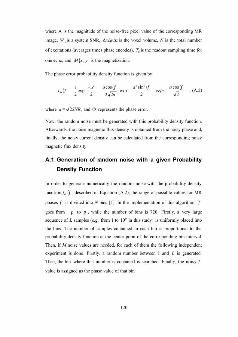
120

where A is the magnitude of the noise-free pixel value of the corresponding MR

image, sΨ is a system SNR, x y z∆ ∆ ∆ is the voxel volume, N is the total number

of excitations (averages times phase encodes), ST is the readout sampling time for

one echo, and ( ),M x y is the magnetization.

The phase error probability density function is given by:

( ) ( ) ( ) ( )2 22 cos sin cos1exp exp

2 2 22 2 2

a a aaf erfc

φ φ φφ

πΦ

− − −= +

, (A.2)

where 2a SNR= , and Φ represents the phase error.

Now, the random noise must be generated with this probability density function.

Afterwards, the noise magnetic flux density is obtained from the noisy phase and,

finally, the noisy current density can be calculated from the corresponding noisy

magnetic flux density.

A.1. Generation of random noise with a given Probability

Density Function

In order to generate numerically the random noise with the probability density

function ( )f φΦ described in Equation (A.2), the range of possible values for MR

phases φ is divided into N bins [1]. In the implementation of this algorithm, φ

goes from π− to π , while the number of bins is 720. Firstly, a very large

sequence of L samples (e.g. from 1 to 106 in this study) is uniformly placed into

the bins. The number of samples contained in each bin is proportional to the

probability density function at the center point of the corresponding bin interval.

Then, if M noise values are needed, for each of them the following independent

experiment is done. Firstly, a random number between 1 and L is generated.

Then, the bin where this number is contained is searched. Finally, the noisy φ

value is assigned as the phase value of that bin.

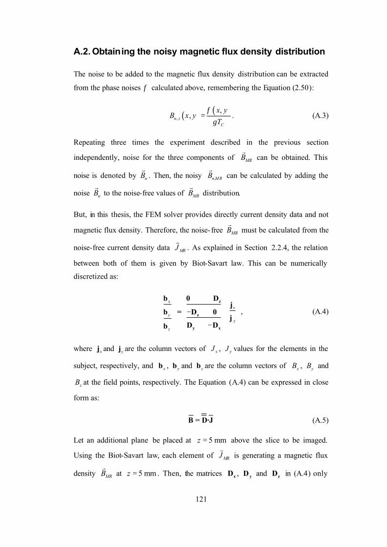
121

A.2. Obtaining the noisy magnetic flux density distribution

The noise to be added to the magnetic flux density distribution can be extracted

from the phase noises φ calculated above, remembering the Equation (2.50):

( ) ( ),

,,n z

C

x yB x y

Tφ

γ= . (A.3)

Repeating three times the experiment described in the previous section

independently, noise for the three components of MRBr

can be obtained. This

noise is denoted by nBr

. Then, the noisy ,n M RBr

can be calculated by adding the

noise nBr

to the noise-free values of MRBr

distribution.

But, in this thesis, the FEM solver provides directly current density data and not

magnetic flux density. Therefore, the noise-free MRBr

must be calculated from the

noise-free current density data MRJr

. As explained in Section 2.2.4, the relation

between both of them is given by Biot-Savart law. This can be numerically

discretized as:

x

x

yy

z

− −

z

z

y x

b 0 Dj

b = D 0j

D Db

, (A.4)

where xj and yj are the column vectors of xJ , yJ values for the elements in the

subject, respectively, and xb , yb and zb are the column vectors of xB , yB and

zB at the field points, respectively. The Equation (A.4) can be expressed in close

form as:

B = D·J (A.5)

Let an additional plane be placed at 5 mmz = above the slice to be imaged.

Using the Biot-Savart law, each element of MRJr

is generating a magnetic flux

density MRBr

at 5 mmz = . Then, the matrices xD , yD and zD in (A.4) only

122

depend on the distance between the elements on the slice and the ones on the

additional plane, and the direction of the vector which connects them.

Consequently, the noise-free MRBr

values can be obtained from the noise-free

MRJr

solving the Equation (A.5).

Now, the noisy magnetic flux density ,n M RBr

can be calculated by adding the

noise nBr

values to the noise-free MRBr

distribution as follows:

,n M R MR nB B B= +r r r

(A.6)

A.3. Obtaining the noisy current density distribution

Finally, once the noisy ,n M RBr

has been calculated, the noise current

density, ,n MRJr

, can be obtained using the inverse of D matrix, as follows:

1−

n,MRn,MRJ = D ·B (A.7)

It is noticeable that, in the noise model of Scott et al, the phase error and the

noise in ,n M RBr

is independent of the noise-free MRBr

values. This means that, for

an increased amount of current density, since MRBr

is also increased, the

proportional noise in the ,n M RBr

values is reduced. Similarly, in such a case, the

proportional noise in ,n MRJr

is also reduced.

Consequently, this model permits the comparison of different current injection

strategies under the same noise conditions. This provides a more realistic and

experimentally verified noise probability density function into the simulations, as

opposed to, for example, making the noise just proportional to the current

magnitude of MRJr

.