estimation of the rock deformation modulus and...
TRANSCRIPT

1
Estimation of the rock deformation modulus and RMR based on Data Mining techniques
Francisco F. Martins
1, Tiago F. S. Miranda
2
ABSTRACT: In this work Data Mining tools are used to develop new and innovative models
for the estimation of the rock deformation modulus and the Rock Mass Rating (RMR). A
database published by Chun et al. (2008) was used to develop these models. The parameters of
the database were the depth, the weightings of the RMR system related to the uniaxial
compressive strength (UCS), the rock quality designation (RQD), the joint spacing (JS), the
joint condition (JC), the groundwater condition (GWC) and the discontinuity orientation
adjustment (DOA), the RMR and the deformation modulus. As a modelling tool the R program
environment was used to apply these advanced techniques. Several algorithms were tested and
analysed using different sets of input parameters. It was possible to develop new models to
predict the rock deformation modulus and the RMR with improved accuracy and, additionally,
allowed to have an insight of the importance of the different input parameters.
Keywords: Deformation modulus; RMR; Data Mining; Machine Learning.
1 Associate Professor, University of Minho, Department of Civil Engineering, School of
Engineering, Campus de Azurém 4800-058 Guimarães, Portugal. E-mail: [email protected].
Tel.: +351 253 510 202. Fax : +351 253 510 217. (Corresponding author)
2 Assistant Professor, University of Minho, Department of Civil Engineering, School of
Engineering, Campus de Azurém 4800-058 Guimarães, Portugal. E-mail:
2
1 Introduction
The deformability modulus (Em) is an important input parameter in any rock mass behaviour
analysis. For a more correct definition of E, considering all factors which govern deformation
behaviour of the rock mass, large scale in situ tests are needed. However, they can be very time
consuming and expensive, and their reliability can be sometimes doubtful (Hoek, E. and
Diederichs, M. (2006).
In this context, most procedures used to estimate this parameter for isotropic rock masses are
based on simple expressions related to the empirical systems, mainly the Rock Mass Rating
(RMR), the Q index and the Geological Strength Index (GSI). Additionally other expressions
can be found which use other index values like the RQD ( Zhang, L. and Einstein, H. 2004) and
the intact rock modulus - Ei (Mitri et al. 1994; Sonmez et al. 2006; Carvalho 2004).
However, defining what kind of E to which these equations lead is important. Most authors
have based their expressions on field test data reported by Serafim and Pereira (1983) and
Bieniawski (1978) and, in some cases, by Stephens and Banks (1989). They mostly refer to the
secant modulus, typically for deformations corresponding to 50% of the peak load. This
deformation is normally higher than the serviceability levels of most geotechnical works built in
rock masses. Thus, these expressions are expected to provide conservative estimates of E.
Nowadays, the use of these expressions is widespread due to their straightforward use.
However, as it should be expected, considerable differences between computed and real values
can be found in many cases. Thus it is important to improve the way these predictions are
carried out in order to obtain more reliable predictions.
In the last decades, new tools of computer sciences and statistics have been developed. Data
Mining (DM) is a relatively new area of computer science which combines different
computational techniques to provide a deeper knowledge about data present in a database. DM
is thus emerging as a class of analytical techniques that go beyond statistics and concerns with
automatically find, simplify and summarize patterns and relationships within a data set.

3
Recently, Chun et al. (2008) presented models based on multiple and polynomial regression
analyses in order to predict Em that included as independent variables the Depth and the RMR
parameters namely: unconfined compressive strength (UCS); Rock Quality Designation (RQD);
joint spacing (JS), joint condition (JC), ground water conditions (GWC); and discontinuity
orientation adjustment (DOA). Their database consisted of 61 collected data sets from road and
railway construction sites in Korea.
This paper introduces an alternative approach based on DM techniques. Several models were
developed with the same database presented by Chun et al. (2008) and are analysed and
compared with the results presented in their work. Different algorithms were used namely
Multiple Regression (MR), Artificial Neural Networks (ANN), Support Vector Machines
(SVM), Regression Trees (RT) and k-Nearest Neighbours (k-NN).
After the analysis of the dataset, a brief description of DM, previous applications in
geotechnical engineering and the applied algorithms is carried out. Afterwards, a first
comparison between the results of the application of several empirical solutions based on the
RMR index to predict Em is carried out based on real in situ results presented by Chun et al.
(2008). Finally, the results of the DM models are presented and analysed.
Furthermore, the same database was used to develop models for the prediction of the RMR
index using less parameters than the original formulation. The main goal was to develop models
which allowed to predict this important index when less information is available, for instance in
the initial stages of a project.
2 Data Mining
2.1 Definition and applications in geotechnical engineering problems
The overall process of discovering useful knowledge from databases is called Knowledge
Discovery in Databases (KDD). In this process, DM is a step related to the application of
specific algorithms for extracting models from data (Fayyad et al. 1996). The KDD process can

4
be resumed in five main steps: data selection, pre-processing, transformation, DM and
interpretation. DM is just a step in this process concerning the application of suitable algorithms
to extract knowledge from data.
Thus, DM is an area of computer science that lies at the intersection of statistics, machine
learning, data management and databases, pattern recognition, artificial intelligence and other
areas. DM allows finding trends and relationships between variables with the objective of
predicting their future state.
Even though their potentialities the use of DM techniques is not yet widespread in
geotechnical engineering. Some examples of DM applications in geotechnical engineering
include: classification of sub-surface soil characteristics using measured data from Cone
Penetration Test applying Decision Trees (DT), Artificial Neural Networks (ANN) and Support
Vector Machines (SVM) (Bhattacharya and Solomatine 2005); soil slope stability prediction
based on field data (Zhou et al. 2002; Souza 2004; Sakellariou and Ferentinou, M. 2005);
identification of probable failure on rock masses based on ANN (Guo et al. 2003); rock
classification using ANN (Millar et al. 1994); modelling of rock deformability behaviour using
ANN (Zhang et al.1991); prediction of maximum surface settlement due tunneling in soft
ground using ANN (Suwansawat and Einstein 2006).
2.2 Used DM Algorithms
The DM algorithms used in this study were the Regression Trees (RT), Multiple Regression
(MR), Artificial Neural Networks (ANN), Support Vector Machines (SVM) and k-Nearest
Neighbours (k-NN). Only the MR provides an equation relating the output variable and the
input variables. A brief explanation of these algorithms is presented in the following paragraphs.
Further details can be found in many publications. Breiman et al. (1984) and Berk (2008) for
RT; Aleksander and Morton (1990) and Ilonen et al. (2003) for ANN; Vapnik (1998),
Cristianini and Shawe-Taylor (2000) and Dibiki et al. (2001) for SVM; Cover (1968) and Cover

5
and Hart (1967) for k-NN.
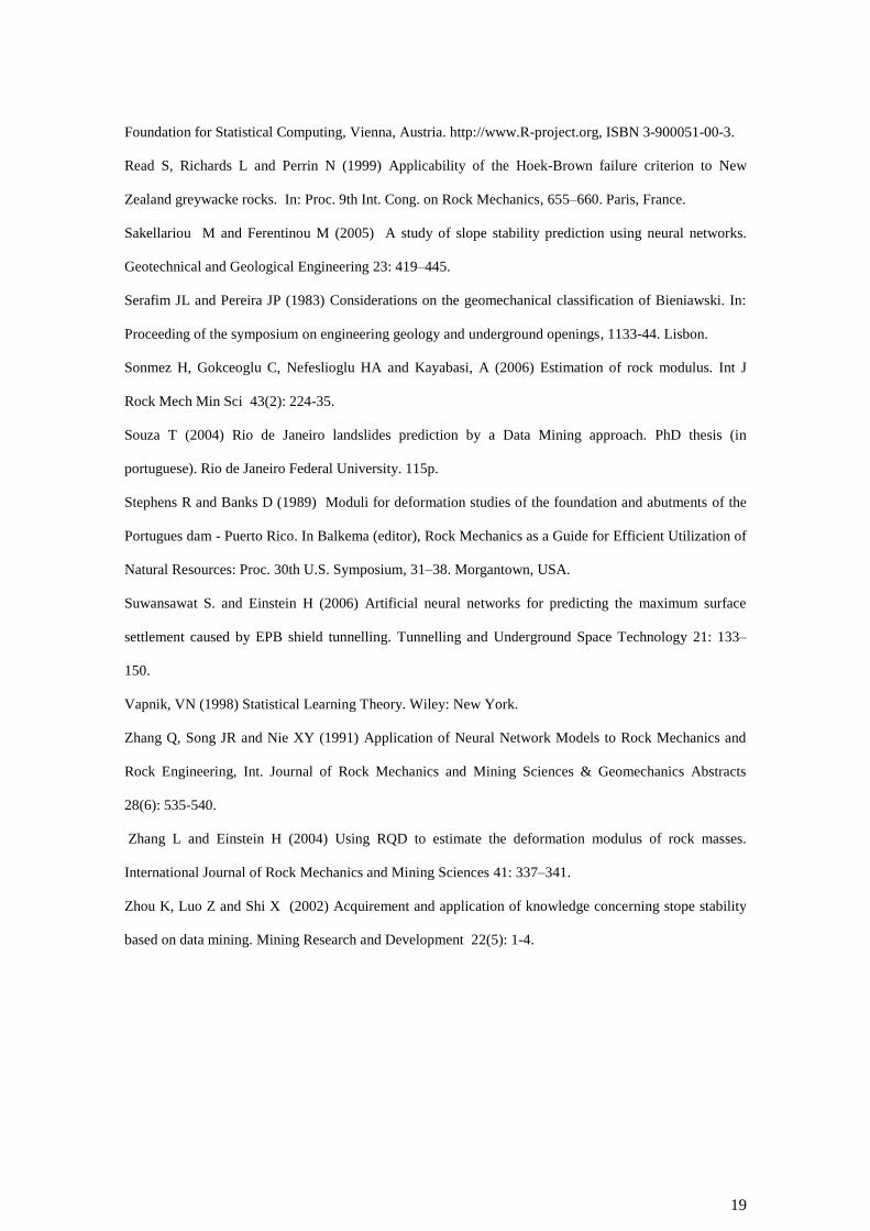
A Decision Tree is an algorithm with a tree structure where a test based on attributes is
established at each node of the tree (Quinlan 1986). Falling branches from each node represent
possible values for the attributes. These trees are denominated Regression Trees (RT) when they
perform the prediction for the value of a continuum variable (Fig. 1).
The MR is quite similar to the simple regression. The main difference is the number of
independent variables involved. The simple regression involves only one independent variable
whereas the MR involves several independent variables and establishes a relationship among
them and the dependent variable.
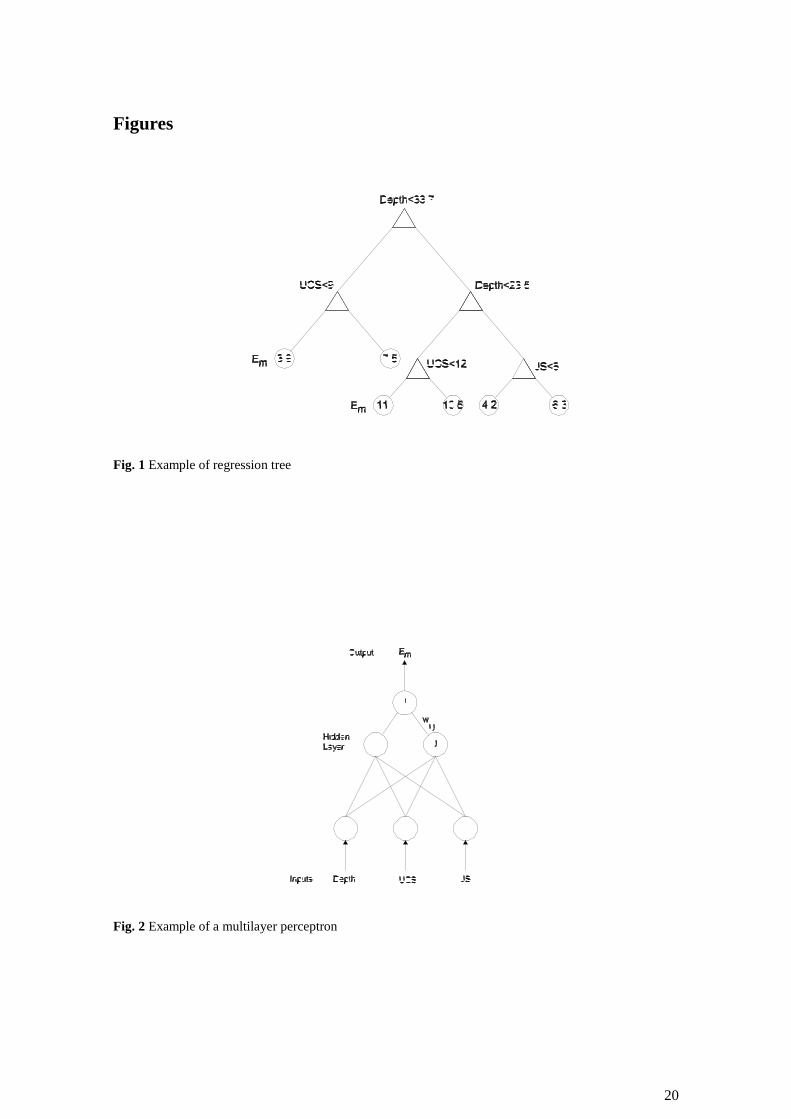
The ANN uses an architecture very close to the human brain structure and is composed of
simple processing units, denominated nodes or artificial neurons, with a large number of
interconnections. The multilayer perceptron architecture was adopted in this work (Haykin
1999) (Fig. 2). The artificial neuron is composed of three main elements: connections set, an
integrator and the level of neuron activation. Each link has an associated weight (wi.j) which is
positive for excitation connections and negative for inhibitory connections. The integrator
reduces the n input arguments, also denominated stimulus, to a single value. The level of neuron
activation is determined by an activation function which controls the output signal, inserting a
non-linear component in the computational process. In this work the weights are randomly
generated in the range [-0.7; +0.7], the base network has one hidden layer of HN hidden nodes
and the activation function is the logistic function (1/(1+exp(-x))). In the training algorithm an
iterative process is applied and the weights are fitted until the error slope approaches zero or
after a maximum number of iterations.
The SVM (Cortes and Vapnik 1995) were originally used in classification problems. The
basic idea was to separate two classes of objects using a set of functions (Fig. 3). This process is
called mapping and the functions are known as kernels. The planes that separate the classes are
known as hyperplanes and there is an optimization iterative algorithm to find the hyperplane
which establishes the largest separation between classes. The vectors placed at the nearest

6
distance in both sides of the hyperplane are denoted support vectors. Both in classification and
regression methods there is an error function to minimize subjected to some constraints.
The kernel functions can be linear, polynomial, sigmoid and radial basis. The Radial Basis
Function is used in this work (Cortez 2010):
0,exp),(2
yxyxk (1)
In addition to the parameter of the kernel, γ, two more parameters are used: the penalty
parameter, C, and an error called ε-insensitive loss function.
The k-NN (Hechenbichler and Schliep 2004) is a quite simple algorithm used in machine
learning both in classification and regression analyses. In both analyses the classification or
value of an object is influenced by the known classifications or values of its nearest neighbours.
The parameter k is the number of neighbours to be considered in the analysis. To search the
vicinity of the objects it is necessary to measure the distance between them. This distance is
computed from position vector in a multidimensional feature space. In regression analysis the
value assigned to the object is a weighted mean value of the k-nearest neighbours’ values. The
optimal value of k can be obtained, for example, through cross validation.
Fig. 4 is presented to explain k-NN in a rather simple way. It shows a simple example of a
classification problem with two classes of objects: “circles” and “squares”. Two circles are
drawn. The inner circle contains the 4 nearest neighbours whereas the outer circle contains the
11 nearest neighbours. For the inner circle, since the number of “circles” (3) is greater than the
number of “squares” inside it, k-NN will assign a “circle” to the outcome of the query instance.
However, for the outer circle the query instance must be classified as “square” because inside it
the number of “squares” is equal to 6 and the number of “circles” is equal to 5.
7
3 Materials and Methods
3.1 Analysis of the dataset
The database used in this work was presented by Chun et al. (2008) and was composed of 61
data sets collected from road and railway construction sites in Korea. The authors used this
database to develop multiple and polynomial regression models to predict Em. The independent
variables present in the database are the Depth and the RMR parameters (UCS, RQD, JS, JC,
GWC and DOA).
The values in the database are quite broad and include almost all spectra of rock mass
qualities. The uniaxial compressive strength ranges from 12.1 MPa to 254.8 MPa. This
parameter only does not include the lower values whose ratings are lower than 2. The ratings of
the Rock Quality Designation (RQD), of the spacing discontinuities (JS) and of the
discontinuity orientation adjustment (DOA) vary from the lower to the higher possible values of
the Rock Mass Rating System. The joint condition (JC) and the groundwater condition (GWC)
do not include the lower values of the ratings. In conclusion, the database includes almost all
range of rock materials. Only material in the transition from highly weathered rock and soil is
not included. Nonetheless this is not an important issue since the RMR system in not applicable
under these conditions. In Table 1 some statistical attributes from the database are presented.
3.2 Modelling and evaluation
The modelling software was the R program environment (R Development Core Team 2010)
which is an open source freeware statistical package. Within this framework a specific program
RMiner (Cortez 2010) was used which allow applying several algorithms and evaluating their
behaviour under a different set of metrics.
The performance of the different DM models was assessed and compared through the
Regression Error Characteristic (REC) curves and global metrics based on the errors between

8
real and predictive values.
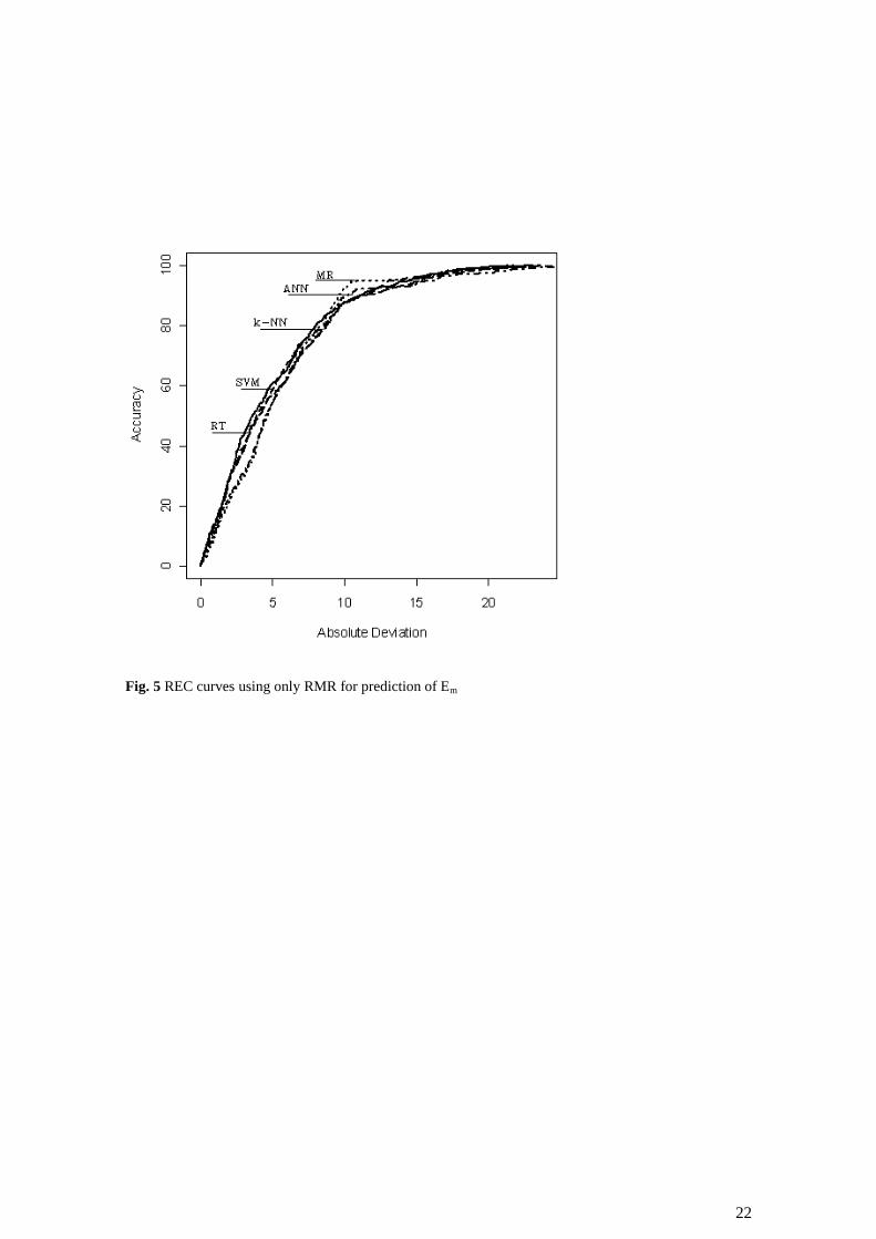
The REC curve (Fig. 5) plots the error tolerance on the x-axis versus the percentage of points
predicted within the tolerance on the y-axis (Bi and Bennett 2003). It is a technique that both
allows the evaluation of regression models and facilitates visual comparison of the performance
of the different models. The best performance is attributed to the model with the larger area
below the curve.
In this work the following global metrics are used: Mean Absolute Deviation (MAD),
Relative Absolute Error (RAE), Root Mean Squared Error (RMSE), Relative Root Mean
Squared Error (RRMSE) and Pearson’s product-moment correlation coefficient (R):
N
1i ii yyN
1MAD
(2)
%100
N
yy
MADRAE
N
1i ii
(3)
N
yyRMSE
N
1i
2ii
(4)
%100
N
yy
RMSERRMSE
N
1i
2ii
(5)
N
1i
2
iN
1i
2i
N
1i ii
yyyy
yyyyR
(6)
where N denotes the number of examples, yi the desired value, iy the estimated value by the
considered model, y the mean of the desired values and y
the mean of the estimated values.
In Data Mining the learning process is based on the application of an algorithm to a set of
records with the aim to obtain a pattern or model which is applicable to new cases.
9
There are several methods to evaluate the algorithm performance. In this paper the cross-
validation (Efron and Tibshirani 1993) was applied which allows the use of all the available
cases. The examples were divided in 5 subsets with approximately equal number of records. Ten
runs were performed using 4/5 of the records for training and 1/5 for testing. The final metrics
are the mean of the metrics of validation obtained in the 10 runs. The confidence interval of the
metrics is based on t – student statistical with a 95% confidence level.
The importance of each input parameter was also evaluated by applying a sensitivity analysis
(Kewley et al. 2000). This analysis is applied after the training phase and is intended to evaluate
the response of the model when the input parameters are changed. The importance of a given
input parameter is evaluated by changing its value from a minimum to a maximum and at same
time maintaining the remaining input parameters with its mean values. A parameter with a
strong influence in the model induces a high variance in the model output whereas a parameter
with low importance induces a short variance.
3.3 Comparison between predictive models based only on RMR
The first part of this study consisted on a comparison between the predictions of different
correlations that can be found in literature which use the RMR index to predict Em. The RMR
values within the database were used to compute the predictions of E and these predictions were
compared with the real values in the database. The correlations used in this comparative study
and the main results are presented in Table 2. In this study the correlations that use the elastic
modulus of the intact rock were not included since the direct measurement of this parameter was
not available.
The performance of the different correlations is assessed by the metrics MAD and RMSE and
parameters of the plot predicted versus real Em values namely the slope of the trend line (a) and
the square of the Pearson’s correlation coefficient (R2).
The best results can be considered to be found for the correlation by Chun et al. (2008). This

10
fact was expected since this expression was developed using the present database. Nonetheless,
the results are poor mainly translated by the low value of R2 and considerably high error values.
This evaluation demonstrates the limited extrapolation capacity of the correlations based only
on the RMR index mostly in cases outside their original database. In this sense these
expressions should only be used to get a first preliminary approach for the Em prediction.
The next step was the application of the DM techniques to analyse the possibility of
developing more accurate models for the Em prediction based only on the same index. The idea
was to check if it was possible to improve predictions based on only one parameter. The REC
curves for all models are presented in Fig. 5. It can be seen that all the models have a similar
performance. However, comparing the global metrics given in Table 3, the k-NN model has
slightly better performance.
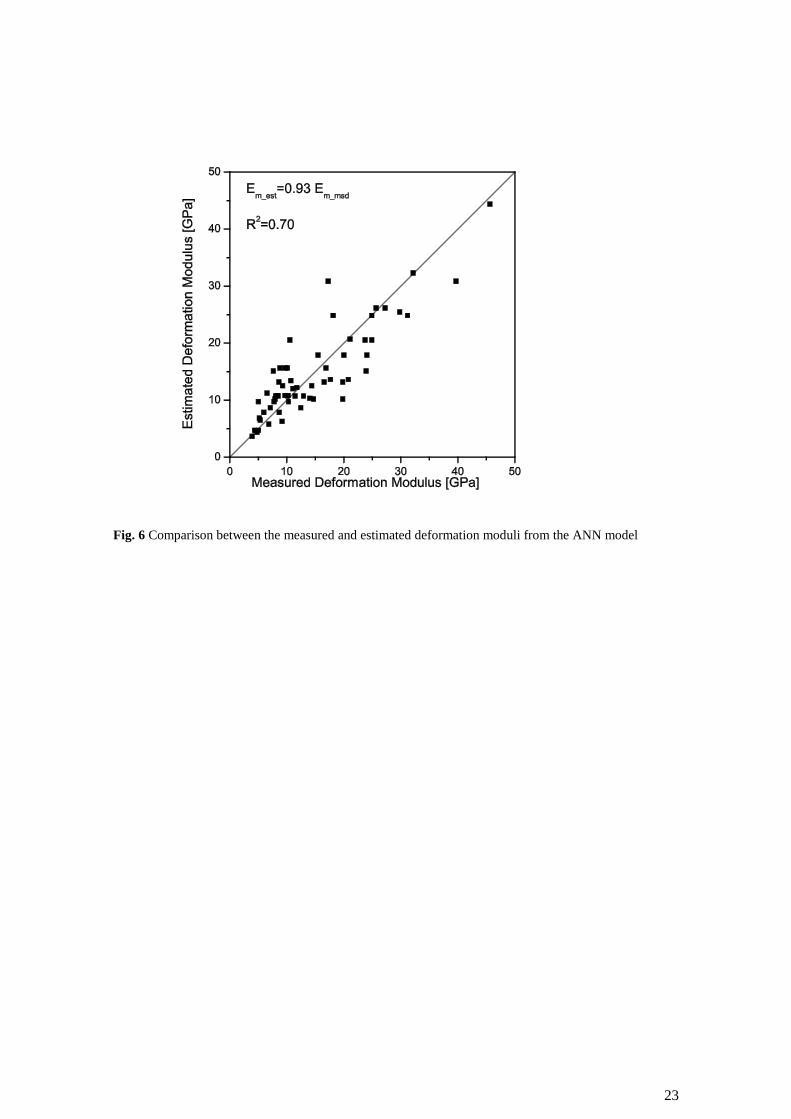
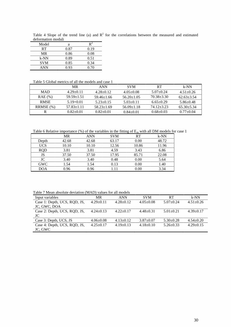
The results presented in Table 3 were computed using the cross-validation methodology
previously presented and is used to compute the overall accuracy of the models. To obtain the
final model all the data is then used to induce the final models. Table 4 presents the slope of the
trend line (a) and the square of the Pearson’s correlation coefficient (R2) for the correlations
between the measured and estimated deformation moduli for the models including all the data.
The best results are observed for the ANN model with a slope value near the unity (Fig. 6) and a
R2 which is considerably higher than the best results of the correlations (0.54). These results
show that using the DM techniques it was possible to develop more accurate predictive models
for Em based on a single index, in this case the RMR, in comparison with the correlations
normally used. However, the results are not as reasonable as desired.
3.4 Predictive models for several combinations of input variables
A simple correlation between Em and RMR is always a simple model with limited predictive
accuracy. However, the RMR resumes a great quantity of geotechnical information in a single
index. A correlation between RMR and Em considers the underlying principle that each

11
parameter constituting the system has identical correlation strength to predict Em which is a
limitation. The next study intended to test the capacity of the DM algorithms to predict Em using
the different parameters that constitute the RMR separately. This would also allow checking the
relative importance of each in the deformability prediction of a rock mass.
In this sense several combinations of the input variables were used. The first case (case 1)
includes all the input variables given in Table 1, except RMR. Fig. 7 shows the REC curves
obtained for this case. According to this figure there are three models with a similar
performance (ANN, SVM and MR). This fact can be confirmed analysing the global metrics
given by equations (2) to (6) (Table 5). The SVM model presents the best global metrics and
therefore has the best predictive capacity.
Fig. 8 shows the comparison between the measured and estimated deformation moduli for the
SVM model and case 1.
Table 6 shows the importance of the variables according to different models for case 1 which
differs from model to model. However, the three most important input variables for almost all
models are the Depth, JS and UCS. The other variables have relatively low impact in the
models. It is then important to point out the significant importance of Depth that can be related
with in situ state of stress, in the prediction of Em. The original formulation of RMR does not
take into account this parameter which can be considered a drawback of this system. The
importance of UCS and JS in the deformability of a rock mass was expected and is
understandable.
It is quite surprising that GWC and DOA have a minor influence on Em. It is known that an
increase in water content can reduce the value of Em and the discontinuity orientation may
influence the value of Em. However, it must be stressed that the models used to adjust the data
depend on the used dataset. Chun et al. (2008) established correlation between the Em and each
input parameter, except DOA. They concluded that, for the used database, the effect of ground
water on the deformation modulus is negligible. The R2 between Em and GWC is almost zero
(0.001). That’s why they excluded the ground water in their polynomial regression (Eq. 7).

12
Establishing a correlation between Em and DOA a very poor correlation is obtained (R2=0.03).
Therefore, it seems correct the importance given by the models to GWC and DOA.
Taking into account these results and the independent variables used in the best correlation
obtained by Chun et al. (2008) (Eq. (7)), three more analyses were carried out (cases 2 to 4).
The input variables for case 2 were Depth, UCS, RQD, JS and JC, for case 3 were Depth, UCS
and JS, and for case 4 were Depth, UCS, RQD, JS, JC and GWC.
10000
JC530.2399JS031.0RQD851.4UCS83.1Depth992.5]GPa[E
5342
est_m
(7)
Tables 7 and 8 show the analysed cases so far and lists the performance of the models in
terms of MAD and R, respectively. Generally, the SVM models yield lower errors and greater R
whereas the RT models yield greater errors and lower R. The only exception is for case 2, where
the SVM model has not the best performance. Case 3, with only three input variables, yields
lower errors than the other cases for MR, ANN and SVM models. As the MR model has a close
performance to the SVM model and is simpler than this one it constitutes a good alternative.
The MR model can be represented by a simple linear equation, which for case 3 is the
following:
JSUCSDepthGPaE estm 1458.16435.01005.01372.8][_ (8)
A comparison between the measured and estimated results from Eq. (8) is shown in Fig. 9.
The correlation coefficient between the estimated and measured Em is 0.83 and the slope of
trend line is 0.93, showing nearly a 1:1 slope and pointing out for a good behaviour of the
model. However, shortcomings arise when Eq. (8) is used for the combination of low values of
the three input variables. As the intercept value is negative the value obtained for the
deformation modulus can be negative.

13
Applying all the data to induce the final models for cases 2 and 3, the best results were
obtained with the SVM model. The comparison between the measured and estimated Em for this
algorithm shows a good correlation (Figs. 10 and 11). The regression line passes through the
central part of the dataset in Figs. 10 and 11, and the slopes of the trend lines are close to a 1:1
correlation. The coefficients of correlation, R, are 0.88 and 0.89 for case 2 and case 3,
respectively.
These results are very close to the best correlation obtained by Chun et al. (2008) whose
correlation has a=0.95 and R2=0.79. Nevertheless, case 3 only uses three input variables instead
of the five input variables used in case 2 and by Chun et al.(2008). This fact can be important
mainly in the preliminary design stages where information about the rock mass is scarce and
uncertain.
Two more cases were tested which were similar to cases 2 and 3 where the logarithm of Em is
used to prevent negative values of this parameter to be predicted. These cases are denoted by
cases 5 and 6. Case 5 includes Depth, UCS, RQD, JS and JC as input variables and case 6
includes Depth, UCS and JS. The MAD and R values for these cases are presented in Tables 9
and 10.
Using all dataset to induce the final models for cases 5 and 6, the best results were obtained
with the ANN and SVM models, respectively. The comparison between the measured and
estimated Em for these algorithms (Figs. 12 and 13) shows a slightly poorer correlation than
those obtained in Figs. 10 and 11.
3.5 RMR Prediction
It was observed in the previous study that the different input parameters of the RMR index had
significant different importance in the Em prediction. In this context it was decided to explore
this issue by using the DM techniques to predict RMR which would allow checking the relative
importance of each parameter and developing predictive models for RMR using less
information than the original formulation.

14
As it was done concerning Em, the experiments were performed using a number of different
input parameters to assess the models performance. The first analysed case (case 7) includes all
the attributes given in Table 1, except Em. Fig. 14 shows the obtained REC curves. According to
Fig. 14 the most suitable models to predict RMR are the MR and ANN models. However,
analysing Table 11 it can be concluded that the ANN model is the most accurate one.
Table 12 shows the importance of the variables according to different models for case 7. The
most important variables to predict RMR are RQD, JS, JC and DOA, with values greater than
10% each. It is interesting to notice that the most important parameters are the ones related with
the rock mass jointing. A similar conclusion was reached by Miranda et al. (2008) on a similar
study but in a different and large database of 1230 cases of application of the RMR system in a
granite rock mass. These results point out to the direct and strict relation between jointing
conditions and overall rock mass quality.
Taking into account these results and the need to use less parameters than those used in the
RMR system, two more analyses were carried out (cases 8 and 9). Tables 13 and 14 show the
results for these cases and list the performance of the models in terms of MAD and R,
respectively. For case 8 the ANN and MR models give the best performances, whereas for case
9 the SVM model is the most accurate.
Using all the data for cases 8 and 9 the best results were obtained with the ANN model (case
8) and the k-NN model (case 9). The comparison between the calculated and estimated RMR
values is shown in Figs. 15 and 16. Since the MR model provides good results, with the
advantage of being simple to use, it is worthwhile to present its equations for cases 8 and 9:
DOA162.1JC237.1JS273.1RQD202.1774.9RMR (9)
JC1404.1JS5947.0RQD2249.16314.10RMR (10)
15
4 Conclusions
Using a database of geotechnical data published by Chun et al (2008) DM techniques were
applied in order to develop new models to predict Em and RMR. The DM algorithms used in this
study were the Regression Trees (RT), Multiple Regression (MR), Artificial Neural Networks
(ANN), Support Vector Machines (SVM) and k-Nearest Neighbours (k-NN). The main results
that can be drawn from this study are described in the following items:
Simple correlations based only on the RMR provide rough predictions of Em mostly
when extrapolating to cases outside the original database based on which they were
developed. Therefore they should only be used for a preliminary approach. Using the
DM algorithms it was possible to develop more accurate predictive models using only
the RMR index, namely with the ANN algorithm. However, even though the
improvement of the results the associated errors were still considerably high.
Using the DM techniques with several sets of parameters to predict Em the results were
highly improved. In most cases the ANN and the SVM algorithms showed the best
performance. Also the MR models can be considered good alternatives because they are
simple to use and implement and provide good results.
The most important input variables to predict Em for almost all the models were Depth,
JS and UCS. The first parameter can be related to the in situ state of stress which is not
taken into account in the original formulation of the RMR and can be considered a
drawback of this system. The high importance of the remaining variables was expected.
The input variables GWC and DOA have very low importance in the prediction of Em.
This could be considered quite surprising. However, the same conclusion was obtained
by Chun et al (2008). It must be emphasized the dependence of the models on the used
database.
Comparing the results to those obtained by Chun et al. it was concluded that they are
similar. However, using the DM techniques it was possible to induce models using less
16
input parameters than those by Chun et al.
The SVM model using only three input parameters (Depth, JS and UCS) has an
excellent predictive capacity of the Em and is the best alternative to the Chun et al.
solution.
Using the same database the DM techniques were applied to induce prediction models
for the RMR that could use less information than the original formulation. Different
combinations of input parameters were used and the most suitable models to predict
RMR were the MR and the ANN models which presented a very good performance.
The most important input parameters to predict RMR were RQD, JS, JC and DOA
which are the ones related with jointing of the rock mass. This fact corroborates the
conclusion of a previous study by Miranda et al. (2008) and indicates a very close
relation between jointing conditions and overall rock mass quality.
The ANN model using only the above four input parameters is recommended to
estimate RMR.
Given the high quality of results obtained with the DM techniques, the next step is to
test the models with larger databases based on practical examples.
Acknowledgements This study has been carried out under the framework of the strategic plan (2011-2012) of
Territory, Environment and Construction Centre (C-TAC/UM), PEst-OE/ECI/UI4047/2011,
approved by the Portuguese Foundation for Science and Technology (FCT).
References
Aleksander I and Morton H (1990) An Introduction to Neural Computing. Chapman & Hall.
Berk, RA (2008) Statistical Learning from a Regression Perspective. Springer Series in Statistics. New
York: Springer-Verlag.
Bhattacharya B, Solomatine, D (2005) Machine Learning in Soil Classification. In: Proc. of Int. Joint

17
Conf. on Neural Networks, Montreal, Canada.
Bieniawski ZT (1978) Determining rock mass deformability: experience from case histories. Int J Rock
Mech Min Sci Geomech Abstr. 15: 237-47.
Bi J and Bennett K (2003) Regression Error Characteristic curves. In: Proceedings of 20th Int. Conf. on
Machine Learning (ICML), Washington DC, USA.
Breiman L, Friedman JH, Olshen RA and Stone CJ (1984) Classification and Regression Trees.Chapman
& Hall/CRC.
Carvalho J (2004) Estimation of rock mass modulus. Personal communication.
Chun B-S, Ryu WR, Sagong M, Do J-N (2008) Indirect estimation of the rock deformation modulus
based on polynomial and multiple regression analyses of the RMR system. Int. J. Rock Mech. Mining
Sciences 46: 649-658.
Cortes C and Vapnik V (1995) Support Vector Networks. Machine Learning 20(3): 273-297. Kluwer
Academic Publishers.
Cortez P (2010) Data Mining with Neural Networks and Support Vector Machines using the R/rminer
Tool, In: P. Perner (Ed.), Advances in Data Mining. Applications and theoretical aspects. Proceedings of
10th Industrial Conference on Data Mining, Berlin, Germany, Lecture Notes in Computer Science,
Springer, 572-583.
Cover TM (1968) Estimation by the nearest neighbor rule. IEEE Transactions on Information Theory
14(1): 50-55.
Cover TM and Hart PE (1967) Nearest neighbor pattern classification, IEEE Transactions on Information
Theory 13(1): 21-27.
Cristianini N, Shawe-Taylor J (2000) An Introduction to Support Vector Machine. University Press,
London, Cambridge.
Dibike YB, Velickov S, Solomatine DP and Abbott MB (2001) Model introduction with support vector
machines; introduction and applications. Journal of Computing in Civil Engineering, American Society of
Civil Engineers (ASCE) 15(3): 208-216.
Efron B and Tibshirani R (1993) An Introduction to the Bootstrap. Chapman & Hall.
Fayyad U, Piatesky-Shapiro G and Smyth P (1996) From Data Mining to Knowledge Discovery: An
Overview. In: Fayyad et al. (eds) Advances in Knowledge Discovery and Data Mining. AAAI Press /
18
The MIT Press, Cambridge MA, 471-493.
Guo L, Wu A, Zhou K and Yao Z (2003) Pattern recognition and its intelligent realization of probable
rock mass failure based on RES approach. Chinese Journal of Nonferrous Metals 13(3): 749-753.
Haykin S (1999) Neural Networks - A Compreensive Foundation. New Jersey: Prentice-Hall, 2nd edition.
Hechenbichler, K. e Schliep, K. 2004. Weighted k-Nearest-Neighbor Techniques and Ordinal
Classification. Discussion Paper 399, SFB 386, Ludwig-Maximilians University Munich. URL:
http://epub.ub.uni-muenchen.de/archive/00001769/01/paper_399.pdf.
Hoek E and Diederichs M (2006) Empirical estimation of rock mass modulus. International Journal of
Rock Mechanics and Mining Sciences 43: 203–215.
Ilonen J, Kamarainen JK, Lampinen J (2003) Differential evolution training algorithm for feed-forward
neural network. Neural Processing Letters 17: 93-105.
Kewley R, Embrechts M and Breneman C (2000) Data strip mining for the virtual design of
pharmaceuticals with neural networks. IEEE Transactions on Neural Networks. 11(3): 668-679.
Kim G (1993) Revaluation of geomechanics classification of rock masses. In: Proceedings of the Korean
geotechnical society of spring national conference, 33-40. Seoul.
Millar DL, Hudson JA (1994) Performance Monitoring of Rock Engineering Systems using Neural
Networks, Transactions of the Institution of Mining and Metallurgy Section A – Mining Industry 103:
A3-A16.
Miranda T (2007) Geomechanical parameters evaluation in underground structures. Artificial
intelligence, Bayesian probabilities and inverse methods. PhD thesis. University of Minho, Guimarães,
Portugal, 291p.
Miranda T, Gomes Correia A. and Ribeiro e Sousa L (2008) Development of new models for
geomechanical characterisation using Data Mining techniques. Geomechanics and Tunnelling 5: 328-
334.
Mitri HS, Edrissi R and Henning J (1994). Finite element modeling of cablebolted slopes in hard rock
ground mines. In: Proceedings of the SME annual meeting, 94-116. Albuquerque.
Quinlan, J. 1986. Induction of Decision Trees. Machine Learning 1: 81-106. Kluwer Academic
Publishers.
R Development Core Team (2010) R: A language and environment for statistical computing. R
19
Foundation for Statistical Computing, Vienna, Austria. http://www.R-project.org, ISBN 3-900051-00-3.
Read S, Richards L and Perrin N (1999) Applicability of the Hoek-Brown failure criterion to New
Zealand greywacke rocks. In: Proc. 9th Int. Cong. on Rock Mechanics, 655–660. Paris, France.
Sakellariou M and Ferentinou M (2005) A study of slope stability prediction using neural networks.
Geotechnical and Geological Engineering 23: 419–445.
Serafim JL and Pereira JP (1983) Considerations on the geomechanical classification of Bieniawski. In:
Proceeding of the symposium on engineering geology and underground openings, 1133-44. Lisbon.
Sonmez H, Gokceoglu C, Nefeslioglu HA and Kayabasi, A (2006) Estimation of rock modulus. Int J
Rock Mech Min Sci 43(2): 224-35.
Souza T (2004) Rio de Janeiro landslides prediction by a Data Mining approach. PhD thesis (in
portuguese). Rio de Janeiro Federal University. 115p.
Stephens R and Banks D (1989) Moduli for deformation studies of the foundation and abutments of the
Portugues dam - Puerto Rico. In Balkema (editor), Rock Mechanics as a Guide for Efficient Utilization of
Natural Resources: Proc. 30th U.S. Symposium, 31–38. Morgantown, USA.
Suwansawat S. and Einstein H (2006) Artificial neural networks for predicting the maximum surface
settlement caused by EPB shield tunnelling. Tunnelling and Underground Space Technology 21: 133–
150.
Vapnik, VN (1998) Statistical Learning Theory. Wiley: New York.
Zhang Q, Song JR and Nie XY (1991) Application of Neural Network Models to Rock Mechanics and
Rock Engineering, Int. Journal of Rock Mechanics and Mining Sciences & Geomechanics Abstracts
28(6): 535-540.
Zhang L and Einstein H (2004) Using RQD to estimate the deformation modulus of rock masses.
International Journal of Rock Mechanics and Mining Sciences 41: 337–341.
Zhou K, Luo Z and Shi X (2002) Acquirement and application of knowledge concerning stope stability
based on data mining. Mining Research and Development 22(5): 1-4.
20
Figures
Fig. 1 Example of regression tree
Fig. 2 Example of a multilayer perceptron

21
Fig. 3 Example of the SVM transformation
Fig. 4 Example of k-NN classification
22
Fig. 5 REC curves using only RMR for prediction of Em
23
Fig. 6 Comparison between the measured and estimated deformation moduli from the ANN model

24
Fig. 7 REC curves for case 1
Fig. 8 Relationship between the measured and estimated deformation moduli from the SVM model for
case 1

25
Fig. 9 Comparison between the measured and estimated deformation moduli from the MR model analysis
(case 3)
Fig. 10 Comparison between the measured and estimated deformation moduli from the SVM model
analysis (case 2)

26
Fig. 11 Comparison between the measured and estimated deformation moduli from the SVM model
analysis (case 3)
Fig. 12 Comparison between the measured and estimated deformation moduli from the NN model
analysis (case 5)

27
Fig. 13 Comparison between the measured and estimated deformation moduli from the SVM model
analysis (case 6)
Fig. 14 REC curves for case 7

28
Fig. 15 Comparison between the calculated and estimated RMR from the ANN model analysis (case 8)
Fig. 16 Comparison between the calculated and estimated RMR from the k-NN model analysis (case 9)

29
Table 1 Some statistics of the data
Atribute Min. 1st
Quartile Median Mean
3rd
Quartile Max.
Standard
Deviation
Depth 4.00 15.00 23.5 33.74 31.00 166.00 36.33
UCS 2.00 9.00 12.00 10.82 13.00 15.00 3.25
RQD 3.00 13.00 17.00 15.58 20.00 20.00 4.64
JS 5.00 8.00 10.00 10.85 13.00 20.00 3.96
JC 9.00 20.00 24.00 22.92 27.00 30.00 5.36
GWC 4.00 7.00 10.00 9.28 10.00 15.00 2.43
DOA -25.00 -10.00 -5.00 -7.18 -5.00 0.00 5.51
RMR 21.0 56.0 64.0 62.3 72.0 92.0 14.47
Em 3.92 8.31 11.08 14.64 19.81 45.62 9.05
Table 2 Empirical correlations for the extrapolation of the in situ deformation modulus based on the RMR
Correlations (Em in GPa) References a R2 MAD RMSE
RMR0364.0exp332.1Em Chun et al. (2008) 0.88 0.37 4.6 5.9
100RMR2Em )50RMR( Bieniawski (1978) 1.93 0.51 16.4 21.2
40/10RMR
m 10E )50RMR( Serafim and
Pereira (1983)
3m 10RMR07.0exp300E Kim (1993) 2.54 0.54 21.8 34.9
3m 10/RMR1.0E Read et al. (1999) 1.75 0.50 13.7 17.2 2388.35
m RMR103E Miranda (2007) 1.47 0.53 12.6 9.6
Table 3 Global metrics of all models using only the RMR
MR ANN SVM RT k-NN
MAD 5.38±0.07 6.12±1.07 5.18±0.19 5.38 ±0.15 5.03±0.20
RAE (%) 74.68±1.0
2 84.95±14.79 71.88±2.63
74.62±2.12 69.80±2.78
RMSE 6.69±0.06 10.73±7.75 6.81±0.34 7.11±0.21 6.65±0.26
RRMSE (%) 74.55±0.6
9 119.59±86.35 75.89±3.80
79.20±2.29 74.09±2.90
R 0.67±0.01 0.59±0.06 0.65±0.04 0.62±0.02 0.68±0.03
30
Table 4 Slope of the trend line (a) and R
2 for the correlations between the measured and estimated
deformation moduli
Model a R2
RT 0.87 0.19
MR 0.86 0.08
k-NN 0.89 0.51
SVM 0.85 0.34
ANN 0.93 0.70
Table 5 Global metrics of all the models and case 1
MR ANN SVM RT k-NN
MAD 4.29±0.11 4.28±0.12 4.05±0.08 5.07±0.24 4.51±0.26
RAE (%) 59.59±1.51 59.46±1.66 56.20±1.05 70.38±3.30 62.63±3.54
RMSE 5.19+0.01 5.23±0.15 5.03±0.11 6.65±0.29 5.86±0.48
RRMSE (%) 57.83±1.11 58.23±1.69 56.09±1.18 74.12±3.23 65.30±5.34
R 0.82±0.01 0.82±0.01 0.84±0.01 0.68±0.03 0.77±0.04
Table 6 Relative importance (%) of the variables in the fitting of Em with all DM models for case 1
MR ANN SVM RT k-NN
Depth 42.68 42.68 63.17 0.00 48.72
UCS 10.10 10.10 12.56 10.86 11.96
RQD 3.81 3.81 4.59 3.43 6.86
JS 37.50 37.50 17.95 85.71 22.08
JC 3.40 3.40 0.48 0.00 5.64
GWC 1.54 1.54 0.13 0.00 1.40
DOA 0.96 0.96 1.11 0.00 3.34
Table 7 Mean absolute deviation (MAD) values for all models
Input variables MR ANN SVM RT k-NN
Case 1: Depth, UCS, RQD, JS,
JC, GWC, DOA
4.29±0.11 4.28±0.12 4.05±0.08 5.07±0.24 4.51±0.26
Case 2: Depth, UCS, RQD, JS,
JC
4.24±0.13 4.22±0.17 4.48±0.31 5.01±0.21 4.39±0.17
Case 3: Depth, UCS, JS 4.06±0.08 4.13±0.12 3.87±0.07 5.30±0.28 4.54±0.20
Case 4: Depth, UCS, RQD, JS,
JC, GWC
4.25±0.17 4.19±0.13 4.18±0.10 5.26±0.33 4.29±0.15

31
Table 8 Pearson’s product-moment correlation (R) for all models
Input variables MR ANN SVM RT k-NN
Case 1: Depth, UCS, RQD, JS,
JC, GWC, DOA
0.82±0.01 0.82±0.01 0.84±0.01 0.68±0.03 0.77±0.04
Case 2: Depth, UCS, RQD, JS,
JC
0.83±0.01 0.83±0.02 0.77±0.04 0.68±0.03 0.78±0.04
Case 3: Depth, UCS, JS 0.84±0.01 0.83±0.01 0.86±0.00 0.64±0.05 0.77±0.03
Case 4: Depth, UCS, RQD, JS,
JC, GWC
0.82±0.02 0.82±0.01 0.82±0.02 0.64±0.05 0.79±0.02
Table 9 Mean absolute deviation (MAD) for all models
Input variables MR ANN SVM RT k-NN
Case 5: Depth, UCS, RQD, JS,
JC
0.12±0.00 0.12±0.00 0.12±0.00 0.17±0.01 0.14±0.00
Case 6: Depth, UCS, JS 0.12±0.00 0.12±0.00 0.13±0.01 0.17±0.01 0.14±0.01
Table 10 Pearson’s product-moment correlation (R) for all models
Input variables MR ANN SVM RT k-NN
Case 5: Depth, UCS, RQD, JS,
JC
0.84±0.01 0.84±0.00 0.84±0.01 0.64±0.04 0.14±0.00
Case 6: Depth, UCS, JS 0.82±0.01 0.82±0.01 0.81±0.02 0.60±0.04 0.76±0.02
Table 11 Global metrics for all DM models
MR ANN SVM RT k-NN
MAD 0.13±0.01 0.12±0.00 0.64±0.06 7.30±0.73 4.08±0.16
RAE (%) 1.17±0.05 1.13±0.04 5.80±0.50 66.57±6.68 37.21±1.43
RMSE 0.19±0.01 0.18±0.01 1.08±0.15 9.21±0.93 5.55±0.25
RRMSE
(%)
1.33±0.05 1.27±0.05 7.52±1.04
64.17±6.47 38.67±1.73
COR 1.00±0.00 1.00±0.00 1.00±0.00 0.77±0.05 0.93±0.01

32
Table 12 Relative importance (%) of the variables in the fitting of RMR with the main DM models for case 5
RT MR ANN SVM k-NN
Depth 0.00 0.00 0.00 0.21 11.42
UCS 0.00 8.96 8.96 9.29 7.51
RQD 89.88 15.61 15.61 16.34 23.49
JS 0.00 12.12 12.12 13.35 17.42
JC 10.12 23.40 23.40 23.43 26.08
GWC 0.00 6.48 6.48 6.72 8.87
DOA 0.00 33.43 33.43 30.67 5.22
Table 13 Mean absolute deviation (MAD) values for all models
Input variables MR ANN SVM RT k-NN
Case 7: Depth, UCS, RQD,
JS, JC, GWC, DOA
0.13±0.01 0.12±0.00 0.64±0.06 7.30±0.73 4.08±0.16
Case 8: RQD, JS, JC, DOA 2.73±0.04 2.75±0.06 2.88±0.08 7.23±0.32 4.32±0.19
Case 9: RQD, JS, JC 5.71±0.14 5.78±0.25 5.41±0.17 7.06±0.39 5.57±0.14
Table 14 Pearson’s product-moment correlation coefficients (R) for all models
Input variables MR ANN SVM RT k-NN
Case 7: Depth, UCS, RQD,
JS, JC, GWC, DOA
1.00±0.00 1.00±0.00 1.00±0.00 0.77±0.05 0.93±0.01
Case 8: RQD, JS, JC, DOA 0.97±0.00 0.97±0.00 0.96±0.00 0.78±0.02 0.92±0.01
Case 9: RQD, JS, JC 0.86±0.01 0.86±0.01 0.86±0.01 0.79±0.03 0.86±0.01