Estimation and Analysis of the Deformation of the Cardiac Wallusing Doppler Tissue Imaging.

Valerie Moreau��� �

Laurent D. Cohen�

Denis Pellerin�

�CEREMADE Universite Paris 9 Dauphine, 75775 Paris cedex 16, France�

now with Epidaure project at INRIA Sophia Antipolis�Saint George’s Hospital, London, UK.

E-mail: moreau,cohen@ceremade.dauphine.fr, dpellerin@sghms.ac.uk

Abstract

This paper presents different ways to use the DopplerTissue Imaging (DTI) in order to determine deformation ofthe cardiac wall. As an extra information added to the ul-trasound images, the DTI gives the velocity in the direc-tion of the probe. We first show a way to track points alongthe cardiac wall in a M-Mode image (1D+t). This is basedon energy minimization similar to a deformable grid. Wethen extend the ideas to finding the deformation field in asequence of 2D images (2D+t). This is based on energyminimization including spatio-temporal regularization.

1 Introduction

Doppler Tissue Imaging (DTI) is a recent non invasiveultrasound technique which allows to measure the veloc-ity of intramyocardial wall motion. Results consists of acolor overlay superimposed to the grey-scale conventionalimage (see Figure 1). At first the frame rate and the tempo-ral resolution did not allow a precise study of the cardiacwall velocities over a whole cardiac cycle. That is whycardiologists need M-mode images (bottom of Figure 1).In practice, the cardiologist chooses a segment on the 2Dimage and the M-mode image shows its evolution throughtime. Each column of the image

�������� corresponds to the

segment at a given time�. Whereas a 2D sequence acquired

with our VINGMED ultrasound system consists of about100 images per second, an M-mode image consists of morethan 500 frames per second.

This work follows the work performed by the authors of[1] about M-mode images. This work consists of trackingthe cardiac wall with a variant of active contours. The con-tour � ���� �������������� �

deforms to minimize������ ������ �!#"%$ �'& $ (*)+! ( $ �'& & $ (*)�,�-/.�0�- � � )1,�23-5476�8�97:<; � � >=, -/.�0�- and , 23-5476�8�97:<; are potentials which attract respectively

Figure 1. 2D and M-Mode DTI images.� ��� to the edge and� & ���

close to the velocity measuredby the DTI. Authors of [1] have not only shown the advan-tage of using DTI in addition of the edge information butthey have also used their results to show quantitatively thatvelocity of internal wall is higher than for external wall.

We will use different variational methods to study thedeformation of the heart in M-Mode and 2D+t DTI images.

2 Tracking through M-Mode Images

As DTI provides quantitative information about intramy-ocardial wall motion, it helps to diagnose abnormal motion.But an M-mode image is rather hard to use because it pro-vides many information and it is not easy to distinguish be-tween close colors. An attractive way to present the resultsis to show tracking of different points of the cardiac wallusing DTI. When we began this work, we used an auto-matic tracking which consisted of integration over time of

1

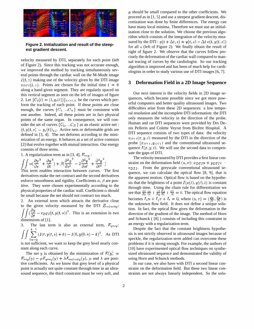
Figure 2. Initialization and result of the steep-est gradient descent.

velocity measured by DTI, separately for each point (leftof Figure 2). Since this tracking was not accurate enough,we improved the method by tracking simultaneously sev-eral points through the cardiac wall on the M-Mode image� ������

making use of the velocity given by the DTI image��� � � ������ . Points are chosen for the initial time� ���

along a hand given segment. They are regularly spaced onthis vertical segment as seen on the left of images of figure2. Let � � 9 ��� � ���� 9 ���� � "���9 ��� be the curves which per-form the tracking of each point. If these points are closeenough, the curves � � " = = = � � must be consistent withone another. Indeed, all these points are in fact physicalpoints of the same organ. In consequence, we will con-sider the set of curves � � " = = = � � as an elastic active net :�����'������ ����� ���� � ���� : . Active nets or deformable grids aredefined in [3, 4]. The net deforms according to the mini-mization of an energy. It behaves as a set of active contours[2] that evolve together with mutual interaction. Our energyconsists of three terms.1. A regularization term as in [3, 4],

��� -50 :� ��� ��� �� � ( ) � �� � ( )�� ��� (�

� � ( ( )! � ( �� � � ( ) � ( �� � ( (

This term enables interaction between curves. The firstderivatives make the net contract and the second derivativesenforce smoothness and rigidity. Coefficients

�, � are pos-

itive. They were chosen experimentally according to thephysical properties of the cardiac wall. Coefficient

�should

be small because the net should not contract too much.2. An external term which attracts the derivative closeto the given velocity measured by the DTI

� 23-5476�8�97:<; :� � ��� �� �#" ��� � � ������'���$� � ( . This is an extension in two

dimensions of [1].3. The last term is also an external term,

� 0 � -5; :� �&%(' ()%('+* (

� ������'����� )!, " ���-� �'�-� $� )., ( . As DTI

is not sufficient, we want to keep the grey level nearly con-stant along each curve.

The net�

is obtained by the minimization of���-�� ��/� -/0 �-�� )10 � 0 � -/; � �� )32 � 23-5476�8�97:<; � �� , 0 and 2 are posi-

tive coefficients. As we know that grey level of a physicalpoint is actually not quite constant through time in an ultra-sound sequence, the third constraint must be very soft, and

0 should be small compared to the other coefficients. Weproceed as in [1, 5] and use a steepest gradient descent, dis-cretization was done by finite differences. The energy canhave many local minima. Therefore we must use an initial-ization close to the solution. We choose the previous algo-rithm which consists of the integration of the velocity mea-sured by the DTI :

�'��� )54 ���� 768�������� )54 � � �����'������ � for all

�(left of Figure 2). We finally obtain the result of

right of figure 2. We observe that the curves follow pre-cisely the deformation of the cardiac wall compared to man-ual tracing of curves by the cardiologist. So our trackingalgorithm is improved and has been of much help for cardi-ologists in order to study various use of DTI images [6, 7].

3 Deformation Field in a 2D Image Sequence

Our next interest is the velocity fields in 2D image se-quences, which became possible since we got more pow-erful computers and better quality ultrasound images. Twodifficulties arise from these 2D sequences: a low tempo-ral resolution and the incomplete DTI information: the DTIonly measures the velocity in the direction of the probe.Human and rat DTI sequences were provided by Drs De-nis Pellerin and Colette Veyrat from Bicetre Hospital. ADTI sequence consists of two types of data: the velocity��� � � �-9 ��'��� measured by the DTI in the direction of theprobe

�-9 � � � �� � � � and the conventional ultrasound se-quence

��� 9���'>�� . We will use the second data to compen-

sate the gaps of DTI.The velocity measured by DTI provides a first linear con-

straint on the deformation field� :� � : 9 � � � : ) � � � � � �� � � � . From the greyscale conventional ultrasound se-

quence, we can calculate the optical flow [8, 9], that isthe apparent motion. Optical flow is based on the hypothe-sis that the brightness of a point

� �-9 ���� >��'���� >>�� is constant

through time. Using the chain rule for differentiation wesee that ; �;�< ;�<; : ) ; �; ; ; ;; : ) ; �; : �=� . The optical flow equation

becomes� < : ) � ; � ) � : ���

, where�-:� � � � ;�<; : ; ;; : is

the unknown flow field. It does not define a unique solu-tion. In fact, the optical flow gives the deformation in thedirection of the gradient of the image. The method of Hornand Schunck ( [8] ) consists of including this constraint inan energy with a regularization term.

Despite the fact that the constant brightness hypothe-sis is not strictly observed in ultrasound images because ofspeckle, the regularization term added can overcome theseproblems if it is strong enough. For example, the authors of[10] have experimented optical flow techniques on synthe-sized ultrasound sequence and demonstrated the validity ofusing Horn and Schunck methods.

In our case, we also have with DTI a second linear con-straint on the deformation field. But these two linear con-straints are not always linearly independent. So the solu-

2

tion cannot be the resolution of the system. Since more-over ultrasound images are very noisy, we propose a so-lution inspired by Horn and Schunck method. The field� :�� 9 �'>�� > � �-9 ����� � we are looking for will satisfy, whenpossible, the optical flow constraint, the agreement with theDTI velocity and a first order regularity constraint. We in-clude these three constraints in an energy minimization. Foreach frame

�:� � :� � ���� ��� � � 9 � � � : ) � � � � � " � � � � (

) � � � < : ) � ; � ) � : ( )5� ����� :�� ( ) ��� � � ( �=where � is the image domain. Coefficients

�and � are

positive and are chosen experimentally. We minimize thisenergy with a steepest gradient descent.

Figure 3. Velocity field with our method.

Figure 4. Improvement provided by DTI. Opti-cal Flow without and with DTI

An example of result is given in Figure 3. The resultsare satisfying compared with simple optical flow as shownin figure 4. Direction is modified and we get a more reg-ular field without increasing the diffusion. But some prob-lems due to the acquisition persist. First, gaps in the lateral

wall imply gaps in optical flow for which DTI cannot al-ways compensate since it is always in the direction of theprobe. Second, the image of lateral walls consists of hor-izontal spots because the transmitted signal is oblique tothem, and so the gradient of the image is not really whatexpected, and so is optical flow. However, the deformationfield is quite accurate and regular around the anterior andposterior walls.

In order to fill gaps, we adapt the ideas developped in[9] and include a temporal regularization. This asssumptionof temporal regularity is relevant since the temporal resolu-tion is high enough to provide small displacement betweensuccessive images. The minimized energy is then :��� :� � �� � � � � � ���

� 9 � � � : ) � � � � � " ��� � � () � �� < : ) � ; � ) � : ( )�� ��� � :�� ( ) � � � � ( >=

Here�

is a ��� gradient. It ensures interaction between dif-ferent frames. An example of result is shown in figure 5.As in [9], the result is much more coherent. We can see thatmissing information is completed by the neighbouring im-ages. The velocity field is much more regular and completearound the myocardium wall than the first one.

Figure 5. Velocity field with a spatio-temporalregularization.

If the displacement field is still not satisfying, we haveto use a fast algorithm to improve ultrasound images by en-hancing edges. We chose the “sticks algorithm” introducedby [11] to reduce speckle noise and improve the edge infor-mation as shown in figure 6. We must carefully select the

3

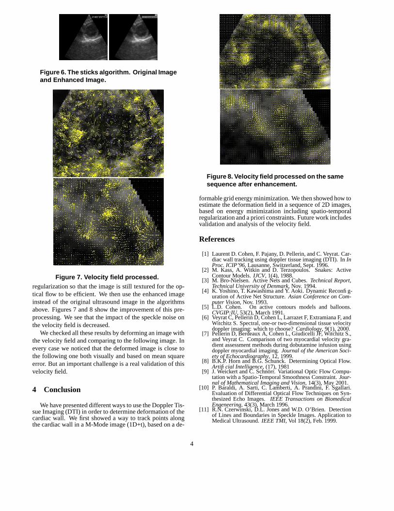
Figure 6. The sticks algorithm. Original Imageand Enhanced Image.

Figure 7. Velocity field processed.regularization so that the image is still textured for the op-tical flow to be efficient. We then use the enhanced imageinstead of the original ultrasound image in the algorithmsabove. Figures 7 and 8 show the improvement of this pre-processing. We see that the impact of the speckle noise onthe velocity field is decreased.

We checked all these results by deforming an image withthe velocity field and comparing to the following image. Inevery case we noticed that the deformed image is close tothe following one both visually and based on mean squareerror. But an important challenge is a real validation of thisvelocity field.

4 Conclusion

We have presented different ways to use the Doppler Tis-sue Imaging (DTI) in order to determine deformation of thecardiac wall. We first showed a way to track points alongthe cardiac wall in a M-Mode image (1D+t), based on a de-

Figure 8. Velocity field processed on the samesequence after enhancement.

formable grid energy minimization. We then showed how toestimate the deformation field in a sequence of 2D images,based on energy minimization including spatio-temporalregularization and a priori constraints. Future work includesvalidation and analysis of the velocity field.

References

[1] Laurent D. Cohen, F. Pajany, D. Pellerin, and C. Veyrat. Car-diac wall tracking using doppler tissue imaging (DTI). In InProc. ICIP’96, Lausanne, Switzerland, Sept. 1996.

[2] M. Kass, A. Witkin and D. Terzopoulos. Snakes: ActiveContour Models. IJCV, 1(4), 1988.

[3] M. Bro-Nielsen. Active Nets and Cubes. Technical Report,Technical University of Denmark, Nov. 1994.

[4] K. Yoshino, T. Kawashima and Y. Aoki. Dynamic Reconfig-uration of Active Net Structure. Asian Conference on Com-puter Vision, Nov. 1993.

[5] L.D. Cohen. On active contours models and balloons.CVGIP:IU, 53(2), March 1991.

[6] Veyrat C, Pellerin D, Cohen L, Larrazet F, Extramiana F, andWitchitz S. Spectral, one-or two-dimensional tissue velocitydoppler imaging: which to choose? Cardiology, 9(1), 2000.

[7] Pellerin D, Berdeaux A, Cohen L, Giudicelli JF, Witchitz S.,and Veyrat C. Comparison of two myocardial velocity gra-dient assessment methods during dobutamine infusion usingdoppler myocardial imaging. Journal of the American Soci-ety of Echocardiography, 12, 1999.

[8] B.K.P. Horn and B.G. Schunck. Determining Optical Flow.Artificial Intelligence, (17), 1981

[9] J. Weickert and C. Schnorr. Variational Optic Flow Compu-tation with a Spatio-Temporal Smoothness Constraint. Jour-nal of Mathematical Imaging and Vision, 14(3), May 2001.

[10] P. Baraldi, A. Sarti, C. Lamberti, A. Prandini, F. Sgallari.Evaluation of Differential Optical Flow Techniques on Syn-thesized Echo Images. IEEE Transactions on BiomedicalEngeneering, 43(3), March 1996.

[11] R.N. Czerwinski, D.L. Jones and W.D. O’Brien. Detectionof Lines and Boundaries in Speckle Images. Application toMedical Ultrasound. IEEE TMI, Vol 18(2), Feb. 1999.

4