estimation of coefficients for modelling ships from sea
TRANSCRIPT
Estimation of Coefficients for Modelling Ships from
Sea Trials Using Stepwise Optimization Methods and
Considering Trim and Draught Conditions
Dissertation
zur
Erlangung des akademischen Grades
Doktor-Ingenieur (Dr.-Ing.)
der Fakultät für Maschinenbau und Schiffstechnik
der Universität Rostock
vorgelegt von
M.Sc. Dae Won Kim
geb. am 05.01.1983 in Daegu, Südkorea
Rostock, 2019

Gutachter:
Prof. Dr.-Ing. habil. Mathias Paschen, Universität Rostock, Lehrstuhl für Meerestechnik
Prof. Dr.-Ing. habil. Knud Benedict, Hochschule Wismar, Institut ISSIMS
Prof. Dr.-Ing. habil. Nikolai Kornev, Universität Rostock, Lehrstuhl für Modellierung
und Simulation
Tag der Einreichung: 25.09.2018
Tag der Verteidigung:03.06.2019

I
I. Selbstä ndigkeitserklä rung
Hiermit wird bestätigt, dass die vorliegende Arbeit selbständig verfasst und keine anderen
als angegeben Quellen und Hilfsmittel benutzt sowie Zitate und gedankliche Ü bernahmen
kenntlich gemacht wurden.
Rostock, den 25.09.2018
Ort/Datum Unterschrift

II
II. List of contents
1. Introduction .................................................................................................. 1
2. State of the art in ship manoeuvrability ..................................................... 4
2.1 Prediction of ship manoeuvrability ................................................................. 4
2.1.1 Coordinate systems ......................................................................................... 4
2.1.2 Equations of a ship’s manoeuvring motion .................................................... 5
2.1.3 Representation of hydrodynamic force and moment ...................................... 7
2.1.4 Determination of the hydrodynamic coefficients ......................................... 10
2.2 Manoeuvring characteristics and corresponding tests .................................. 16
2.3 Influence of trim and draught on ship manoeuvrability ............................... 23
3. Fundamentals of mathematical optimization ........................................... 38
3.1 Introduction................................................................................................... 38
3.2 Unconstrained optimization .......................................................................... 39
3.2.1 Quasi-Newton Algorithm ............................................................................. 40
3.2.2 Derivative-free optimization ......................................................................... 42
3.3 Constrained optimization .............................................................................. 46
3.3.1 Interior point method .................................................................................... 47
3.3.2 Sequential quadratic programming method .................................................. 49
4. Coefficients estimation using mathematical optimization ...................... 54
4.1 Introduction................................................................................................... 54
4.2 About the mathematical optimization ........................................................... 54
4.3 Setting of optimization problems.................................................................. 55

III
4.4 Sea trial measurements and corrections for reference data .......................... 59
4.5 Optimization results ...................................................................................... 65
4.6 Conclusion .................................................................................................... 76
5. Coefficients estimation for various trim and draught conditions .......... 78
5.1 Introduction................................................................................................... 78
5.2 Optimization problems ................................................................................. 78
5.3 Validation of optimization results using other sea trial data ........................ 81
5.4 Estimation of hydrodynamic coefficients considering various trim and
draught conditions ........................................................................................ 91
5.5 Conclusion .................................................................................................... 96
6. Conclusion ................................................................................................... 98
7. References .................................................................................................. 100
Appendix A. Details of manoeuvres for chapter 5 .............................................. 105

IV
III. List of figures
Figure 2.1 Coordinate systems .......................................................................................... 5
Figure 2.2 Methods of manoeuvring prediction .............................................................. 10
Figure 2.3 Effort/Cost versus accuracy of manoeuvring prediction methods ................. 11
Figure 2.4 System identification for estimating hydrodynamic coefficients by Abkowitz ... 14
Figure 2.5 System identification for estimating hydrodynamic coefficients by Rhee et al. .. 15
Figure 2.6 Inherent dynamic stability .............................................................................. 17
Figure 2.7 Course-keeping ability ................................................................................... 17
Figure 2.8 Trajectory of the ship during turning ............................................................. 20
Figure 2.9 Time histories of rudder angle and heading during zig-zag test .................... 21
Figure 2.10 Trajectory of the ship during stopping test .................................................. 21
Figure 2.11 Yaw rate to rudder angle curve from spiral tests ......................................... 22
Figure 2.12 Time histories of the turning rate from pull-out test .................................... 22
Figure 2.13 User interface for hull coefficients in SIMOPT ........................................... 25
Figure 2.14 Comparison of trajectories for turning manoeuvre with 35 degrees of rudder
angle according to changes of mean draught ................................................ 26
Figure 2.15 Comparison of trajectories for zig-zag manoeuvre with 10 degrees of rudder
angle according to changes of mean draught ................................................ 28
Figure 2.16 Comparison of heading changes for zig-zag manoeuvre with 10 degrees of
rudder angle according to changes of mean draught .................................... 29
Figure 2.17 Comparison of trajectories for zig-zag manoeuvre with 20 degrees of rudder
angle according to changes of mean draught ................................................ 29
Figure 2.18 Comparison of heading changes for zig-zag manoeuvre with 20 degrees of
rudder angle according to changes of mean draught .................................... 30
Figure 2.19 Comparison of trajectories for turning manoeuvre with 35 degrees of rudder
angle according to changes of trim ............................................................... 31
Figure 2.20 Comparison of trajectories for zig-zag manoeuvre with 10 degrees of rudder
angle according to changes of trim ............................................................... 32

V
Figure 2.21 Comparison of heading changes for zig-zag manoeuvre with 10 degrees of
rudder angle according to changes of trim ................................................... 33
Figure 2.22 Comparison of trajectories for zig-zag manoeuvre with 20 degrees of rudder
angle according to changes of trim ............................................................... 33
Figure 2.23 Comparison of heading changes for zig-zag manoeuvre with 20 degrees of
rudder angle according to changes of trim ................................................... 34
Figure 2.24 Manoeuvre results with various trim conditions .......................................... 35
Figure 2.25 Concepts of pivot point ................................................................................ 36
Figure 3.1 Concept of the mathematical optimization .................................................... 38
Figure 3.2 Simplexes for 𝑛 = 2 (left) and 𝑛 = 3 (right) ................................................. 44
Figure 3.3 Concept operation for the Nelder-Mead algorithm ........................................ 44
Figure 4.1 Concept of optimization process to estimate hydrodynamic coefficients ...... 55
Figure 4.2 Results of sensitivity analysis on hydrodynamic coefficients........................ 58
Figure 4.3 Means of data acquisition: S-VDR and ECDIS ............................................. 62
Figure 4.4 Comparisons of measurement data and corrected data .................................. 64
Figure 4.5 Comparison of optimization algorithms: straight motion .............................. 68
Figure 4.6 Comparison of optimization algorithms: zig-zag manoeuvre ........................ 69
Figure 4.7 Comparison of optimization algorithms: turning manoeuvre ........................ 69
Figure 4.8 Comparison of trajectories: straight motion ................................................... 70
Figure 4.9 Comparison of trajectories: zig-zag motion ................................................... 71
Figure 4.10 Comparison of heading change: zig-zag manoeuvre ................................... 71
Figure 4.11 Comparison of trajectories: turning manoeuvre ........................................... 72
Figure 4.12 Comparison of heading change for optimization steps 2 and 3: Interior point
algorithm with constraint .............................................................................. 73
Figure 4.13 Comparison of heading change for optimization steps 2 and 3: Interior point
algorithm without constraint ......................................................................... 73
Figure 4.14 Comparison of heading change for optimization steps 2 and 3: Nelder-Mead
algorithm ....................................................................................................... 74

VI
Figure 4.15 History of iteration: straight motion ............................................................. 75
Figure 4.16 History of iteration: zig-zag manoeuvre ...................................................... 75
Figure 4.17 History of iterations: turning manoeuvre ..................................................... 76
Figure 5.1 Comparison of heading change between sea trial data 2 and simulation results .. 83
Figure 5.2 Comparison of trajectories between sea trial data 2 and simulation results .. 83
Figure 5.3 Comparison of heading change between sea trial data 3 and simulation results .. 84
Figure 5.4 Comparison of trajectories between sea trial data 3 and simulation results .. 84
Figure 5.5 Comparison of heading change between sea trial data 4 and simulation results .. 85
Figure 5.6 Comparison of trajectories between sea trial data 4 and simulation results .. 85
Figure 5.7 Comparison of heading change between sea trial data 1 and various simulations 89
Figure 5.8 Comparison of trajectories between sea trial data 1 and various simulations 90
Figure 5.9 Comparison of heading change between sea trial data 5 and various simulations 90
Figure 5.10 Comparison of trajectories between sea trial data 5 and various simulations .... 91
Figure 5.11 Results of curve fitting for 𝑋𝑢𝑢 and 𝑋𝑢4 .................................................... 94
Figure 5.12 Comparison of heading change for the simulation results of Clarke estimation
and suggested formula .................................................................................. 96

VII
IV. List of tables
Table 2.1 Characteristics for methods of manoeuvrability prediction ............................ 13
Table 2.2 Recommended manoeuvring tests by various organisations ........................... 19
Table 2.3 Influence of draught changes on turning manoeuvre ...................................... 26
Table 2.4 Influence of draught changes on zig-zag manoeuvre with 10 degrees of rudder
angle .............................................................................................................. 27
Table 2.5 Influence of draught changes on zig-zag manoeuvre with 20 degrees of rudder
angle .............................................................................................................. 28
Table 2.6 Influence of trim changes on turning manoeuvre ............................................ 30
Table 2.7 Influence of trim changes on zig-zag manoeuvre with 10 degrees of rudder
angle .............................................................................................................. 31
Table 2.8 Influence of trim changes on zig-zag manoeuvre with 20 degrees of rudder
angle .............................................................................................................. 32
Table 4.1 Results of sensitivity analysis on hydrodynamic coefficients ......................... 57
Table 4.2 Variables on each optimization step ................................................................ 59
Table 4.3 Details of the reference vessel for comparing optimization algorithms .......... 59
Table 4.4 Summary of conditions for sea trials ............................................................... 60
Table 4.5 Time history for zig-zag manoeuvre ............................................................... 61
Table 4.6 Time history for turning manoeuvre................................................................ 61
Table 4.7 Detailed conditions of optimization ................................................................ 65
Table 4.8 Summarization of Clarke coefficients and optimized coefficients.................. 66
Table 4.9 Manoeuvre characteristics of reference data and simulation results ............... 67
Table 5.1 Details of the reference vessel ......................................................................... 78
Table 5.2 Summary of conditions for sea trials ............................................................... 79
Table 5.3 Variables on each optimization step ................................................................ 79
Table 5.4 Detailed conditions of optimization ................................................................ 80
Table 5.5 Summarization of Clarke coefficients and optimized coefficients.................. 81

VIII
Table 5.6 Manoeuvre characteristics for reference data and simulation results .............. 82
Table 5.7 Comparison of optimized coefficients for two sea trial data which have the same
trim and draught condition (Case of the data 1 and 2) ................................. 86
Table 5.8 Comparison of optimized coefficients for two sea trial data which have the same
trim and draught condition (Case of the data 4 and 5) ................................. 87
Table 5.9 Comparison of manoeuvre characteristics for simulation results and sea trial
data (Case of the data 1 and 2)...................................................................... 88
Table 5.10 Comparison of manoeuvre characteristics for simulation results and sea trial
data (Case of the data 4 and 5)...................................................................... 89
Table 5.11 Correction values for estimation formulae which are based on three sea trial
measurements ............................................................................................... 93
Table 5.12 Environmental conditions for the sea trial for validation of the estimation
formulae ........................................................................................................ 94
Table 5.13 Comparison of coefficients between Clarke estimation and suggested formulas
...................................................................................................................... 95
Table 5.14 Comparison of manoeuvre characteristics for the simulation results of Clarke
estimation and suggested formula ................................................................ 96

IX
V. List of abbreviations
ANS Advanced Nautical Simulator
BFGS Broyden-Fletcher-Goldfarb-Shanno algorithm
CFD Computational Fluid Dynamics
DFP Davidon-Fletcher-Powell formula
DWT Deadweight Tonnage
EFK Extended Kalman Filter
G/T Gross Tonnage
IMO International Maritime Organization
ISTTES (Project name) Integrative Simulationsanwendung unter Beachtung von
Trimm- und Tiefgangänderungen zur effektiven Schiffssteuerung und
Verbesserung der Handlungssicherheit in Gefahrensituationen
ITTC International Towing Tank Conference
KKT Karush-Kuhn-Tucker conditions
LCF Longitudinal Centre of Flotation
LPP Length Between Perpendiculars
MMG Mathematical Modelling Group
NMEA Nautical Marine Electronics Association
RANS Reynolds-averaged Navier-Stokes equations
SHS Ship Handling Simulator
SQP Sequential Quadratic Programming
VDR Voyage Data Recorder

1
1. Introduction
The development of overall science has been accompanied with the progress of computer
technology since the middle of the 20th century. Advanced mathematical model on ship’s
behaviour can explain complex physical phenomena more easily, and the computer tech-
nology can introduce various derivative ideas.
This can have a great influence on both a construction and a navigation of a ship. From
the ship’s design to its actual operation, various forms of application of information pro-
cessing technology are no longer surprising matters. The improvement of the computer
performance can be seen in the estimation of ship’s manoeuvrability, more precisely the
estimation of hydrodynamic coefficients acting on ship’s hull. In the initial ship design
stage, it is possible to precheck the ship’s manoeuvrability and seaworthiness, and to re-
flect them in the actual ship construction. This can lead to positive effects such as reliable
ship, cost reduction and process innovation.
In 2006, the international towing tank conference (ITTC) provided state-of-art for pre-
dicting the manoeuvring behaviour of ships. Most of the methods except for the database
method and the free model test are system based manoeuvring simulation or computa-
tional fluid dynamics (CFD) based estimation methods. All above methods estimate the
ship’s hydrodynamic coefficients based on the ship’s equations of motion, and these can
be utilized to estimate ship’s manoeuvrability. Among these, the most popular methods
used in the early design stage are the captive model test and CFD based manoeuvring
simulation. The above methods are enabling to conduct experiments without using a full-
scale sized model, and it is possible to estimate hydrodynamic coefficients and corre-
sponding manoeuvrability of proper reliability.
However, this ship manoeuvrability estimation can be applied differently for existing
ships. The system based manoeuvring simulation for the estimation of ship manoeuvra-
bility is applied to various purposes in conjunction with the computer development men-
tioned above. Simulation based ship handling training has made great progress in the ed-
ucation and training of seafarers. A sailing decision support program, which uses simula-
tions and network technologies, collects data from various navigation equipment to ena-
ble safer and more effective ship operation. Unmanned or autonomous vessels, which are
currently under active research, reflect this trend well.

2
Estimation of the ship’s hydrodynamic coefficients can also be done through full-scale
sea trial. This is the only way to estimate the hydrodynamic coefficients without addi-
tional tests such as model tests and CFD. This can be done through a mathematical pro-
cedure called system identification. This mathematical process conducts optimization for
the hydrodynamic coefficients to represent ship’s manoeuvrability in a mathematical way.
Abkowitz, Oltmann and Hess conducted representative studies related to this, and the
follow-up studies are still carried out at present.
Normally, estimation of hydrodynamic coefficients is conducted according to the specific
loading conditions of the ship. In other words, ship’s manoeuvrability and its correspond-
ing coefficients can be considered to one specific trim and draught condition of the ship
at the time. However, in practice, ships operate with various trim and draught conditions.
In some cases, situations may arise where all trim and draught conditions need to be con-
sidered, depending on the purpose of the simulation.
Therefore, this thesis proposes a method for estimation of the hydrodynamic coefficients
using full-scale sea trial and a method of system identification. Also, based on this, a
proposal for a new estimation method that can consider various trim and draught condi-
tions will be given here. The new estimation method will be in the form of suggesting an
additional calibration formula that can complement the existing empirical estimation for-
mulas for the hydrodynamic coefficients involving different trim and draught parameters.
This makes it possible to estimate a simpler and more efficient estimation of the hydro-
dynamic coefficients from sea trials.
This thesis is composed as follows. Chapter 2 describes the theoretical background for
estimating ship manoeuvrability. The ship's coordinate system, equations of motion, hy-
drodynamic coefficients acting on the hull, and influence of trim and draught on ship’s
manoeuvrability are included.
Chapter 3 introduces the mathematical optimization, which is a method for estimating the
hydrodynamic coefficients acting on the hull for this thesis. After introducing the basic
concepts of the mathematical optimization, an introduction to the representative algo-
rithms of constrained and unconstrained optimization is described in this chapter.

3
Chapter 4 applies the algorithms introduced in Chapter 3 to actual sea trial data and the
optimization results are compared and verified. Details of the sea trial vessel, trial proce-
dures and comparison of optimization results are discussed in this chapter.
Chapter 5 conducts the mathematical optimization with an interior point algorithm, which
is finally chosen from the algorithm comparison in Chapter 4. Five sea trial data with
three different trim and draught conditions are used for the optimization. Based on the
optimization result, the trim and draft correction coefficients are calculated and a correc-
tion formula for the final coefficient estimation is suggested.
Chapter 6 describes the final summary and future work based on the previous contents.

4
2. State of the art in ship manoeuvrability
In this chapter concepts, following definitions and corresponding literature study are dis-
cussed:
• Coordinate systems
• Equations of motions
• Hydrodynamic coefficients
• Manoeuvring characteristics and trials
• Influence of trim and draught
2.1 Prediction of ship manoeuvrability
A ship simulation has been developed with an improvement of computer processing tech-
nology. It has become possible to more effectively and simply estimate the manoeuvra-
bility of the ship during its initial design stage. Even in the case of existing vessels, the
simulation can be used for various purposes such as training and navigation decision sup-
port. Ship modelling in a mathematical way, especially for estimating hydrodynamic co-
efficients acting on the hull, is one of the most important processes to realize this.
2.1.1 Coordinate systems
Two right-handed three degrees of freedom coordinate systems, the earth-fixed coordi-
nate 𝑂0 − 𝑥0𝑦𝑜𝑧0 and the ship-fixed coordinate 𝑂 − 𝑥𝑦𝑧 are selected to estimate ship’s
manoeuvrability. Both the 𝑂0 − 𝑥0𝑦𝑜 and the 𝑂 − 𝑥𝑦 horizontal planes placed on the un-
disturbed free surface and velocities for heave, rolling and pitching are ignored. Figure
2.1 shows an overview of the coordinate systems. Vertical axes 𝑧0 and 𝑧 are directed
downwards:

5
Figure 2.1 Coordinate systems
where 𝛹 is a heading angle, 𝛽 is a drift angle, 𝛿 is a rudder angle, �⃗� is ship’s speed and
𝑟 is yaw rate, respectively. Heading can be determined by an angle between 𝑥0 and 𝑥 axes.
A ship’s position in each moment is determined by the ship’s centre of gravity in the
earth-fixed coordinate system. The drift angle is determined by an angle between a direc-
tion of speed �⃗� and the 𝑥 axis. The ship’s speed �⃗� is expressed by a combination of axial
speeds 𝑢 and 𝑣. The axial speeds can be calculated as follows:
1 𝑢 = |�⃗� | cos 𝛽
𝑣 = −|�⃗� | sin 𝛽.
(1)
2.1.2 Equations of a ship’s manoeuvring motion
Equations of a ship’s motion are based on the Newton’s second law. In the inertial coor-
dinate, the earth-fixed coordinate, the equations can be defined as follows [1]:
2 𝑋0 = 𝑚�̈�0𝐺
𝑌0 = 𝑚�̈�0𝐺
𝑁0 = 𝐼𝑧𝐺�̈�,
(2)
where
𝑋0, 𝑌0: component of external force acting on 𝑥0 and 𝑦0 axis, respectively,

6
𝑁0: component of external moment for 𝑧 axis,
𝑚: mass of a ship,
�̈�0𝐺 , �̈�0𝐺: component of acceleration acting on 𝑥0 and 𝑦0 axis, respectively,
𝐼𝑧𝐺: moment of inertia of a ship about the z axis and
�̈�: yaw acceleration.
Equation (2), which is focused on the earth-fixed coordinates, can be converted into equa-
tions in the body-fixed coordinates. External forces acting on 𝑥 and 𝑦 axes are the fol-
lowing:
3 𝑋 = 𝑋0 𝑐𝑜𝑠 𝛹 + 𝑌0 𝑠𝑖𝑛 𝛹
𝑌 = −𝑋0 𝑠𝑖𝑛 𝛹 + 𝑌0 𝑐𝑜𝑠 𝛹.
(3)
The right side of Equation (3) can be transformed to terms of kinetic parameters for the
ship-fixed coordinate by applying relations between kinematic parameters for both coor-
dinates. Components of speed in the earth-fixed coordinate are expressed by a ship’s lon-
gitudinal and lateral speed components, 𝑢𝐺 and 𝑣𝐺 , and heading 𝛹:
4 𝑥0̇ = 𝑢𝑔 𝑐𝑜𝑠 𝛹 − 𝑣𝑔 𝑠𝑖𝑛 𝛹
𝑦0̇ = 𝑢𝑔 𝑠𝑖𝑛 𝛹 + 𝑣𝑔 𝑐𝑜𝑠 𝛹.
(4)
Components of acceleration in the earth-fixed coordinate can be provided by differenti-
ating Equation (4):
5 �̈�0 = �̇�𝑔 𝑐𝑜𝑠 𝛹 − �̇�𝑔�̇� 𝑠𝑖𝑛 𝛹 − �̇�𝑔 𝑠𝑖𝑛 𝛹 − �̇�𝑔�̇� 𝑐𝑜𝑠 𝛹
�̈�0 = �̇�𝑔 𝑠𝑖𝑛 𝛹 + �̇�𝑔�̇� 𝑐𝑜𝑠 𝛹 + �̇�𝑔 𝑐𝑜𝑠 𝛹 − �̇�𝑔�̇� 𝑠𝑖𝑛 𝛹.
(5)
Equation (3) can be converted into the equations in the body-fixed coordinate by substi-
tuting Equations (2) and (5):
6 𝑋 = 𝑚(�̇�𝑔 − 𝑣𝑔�̇�)
𝑌 = 𝑚(�̇�𝑔 + 𝑢𝑔�̇�).
(6)
7
Considering a ship is symmetrical based on a hydrodynamic centre, it is more convenient
to place the ship-fixed coordinate on the midship point than the ship’s centre of gravity.
Then, the ship’s new longitudinal and lateral speed components are as follows:
7 𝑢𝑔 = 𝑢
𝑣𝑔 = 𝑣 + 𝑥𝑔�̇�.
(7)
The equations of motion in the body-fixed coordinate, placed on the midship point, are
as follows.
8 𝑋 = 𝑚(�̇� − 𝑣�̇� − 𝑥𝑔�̇�2)
𝑌 = 𝑚(�̇� + 𝑢�̇� + 𝑥𝑔�̈�)
(8)
The external moment acting on the 𝑧 axis and moment of inertia in the ship-fixed coordi-
nate can be modified from the moment acting on the earth-fixed coordinate and the lon-
gitudinal centre of gravity position.
9 𝑁 = 𝑁0 + 𝑌𝑥𝑔 and 𝐼𝑧 = 𝐼𝑧𝐺 + 𝑚𝑥𝐺
2
then, 𝑁 = 𝐼𝑧�̈� + 𝑚𝑥𝑔(�̇� + 𝑢𝑟)
(9)
The first-order differential for the heading can be converted into the yaw rate 𝑟. The equa-
tions of motion in the ship-fixed coordinate, lying on the ship’s midship point, can be
finally provided as follows.
10 𝑋 = 𝑚(�̇� − 𝑣𝑟 − 𝑥𝑔𝑟2)
𝑌 = 𝑚(�̇� + 𝑢𝑟 + 𝑥𝑔�̇�)
𝑁 = 𝐼𝑧�̇� + 𝑚𝑥𝑔(�̇� + 𝑢𝑟)
(10)
2.1.3 Representation of hydrodynamic force and moment
Various studies on expression of hydrodynamic force and moment have been carried out
by many researchers. These can be classified into two kinds: a polynomial model and a
modular model.
Model by Abkowitz Abkowitz presented polynomials for the hydrodynamic force and
moment, which is based on the Tayler series. He premises that forces can be determined
by instantaneous values of kinematic parameters, without unsteady effects [2]. This
8
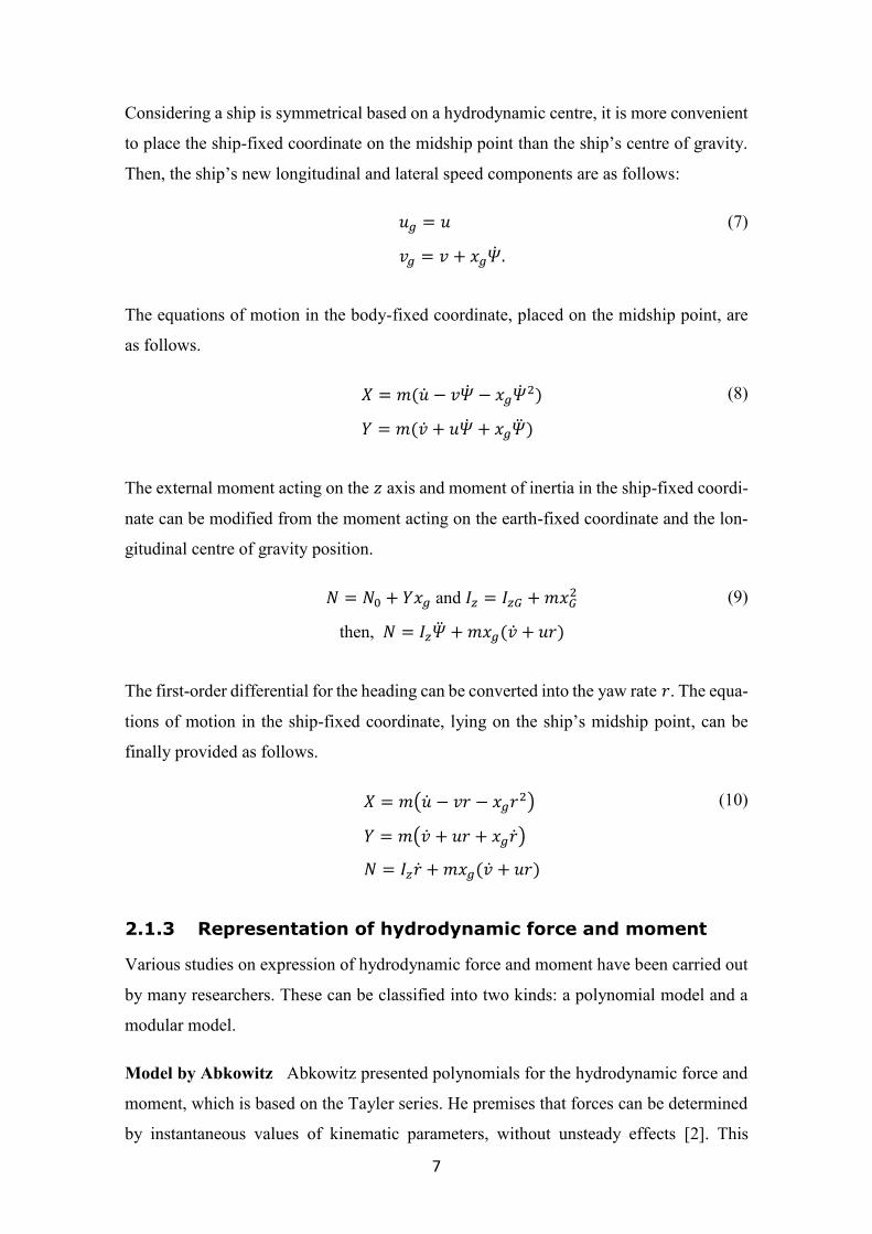
means that the unsteady influences can be ignored when a time step for hydrodynamic
changes is extremely smaller than the one for the ship’s motion. The polynomials are
functions of the kinematic parameters and rudder angle:
11 𝑋, 𝑌 𝑎𝑛𝑑 𝑁 = 𝑓(𝑢, 𝑣, 𝑟, �̇�, �̇�, �̇�, 𝛿). (11)
Abkowitz suggested polynomials based on a third-order Taylor series, as follows [3]:
12 𝑋 = 𝑋0 +𝜕𝑋
𝜕�̇��̇� +
𝜕𝑋
𝜕𝑢∆𝑢 +
1
2
𝜕2𝑋
𝜕𝑢2(∆𝑢)2 +
1
2
𝜕2𝑋
𝜕𝑣2𝑣2 +
1
2
𝜕2𝑋
𝜕𝑟2𝑟2 +
1
2
𝜕2𝑋
𝜕𝛿2𝛿2
+1
2
𝜕2𝑋
𝜕𝑣𝑟𝑣𝑟 +
1
2
𝜕2𝑋
𝜕𝑣𝛿𝑣𝛿 +
1
2
𝜕2𝑋
𝜕𝑟𝛿𝑟𝛿 +
1
6
𝜕3𝑋
𝜕𝑢3(∆𝑢)3 +
1
6
𝜕3𝑋
𝜕𝑣2𝑢𝑣2∆𝑢
+1
6
𝜕3𝑋
𝜕𝑟2𝑢𝑟2∆𝑢 +
1
6
𝜕3𝑋
𝜕𝛿2𝑢𝛿2∆𝑢 +
1
6
𝜕3𝑋
𝜕𝑣𝑟𝑢𝑣𝑟∆𝑢 +
1
6
𝜕3𝑋
𝜕𝑣𝛿𝑢𝑣𝛿∆𝑢
+1
6
𝜕3𝑋
𝜕𝑟𝛿𝑢𝑟𝛿∆𝑢
(12)
13 𝑌 = 𝑌0 +𝜕𝑌
𝜕�̇��̇� +
𝜕𝑌
𝜕�̇��̇� +
𝜕𝑌
𝜕𝑢∆𝑢 +
𝜕𝑌
𝜕𝑣𝑣 +
𝜕𝑌
𝜕𝑟𝑟 +
𝜕𝑌
𝜕𝛿𝛿 +
1
2
𝜕2𝑌
𝜕𝑢2(∆𝑢)2
+1
2
𝜕2𝑌
𝜕𝑣𝑢𝑣∆𝑢 +
1
2
𝜕2𝑌
𝜕𝑟𝑢𝑟∆𝑢 +
1
2
𝜕2𝑌
𝜕𝛿𝑢𝛿∆𝑢 +
1
6
𝜕3𝑌
𝜕𝑣3𝑣3 +
1
6
𝜕3𝑌
𝜕𝑟3𝑟3
+1
6
𝜕3𝑌
𝜕𝛿3𝛿3 +
1
6
𝜕3𝑌
𝜕𝑣𝑢2𝑣(∆𝑢)2 +
1
6
𝜕3𝑌
𝜕𝑣𝑟2𝑣𝑟2 +
1
6
𝜕3𝑌
𝜕𝑣𝛿2𝑣𝛿2
+1
6
𝜕3𝑌
𝜕𝑟𝑢2𝑟(∆𝑢)2 +
1
6
𝜕3𝑌
𝜕𝑟𝑣2𝑟𝑣2 +
1
6
𝜕3𝑌
𝜕𝑟𝛿2𝑟𝛿2 +
1
6
𝜕3𝑌
𝜕𝛿𝑢2𝛿(∆𝑢)2
+1
6
𝜕3𝑌
𝜕𝛿𝑣2𝛿𝑣2 +
1
6
𝜕3𝑌
𝜕𝛿𝑟2𝛿𝑟2 +
1
6
𝜕3𝑌
𝜕𝑣𝑟𝛿𝑣𝑟𝛿
(13)
14 𝑁 = 𝑁0 +𝜕𝑁
𝜕�̇��̇� +
𝜕𝑁
𝜕�̇��̇� +
𝜕𝑁
𝜕𝑢∆𝑢 +
𝜕𝑁
𝜕𝑣𝑣 +
𝜕𝑁
𝜕𝑟𝑟 +
𝜕𝑁
𝜕𝛿𝛿 +
1
2
𝜕2𝑁
𝜕𝑢2(∆𝑢)2
+1
2
𝜕2𝑁
𝜕𝑣𝑢𝑣∆𝑢 +
1
2
𝜕2𝑁
𝜕𝑟𝑢𝑟∆𝑢 +
1
2
𝜕2𝑁
𝜕𝛿𝑢𝛿∆𝑢 +
1
6
𝜕3𝑁
𝜕𝑣3𝑣3 +
1
6
𝜕3𝑁
𝜕𝑟3𝑟3
+1
6
𝜕3𝑁
𝜕𝛿3𝛿3 +
1
6
𝜕3𝑁
𝜕𝑣𝑢2𝑣(∆𝑢)2 +
1
6
𝜕3𝑁
𝜕𝑣𝑟2𝑣𝑟2 +
1
6
𝜕3𝑁
𝜕𝑣𝛿2𝑣𝛿2
+1
6
𝜕3𝑁
𝜕𝑟𝑢2𝑟(∆𝑢)2 +
1
6
𝜕3𝑁
𝜕𝑟𝑣2𝑟𝑣2 +
1
6
𝜕3𝑁
𝜕𝑟𝛿2𝑟𝛿2 +
1
6
𝜕3𝑁
𝜕𝛿𝑢2𝛿(∆𝑢)2
+1
6
𝜕3𝑁
𝜕𝛿𝑣2𝛿𝑣2 +
1
6
𝜕3𝑁
𝜕𝛿𝑟2𝛿𝑟2 +
1
6
𝜕3𝑁
𝜕𝑣𝑟𝛿𝑣𝑟𝛿,
(14)

9
where 𝑋0, 𝑌0 and 𝑁0 are derivatives for the initial steady state, where longitudinal speed
only exists. Derivatives in Equations (12) to (14) can be shorten as follows:
15 𝜕𝑋
𝜕𝑢= 𝑋𝑢,
𝜕3𝑌
𝜕𝑣𝑟2= 𝑌𝑣𝑟𝑟 ,
𝜕3𝑁
𝜕𝑣𝑟𝛿= 𝑁𝑣𝑟𝛿 , ⋯
(15)
Model by Norrbin Norrbin provided a mathematical model, which is a transitional
model between a polynomial and a modular model [4]. The model includes functions for
speed components for three axes, a thrust 𝑇, a propeller torque 𝑄 and an inflow velocity
to the rudder 𝑐. A wake and thrust deduction factors are independent from the propeller
loading. Norrbin’s equations are as follows [5]:
16 𝑇 = 𝑇(𝑢, 𝑛)
𝑄 = 𝑄(𝑢, 𝑛)
𝑐 = 𝑐(𝑢, 𝑛)
𝑋 = 𝑋�̇��̇� + 𝑋𝑢𝑢𝑢2 + 𝑋𝑣𝑟𝑣𝑟 + 𝑋𝑣𝑣𝑣2
+𝑋𝑐|𝑐|𝛿𝛿𝑐|𝑐|𝛿2 + 𝑋𝑐|𝑐|𝛽𝛿𝑐|𝑐|𝛽𝛿 + (1 − 𝑡)𝑇
𝑌 = 𝑌�̇��̇� + 𝑌𝑢𝑟𝑢𝑟 + 𝑌𝑢𝑣𝑢𝑣 + 𝑌𝑣|𝑣|𝑣|𝑣| + 𝑌𝑐|𝑐|𝛿2𝑐|𝑐|𝛿2
+𝑌𝑐|𝑐||𝛽||𝛿|𝑐|𝑐||𝛽||𝛿| + 𝑌𝑇𝑇
𝑁 = 𝑁�̇��̇� + 𝑁𝑢𝑟𝑢𝑟 + 𝑁𝑢𝑣𝑢𝑟 + 𝑁|𝑣|𝑟|𝑣|r + 𝑁𝑐|𝑐|𝛿𝑐|𝑐|𝛿
+𝑁𝑐|𝑐||𝛽||𝛽||𝛿|𝑐|𝑐||𝛽||𝛽||𝛿| + 𝑁𝑇𝑇
T = 𝑇𝑢𝑢𝑢2 + 𝑇𝑢𝑛𝑢𝑛 + 𝑇𝑛|𝑛|𝑛|𝑛|
(𝐼𝑃 − 𝑄𝑛)�̇� = 𝑄𝐹 + 𝑄𝑢𝑢𝑢2 + 𝑄𝑢𝑛𝑢𝑛 + 𝑄𝑛|𝑛|𝑛|𝑛| + 𝑄𝑛𝑛 + 𝑄𝜇𝜇
c = 𝑐𝑢𝑛𝑢𝑛 + 𝑐𝑛𝑛𝑛2 , 𝑛 > 0
c = 0 , n < 0
(16)
where, 𝜇 is an engine output ratio. Considering lateral and rotational direction for the
symmetrical hull, a form of the absolute value, |𝑎|, is applied.
MMG modular model A research group focused on the ‘standardization of a mathe-
matical model for ship manoeuvring predictions’ was created by the Japan Society of
Naval Architects and Ocean Engineers, and this group provided the current Manoeuvring
Modelling Group (MMG) model [6]. Each hydrodynamic force or moment has three

10
modules, which are acting on the ship hull, the propeller and the rudder, respectively.
Each component concerns both individual and interacting effects.
17 𝑋 = 𝑋𝐻 + 𝑋𝑃 + 𝑋𝑅
𝑌 = 𝑌𝐻 + 𝑌𝑃 + 𝑌𝑅
𝑁 = 𝑁𝐻 + 𝑁𝑃 + 𝑁𝑅
(17)
2.1.4 Determination of the hydrodynamic coefficients
ITTC summarized the state-of-the-art of the ship’s manoeuvring prediction methods. Fig-
ure 2.2 shows an overview of methods for manoeuvring predictions and Figure 2.3 shows
an overview of accuracy against cost. Methods can be categorized into three features: a
prediction without simulation, with system based manoeuvring simulation and CFD
based manoeuvring simulation.
Figure 2.2 Methods of manoeuvring prediction [7]

11
Figure 2.3 Effort/Cost versus accuracy of manoeuvring prediction methods [7]
The full-scale trial is an intuitive way to figure out manoeuvrability of an object. Nomoto
estimated indices of K and T, which are steering coefficients for rudder effect and ship’s
reaction inertia, from the analysis of full-scale zig-zag trials, using linear equation of mo-
tion [8,9]. Inoue et al. conducted sea trials with various types of vessels and those
manoeuvring results were compared to numerical simulation results [10]. The most fa-
mous trial is conducted by the 278,000 DWT tanker ESSO Osaka in confined waters by
Crane [11]. He showed an impact of the bottom clearance on ship’s manoeuvrability and
his approach greatly influenced the methods and procedures for sea trial to estimate ma-
noeuvrability. However, this method is not possible to control environmental effects thor-
oughly and is hard for merchant vessels due to economic reasons.
The model tests are an alternative way to complement deficiencies of the full-scale trial.
Forces and kinetic parameters are measured during the trials and there the hydrodynamic
coefficients can be derived for certain mathematical model of a vessel. In a model basin,
which includes a towing tank and a cavitation tunnel and others, scaled models are tested
and resultant forces and corresponding parameters can be measured. A set of model tests
can also be applied into empirical regression and corresponding formulas. Norrbin, Inoue
et al., Clarke et al., Kijima et al. and Kose proposed foundations of empirical formulas

12
for the hydrodynamic coefficients of the equations of motion and subsequent researches
are still continuing [5,10,12–14].
CFD techniques can provide insight into the ship with the application of computational
calculation. Since 1960s, after Hess and Smith introduced three-dimensional CFD model
in aviation, CFD has shown outstanding progress with the advancement of computing
technology [15]. Compared to the conventional model tests, this method can react to lots
of models and external conditions easily. CFD for the shipbuilding industry was intro-
duced later than the aviation, because of the existence of free surface and complex ship
geometry [16].
In spite developing a numerical calculation, conventional model tests are still the main
source to examine manoeuvring force and moment. As shown in Figure 2.3, the conven-
tional model tests are the best solutions to satisfy both accuracy and cost without bias to
either side, when a designated ship is at the early design stage or under construction. On
the other hand, the methods above are relatively more expensive than the system identi-
fication method.
Table 2.1 summarizes characteristics for the predictions methods by ITTC [7]. This study
applies a system identification method, which optimizes the hydrodynamic coefficients
in a way of mathematical optimization. The optimization procedure requires a set of ref-
erences and initial conditions. These are delivered from real ship sea trials and existing
empirical estimation formulas, which are based on the idea of Norrbin and Clarke [5,12].
The system identification has developed with the progress of computational calculation.
Abkowitz used the extended Kalman filter (EKF) to estimate hydrodynamic coefficients
for the ESSO Osaka [17]. The resultant coefficients and an effective simulation showed
that results of the numerical simulation were fitted to motions during the sea trials.

13
Table 2.1 Characteristics for methods of manoeuvrability prediction
Method Concept Advantage Disadvantage
Free model test
- Perform pre-defined ma-
noeuvres, such as zig-zag
or turning manoeuvres
- Model ship’s actuators are
controlled by autopilots
- Close to reality
- Test results are delivered
in real time
- Relatively low cost
- Possibility for control of
environmental conditions in
a basin
- Require relatively large
test area
- Impossible to deliver
physical insight
- Impossible to connect to
mathematical models
- Environmental effects
also should be considered a
scale effect
Captive model test
- Carried out in a tow tank,
with planar motion mecha-
nism and rotating arm de-
vice
- Hydrodynamic coeffi-
cients can be obtained from
analysing test results
- Perfect control of environ-
mental effects during tests
- Created mathematical
model can also be utilized
for bridge simulators
- Desired result can be de-
livered after post-pro-
cessing of test results
- Quality of the mathemati-
cal model is dependent on
the size of test matrix
- Test should be carried out
by skilled personnel to re-
duce re-test, which needs a
lot of time
Empirical method
- Estimate hydrodynamic
coefficients based on multi-
ple previous tests
- Test results are utilized in
the fast-time and real-time
simulators
- Short processing time
- Relatively low cost
- Easy to change certain pa-
rameters of a ship
- The accuracy and reliabil-
ity are quite low
- Sensitive to the shallow
water effect
- Consideration of hull
form detail is missing
System identification
- Estimate hydrodynamic
coefficients by mathemati-
cal optimization
- Utilize sea trial measure-
ments into parameter iden-
tification directly
-Apply to generate addi-
tional manoeuvres based on
results of free model tests
- Applicable for both
model-scale and full-scale
manoeuvres
- Resultant coefficients are
not physically correct
- Acquired raw data might
have noise and this can in-
terfere to a process
Viscous flow CFD
- RANS calculation takes a
role of the captive model
test
- Physical model is not re-
quired
- CFD gives physical in-
sight
- Applicable for both
model-scale and full-scale
tests
- Much experience is re-
quired for stable test results
- A large amount of exper-
tise and coding is required
Potential flow CFD
- CFD methods, which does
not apply RANS calcula-
tion
- Require less effort than
the RANS method
- Reliability is lower than
the RANS method

14
(a) Concept of the coefficients identification
(b) Heading simulation of zig-zag manoeuvre20°/20° after the identification
Figure 2.4 System identification for estimating hydrodynamic coefficients by Abkowitz [17]
Rhee et al. also used the EKF with the ESSO Osaka, but this research used the MMG
model for the numerical simulations [18]. They implemented an importance of sensitivity
for each manoeuvre and conducted coefficients identification according to the result of
the sensitivity analysis. Simulations results using estimated coefficients showed satisfac-
tory trajectory and other kinematic parameters compared to the sea trial results.
Zhang and Zou applied ε-support vector regression to the coefficients identification [19].
The mathematical model of Abkowitz was applied to the identification process and re-
sultant coefficients were verified by the PMM test results.

15
(a) Estimation procedure
(b) Trajectory of zig-zag manoeuvre20°/20° after the identification
Figure 2.5 System identification for estimating hydrodynamic coefficients by Rhee et al. [18]
Tran et al. introduced SQP and BFGS algorithms to obtain optimization results [20]. Co-
efficients identification was conducted after sensitivity analysis for each manoeuvre and
their simulation results were compared with the sea trial data.

16
Many of previous studies on the system identification were conducted using ESSO Osaka
as a reference data and the EKF. It is assumed that these are caused by difficulty of ob-
taining sufficient sea trial data for estimating hydrodynamic coefficients and limitations
of the optimization algorithm at that time. In addition, as mentioned in Table 2.1, it is
considered that there has been less research than other methods of manoeuvrability esti-
mation because of the problem of having physical uncertainty about the estimated coef-
ficients.
This study was carried out considering the advantages and disadvantages of the system
identification, mentioned above. As a preparation of this thesis, Kim introduced a math-
ematical optimization process using a simulation result based on Azimuth propulsion
ferry ship as a reference [21]. Based on this result, Kim et al. conducted a mathematical
optimization by applying sea trial data as a reference, and simulation results using tuned
coefficients are closer to the reference compared with simulation results using a basic
coefficients estimation of the corresponding simulator [22]. In this study, optimization
was performed based on the mathematical models and corresponding hydrodynamic co-
efficients of Norrbin and Clarke. Reference data required for optimization process were
obtained by sea trial.
2.2 Manoeuvring characteristics and corresponding tests
Ship manoeuvrability is an ability of a ship, which presents keeping and altering its state
of motion with certain controls. This includes straight motions with constant speed or
increasing speed and changing course manually. IMO provided standards for ship
manoeuvring characteristics to evaluate qualities of the manoeuvrability [23].
Inherent dynamic stability A ship is dynamically stable on a straight course if it can
fix a new straight course after a disturbance without any steering actions by a helmsman.
Figure 2.6 shows a concept of the inherent dynamic stability. An unstable ship moves
continuously into an irrational course in contrast with a stable ship, which can reset its
course after an interruption. The consequent deviation from the original heading relies on
the extend of inherent stability and on the weight and length of the disturbance.

17
Figure 2.6 Inherent dynamic stability
Course-keeping ability The course-keeping ability is a means of a steered ship, which
keeps a straight path toward a prearranged course without inordinate oscillations of rudder
or heading. As shown in Figure 2.7, a ship with inherent dynamic stability can only keep
its original course with certain control action. However, a ship with an inherent dynamic
instability can also maintain its original course if it applies a frequent control action.
Figure 2.7 Course-keeping ability
Initial turning / course-changing ability The initial turning ability is described by the
change-of-heading response to a control action. A ship which has good initial turning
ability can alter to its original course. This can be expressed by the ‘P number’, which
represents the rate of heading change as to the helm angle [24]. Norrbin defines this index
as follows:
18 𝑃 =𝜓′(𝑡′ = 1)
𝛿′(𝑡′ = 1),
(18)
where 𝜓′, 𝛿′ and 𝑡′ are the nondimensionalised heading, rudder angle and time, respec-
tively [9]. Norrbin studied the P number for different ships and proposed the value P=0.3
as a lower limit for proper manoeuvrability of a ship [25].

18
Yaw checking ability The yaw checking ability is a ship performance measurement of
how fast a turning motion defeats and settles a course [26]. It can be measured from the
response to counter-rudder in a certain state of turning manoeuvre. The overshoot angle
or time to yaw-check of course change test and zig-zag test can examine the yaw checking
ability.
Turning ability The turning ability is an ability to turn a ship with a hard-over rudder.
Corresponding results are an advance, a tactical diameter and a transfer. Details are dis-
cussed later.
Stopping ability The stopping ability is measured from ‘track reach’ and ‘time to dead
in water’ by a stop engine-full astern manoeuvre after a steady motion with full engine
speed. Normally a ship deviates due to environmental disturbances and initial test condi-
tions.
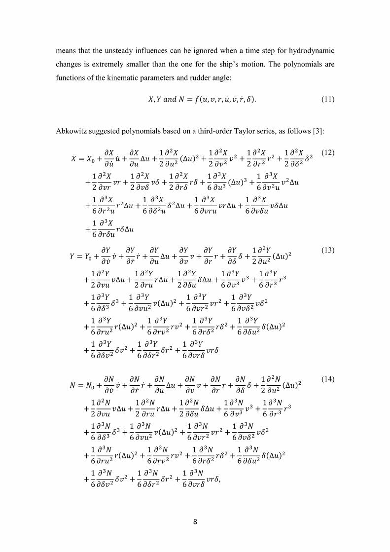
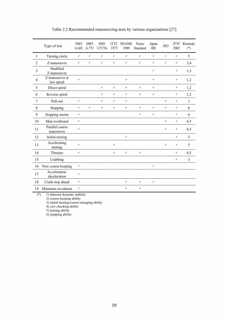
As shown in Table 2.2, ITTC summarized a total of 19 manoeuvring tests, which are
recommended by various organisations. 15 of these provide information on manoeuvring
characteristics, which are mentioned above [27].
The standard of IMO resolution MSC.137(76) is chosen for this dissertation. Test details
and their satisfactory criteria are as follows [28].
Turning test A turning test evaluates a ship’s turning ability. It performs to both star-
board and port with a 35-degree rudder angle or designed maximum angle at the test speed.
Command for rudder execution comes after the ship is at a steady state with zero yaw
rate. Figure 2.8 shows a concept and kinematic parameters of the turning test. The stand-
ard requires that the advance should not be more than 4.5 ship lengths and the tactical
diameter should be more than 5 ship lengths in the manoeuvre.
19
Table 2.2 Recommended manoeuvring tests by various organisations [27]
Type of test IMO
A.601
IMO
A.751
IMO
137(76)
ITTC
1975
SNAME
1989
Norse
Standard
Japan
RR ISO
ITTC
2002
Remarks
(*)
1 Turning circle ✓ ✓ ✓ ✓ ✓ ✓ ✓ ✓ ✓ 5
2 Z-manoeuvre ✓ ✓ ✓ ✓ ✓ ✓ ✓ ✓ ✓ 3,4
3 Modified
Z-manoeuvre ✓ ✓ 1,3
4 Z-manoeuvre at
low speed ✓ ✓ ✓ ✓ 1,2
5 Direct spiral ✓ ✓ ✓ ✓ ✓ ✓ 1,2
6 Reverse spiral ✓ ✓ ✓ ✓ ✓ ✓ 1,2
7 Pull-out ✓ ✓ ✓ ✓ ✓ ✓ 1
8 Stopping ✓ ✓ ✓ ✓ ✓ ✓ ✓ ✓ ✓ 6
9 Stopping inertia ✓ ✓ ✓ ✓ 6
10 Man-overboard ✓ ✓ ✓ 4,5
11 Parallel course
manoeuvre ✓ ✓ ✓ 4,5
12 Initial turning ✓ ✓ 3
13 Accelerating
turning ✓ ✓ ✓ ✓ 5
14 Thruster ✓ ✓ ✓ ✓ ✓ 4,5
15 Crabbing ✓ 3
16 New course keeping ✓ ✓
17 Acceleration/
deceleration ✓
18 Crash stop ahead ✓ ✓ ✓ ✓
19 Minimum revolution ✓ ✓ ✓
(*) 1) inherent dynamic stability
2) course-keeping ability
3) initial turning/course-changing ability
4) yaw checking ability
5) turning ability
6) stopping ability

20
Figure 2.8 Trajectory of the ship during turning [1]
Zig-zag test A zig-zag test evaluates the ship’s initial turning, the yaw checking and the
course-keeping abilities. It begins by executing a certain amount of rudder angle from an
initial straight manoeuvre, called ‘first execute’. When a specified deviation from the
ship’s original heading occurs, the rudder angle is altered to the opposite side, called ‘sec-
ond execute’. Normally two kinds of zig-zag tests, 10°/10° and 20°/20° tests are applied.
Each test has 10° and 20° of heading deviation, respectively. Figure 2.9 shows character-
istic parameters and time histories for the rudder angle and heading during the test. Over-
shoot angles and initial turning time to second execute are chosen as manoeuvrability
parameters. For the initial turning ability, with the 10°/10° test, the ship should not travel
more than 2.5 ship lengths by the time for 10° of heading deviation. For the yaw checking
and course-keeping ability, satisfactory criteria is as follows:
- The first overshoot angle for the 10°/10° test should not exceed
10° if L/V is less than 10s;
20° if L/V is 30s or more; and
(5+1/2(L/V)) ° if L/V is 10s more, but less than 30s.
- The second overshoot angle for the 10°/10° test should not exceed
25° if L/V is less than 10s;
40° if L/V is 30s or more; and

21
(17.5+0.75(L/V)) ° if L/V is 10s or more, but less than 30s.
- The first overshoot angle for the 20°/20° test should not exceed 25°.
Figure 2.9 Time histories of rudder angle and heading during zig-zag test [1]
Stopping test A stopping test evaluates the stopping ability. A full astern stopping test
is conducted to measure the track reach of a ship from the moment of full-astern order to
the place ship is stopped. Figure 2.10 shows a concept of the test. The standard requires
that the track reach should not exceed 15 to 20 ship lengths, considering a ship’s displace-
ment.
Figure 2.10 Trajectory of the ship during stopping test [1]
Spiral test A spiral test is included as additional manoeuvres in the standard of IMO. It
evaluates the inherent dynamic stability and the course-keeping ability. A direct spiral
test conducts a series of turning manoeuvres. Rudder commands for the turning change
every 5 degrees from 15 degrees of one side to 0 degrees. This is repeated for both the
port and starboard side. Each turning manoeuvre should be recorded at least one minute
tinit t1-3

22
after the yaw rate remains constant. A reverse spiral test can substitute the direct spiral
test to define an instability loop. In the test, a ship is steered to obtain a constant yaw rate
and the mean rudder angle is required to measure the yaw rate. Then the yaw rate versus
rudder angle can be plotted on the area of the instability. Figure 2.11(a) and Figure 2.11(b)
show results of spiral tests for a stable ship and instable ship, respectively.
Figure 2.11 Yaw rate to rudder angle curve from spiral tests [1]
Pull-out test A pull-out test evaluates a ship’s dynamic stability on a straight course.
After the completion of the turning manoeuvre, the rudder is set to midship position, and
from there a steady yaw rate is obtained. If the ship is stable, the rate of turn decreases to
zero. The continuing rates of turn indicates the degree of instability at the 0° of the rudder
angle. Figure 2.12(a) and Figure 2.12(b) compare results of the pull-out tests for a stable
and an unstable ship.
Figure 2.12 Time histories of the turning rate from pull-out test [1]

23
2.3 Influence of trim and draught on ship manoeuvrability
Since IMO adopted a guideline, “Interim Guidelines for Estimating Manoeuvring Perfor-
mance in Ship Design”, in 1985, many studies about estimation and evaluation of the
manoeuvrability have been provided and this enhanced accuracy of prediction at the de-
sign stage. While the guideline gives a criterion only for ship’s full loaded even keel
condition, most of sea trials are carried out in ballast conditions for practical reasons.
Changes of trim and draught have a remarkable effect on a ship’s manoeuvrability due to
the change of multiple corresponding ship’s conditions, such as displacement, a location
of the centre-of-pressure for the sway force, rudder inflow angle and so on. It is easily
shown that a ship with a trim by stern is common when the ship is in ballast condition
due to its relatively stable manoeuvrability than other trim and draught conditions.
Most studies on manoeuvrability regarding loading conditions are focusing on the corre-
sponding changes of displacement, stern shape and rudder area. Kijima et al. and Kose
studied an influence and an importance of trim and draught conditions on a ship’s ma-
noeuvrability. In order to estimate a ship’s manoeuvrability in different trim and draught
conditions, they conducted captive model tests with various types of ships and four trim
and draught conditions: fully loaded, half loaded, ballast with even keel and ballast aft
trim conditions [13,14,29]. The prediction results based on the estimation agreed well
with the measured results of free running model tests. Yasukawa et al. investigated an
influence of the load condition on the effect of rudder force [30]. Inoue et al. suggested a
set of empirical formulae from model experiments considering both in even keel and
trimmed conditions using the aspect ratio 𝑘 as follows [31]:
19 𝑌′𝛽 = (
1
2𝜋 𝑘 + 𝑓 (𝐶𝐵
𝐵
𝐿)) (1.0 +
2𝑡
3𝑑𝑚)
𝑌′𝑟 =
1
4𝜋 𝑘 (1.0 +
0.80𝑡
𝑑𝑚)
𝑁′𝛽 = 𝑘 (1.0 −
0.27𝑡
𝑙𝛽𝑑𝑚)
𝑁′𝑟 = (0.54𝑘 − 𝑘2) (1.0 +
0.30𝑡
𝑑𝑚)
where, 𝑙𝛽 = 𝑘/ (1
2𝜋 𝑘 + 𝑓 (𝐶𝐵
𝐵
𝐿))
(19)

24
Influence of ship manoeuvrability due to changes in draught and trim can be confirmed
using fast time simulator. For this experiment, a fast time simulator SIMOPT of ISSIMS
GmbH and a G/T 6686t model ship were used for the simulations. Details of the model
ship will be referred in Chapter 4. A ship’s dynamic capabilities of the SIMOPT are based
on the mathematical models of Norrbin and Clarke [5,12] which is in between the poly-
nomial model and modular model. Clarke’s formulae are reduced from the same form of
Inoue et al. [31]. Figure 2.13 presents an example of user interface for SIMOPT. Hull
forces and moment of the equations consist of the following components:
20 𝑋ℎ = 𝑋𝑢𝑝(�̇� − �̇�𝑔) + 𝑋𝑣𝑟𝑣𝑟 + 𝑋𝑢𝑢𝑢|𝑢| + 𝑋𝑢4𝑢3|𝑢|
+𝑋𝑢𝑣𝑣𝑣𝑢|𝑣|𝑣2 + 𝑓(𝑢𝑡ℎ𝑟𝑒𝑠ℎ𝑜𝑙𝑑)
𝑌ℎ = 𝑌𝑣𝑝(�̇� − �̇�𝑔) + 𝑌𝑟𝑝�̇� + 𝑌𝑢𝑟𝑢𝑟 + 𝑌𝑢𝑣|𝑢|𝑣 + 𝑌𝑛𝑜𝑛𝑙𝑖𝑛𝑒𝑎𝑟
𝑁ℎ = 𝑁𝑟𝑝(�̇� − �̇�𝑔) + 𝑁𝑟𝑣�̇� + 𝑁𝑢𝑟|𝑢|𝑟 + 𝑁𝑢𝑣𝑢𝑣 + 𝑁𝑛𝑜𝑛𝑙𝑖𝑛𝑒𝑎𝑟,
(20)
where 𝑢, 𝑣, 𝑟 are speed components through water, and �̇�, �̇�, �̇� and �̇�𝑔, �̇�𝑔, �̇�𝑔 are acceler-
ation components through water and over ground, respectively. The term 𝑓(𝑢𝑡ℎ𝑟𝑒𝑠ℎ𝑜𝑙𝑑)
is only active when a pre-defined threshold velocity is greater than a ship’s velocity. Sets
of nonlinear coefficients 𝑌𝑛𝑜𝑛𝑙𝑖𝑛𝑒𝑎𝑟 and 𝑁𝑛𝑜𝑛𝑙𝑖𝑛𝑒𝑎𝑟 can be composed by the following co-
efficients:
𝑌𝑛𝑜𝑛𝑙𝑖𝑛𝑒𝑎𝑟 = [𝑌𝑟𝑟, 𝑌𝑣𝑣, 𝑌𝑣𝑟 , 𝑌𝑣𝑟𝑡, 𝑌𝑣𝑣𝑣𝑟 , 𝑌𝑟𝑟𝑡, 𝑌𝑣𝑣𝑡, 𝑌4𝑣2𝑟𝑡, 𝑌𝑛𝑜𝑛_𝑡𝑢𝑟𝑛𝑖𝑛𝑔_𝑝𝑜𝑖𝑛𝑡]
𝑁𝑛𝑜𝑛𝑙𝑖𝑛𝑒𝑎𝑟 = [𝑁𝑣𝑟 , 𝑁𝑟𝑟𝑡, 𝑁𝑣𝑣𝑡, 𝑁𝑟𝑟 , 𝑁𝑣𝑣, 𝑁𝑣4𝑟2, 𝑁𝑣𝑟𝑡, 𝑁5𝑣3𝑟𝑡, 𝑁𝑛𝑜𝑛_𝑡𝑢𝑟𝑛𝑖𝑛𝑔_𝑝𝑜𝑖𝑛𝑡].

25
Figure 2.13 User interface for hull coefficients in SIMOPT
The coefficients, 𝑌𝑛𝑜𝑛_𝑡𝑢𝑟𝑛𝑖𝑛𝑔_𝑝𝑜𝑖𝑛𝑡 and 𝑁𝑛𝑜𝑛_𝑡𝑢𝑟𝑛𝑖𝑛𝑔_𝑝𝑜𝑖𝑛𝑡 can vary according to a turn-
ing point. The standard estimation for the SIMOPT system, named ‘Clarke estimation’,
uses the following ship parameters:
- Length
- Breadth
- Draught, fore
- Draught, aft
- Displacement
- Block coefficient
- Nominal power
- Nominal speed
The experimental method is as follows. In comparing the manoeuvrability according to
the draught change, trim is fixed to the even keel condition. On the contrary, simulations
for the comparison of the manoeuvrability with the change of the trim are carried out by
changing only the trim at the same mean draught. The mean draughts were set in five
conditions, ranging from 3.9m to 5.9m with every 0.5m. The trims are total of 5 condi-
tions, from -2m to +2m per meter. Because the sign of the trim differs from related or-
ganizations and industries, this thesis uses the trim by stern as positive and trim by head
as minus based on the document of IMO [28].
𝑇𝑟𝑖𝑚 = 𝐷𝑟𝑎𝑢𝑔ℎ𝑡𝑎𝑓𝑡 − 𝐷𝑟𝑎𝑢𝑔ℎ𝑡𝑓𝑜𝑟𝑤𝑎𝑟𝑑

26
Table 2.3 shows simulation results of the turning manoeuvre with the change of the
draught. Advance, tactical diameter and kinematic parameters were selected for manoeu-
vre characteristics to be compared. Turning manoeuvre results show that as the draught
increases, the advance and the tactical diameter also increases. This leads to increased
distance of straight motion before turning and larger turning radius. Tendencies of dis-
tance parameters relate also to corresponding kinematic parameters. Figure 2.14 shows
comparison for trajectories, based on the corresponding simulation results.
Table 2.3 Influence of draught changes on turning manoeuvre
Mean draught
[m]
TC35P
Advance
[m]
Tactical di-
ameter [m]
Final speed
[kts]
Final ROT
[deg/min]
Final drift
angle [deg]
3.9 304.43 157.54 7.42 -75.849 13.77
4.4 316.8 167.19 7.12 -71.896 13.21
4.9 328.33 177.14 6.83 -68.527 12.75
5.4 338.18 182 6.61 -66.055 12.36
5.9 347.51 186.63 6.33 -63.552 12.09
Remark ROT: Rate of Turn
Figure 2.14 Comparison of trajectories for turning manoeuvre with 35 degrees of rudder angle
according to changes of mean draught

27
Table 2.4 and Table 2.5 show influence of draught change for zig-zag manoeuvre with
10 degrees and 20 degrees of rudder angle, respectively. First and second overshoot an-
gles, dimensionless parameters and elapsed time for certain amount of heading change
were selected for the characteristics to be compares. Definitions for manoeuvre charac-
teristics are as follows:
- Initial turning parameter: dimensionless distance between starting point and
the first point (xinit in Figure 2.9) where ship’s heading meets rudder command,
in relation to ship’s length;
- Turning & checking parameter: dimensionless period of time (x1-3 in Figure
2.9) between first and third zero crossing of heading, in relation to ship speed
performance (L/V);
- Initial response time: initial time of ship’s heading response to rudder com-
mand.
Comparison shows that the overshoot angles increase consistently as the draught in-
creases. Although the first overshoot at 5.9m for zig-zag with 10 degrees does not follow
the trend with others, the rest parameters at that draught maintain a steady trend. This is
considered to be due to the increase of ship’s displacement and resistance, which is caused
by the increase of the underwater portion of the hull. Figure 2.15 to Figure 2.18 show
comparison for trajectories and heading changes, based on the corresponding simulation
results.
Table 2.4 Influence of draught changes on zig-zag manoeuvre with 10 degrees of rudder angle
Mean draught
[m]
ZZ10S
First
overshoot
[deg]
Second
overshoot
[deg]
Initial
turning
parameter
Turning &
checking
parameter
Initial
response
time [s]
3.9 3.3 3.1 1.38 7.35 16
4.4 3.4 4.1 1.47 8.04 17
4.9 3.7 4.1 1.56 8.47 18
5.4 3.9 5.1 1.64 9.16 19
5.9 3.4 5.2 1.73 9.5 20

28
Table 2.5 Influence of draught changes on zig-zag manoeuvre with 20 degrees of rudder angle
Mean draught
[m]
ZZ20S
First
overshoot
[deg]
Second
overshoot
[deg]
Initial
turning
parameter
Turning &
checking
parameter
Initial
response
time [s]
3.9 8.4 7.2 1.64 9.6 19
4.4 8.8 8.1 1.73 10.2 20
4.9 9.2 9.1 1.81 10.89 21
5.4 9.6 8.8 1.9 11.4 22
5.9 10.2 9.8 1.99 12.09 23
Figure 2.15 Comparison of trajectories for zig-zag manoeuvre with 10 degrees of rudder angle
according to changes of mean draught

29
Figure 2.16 Comparison of heading changes for zig-zag manoeuvre with 10 degrees of rudder
angle according to changes of mean draught
Figure 2.17 Comparison of trajectories for zig-zag manoeuvre with 20 degrees of rudder angle
according to changes of mean draught

30
Figure 2.18 Comparison of heading changes for zig-zag manoeuvre with 20 degrees of rudder
angle according to changes of mean draught
Table 2.6 and Figure 2.19 show the changes of manoeuvre characteristics for turning ma-
noeuvre according to the trim changes. As the trim changes from ‘by the head’ to ‘by the
stern’, the turning circle increases and the corresponding kinetic parameters are also con-
sistent.
Table 2.6 Influence of trim changes on turning manoeuvre
Trim
[m]
TC35P
Advance
[m]
Tactical di-
ameter [m]
Final speed
[kts]
Final ROT
[deg/min]
Final drift
angle [deg]
-2 289.96 116.12 4.26 -67.194 18.72
-1 317.2 150.43 5.19 -65.444 15.12
0 347.51 186.63 6.33 -63.552 12.09
+1 381.95 229.03 7.55 -61.037 9.73
+2 419.91 277.72 8.72 -57.975 7.94
Remark ROT: Rate of Turn

31
Figure 2.19 Comparison of trajectories for turning manoeuvre with 35 degrees of rudder angle
according to changes of trim
Table 2.7 and Table 2.8 show changes in the zig-zag manoeuvre as the trim changes. The
characteristics to be compared are the same as those of the previous draught change. As
the trim changes from 'by the head' to 'by the stern', the initial turning ability decreases
but the yaw checking ability becomes better. Figure 2.20 to Figure 2.23 show comparison
for trajectories and heading changes, based on the corresponding simulation results.
Table 2.7 Influence of trim changes on zig-zag manoeuvre with 10 degrees of rudder angle
Trim
[m]
ZZ10S
First
overshoot
[deg]
Second
overshoot
[deg]
Initial
turning
parameter
Turning &
checking
parameter
Initial
response
time [s]
-2 8.1 17.2 1.55 12.09 18
-1 5.2 9.3 1.64 10.36 19
0 3.4 5.2 1.73 9.5 20
+1 2.7 3.3 1.81 9.41 21
+2 2.1 2.8 1.9 9.67 22

32
Table 2.8 Influence of trim changes on zig-zag manoeuvre with 20 degrees of rudder angle
Trim
[m]
ZZ20S
First
overshoot
[deg]
Second
overshoot
[deg]
Initial
turning
parameter
Turning &
checking
parameter
Initial
response
time [s]
-2 19.1 21.2 1.81 14.08 21
-1 13 13.6 1.9 12.52 22
0 10.2 9.8 1.99 12.09 23
+1 6.8 7.1 2.16 11.75 25
+2 6 7.3 2.25 12.26 26
Figure 2.20 Comparison of trajectories for zig-zag manoeuvre with 10 degrees of rudder angle
according to changes of trim

33
Figure 2.21 Comparison of heading changes for zig-zag manoeuvre with 10 degrees of rudder
angle according to changes of trim
Figure 2.22 Comparison of trajectories for zig-zag manoeuvre with 20 degrees of rudder angle
according to changes of trim

34
Figure 2.23 Comparison of heading changes for zig-zag manoeuvre with 20 degrees of rudder
angle according to changes of trim
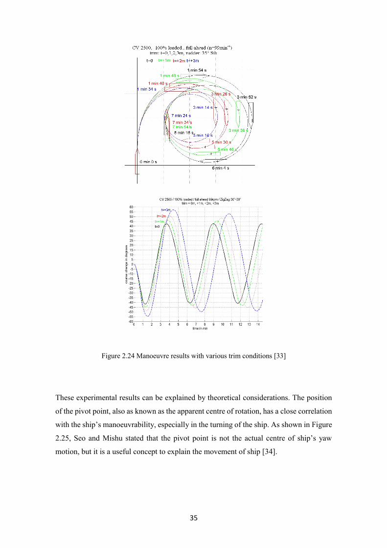
Krüger introduced comparison for a ship’s manoeuvrability with various trim condition
by Benedict [32,33]. He found that a change of trim is subject to major changes of a ship’s
manoeuvrability, but this influence is not subject to the linear laws. Figure 2.24 shows
simulation results for a turning manoeuvre and a zig-zag manoeuvre for a fully loaded
2,500 TEU container ship. All manoeuvres are conducted under the same mean draught,
and trim is the only control variable for the comparison. Trim conditions are provided
every 1 metre from the even keel condition to 3 metres by the head. Results confirm that
increased trim by the head affects to greater overshoot angle and to decrease turning circle.
These are consistent with the effect of trim changes, shown in the Table 2.6 to Table 2.8.
35
Figure 2.24 Manoeuvre results with various trim conditions [33]
These experimental results can be explained by theoretical considerations. The position
of the pivot point, also as known as the apparent centre of rotation, has a close correlation
with the ship’s manoeuvrability, especially in the turning of the ship. As shown in Figure
2.25, Seo and Mishu stated that the pivot point is not the actual centre of ship’s yaw
motion, but it is a useful concept to explain the movement of ship [34].

36
Figure 2.25 Concepts of pivot point [34]
A research project ISTTES introduces two approaches for the coefficient estimation re-
garding various trim and draught conditions [36]. A traditional approach is a kind of direct
tuning of parameters, which are presented in the form of polynomials to describe the re-
sponse of the ship’s body to external forces. It is simple to demonstrate and to understand,
however the optimized parameters are no longer consistent with others because of linear
dependency of the whole parameters. Another approach, which the author contributed, is
to change the geometric data of the ship. The premise of this approach is that it should be
possible to optimize hydrodynamic coefficients by varying the geometric ship character-
istics which affects “Clarke estimation” for the polynomials. However, the change of the
geometric dimensions does not consider the further physical effects. Also, this idea is a
simple and efficient idea, but as the estimation formulas for all the coefficients are bound
to the ship's dimension, changing one parameter causes all the coefficients to change. As
a result, there was a problem in obtaining the desired tuning value.
In consideration of the above results, this study conducts the optimization only for spe-
cific coefficients, which have a particularly large influence on the specific manoeuvre
G: Centre of gravity P: Pivot point CL: Ship’s longitudinal centre line θ: Drift angle
P

37
used in the sea trial, through the sensitivity analysis. The correction formula of the exist-
ing Clarke estimation formula according to influence of the trim and draught condition is
as follows.
21 𝐶𝑛𝑒𝑤 = 𝐶𝑟𝑒𝑓𝑒𝑟𝑒𝑛𝑐𝑒.𝑐𝑜𝑛𝑑𝑖𝑡𝑖𝑜𝑛 + ∆𝐶𝑡𝑟𝑖𝑚 𝑎𝑛𝑑 𝑑𝑟𝑎𝑢𝑔ℎ𝑡 (21)

38
3. Fundamentals of mathematical optimization
3.1 Introduction
A mathematical optimization is a method to determine scientific solutions and to analyse
physical systems [37]. Also, it is a process for the formulation and for the solution of an
optimization problem [38]. This method minimizes or maximizes an objective function
on its variables. Sometimes the variables should also be restricted by constraints. The
basic optimization problem can be expressed as follows:
22 𝑚𝑖𝑛 𝑓(𝑥) , subject to
𝑐𝐸(𝑥) = 0
𝑐𝐼(𝑥) ≤ 0
(22)
where 𝑥 is the vector of variables, 𝑓 is the objective function (𝑓: ℝ𝑛 → ℝ), a function of
the variable(s) 𝑥 to be minimized or maximized, 𝑐𝐸 is an equality constraint (𝑐𝐸: ℝ𝑛 →
ℝ𝑚) and 𝑐𝐼 is an inequality constraint (𝑐𝐼: ℝ𝑛 → ℝ𝑝).
Figure 3.1 illustrates a concept of the mathematical optimization. Contour refers to a set
of points whose values of the objective function are constant. The feasible region is an
area that satisfies all constraints and contains an optimum point. This optimum point can
be either a local optimum or a global optimum.
Figure 3.1 Concept of the mathematical optimization

39
Determining a proper problem—which is a process of modelling to find an objective
function, variables and constraints—is the most important thing for successful mathemat-
ical optimization. A designed optimization problem can be solved by an optimization
algorithm. An appropriate algorithm for a certain problem is determined according to the
types of the objective function and the constraints. This may determine a quality of an
optimization result, an elapsed time and so on.
During the optimization process, the algorithm observes its optimality conditions at each
iteration. If a current optimality condition is not satisfactory, the algorithm finds a new
set of variables, and this strategy distinguishes each algorithm. Some algorithms utilize
first- and/or second-order derivatives information from previous. In contrast, others use
information only at the current point.
Optimization problems can be classified into four categories: a continuous versus a dis-
crete optimization, a constrained versus an unconstrained optimization, a global versus a
local optimization and a stochastic versus a deterministic optimization. In this study, we
only focus on continuous, local and deterministic optimizations. Based on this, con-
strained and unconstrained optimizations will be discussed, and the optimal algorithm for
estimating hydrodynamic derivatives will be suggested.
3.2 Unconstrained optimization
An unconstrained optimization solves a problem without restrictions for all variables. The
optimization algorithm produces a set of iterates and it terminates a sequence when a
change of particular conditions is relatively small or when it may be a solution. Most
algorithms are based on two fundamental strategies to decide movement toward the next
iteration: the line search method and the trust region method. Briefly the line search
method determines a direction for a new iteration, whereas the trust region method deter-
mines a maximum distance, which is called as a trust region radius, for a new iteration.
This study chooses the Quasi-Newton algorithm, which is a kind of the line search method,
and the Nelder-Mead simplex algorithm, which is a kind of a derivative-free method. The
trust region method is not chosen because it requires a gradient vector and a Hessian
matrix – a square matrix of second-order partial derivatives - for determining a next iter-
ation, and the optimization process for estimating hydrodynamic coefficients is not able

40
to provide them manually. Details will be discussed in the next chapter with a demonstra-
tion of an entire optimization process.
3.2.1 Quasi-Newton Algorithm
The line search method determines a direction 𝑝 and explores a new iteration, which has
a smaller value of the objective function, along this direction from the current iteration
𝑥𝑘. This method can be distinguished by a strategy of search direction, especially for use
of the Hessian: the steepest descent method, Newton’s method and the Quasi-Newton
method. The steepest descent method is a kind of first-order method and it has advantages
of simplicity and good theoretical guarantee of convergence for weak problem conditions
[39]. Newton’s method obtains a direction, if the calculated Hessian is positive. This sec-
ond-order method performs better than the steepest descent method, however it requires
an ‘exact’ Hessian information, which is a very expensive computation, and some opti-
mization problems are not able to meet this condition [40,41].
The Quasi-Newton method covers disadvantages for both the steepest descent method
and Newton’s method, and it is still the most popular algorithm in nonlinear optimization.
It does not require computation of the Hessian, but it can present a convergence as a
superlinear rate. The basic idea for the Quasi-Newton method is to replace the true Hes-
sian ∇2𝑓 to an approximation 𝐵, which is updated at each step considering the latest step
information. The updated approximation is used for checking whether a provided gradient
is still changing.
A common minimizer for the mathematical optimization can be expressed by the Taylor’s
theorem. Suppose that an objective function 𝑓 is twice continuously differentiable and for
𝑡 ∈ (0,1), a formula can be as follows:
23 𝑓(𝑥 + 𝑝) = 𝑓(𝑥) + ∇𝑓(𝑥 + 𝑡𝑝)𝑇 ,
∇𝑓(𝑥 + 𝑝) = ∇𝑓(𝑥) + ∫ ∇2𝑓(𝑥 + 𝑡𝑝)𝑝𝑑𝑡.1
0
(23)
These can be converted into the following:

41
24 𝑓(𝑥 + 𝑝) = 𝑓(𝑥) + ∇𝑓(𝑥)𝑇𝑝 +1
2𝑝𝑇∇2𝑓(𝑥 + 𝑡𝑝)𝑝,
(24)
where 𝑝 = 𝑥𝑘+1 − 𝑥𝑘 and ∇𝑓 is the gradient. By substituting the Hessian ∇2𝑓 to an ap-
proximation 𝐵 and 𝑥 = 𝑥𝑘, Equation (24) is the following:
25 𝑓(𝑥𝑘 + 𝑝) ≈ 𝑓(𝑥𝑘) + 𝛻𝑓(𝑥𝑘)𝑇𝑝 +
1
2𝑝𝑇𝐵𝑘𝑝.
(25)
The corresponding gradient, which is in respect to 𝑝, is the following:
26 𝛻𝑓(𝑥𝑘 + 𝑝) ≈ 𝛻𝑓(𝑥𝑘) + 𝐵𝑘𝑝. (26)
When points 𝑥𝑘 and 𝑥𝑘+1 are close to each other and near at a local optimum 𝑥∗, the
Newton step is the following:
27 𝑝 = −𝐵𝑘
−1𝛻𝑓(𝑥𝑘). (27)
The newly updated Hessian should satisfy the secant equation, which is a kind of Newton
method:
28 𝐵𝑘+1𝑠𝑘 = 𝑦𝑘, (28)
where 𝑠𝑘 = 𝑝 = 𝑥𝑘+1 − 𝑥𝑘 and 𝑦𝑘 = ∇𝑓(𝑥𝑘 + 𝑝) − ∇𝑓(𝑥𝑘) = ∇𝑓𝑘+1 − ∇𝑓𝑘 . For the
successive optimization, the updated approximation 𝐵𝑘+1 should meet particular condi-
tions: low rank updated, symmetry matrix and positive definiteness [42].
The Quasi-Newton method can be distinguished into several sub algorithms according to
ways of updating the Hessian approximation. The Davidon-Fletcher-Powell (DFP) for-
mula, Broyden-Fletcher-Goldfarb-Shanno (BFGS) algorithm and Symmetric rank one
(SR1) are well known methods and this study applies the BFGS method for the optimi-
zation.
To update an approximate Hessian, two matrices are required as follows [43]:

42
29 𝐵𝑘+1 = 𝐵𝑘 + 𝑈𝑘 + 𝑉𝑘 (29)
where 𝑈𝑘 and 𝑉𝑘 are symmetric rank one matrices. For the successful approximation for
the next step, the update form should be converted as follows:
30 𝐵𝑘+1 = 𝐵𝑘 + 𝛼𝑢𝑢𝑇 + 𝛽𝑣𝑣𝑇 . (30)
From the secant condition in Equation (28) and substituting u = 𝑦𝑘 and v = 𝐵𝑘𝑠𝑘. into
Equation (30), components α and β are the following:
31 𝛼 =1
𝑦𝑘𝑇𝑠𝑘
𝛽 = −1
𝑠𝑘𝑇𝐵𝑘𝑠𝑘
.
(31)
Finally, an approximation formula for the BFGS algorithm is as follows:
32 𝐵𝑘+1 = 𝐵𝑘 +𝑦𝑘𝑦𝑘
𝑇
𝑦𝑘𝑇𝑠𝑘
−𝐵𝑘𝑠𝑘𝑠𝑘
𝑇𝐵𝑘𝑇
𝑠𝑘𝑇𝐵𝑘𝑠𝑘
(32)
The BFGS has a property of self-correction [44]. By using the inverse Hessian approxi-
mation, incorrect approximates, which cause slow calculation, are ignored and corrected
in the next few steps.
3.2.2 Derivative-free optimization
Derivative-free optimization is a kind of mathematical optimization which does not re-
quire derivative information. Though the derivative-free optimization is not popular and
is not as advanced as derivative-based methods, they perform well with certain functions,
such as non-smooth, noisy and time-consuming to get derivatives [45]. One class of meth-
ods sets a linear or a quadratic model up for the objective function and it defines an up-
dated iteration by searching to minimize this model inside a trust region [37]. Since Hooke
and Jeeves introduced a direct search solution, the derivative-free optimization has been
grown by many applicants and has been applied in wide area, such as scientific problems,
medical problems and engineering design and facility location problems [46]. However,

43
this method cannot guarantee an optimality, especially for an optimization problem with
more than a few tens of variables [47]. Also, it is relatively slower to converge than gra-
dient-based algorithms.
This study chooses the Nelder-Mead algorithm, which is a kind of direct local search
method. The direct search method is a sequential process which solves a problem by com-
paring trials in the same iteration to find the best one [48]. The Nelder-Mead method
searches an optimal in 𝑛-dimensional space using heuristic ideas. It is also called a ‘non-
linear simplex’, but it has nothing doing with the simplex method for linear optimization
programming. As mentioned, it does not require any pre-defined derivatives. This means
that a corresponding objective function must not be smooth during an optimization pro-
cess.
A term ‘simplex’ is a geometric figure in 𝑛-dimensional space and it is produced by 𝑛 +
1 vertices, each iteration of the algorithm starts with a simplex and an objective function
for 𝑛 + 1 sets of variables, and the algorithm reshapes the simplex using four simple op-
erations in the same iteration.
The algorithm firstly finds 𝑛 + 1 points of the simplex based on a given initial point 𝑥0
It is preferable for arranging the simplex to make with equal length edges. Figure 3.2
presents examples of the simplex. Consider all the lengths are set to be c and 𝑥0 is the
(𝑛 + 1)th vertex. Resting vertices for the simplex can be calculated by adding a vector to
𝑥0, and their elements are all 𝑏, except one component, which is set to 𝑎 [49]:
33 𝑏 =
𝑐
𝑛√2(√𝑛 + 1 − 1)
𝑎 = 𝑏 +𝑐
√2 .
(33)

44
Figure 3.2 Simplexes for 𝑛 = 2 (left) and 𝑛 = 3 (right)
A process for the optimization is as follows:
Order After setting the initial simplex, objective function values for all vertices are
compared and three of them are selected: the highest(“worst”) 𝑥𝑤 , the second high-
est(“lousy”) 𝑥𝑙 and the lowest(“best”) 𝑥𝑏. The Nelder-Mead algorithm performs the opti-
mization process with four scalar parameters: reflection (ρ), expansion (χ), contraction
(γ) and shrinkage (σ). Figure 3.3 shows concept operations for the Nelder-Mead algo-
rithm.
Figure 3.3 Concept operation for the Nelder-Mead algorithm
Nelder and Mead provided criteria for satisfactory as follows [50]:
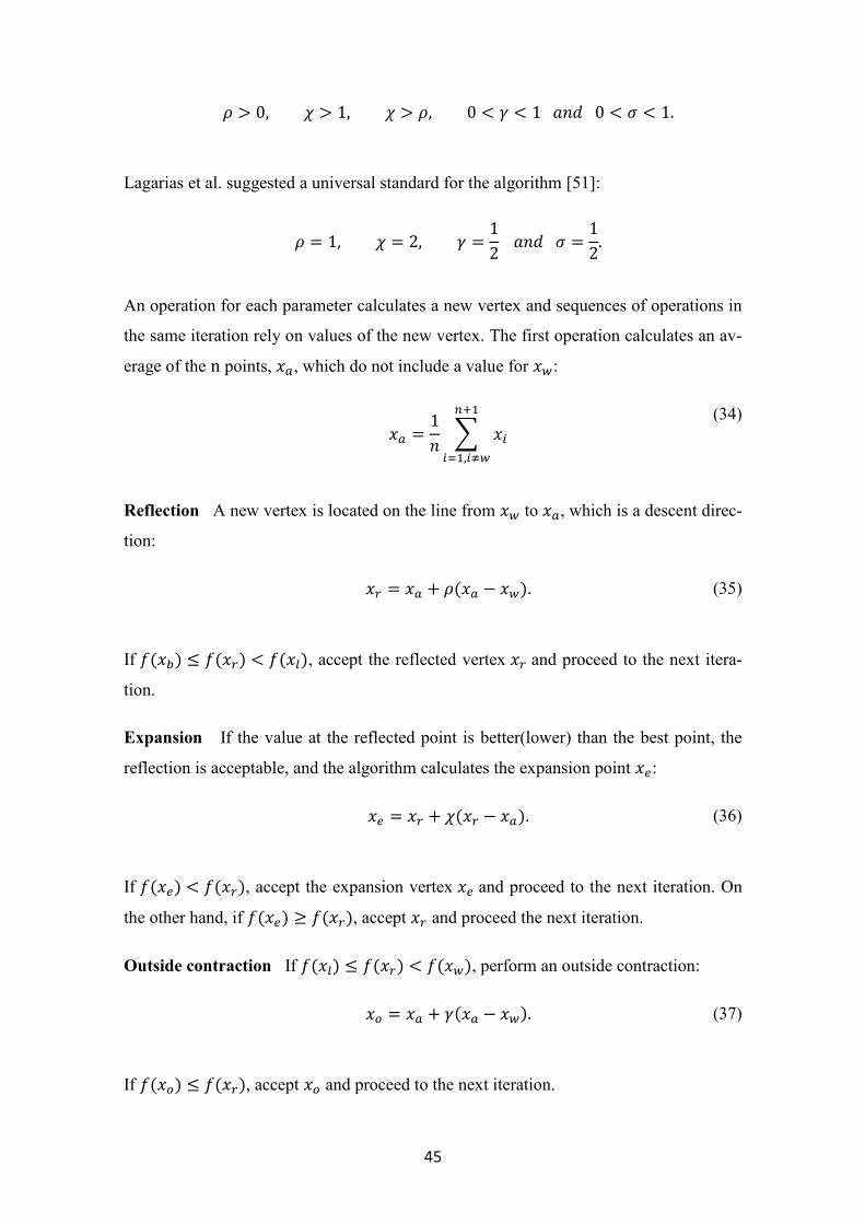
45
𝜌 > 0, 𝜒 > 1, 𝜒 > 𝜌, 0 < 𝛾 < 1 𝑎𝑛𝑑 0 < 𝜎 < 1.
Lagarias et al. suggested a universal standard for the algorithm [51]:
𝜌 = 1, 𝜒 = 2, 𝛾 =1
2 𝑎𝑛𝑑 𝜎 =
1
2.
An operation for each parameter calculates a new vertex and sequences of operations in
the same iteration rely on values of the new vertex. The first operation calculates an av-
erage of the n points, 𝑥𝑎, which do not include a value for 𝑥𝑤:
34 𝑥𝑎 =1
𝑛∑ 𝑥𝑖
𝑛+1
𝑖=1,𝑖≠𝑤
(34)
Reflection A new vertex is located on the line from 𝑥𝑤 to 𝑥𝑎, which is a descent direc-
tion:
35 𝑥𝑟 = 𝑥𝑎 + 𝜌(𝑥𝑎 − 𝑥𝑤). (35)
If 𝑓(𝑥𝑏) ≤ 𝑓(𝑥𝑟) < 𝑓(𝑥𝑙), accept the reflected vertex 𝑥𝑟 and proceed to the next itera-
tion.
Expansion If the value at the reflected point is better(lower) than the best point, the
reflection is acceptable, and the algorithm calculates the expansion point 𝑥𝑒:
36 𝑥𝑒 = 𝑥𝑟 + 𝜒(𝑥𝑟 − 𝑥𝑎). (36)
If 𝑓(𝑥𝑒) < 𝑓(𝑥𝑟), accept the expansion vertex 𝑥𝑒 and proceed to the next iteration. On
the other hand, if 𝑓(𝑥𝑒) ≥ 𝑓(𝑥𝑟), accept 𝑥𝑟 and proceed the next iteration.
Outside contraction If 𝑓(𝑥𝑙) ≤ 𝑓(𝑥𝑟) < 𝑓(𝑥𝑤), perform an outside contraction:
37 𝑥𝑜 = 𝑥𝑎 + 𝛾(𝑥𝑎 − 𝑥𝑤). (37)
If 𝑓(𝑥𝑜) ≤ 𝑓(𝑥𝑟), accept 𝑥𝑜 and proceed to the next iteration.

46
Inside contraction If 𝑓(𝑥𝑤) ≤ 𝑓(𝑥𝑟), perform an inside contraction:
38 𝑥𝑐 = 𝑥𝑎 − 𝛾(𝑥𝑎 − 𝑥𝑤). (38)
If 𝑓(𝑥𝑐) ≤ 𝑓(𝑥𝑤), accept 𝑥𝑐 and proceed to the next iteration.
Shrinkage A new vertex is accepted only after the expansion is successful. Otherwise
previously reflected points are accepted for the next iteration. If reflection, expansion and
contraction fail, an operation shrinkage performs. This operation absorbs all vertices ex-
cluding the best one:
39 𝑥𝑖 = 𝑥𝑏 + 𝜌(𝑥𝑖 − 𝑥𝑏). (39)
3.3 Constrained optimization
Many optimization problems have certain variables which must be satisfied before eval-
uating an optimality condition and before reliability is ensured. The physical laws for the
conservation of mass and Kirchhoff’s voltage and current are representative constraints
[52]. These can be either equality or inequality conditions. The constrained optimization
is relatively more difficult and expensive to get an optimization result than the uncon-
strained optimization. Forms of the equality and inequality constraints are the same as
Equation (22).
The constrained optimization can be largely distinguished by the type of objective and
constraint functions and solution methods: linear, integer, quadratic, nonlinear and dy-
namic programming. It is most common for algorithms to be required to convert an opti-
mization problem with simple constraints into unconstrained problems.
This study only considers the nonlinear constrained optimization, due to a type of objec-
tive function for the estimating hydrodynamic dynamics. The interior point method and
the sequential quadratic programming method are especially discussed in the following
subchapters.

47
3.3.1 Interior point method
The interior point method is a group of algorithms which solves both linear and nonlinear
convex optimization problems. This method finds solutions with the barrier function,
which is based on the penalty method, to make constraints simple.
As many algorithms do so, an idea is initiated from solving linear problems. The simplex
method, which handles vertices of the polytope defined by the constraints, had been the
only available one for decades since the 1940s [53]. Because the simplex method does
not use a polynomial, it requires a lot of time to reach an optimal value through visiting
many vertices [54]. Since Neumann introduced a concept of the interior point method, it
has been continuously updated and progressed. Karmarkar applied a polynomial into his
algorithm, which is based on Khachiyan’s ellipsoid algorithm and is 50 times faster than
the simplex method [55,56]. Gill et al. found that the classical barrier function is similar
with the Karmarkar’s equation and it can be applied to not only to linear problems but
also other problems, such as quadratic and nonlinear programming [57].
An overview of the interior point method for nonlinear optimization is described in the
following. Equation (22) can be transformed by applying the slack variables 𝑠 [58]:
40 𝑚𝑖𝑛 𝑓(𝑥) , 𝑠𝑢𝑏𝑗𝑒𝑐𝑡 𝑡𝑜
𝑐𝐸(𝑥) = 0
𝑐𝐼(𝑥) − 𝑠 = 0
𝑠 ≥ 0.
(40)
The general inequality constraints 𝑐𝐼(𝑥) ≤ 0 is replaced by the slack variables s ≥ 0.
However, the constraints are still complex and it is required to be simpler using the barrier
problem:
41 𝑚𝑖𝑛𝑥,𝑠
𝑓(𝑠) − 𝜇 ∑𝑙𝑜𝑔 𝑠𝑖
𝑚
𝑖=1
, 𝑠𝑢𝑏𝑗𝑒𝑐𝑡 𝑡𝑜
𝑐𝐸(𝑥) = 0
𝑐𝐼(𝑥) − 𝑠 = 0
(41)
where μ is a positive penalty parameter and the slack variable 𝑠 is assumed to be positive.
The barrier problem finds a solution for a sequence of positive barrier parameters, which
converges to zero.

48
The algorithm applies one of two types of searching directions at each iteration [59]:
- A direct step, also known as in the Newton step, in (𝑥, 𝑠), by using the KKT
equations and the primal-dual method for the linear approximation.
- A conjugate gradient step, by using a trust-region method.
The ‘fmincon’ solver attempts to take a direct step firstly. However, if it is not successful,
it searches direction with a conjugate gradient step. This process happens when the ap-
proximate problem is not locally convex.
The KKT equation for the nonlinear programming is [37]:
42 𝛻𝑓(𝑥) − 𝐴𝐸
𝑇(𝑥)𝑦 − 𝐴𝐼𝑇(𝑥)𝑧 = 0
𝑆𝑧 − 𝜇𝑒 = 0
𝑐𝐸(𝑥) = 0
𝑐𝐼(𝑥) − 𝑠 = 0,
(42)
with 𝜇 = 0, 𝑠 ≥ 0 and 𝑧 ≥ 0. Where ∇𝑓(𝑥) is the gradient of 𝑓:
43 𝛻𝑓(𝑥) = (𝜕𝑓(𝑥)
𝜕𝑥1,𝜕𝑓(𝑥)
𝜕𝑥2, … ,
𝜕𝑓(𝑥)
𝜕𝑥𝑛)𝑇
(43)
𝐴𝐸(𝑥) and 𝐴𝐼(𝑥) are the Jacobian matrices, first-order partial derivatives for matrices, for
functions of equality constraints and inequality constraints, respectively:
44 𝐴(𝑥) = 𝛻𝑐(𝑥) = (𝛻𝑐1(𝑥), 𝛻𝑐2(𝑥), 𝛻𝑐3(𝑥), … , 𝛻𝑐𝑚(𝑥)),
𝑤𝑖𝑡ℎ 𝑐: ℝ𝑛 → ℝ𝑚,
(44)
and 𝑦 and 𝑧 are corresponding Lagrange multipliers. 𝑆 and 𝑍 are diagonal matrices and 𝑒
is a vector of ones, with the same size as the inequality constraint.
The primal-dual system for equation (42) by applying Newton’s method is

49
45
[ 𝛻𝑥𝑥
2 ℒ 0 −𝐴𝐸𝑇(𝑥) −𝐴𝐼
𝑇(𝑥)
0 𝑍 0 𝑆𝐴𝐸(𝑥) 0 0 0𝐴𝐼(𝑥) −𝐼 0 0 ]
[
𝑝𝑥
𝑝𝑠
𝑝𝑦
𝑝𝑧
] = −
[ 𝛻𝑓(𝑥) − 𝐴𝐸
𝑇(𝑥) − 𝐴𝐼𝑇(𝑥)
𝑆𝑧 − 𝜇𝑒𝑐𝐸(𝑥)
𝑐𝐼(𝑥) − 𝑠 ]
(45)
where ℒ is the Lagrangian equation for corresponding variables (41):
46 ℒ(𝑥, 𝑠, 𝑦, 𝑧) = 𝑓(𝑥) − 𝑦𝑇𝑐𝐸(𝑥) − 𝑧𝑇(𝑐𝐼(𝑥) + 𝑠). (46)
Next iterations can be calculated after determining the corresponding steps 𝑝 =
(𝑝𝑥, 𝑝𝑠, 𝑝𝑦, 𝑝𝑧):
47 𝑥+ = 𝑥 + 𝛼𝑠
𝑚𝑎𝑥𝑝𝑥
𝑠+ = 𝑠 + 𝛼𝑠𝑚𝑎𝑥𝑝𝑠
𝑦+ = 𝑦 + 𝛼𝑧𝑚𝑎𝑥𝑝𝑦
𝑧+ = 𝑧 + 𝛼𝑧𝑚𝑎𝑥𝑝𝑧 ,
(47)
where 𝛼𝑠𝑚𝑎𝑥 and 𝛼𝑧
𝑚𝑎𝑥 are boundary rules, which monitor descent directions toward
lower bounds, known as the boundary rule:
48 𝛼𝑠
𝑚𝑎𝑥 = 𝑚𝑎𝑥{𝛼 ∈ (0,1): 𝑠 + 𝛼𝑝𝑠 ≥ (1 − 𝜏)𝑠}
𝛼𝑧𝑚𝑎𝑥 = 𝑚𝑎𝑥{𝛼 ∈ (0,1): 𝑧 + 𝛼𝑝𝑧 ≥ (1 −)𝑧} ,
𝑤𝑖𝑡ℎ 𝜏 ∈ (0,1).
(48)
The equations above are a concept of the interior point method. In a real situation, the
algorithm is struggling with nonconvexities and nonlinearities.
3.3.2 Sequential quadratic programming method
The sequential quadratic programming (SQP) method is an effective technique for small-
and medium-sized nonlinear programming problems. It generates steps by solving quad-
ratic subproblems [37]. Since Wilson proposed the first SQP method, this method has
become one of the most successful methods for constrained nonlinear optimization prob-
lems [60]. As with most optimization methods, the SQP is a huge concept, which is com-
posed of multiple specific algorithms [61].
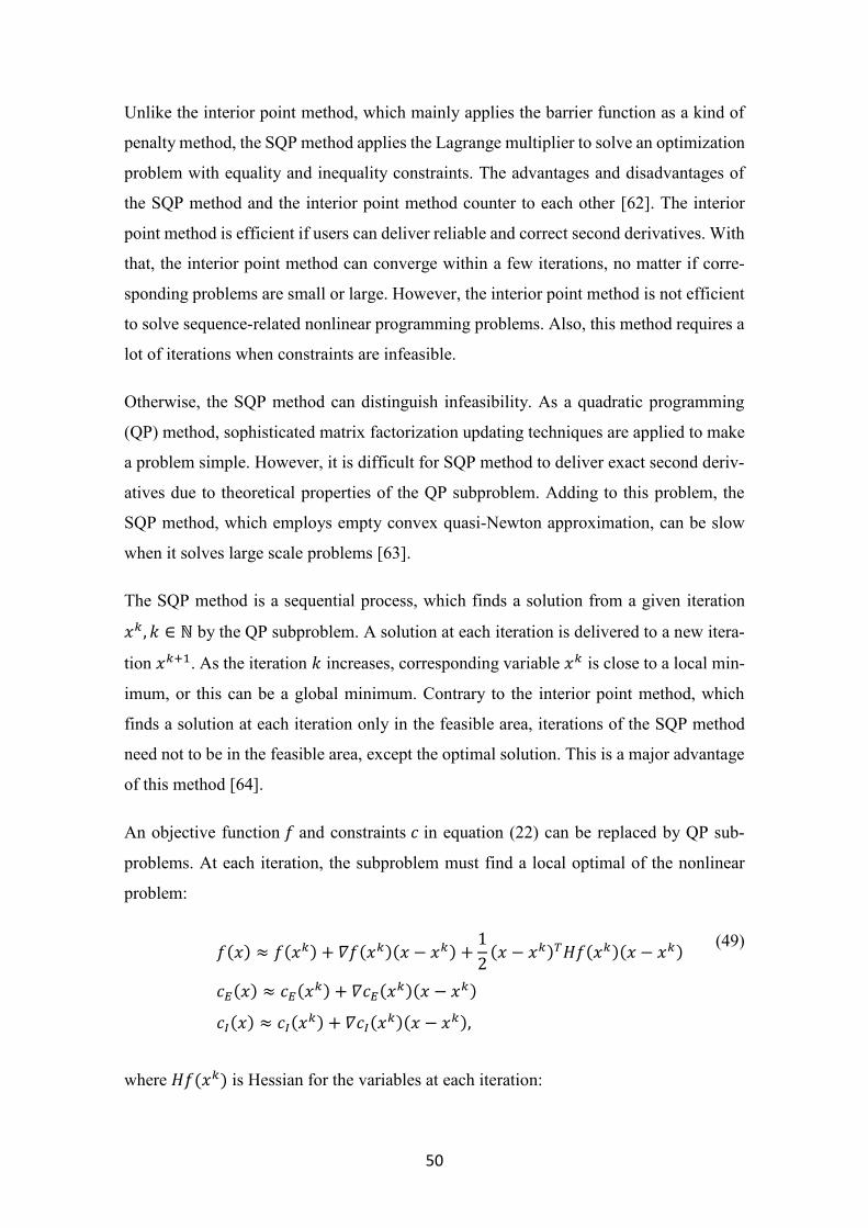
50
Unlike the interior point method, which mainly applies the barrier function as a kind of
penalty method, the SQP method applies the Lagrange multiplier to solve an optimization
problem with equality and inequality constraints. The advantages and disadvantages of
the SQP method and the interior point method counter to each other [62]. The interior
point method is efficient if users can deliver reliable and correct second derivatives. With
that, the interior point method can converge within a few iterations, no matter if corre-
sponding problems are small or large. However, the interior point method is not efficient
to solve sequence-related nonlinear programming problems. Also, this method requires a
lot of iterations when constraints are infeasible.
Otherwise, the SQP method can distinguish infeasibility. As a quadratic programming
(QP) method, sophisticated matrix factorization updating techniques are applied to make
a problem simple. However, it is difficult for SQP method to deliver exact second deriv-
atives due to theoretical properties of the QP subproblem. Adding to this problem, the
SQP method, which employs empty convex quasi-Newton approximation, can be slow
when it solves large scale problems [63].
The SQP method is a sequential process, which finds a solution from a given iteration
𝑥𝑘 , 𝑘 ∈ ℕ by the QP subproblem. A solution at each iteration is delivered to a new itera-
tion 𝑥𝑘+1. As the iteration 𝑘 increases, corresponding variable 𝑥𝑘 is close to a local min-
imum, or this can be a global minimum. Contrary to the interior point method, which
finds a solution at each iteration only in the feasible area, iterations of the SQP method
need not to be in the feasible area, except the optimal solution. This is a major advantage
of this method [64].
An objective function 𝑓 and constraints 𝑐 in equation (22) can be replaced by QP sub-
problems. At each iteration, the subproblem must find a local optimal of the nonlinear
problem:
49 𝑓(𝑥) ≈ 𝑓(𝑥𝑘) + 𝛻𝑓(𝑥𝑘)(𝑥 − 𝑥𝑘) +1
2(𝑥 − 𝑥𝑘)𝑇𝐻𝑓(𝑥𝑘)(𝑥 − 𝑥𝑘)
𝑐𝐸(𝑥) ≈ 𝑐𝐸(𝑥𝑘) + 𝛻𝑐𝐸(𝑥𝑘)(𝑥 − 𝑥𝑘)
𝑐𝐼(𝑥) ≈ 𝑐𝐼(𝑥𝑘) + 𝛻𝑐𝐼(𝑥
𝑘)(𝑥 − 𝑥𝑘),
(49)
where 𝐻𝑓(𝑥𝑘) is Hessian for the variables at each iteration:

51
50 (𝐻𝑓(𝑥))𝑖𝑗 =𝜕2𝑓(𝑥)
𝜕𝑥𝑖𝜕𝑥𝑗, 1 ≤ 𝑖, 𝑗 ≤ 𝑛,
(50)
and it will be replaced by an approximation 𝐵𝑘 as the Quasi-Newton method. Based on
Equation (49) and substituting 𝐵𝑘 = 𝐻𝑓(𝑥𝑘) and 𝑑(𝑥) = 𝑥 − 𝑥𝑘 , the QP subproblem
can be written as follows:
51 𝑚𝑖𝑛 𝛻𝑓(𝑥𝑘)𝑇𝑑(𝑥) +1
2𝑑(𝑥)𝑇𝐵𝑘𝑑(𝑥)
𝑜𝑣𝑒𝑟 𝑑(𝑥) ∈ ℝ𝑛
𝑠𝑢𝑏𝑗𝑒𝑐𝑡 𝑡𝑜 𝑐𝐸(𝑥𝑘) + 𝛻𝑐𝐸(𝑥𝑘)𝑇𝑑(𝑥) = 0
𝑐𝐼(𝑥𝑘) + 𝛻𝑐𝐼(𝑥
𝑘)𝑇𝑑(𝑥) ≤ 0.
(51)
The objective function in Equation (51) can be converted to a function of Lagrangian
equation ℒ:
52 𝑚𝑖𝑛 𝛻ℒ(𝑥𝑘 , 𝑦𝑘, 𝑧𝑘)𝑇𝑑(𝑥) +1
2𝑑(𝑥)𝑇𝐻ℒ(𝑥𝑘 , 𝑦𝑘, 𝑧𝑘)𝑑(𝑥)
𝑜𝑣𝑒𝑟 𝑑(𝑥) ∈ ℝ𝑛
𝑠𝑢𝑏𝑗𝑒𝑐𝑡 𝑡𝑜 𝑐𝐸(𝑥𝑘) + 𝛻𝑐𝐸(𝑥𝑘)𝑇𝑑(𝑥) = 0
𝑐𝐼(𝑥𝑘) + 𝛻𝑐𝐼(𝑥
𝑘)𝑇𝑑(𝑥) ≤ 0.
(52)
53 ℒ(𝑥, 𝑦, 𝑧) = 𝑓(𝑥) + 𝑦𝑇𝑐𝐸(𝑥) + 𝑧𝑇𝑐𝐼(𝑥) (53)
where 𝑦𝑘 and 𝑧𝑘 are the corresponding Lagrange multipliers for equality and inequality
constraints, respectively. When variables at a certain iteration 𝑥𝑘 are a local minimum x∗,
Equation (22) is

52
54 𝑚𝑖𝑛 ℒ(𝑥∗, 𝑦∗, 𝑧∗)
𝑜𝑣𝑒𝑟 𝑥 ∈ ℝ𝑛 , 𝑠𝑢𝑏𝑗𝑒𝑐𝑡 𝑡𝑜
𝑐𝐸(𝑥) = 0
𝑐𝐼(𝑥) ≤ 0
(54)
To ensure equivalence between Equation (51) and Equation (52), the following conditions
must be satisfied:
- If there are no inequality constraints, both equations are equivalent.
- In case of the fully constrained case, the Lagrange multiplier for the inequality
constraint 𝑧𝑘 must be 0.
The first-order necessary optimally conditions, which are important to determine a local
minimum are:
55 𝛻ℒ(𝑥∗, 𝑦∗, 𝑧∗) = 𝛻𝑓(𝑥∗) + 𝛻𝑐𝐸𝑓(𝑥∗)𝑦∗ + 𝛻𝑐𝐼𝑓(𝑥∗)𝑧∗ = 0
𝑤𝑖𝑡ℎ 𝑥∗ ∈ ℝ𝑛, 𝑦∗ ∈ ℝ𝑚 𝑎𝑛𝑑 𝑧∗ ∈ ℝ𝑝,
(55)
and the second order sufficient optimality conditions are the following:
- The columns of 𝐺(𝑥∗) are linearly independent,
- Strict complementary slackness holds at 𝑥∗, and
- The Hessian of the Lagrangian is positive definite, when 𝑥 is positive definite
on the null space of 𝐺(𝑥∗)𝑇
where 𝐺(𝑥∗) is a matrix of first derivatives for equality constraints 𝑐 and strict comple-
mentary slackness 𝑔:
56 𝐺(𝑥∗) = (𝛻𝑐𝐸1(𝑥), 𝛻𝑐𝐸2(𝑥), … , 𝛻𝑐𝐸𝑚(𝑥), 𝛻𝑔𝑖1(𝑥),… , 𝛻𝑔𝑖𝑞𝑥(𝑥)) , 𝑠𝑢𝑏𝑗𝑒𝑐𝑡 𝑡𝑜
𝑔𝑖(𝑥∗)𝑧∗ = 0, 1 ≤ 𝑖 ≤ 𝑝
𝑧∗ > 0, 𝑖 ∈
(56)
where 𝐼𝑎𝑐(𝑥∗) is known as a set of active constraints:

53
57 𝐼𝑎𝑐(𝑥
∗) = {𝑖 ∈ {1,… , 𝑝} | 𝑐𝐼𝑖(𝑥) = 0} . (57)
The optimization process terminates and returns an optimal solution 𝑥∗ when the iteration
𝑥𝑘 for the QP subproblem is the same with the active constraints at the iteration 𝑥𝑘:
58 𝑚𝑖𝑛 𝛻𝑓(𝑥𝑘)𝑇𝑑(𝑥) +1
2𝑑(𝑥)𝑇𝐵𝑘𝑑(𝑥) ,
𝑠𝑢𝑏𝑗𝑒𝑐𝑡 𝑡𝑜 𝛻𝑐𝐼(𝑥𝑘)𝑇𝑑(𝑥) + 𝑐𝐼(𝑥
𝑘) = 0.
(58)

54
4. Coefficients estimation using mathematical opti-
mization
4.1 Introduction
This chapter introduces an overall procedure to estimate hydrodynamic derivatives for a
ship’s hull using mathematical optimization algorithms and a ship’s equations of motion
which are described in previous chapters. Optimization problems, such as variables, and
objective function and constraints, are demonstrated according to the sequence of the
mathematical optimization. Also, basic information on reference data and ways to acquire
them will be provided.
Aims of this chapter can be mainly distinguished into two parts. The first one is that sea
trial data can be suitable for reference data for the optimization process. Success of this
aim can be determined how simulation data using optimized coefficients are close to the
reference data. If it is satisfactory, the second aim finds which algorithm is the most
proper one to the mathematical optimization using sea trial data. With preparation and
verification of the optimization, estimation of hydrodynamic coefficients considering trim
and draught conditions are tried in the next chapter.
4.2 About the mathematical optimization
The mathematical optimization finds minimums or maximums of an objective function
with certain constraints. Especially for the optimization of hydrodynamic coefficients,
this is a series of processes to acquire optimized coefficients which return similar manoeu-
vring characteristics with certain reference data. These data can be measured from sea
trials and are essential to set up an objective function and constraints, to compare with
simulation results at each iteration.
Figure 4.1 shows a concept for the optimization process, especially for estimating hydro-
dynamic coefficients. When a user provides reference data, initial coefficients and
lower/upper bounds, an optimization solver finds an optimal solution according to a des-
ignated optimization algorithm. The algorithm calculates a set of hydrodynamic coeffi-
cients, satisfying all constraints, and checks an optimality of the objective faction which
compares simulation data using the coefficients with the reference data. If the objective
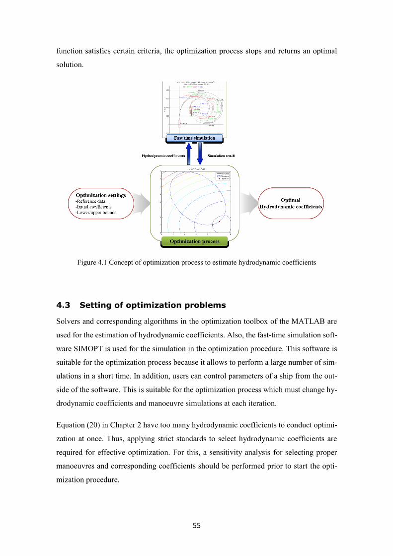
55
function satisfies certain criteria, the optimization process stops and returns an optimal
solution.
Figure 4.1 Concept of optimization process to estimate hydrodynamic coefficients
4.3 Setting of optimization problems
Solvers and corresponding algorithms in the optimization toolbox of the MATLAB are
used for the estimation of hydrodynamic coefficients. Also, the fast-time simulation soft-
ware SIMOPT is used for the simulation in the optimization procedure. This software is
suitable for the optimization process because it allows to perform a large number of sim-
ulations in a short time. In addition, users can control parameters of a ship from the out-
side of the software. This is suitable for the optimization process which must change hy-
drodynamic coefficients and manoeuvre simulations at each iteration.
Equation (20) in Chapter 2 have too many hydrodynamic coefficients to conduct optimi-
zation at once. Thus, applying strict standards to select hydrodynamic coefficients are
required for effective optimization. For this, a sensitivity analysis for selecting proper
manoeuvres and corresponding coefficients should be performed prior to start the opti-
mization procedure.

56
A general definition of the sensitivity analysis is a process of checking how the change
of the input information affects the output change. The sensitivity analysis enables figur-
ing out proper variables, a set of hydrodynamic coefficients for this study, for the optimi-
zation. Normally this can be divided into two types: global sensitivity and local sensitivity.
In most cases, a term ‘sensitivity’ refers to the local sensitivity and it can also be divided
into direct method, indirect method and green function method, and this study applies the
indirect method for the sensitivity analysis [18].
The indirect method is the simplest way to find sensitivity, and it calculates correlation
between a parameter and corresponding function using finite difference approximation:
59 |𝜕𝑓
𝜕𝑥𝑖| ≈ |
𝑓(𝑥𝑖 + ∆𝑥𝑖) − 𝑓(𝑥𝑖)
∆𝑥𝑖| , 𝑤𝑖𝑡ℎ 𝑖 = 1,… , 𝑛.
(59)
This study applies three manoeuvres: straight motion with constant speed, zig-zag ma-
noeuvre and turning manoeuvre. Sensitivity is calculated from changes of manoeuvre
characteristics according to the change of each parameter in a certain range.
The calculated sensitivities may differ due to size or unit of corresponding parameters.
Thus, it is required to conduct normalization to compare them at once. The normalization
means adjusting values measured on different scales to common scale. Z-scores, min-
max method and normalization by decimal scaling are well known methods.
The min-max normalization performs a linear transformation of the original data. This
method converts a value 𝑑 of a group of parameters 𝑃 to 𝑑’ in the new range [new.min
(𝑃), new.max (𝑃)], as follows:
60 𝑑′ =(𝑑 − 𝑚𝑖𝑛(𝑃)) ∗ (𝑛𝑒𝑤.𝑚𝑎𝑥(𝑃) − 𝑛𝑒𝑤.𝑚𝑖𝑛(𝑃))
𝑚𝑎𝑥(𝑃) − 𝑚𝑖𝑛 (𝑃)+ 𝑛𝑒𝑤.𝑚𝑖𝑛(𝑃).
(60)
If the desired range is from 0 to 1, Equation (60) can be converted simply as shown below:
61 𝑑′ =𝑑 − 𝑚𝑖𝑛 (𝑝)
𝑚𝑎𝑥(𝑝) − 𝑚𝑖𝑛 (𝑝)
(61)
As described above, the sensitivity analysis and the normalization are divided into three
steps for the stepwise optimization for estimating hydrodynamic coefficients. Target co-
efficients for each sensitivity analysis are chosen according to basic characteristics of

57
each manoeuvre: straight motion, steer a ship with small rudder angle and large rudder
angle. Added mass which are combined with acceleration components in Equation (20)
are excluded in the sensitivity analysis and corresponding normalization due to their com-
plexity. Table 4.1 shows results of the sensitivity analysis and the normalization.
The first step compares only coefficients in the force acting on the X-axis, and coefficients
𝑋𝑢𝑢 and 𝑋𝑢4 are the values of interest. For the second step, coefficients
𝑋𝑣𝑟 and linear components acting on Y- and Z-axis are compared with the small rudder
angle. The result sows that the coefficient 𝑁𝑢𝑣 is the biggest influence on zig-zag ma-
noeuvre and 𝑋𝑣𝑟 has no influence. The last step compares 𝑋𝑣𝑟 and the remaining nonlin-
ear components acting on Y- and Z- axis. From this, coefficients 𝑋𝑣𝑟, 𝑌𝑣𝑟 , 𝑁𝑟𝑟 and 𝑁𝑣𝑣
are chosen as manipulate variables. Figure 4.2 shows corresponding results of the sensi-
tivity analysis.
Table 4.1 Results of sensitivity analysis on hydrodynamic coefficients
Coefficients Step 1
Straight motion
Step 2
Zig-zag, 10 deg.
Step 3
Turning, 35 deg.
𝑋𝑣𝑟 0 0 0.0890
𝑋𝑢𝑢 1.0000
𝑋𝑢4 0.5587
𝑋𝑢𝑣𝑣𝑣 0
𝑌𝑢𝑣 0.0096
𝑌𝑢𝑟 0.0476
𝑁𝑢𝑣 1.0000
𝑁𝑢𝑟 0.0930
𝑌𝑟𝑟 0
𝑌𝑣𝑣 0
𝑌𝑣𝑟𝑡 0
𝑌𝑣𝑟 0.0675
𝑌𝑣𝑣𝑣𝑟 0.0088
𝑌𝑟𝑟𝑡 0
𝑌𝑣𝑣𝑡 0
𝑌4𝑣2𝑟𝑡 0
𝑁𝑣𝑟 0
𝑁𝑟𝑟𝑡 0
𝑁𝑣𝑣𝑡 0
𝑁𝑟𝑟 1.0000
𝑁𝑣𝑣 0.2213
𝑁𝑣4𝑟2 0.0264
𝑁𝑣𝑟𝑡 0
𝑁5𝑣3𝑟𝑡 0

58
(a) Sensitivity analysis for straight motion
(b) Sensitivity analysis for zig-zag manoeuvre
(c) Sensitivity analysis for turning manoeuvre
Figure 4.2 Results of sensitivity analysis on hydrodynamic coefficients

59
Table 4.2 summarizes the variables for each optimization step.
Table 4.2 Variables on each optimization step
Step Coefficients Remarks
1 𝑋𝑢𝑢 , 𝑋𝑢4 Straight motion
2 𝑌𝑢𝑣 , 𝑌𝑢𝑟 , 𝑁𝑢𝑣 , 𝑁𝑢𝑟 Zig-zag manoeuvre (10 deg.): Small rudder angle
3 𝑋𝑣𝑟 , 𝑌𝑣𝑟 , 𝑁𝑟𝑟 , 𝑁𝑣𝑣 Turning manoeuvre (35 deg.): Large rudder angle
4.4 Sea trial measurements and corrections for reference
data
The objective function and constraints are written using reference data from sea trials,
which were taken only for this thesis. The author planned and managed the whole process
of the trials. The measurements are taken from a training ship of G/T 6,686t. The objective
function compares trajectories of the reference data and trajectories of a simulation result
which is based on calculated coefficients at each iteration. The constraint function com-
pares manoeuvre characteristics of the same manoeuvre with the objective function. All
of constraints are set as equality constraints. The biggest advantage of this idea is that
optimization requires measurement data for ship’s trajectories and this enables simple
procedures during the sea trial measurements. Table 4.3 shows details of the reference
vessel and equation (62) shows a concept of the objective function:
Table 4.3 Details of the reference vessel for comparing optimization algorithms
Type of vessel Training ship
Length overall [m] 117.20
Length between perpendiculars [m] 104.42
Breadth [m] 17.80
Depth at upper deck [m] 10.85
Gross tonnage 6,686.00
Type of main engine MAN B&W 6L42MC/ME
Maximum power [KW] 6,052.54
Maximum speed [kts] 18.40
Propeller Single, right-handed, fixed-pitch
Draught forward (sea trial) [m] 6.10
Draught aft (sea trial) [m] 6.10
Displacement (sea trial) [ton] 6,741.70

60
62 𝑓𝑜𝑏𝑗𝑒𝑐𝑡𝑖𝑣𝑒 = ∑|(𝑝𝑜𝑠. 𝑥𝑖
𝑟𝑒𝑓𝑒𝑟𝑒𝑛𝑐𝑒− 𝑝𝑜𝑠. 𝑥𝑖
𝑖𝑡𝑒𝑟𝑎𝑡𝑖𝑜𝑛)|
𝑖
+
∑|(𝑝𝑜𝑠. 𝑦𝑖𝑟𝑒𝑓𝑒𝑟𝑒𝑛𝑐𝑒
− 𝑝𝑜𝑠. 𝑦𝑖𝑖𝑡𝑒𝑟𝑎𝑡𝑖𝑜𝑛)|
𝑖
.
(62)
Sea trials are carried out in accordance with recommendations of IMO and ITTC [23,27],
as stated in the subchapter 2.2. Table 4.4 shows environmental conditions for sea trials.
Time histories of position, heading, speed, rudder angle, propeller revolution and envi-
ronmental information are measured during the sea trial. Table 4.5 and Table 4.6 show
time histories for the zig-zag and turning manoeuvre, respectively.
Table 4.4 Summary of conditions for sea trials
Data1 Data2
Manoeuvre ZZ10 TC35
Latitude 34.98N 34.95N
Longitude 129.12E 129.09E
Heading [deg] 210 220
RPM [‰] 681 681
Draught fore [m] 6.10 6.10
Draught mid [m] 6.10 6.10
Draught aft [m] 6.10 6.10
Wind direction [deg] 286 286
Wind speed [kts] 5.8 5.8
Current direction [deg] 225 225
Current speed [kts] 0.5 0.5
Water depth [m] 83 89
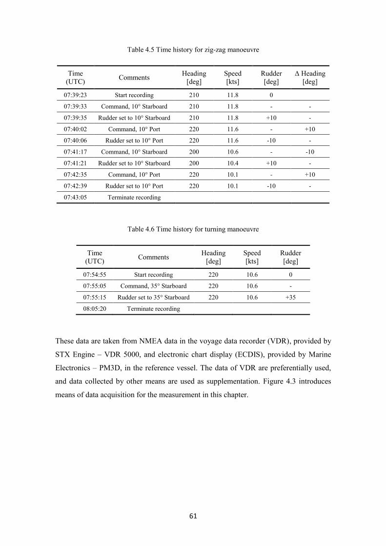
61
Table 4.5 Time history for zig-zag manoeuvre
Time
(UTC) Comments
Heading
[deg]
Speed
[kts]
Rudder
[deg]
Δ Heading
[deg]
07:39:23 Start recording 210 11.8 0
07:39:33 Command, 10° Starboard 210 11.8 - -
07:39:35 Rudder set to 10° Starboard 210 11.8 +10 -
07:40:02 Command, 10° Port 220 11.6 - +10
07:40:06 Rudder set to 10° Port 220 11.6 -10 -
07:41:17 Command, 10° Starboard 200 10.6 - -10
07:41:21 Rudder set to 10° Starboard 200 10.4 +10 -
07:42:35 Command, 10° Port 220 10.1 - +10
07:42:39 Rudder set to 10° Port 220 10.1 -10 -
07:43:05 Terminate recording
Table 4.6 Time history for turning manoeuvre
Time
(UTC) Comments
Heading
[deg]
Speed
[kts]
Rudder
[deg]
07:54:55 Start recording 220 10.6 0
07:55:05 Command, 35° Starboard 220 10.6 -
07:55:15 Rudder set to 35° Starboard 220 10.6 +35
08:05:20 Terminate recording
These data are taken from NMEA data in the voyage data recorder (VDR), provided by
STX Engine – VDR 5000, and electronic chart display (ECDIS), provided by Marine
Electronics – PM3D, in the reference vessel. The data of VDR are preferentially used,
and data collected by other means are used as supplementation. Figure 4.3 introduces
means of data acquisition for the measurement in this chapter.

62
(a) Simplified Voyage Data Recorder (S-VDR)
(b) Electronic Chart DISplay (ECDIS)
Figure 4.3 Means of data acquisition: S-VDR and ECDIS [65]
Sea trials should be carried out in calm weather conditions, as the situation allows. How-
ever, it is hard to conduct sea trials with desired weather conditions due to many reasons.
In case of ship’s manoeuvrability assessment, the trial results can be corrected, if the
minimum weather conditions for the criteria requirements are not met. In this study, for

63
the purpose of comparing optimization algorithms, environmental effects on the meas-
urement data are corrected according to the IMO recommendation [23].
This correction starts form the results of the turning manoeuvre. The turning circle test
results are useful to measure the magnitude and direction of current. At the time of the
sea trial, the ship’s dynamic information, such as position and heading, should be col-
lected until at least 720° of heading change. Two half circles which can be measured after
180° of heading change from the initial heading are used for estimating magnitude and
direction of the environmental effect, especially for current. Equation (63) shows the local
current velocity 𝑉𝑖 which can be defined by the two positions, (𝑥1𝑖, 𝑦1𝑖, 𝑡1𝑖) and
(𝑥2𝑖, 𝑦2𝑖 , 𝑡2𝑖), from the half circles:
63 𝑉𝑖 =(𝑥2𝑖 − 𝑥1𝑖 , 𝑦2𝑖 − 𝑦1𝑖)
(𝑡2𝑖 − 𝑡1𝑖).
(63)
From sets of local velocity, the estimated current velocity can be calculated from Equation
(64):
64 𝑉𝑐 =1
𝑛∑𝑉𝑖
𝑛
𝑖=1
=1
𝑛∑
(𝑥2𝑖 − 𝑥1𝑖 , 𝑦2𝑖 − 𝑦1𝑖)
(𝑡2𝑖 − 𝑡1𝑖)
𝑛
𝑖=1
. (64)
The magnitude of the current velocity can be calculated as
65 𝑉𝑐 = |𝑉𝑐|. (65)
The final corrected trajectories of the measurement data can be obtained from the follow-
ing:
66 𝑥′(𝑡) = 𝑥(𝑡) − 𝑉𝑐𝑡, (66)
where 𝑥(𝑡) is the measured position vector and 𝑥′(𝑡) is the corrected position of the ship
and 𝑥′(𝑡) = 𝑥(𝑡) at 𝑡 = 0.
Figure 4.4 compares the measured sea trial trajectory and the corrected trajectory. Cor-
rection values are obtained from the measurement of turning manoeuvre, and they are

64
also applied to the measurement of the zig-zag manoeuvre. Both trajectories are corrected
environmental effects which force the ship shift to the north-east direction.
Optimizations are carried out with six conditions using four algorithms: a solver ‘fmincon’
uses the interior point and the SQP algorithms, a solver ‘fminunc’ uses the Quasi-Newton
algorithm and a solver ‘fminsearch’ uses the Nelder-Mead algorithm. Algorithms for con-
strained optimization, the interior point and the SQP are also be divided to optimizations
with and without constraints. As mentioned in Table 4.2, stepwise optimization is carried
out in the order of the straight motion, the zig-zag manoeuvre and the turning manoeuvre.
Step 2 and Step 3 change coefficients which are already optimized in the previous step(s),
prior to starting the main optimization process.
(a) (b)
Figure 4.4 Comparisons of measurement data and corrected data
Table 4.7 shows detailed conditions of the optimization for this chapter. Initial values can
be calculated from the Clarke estimation. Lower and upper bounds apply close value to 0
or 10 times greater than the initial value. Step 1 conducts optimization without constraints,
due to simple manoeuvre and relatively small number of variables. Step 2 and 3 apply
constraints using manoeuvre characteristics, such as overshoot angle and tactical diameter,
if applicable.

65
Table 4.7 Detailed conditions of optimization
Step 1 Step 2 Step 3
Solver (Algorithm)
fmincon (interior-point, SQP)
fminunc (Quasi-Newton)
fminsearch (Nelder-Mead)
Initial values
𝑋𝑢𝑢 -0.0458 𝑌𝑢𝑣 -1.5336 𝑋𝑣𝑟 1.0225
𝑋𝑢4 -0.3490 𝑌𝑢𝑟 0.3245 𝑌𝑣𝑟 1.7265
𝑁𝑢𝑣 -0.5796 𝑁𝑟𝑟 0.1079
𝑁𝑢𝑟 -0.2429 𝑁𝑣𝑣 0.8633
Lower bounds
𝑋𝑢𝑢 -0.4000 𝑌𝑢𝑣 -15.3360 𝑋𝑣𝑟 0.0001
𝑋𝑢4 -3.0000 𝑌𝑢𝑟 0.0001 𝑌𝑣𝑟 0.0001
𝑁𝑢𝑣 -5.7960 𝑁𝑟𝑟 0.0001
𝑁𝑢𝑟 -0.2429 𝑁𝑣𝑣 0.0001
Upper bounds
𝑋𝑢𝑢 -0.0001 𝑌𝑢𝑣 -0.0001 𝑋𝑣𝑟 10.0000
𝑋𝑢4 -0.0001 𝑌𝑢𝑟 3.2450 𝑌𝑣𝑟 17.0000
𝑁𝑢𝑣 -0.0001 𝑁𝑟𝑟 1.0790
𝑁𝑢𝑟 -0.0001 𝑁𝑣𝑣 8.6330
Objective function Track difference
Straight motion Zig-zag, 10 deg. Turning, 35 deg.
Constraints
(if applicable) - First overshoot Tactical diameter
4.5 Optimization results
Table 4.8 shows Clarke coefficients, which are initial values in the optimization process
and results of all optimizations at once. Optimized coefficients of step 1, constant speed
with straight motion, are not different from the Clarke coefficients. In case of the step 2,
the zig-zag manoeuvre with a rudder angle of 10 degrees, coefficients of yaw moment (𝑁)
have more variation than coefficients of sway force (𝑌). It relates to the results of the
sensitivity analysis in the subchapter 4.2 that sensitivity for coefficients of yaw moment
are greater than the others. Also, it is shown that the algorithms of constrained optimiza-
tion, the interior point and the SQP, have different results according to the presence of
constraints. This will be discussed later with simulation results using optimized coeffi-
cients. The results of step 3 also show that the coefficient 𝑁𝑟𝑟 which is the most sensible
one has the biggest variation among variables.

66
Table 4.8 Summarization of Clarke coefficients and optimized coefficients
Coefficients Clarke IP
(con)
IP
(uncon)
SQP
(con)
SQP
(uncon) QN NM
𝑋𝑢𝑢 -0.0458 -0.0403 -0.0403 -0.0458 -0.0458 -0.0408 -0.0397
𝑋𝑢4 -0.3490 -0.3490 -0.3490 -0.2323 -0.2323 -0.3480 -0.3575
𝑌𝑢𝑣 -1.5336 -1.3006 -1.5283 -1.7185 -1.4252 -1.5257 -1.5188
𝑌𝑢𝑟 0.3245 0.2888 0.2905 0.1780 0.3020 0.2970 0.2919
𝑁𝑢𝑣 -0.5796 -2.0583 -2.2262 -1.5637 -0.9484 -0.6141 -0.6293
𝑁𝑢𝑟 -0.2429 -0.7399 -0.7112 -0.4707 -0.2257 -0.1429 -0.1429
𝑋𝑣𝑟 1.0225 0.7680 0.4968 1.2000 0.0001 0.4167 1.0225
𝑌𝑣𝑟 1.7265 2.4636 1.4223 1.6924 2.4582 1.8311 1.6099
𝑁𝑟𝑟 0.1079 0.0623 0.3461 0.1105 0.0172 0.3496 0.1079
𝑁𝑣𝑣 0.8633 0.6450 0.6232 1.0169 5.5060 0.6120 1.8633
Remarks
IP: Interior point
SQP: Sequential quadratic programming
QN: Quasi-Newton
NM: Nelder-Mead
con: Constrained
uncon: Unconstrained
Table 4.9 shows manoeuvre characteristics of the reference data and simulations results
using Clarke coefficients and optimized coefficients. Manoeuvre characteristics of the
reference data are acquired from the measurement data which have been already corrected
environmental effects. For the Clarke coefficients, simulation results are directly reflected
in the results table. The simulation results using optimized coefficients are summarized
step-by step to see the change of manoeuvring characteristics with step progress.
The selected manoeuvres for the simulation are the same as the optimization process:
straight motion with constant speed, zig-zag manoeuvre with a rudder angle of 10 degrees
and turning manoeuvre with a hard rudder. Manoeuvre characteristics are as follows: ratio
of sailed distance for the straight motion to ship’s length between perpendiculars
(Way/LPP), first and second overshoot angles for the zig-zag manoeuvre and advance
and tactical diameter for the turning manoeuvre.

67
Table 4.9 Manoeuvre characteristics of reference data and simulation results
Straight Zig-zag, 10 degrees Turning, 35degrees
Way/LPP Overshoot 1 Overshoot 2 Advance Tactical dia.
Reference 23.4768 7.2 12.7 298.0000 399.5000
Clarke 23.0435 3.1 4.7 298.0729 430.2624
IP, step 1 23.4626 3.3 4.7 300.2329 433.8391
IP (con), step 2 23.4190 7.0 15.2 286.0168 353.8225
IP (con), step 3 23.4227 6.5 13.5 291.2115 389.6643
IP (uncon), step 2 23.4200 7.6 16.0 268.0846 336.7742
IP (uncon), step 3 23.4224 6.9 14.8 296.1285 393.6173
SQP, step 1 23.4435 3.3 4.6 299.8891 432.6124
SQP (con), step 2 23.1895 8.8 18.2 245.5009 300.8476
SQP (con), step 3 23.1896 8.6 17.9 247.0885 305.0851
SQP (uncon), step 2 22.6818 9.0 19.3 217.6083 270.2148
SQP (uncon), step 3 23.0396 5.9 8.7 329.6871 590.2585
QN, step 1 23.4268 3.3 4.6 299.9692 433.4675
QN, step 2 23.3352 7.3 13.0 222.3280 289.4011
QN, step 3 23.3541 5.6 8.8 285.9273 435.4688
NM, step 1 23.4787 3.3 4.6 300.3715 433.6262
NM, step 2 23.3100 7.9 14.1 219.6220 283.4635
NM, step 3 23.3281 6.8 11.0 246.2697 361.6117
Remarks
IP: Interior point
SQP: Sequential quadratic programming
QN: Quasi-Newton
NM: Nelder-Mead
con: Constrained
uncon: Unconstrained
Figure 4.5 compares the manoeuvre characteristic, Way/LPP for the reference data and
the simulation results. As shown in Table 4.9, Way/LPP for all simulations including
results of Clarke coefficients are close to the reference data. Results for step 2 of the
unconstrained SQP are the worst, and it is 3.38% lower than the reference data. It is shown
that optimized coefficients of later steps can also affect a manoeuvrability of the straight
motion.

68
Figure 4.5 Comparison of optimization algorithms: straight motion
For step 2, as shown in Figure 4.6, the difference between the manoeuvre characteristics
is larger than step 1. Results of the interior point and the Quasi-Newton algorithms are
closer to the reference data than the rest results. In case of the interior point algorithm,
the difference between constrained and unconstrained optimization is not large.
The results of step 3 show no significant difference from the results of step 2. The interior
point and the Quasi-Newton algorithms have high similarity with the reference data, and
in the order of the Nelder-Mead and the SQP algorithms. However, for the advance, the
value for the Clarke coefficients is already close to the reference data. Because of this,
advance values for the simulation using coefficients of step 1 are also close to the refer-
ence data. This means that the advance is not proper parameter to compare algorithms for
this reference data. In addition, the advance should not be used as constraints.

69
Figure 4.6 Comparison of optimization algorithms: zig-zag manoeuvre
Figure 4.7 Comparison of optimization algorithms: turning manoeuvre
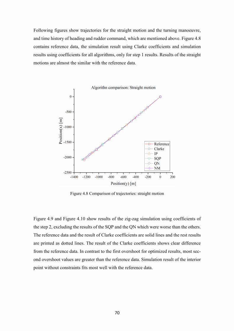
70
Following figures show trajectories for the straight motion and the turning manoeuvre,
and time history of heading and rudder command, which are mentioned above. Figure 4.8
contains reference data, the simulation result using Clarke coefficients and simulation
results using coefficients for all algorithms, only for step 1 results. Results of the straight
motions are almost the similar with the reference data.
Figure 4.8 Comparison of trajectories: straight motion
Figure 4.9 and Figure 4.10 show results of the zig-zag simulation using coefficients of
the step 2, excluding the results of the SQP and the QN which were worse than the others.
The reference data and the result of Clarke coefficients are solid lines and the rest results
are printed as dotted lines. The result of the Clarke coefficients shows clear difference
from the reference data. In contrast to the first overshoot for optimized results, most sec-
ond overshoot values are greater than the reference data. Simulation result of the interior
point without constraints fits most well with the reference data.

71
Figure 4.9 Comparison of trajectories: zig-zag motion
Figure 4.10 Comparison of heading change: zig-zag manoeuvre
Figure 4.11 shows results of the turning manoeuvre. Similar with the results of step 2, the
circle of the SQP is significantly greater than both the reference data and other simulation

72
results. As mentioned above, values of the advance are similar with each other excluding
the value of the SQP. For other algorithms, the shape and diameter of the circles are sim-
ilar, but their positions differ.
Figure 4.11 Comparison of trajectories: turning manoeuvre
Figure 4.12 to Figure 4.14 compare results of zig-zag manoeuvre using coefficients for
the results of the optimization step 2 and 3, respectively. In every case, difference of the
second overshoot angel from the reference from the simulation results for the step 3 is
smaller than the ones for the step 2.
Considering the results, the interior point algorithm calculates the best solution for both
constrained and unconstrained optimization. In the next chapter, unconstrained optimiza-
tion with the interior point algorithm will be applied firstly; after that, if corresponding
results are not satisfactory, constrained optimization will be tried.

73
Figure 4.12 Comparison of heading change for optimization steps 2 and 3: Interior point algo-
rithm with constraint
Figure 4.13 Comparison of heading change for optimization steps 2 and 3: Interior point algo-
rithm without constraint

74
Figure 4.14 Comparison of heading change for optimization steps 2 and 3: Nelder-Mead algo-
rithm
Figure 4.15 to Figure 4.17 show the history of iterations for each step. It seems that the
‘fmincon’ solver with the interior point algorithm has found optimal coefficients at the
middle of the whole iterations. However, it takes more iterations to conclude them as a
final solution. This is because of continuously descending gradients of the objective func-
tion. Regularly the algorithm starts an optimization for a certain coefficient from the
lower or upper bound, prominent point in the iteration history, but soon the coefficient
returns to the solution.

75
Figure 4.15 History of iteration: straight motion
Figure 4.16 History of iteration: zig-zag manoeuvre

76
Figure 4.17 History of iterations: turning manoeuvre
4.6 Conclusion
In this chapter, an optimization problem was set up and its verification was carried out.
Also, four optimization algorithms were compared to find the best algorithm for estima-
tion of hydrodynamic coefficients.
The optimization problem consists of variables selection, reference selection for objective
and constraint functions and optimization condition setting. Setting the optimal number
of variables can help in making a more effective and faster optimization process. For this,
optimal variables were selected through comparison of the hydrodynamic coefficients
using sensitivity analysis and normalization. The reference data were borrowed from a
set of sea trial data of a training ship, which were conducted and managed by author. The
raw sea trial data were applied to the final reference data after applying the environmental
influence correction formulas which are provided by IMO. The optimization conditions
were set to six versions using four different algorithms. The optimizations were carried
out stepwise according to the characteristics of each manoeuvre.

77
Most of the optimization results were similar with the reference. This seems to be the
results of proper optimization problem setting and algorithm selection. Specifically, the
optimization results fitted to the reference data in the order of the interior point, the Quasi-
Newton, the Nelder-Mead and the SQP algorithms. In the next chapter, all the optimiza-
tions will be carried out using the interior-point algorithm.

78
5. Coefficients estimation for various trim and
draught conditions
5.1 Introduction
This chapter estimates hydrodynamic coefficients considering various trim and draught
conditions. Firstly, hydrodynamic coefficients are mathematically optimized using sea
trial data with various trim and draught conditions. By utilizing those coefficients and
corresponding trim and draught conditions, new coefficients which are for another trim
and draught condition will be estimated, and simulation results using the new coefficients
will also be compared with their reference data.
5.2 Optimization problems
Details of the reference vessel in this chapter are shown in Table 5.1. The vessel is a 4,500
TEU class container carrier with a length of 294 metres and a maximum draught of 13
metres. Sea trials were carried out in 2012 by Krüger [32].
Table 5.1 Details of the reference vessel
Type of vessel 4,500 TEU class container carrier
Length overall [m] 294.12
Length between perpendiculars [m] 283.20
Breadth, moulded [m] 32.20
Depth, moulded [m] 10.85
Design draught, moulded [m] 12.00
Scantling draught, moulded [m] 13.00
Gross tonnage 53,324.00
Deadweight [ton] 63,510.00
Full load displacement [ton] 82,496.00
Type of main engine MAN B&W 9K90MC-C
Maximum power [KW] 41,040.00
Maximum speed [kts] 23.70
Propeller Single, right-handed, fixed-pitch
Table 5.2 summarizes conditions of each sea trial. All five trials are zig-zag manoeuvres,
and they can be divided into three trim and draught conditions: mean trim 9.35 metres

79
with trim 0.5 metres by stern, mean trim 10 metres with even keel and mean trim 12.875
metres with trim 0.25 metres by stern. Unlike Chapter 4, all simulations used in this chap-
ter consider the environment influence, wind and currents at the time of sea trials. Time
histories for each manoeuvre will be presented in 7.
Table 5.2 Summary of conditions for sea trials
Data1 Data2 Data3 Data4 Data5
Manoeuvre ZZ10P ZZ10S ZZ10S ZZ10P ZZ20S
Latitude 32.8N 32.0N 10.7N 9.7N 9.7N
Longitude 119.9W 117.3W 67.2W 79.6W 79.6W
Heading [deg] 110 110 260 250 250
RPM [‰] 843 620 676 422 422
Draught fore [m] 12.75 12.75 10.00 9.10 9.10
Draught mid [m] 12.55 12.55 10.00 - -
Draught aft [m] 13.00 13.00 10.00 9.60 9.60
Wind direction [deg] 270 310 20 50 50
Wind speed [kts] 12 15 5 15 15
Current direction [deg] 160.47 251.56 169.50 23.62 23.62
Current speed [kts] 1.37 0.88 0.28 1.25 1.55
Water depth [m] >1000 >1000 >1000 >1000 >1000
Table 5.3 shows selection of variables through sensitivity analysis and normalization,
with the same process as in Chapter 4. However, coefficients for steering with a large
rudder angle are excluded from variables because all the measurements are zig-zag ma-
noeuvres. The selected variables are the same as those of Chapter 4.
Table 5.3 Variables on each optimization step
Step Coefficients Remarks
1 𝑋𝑢𝑢 , 𝑋𝑢4 Straight motion
2 𝑌𝑢𝑣 , 𝑌𝑢𝑟 , 𝑁𝑢𝑣 , 𝑁𝑢𝑟 Zig-zag manoeuvre (10 deg.): Small rudder angle
Data 2, 3 and 4 in Table 5.2 which have different trim and draught conditions are opti-
mized first. Table 5.4 summarizes optimization conditions of the data.
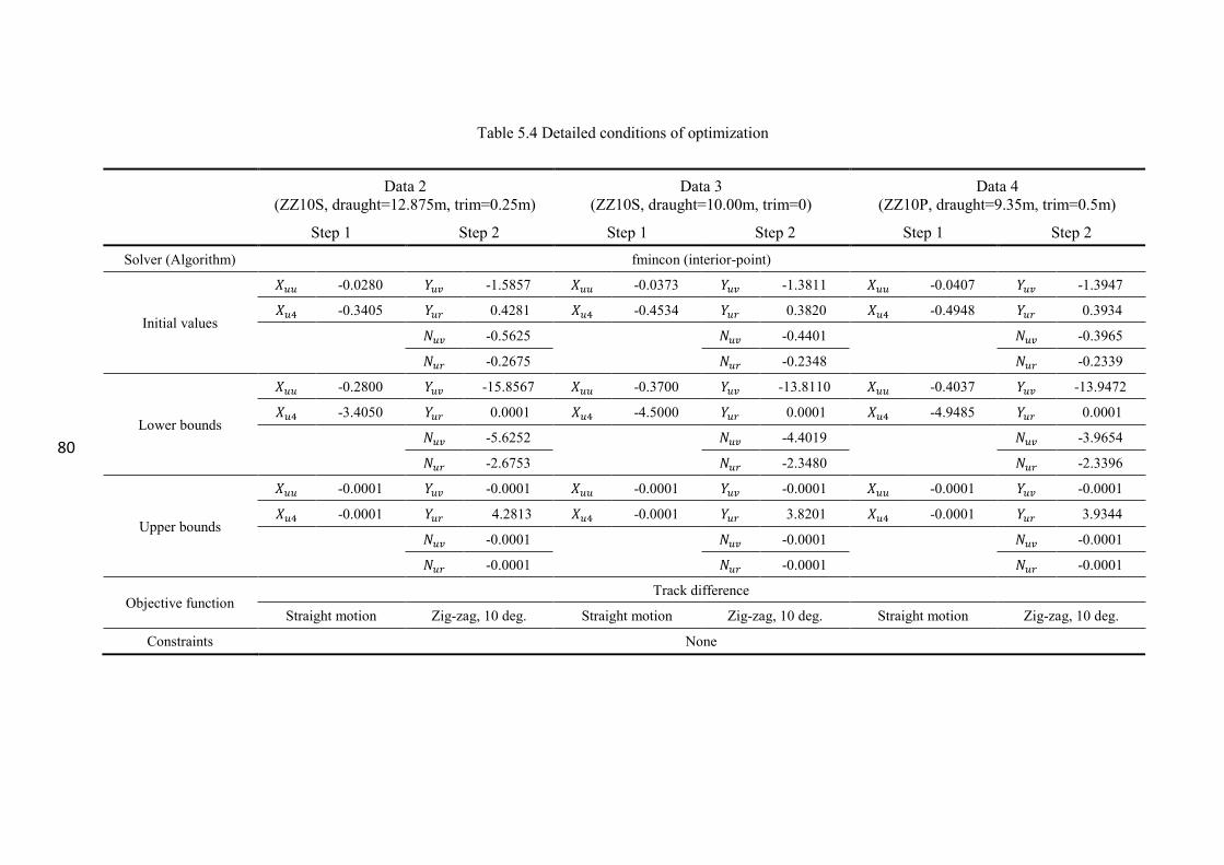
80
Table 5.4 Detailed conditions of optimization
Data 2
(ZZ10S, draught=12.875m, trim=0.25m)
Data 3
(ZZ10S, draught=10.00m, trim=0)
Data 4
(ZZ10P, draught=9.35m, trim=0.5m)
Step 1 Step 2 Step 1 Step 2 Step 1 Step 2
Solver (Algorithm) fmincon (interior-point)
Initial values
𝑋𝑢𝑢 -0.0280 𝑌𝑢𝑣 -1.5857 𝑋𝑢𝑢 -0.0373 𝑌𝑢𝑣 -1.3811 𝑋𝑢𝑢 -0.0407 𝑌𝑢𝑣 -1.3947
𝑋𝑢4 -0.3405 𝑌𝑢𝑟 0.4281 𝑋𝑢4 -0.4534 𝑌𝑢𝑟 0.3820 𝑋𝑢4 -0.4948 𝑌𝑢𝑟 0.3934
𝑁𝑢𝑣 -0.5625
𝑁𝑢𝑣 -0.4401
𝑁𝑢𝑣 -0.3965
𝑁𝑢𝑟 -0.2675 𝑁𝑢𝑟 -0.2348 𝑁𝑢𝑟 -0.2339
Lower bounds
𝑋𝑢𝑢 -0.2800 𝑌𝑢𝑣 -15.8567 𝑋𝑢𝑢 -0.3700 𝑌𝑢𝑣 -13.8110 𝑋𝑢𝑢 -0.4037 𝑌𝑢𝑣 -13.9472
𝑋𝑢4 -3.4050 𝑌𝑢𝑟 0.0001 𝑋𝑢4 -4.5000 𝑌𝑢𝑟 0.0001 𝑋𝑢4 -4.9485 𝑌𝑢𝑟 0.0001
𝑁𝑢𝑣 -5.6252
𝑁𝑢𝑣 -4.4019
𝑁𝑢𝑣 -3.9654
𝑁𝑢𝑟 -2.6753 𝑁𝑢𝑟 -2.3480 𝑁𝑢𝑟 -2.3396
Upper bounds
𝑋𝑢𝑢 -0.0001 𝑌𝑢𝑣 -0.0001 𝑋𝑢𝑢 -0.0001 𝑌𝑢𝑣 -0.0001 𝑋𝑢𝑢 -0.0001 𝑌𝑢𝑣 -0.0001
𝑋𝑢4 -0.0001 𝑌𝑢𝑟 4.2813 𝑋𝑢4 -0.0001 𝑌𝑢𝑟 3.8201 𝑋𝑢4 -0.0001 𝑌𝑢𝑟 3.9344
𝑁𝑢𝑣 -0.0001
𝑁𝑢𝑣 -0.0001
𝑁𝑢𝑣 -0.0001
𝑁𝑢𝑟 -0.0001 𝑁𝑢𝑟 -0.0001 𝑁𝑢𝑟 -0.0001
Objective function Track difference
Straight motion Zig-zag, 10 deg. Straight motion Zig-zag, 10 deg. Straight motion Zig-zag, 10 deg.
Constraints None
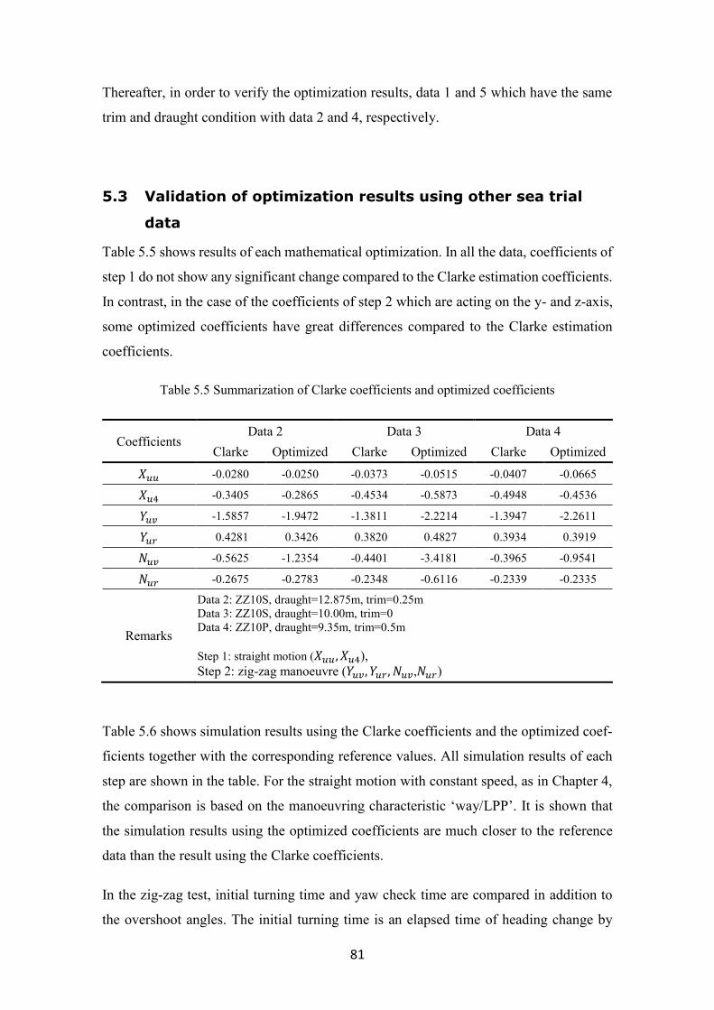
81
Thereafter, in order to verify the optimization results, data 1 and 5 which have the same
trim and draught condition with data 2 and 4, respectively.
5.3 Validation of optimization results using other sea trial
data
Table 5.5 shows results of each mathematical optimization. In all the data, coefficients of
step 1 do not show any significant change compared to the Clarke estimation coefficients.
In contrast, in the case of the coefficients of step 2 which are acting on the y- and z-axis,
some optimized coefficients have great differences compared to the Clarke estimation
coefficients.
Table 5.5 Summarization of Clarke coefficients and optimized coefficients
Coefficients Data 2 Data 3 Data 4
Clarke Optimized Clarke Optimized Clarke Optimized
𝑋𝑢𝑢 -0.0280 -0.0250 -0.0373 -0.0515 -0.0407 -0.0665
𝑋𝑢4 -0.3405 -0.2865 -0.4534 -0.5873 -0.4948 -0.4536
𝑌𝑢𝑣 -1.5857 -1.9472 -1.3811 -2.2214 -1.3947 -2.2611
𝑌𝑢𝑟 0.4281 0.3426 0.3820 0.4827 0.3934 0.3919
𝑁𝑢𝑣 -0.5625 -1.2354 -0.4401 -3.4181 -0.3965 -0.9541
𝑁𝑢𝑟 -0.2675 -0.2783 -0.2348 -0.6116 -0.2339 -0.2335
Remarks
Data 2: ZZ10S, draught=12.875m, trim=0.25m
Data 3: ZZ10S, draught=10.00m, trim=0
Data 4: ZZ10P, draught=9.35m, trim=0.5m
Step 1: straight motion (𝑋𝑢𝑢, 𝑋𝑢4),
Step 2: zig-zag manoeuvre (𝑌𝑢𝑣 , 𝑌𝑢𝑟 , 𝑁𝑢𝑣,𝑁𝑢𝑟)
Table 5.6 shows simulation results using the Clarke coefficients and the optimized coef-
ficients together with the corresponding reference values. All simulation results of each
step are shown in the table. For the straight motion with constant speed, as in Chapter 4,
the comparison is based on the manoeuvring characteristic ‘way/LPP’. It is shown that
the simulation results using the optimized coefficients are much closer to the reference
data than the result using the Clarke coefficients.
In the zig-zag test, initial turning time and yaw check time are compared in addition to
the overshoot angles. The initial turning time is an elapsed time of heading change by
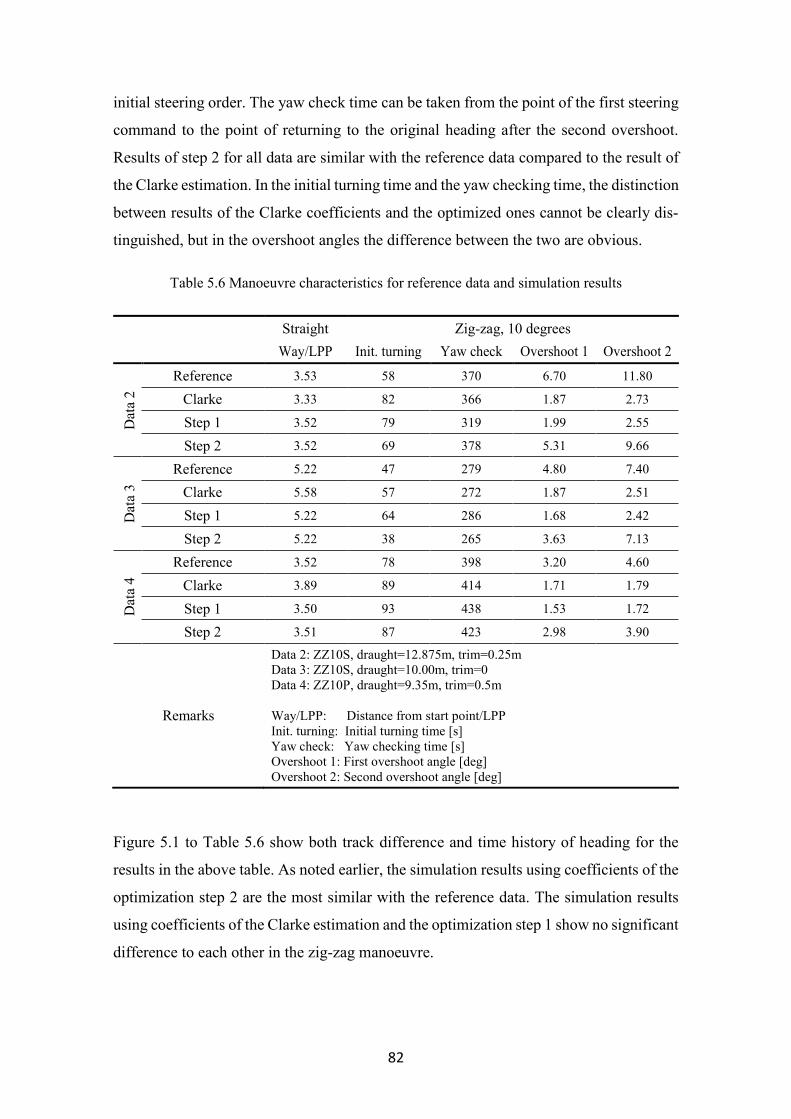
82
initial steering order. The yaw check time can be taken from the point of the first steering
command to the point of returning to the original heading after the second overshoot.
Results of step 2 for all data are similar with the reference data compared to the result of
the Clarke estimation. In the initial turning time and the yaw checking time, the distinction
between results of the Clarke coefficients and the optimized ones cannot be clearly dis-
tinguished, but in the overshoot angles the difference between the two are obvious.
Table 5.6 Manoeuvre characteristics for reference data and simulation results
Straight Zig-zag, 10 degrees
Way/LPP Init. turning Yaw check Overshoot 1 Overshoot 2
Dat
a 2
Reference 3.53 58 370 6.70 11.80
Clarke 3.33 82 366 1.87 2.73
Step 1 3.52 79 319 1.99 2.55
Step 2 3.52 69 378 5.31 9.66
Dat
a 3
Reference 5.22 47 279 4.80 7.40
Clarke 5.58 57 272 1.87 2.51
Step 1 5.22 64 286 1.68 2.42
Step 2 5.22 38 265 3.63 7.13
Dat
a 4
Reference 3.52 78 398 3.20 4.60
Clarke 3.89 89 414 1.71 1.79
Step 1 3.50 93 438 1.53 1.72
Step 2 3.51 87 423 2.98 3.90
Remarks
Data 2: ZZ10S, draught=12.875m, trim=0.25m
Data 3: ZZ10S, draught=10.00m, trim=0
Data 4: ZZ10P, draught=9.35m, trim=0.5m
Way/LPP: Distance from start point/LPP
Init. turning: Initial turning time [s]
Yaw check: Yaw checking time [s]
Overshoot 1: First overshoot angle [deg]
Overshoot 2: Second overshoot angle [deg]
Figure 5.1 to Table 5.6 show both track difference and time history of heading for the
results in the above table. As noted earlier, the simulation results using coefficients of the
optimization step 2 are the most similar with the reference data. The simulation results
using coefficients of the Clarke estimation and the optimization step 1 show no significant
difference to each other in the zig-zag manoeuvre.
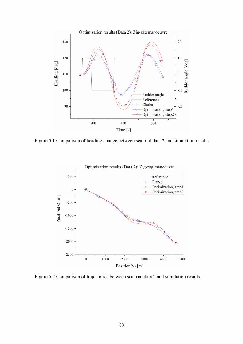
83
Figure 5.1 Comparison of heading change between sea trial data 2 and simulation results
Figure 5.2 Comparison of trajectories between sea trial data 2 and simulation results

84
Figure 5.3 Comparison of heading change between sea trial data 3 and simulation results
Figure 5.4 Comparison of trajectories between sea trial data 3 and simulation results
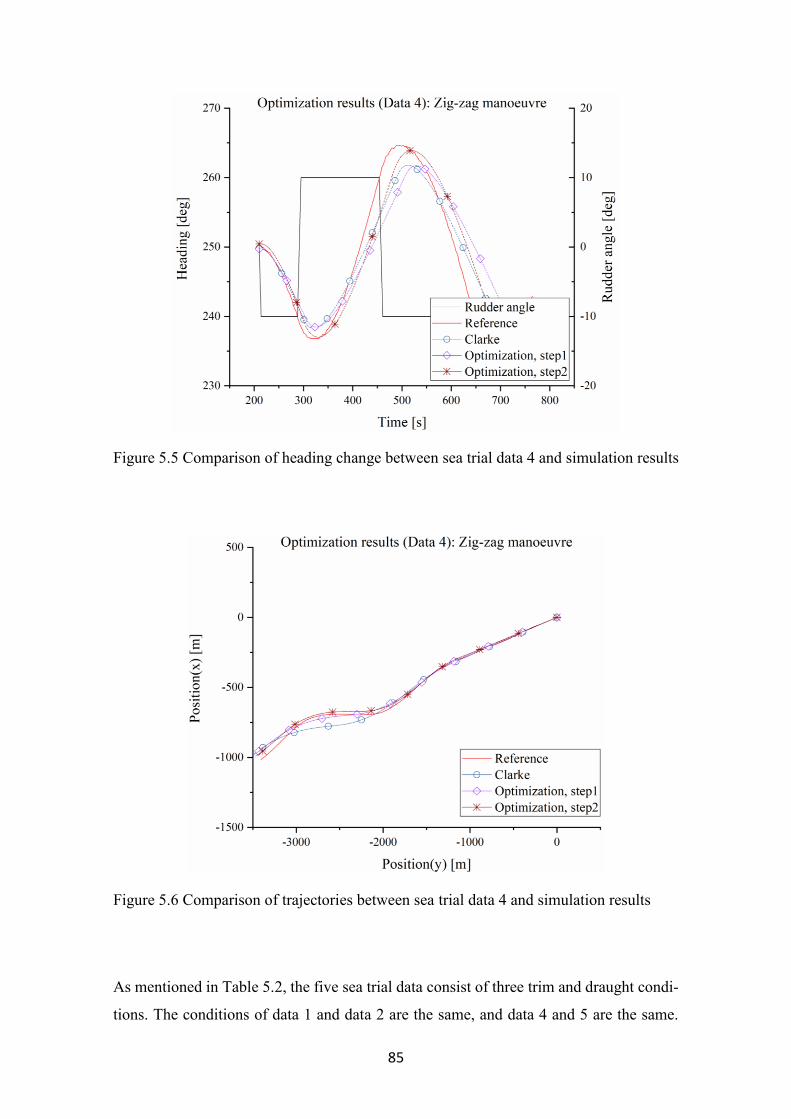
85
Figure 5.5 Comparison of heading change between sea trial data 4 and simulation results
Figure 5.6 Comparison of trajectories between sea trial data 4 and simulation results
As mentioned in Table 5.2, the five sea trial data consist of three trim and draught condi-
tions. The conditions of data 1 and data 2 are the same, and data 4 and 5 are the same.

86
Therefore, as a primary verification for the optimization results presented above, the
tuned coefficients based on the data 2 and the data 4 are used in the simulations for the
data 1 and 5, respectively. This verification is performed using the sea trial data 1 and 5,
and each data is compared with three simulation results. The hydrodynamic coefficients
used in the simulations are as follows:
- calculated coefficients by the formulas of Clarke estimation,
- tuned coefficients based on the data 2 and 4 (provided in Table 5.5) and
- tuned coefficients based on the data 1 and 5.
In other words, this procedure is to verify whether the tuned coefficients of the specific
data can be applied to simulations for other data, if there is sea trial data for the same trim
and draft conditions.
Table 5.7 and Table 5.8 present three sets of coefficients as mentioned above, respectively.
𝑋𝑢𝑢 for the optimization result of the data 1 differs from the Clarke coefficient, while the
result of data 2 is close to the Clarke’s. 𝑋𝑢4, on the other hand, showed that the result of
data 1 is close to the Clarke coefficient. For the coefficients acting on the y- and z-axes,
only 𝑁𝑢𝑣 for the both optimization results show a large difference with the Clarke coeffi-
cients; and for the remaining coefficients, the two optimization results are similar.
Table 5.7 Comparison of optimized coefficients for two sea trial data which have the same trim
and draught condition (Case of the data 1 and 2)
Coefficients Clarke Optimization using
Data 1 Data 2
𝑋𝑢𝑢 -0.0280 -0.0412 -0.0250
𝑋𝑢4 -0.3405 -0.3486 -0.2865
𝑌𝑢𝑣 -1.5857 -1.6097 -1.9472
𝑌𝑢𝑟 0.4281 0.4530 0.3426
𝑁𝑢𝑣 -0.5625 -1.3288 -1.2354
𝑁𝑢𝑟 -0.2675 -0.2740 -0.2783
Remarks
Data 1: ZZ10P, draught=12.875m, trim=0.25m
Data 2: ZZ10S, draught=12.875m, trim=0.25m
Step 1: straight motion (𝑋𝑢𝑢, 𝑋𝑢4),
Step 2: zig-zag manoeuvre (𝑌𝑢𝑣 , 𝑌𝑢𝑟 , 𝑁𝑢𝑣,𝑁𝑢𝑟)

87
Table 5.8 Comparison of optimized coefficients for two sea trial data which have the same trim
and draught condition (Case of the data 4 and 5)
Coefficients Clarke Optimization using
Data 4 Data 5
𝑋𝑢𝑢 -0.0407 -0.0665 -0.0598
𝑋𝑢4 -0.4948 -0.4536 -0.8876
𝑌𝑢𝑣 -1.3947 -2.2611 -2.3852
𝑌𝑢𝑟 0.3934 0.3919 0.4110
𝑁𝑢𝑣 -0.3965 -0.9541 -1.2228
𝑁𝑢𝑟 -0.2339 -0.2335 -0.2548
Remarks
Data 4: ZZ10P, draught=9.35m, trim=0.50m
Data 5: ZZ20S, draught=9.35m, trim=0.50m
Step 1: straight motion (𝑋𝑢𝑢, 𝑋𝑢4),
Step 2: zig-zag manoeuvre (𝑌𝑢𝑣 , 𝑌𝑢𝑟 , 𝑁𝑢𝑣,𝑁𝑢𝑟)
In case of the data 4 and 5, the 𝑋𝑢𝑢 for both optimization results are similar and differ
from the Clarke coefficient. 𝑋𝑢4 for the result of data 5 shows a large difference to the
Clarke coefficient, whereas the coefficient for the result of data 4 is similar with the
Clarke coefficient. The coefficients acting on the y- and z-axes for the both optimization
results are close to each other. Among them, 𝑌𝑢𝑣 and 𝑁𝑢𝑣 show a significant difference
compared with the Clarke coefficients. Comparisons of the manoeuvre results according
to these optimization results are shown in the following table and figures.
Table 5.9 compares manoeuvre characteristics for the simulation results using the coeffi-
cients presented above and for the reference data. Contents for the manoeuvre character-
istics are the same as those in Table 5.6. Each term in the table means as follows:
- ‘Reference’ means manoeuvre characteristic of the sea trial for the data 1.
- ‘Clarke’ represents results of simulation using coefficients calculated by Clarke
estimation.
- ‘Data 1’ shows results of simulation using optimized coefficients based on the
data 1.
- ‘Data 2’ shows results of simulation using optimized coefficients based on the
data 2.
All simulations are carried out under the same conditions as the sea trial data 1. The results
of the straight motion with constant speed show that the simulation result of the data 1 is
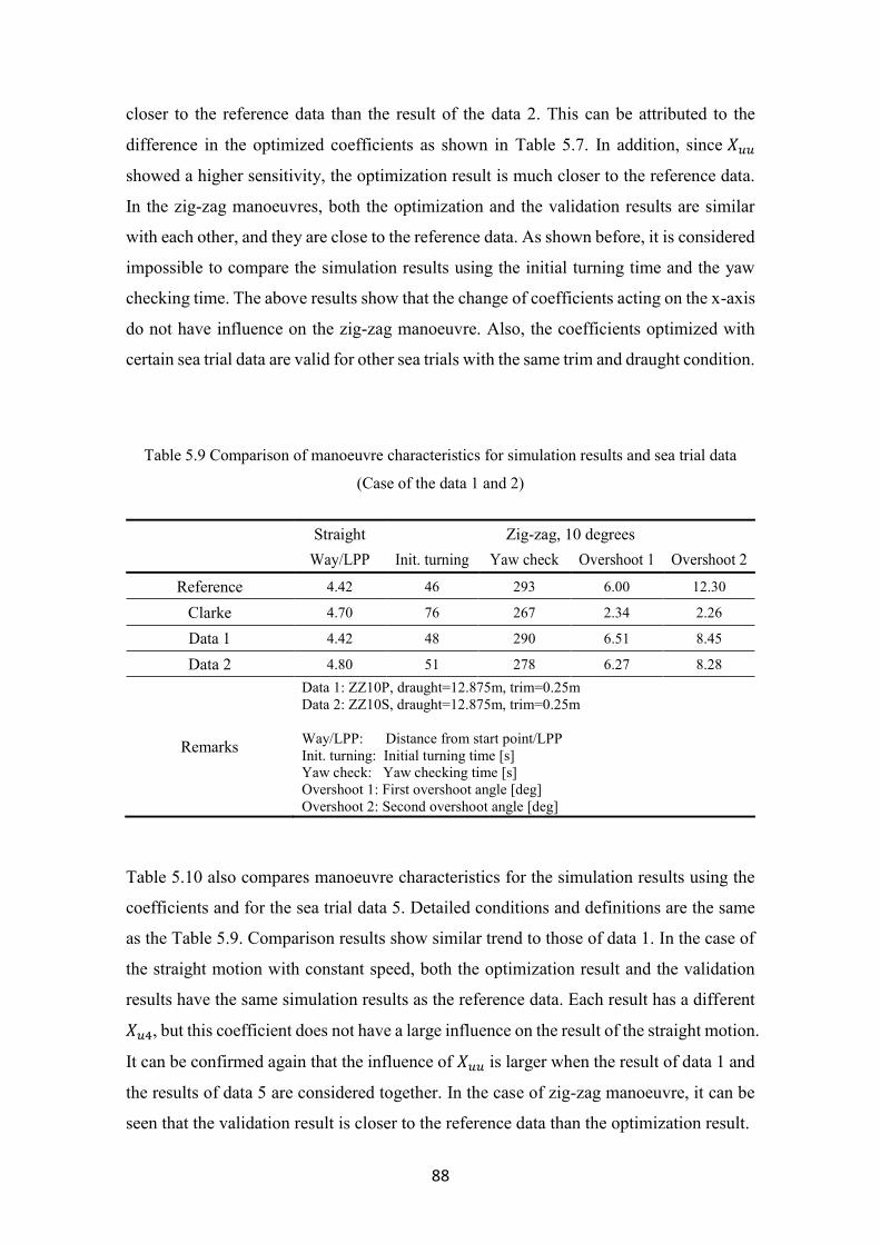
88
closer to the reference data than the result of the data 2. This can be attributed to the
difference in the optimized coefficients as shown in Table 5.7. In addition, since 𝑋𝑢𝑢
showed a higher sensitivity, the optimization result is much closer to the reference data.
In the zig-zag manoeuvres, both the optimization and the validation results are similar
with each other, and they are close to the reference data. As shown before, it is considered
impossible to compare the simulation results using the initial turning time and the yaw
checking time. The above results show that the change of coefficients acting on the x-axis
do not have influence on the zig-zag manoeuvre. Also, the coefficients optimized with
certain sea trial data are valid for other sea trials with the same trim and draught condition.
Table 5.9 Comparison of manoeuvre characteristics for simulation results and sea trial data
(Case of the data 1 and 2)
Straight Zig-zag, 10 degrees
Way/LPP Init. turning Yaw check Overshoot 1 Overshoot 2
Reference 4.42 46 293 6.00 12.30
Clarke 4.70 76 267 2.34 2.26
Data 1 4.42 48 290 6.51 8.45
Data 2 4.80 51 278 6.27 8.28
Remarks
Data 1: ZZ10P, draught=12.875m, trim=0.25m
Data 2: ZZ10S, draught=12.875m, trim=0.25m
Way/LPP: Distance from start point/LPP
Init. turning: Initial turning time [s]
Yaw check: Yaw checking time [s]
Overshoot 1: First overshoot angle [deg]
Overshoot 2: Second overshoot angle [deg]
Table 5.10 also compares manoeuvre characteristics for the simulation results using the
coefficients and for the sea trial data 5. Detailed conditions and definitions are the same
as the Table 5.9. Comparison results show similar trend to those of data 1. In the case of
the straight motion with constant speed, both the optimization result and the validation
results have the same simulation results as the reference data. Each result has a different
𝑋𝑢4, but this coefficient does not have a large influence on the result of the straight motion.
It can be confirmed again that the influence of 𝑋𝑢𝑢 is larger when the result of data 1 and
the results of data 5 are considered together. In the case of zig-zag manoeuvre, it can be
seen that the validation result is closer to the reference data than the optimization result.

89
Table 5.10 Comparison of manoeuvre characteristics for simulation results and sea trial data
(Case of the data 4 and 5)
Straight Zig-zag, 20 degrees
Way/LPP Init. turning Yaw check Overshoot 1 Overshoot 2
Reference 1.96 81 405 5.60 6.10
Clarke 2.15 93 441 3.21 3.25
Data 5 1.95 80 429 6.24 7.15
Data 4 1.93 84 436 5.59 6.26
Remarks
Data 4: ZZ10P, draught=9.35m, trim=0.50m
Data 5: ZZ20S, draught=9.35m, trim=0.50m
Way/LPP: Distance from start point/LPP
Init. turning: Initial turning time [s]
Yaw check: Yaw checking time [s]
Overshoot 1: First overshoot angle [deg]
Overshoot 2: Second overshoot angle [deg]
Figure 5.7 to Figure 5.10 compare the time history of heading for the results from Table
5.9. For data 1, the first overshoot angle for both the optimization result and the validation
result are similar with the reference data, while their second overshoot angle is smaller
than the reference data. For data 5, both the first overshoot and second overshoot angles
for all results are similar with the reference data.
Figure 5.7 Comparison of heading change between sea trial data 1 and various simulations
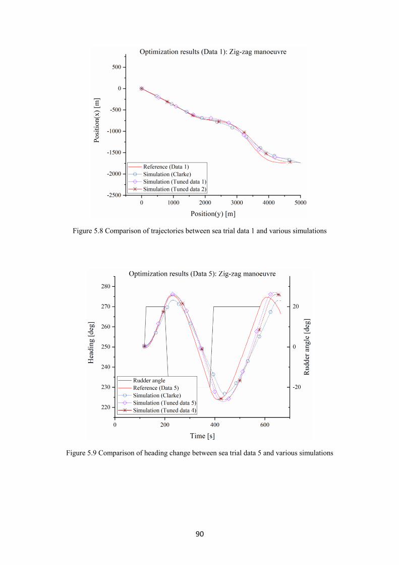
90
Figure 5.8 Comparison of trajectories between sea trial data 1 and various simulations
Figure 5.9 Comparison of heading change between sea trial data 5 and various simulations

91
Figure 5.10 Comparison of trajectories between sea trial data 5 and various simulations
5.4 Estimation of hydrodynamic coefficients considering vari-
ous trim and draught conditions
Based on the optimization results obtained in Subchapter 5.3, estimation of the hydrody-
namic coefficients for a certain trim and draught condition that are not included in the sea
trial conditions are carried out. Also, a corresponding simulation results are compared
with the reference data.
Estimation of the hydrodynamic coefficient considering various trim and draught condi-
tions is basically based on the Clarke estimation formulas. In addition, final coefficients
can be estimated by adding additional correction values using existing optimization re-
sults from sea trials. The validation of the estimated coefficients is performed by consid-
ering the data obtained in the sea trial booklet of the reference vessel.
The coefficients estimation formulas can be constructed as follows. First of all, the esti-
mation formulas which can cope with various trim and draught conditions require a spe-
cific reference trim and draught condition.
In this study, the condition of the data 3 which is 10 metres of the mean draught and even
keel condition is set as a reference condition. The new coefficients can be obtained by
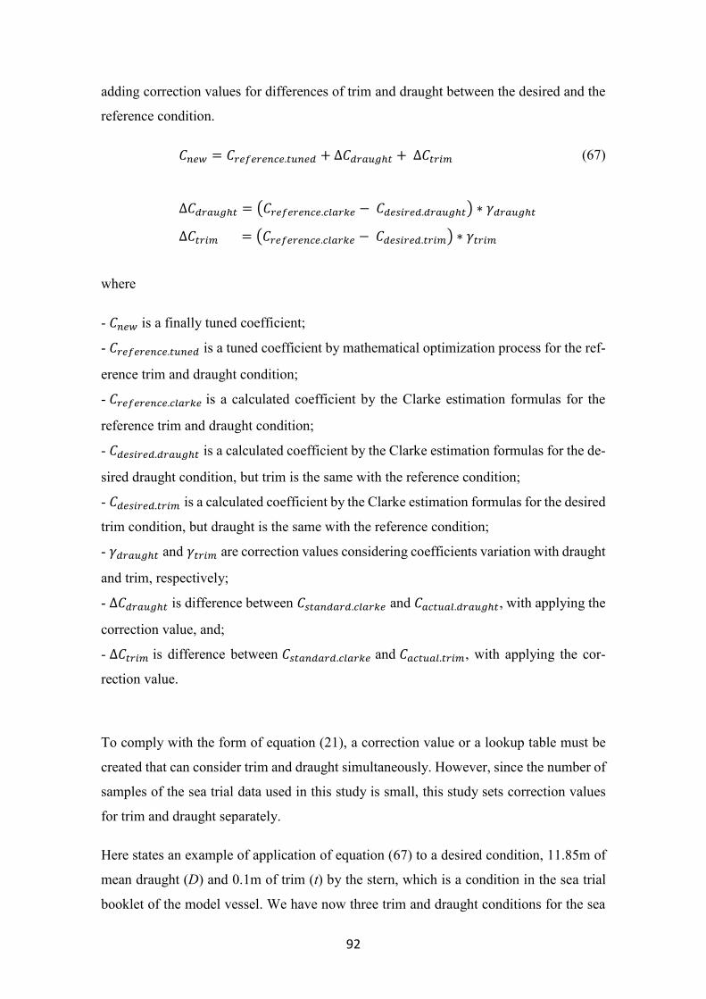
92
adding correction values for differences of trim and draught between the desired and the
reference condition.
67 𝐶𝑛𝑒𝑤 = 𝐶𝑟𝑒𝑓𝑒𝑟𝑒𝑛𝑐𝑒.𝑡𝑢𝑛𝑒𝑑 + ∆𝐶𝑑𝑟𝑎𝑢𝑔ℎ𝑡 + ∆𝐶𝑡𝑟𝑖𝑚
∆𝐶𝑑𝑟𝑎𝑢𝑔ℎ𝑡 = (𝐶𝑟𝑒𝑓𝑒𝑟𝑒𝑛𝑐𝑒.𝑐𝑙𝑎𝑟𝑘𝑒 − 𝐶𝑑𝑒𝑠𝑖𝑟𝑒𝑑.𝑑𝑟𝑎𝑢𝑔ℎ𝑡) ∗ 𝛾𝑑𝑟𝑎𝑢𝑔ℎ𝑡
∆𝐶𝑡𝑟𝑖𝑚 = (𝐶𝑟𝑒𝑓𝑒𝑟𝑒𝑛𝑐𝑒.𝑐𝑙𝑎𝑟𝑘𝑒 − 𝐶𝑑𝑒𝑠𝑖𝑟𝑒𝑑.𝑡𝑟𝑖𝑚) ∗ 𝛾𝑡𝑟𝑖𝑚
(67)
where
- 𝐶𝑛𝑒𝑤 is a finally tuned coefficient;
- 𝐶𝑟𝑒𝑓𝑒𝑟𝑒𝑛𝑐𝑒.𝑡𝑢𝑛𝑒𝑑 is a tuned coefficient by mathematical optimization process for the ref-
erence trim and draught condition;
- 𝐶𝑟𝑒𝑓𝑒𝑟𝑒𝑛𝑐𝑒.𝑐𝑙𝑎𝑟𝑘𝑒 is a calculated coefficient by the Clarke estimation formulas for the
reference trim and draught condition;
- 𝐶𝑑𝑒𝑠𝑖𝑟𝑒𝑑.𝑑𝑟𝑎𝑢𝑔ℎ𝑡 is a calculated coefficient by the Clarke estimation formulas for the de-
sired draught condition, but trim is the same with the reference condition;
- 𝐶𝑑𝑒𝑠𝑖𝑟𝑒𝑑.𝑡𝑟𝑖𝑚 is a calculated coefficient by the Clarke estimation formulas for the desired
trim condition, but draught is the same with the reference condition;
- 𝛾𝑑𝑟𝑎𝑢𝑔ℎ𝑡 and 𝛾𝑡𝑟𝑖𝑚 are correction values considering coefficients variation with draught
and trim, respectively;
- ∆𝐶𝑑𝑟𝑎𝑢𝑔ℎ𝑡 is difference between 𝐶𝑠𝑡𝑎𝑛𝑑𝑎𝑟𝑑.𝑐𝑙𝑎𝑟𝑘𝑒 and 𝐶𝑎𝑐𝑡𝑢𝑎𝑙.𝑑𝑟𝑎𝑢𝑔ℎ𝑡, with applying the
correction value, and;
- ∆𝐶𝑡𝑟𝑖𝑚 is difference between 𝐶𝑠𝑡𝑎𝑛𝑑𝑎𝑟𝑑.𝑐𝑙𝑎𝑟𝑘𝑒 and 𝐶𝑎𝑐𝑡𝑢𝑎𝑙.𝑡𝑟𝑖𝑚, with applying the cor-
rection value.
To comply with the form of equation (21), a correction value or a lookup table must be
created that can consider trim and draught simultaneously. However, since the number of
samples of the sea trial data used in this study is small, this study sets correction values
for trim and draught separately.
Here states an example of application of equation (67) to a desired condition, 11.85m of
mean draught (D) and 0.1m of trim (t) by the stern, which is a condition in the sea trial
booklet of the model vessel. We have now three trim and draught conditions for the sea

93
trials - D=9.35m t=0.5m, D=10.00m t=0m and D=12.875m t=0.25m - and one of them
should be the reference condition. The condition of 10.00m of mean draught and even
keel condition is chosen as the reference condition for this case. Thus equation (67) can
be applied as follows:
68 𝐶𝑛𝑒𝑤,𝐷=11.85𝑚,𝑡=0.1𝑚 = 𝐶𝑡𝑢𝑛𝑒𝑑,𝐷=10.00𝑚,𝑡=0 + ∆𝐶𝑑𝑟𝑎𝑢𝑔ℎ𝑡 + ∆𝐶𝑡𝑟𝑖𝑚
∆𝐶𝑑𝑟𝑎𝑢𝑔ℎ𝑡 = (𝐶𝐶𝑙𝑎𝑟𝑘𝑒,𝐷=10.00𝑚,𝑡=0 − 𝐶𝐶𝑙𝑎𝑟𝑘𝑒,𝐷=11.85𝑚,𝑡=0) ∗ 𝛾𝑑𝑟𝑎𝑢𝑔ℎ𝑡
∆𝐶𝑡𝑟𝑖𝑚 = (𝐶𝐶𝑙𝑎𝑟𝑘𝑒,𝐷=10.00𝑚,𝑡=0 − 𝐶𝐶𝑙𝑎𝑟𝑘𝑒,𝐷=10.00𝑚,𝑡=0.1𝑚) ∗ 𝛾𝑡𝑟𝑖𝑚
[𝛾𝑑𝑟𝑎𝑢𝑔ℎ𝑡
𝛾𝑡𝑟𝑖𝑚] = [
𝐶𝐶𝑙𝑎𝑟𝑘𝑒 𝑑𝑖𝑓𝑓𝑒𝑟𝑒𝑛𝑐𝑒 𝐷1 𝐶𝐶𝑙𝑎𝑟𝑘𝑒 𝑑𝑖𝑓𝑓𝑒𝑟𝑒𝑛𝑐𝑒 𝑡1
𝐶𝐶𝑙𝑎𝑟𝑘𝑒 𝑑𝑖𝑓𝑓𝑒𝑟𝑒𝑛𝑐𝑒 𝐷2 𝐶𝐶𝑙𝑎𝑟𝑘𝑒 𝑑𝑖𝑓𝑓𝑒𝑟𝑒𝑛𝑐𝑒 𝑡2]−1
∗ [𝐶𝑡𝑢𝑛𝑒𝑑 1
𝐶𝑡𝑢𝑛𝑒𝑑 2]
𝐶𝐶𝑙𝑎𝑟𝑘𝑒 𝑑𝑖𝑓𝑓𝑒𝑟𝑒𝑛𝑐𝑒 𝐷1 = 𝐶𝐶𝑙𝑎𝑟𝑘𝑒,𝐷=10.00𝑚,𝑡=0 − 𝐶𝐶𝑙𝑎𝑟𝑘𝑒,𝐷=9.35𝑚,𝑡=0
𝐶𝐶𝑙𝑎𝑟𝑘𝑒 𝑑𝑖𝑓𝑓𝑒𝑟𝑒𝑛𝑐𝑒 𝐷2 = 𝐶𝐶𝑙𝑎𝑟𝑘𝑒,𝐷=10.00𝑚,𝑡=0 − 𝐶𝐶𝑙𝑎𝑟𝑘𝑒,𝐷=12.875𝑚,𝑡=0
𝐶𝐶𝑙𝑎𝑟𝑘𝑒 𝑑𝑖𝑓𝑓𝑒𝑟𝑒𝑛𝑐𝑒 𝑡1 = 𝐶𝐶𝑙𝑎𝑟𝑘𝑒,𝐷=10.00𝑚,𝑡=0 − 𝐶𝐶𝑙𝑎𝑟𝑘𝑒,𝐷=10.00𝑚,𝑡=0.5𝑚
𝐶𝐶𝑙𝑎𝑟𝑘𝑒 𝑑𝑖𝑓𝑓𝑒𝑟𝑒𝑛𝑐𝑒 𝑡2 = 𝐶𝐶𝑙𝑎𝑟𝑘𝑒,𝐷=10.00𝑚,𝑡=0 − 𝐶𝐶𝑙𝑎𝑟𝑘𝑒,𝐷=10.00𝑚,𝑡=0.25𝑚
𝐶𝑡𝑢𝑛𝑒𝑑 1 = 𝐶𝑡𝑢𝑛𝑒𝑑,𝐷=10.00𝑚,𝑡=0 − 𝐶𝑡𝑢𝑛𝑒𝑑,𝐷=9.35𝑚,𝑡=0.5𝑚
𝐶𝑡𝑢𝑛𝑒𝑑 2 = 𝐶𝑡𝑢𝑛𝑒𝑑,𝐷=10.00𝑚,𝑡=0 − 𝐶𝑡𝑢𝑛𝑒𝑑,𝐷=12.875𝑚,𝑡=0.25𝑚
(68)
For the coefficients acting on the 𝑥-axis, 𝑋𝑢𝑢 and 𝑋𝑢4, are affected by nominal resistance
and nominal speed, and estimation of them in this case can be provided by second order
curve fitting from three sets of tuned coefficients. Figure 5.11 shows results of curve
fitting and Table 5.11 presents calculated correction values for the coefficients to be esti-
mated.
Table 5.11 Correction values for estimation formulae which are based on three sea trial meas-
urements
Correction value Remarks
𝑋𝑢𝑢 [-0.0037, 0.0952, -0.6305] Second order fitting
[B2, B1, Intercept] 𝑋𝑢4 [0.0955, -2.0531, 10.3964]
𝛾𝑑𝑟𝑎𝑢𝑔ℎ𝑡 [-1.3953, 0.8239, 15.4710, 10.0599] for
[𝑌𝑢𝑣, 𝑌𝑢𝑟, 𝑁𝑢𝑣, 𝑁𝑢𝑟] 𝛾𝑡𝑟𝑖𝑚 [-0.3713, -11.2893, 224.6883, -184.9057]

94
Figure 5.11 Results of curve fitting for 𝑋𝑢𝑢 and 𝑋𝑢4
Table 5.12 presents environmental conditions for the corresponding sea trial for valida-
tion of the estimation formulae, and it is named as ‘Data 6’.
Table 5.12 Environmental conditions for the sea trial for validation of the estimation formulae
Data6
Manoeuvre ZZ20S
Heading [deg] 176.6
Draught fore [m] 11.80
Draught aft [m] 11.90
Wind direction [deg] 263.8
Wind speed [kts] 11.6
Current direction [deg] 181.4
Current speed [kts] 0.4
Water depth [m] 250
Table 5.13 compares the Clarke with the coefficients estimated by the above formulas.
For the straight motion with constant speed, both estimation results differ from each other.

95
The coefficients acting on y- and z-axes also show a large difference for 𝑌𝑢𝑣 and 𝑁𝑢𝑣, as
well as the results of the previous optimization.
Table 5.13 Comparison of coefficients between Clarke estimation and suggested formulas
𝑇𝑚=11.85m
𝑡=0.1m Clarke
Estimation
formula
𝑋𝑢𝑢 -0.0304 -0.0260
𝑋𝑢4 -0.3699 -0.5263
𝑌𝑢𝑣 -1.4991 -2.0650
𝑌𝑢𝑟 0.4056 0.4649
𝑁𝑢𝑣 -0.5144 -3.7873
𝑁𝑢𝑟 -0.2527 -0.6562
Table 5.14 compares the simulation results for the Clarke coefficients and the estimated
coefficients with the reference data. Because the results of the straight motion for the sea
trial booklet cannot be obtained, only the results of the zig-zag manoeuvre of the reference
data are compared with the two simulation results. In the straight motion, there was no
difference between the two simulation results. In the case of the zig-zag manoeuvre, the
initial turning time for the Clarke coefficient is closer to the reference data than the one
of the estimation formulas, but this initial turning time cannot be given meaning that it is
not suitable for comparison as shown in the previous results. In the case of the overshoot
angles, the two simulation results show a significant difference. Compared to the simula-
tion result for the Clarke coefficients, both the first and the second overshoot angles of
the estimation formulas are quite similar with the reference data. On the basis of this, it
can be seen that the coefficients using the newly proposed estimation formulas well re-
flect the reference data.
Figure 5.12 shows the results of the above table as time history of heading. Because there
is no raw data for the reference, the figure combines two layers of the simulation results
of both the Clarke coefficients and the estimated formulas and an image of the sea trial
booklet, via synchronization of the x- and y-axes. As described above, the simulation
result for the Clarke coefficients differs significantly from the reference data, while the
results for the estimation formulas appear to have heading changes similar with the refer-
ence data.

96
Table 5.14 Comparison of manoeuvre characteristics for the simulation results of Clarke estima-
tion and suggested formula
Straight Zig-zag, 20 degrees
Way/LPP Init. turning Yaw check Overshoot 1 Overshoot 2
Reference - 53 278 8.8 13.7
Clarke 28.5491 56 285 3.4 6.8
Estimation 28.6848 49 287 9.3 19.2
Remarks
Way/LPP: Distance from start point/LPP
Init. turning: Initial turning time [s]
Yaw check: Yaw checking time [s]
Overshoot 1: First overshoot angle [deg]
Overshoot 2: Second overshoot angle [deg]
Estimation: Hydrodynamic coefficients using suggested estimation formulas
Figure 5.12 Comparison of heading change for the simulation results of Clarke estimation and
suggested formula
5.5 Conclusion
In this chapter, five sea trial sets of data were optimized and they were mutually validated.
Also, formulas for estimating the hydrodynamic coefficients for additional trim and
draught conditions were proposed based on the optimized coefficients.

97
The sea trial data had three trim and draught conditions and the data 2,3, and 4, which
have different trim and draught conditions, are firstly optimized. Optimization results for
data 2 and 4 were verified using data 1 and the data 5, respectively. Validation results
showed that any optimization results under the same trim and draught conditions can have
mutually similar simulations results. As a result, the simulation results for both the ‘opti-
mization’ result and the ‘validation’ result were much similar with the reference data than
the result for the Clarke coefficients.
For estimating coefficients for additional trim and draught condition, formulas for cor-
rection values to be added to the existing Clarke estimation formulas were proposed. One
of the sea trial conditions was set as the reference condition, and the correction values
were obtained using all the optimization results. Then the difference of each trim and
draught were added to obtain a new coefficient. Simulation results using the coefficient
from the above process showed a similarity to the reference data by comparing the simu-
lation results for Clarke estimation with the same conditions.
The experiment results were not possible to support the theoretical background of the
correlation between the change of trim and draught conditions and ship’s manoeuvrability,
as stated in the subchapter 2.3, due to the limitation of the sample data configuration. In
addition, the proposed method is not yet complete because there was only one validation.,
Further validations using an additional reference vessel and its trials or more samples on
an existing reference vessel are still required for higher reliability of this proposal.

98
6. Conclusion
In this paper, full-scale sea trials were performed and the system identification method
were used to estimate the ship’s hydrodynamic coefficients. Based on these results, this
study proposed a new equation for estimating the coefficients considering various trim
and draught conditions and this equation can supplement existing estimation formulas for
the hydrodynamic coefficients.
Identification of appropriate hydrodynamic coefficients is an important and a fundamen-
tal element for predicting of analysing ship’s manoeuvrability. Several experimental and
theoretical researches for this have been conducted for decades.
Chinarro classified modelling techniques as priori, posteriori and intermediate modelling
and he defined the system identification method as a posteriori or an intermediate method
for a dynamic system which requires to observe input and output from experimental or
measured data [66]. This method can also be applied to estimate the hydrodynamic coef-
ficients for ship’s equation of motions. Especially for the existing ships, which can con-
duct sea trial, this method is the most reasonable method to estimate the hydrodynamic
coefficients. This is the biggest difference compared to the model test and CFD methods
for the ships under construction, especially in the early design stage.
In this study, the optimization toolbox in MATLAB was used to get optimized hydrody-
namic coefficients. In the preparation and verification phased for the setting of optimiza-
tion problems, four algorithms with six versions were applied to figure out the best algo-
rithm for this study. Those optimization results were utilized to the simulation and they
were compared with reference data and simulation results using Clarke coefficients. The
reference data for this phase were obtained from the sea trial using a training ship and
these data were calibrated to consider environmental influence. The initial values for each
optimization were set using the Clarke estimation. The optimization results showed that
most results are similar with the reference. The optimization results fitted to the reference
data in the order of the interior point, the Quasi-Newton, the Nelder Mead and the SQP
algorithm.
Based on the above results, in the final validation phase, optimization and proposal of
new estimation formula were conducted considering various trim and draught conditions.
In this phase, the interior point algorithm was used for all optimization process according
to the results of the previous phase.

99
The reference data, five zig-zag manoeuvres with three different trim and draught condi-
tions, were acquired from the sea trials using a 4,500 TEU class container vessel. The
optimization results showed that any optimization results under the same trim and draught
condition could present mutually similar simulation results. Also, those simulation results
fitted to their corresponding reference data better than the simulation results using Clarke
coefficients.
Based on the optimization results, formulas for correction values to be added to the exist-
ing Clarke estimation formulas were proposed. One of the sea trial condition was set as
the reference condition, and the correction values were obtained using all the optimization
results. Then the difference of each trim and draught were added to obtain a new coeffi-
cient. Simulation results using the coefficient from the above process showed a similarity
to the reference data by comparing the simulation results for Clarke estimation with the
same conditions.
This study was conducted as a part of the modelling method for existing ships rather than
ships under construction. For this purpose, the full-scale sea trial using a target vessel and
following system identification method were used to estimate hydrodynamic coefficients.
The overall results were satisfactory compared to the coefficients using existing empirical
estimation method. Based on this an updated estimation formula was also suggested.
However, this optimization procedure and suggested formula need more validation with
additional sea trials and reference vessels. Through this, the reliability for the proposed
idea will be increased.
100
7. References
[1] Zou, Z.-j., “Ship Manoeuvring and Seakeeping”, Shanghai Jiao Tong University,
2006.
[2] Kornev, N., “Lectures on Ship Manoeuvrability”, Bookboon.com, Rostock, Ger-
many, 2013.
[3] Abkowitz, M. A., “Lectures on Ship Hydrodynamics: Steering and Maneuvrabil-
ity”, Hydro- and Aerodynamics Laboratory Report Hy-5, 1964.
[4] Eloot, K., “Selection, Experimental Determination and Evaluation of a Mathemati-
cal Model for Ship Manoeuvring in Shallow Water”, Ph.D. thesis, Ghent Univer-
sity, 2006.
[5] Norrbin, N. H., “Theory and Observations on the Use of a Mathematical Model for
Ship Manoeuvring in Deep and Confined Waters”, SSPA Report, no. 68, 1971.
[6] Yasukawa, H. and Y. Yoshimura, “Introduction of MMG Standard Method for
Ship Maneuvering Predictions”, Journal of Marine Science and Technology, vol.
20, no. 1, pp. 37–52, 2015.
[7] ITTC, International Towing Tank Conference, “The Manoeuvring Committee: Fi-
nal Report and Recommendation to the 25th ITTC”, 2008.
[8] Nomoto, K., “Analysis of Kenpf's Standard Manoeuvre Test and Proposed Steering
Quality Indices”, First Symposium on Ship Maneuverability, David Taylor Model
Basin Report 1461, pp. 275–304, 1960.
[9] Norrbin, N. H., “Zig-zag Test Technique and Analysis with Preliminary Statistical
Results”, SSPA Report, no. 12, 1965.
[10] Inoue, S., M. Hirano, K. Kijima, and J. Takashina, “A Practical Calculation
Method of Ship Maneuvering Motion”, International Shipbuilding Progress, vol.
28, no. 325, pp. 207–222, 1981.
[11] Crane, C. L., “Maneuvering Trials of the 278,000 DWT Esso Osaka in Shallow and
Deep Waters”, Society of Naval Architects and Marine Engineers, vol. 87,
pp. 251–283, 1979.
[12] Clarke, D., P. Gedling, and G. Hine, “The Application of Manoeuvring Criteria in
Hull Design Using Linear Theory”, RINA Transactions and Annual Report,
pp. 45–68, 1983.
[13] Kijima, K., Y. Nakiri, and Y. Furukawa, “On the Prediction Method for Ship Ma-
noeuvrability”, Proceedings of the Internal Workshop on Ship Manoeuvrability,
Hamburg Ship Model Basin, no. 7, 2000.

101
[14] Kose, K., “Studies on the Effect of Loading Condition on the Maneuverability of
Ships”, Journal of the Japan Society of Naval Architects and Ocean Engineers, no.
82, pp. 155–165, 1991.
[15] Hess, J. L. and A.M.O. Smith, “Calculation of Potential Flow about Arbitrary
Bodies”, Progress in Aerospace Sciences, vol. 8, pp. 1–138, 1967.
[16] ZHANG, Z.-r., H. LIU, S.-p. ZHU, and F. ZHAO, “Application of CFD in Ship
Engineering Design Practice and Ship Hydrodynamics”, Journal of Hydrodynam-
ics, Ser. B, vol. 18, no. 3, pp. 315–322, 2006.
[17] Abkowitz, M. A., “Measurement of Hydrodynamic Characteristics from Ship Ma-
neuvering Trials by System Identification”, Society of Naval Architects and Marine
Engineers, vol. 88, pp. 283–318, 1980.
[18] Rhee, K.-P. and K.-h. Kim, “A New Sea Trial Method for Estimating Hydrody-
namic Derivatives”, Journal of Ship and Ocean Technology, vol. 3, no. 3, pp. 25–
44, 1999.
[19] Zhang, X.-g. and Z.-j. Zou, “Identification of Abkowitz Model for Ship Manoeu-
vring Motion Using ɛ-Support Vector Regression”, Journal of Hydrodynamics, Ser.
B, vol. 23, no. 3, pp. 353–360, 2011.
[20] Tran, K. T., A. Ouahsine, F. Hissel, and P. Sergent, “Identification of Hydrody-
namic Coefficients from Sea Trials for Ship Maneuvering Simulation”. Transport
Research Arena (TRA) 5th Conference, Paris, 2014.
[21] Kim, D., “Optimisation Methods for Modelling Simulator Ship Models of a Ferry
with Two Pairs of Azimuth Propellers”, M.Sc. thesis, Hochschule Wismar, 2013.
[22] Kim, D., K. Benedict, and M. Paschen, “Estimation of Hydrodynamic Coefficients
from Sea Trials Using a System Identification Method”, Journal of the Korean So-
ciety of Marine Environment and Safety, vol. 23, no. 3, pp. 258–265, 2017.
[23] IMO, International Maritime Organization, “Explanatory Notes To The Standards
For Ship Manoeuvrability: MSC/Circ. 1053”, 2002.
[24] Varyani, K. S., P. Krishnankutty, and R. C. McGregor, “Effect of Rudder Size and
Location on the Turning Performance of a High Speed SWATH Ferry”, IFAC Pro-
ceedings Volumes, vol. 36, no. 21, pp. 61–66, 2003.
[25] Sukselainen, J., “On Ship Manoeuvring and Waterway Width”, Ph.D. thesis, 1975.
[26] Yoshimura, Y., K. Kose, and T. Hiraguchi, “Criteria for Yaw-checking and
Course-Keeping Abilities in IMO's Interim Standards for Ship Manoeuvrability”,
MARSIM 2000 Conference Proceedings, pp. 389–400, 2000.

102
[27] ITTC, International Towing Tank Conference, “Full Scale Measurements Manoeu-
vrability Full Scale Manoeuvring Trials Procedure: ITTC Recommended Proce-
dures 7.5-04-02-01”, 2002.
[28] IMO, International Maritime Organization, “Standards for Ship Manoeuvrability:
Resolution MSC.137(76)”, 2002.
[29] Kijima, K., T. Katsuno, Y. Nakiri, and Y. Furukawa, “On the Manoeuvring Perfor-
mance of a Ship with the Parameter of Loading Condition”, Journal of the Japan
Society of Naval Architects and Ocean Engineers, no. 168, pp. 141–148, 1990.
[30] Yasukawa, H., Y. Yoshimura, and K. Nakatake, “Hydrodynamic Forces on a Ship
Moving with Constant Rudder Angle: A Theoretical Treatment of Rudder Angle
Test”, Proceedings of MARSIM 1996, pp. 435–448, 1996.
[31] Inoue, S., M. Hirano, and K. Kijima, “Hydrodynamic Derivatives on Ship Manoeu-
vring”, International Shipbuilding Progress, vol. 28, no. 321, pp. 112–125, 1981.
[32] Krüger, C.-M. C., “Untersuchung zum Effekt verschiedener Tiefgänge und Trimm-
lagen auf das Manövrierverhalten anhand der Auswertung von Messdaten”, Ba-
chelor thesis, 2013.
[33] Benedict, K., “Nomoto Equation of 1st Order as Simplified Approach for Auto-
matic Course Keeping and Track Control”, Hochschule Wismar, 2006.
[34] Seo, S. G. and M. Mishu, “The Use of Pivot Point in Ship Handling for Safer and
More Accurate Ship Manoeuvring” in International Conference IMLA 19, 2011.
[35] House, D. J., “Ship Handling: Theory and Practice / D.J. House”, Elsevier Butter-
worth-Heinemann, Amsterdam, London, 2007.
[36] Hochschule Wismar, “Final Report of Project ISSTES: Integrative Simulationsan-
wendung unter Beachtung von Trimm- und Tiefgangänderungen zur effektiven
Schiffssteuerung und Verbesserung der Handlungssicherheit in Gefahrensitua-
tion”, 2017.
[37] Nocedal, J. and S. J. Wright, “Numerical Optimization”, Springer, New York,
2006.
[38] Snyman, J. A., “Practical Mathematical Optimization: An Introduction to Basic
Optimization Theory and Classical and New Gradient-Based Algorithms”,
Springer, New York, 2005.
[39] Cartis, C., N. I. M. Gould, and P. L. Toint, “On the Complexity of Steepest De-
scent, Newton's and Regularized Newton's Methods for Nonconvex Unconstrained
103
Optimization Problems”, SIAM Journal on Optimization, vol. 20, no. 6, pp. 2833–
2852, 2010.
[40] Martens, J., “Deep Learning via Hessian-Free Optimization”, ICML 2010 - Pro-
ceedings, 27th International Conference on Machine Learning, 2010.
[41] ACME, “Newton and Quasi-Newton Methods”, Brigham Young University,
http://www.acme.byu.edu/wp-content/uploads/2017/02/Vol2B-QuasiNewton.pdf,
2017.
[42] Hennig, P. and M. Kiefel, “Quasi-Newton Method: A New Direction”, Journal of
Machine Learning Research, vol. 14, pp. 843–865, 2013.
[43] Fletcher, R., “Practical Methods of Optimization”, Wiley, Chichester, New York,
1987.
[44] Ding, Y., E. Lushi, and Q. Li, “Investigation of Quasi-Newton Methods for Uncon-
strained Optimization”, Simon Fraser University, 2004.
[45] Kramer, O., D. E. Ciaurri, and S. Koziel, “Derivative-Free Optimization” in Com-
putational Optimization, Methods and Algorithms, S. Koziel and X.-S. Yang, Eds.,
vol. 356, pp. 61–83, Springer, Berlin, 2011.
[46] Rios, L. M. and N. V. Sahinidis, “Derivative-Free Optimization: A Review of Algo-
rithms and Comparison of Software Implementations”, Journal of Global Optimi-
zation, vol. 56, no. 3, pp. 1247–1293, 2013.
[47] Conn, A. R., K. Scheinberg, and L. N. Vicente, “Introduction to Derivative-Free
Optimization”, Society for Industrial and Applied Mathematics, 2009.
[48] Hooke, R. and T. A. Jeeves, “Direct Search Solution of Numerical and Statistical
Problems”, Journal of the ACM, vol. 8, no. 2, pp. 212–229, 1961.
[49] Hicken, J., J. Alonso, and C. Farhat, “Introduction to Multidisciplinary Design Op-
timization: Chapter 6: Gradient-Free Optimization”, Stanford University, 2012.
[50] Nelder, J. A. and R. Mead, “A Simplex Method for Function Minimization”, The
Computer Journal, vol. 7, no. 4, pp. 308–313, 1965.
[51] Lagarias, J. C., J. A. Reeds, M. H. Wright, and P. E. Wright, “Convergence Prop-
erties of the Nelder--Mead Simplex Method in Low Dimensions”, SIAM Journal on
Optimization, vol. 9, no. 1, pp. 112–147, 1998.
[52] Antoniou, A. and W. Lu, “Practical Optimization: Algorithms and engineering ap-
plications”, Springer, New York, 2007.
[53] Dantzig, G. B. and M. N. Thapa, “Linear Programming: 2: Theory and Exten-
sions”, George B. Dantzig and Mukund N. Thapa, New York, NY, 2003.

104
[54] Gondzio, J., “Interior Point Methods 25 Years Later”, European Journal of Opera-
tional Research, vol. 218, no. 3, pp. 587–601, 2012.
[55] Karmarkar, N., “A New Polynomial-Time Algorithm for Linear Programming”,
Combinatorica, vol. 4, no. 4, pp. 373–395, 1984.
[56] Khachiyan, L. G., “Polynomial Algorithms in Linear Programming”, USSR Com-
putational Mathematics and Mathematical Physics, vol. 20, no. 1, pp. 53–72, 1980.
[57] Forsgren, A., P. E. Gill, and M. H. Wright, “Interior Methods for Nonlinear Opti-
mization”, SIAM Review, vol. 44, no. 4, pp. 525–597, 2002.
[58] Byrd, R. H., J. C. Gilbert, and J. Nocedal, “A Trust Region Method Based on Inte-
rior Point Techniques for Nonlinear Programming”, Mathematical Programming,
vol. 89, no. 1, pp. 149–185, 2000.
[59] Mathworks, “Constrained Nonlinear Optimization Algorithms: fmincon Interior
Point Algorithm”, https://kr.mathworks.com/help/optim/ug/constrained-nonlinear-
optimization-algorithms.html.
[60] Conn, A. R., N.I.M. Gould, and P. L. Toint, “Trust Region Methods”, Society for
Industrial and Applied Mathematics, 2000.
[61] Boggs, P. T. and J. W. Tolle, “Sequential Quadratic Programming”, Acta Numer-
ica, vol. 4, p. 1, 1995.
[62] Gill, P. E. and E. Wong, “Sequential Quadratic Programming Methods” in Mixed
Integer Nonlinear Programming, J. Lee and S. Leyffer, Eds., vol. 154, pp. 147–224,
Springer, New York, London, 2012.
[63] Morales, J. L., J. Nocedal, and Y. Wu, “A Sequential Quadratic Programming Al-
gorithm with an Additional Equality Constrained Phase”, IMA Journal of Numeri-
cal Analysis, vol. 32, no. 2, pp. 553–579, 2011.
[64] Hoppe, R. W., “Optimization Theory: Chapter 4 Sequential Quadratic Program-
ming”, 2006.
[65] STX Engine, “Voyage Data Recorder”, http://www.stxen-
gine.co.kr/eng/biz/elect_ship02.aspx, 2006.
[66] Chinarro, D., “System Engineering Applied to Fuenmayor Karst Aquifer (San
Julián de Banzo, Huesca) and Collins Glacier (King George Island, Antarctica)”,
Springer International Publishing, Cham, s.l., 2014.

105
Appendix A. Details of manoeuvres for chapter 5
Time histories of five manoeuvres in the chapter 5 are presented in this appendix. All data
are presented by Caspar M. Krüger.
Appendix A.1 Time history for data 1
Time
[sec]
Heading
[deg]
Speed
[kts]
Rudder
[deg] Comment
Δ Heading
[deg]
17:20:00 110.0 19.70 0.0 initial conditions (UTC)
+0 110.0 19.70 0.0 start manoeuvre, 10° to port 0.00
-10.0 rudder is 10° to port
+38 100.0 19.30 -10.0 counter rudder to starboard 10° -10.00
10.0 rudder is 10° to starboard
+130 92.1 18.80 10.0 1. overshoot angle (ROT=0) -17.90
+209 100.0 18.80 10.0 passing initial heading-10° -10.00
+231 110.0 18.90 10.0 passing initial heading 0.00
+250 120.0 18.50 10.0 counter rudder to port 10° 10.00
-10.0 rudder is 10° to port
+336 130.3 18.20 -10.0 2. overshoot angle (ROT=0) 20.30
+430 120.0 18.40 -10.0 passing initial heading+10° 10.00
+448 110.0 18.00 -10.0 passing initial heading 0.00
+507 100.0 17.60 -10.0 counter rudder to starboard -10.00
10.0 rudder is 10° to starboard
+602 86.8 17.0 10.0 3. overshoot angle (ROT=0) 23.20
10.0 passing initial heading-10° -10.00
10.0 passing initial heading 0.00
10.0 counter rudder to port 10.00
-10.0 rudder is 10° to port
-10.0 4. overshoot angle (ROT=0)
-10.0 passing initial heading+10° 10.00
-10.0 meet her 0.00

106
Appendix A.2 Time history for data 2
Time
[sec]
Heading
[deg]
Speed
[kts]
Rudder
[deg] Comment
Δ Heading
[deg]
00:27:00 0.0 initial conditions (UTC)
+0 110.0 15.8 0.0 start manoeuvre, 10° to starboard 0.0
+7 110.0 15.8 10.0 rudder is 10° to starboard 0.0
+58 120.0 15.8 10.0 counter rudder to port 10° 10.0
+106 120.0 15.8 -10.0 rudder is 10° to port 10.0
+140 126.7 15.6 -10.0 1. overshoot angle (ROT=0) 16.7
+236 120.0 15.5 -10.0 passing initial heading+10° 10.0
+304 110.0 15.3 -10.0 passing initial heading 0.0
+327 100.0 14.8 -10.0 counter rudder to starboard 10° -10.0
+333 99.0 14.8 10.0 rudder is 10° to starboard -11.0
+440 88.2 14.2 10.0 2. overshoot angle (ROT=0) -21.8
+552 100.0 14.7 10.0 passing initial heading-10° -10.0
+620 110.0 14.8 10.0 passing initial heading 0.0
+643 120.0 14.6 10.0 counter rudder to port 10.0
+648 121.0 14.6 -10.0 rudder is 10° to port 11.0
+750 130.1 14.6 -10.0 3. overshoot angle (ROT=0) 20.1
+850 120.0 14.8 -10.0 passing initial heading+10° 10.0
+917 110.0 14.6 -10.0 passing initial heading 0.0
+939 100.0 14.1 -10.0 counter rudder to starboard -10.0
+946 96.0 14.1 10.0 rudder is 10° to starboard -14.0
+1055 87.7 13.8 10.0 4. overshoot angle (ROT=0) -22.3
+1212 100.0 14.4 10.0 passing initial heading-10° -10.0
10.0 meet her
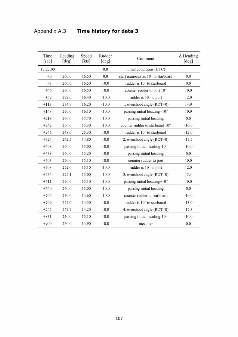
107
Appendix A.3 Time history for data 3
Time
[sec]
Heading
[deg]
Speed
[kts]
Rudder
[deg] Comment
Δ Heading
[deg]
17:22:00 0.0 initial conditions (UTC)
+0 260.0 16.50 0.0 start manoeuvre, 10° to starboard 0.0
+3 260.0 16.50 10.0 rudder is 10° to starboard 0.0
+46 270.0 16.50 10.0 counter rudder to port 10° 10.0
+52 272.0 16.40 -10.0 rudder is 10° to port 12.0
+113 274.9 16.20 -10.0 1. overshoot angle (ROT=0) 14.9
+148 270.0 16.10 -10.0 passing initial heading+10° 10.0
+218 260.0 15.70 -10.0 passing initial heading 0.0
+242 250.0 15.30 -10.0 counter rudder to starboard 10° -10.0
+246 248.0 25.30 10.0 rudder is 10° to starboard -12.0
+324 242.5 14.80 10.0 2. overshoot angle (ROT=0) -17.5
+408 250.0 15.00 10.0 passing initial heading-10° -10.0
+438 260.0 15.20 10.0 passing initial heading 0.0
+503 270.0 15.10 10.0 counter rudder to port 10.0
+508 272.0 15.10 -10.0 rudder is 10° to port 12.0
+534 275.1 15.00 -10.0 3. overshoot angle (ROT=0) 15.1
+611 270.0 15.10 -10.0 passing initial heading+10° 10.0
+640 260.0 15.00 -10.0 passing initial heading 0.0
+704 250.0 14.60 -10.0 counter rudder to starboard -10.0
+709 247.0 14.50 10.0 rudder is 10° to starboard -13.0
+745 242.7 14.20 10.0 4. overshoot angle (ROT=0) -17.3
+831 250.0 15.10 10.0 passing initial heading-10° -10.0
+900 260.0 14.90 10.0 meet her 0.0
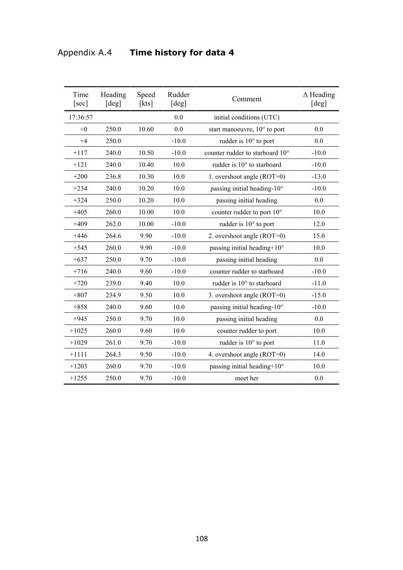
108
Appendix A.4 Time history for data 4
Time
[sec]
Heading
[deg]
Speed
[kts]
Rudder
[deg] Comment
Δ Heading
[deg]
17:36:57 0.0 initial conditions (UTC)
+0 250.0 10.60 0.0 start manoeuvre, 10° to port 0.0
+4 250.0 -10.0 rudder is 10° to port 0.0
+117 240.0 10.50 -10.0 counter rudder to starboard 10° -10.0
+121 240.0 10.40 10.0 rudder is 10° to starboard -10.0
+200 236.8 10.30 10.0 1. overshoot angle (ROT=0) -13.0
+234 240.0 10.20 10.0 passing initial heading-10° -10.0
+324 250.0 10.20 10.0 passing initial heading 0.0
+405 260.0 10.00 10.0 counter rudder to port 10° 10.0
+409 262.0 10.00 -10.0 rudder is 10° to port 12.0
+446 264.6 9.90 -10.0 2. overshoot angle (ROT=0) 15.0
+545 260.0 9.90 -10.0 passing initial heading+10° 10.0
+637 250.0 9.70 -10.0 passing initial heading 0.0
+716 240.0 9.60 -10.0 counter rudder to starboard -10.0
+720 239.0 9.40 10.0 rudder is 10° to starboard -11.0
+807 234.9 9.50 10.0 3. overshoot angle (ROT=0) -15.0
+858 240.0 9.60 10.0 passing initial heading-10° -10.0
+945 250.0 9.70 10.0 passing initial heading 0.0
+1025 260.0 9.60 10.0 counter rudder to port 10.0
+1029 261.0 9.70 -10.0 rudder is 10° to port 11.0
+1111 264.3 9.50 -10.0 4. overshoot angle (ROT=0) 14.0
+1203 260.0 9.70 -10.0 passing initial heading+10° 10.0
+1255 250.0 9.70 -10.0 meet her 0.0

109
Appendix A.5 Time history for data 5
Time
[sec]
Heading
[deg]
Speed
[kts]
Rudder
[deg] Comment
Δ Heading
[deg]
18:03:57 0.0 initial conditions (UTC)
+0 250.0 10.50 0.0 start manoeuvre, 20° to starboard 0.0
+5 250.0 10.50 20.0 rudder is 20° to starboard 0.0
+121 270.0 10.00 20.0 counter rudder to port 20 20.0
+129 273.0 9.90 -20.0 rudder is 20° to port 23.0
+152 275.5 9.50 -20.0 1. overshoot angle (ROT=0) 25.5
+231 260.0 9.50 -20.0 passing initial heading+20° 10.0
+331 250.0 9.00 -20.0 passing initial heading 0.0
+419 230.0 8.40 -20.0 counter rudder to starboard 20° -20.0
+430 227.0 8.40 20.0 rudder is 20° to starboard -23.0
+500 223.9 8.20 20.0 2. overshoot angle (ROT=0) -26.1
+542 230.0 8.30 20.0 passing initial heading-20° -20.0
+644 250.0 8.50 20.0 passing initial heading 0.0
+742 270.0 8.20 20.0 counter rudder to port 20.0
+751 273.0 8.20 -20.0 rudder is 20° to port 23.0
+812 274.7 8.10 -20.0 3. overshoot angle (ROT=0) 24.7
+851 270.0 8.30 -20.0 passing initial heading+20° 20.0
+957 250.0 8.40 -20.0 passing initial heading 0.0
+1051 230.0 8.00 -20.0 counter rudder to starboard -20.0
+1102 228.0 7.90 20.0 rudder is 20° to starboard -22.0
+1128 224.2 7.80 20.0 4. overshoot angle (ROT=0) -25.8
+1209 230.0 8.00 20.0 passing initial heading-20° -20.0
+1313 250.0 8.40 20.0 meet her 0.0

110
Lebenslauf
Persönliche Daten
Name: Daewon Kim
Geburtsdatum: 05.01.1983 in Daegu, Südkorea
Beruflicher Werdegang
03.2005 – 07.2008 Hanjin Shipping & Keoyang Shipping
- 2. Und 3. Nautische Offizier
08.2008 – 07.2011 Korea Maritime University, Institute of Marine Traffic Safety
- wissenschaftlicher Mitarbeiter
10.2013 – 10.2015 Hochschule Wismar, Institute ISSIMS
- wissenschaftlicher Mitarbeiter
Seit 12.2018 Universität Rostock, Institut für Automatisierungstechnik
- wissenschaftlicher Mitarbeiter
Studium
03.2001 – 02.2005 Bachelor of Engineering
Korea Maritime University, Department of Ship Operating Sys-
tem Engineering
03.2009 – 02.2011 Master of Engineering
Korea Maritime University, Department of Maritime Traffic In-
formation
Masterarbeit: „A Primary Study on the Development of Evalua-
tion Model for Marine Traffic Safety Assessment“
09.2011 – 08.2013 Master of Science
Hochschule Wismar, Master Studiengang für Operation and Man-
agement of Maritime Systems
Masterarbeit: „Optimization Methods for Modelling Simulator
Ship Models of a Ferry with Two Pairs of Azimuth Propellers”