Transportation Research Record 944 113

Estimating Trip Tables from Traffic Counts: Comparative

Evaluation of Available Techniques YEHUDA J. GUR

Methods for estimating trip tables from traffic counts are potentially useful because of their relative efficiency in data requirements. Two techniques for estimating existing trip tables in urban highway networks-the information theory (IT) technique and the LINKOD model-are analyzed in this paper. The separate description of the two techniques is followed by a formulation of an algorithm that is designed for application of the two techniques as well as other variations. By using the algorithm, extensive experimentation with the vari.ous techniques is made by using artificial data. Both the convergence speeds and the ability of the techniques to stay close to the target trip table are evaluated. The main contribution of the paper is its presentation of the two major techniques within an easily understood, unified format. It opens a way for extending the IT techniques for equilibrium assignment problems.

Much work has been done in recent years in develop­ing procedures for estimating trip tables from traf­fic counts. These methods are potentially useful because of their efficiency in terms of data re­quirements compared with the available alternatives. Chan et al. <.!I and Willis and Chan (~l recently compiled a comprehensive survey of the various esti­mating methods and the types of problems that they solve.

One type of problem is dealt with in this paper-­estimating an existing trip table for a typical urban highway network, based primarily on traffic counts on many links. Two different approaches to the problem have been reported. The first is the infor­mation theory (IT) approach, developed independently by Van Zuylen (3) and by Willumsen (4), and later described by Van Zuylen and Willumsen (5). The second is the network equilibrium approach -proposed by Nguyen (6-8) and extended by Gur et al. (.2,) into the LINKOD system.

The two methods have been developed independently from each other. Both have been developed primarily (but by no means exclusively) for estimating trip tables for •windows• in city centers. Recently, van Vliet and Willumi;;en (10) have reported the testing of the IT model on data from the center of Reading, England. Test application of LINKOD in downtown Washington, D.C., is reported by Gur et al. (9). Recently, a large-scale validation of LINKOD on data from downtown San Jose, California, has been re­ported by Han et al. (11) •

The purpose of this paper is to present the two methods by using a common basis, and to evaluate them comparatively. As a result of the evaluation, a third method, which uses some elements of each, is developed and tested.

DESCRIPTION OF PROBLEM

Consider a road network that consists of nodes con­nected by linksi some of the nodes are load nodes, where trips originate or terminate or both. It is assumed that trips between the load nodes are the only cause for traffic on the links. Given volume counts on some of the links, the problem is to find the true trip table T = (ti) that is served by the network. (Note that for simplicity of notation, ti denotes the ith cell in the table, giving the number of trips between two load nodes, e.g., k and (l).

There are three important attributes inherent to the problem. First, the solution requires assump­tions regarding the assignment rule, which d~scribes how travelers select their paths. Two different typ~ of assignment assumptions are possible. The

first is the proportional assignment where link volumes are directly proportional to the inter­changes served by them. This happens where path selection does not depend on link volume, as in an all-or-nothing assignment. Alternatively, with nonproportional assignment rules, path selection is a function of link volumes as in equilibrium assign­ment. Proportional assignment assumptions make the solution process simpler, but this assumption might be unrealistic in congested networks. The main body of this paper deals with all-or-nothing assignments.

A second important attribute of the problem is that in most cases there is no accurate solutionr i.e., there is no trip table that, when assigned (according to the assumed assignment rules), satis­fies exactly the given set of counts. This can happen both because of data imperfections (e.g., the counts are taken in different time periods) and modeling imperfections (e.g., the assumed assignment rule only approximates the actual route selection).

Third, in most cases the problem is underspeci­fiedi i.e., if there exists one table that satisfies a given set of flows, then there exist many other tables that, when assigned, produce those same flows. A complete solution method must address all these issues. It must be based on a realistic as­signment assumptioni it must be robust enough to withstand data inaccuracies and to estimate a table that approximates (rather than duplicates) the counts. It should also identify the best table among those that satisfy the counts.

Both the IT and the LINKOD models satisfy these requirementsi although LINKOD can operate for both proportional and equilibrium assignment assumptions, the current version of the IT model operates only for proportional assignment. The problem of multi­plicity of solutions is addressed in the two models in a similar way, i.e., the input to the model in-

. eludes a target trip table--a trip table that de­scribes the best estimate of the true table without traffic count information. The LINKOD model corrects this table as little as possible to approximate the observed flows. The IT model looks for the most likely, closest table to the target trip table that approximates the observed flows.

INFORMATION THEORY MODEL

Willumsen (4) developed a solution method based on entropy maximization considerations. The model (as well as a variation of it) is described by van Zuylen and Willumsen (~) • The problem is to find the maximum entropy trip table among those that satisfy the observed flows. Entropy of a table is defined as the number of micro states associated with it, weighted by probabilities that reflect the target trip table.

Van Zuylen and Willumsen (~) indicate that for the all-or-nothing assignment, the solution to the problem is of the form

where

t~ • ith element of the final trip table, fi a ith element of the target trip table,

(1)

114

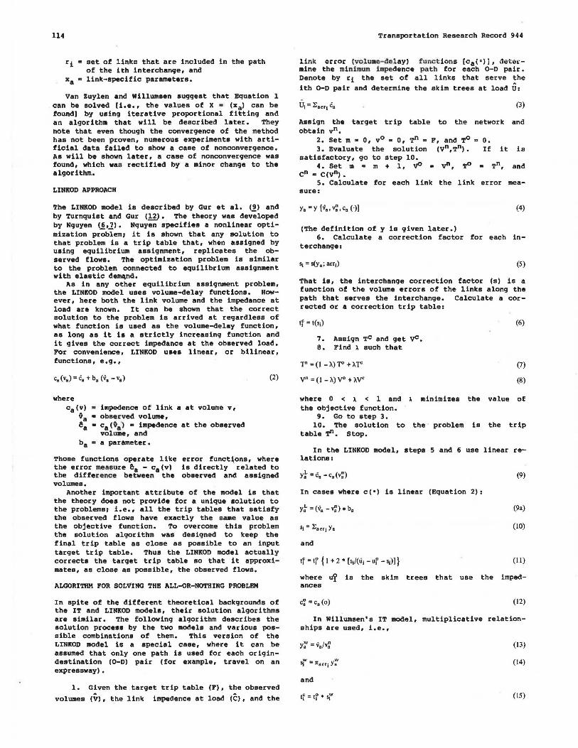
ri • set of links that are included in the path of the ith interchange, and

xa • link-specific parameters.

van Zuylen and Willumsen suggest that Equation 1 can be solved [i.e., the values of X • <xa> can be found) by using iterative proportional fitting and an algorithm that will be described later, They note that even though the convergence of the method has not been proven, numerous experiments with arti­ficial data failed to show a case of nonconvergence, As will be shown later, a case of nonconvergence was found, which was rectified by a minor change to the algorithm.

LINKOD APPROACH

The LINKOD model is described by Gur et al. <2> and by Turnquist and Gur (.!£). The theory was developed by Nguyen (_!,1>· Nquyen specifies a nonlinear opti­mization problemi it is shown that any solution to that problem is a trip table that, when assigned by using equilibrium assignment, replicates the ob­served flows. The optimization problem is similar to the problem connected to equilibrium assignment with elastic de~nd,

As in any other equilibrium assignment problem, the LINKOD model uses volume-delay functions. How­ever, here both the link volume and the impedance at load are known. It can be shown that the correct solution to the problem is arrived at regardless of what function is used as the volume-delay function, as long as it is a strictly increasing function and it gives the correct impedance at the observed load. For convenience, LINKOD uses linear, or bilinear, functions, e.g.,

where ca(v) • impedenee of link a at volume v,

•a • observed volume, ea • Ca (ta) • impedance at the observed

volume, and ba • a parameter.

(2)

Those functions operate like error funct~ons, where the error measure ea - ca(v) is directly related to the difference between the observed and assigned volumes,

Another important attribute of the model is that the theory does not provide for a unique solution to the problemsi i.e., all the trip tables that satisfy the observed flows have exactly the same value as the objective function. To overcome this problem the solution algorithm was designed to keep the final trip table as close as possible to an input target trip table, Thus the LINKOD model actually corrects the target trip table so that it approxi­mates, as close as possible, the observed flows.

ALGORITHM FOR SOLVING THE ALL-OR-NOTHING PROBLEM

In spite of the different theoretical backgrounds of the IT and LINKOD models, their solution algorithms are similar. The following algorithm describes the solution process by the two models and various pos­sible combinations of them. This version of the LINKOD model is a special case, where it can be assumed that only one path is used for each origin­destination (0-D) pair (for example, travel on an expressway),

1. Given the target trip table (F), the observed volumes (V), the link impedence at load (C), and the

Transportation Research Record 944

link error (volume- delay) functions [ca(•)), deter­mine the minimum impedence path for each 0-D pair. Denote by ri the set of all links that serve ~he

ith 0-D pair and determine the skim trees at load U:

(3)

Assign the target trip table to the network and obtain vn.

2. Set m • O, v0 • O, Tn = F, and To a o. 3. Evaluate the solution (Vn,Tn), If it is

satisfactory, go to step 10. 4. Set m = m + 1, Vo • vn, 'r° • Tn, and

en • C(Vn). s. Calculate for each link the link error mea­

sure:

(4)

(The definition of y is given later.) 6. Calculate a correction factor for each in­

terchange:

(5)

That is, the interchange correction factor (s) is a function of the volume errors of the links along the path that serves the interchange. Calculate a cor­rected or a correction trip table:

tf = t(s;) (6)

7. Assign Tc and get VC. e. Find A such that

1" = (1 - A) T" +AT"

vn = (1 - A) V0 + >.V0

(7)

(8)

where O < A < 1 and A minimizes the value of the objective function.

9. Go to step 3. 10. The solution to the · problem is the trip

table T". Stop.

In the LINKOD model, steps 5 and 6 use linear re­lations:

y} =Ca - Ca (v~) (9)

In eases where c(•) is linear (Equation 2):

S; = l:a•q Ya (10)

and

tf =tr { 1 +2 • [s1/(u1 -ur-s;)J} (11)

where uy is the skim trees that use the imped­ances

(12)

In Willumsen's IT model, multiplicative relation­ships are used, i,e.,

y'; =v.M (13)

st =naniY": (14)

and

tf=1r•sr (IS)

120

Table 2. Bias coefficienu for modal-choice disutility equatio111.

Income Coefficients

Group Automobile Automobile Drive Alone (I, I) (G, I)

Income Access Penalty Group• (I) Coefficient Coefficient !-Ratio Coefficient !-Ratio

Home-based work trips I 1.4165 1.4014 13.74 1.6733 21.14 2 1.0683 0.7979 8.24 1.2677 18.89 3 0.4943 -0.0750 -0.32 0.8939 10.01 4 -0.224; -0.6783 -6.59 0.6140 7.83

Home-based other trips 1 2.9661 0.0934 9.06 -1.5281 -24.40 2 2.3095 -1.1802 -21.00 -2.2168 -35.62 3 1.9305 -2.1397 -30.61 -2.7419 -44.41 4 1.4125 -2.9294 -38.33 -3 .1109 -50.70

Non-home-based trips 1 -1.3447 -11.73 -1.3496 -11.52 2 -1.9311 -17.53 -2.·1027 -17.19 3 -2.6904 -24.48 -2.5040 -21.67 4 -3.0689 -27.57 -2.7298 -23.35

Note: See Table 1 for equations used for bias coefficients. 8 Income groups are divided as follows : 1 = low, 2 =low-middle, 3 = high-middle , and

4 =high.

Table 3. Variables used in modal-choice calibration.

Acronym

Transit variables TRN RUN

AUTO ACC

WALK WAIT!

WAIT2

TXFER FARE AUTO CONN

TRN DACC 25

Highway variables H)VY RUN!

HWY RUNG

HWY CST!

HWYCSTG PRK CST! PRKCSTG HWYEXC

3

Units of Description of Variable Measure

In-vehicle time from the transit network, not Minutes including automobile access time

Automobile access time from the transit Minutes network

Walk access time from the transit network Minutes Transit boarding time for the first transit vehi· Minutes

cle from the transit network Time spent ·transferring from the transit Minutes

network Number of transfers from the transit network Number Transit fare Cents Dummy variable signifying if an automobile

was required to access the transit system (0 is no, 1 is yes)

Percentage of regional employment within 2 5 Percent min of total transit time from destination zone

Highway in-vehicle time from highway network for one person per car (drive alone) trips

Highway in-vehicle time for group automobile trips (same as HWY RUN I plus an additional time for each passenger)

Highway operating cost for one person per car trips

Highway operating cost for group trips Avg parking cost for one person per car trips Avg parking cost for group trips Time spent parking and unpacking an automo­

bile; the sum of highway terminal time at the origin zone and the destination zone (also called highway excess or terminal time)

Minutes

Minutes

Cents

Cents Cents Cents Minutes

C.l. = K/i~I [A(i) +CJ (1)

where

C.I. value of composite impedance, A(i) modal choice disutility function for mode i

(i - 1,2,3), c = constant chosen such that all A(i) 's are

positive, and K constant chosen such that all C.I. 's are

between 1 and 127, inclusive.

Transportation Research Record 944

This formula is simply the reciprocal of the sum of the modal impedances, scaled to represent suit­able values. The second formulation sums the expo­nential of the disutility function for all modes, takes the reciprocal of the sum, and takes the nat­ural loqarithm of this reciprocal. This is called the loq sum method, and is described as followss

(2)

Both of these functions meet the criteria previ­ously described, but little was known about the ability of either to perform as a measure of spatial separation. Therefore, both measures were tested by calibrating the home-based work trip-distribution model twice, each time by using a different mea­sure. The choice would then be made on the basis of whichever formulation provided the closer match to observed conditions, based on average trip length and other such measures.

CALIBRATION TECHNIQUE

The New Orleans distribution model uses the standard gravity model form (15). This model postulates that the number of trips for a given zone interchange is proportional to the number of trip productions at the origin zone and the number of trip attractions at the destination zone, and inversely proportional to the travel impedance between the two zones. The relationship with impedance is generally desci- ibed by a nonlinear function that relates impedance to a nondimensional F factor (also called friction factor).

The usual calibration process involves determin­ing the relationship between the impedance values and the F factors such that the distribution of es­timated trips by impedance matches that of the ob­served trips. Additional adjustment factors (K fac­tors) are used to help match observed and estimated trips by geographic stratification (such as dis­tricts). For this project, separate models were de­veloped for each trip purpose and for each of four income levels. Observed person trips came from the home interview survey.

Initially, it was assumed that the UTPS proqram AGM, operating in the so-called SAC mode, would be able to automatically calculate the proper F fac­tors. However, this function of program AGM was not operating correctly at that time and an ad-hoc method of calibrating the F factors was developed. This method used essentially the same technique as described in the AGM program documentation. F fac­tors are calculated by using a ga111111a function, i.e.,

F(I) = A • 18 * EXP (G * I)

where

F(I)

A,B, and G EXP=

F factor for impedance value I, calibrated coefficients, and exponential function.

(3)

This function was judged to be adequate because there is considerable documentation that it simu­lates the relationship between F factors and imped­ance adequately. Calibration of a distribution model consists mainly of fitting this curve. This was done as follows.

l. Apply program AGM in the apply-and-calibrate (AC) mode, which reports the observed and estimated trips stratified by each unit of impedance.

2. The observed and estimated trips and the F

Transportation Research Record 944

Tables l and 2. As the equations in Table l indi­cate, travel disutility is a linear function of the time and cost of the transit, drive alone, and group automobile modes, and other service characteristics such as number of transfers and transit accessibil­ity. Also, the income level of the traveler is a prime influence on perceived disutility. The dif­ferential effect of walk access to transit versus automobile access to transit on modal choice is de­fined through the use of an automobile access pen­alty dummy coefficient in the transit disutility equation. The variables are described in more de­tail in Table 3. For the work trip purpose, peak­hour impedance values were used; for home-based other and non-home-based purposes, off-peak values were used.

The mode and variable definitions for these equa­tions are similar to other modal-choice models re­cently developed for Minneai;lolis-St. Paul (~), Seat­tle (!.Q), Houston (11), St. Louis (il), and Buenos Aires (13). The group mode consists of persons in automobiles with two or more occupants. A separate logit submQdel is used to estimate the proportion of two-person, three-person, and four or more person trips in order to determine the average group occu­pancy for each interchange. The transit and highway variables are created from standard Urban Transpor­tation Planning System (UTPS) network analysis pro­grams (14) and special submodels are used to esti­mate a-;;;;essibility, terminal time, and parking cost. The calibration data consisted of a compre­hensive, home interview origin-destination survey conducted in the New Orleans region in 1960.

The coefficients and the final list of variables were developed by using ULOGIT on a sample of the survey file, followed by disaggregate validation and adjustment by using the full survey file. The coef­ficients are comparable to coefficients from other cities, exhibit internal consistency, and have ac­ceptable t-ratios (see Tables land 2). The 'follow­ing observations support the reasonableness of these equations1

Tabla 1. Modal-choice di1utility equations.

Mode Equation

119

1. The out-of-vehicle time coefficients exceed those for in-vehicle time;

2. The model is much more sensitive to automo­bile access time to transit than to time spent on the transit vehicle;

3. The ratio of the time coefficient to the cost coefficient, which is the implied value of travel time, is approximately one-third to one-half the av­erage 1960 regional income in cents per minute; and

4. The income bias coefficients indicate that as income level increases, there is a lower propensity to use transit, and within the automobile mode, a higher propensity to be a driver rather than a pas­senger.

COMPOSITE IMPEDANCE CALCULATION

The previous section describes how impedance is de­fined for each mode. The remaining challenge is to combine the three impedances into one value. For this task, the following conditions must be met.

l. The combined value must decrease as any of the modes becomes better, i.e., declines in time or cost.

2. The combined v~lue must increase if a mode is not available [i.e., an interchange with even unsat­isfactory transit service must have a better (lower) impedance than one with no service at all] •

3. The value must lie between l and 127, inclu­sive. The UTPS program AGM assumed that the input impedance values are stored as 1-byte matrix ele­ments. The highest value that can be represented in this format is 127.

4. The distribution of values within this range should l;>e reasonable; i.e., they should not be con­centrated at the top or bottom of the range.

It was ascertained that at least two mathematical formulations meet these criteria. One formulation is a variation of the harmonic mean function:

Home-based work trips Transit disutility 0.0332 • WALK+ 0.0769 • WAITl + 0.0319 • WAIT2 + 0.0078 • FARE+ 0.0145 • TRN RUN+ 0.1005 • AUTO ACC

Drive-alone disutility

Group automobile disutility

Home-based other trips Transit disutility

Drive·alone disutility

Group automobile disutility

Non-home-based trips Transit disutility

(4.07) (20.21) (8.85) (I0.45) (6.72) (2.59)

+ 0.0588 • TXFER +Auto Access Penalty (I) • AUTO CONN (3.59)

0.0693 •HWY EXC + 0.0145 •HWY RUN!+ 0.0078 •HWY CSTI + 0.02145 • PRK CSTI +Income Coefficient (I, I) (4.94) (6.72) (10.45) (ID.45)

0.0174 •HWY EXC + 0.0145 •HWY RUNG+ 0.0078 •HWY CSTG + 0.02145 • PRK CSTG +Income Coefficient (G, I) (1.74) (6.72) (10.45) (10.45)

0.0165 •(WALK+ WAITI + WAIT2) + O.ot 16 •FARE+ 0.0066 • (TRN RUN+ AUTO ACC)- 0.0183 • TRN DACC25 (7.45) (9.55) (-22.91)

+Auto Access Penalty (I) • AUTO CONN

0.3403 •HWY EXC + 0.0066 •HWY RUN!+ 0.0116 •HWY CSTI + 0.0319 • PRK CSTI +Income Coefficient (I, I) (25.98) (7.45) (9.55) (9.55)

0.2828 •HWY EXC + 0.0066 •HWY RUNG+ 0.0116 •HWY CSTG + 0.0319 • PRK CSTG +Income Coefficient (G, I) (28.50) (7.45) (9.55) (9.55)

0.0328 •(WALK+ WAITI + WAIT2) + 0.0047 • FARE+ 0.0131 • (TRN RUN+ AUTO ACC) + 0.0750 • TXFER (9.41) (2.75) (9.41)

+ 2.7472 •AUTO CONN (4.91)

Drive-alone disutility 0.2423 • HWY EXC + 0.0131 • HWY RUN I + 0.0047 • HWY CSTI + 0.0291 • PRK CSTI + Income Coefficient (I, I) (20.14) (9.41) (2.75) (2.75)

Group automobile disutility 0.3048 •HWY EXC + 0.0131 •HWY RUNG+ 0.0047 •HWY CSTG + 0.0291 • PRK CSTG +Income Coefficient (G, I) (25.58) (9.41) (2.75) (2.75)

Note: DIJutllltlH must be mulOplled by -1 b.etore taking the e)l:ponrintl•l in the lo1lt equation. Numbers in parentheses represent t-ratlos. T-ratlos were not calculated for the wo1k ind otho.r automobUo 1cc:m penalty (.Oc.tncients, or the nOn·homie-based co.:-tncient on TX FER. See Table 2 for explanation of bias coefficients used for the equations.