estimating the colored dissolved organic matter using 4d-var

Estimating the Colored Dissolved Organic Matter using 4D-Var

Suneet DwivediDepartment of Atmospheric and Ocean Sciences, University of Allahabad,

Allahabad, UP 211002, INDIA

&

Thomas HaineDepartment of Earth and Planetary Sciences, Johns Hopkins University, Baltimore,

MD 21218, USA

&

Carlos Del CastilloOcean Remote Sensing Group, Johns Hopkins University Applied Physics

Laboratory, Laurel, MD 20723, USA

Outline (Physical and Biogeochemical Data Assimilation):

Configuration and development of a limited area high-resolution numericalocean circulation model in support of SO GasEx oceanographic cruise.

configuration of associated 4D variational data assimilation software.

synthesize in-situ hydrographic data, CDOM data, and deliberately releasedpassive tracer data from the GasEx cruise with remotely-sensed observationsof CDOM, sea level and sea surface temperature.

execution and analysis of assimilation of physical and biogeochemical fields.

Coherent estimates of MLD

Modeling the photobleaching of Colored Dissolved Organic Matter (CDOM)and surface forcing of SF6.

• importance of understanding physical processes in Southern Ocean

• lack of observations

• huge size, high variability, sparseness of extant records

• approach: use a high-resolution ocean circulation model and optimallycombine it with the available observations using data assimilation

• data assimilation: state estimate

• estimates facilitate a wide range of studies in ocean circulation and itspractical applications

Southern Ocean Gas Exchange Experiment (GasEx): a research expedition

(Austral fall of 2008: Feb 29-Apr 12,2008; near South Georgia Island)

Objectives:

i) to measure and quantify air/sea gas transfer velocities at high winds, and tounderstand the influence of chemical and biological processes on the gasexchange

ii) reconcile the current discrepancy between model-based CO2 flux estimatesand observation-based estimates

• A particular aim is to understand how physical processes control theconcentration of Colored Dissolved Organic Matter (CDOM) in surfacewaters of the SO.

*CDOM: Degradation of biological material; degraded by photochemistry in euphotic zone

• estimation (abundance and distribution) of CDOM using DA

Task at hand:

• Ocean state estimation in the GasEx cruise region

• to bring a limited-area high-resolution ocean circulation model withrealistic physics into consistency with observations (in-situ and remotesensed) around the GasEx cruise region

• to describe the resulting physical and biogeochemical state of the ocean

The ECCO consortium : MITgcm + data + 4D-Var

Development of an ECCO configuration to perform data assimilation at O(1) km resolution in support of GasEx

High Resolution Forward Model:Hydrostatic MITgcm

4km (~1/25o)resolution, 36 levels (~106 cells) 6-hourly NCEP forcing;blended Sea-Winds

Initial hydrographic state from WOA05 climatologyPeriodic boundary conditions

KPP planetary boundary layer parametrizationHarmonic/Laplacian dissipation

MITgcm: ~325Km-550Km GasEx cruise: ~110Km-190Km

Southern Ocean (GasEx) Modeling and Ocean State Estimation

Adjoint Model/ Data Assimilation:

Adjoint code using TAFUnconstrained

minimization/Lagrange MultiplierObs: CTD T-S (GasEx Cruise),

SSH (AVISO), SST(AVHRR_AMSR_OI), CDOM,

SF6Optimization (successive

iteration) to minimize (least-square) objective/cost function (model-data

misfit)

SO GasEx Modeling and Data Assimilation

x(t+1) = Λ [x(t), Bq(t), Γu(t)]

1

0

2 ( 1) { ( 1) [ ( ), ( ), ( )]}J J Lt t t t tμ Γ−

=

′ = − + + −∑ft

T

t

x x Bq u

2 Jμ′∂

=∂y

1 1 1 1( )− − − −= +% T Tx E R E B E R y

1

1

10 0 0

11

0

[ ( ) ( ) ( )] ( ) [ ( ) ( ) ( )]

[ (0) ] [ (0) ]

( ) ( ) ( )

J tt t t t t t t

t t t

f

f

tT

t

b T b

t

t

y E x R y E x

x x P x x

u Q u

−

=

−

−−

=

= − −

+ − −

+

∑

∑

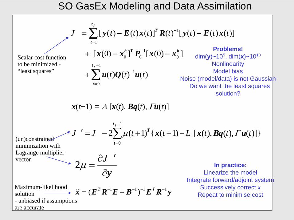
Scalar cost functionto be minimized -“least squares”

Maximum-likelihood solution- unbiased if assumptions are accurate

(un)constrained minimization with Lagrange multiplier vector

Problems!dim(y)~105, dim(x)~1010

NonlinearityModel bias

Noise (model/data) is not GaussianDo we want the least squares

solution?

In practice:Linearize the model

Integrate forward/adjoint systemSuccessively correct x

Repeat to minimise cost

Bathymetry:Smith and

Sandwell:1’

Advanced Very HighResolution Radiometer(AVHRR); AdvancedMicrowave ScanningRadiometer (AMSR);Optically Interpolated(OI) L4 gridded SST(oC) field

SST:

0.25o x 0.25o

Global

Daily

Interpolated to MITgcm grid

• time averaged SSH formal mapping error (cm)

• low along satellite track

Jason1 satellite track

ADT estimates sea surface heightrelative to the geoid (the theoreticalsurface of equal gravity around theEarth).

Multimission

0.25o x 0.25o

Global

Daily

Interpolated to MITgcm grid

NADT: proxy of merged gridded AVISO SSHanomaly (cm): normalized such that mean is zero

S. Dwivedi et al., J. Geophys. Res., 2011

•CTD Temperature and Salinity

•6 March 2008-5 April 2008

• 41 CTD profiles

•Bin averaged and interpolated to MITgcm grid

In-situ data


NormalizedAbsolute DynamicTopography (cm)


• GESE fits sealevel data manytime better thanother estimates

SST (oC)


• GESE fitsSST many timebetter thanother estimates

Model

CTD Obs


GESE solution is O(10-100)better than HYCOM+NCODAand ECCO-JPL

Ocean mixed layerdepth is calculatedbased on the shallowestextreme curvature ofnear surface layerdensity or temperatureprofiles: Lorbacher et al. 2006

** Particularlyimportant from thepoint of view of GasEx(relevant to upper oceanCDOM and evolution of SF6tracer patch)

Average MLD

Assimilation: 41 9 m

CTD obs.: 44 12 m

±

±


Estimates of MLD are important for a wide variety of oceanic investigations includingupper ocean productivity, air-sea exchange processes, and long-term climate change.

The assimilated field provides MLD estimates at places and times not sampled by theGasEx CTD.

Significant spatio-temporal variations are seen in the MLD during GasEx.

Is there any empirical link betweenspace/time MLD variations andsurface fields?

Space-time correlation of MLD with SSHA, SST and AT is –0.65, -0.51, and –0.52, respectively.

MLD* (m) = 823 – 11.6 SST (oC) + 0.30 NADT (m) – 2.62 AT (K).

Surface geostrophic velocity streamfunctions

OSCAR (Combination of Scatterometer and In-situ Data)

Important:

** No direct currentobservations were usedto constrain the model


Time varying estimates of:

net zonal volume flux (Sv) across section along western boundary

Net Ekman Flux: wind variability is not directly responsible for the net volume flux variability.


Colored dissolved organic matter (CDOM) is an optically activecomponent of the oceanic carbon pool.

It influences light penetration with consequences for primaryproductivity and the heat budget.

CDOM also interferes with remote sensing measurements ofchlorophyll.

With the advent of ocean color remote sensing, it becamepossible to study the global distribution of CDOM, and recentimprovements in algorithms have increased the accuracy of CDOMretrievals

However, the Southern Ocean (SO) is remote and cloudylimiting the availability of in-situ and ocean color data.

CDOM and SF6 Modeling:

Photobleaching of Colored Dissolved Organic Matter (CDOM)

aCDOM (λ, z) = aCDOM (λ) e –f (λ, z) Δt

where f (λ,z) is the vector of the photobleaching rate coefficients at wavelength λ, and depth zand is given by

f (λ, z) = σP (λ) E(λ) e –k (λ, z) z

where

σP (λ) is a matrix of photobleaching cross-section,

•E(λ) is the surface solar irradiance at wavelength λ, and

•k(λ, z) is the vertical attenuation constant which is approximated as (4/3) aCDOM (λ, z).

A package to simulate upper Ocean CDOM absorption coefficient was developed andcoupled with the MITgcm. In this context CDOM is, essentially treated as a passivetracer with time and space varying sources and sinks.

Biological sources of CDOM are likely negligible over the time scale of theresearch cruise and were ignored. Our working hypothesis is that CDOMdistribution in the mixed layer was controlled by mixing and photodegradation.

SF6 Modeling:

•The SF6 is considered as a passive tracer for modeling with the MITgcm.

•Following Wanninkhof [1992], a new code to simulate SF6 surface forcingis developed and included with the MITgcm.

•For this purpose, the air/sea tracer gas exchange flux was calculated asFexch = kp*(FXatm – Xsurf),

•where kp is the piston velocity (transfer coefficient), F is the gas solubility,and Xatm and Xsurf are gas concentrations in the atmospheric boundarylayer and at the ocean surface, respectively.

Time-mean satellitederived surface CDOMfields at each wavelengthare compared with thecorresponding GESE-CDOM surface CDOMfields.

MODIS – AQUA and SeaWiFS observations were available

The in-situ surface CDOM time series at 350nm, 380nm, and400nm, respectively at the cruise locations is compared with thecorresponding GESE-CDOM surface CDOM values in the SOGasEx domain.

• The in-situ CDOM (at allwavelengths) and SF6values are plotted againstthe corresponding GESE-CDOM fields.

• The slopes of the best-fitlines are 1.

• Most of the points on thescatter plots lie either on,or very close to, the best-fitline with only few pointsoutside the uncertaintyenvelope.

The mixed layer entrainment time scale:

Conclusions:• proof of concept: feasibility of performing such studies at very high resolutions:prototypical data assimilation system.

• possible to perform such kind of studies using moderate computationalresources; less expensive and loads of information (at desired very high spatial andtemporal resolution).

• basic physics is not too complicated and can be easily/quickly understood andimplemented.

• our high-resolution, regional data assimilation system that is customized toGasEx cruise successfully fits in-situ and satellite data

• provides best 4-dimensional (3-dimensional time-varying) estimate of physicalfields, CDOM and SF6 tracers in the locale of cruise.

• coherent estimates of mixed layer depth

• model CDOM estimates match very observations even without any biology in it.

In future: we shall explore the possibility of using SSH data from SARAL/AltiKa mission in our assimilation setup.

estimating the colored dissolved organic matter using 4d-var

Documents